PID Plus Adaptive Neural Network Control for Trajectory Tracking in Robotic Manipulators: Application to Automated Tape Laying (ATL)

Abstract

This article addresses the challenge of positioning accuracy in robotic manipulators applied to automated tape placement (ATL). A hybrid control strategy is proposed that integrates a Proportional-Integral-Derivative (PID) controller with a Backpropagation Neural Network (BP-NN). The proposed approach, called PID + NN, acts as a robust control scheme designed to compensate for parametric uncertainties and unmodeled perturbations arising from the integration of high-inertia tools in the end effector, dynamic mass variation due to tape consumption, and external reaction forces during the compaction process. Within this framework, the PID controller manages the nominal dynamics of the system, while the neural network operates as an adaptive compensator that adjusts the control signal in real time to minimize trajectory tracking errors. A rigorous stability analysis based on Lyapunov theory is presented, and the results are validated through numerical simulations on a six-degree-of-freedom manipulator. In addition, experimental tests are performed in a real operating environment to verify the practical performance of the strategy. The experimental results indicate that the proposed PID + NN controller significantly improves trajectory tracking accuracy, achieving a substantial reduction in tracking error and smoother control torque profiles compared to the conventional PID controller. These findings validate the effectiveness and robustness of the method for advanced manufacturing applications that demand high precision.

1. Introduction

Currently, the submarine and aerospace industries are imposing increasingly stringent technological requirements on the structural systems used in their applications. Consequently, components intended for these environments must meet rigorous specifications regarding their mechanical properties, particularly in terms of structural stiffness, mechanical strength, and operational reliability. Meeting these requirements has driven the development and implementation of advanced manufacturing processes, particularly automated tape laying (ATL) technology [1,2,3]. This process has established itself as one of the most widely used automated techniques in composite manufacturing, especially in the production of structures with simple geometries, characterized by relatively flat or gently curved surfaces [4]. The automation of the ATL process is achieved by integrating a specialized compaction head—known as an ATL head—into the end-effector of a robotic manipulator. This head is responsible for positioning, heating, and consolidating the resin-impregnated fiber tapes onto the mold surface, automatically replicating the principles of the traditional manual layup process [5].

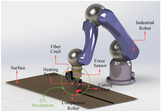
To ensure the structural quality of the final product, it is essential that the robotic manipulator position and orient the ATL head with a high degree of precision, strictly following the predefined path across the work surface. However, the ATL process introduces unique disturbances not present in conventional robotic tasks, such as the variable tension of the carbon fiber rolls and the dynamic interaction between the compaction roller and the mold surface. In this context, the performance of the manipulator control system plays a decisive role, as the accuracy of path tracking and the system’s ability to compensate for these specific external disturbances—including the variable mass of the tape reel during deposition—directly influence process efficiency and the quality of the resulting laminate [6,7,8]. Figure 1 illustrates the general architecture of the ATL system implemented on a regular surface, highlighting the main components of the ATL head developed in this work.

Figure 1. Six-axis industrial robot integrated with an automated tape-laying mechanism.

Traditionally, linear control strategies, such as the proportional-integral-derivative (PID) controller, have been widely adopted due to their simple structure and satisfactory performance, especially in systems operating near an equilibrium point. However, manipulators are highly nonlinear multivariable systems subject to unpredictable disturbances, which limits the performance of classical control schemes and drives the development of advanced control strategies [9,10]. Notable among these are PID-based approaches with hyperbolic functions [11], adaptive control [12,13], robust control [14,15], and sliding mode control [16], as well as hybrid methods that integrate state observers [17,18,19] or combine modern techniques with intelligent approaches such as neural networks [20,21,22,23]. In this context, neural network-based control systems have demonstrated great potential for adaptive learning and robust trajectory tracking in manipulators with multiple degrees of freedom [24,25,26,27,28], improving stability and accuracy in the presence of complex dynamics [29].

Despite these advances, the existing literature highlights significant challenges that limit the practical implementation of such strategies. First, the computational load of many intelligent controllers requires intensive offline training or high-end hardware for real-time execution. Second, the design complexity of robust techniques, such as sliding mode control, frequently generates vibrations—a detrimental effect that can damage the delicate ATL compaction mechanism. Finally, there is a serious lack of adaptability, as most current research on ATL control assumes constant process parameters and does not account for the dynamic disturbances inherent in carbon fiber deposition.

To address these limitations, this paper proposes a hybrid PID + NN control scheme applied to robotic manipulators in ATL processes. The proposed architecture combines the stability and simplicity of PID control with the adaptive learning capabilities of neural networks, with the aim of minimizing path-tracking errors and enabling online adaptation to external disturbances, dynamic variations, and unmodeled effects inherent in the manufacturing process. The main contribution of this work lies in providing a control law that facilitates real-time compensation for process-specific disturbances without the need for extensive prior training or high computational costs, thereby bridging the gap between advanced control theory and industrial feasibility.

Finally, this document is organized as follows: Section 2 presents the mathematical foundations of the robotic manipulator; Section 3 presents the development of the PID + NN control algorithm; Section 4 presents the evaluation of the controller in a simulation environment; Section 5 presents the experimental results obtained; and Section 6 presents the general conclusions of the study.

2. Mathematical Background of the Robotic Arm

2.1. Kinematic Model

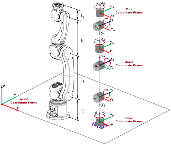
The robot considered in this study (see Figure 1) is a serial manipulator with 6 degrees of freedom (DoF), consisting of six actuators distributed across three sections (shoulder, elbow, and wrist, with two axes each), whose configuration mimics that of the human arm. Figure 2 shows the pose of the end-effector relative to the base system.

Figure 2. Representation of the initial position of the robot with the D-H convention.

The reference frames were assigned according to the D-H convention, allowing for a systematic description of the relationship between joint variables and the pose of the end-effector. Table 1 summarizes the D-H parameters corresponding to the analyzed manipulator robot.

Table 1. D-H parameters of the manipulator robot.

i	${\mathit{\theta }}_{\mathit{i}}$	${\mathit{d}}_{\mathit{i}}$	${\mathit{a}}_{\mathit{i}-1}$	${\mathit{\alpha }}_{\mathit{i}-1}$
1	${\theta }_i$	$l_0$	0	$-\pi /2$
2	${\theta }_2-\pi /2$	0	$l_1$	0
3	${\theta }_3+\pi /2$	0	0	$\pi /2$
4	${\theta }_4$	$l_2$	0	$-\pi /2$
5	${\theta }_5$	0	0	$\pi /2$
6	${\theta }_6$	$l_3$	0	0

The direct kinematics of the manipulator are obtained from the homogeneous transformation matrices, which allow the position $P_6^0$ and orientation $R_6^0$ of the end effector to be determined, as expressed in Equation (1):

$$H_6^0=H_1^0{H}_2^1{H}_3^2{H}_4^3{H}_5^4{H}_6^5=\left[\begin{array}{cccc}{n}_x& o_x& a_x& p_x\\ n_y& o_y& a_y& p_y\\ n_z& o_z& a_z& p_z\\ 0& 0& 0& 1\end{array}\right]=\left[\begin{array}{cc}{R}_6^0& P_6^0\\ 0_{1\times 3}& 1\end{array}\right]$$

(1)

where

$$\begin{array}{cc}\hfill n_x& =-s{\theta }_{6}c{\theta }_{4}s{\theta }_1-c{\theta }_{6}c{\theta }_{5}s{\theta }_{1}s{\theta }_4+c{\theta }_{23}c{\theta }_1\left[-s{\theta }_{6}s{\theta }_4-c{\theta }_6\left(s{\theta }_5-c{\theta }_{5}c{\theta }_4\right)\right]\hfill \\ \hfill n_y& =c{\theta }_1\left[s{\theta }_{6}c{\theta }_4+c{\theta }_{6}c{\theta }_{5}s{\theta }_4\right]+s{\theta }_1\left[s{\theta }_{23}\left(c{\theta }_{6}c{\theta }_{5}c{\theta }_4-s{\theta }_{6}s{\theta }_4\right)-c{\theta }_{23}c{\theta }_{6}s{\theta }_5\right]\hfill \\ \hfill n_z& =s{\theta }_{23}\left(s{\theta }_{4}s{\theta }_6+c{\theta }_{6}c{\theta }_{4}c{\theta }_5\right)-c{\theta }_{23}c{\theta }_{6}s{\theta }_5\hfill \\ \hfill o_x& =s{\theta }_1\left[s{\theta }_{6}c{\theta }_{5}s{\theta }_4-c{\theta }_{6}c{\theta }_4\right]+c{\theta }_1\left[-s{\theta }_{6}s{\theta }_{23}\left(\cos ({\theta }_5)c{\theta }_4+s{\theta }_5\right)+c{\theta }_{6}s{q}_{4}s{\theta }_{23}\right]\hfill \\ \hfill o_y& =c{\theta }_1\left[c{\theta }_{6}c{\theta }_4+s{\theta }_{6}c{\theta }_{5}s{\theta }_4\right]+s{\theta }_1\left[s{\theta }_{23}\left(c{\theta }_{6}s{\theta }_4+s{\theta }_{6}c{\theta }_{5}c{\theta }_4\right)-s{\theta }_{5}c{\theta }_{23}s{\theta }_6\right]\hfill \\ \hfill o_z& =s{\theta }_6\left(c{\theta }_{4}c{\theta }_{5}s{\theta }_{23}+s{\theta }_{5}c{\theta }_{23}\right)+c{\theta }_{6}s{\theta }_{23}s{\theta }_4\hfill \\ \hfill a_x& =c{\theta }_1(c{\theta }_{5}s{\theta }_{23}+s{\theta }_{5}c{\theta }_{4}c{\theta }_{23})-s{\theta }_{1}s{\theta }_{5}s{\theta }_4\hfill \\ \hfill a_y& =c{\theta }_{1}s{\theta }_{5}s{\theta }_4+s{\theta }_1(s{\theta }_{5}c{\theta }_{4}c{\theta }_{23}+c{\theta }_{5}s{\theta }_{23})\hfill \\ \hfill a_z& =c{\theta }_{5}c{\theta }_{23}-c{\theta }_{4}s{\theta }_{5}s{\theta }_{23}\hfill \\ \hfill p_x& =c{\theta }_1(s{\theta }_{23}[l_2-l_3(c{\theta }_5+c{\theta }_{4}s{\theta }_5)]-l_{1}s({\theta }_2))-l_{3}s{\theta }_{5}s{\theta }_{1}s{\theta }_4\hfill \\ \hfill p_y& =s{\theta }_1\left[l_{2}s{\theta }_{23}+l_3(\cos {\theta }_{5}s{\theta }_{23}+c{\theta }_{4}s{\theta }_{5}c{\theta }_{23})-l_{1}s{\theta }_2\right]+l_{3}s{\theta }_{5}c{\theta }_{1}s{\theta }_4\hfill \\ \hfill p_z& =l_0+l_{1}s{\theta }_2+c{\theta }_{23}\left(l_{3}c{\theta }_5+l_2\right)-s{\theta }_{23}{l}_{3}c{\theta }_{4}s{\theta }_5\hfill \end{array}$$

In these expressions, the abbreviated notation $s_i=\sin ({\theta }_i)$ and $c_i=\cos ({\theta }_i)$, as well as $s_{23}=\sin ({\theta }_2+{\theta }_3)$ and $c_{23}=\cos ({\theta }_2+{\theta }_3)$, in order to simplify the matrix representation of the kinematics. On the other hand, the inverse kinematics solution was divided into two stages: the first three joint variables ${\theta }_1,{\theta }_2,{\theta }_3$ were determined using the geometric method, while the remaining three joints ${\theta }_4,{\theta }_5,{\theta }_6$ were obtained by applying the principle of kinematic decoupling.

2.2. Dynamic Model and Properties

The dynamic model of a manipulator robot with n DoF, which considers the presence of perturbations and external forces, can be expressed by Equation (2):

$$M(q)\ddot{q}+C(q,\dot{q})\dot{q}+D(\dot{q})+g(q)+{\tau }_p=\tau$$

(2)

In this model, the vectors q, $\dot{q}$, $\ddot{q}\in {\mathbb{R}}^n$ represent, respectively, the position, velocity, and joint acceleration; $M(q)\in {\mathbb{R}}^{n\times n}$ is the inertia matrix, symmetric and positive definite; $C(q,\dot{q})\in {\mathbb{R}}^{n\times n}$ corresponds to the centripetal and Coriolis force matrix; $D\in {\mathbb{R}}^n$ is a positive semidefinite diagonal matrix that models viscous friction; $g(q)\in {\mathbb{R}}^n$ represents the gravitational force vector; $\tau \in {\mathbb{R}}^n$ denotes the control torque vector; ${\tau }_p\in {\mathbb{R}}^n$ groups together the perturbations applied to the system, such as the combined effect of external loads, unmodeled dynamics, and parametric variations in the environment, representing energy inputs not compensated for by the nominal model that challenge the controller’s robustness [30]. For the design of the controller and subsequent analysis of the system’s stability, the following standard properties and assumptions of the manipulator robot’s dynamics are considered. These are fundamental elements that are widely recognized and cited in the literature [30,31]:

Property 1.

The inertia matrix $M(q)\in {\mathbb{R}}^{n\times n}$ is symmetric and positive definite, so its inverse $M^{-1}(q)$ is also positive definite:

$$M(q)>0\mathrm{and}{M}^{-1}(q)>0⟹x^{T}M(q)x>0,\forall x\in {\mathbb{R}}^n$$

(3)

Property 2.

The centripetal–Coriolis matrix $C(q,\dot{q})$ and the time derivative of the inertia matrix $\dot{M}(q)$ satisfy the relation:

$${\dot{q}}^T\left[\frac{1}{2}\dot{M}(q)-C(q,\dot{q})\right]\dot{q}=0,\forall q,\dot{q}\in {\mathbb{R}}^n$$

(4)

which implies that the matrix $\dot{M}(q)-2C(q,\dot{q})$ is antisymmetric.

Property 3.

From Property 2, it follows that the time derivative of the inertia matrix and the centripetal–Coriolis matrix satisfy:

$$\dot{M}(q)=C(q,\dot{q})+C^T(q,\dot{q})$$

(5)

Property 4.

The left side of Equation (2) is linear with respect to the set of robot and load parameters, that is:

$$M(q)\ddot{q}+C(q,\dot{q})\dot{q}+D(\dot{q})+g(q)=Y\mathrm{\Theta }$$

(6)

where $Y\in {\mathbb{R}}^{n\times p}$ is the regressor matrix and $\mathrm{\Theta }\in {\mathbb{R}}^p$ is the vector that groups the unknown parameters of the manipulator and the load.

Assumption 1.

The unknown perturbations satisfy:

$$\parallel {\tau }_p\parallel \le b_d$$

(7)

where $b_d$ is a known positive constant [32].

3. Formulation and Design of the PID+Neural Network Controller

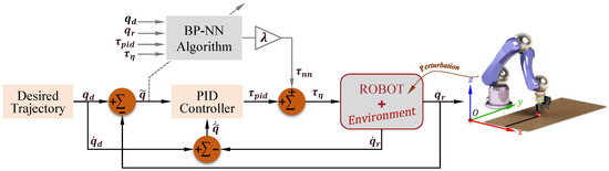
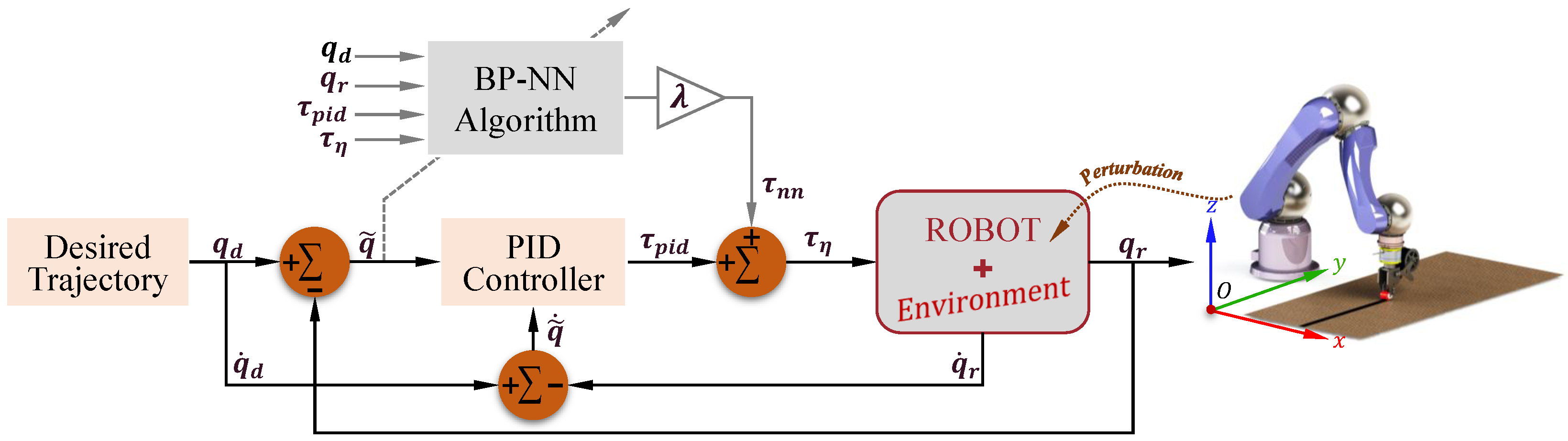
Modeling all the factors involved in the position control of robotic manipulators, particularly in tasks such as surface treatment, poses a significant challenge. These systems are influenced by multiple factors that affect their performance, including sensor noise and nonlinearities, differences between free and contact motion, communication delays, and material stiffness. Together, these effects create a dynamic, highly nonlinear, and uncertain environment, which makes it difficult to design control strategies that ensure stability and accuracy. Considering these limitations, a hybrid control scheme is proposed that combines the simplicity and stability of the classic PID controller with the learning and adaptation capabilities of an artificial neural network (NN). The general scheme, illustrated in Figure 3, integrates both approaches to improve the robustness of the system against external perturbations and dynamic variations inherent to the process.

Figure 3. Block diagram of the proposed PID + NN control system.

In the proposed control structure, the PID controller performs the main function of regulating the manipulator’s position and velocity via ${\tau }_{pid}$, while the NN Algorithm acts as an auxiliary controller that learns from the environment and generates a compensation signal ${\tau }_{nn}$ to correct the limitations of the classical scheme. This integration results in a control structure that is more robust against uncertainties and modeling errors, with its overall architecture formulated in Equation (8):

$${\tau }_{\eta }={\tau }_{pid}+{\tau }_{nn}$$

(8)

The control action ${\tau }_{pid}$ generated by the PID controller is defined by the following expression:

$${\tau }_{pid}=K_p\tilde{q}+K_i{\int }_0^t\tilde{q}dt+K_d\dot{\tilde{q}}$$

(9)

where $\tilde{q}$ is the joint position error, $\dot{\tilde{q}}$ is the velocity error and $K_p$, $K_i$, $K_d\in {\mathbb{R}}^{n\times n}$ are positive definite matrices corresponding to the proportional, integral, and derivative gains, respectively [31]. For its part, the signal ${\tau }_{nn}$ is modeled using a backpropagation neural network (BP-NN) with a single hidden layer, whose control action is described by:

$${\tau }_{nn}=\sigma \left[{\displaystyle \sum _{j=1}^1}{v}_{jk}\sigma \left[{\displaystyle \sum _{i=1}^n}{w}_{ij}{x}_i+w_i\right]+v_j\right]+ϵ$$

(10)

where $\sigma (·)$ is the activation function, $w_{ij}$ are the interconnection weights between the input layer and the hidden layer, $v_{jk}$ are the weights between the hidden layer and the output layer, and $ϵ$ represents a minimum approximation error vector of the NN bounded by $\parallel ϵ\parallel \le {ϵ}_N$ for some ${ϵ}_N>0$ [32].

Equation (10) can be rewritten in matrix form for a more compact representation:

$$f=V^T\sigma (W^{T}x)+ϵ$$

(11)

where $f={\tau }_{nn}$, $x={[x_1,x_2,\dots ,x_i]}^T$ is the input vector, $W^T={[w_{ij}]}^T$ and $V^T={[v_{jk}]}^T$ are the optimal weight matrices of the hidden and output layers, respectively.

Substituting the control actions into the dynamic equation of the manipulator, the resulting model is expressed as:

$$M(q)\ddot{q}+C(q,\dot{q})\dot{q}+D(\dot{q})+g(q)+{\tau }_p={\tau }_{\eta }$$

(12)

where ${\tau }_{\eta }$ finally defined as:

$${\tau }_{\eta }=K_p\tilde{q}+K_i\int \tilde{q}dt+K_d\dot{\tilde{q}}+V^T\sigma (W^{T}x)+ϵ$$

(13)

The composite control signal ${\tau }_{\eta }$ represents the sum of the actions of both controllers: the PID provides stability and immediate response to tracking errors, while the neural network introduces adaptability and dynamic compensation for nonlinearities and perturbations. This synergy improves the overall performance of the system and ensures more accurate trajectory tracking in complex industrial environments. The design and training of the proposed neural module are detailed below.

3.1. Adaptive Neural Network Topology

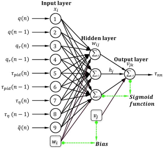
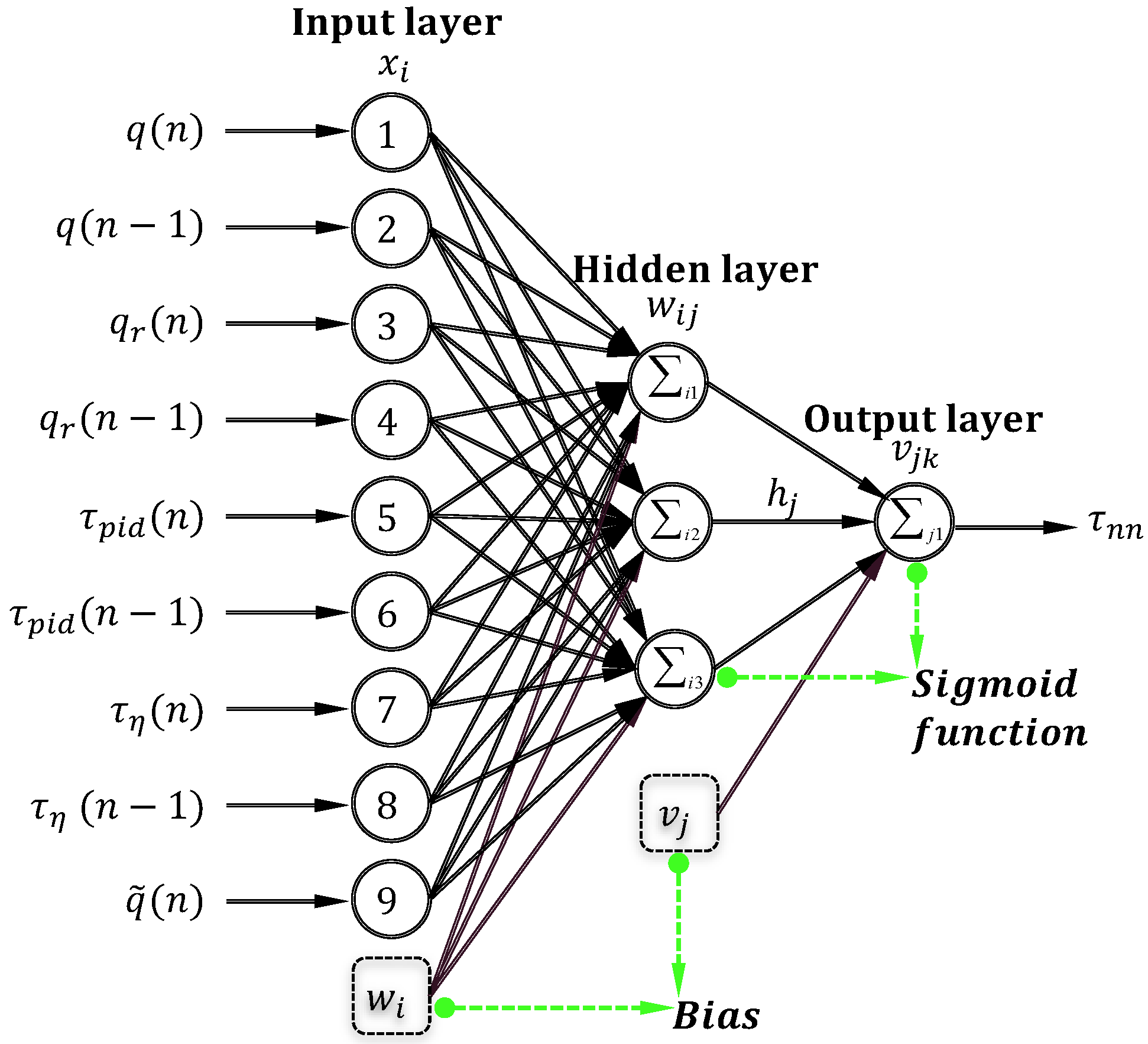
The topological structure of the NN is shown in Figure 4. The network consists of nine neurons in the input layer, three in the hidden layer, and one in the output layer. In the input layer, $q(n)$ and $q(n-1)$ represent the desired references, while $q_r(n)$ and $q_r(n-1)$ correspond to the actual reference outputs. Additionally, ${\tau }_{pid}(n)$ and ${\tau }_{pid}(n-1)$ denote the control signals generated by the PID controller, and ${\tau }_{\eta }(n)$ and ${\tau }_{\eta }(n-1)$ represent the combined control signals from the PID and the NN. Finally, $\tilde{q}(n)$ is defined as the joint position error.

Figure 4. Topological structure of the NN for trajectory tracking.

The sigmoid function was selected as the activation function for the hidden layer and output layer neurons due to its favorable mathematical properties: it is infinitely differentiable, allowing for efficient gradient calculation during backpropagation and facilitating model training convergence. The function is defined on $\mathbb{R}$ with a range of $(0,1)$, providing a continuous and smoothly stepped output.

The output of the neurons in the hidden layer is calculated using:

$$h_j={\displaystyle \frac{1}{1+e^{-s_j}}},s_j={\displaystyle \sum _{i=1}^3}{w}_{ij}{x}_i+w_i$$

(14)

Similarly, the network output, scaled by a gain factor $\lambda$, is defined as:

$${\tau }_{nn}={\displaystyle \frac{\lambda }{1+e^{-r_k}}},r_k={\displaystyle \sum _{j=1}^1}{v}_{jk}{h}_j+v_j$$

(15)

NN training is carried out using the backpropagation algorithm, with the cost function:

$$E(t)={\displaystyle \frac{1}{2}}{\displaystyle \sum _{k=1}^t}{(\tilde{q})}^2,\tilde{q}=q_r-q$$

(16)

where $\tilde{q}$ represents the joint position error.

The gradient of the cost function with respect to the network weights is calculated by applying the chain rule:

$$\nabla E(t)=\left[\begin{array}{c}{\displaystyle \frac{\partial E(t)}{\partial v_{jk}}}\\ {\displaystyle \frac{\partial E(t)}{\partial w_{ij}}}\end{array}\right]$$

(17)

For the weights of the output layer:

$$\begin{array}{cc}\hfill {\displaystyle \frac{\partial E(t)}{\partial v_{jk}}}& ={\displaystyle \frac{\partial E(t)}{\partial \tilde{q}}}{\displaystyle \frac{\partial \tilde{q}}{\partial e_{{\tau }_{\eta }}}}{\displaystyle \frac{\partial e_{{\tau }_{\eta }}}{\partial {\tau }_{nn}}}{\displaystyle \frac{\partial {\tau }_{nn}}{\partial r_k}}{\displaystyle \frac{\partial r_k}{\partial v_{jk}}}\hfill \\ \hfill & ={\delta }_k^1{h}_j{\displaystyle \frac{\partial \tilde{q}}{\partial e_{{\tau }_{\eta }}}},{\delta }_k^1=\tilde{q}\lambda {\tau }_{\eta }(1-{\tau }_{\eta })\hfill \end{array}$$

(18)

For the weights of the hidden layer:

$$\begin{array}{cc}\hfill {\displaystyle \frac{\partial E(t)}{\partial w_{jk}}}& ={\displaystyle \frac{\partial E(t)}{\partial \tilde{q}}}{\displaystyle \frac{\partial \tilde{q}}{\partial q_r}}{\displaystyle \frac{\partial q_r}{\partial {\tau }_{nn}}}{\displaystyle \frac{\partial {\tau }_{nn}}{\partial r_k}}{\displaystyle \frac{\partial r_k}{\partial h_j}}{\displaystyle \frac{\partial h_j}{\partial s_j}}{\displaystyle \frac{\partial s_j}{\partial w_{ij}}}\hfill \\ \hfill & =-{\delta }_j^2{x}_i{\displaystyle \frac{\partial \tilde{q}}{\partial e_{{\tau }_{\eta }}}},{\delta }_j^2={\delta }_k^1{v}_{jk}{h}_j(1-h_j)\hfill \end{array}$$

(19)

Finally, the network coefficients are adjusted using:

$$\begin{array}{cc}\hfill v_{jk}& =v_{jk}+\alpha {\displaystyle \frac{\partial \tilde{q}}{\partial e_{{\tau }_{\eta }}}}{\delta }_k^1{h}_j\hfill \end{array}$$

(20)

$$\begin{array}{cc}\hfill w_{ij}& =w_{ij}+\alpha {\displaystyle \frac{\partial \tilde{q}}{\partial e_{{\tau }_{\eta }}}}{\delta }_j^2{x}_i\hfill \end{array}$$

(21)

where $\alpha$ is the learning constant and ${\displaystyle \frac{\partial \tilde{q}}{\partial e_{{\tau }_{\eta }}}}$ can be interpreted as the equivalent gain of the unknown plant [33].

3.2. Adaptive Neural Network Training

The learning process was carried out autonomously and online, without requiring prior databases or prior knowledge of the system’s dynamics. However, to validate the robustness of this learning, a high-fidelity dynamic model developed in MATLAB/Simulink R2023b was used as an experimental environment. This model serves as the object of study, incorporating real physical parameters, nonlinear friction, and actuator dynamics, ensuring that the adaptation of the neural network weights occurs under realistic operating conditions.

Unlike conventional approaches based on offline data, the proposed method uses an online training strategy, in which the neural network’s learning process is directly integrated into the control loop. This enables real-time adaptation without the need for pre-collected datasets. At each sampling instant, the neural network receives the input vector defined as:

$$x(k)={[q(n),q(n-1),q_r(n),q_r(n-1),{\tau }_{pid}(n),{\tau }_{pid}(n-1),{\tau }_{\eta }(n),{\tau }_{\eta }(n-1),\tilde{q}(n)]}^T$$

(22)

where $q(n)$ is the reference, $q_r$ is the measured output, and $\tilde{q}$ is the joint position error.

The training was performed using the backpropagation algorithm based on the gradient of the cost function $E(t)$ (Equation (16)), updating the weights online and in real time according to the learning rules defined in Equations (20) and (21). The initial weights of the hidden layer neurons ($w_{ij}$) and the output layer ($v_{jk}$) were randomly assigned values from the set $-1, 0, 1$. The learning rate $\alpha$ were both set to $0.01$ for all degrees of freedom, selected empirically to ensure stable convergence during online training and to maintain an adaptive response to variations in the system dynamics. This formulation allows the neural network to continuously adapt to changes in the environment and the nonlinear dynamics of the system, improving the real-time tracking of manipulator trajectories.

3.3. Stability and Convergence Analysis

Due to Property 4 of linear parameterization, Equation (12) can be expressed in terms of a nominal reference ${\dot{q}}_r$ and its derivative ${\ddot{q}}_r$, yielding:

$$M(q){\ddot{q}}_r+C(q,\dot{q}){\dot{q}}_r+D(\dot{q})+g(q)+{\tau }_p=\widehat{Y}\mathrm{\Theta }$$

(23)

where $\widehat{Y}=\widehat{Y}(q,\dot{q},{\dot{q}}_r,{\ddot{q}}_r)\in {\mathbb{R}}^{n\times p}$.

By adding and subtracting Equation (23) from the Equation (12), we obtain the open-loop error equation:

$$M(q)(\ddot{q}-{\ddot{q}}_r)+C(q,\dot{q})(\dot{q}-{\dot{q}}_r)={\tau }_{\eta }-\widehat{Y}\mathrm{\Theta }$$

(24)

The approximate value of $\widehat{Y}\mathrm{\Theta }$ is given by the following expression:

$$\widehat{Y}\mathrm{\Theta }\equiv {\widehat{V}}^T\sigma ({\widehat{W}}^{T}x)$$

(25)

where $\widehat{V}$ and $\widehat{W}$ are the current values of the NN weights obtained using the weight adjustment algorithm specified in the previous section.

Using the definition of the filtered tracking error, the following relationship holds:

$$\begin{array}{cc}\hfill s& =\dot{\tilde{q}}+\mathrm{\Lambda }\tilde{q}+\mathrm{\Gamma }\int \tilde{q}dt\hfill \end{array}$$

(26)

where $s\in {\mathbb{R}}^n$ denotes the filtered error, $\tilde{q}=q-q_r$ represents the joint position error, and $\mathrm{\Lambda },\mathrm{\Gamma }>0$. Under this definition, the control action ${\tau }_{\eta }$ can be rewritten in terms of the filtered error:

$$\begin{array}{cc}\hfill {\tau }_{\eta }& =-K_D\mathrm{\Lambda }\tilde{q}-K_D\mathrm{\Gamma }\int \tilde{q}dt-K_D\dot{\tilde{q}}+V^T\sigma (W^{T}x)+ϵ\hfill \\ \hfill & =-K_{D}s+V^T\sigma (W^{T}x)+ϵ\hfill \end{array}$$

(27)

where $K_D>0$ parameterizes the proportional and integral gains as $K_p=K_D\mathrm{\Lambda }$ and $K_i=K_D\mathrm{\Gamma }$.

Substituting the control action ${\tau }_{\eta }$ and the approximate value of $\widehat{Y}\mathrm{\Theta }$ into Equation (24) yields the closed-loop error dynamics:

$$M\dot{s}+Cs=[-K_{D}s+V^T\sigma (W^{T}x)+ϵ]-[{\widehat{V}}^T\sigma ({\widehat{W}}^{T}x)]$$

(28)

Grouping terms:

$$M\dot{s}=-K_{D}s+\tilde{f}-Cs$$

(29)

In this context, $\tilde{f}$ represents the neural network’s approximation error and can be expressed as:

$$\begin{array}{cc}\hfill \tilde{f}& =f-\widehat{f}\hfill \\ \hfill & =V^T\sigma (W^{T}x)+ϵ-{\widehat{V}}^T\sigma ({\widehat{W}}^{T}x)\hfill \end{array}$$

(30)

where f represents the unknown ideal continuous function and $\widehat{f}$ is its respective estimation. In order to cancel terms in the Lyapunov derivative $\dot{L}$, we need to express this difference in terms of the weight errors $\tilde{V}=V-\widehat{V}$ and $\tilde{W}=W-\widehat{W}$. Adding and subtracting the term $V^T\sigma ({\widehat{W}}^{T}x)$, Equation (30) expands as follows:

$$\begin{array}{cc}\hfill \tilde{f}& =V^T\sigma (W^{T}x)-V^T\sigma ({\widehat{W}}^{T}x)+V^T\sigma ({\widehat{W}}^{T}x)-{\widehat{V}}^T\sigma ({\widehat{W}}^{T}x)+ϵ\hfill \\ \hfill & =V^T[\sigma (W^{T}x)-\sigma ({\widehat{W}}^{T}x)]+(V^T-{\widehat{V}}^T)\sigma ({\widehat{W}}^{T}x)+ϵ\hfill \\ \hfill & =V^T\sigma ({\tilde{W}}^{T}x)+(V^T-{\widehat{V}}^T)\sigma ({\widehat{W}}^{T}x)+ϵ\hfill \\ \hfill & =V^T\sigma ({\tilde{W}}^{T}x)+{\tilde{V}}^T\sigma ({\widehat{W}}^{T}x)+ϵ\hfill \end{array}$$

(31)

To approximate the term $\sigma ({\tilde{W}}^{T}x)=\sigma (W^{T}x)-\sigma ({\widehat{W}}^{T}x)$, we use a Taylor series expansion of $\sigma (W^{T}x)$ around $\sigma ({\widehat{W}}^{T}x)$:

$$\begin{array}{cc}\hfill \sigma (W^{T}x)& =\sigma ({\widehat{W}}^{T}x)+\dot{\sigma }({\widehat{W}}^{T}x){\tilde{W}}^{T}x+O{({\tilde{W}}^{T}x)}^2\hfill \end{array}$$

(32)

where $O{({\tilde{W}}^{T}x)}^2\le c_i$ are the higher-order terms of the Taylor series and $c_i$ is a computable positive constant. Therefore, Equation (31) can be rewritten as:

$$\begin{array}{cc}\hfill \tilde{f}& ={\tilde{V}}^T\sigma ({\widehat{W}}^{T}x)+{\widehat{V}}^T[\dot{\sigma }({\widehat{W}}^{T}x){\tilde{W}}^{T}x+O{({\tilde{W}}^{T}x)}^2]+ϵ\hfill \end{array}$$

(33)

Let $\dot{\widehat{\sigma }}=\dot{\sigma }({\widehat{W}}^{T}x)$, then we obtain:

$$\begin{array}{cc}\hfill \tilde{f}& ={\tilde{V}}^T\widehat{\sigma }+{\widehat{V}}^T{\widehat{\sigma }}^{\prime }{\tilde{W}}^{T}x+\zeta \hfill \end{array}$$

(34)

where $\zeta$ is the bounded perturbation term that includes higher-order Taylor errors and the network approximation error ($ϵ$).

Theorem 1.

Consider the dynamic model of the robot given by Equation (2), under the action of the control law ${\tau }_{\eta }$ defined in Equation (13). Then, the closed-loop system described by Equation (29) guaranties that the position and velocity tracking errors $\tilde{q},\dot{\tilde{q}}$ are asymptotically stable, provided that the control gains are positive and the weights W and V are updated according to:

$$\dot{\widehat{W}}=Gx{({\widehat{\sigma }}^{\prime T}\widehat{W}s)}^T$$

(35)

$$\dot{\widehat{V}}=F\widehat{\sigma }{s}^T$$

(36)

where F and G are symmetric positive-definite gain matrices, s is the filtered tracking error, $\widehat{\sigma }$ denotes the sigmoid activation function evaluated at the current weights, ${\widehat{\sigma }}^{\prime }$ is the derivative of the activation function, and x represents the input vector to the NN [32].

Proof. 

Let the following be the Lyapunov candidate function:

$$L={\displaystyle \frac{1}{2}}{s}^{T}Ms+{\displaystyle \frac{1}{2}}\mathrm{tr}({\tilde{W}}^T{G}^{-1}\tilde{W})+{\displaystyle \frac{1}{2}}\mathrm{tr}({\tilde{V}}^T{F}^{-1}\tilde{V})$$

(37)

Deriving L with respect to time:

$$\begin{array}{cc}\hfill \dot{L}& =s^{T}M\dot{s}+{\displaystyle \frac{1}{2}}{s}^T\dot{M}s+\mathrm{tr}({\tilde{W}}^T{G}^{-1}\dot{\tilde{W}})+\mathrm{tr}({\tilde{V}}^T{F}^{-1}\dot{\tilde{V}})\hfill \end{array}$$

(38)

Substituting $\dot{M}s$ as given by Equation (29):

$$\begin{array}{cc}\hfill \dot{L}& =s^T[-K_{D}s+\tilde{f}-Cs]+{\displaystyle \frac{1}{2}}{s}^T\dot{M}s+\mathrm{tr}({\tilde{W}}^T{G}^{-1}\dot{\tilde{W}})+\mathrm{tr}({\tilde{V}}^T{F}^{-1}\dot{\tilde{V}})\hfill \\ \hfill & =-s^T{K}_{D}s+s^T\tilde{f}+{\displaystyle \frac{1}{2}}{s}^T(\dot{M}s-2C)s+\mathrm{tr}({\tilde{W}}^T{F}^{-1}\dot{\tilde{W}})+\mathrm{tr}({\tilde{V}}^T{G}^{-1}\dot{\tilde{V}})\hfill \end{array}$$

(39)

Using Property 2 of the manipulator’s dynamics:

$$\dot{L}=-s^T{K}_{D}s+s^T\tilde{f}+\mathrm{tr}({\tilde{W}}^T{G}^{-1}\dot{\tilde{W}})+\mathrm{tr}({\tilde{V}}^T{F}^{-1}\dot{\tilde{V}})$$

(40)

Substituting $\tilde{f}$ from Equation (34):

$$\dot{L}=-s^T{K}_{D}s+s^T({\tilde{V}}^T\widehat{\sigma }+{\widehat{V}}^T{\widehat{\sigma }}^{\prime }{\tilde{W}}^{T}x+\zeta )+\mathrm{tr}({\tilde{W}}^T{G}^{-1}\dot{\tilde{W}})+\mathrm{tr}({\tilde{V}}^T{F}^{-1}\dot{\tilde{V}})$$

(41)

By rearranging the terms using the trace properties, specifically $s^T{\tilde{V}}^T\widehat{\sigma }=\mathrm{tr}({\tilde{V}}^T\widehat{\sigma }{s}^T)$, we obtain:

$$\dot{L}=-s^T{K}_{D}s+\mathrm{tr}\left[{\tilde{V}}^T(F^{-1}\dot{\tilde{V}}+\widehat{\sigma }{s}^T)\right]+\mathrm{tr}\left[{\tilde{W}}^T(G^{-1}\dot{\tilde{W}}+x{s}^T{\widehat{V}}^T{\widehat{\sigma }}^{\prime })\right]+s^T\zeta$$

(42)

On the other hand, assuming that the ideal weights of the neural network ($W,V$) are constant ($\dot{W}=0,\dot{V}=0$), the relationship between the error in the weights ($\tilde{W},\tilde{V}$) and their estimates ($\widehat{W},\widehat{V}$) is expressed in terms of their time derivatives as:

$$\dot{\tilde{W}}=-\dot{\widehat{W}},\dot{\tilde{V}}=-\dot{\widehat{V}}$$

(43)

This result indicates that any update to the network tuning law ($\dot{\widehat{W}},\dot{\widehat{V}}$) directly affects the dynamics of the weight error. By substituting these dynamics and the selected adaptation rules into the derivative of the Lyapunov function, the trace terms cancel out, ensuring that:

$$\dot{L}\le -s^T{K}_{D}s+s^T\zeta$$

(44)

Since the Lyapunov function is positive definite ($L>0$) and its derivative is negative semidefinite ($\dot{L}\le 0$), the system is guaranteed to be stable in the Lyapunov sense. This condition ensures that the tracking error vector s and the neural network weight errors ($\tilde{V},\tilde{W}$) remain bounded at all times. Additionally, the integrability of $\dot{L}$ shown in Equation (45) allows us to conclude, via Barbalat’s Lemma, the asymptotic convergence of the tracking error.

$${\int }_0^{\infty }-\dot{L}dt<\infty$$

(45)

□

4. Numerical Simulation

Based on the dynamic model defined in Equation (13), together with the dynamic parameters of the Schunk Powerball LWA 4P manipulator reported in [34] and the specifications of the ERB-115 and ERB-145 actuators [35], a simulator was developed in MATLAB/Simulink to systematically analyze the dynamic behavior and performance of the system under different operating conditions, serving as a basis for the comparative evaluation of control strategies. The specifications for the ERB-115 and ERB-145 actuators are shown in Table 2.

Table 2. Technical specifications of the ERB-115 and ERB-145 modules.

Specification	Unit	ERB-115	ERB-145
Max Speed	$°/\mathrm{s}$	72	72
Nominal Torque	Nm	7	35
Max Torque	Nm	19	64
Max rotation angle	$°$	340	340
Weight	kg	1.8	3.9

4.1. Simulator Configuration and Controller Parameters

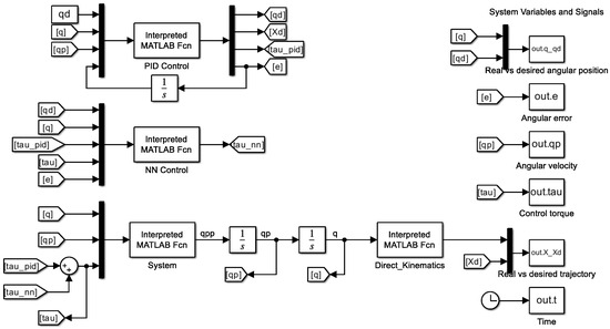
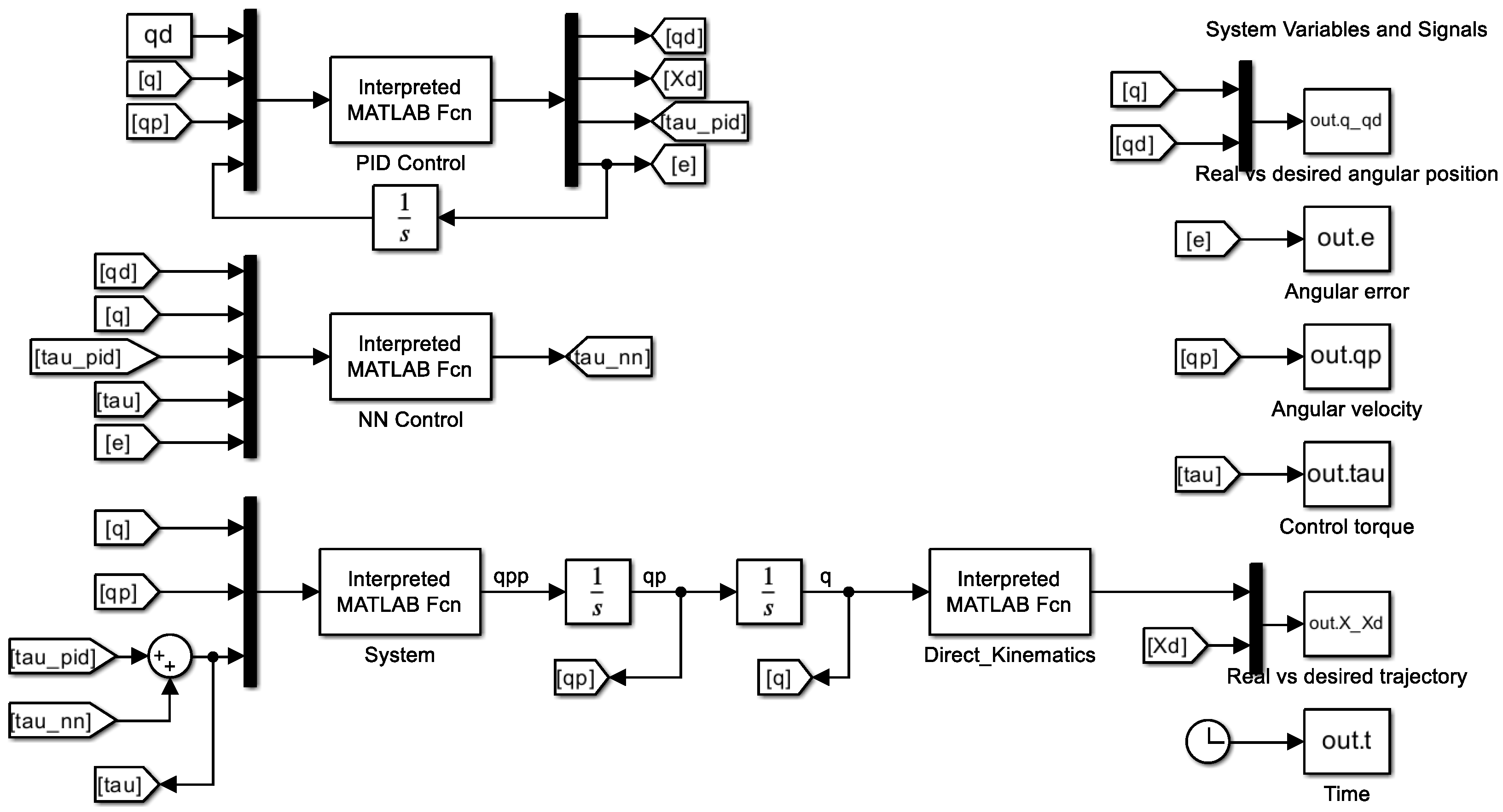
Figure 5 shows the overall architecture of the mathematical model and incorporates two control schemes: a classical PID controller and a neural network-based control system.

Figure 5. Block diagram of the Powerball LWA 4P robot simulator.

The block called System represents the complete dynamics of the manipulator, solving the equations of motion using two cascade integrators that generate the joint position and velocity variables. From these variables, the Direct Kinematics block calculates the Cartesian position of the end effector. On the right side of the diagram are the output blocks, which allow the main variables of the system to be recorded and analyzed, such as the desired and actual joint position, angular error, joint velocity, control torque, and Cartesian trajectory. These data were used to evaluate the dynamic performance and tracking accuracy of the implemented control strategies. The PID control gains were determined heuristically; the values used for the simulation were: $K_p=diag([60,60,55,45,35,35])$, $K_i=diag([0.5,0.5,0.5,0.5,0.5])$ and $K_d=diag([25,25,25,25,25,25])$. The ODE45 method was used for numerical integration with a time step of $t=0.001\mathrm{s}$.

4.2. Reference Trajectory Generation CAD-Based

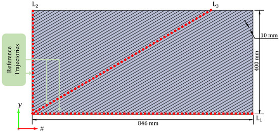
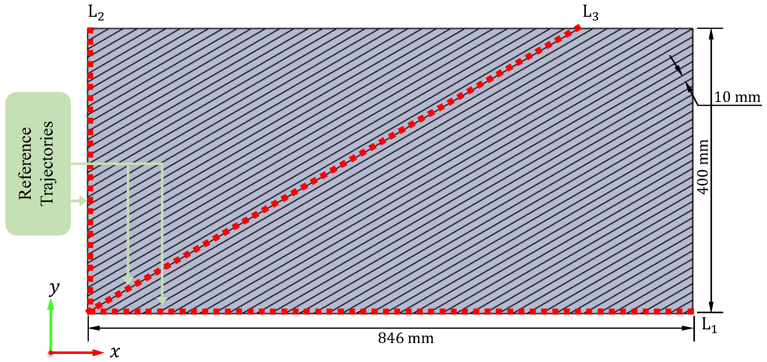
To evaluate the robustness and performance of the proposed PID + NN control scheme, experiments were conducted in three scenarios using reference trajectories that differed in length and angular orientation. The reference trajectories were generated from a CAD model representing a flat surface $846\mathrm{mm}$ long and $400\mathrm{mm}$ wide, as shown in Figure 6.

Figure 6. Test surface for trajectory tracking.

This surface was discretized into parallel strips spaced $10\mathrm{mm}$ apart, incorporating patterns with orientations of $0^{\circ }$, ${30}^{\circ }$, and ${90}^{\circ }$. The selection of this spacing and the corresponding orientations was based on the target application, which focuses on the manipulation of carbon fiber composite material strips $10\mathrm{mm}$ wide, whose deposition trajectories typically exhibit angular variations between layers.

4.3. Simulation Scenarios and Results

The proposed approach was subjected to the following simulation scenarios:

(a)

Scenario I. In this scenario, trajectory $L_1$ is evaluated, characterized by a length of 0.846 m and an orientation of $0^{\circ }$ relative to the x-axis.

(b)

Scenario II. In this scenario, trajectory $L_2$ is evaluated, characterized by a length of 0.400 m and an orientation of ${90}^{\circ }$ relative to the x-axis.

(c)

Scenario III. In this scenario, trajectory $L_3$ is evaluated, characterized by a length of 0.800 m and an orientation of ${30}^{\circ }$ relative to the x-axis.

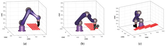
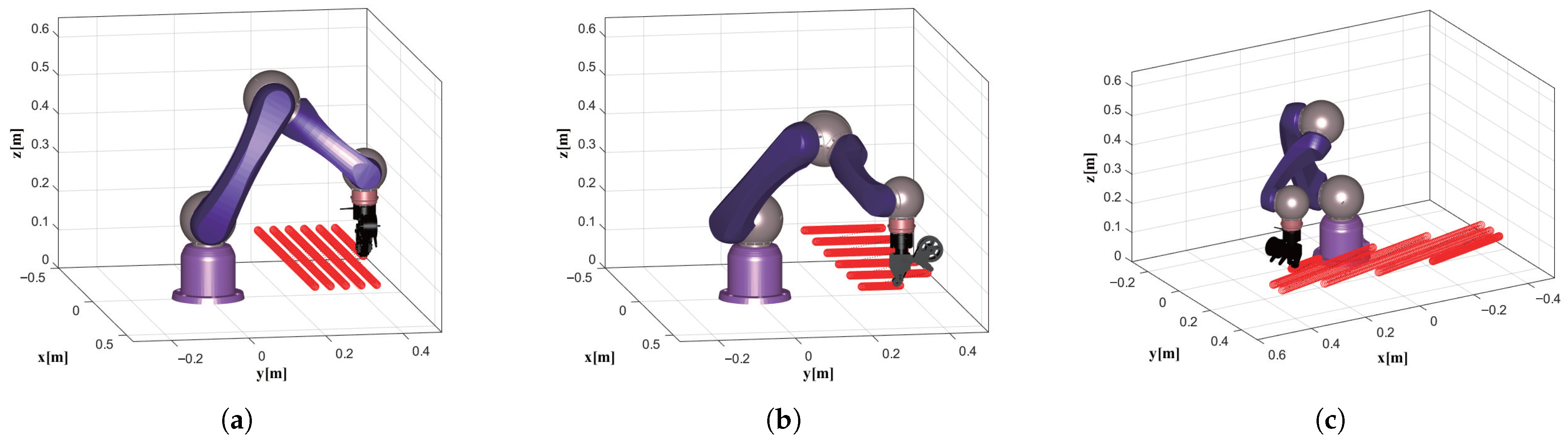
Figure 7 shows the execution of the three scenarios by the robotic manipulator in a 3D virtual environment. The initial position and orientation of the end effector were defined as $x=-0.4\mathrm{m}$, $y=0.2\mathrm{m}$, $z=0.18\mathrm{m}$, $roll=0^{\circ }$, $pitch={\displaystyle \frac{\pi }{2}}$, and $yaw=0^{\circ }$. The manipulator robot begins with an initial error of $0.08\mathrm{m}$ position. A constant forward velocity of $v=0.01\mathrm{m}/\mathrm{s}$ was maintained throughout all tests. Figure 8, Figure 9, Figure 10, Figure 11, Figure 12, Figure 13, Figure 14, Figure 15, Figure 16, Figure 17, Figure 18, Figure 19, Figure 20 and Figure 21 allow for a more detailed analysis of the robot’s behavior during the tracking of test trajectories for each scenario considered.

Figure 7. Tracking test trajectories in a 3D virtual environment: (a) Scenario I. (b) Scenario II. (c) Scenario II.

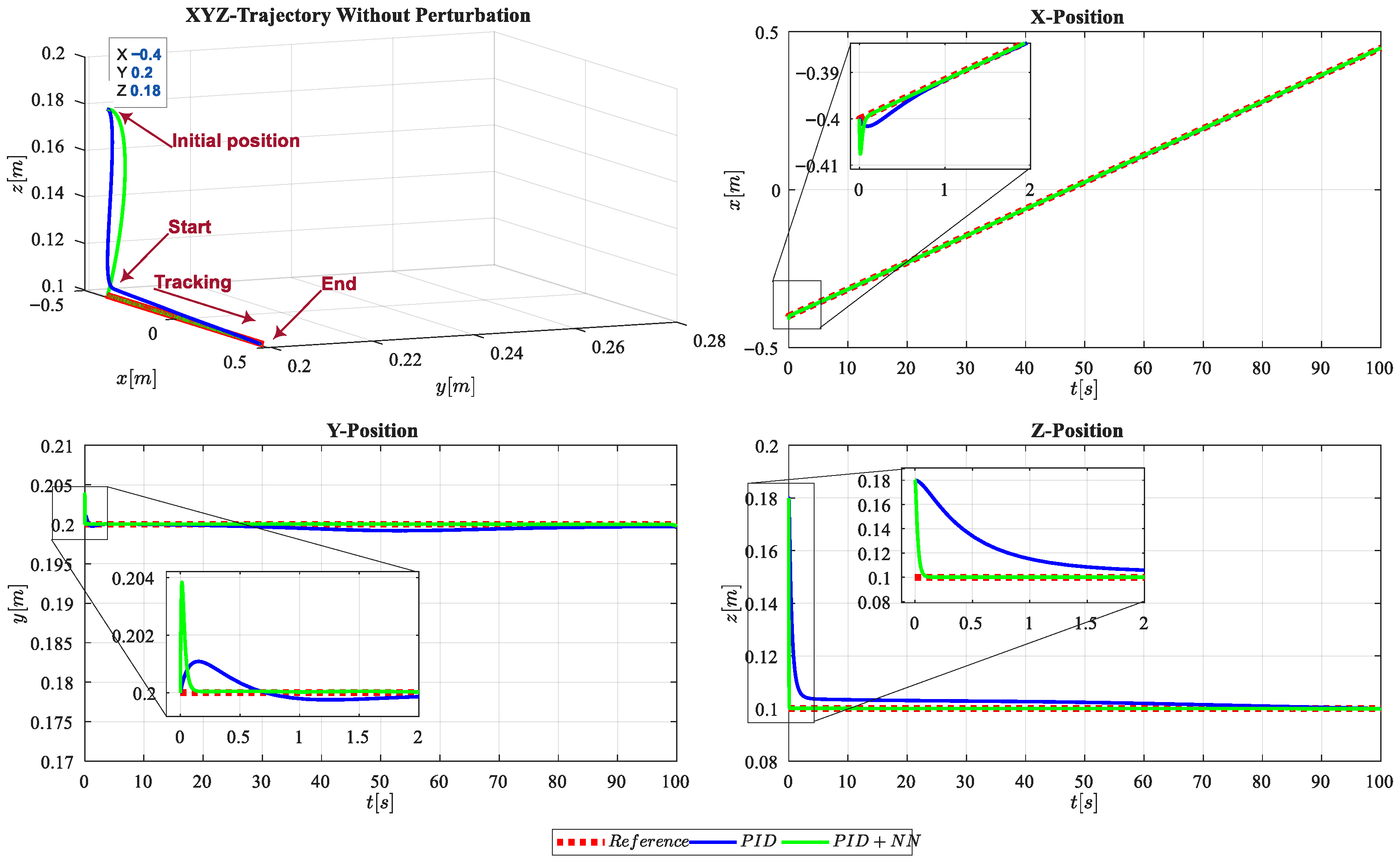
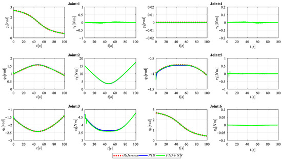
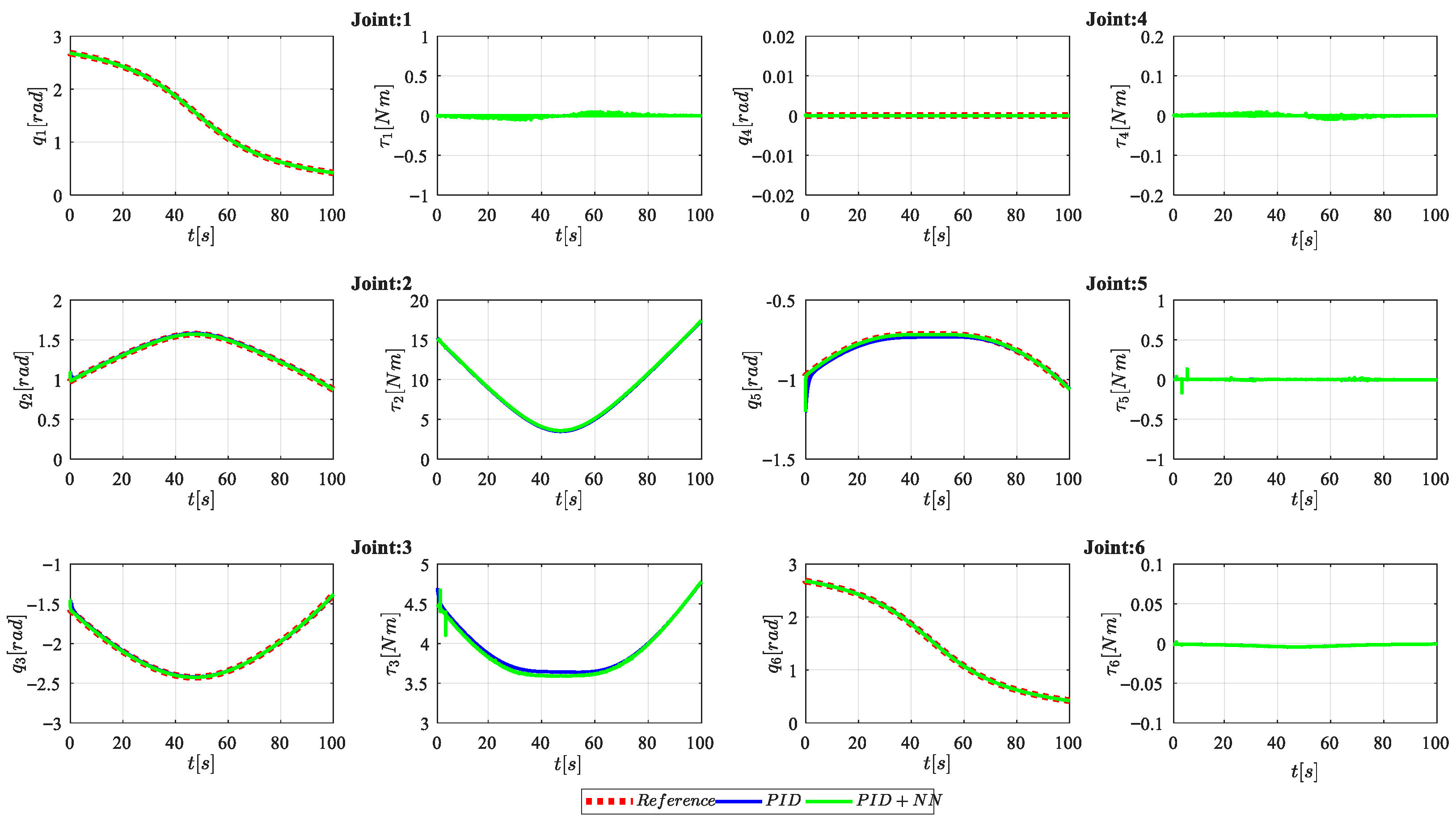
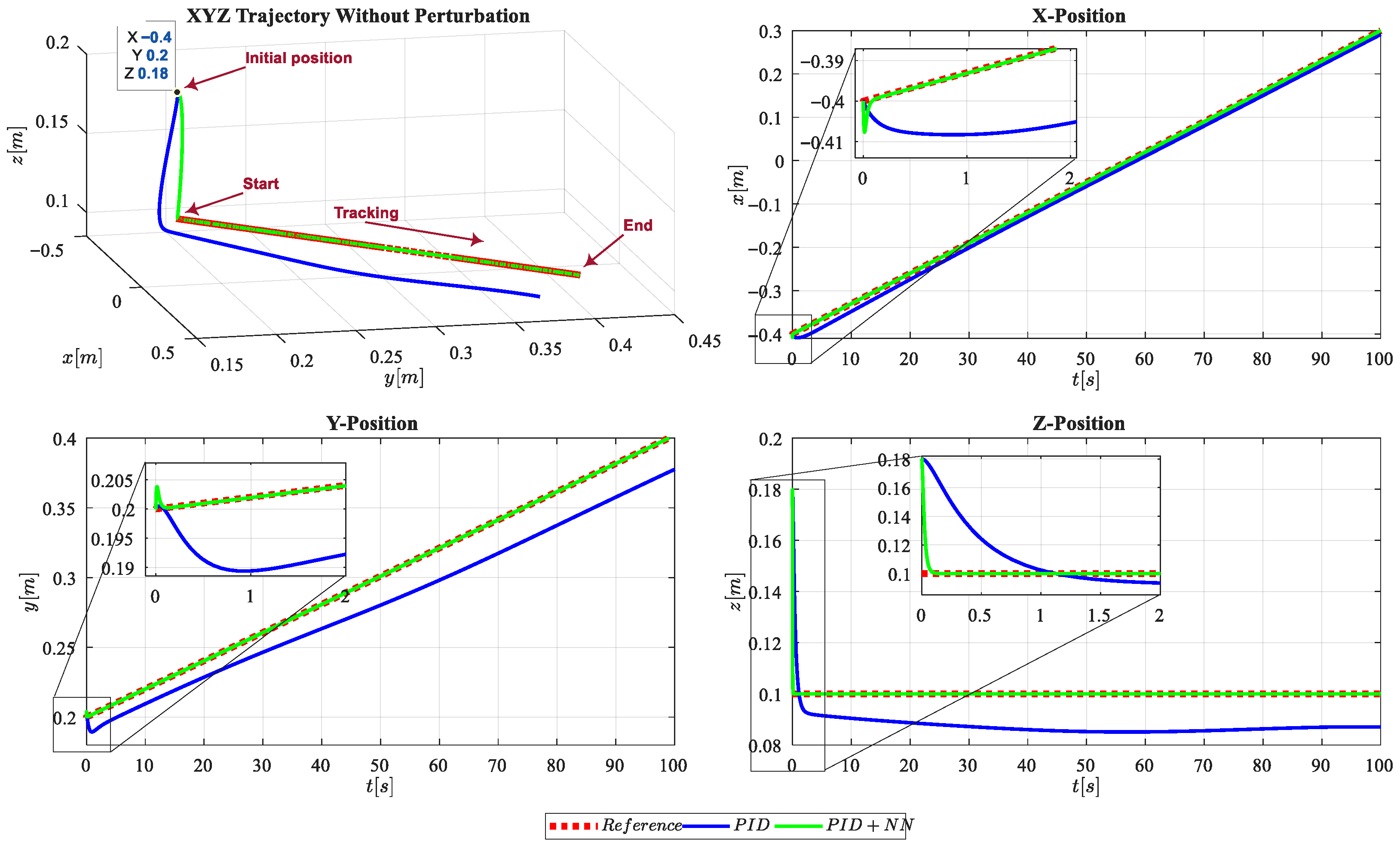
Figure 8. Tracking the $L_1$ trajectory under nominal conditions: ideal reference (red dotted line), classical PID (blue line), and PID + NN (green line).

Figure 9. Joint angular positions $q_i$ and control torques ${\tau }_i$ along the $L_1$ trajectory under nominal conditions.

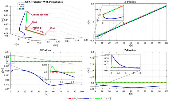
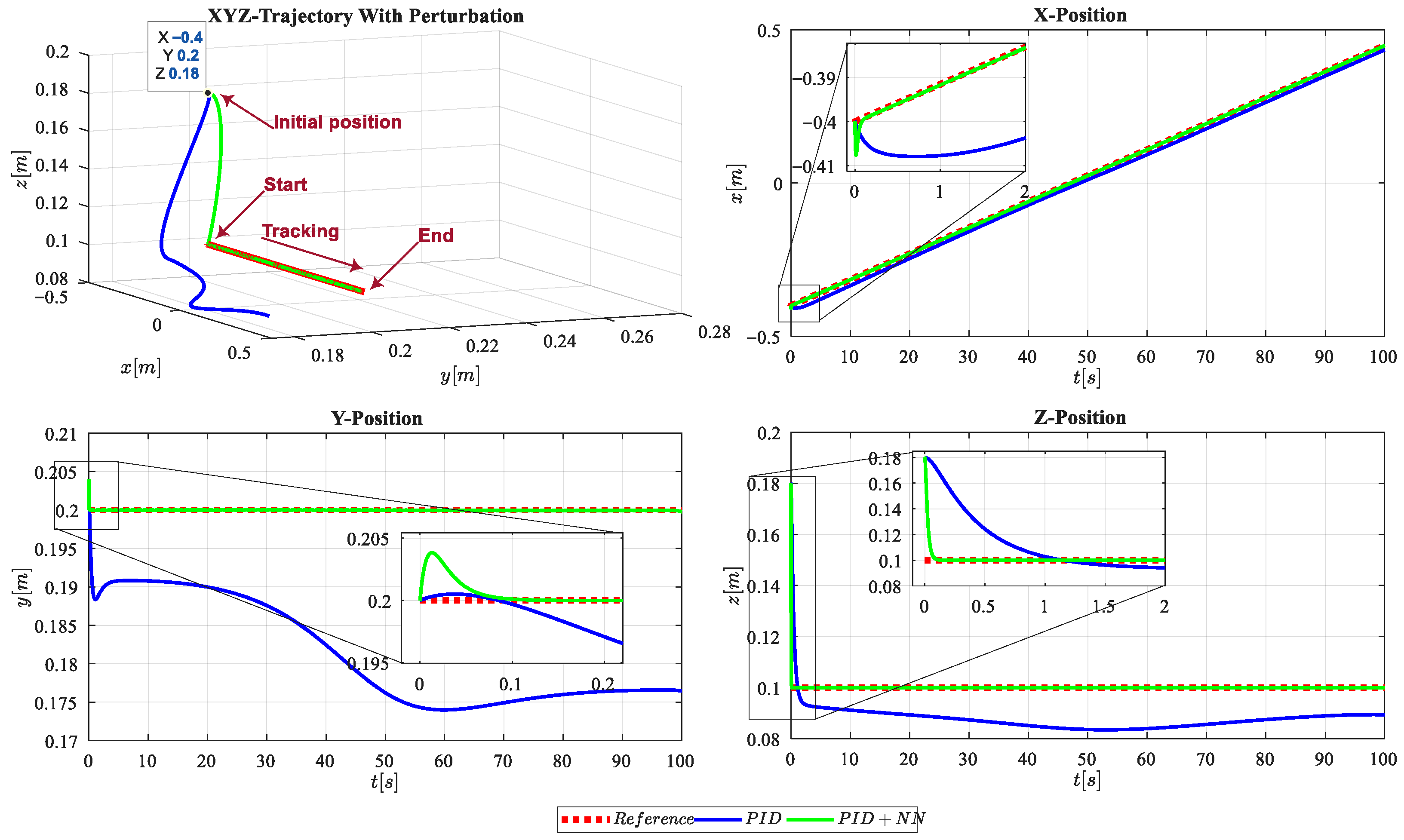
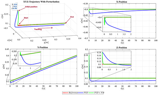
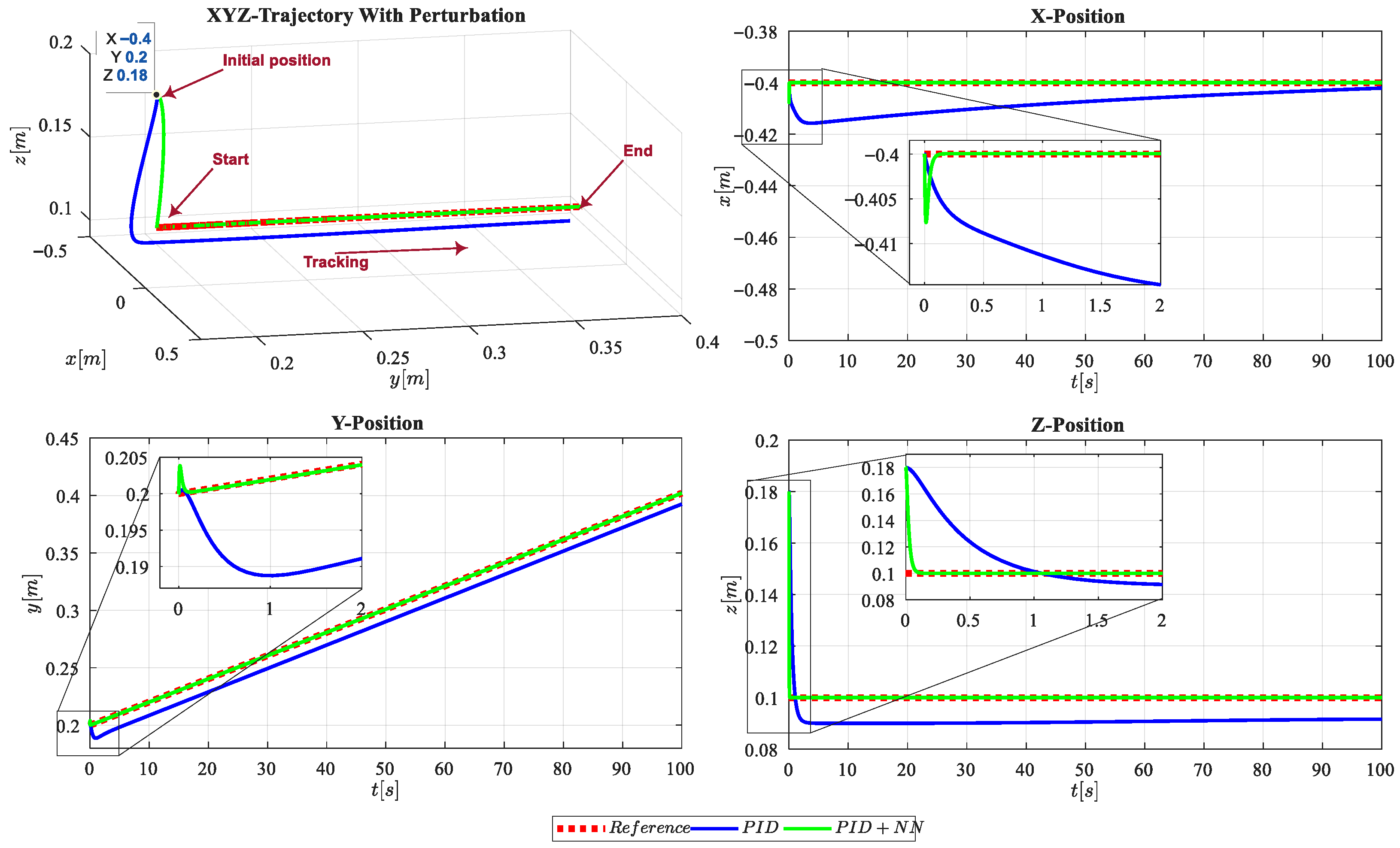
Figure 10. Tracking the $L_1$ trajectory under perturbation: ideal reference (red dotted line), conventional PID (blue line), and PID + NN (green line).

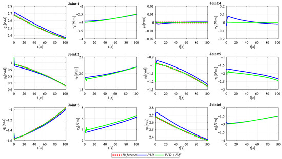
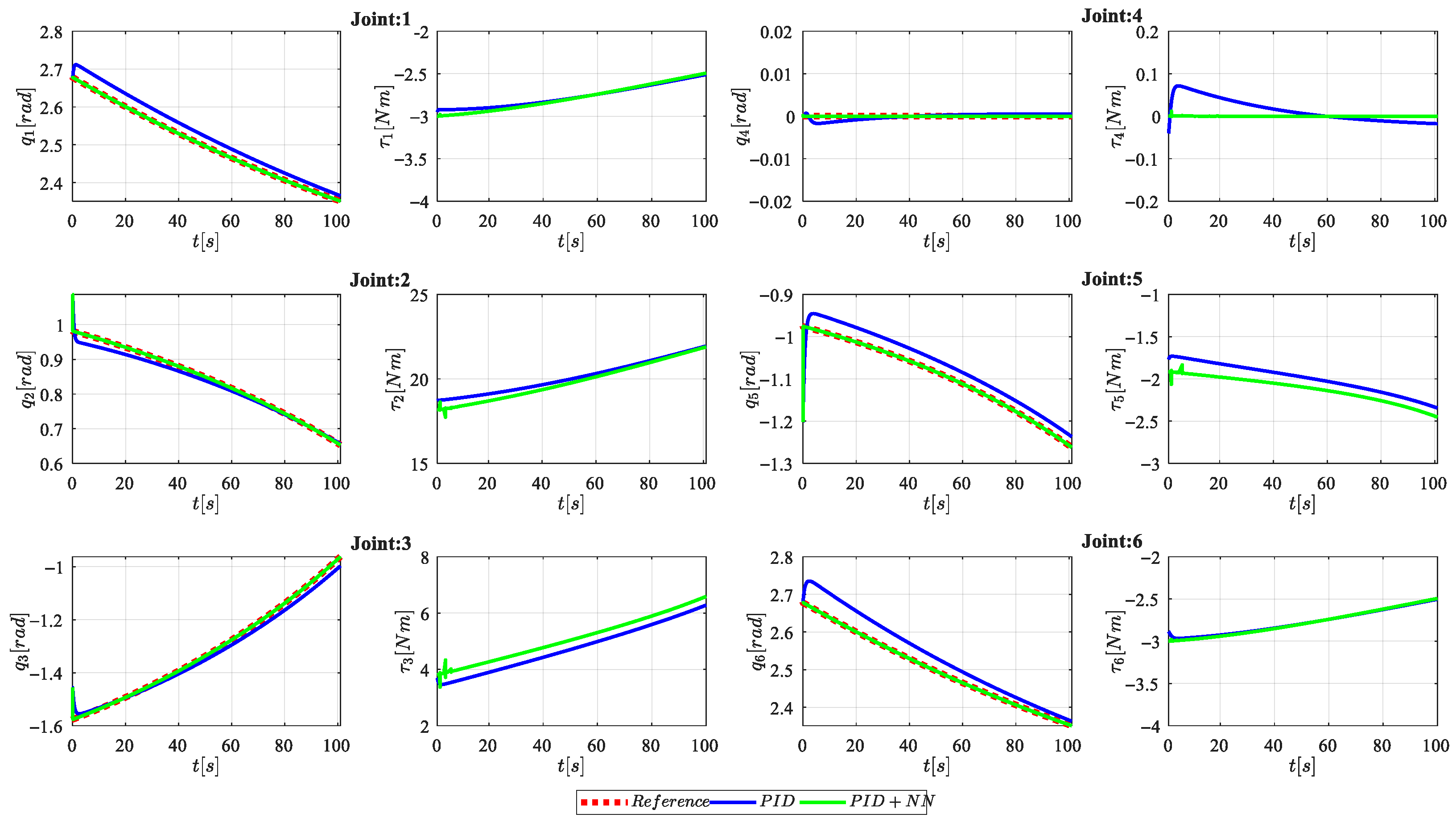
Figure 11. Joint angular positions $q_i$ and control torques ${\tau }_i$ along the $L_1$ trajectory under perturbation.

Figure 12. End-effector Cartesian tracking error in Scenario I.

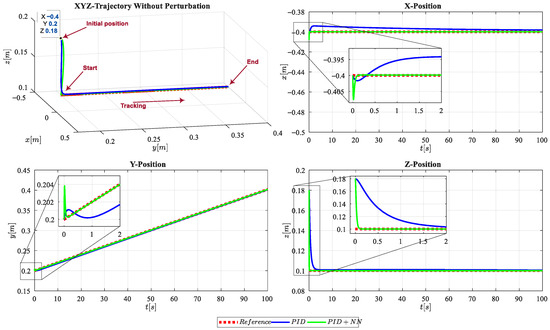
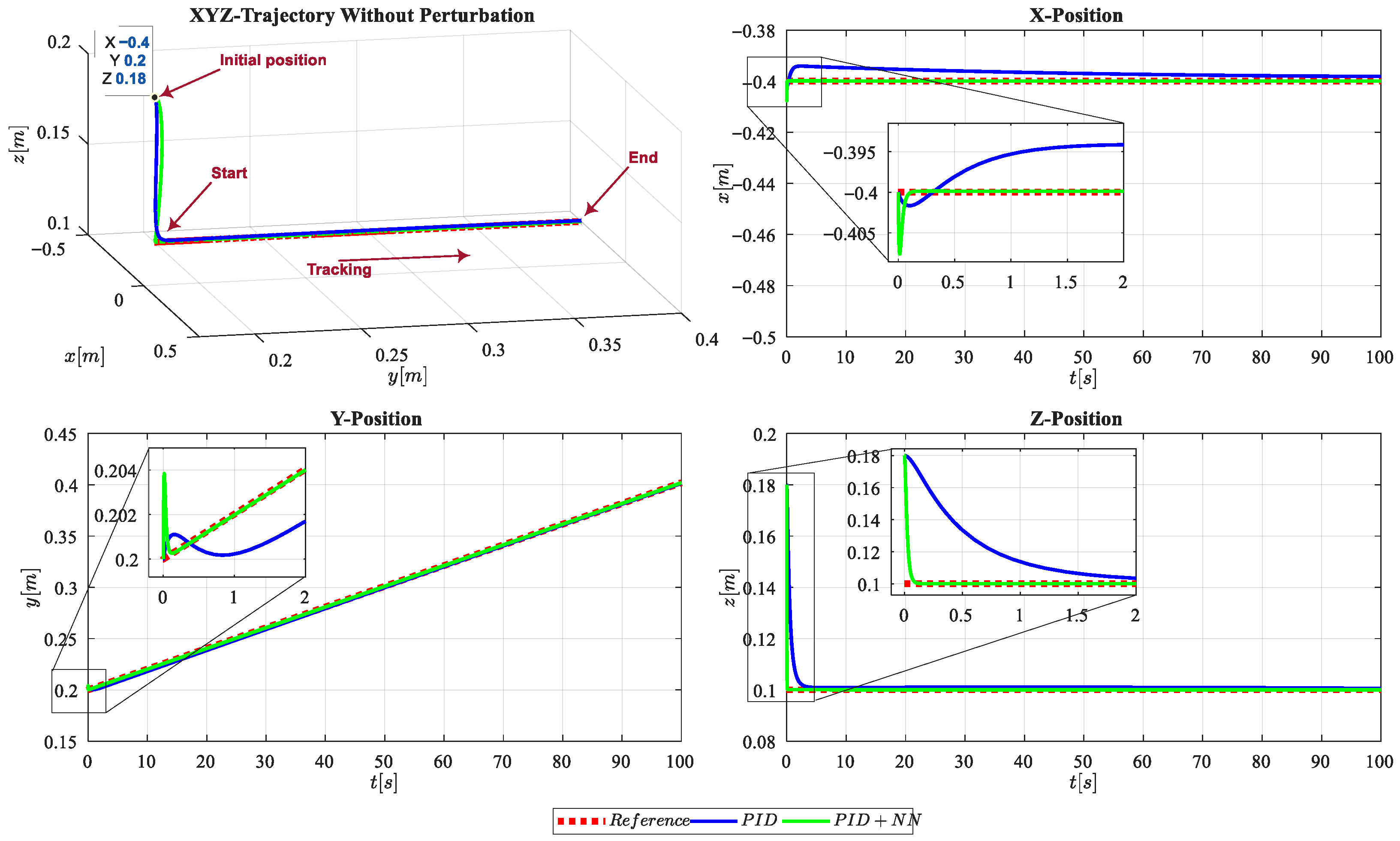
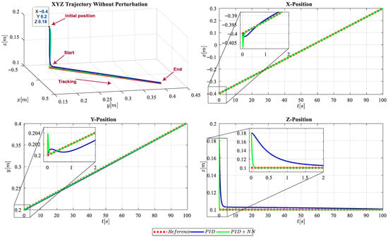
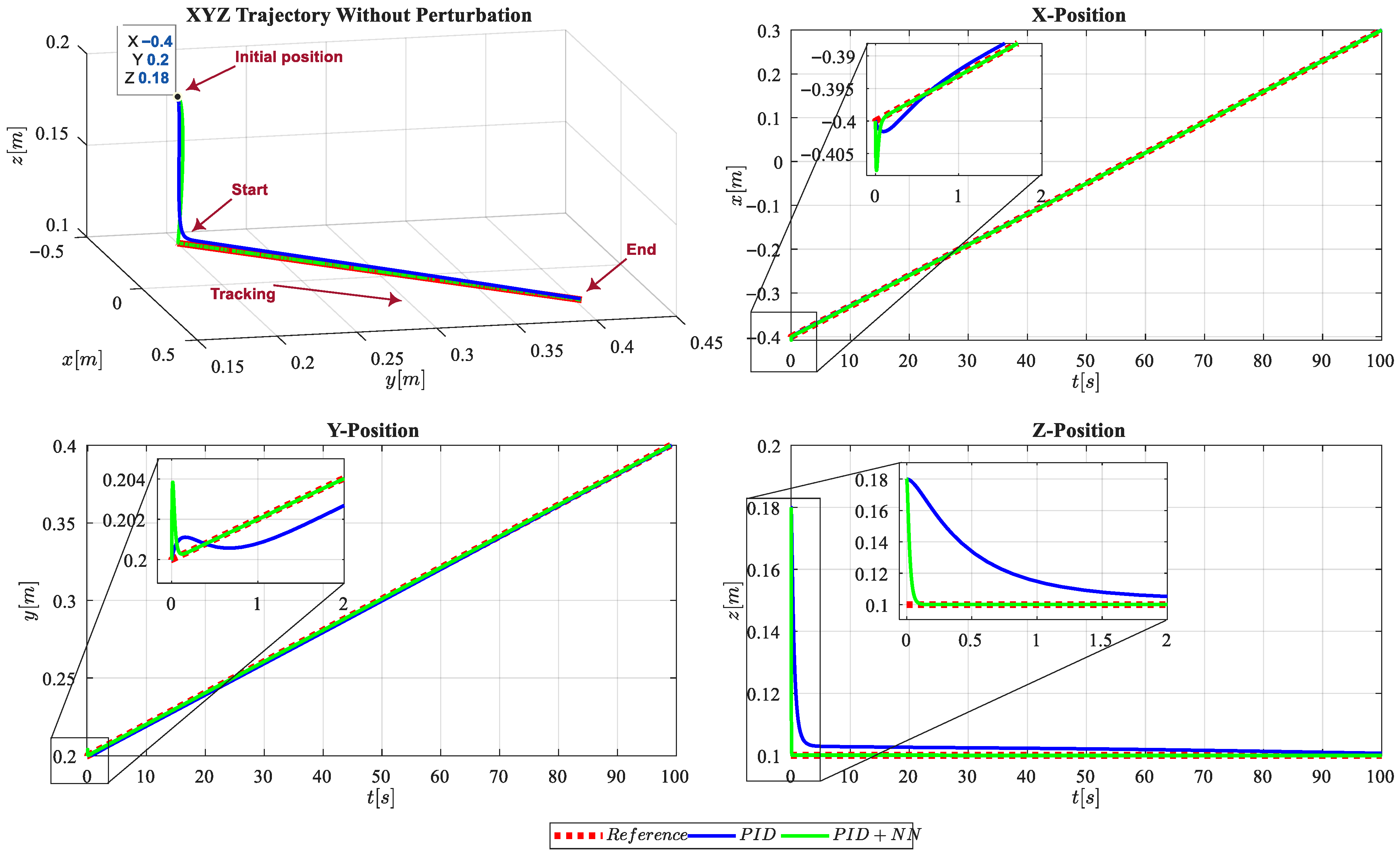
Figure 13. Tracking results for the $L_2$ without perturbation: ideal reference (red dotted line), conventional PID (blue line), and PID + NN (green line).

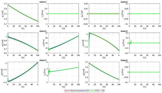
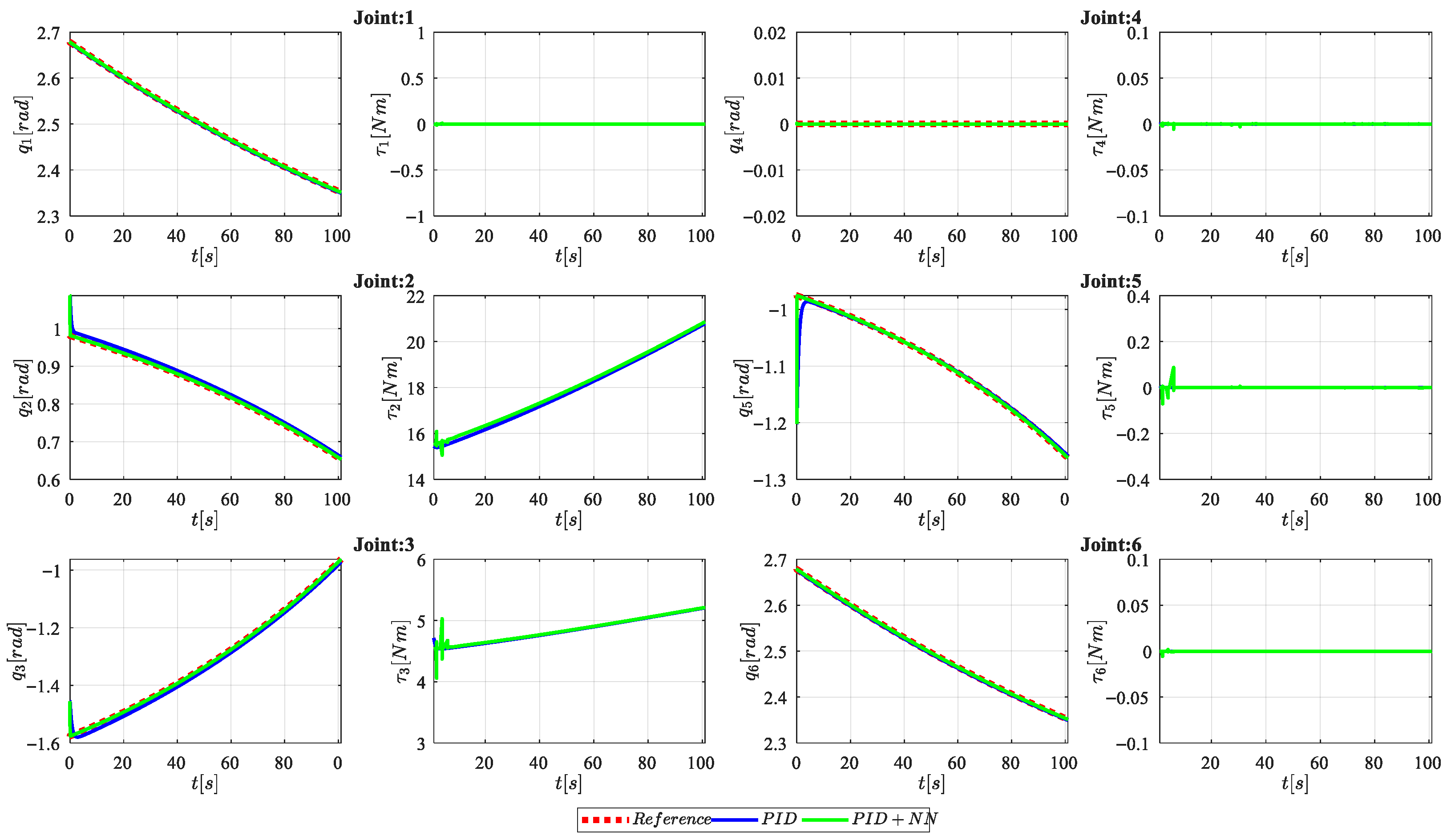
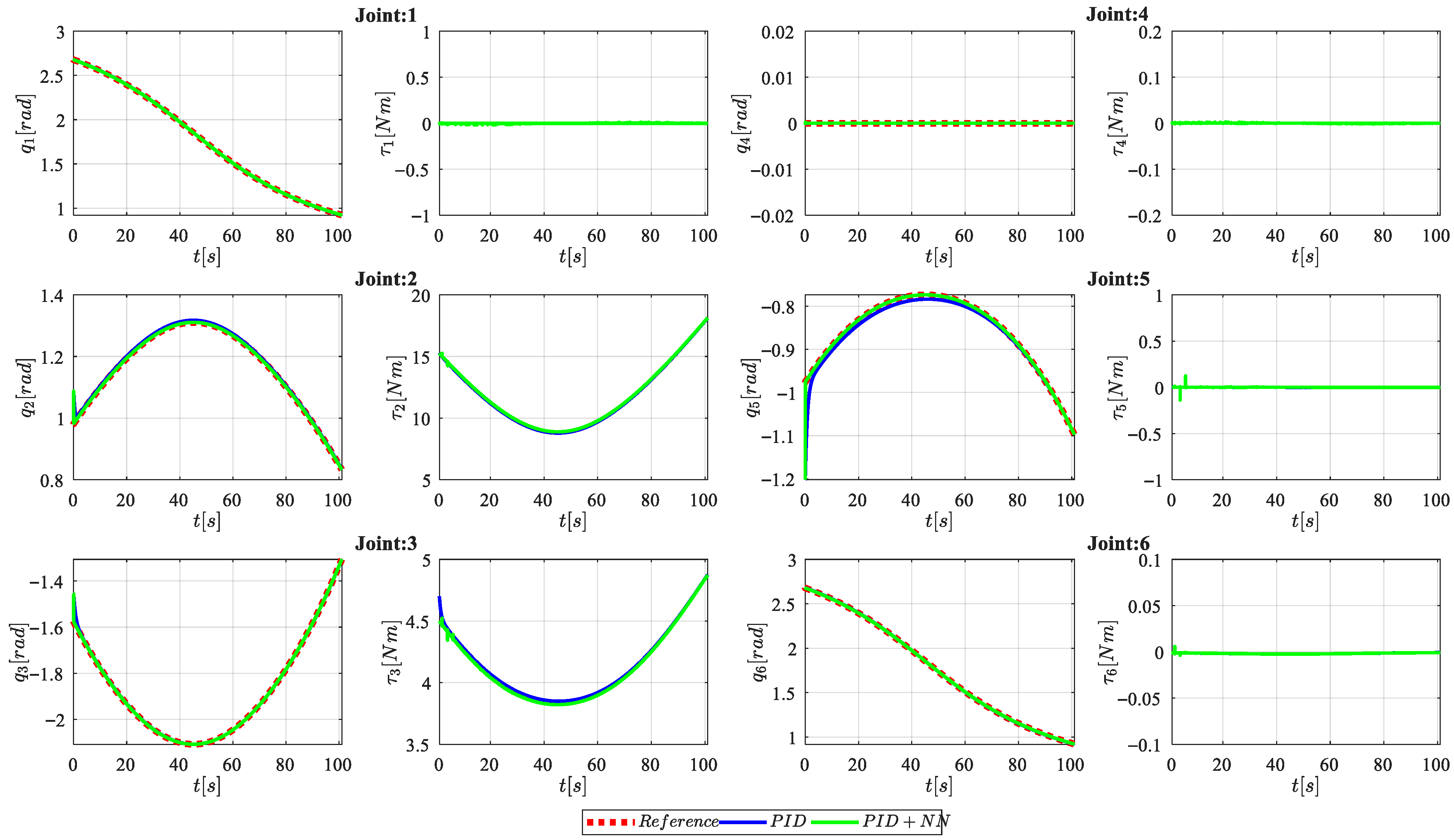
Figure 14. Comparison of angular positions $q_i$ and the control torques ${\tau }_i$ for each joint along the $L_2$ trajectory without perturbation.

Figure 15. Tracking results for the $L_2$ under perturbation: ideal reference (red dotted line), conventional PID (blue line), and PID + NN (green line).

Figure 16. Comparison of angular positions $q_i$ and the control torques ${\tau }_i$ for each joint along the $L_2$ trajectory under perturbation.

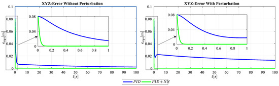
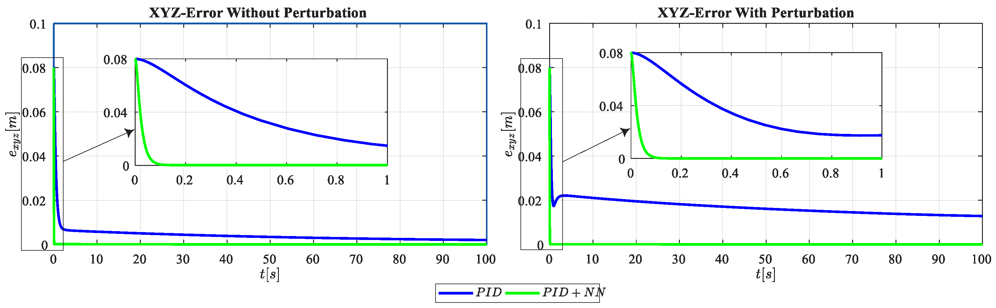
Figure 17. End-effector Cartesian tracking error in Scenario II.

Figure 18. Robot response under nominal conditions for the $L_3$ trajectory: ideal reference (red dotted line), conventional PID (blue line), and PID + NN (green line).

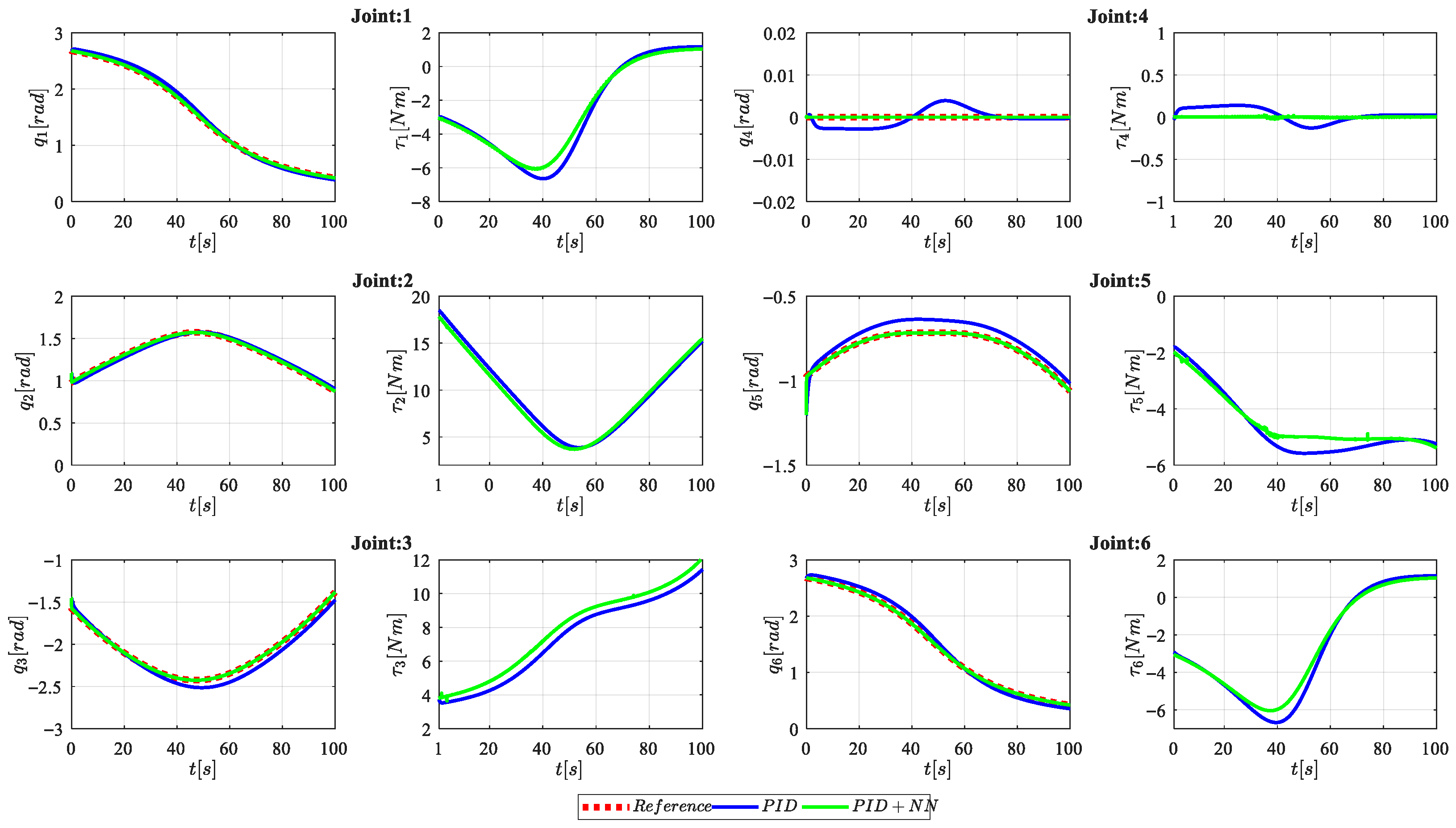
Figure 19. Robot response along the $L_3$ trajectory without perturbation: joint positions $q_i$ and control torques ${\tau }_i$.

Figure 20. Response under perturbation for the $L_3$ trajectory: ideal reference (red dotted line), conventional PID (blue line), and PID + NN (green line).

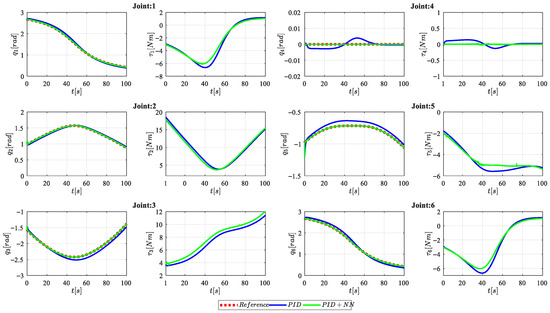
Figure 21. Evolution of joint variables $q_i$ and control torques ${\tau }_i$ along the $L_3$ trajectory with perturbation.

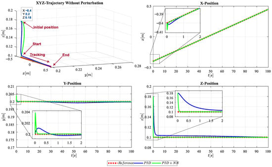
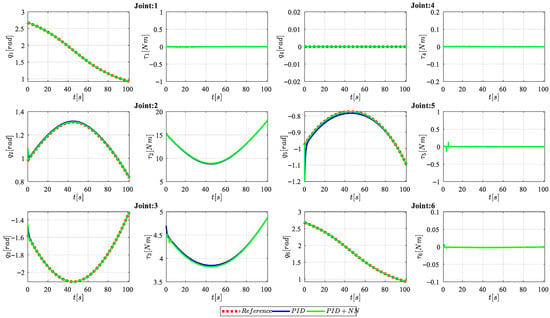
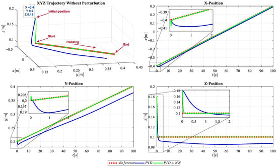
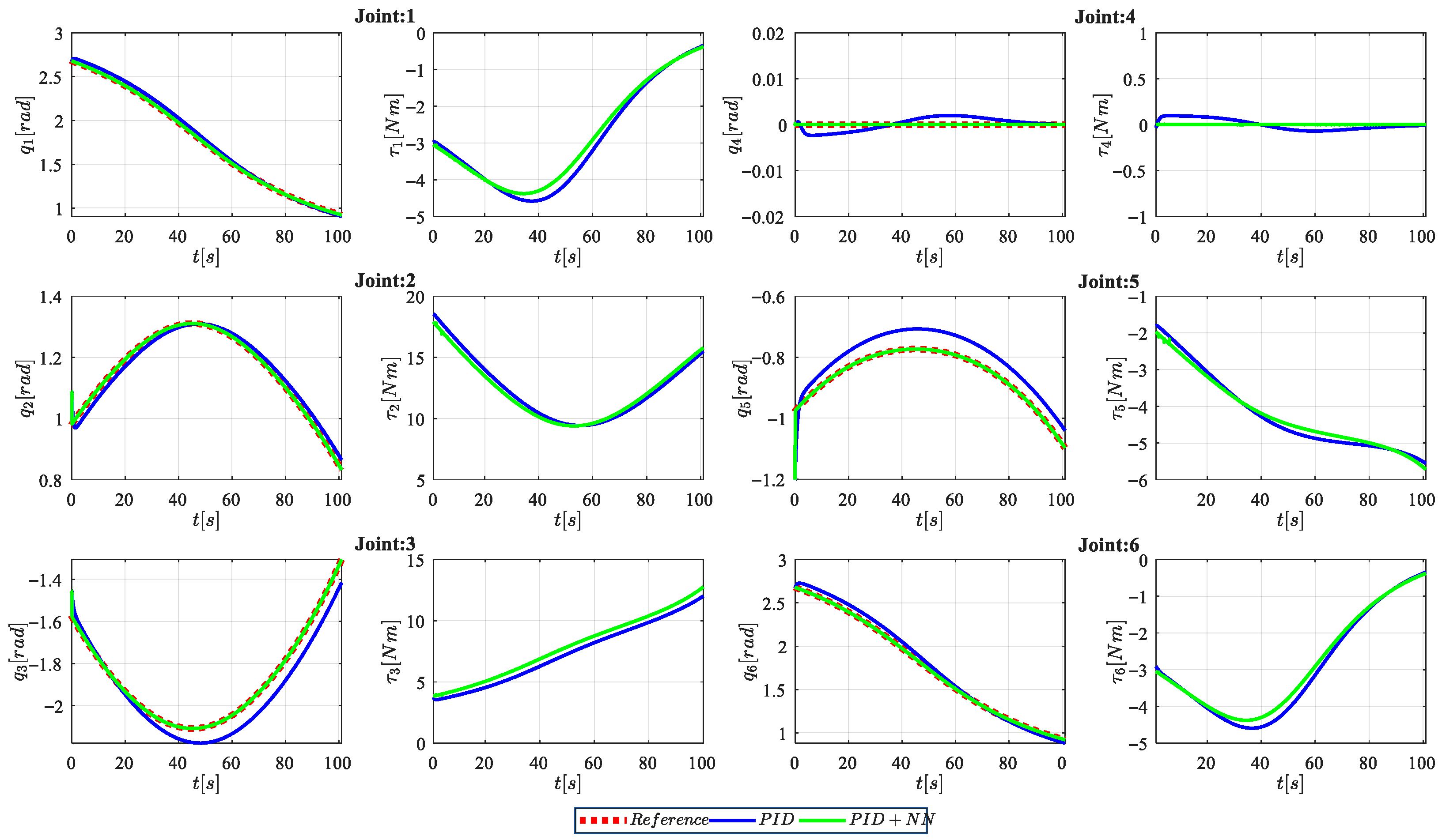
Scenario I. First, Figure 8 and Figure 9 present the results obtained for the system without perturbation. The 3D trajectory shows that the system starts from a distant initial condition and gradually converges toward the reference, with the PID + NN being significantly faster than the conventional PID. On each axis, the classical PID converges more slowly with slight oscillation and overshoot, especially on the y-axis (stabilization time ∼2 s), while the PID + NN almost immediately eliminates the initial error and quickly tracks the reference, demonstrating better dynamic performance. Figure 9 shows the temporal evolution of the control torques at each joint. For both control schemes, the torque signals remain within the linear operating region of the actuators and respect their physical limits, avoiding saturation and possible associated nonlinearities.

Figure 10 and Figure 11 show the results obtained under external perturbation. The classic PID controller exhibits significant transient deviations and a prolonged curved trajectory, demonstrating an intrinsic inability to converge asymptotically to the reference, resulting in a persistent tracking error in steady state. In contrast, the proposed PID + NN hybrid architecture ensures uniform convergence to the equilibrium point through a more direct and smoothed trajectory, even under disturbed initial conditions. This scheme not only minimizes tracking error during the transient phase, but also substantially optimizes perturbation rejection, demonstrating greater robustness and superiority in dynamic performance compared to the inherent limitations of traditional linear control in uncertain environments. Figure 11 shows that the control signals associated with PID + NN exhibit less variability and amplitude of transient peaks compared to conventional PID, which implies a reduction in control effort and potentially less wear on the actuators.

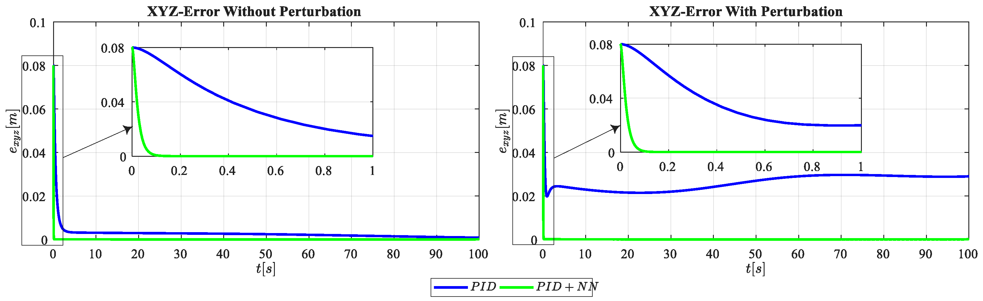
To evaluate performance, Figure 12 illustrates a comparison of the end-effector trajectory tracking error, defined by the following expression:

$$e=\parallel {\mathrm{p}}_r-{\mathrm{p}}_d\parallel$$

(46)

where ${\mathrm{p}}_r$ corresponds to the actual position of the end-effector and ${\mathrm{p}}_d$ to the desired reference position. This comparison allows us to visualize the difference in system performance under both test conditions.

Scenario II. Figure 13 and Figure 14 present the results of the evaluation of the $L_2$ test trajectory without perturbation. It is clearly observed that the classical PID controller suffers from a significant steady-state error and a slower response, being unable to converge accurately to the ideal reference. In contrast, the neural network system manages to correct deviations almost instantaneously, demonstrating greater robustness and tracking accuracy across all three axes (x, y, z). Regarding the angular positions $q_i$ and torques ${\tau }_i$ shown in Figure 14, a smooth and controlled behavior is observed, indicating that the precision added by the neural network does not require excessive mechanical effort nor cause instability in the actuators. Figure 15 and Figure 16 show the results of the evaluation of the test trajectory $L_2$ with perturbation. It is observed that the classic PID cannot maintain its performance with the same gains; that is, it would be necessary to retune it to correct this problem. In contrast, the neural network-based PID algorithm retains its transient characteristics by adapting to the environment while operating within the linear region of the actuators. This represents a significant advantage of the proposed scheme over the classical PID. This demonstrates the effectiveness of artificial intelligence in compensating for nonlinear dynamics or external perturbations that the basic PID cannot handle on its own. Figure 16 shows the positioning of each of the joint positions and pairs.

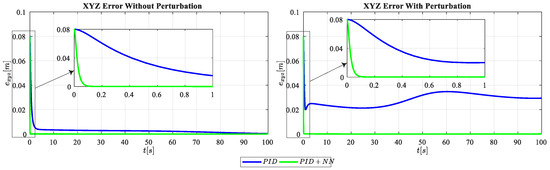
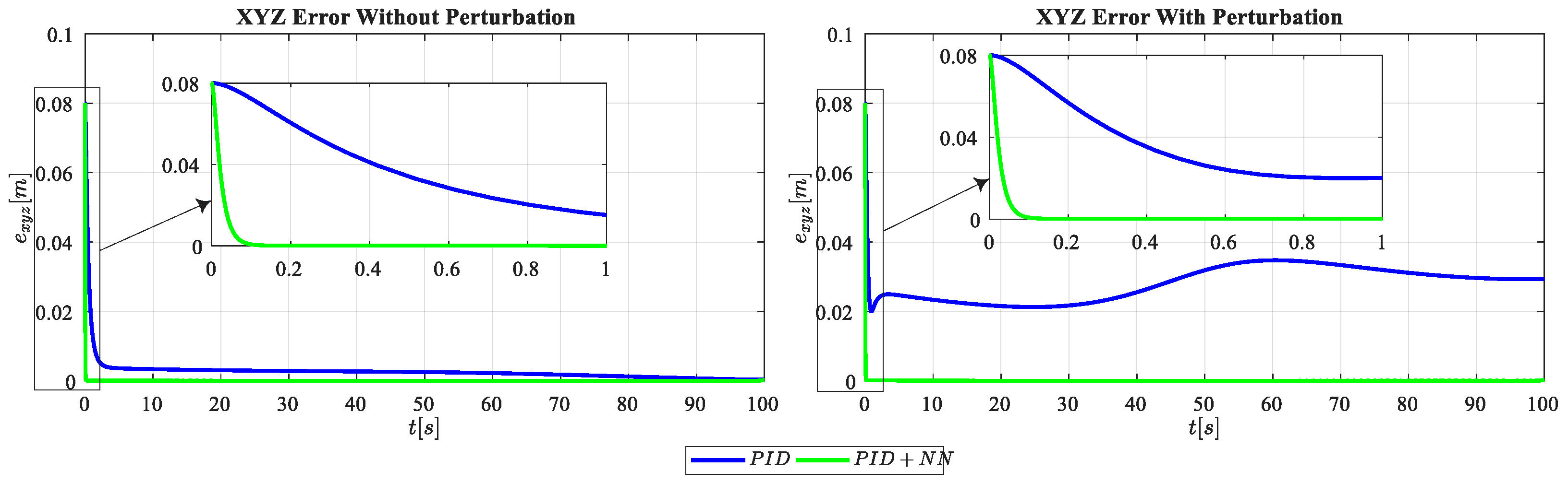
The comparative analysis of the tracking error ($e_{xyz}$) shown in Figure 17 demonstrates that integrating the NN into the PID control scheme significantly improves the robustness and accuracy of the robotic manipulator compared to conventional controllers. While the standard PID controller exhibits slow convergence and a notable degradation in performance in the presence of external perturbations, evidenced by a persistent increase in the residual error, the PID + NN controller achieves effective cancellation of unmodeled dynamics.

Scenario III. This scenario includes the $L_3$ trajectory tracking test; Figure 18, Figure 19, Figure 20, Figure 21 and Figure 22 show the results obtained with and without perturbation. In both tests, the PID + NN scheme maintains the same performance observed in the two previous scenarios: a smooth transient response with a small overshoot, oscillations, or vibrations, and a stabilization time of ∼0.2 s. While the classical PID exhibits a prolonged stabilization time and is unable to eliminate the steady-state error throughout the 100-s test, the neural network-assisted system manages to stabilize in less than 1 s. Finally, the applied torques remain within the saturation limits, where the neural network intelligently compensates for the gravitational loads and the robot’s internal inertia.

Figure 22. End-effector Cartesian tracking error in Scenario III.

For the three scenarios evaluated, the PID + NN hybrid scheme exhibits a smooth dynamic response, characterized by approximately exponential convergence of the error to zero, reduced overshoot, and a gradual transition to steady state. In contrast, the classical PID controller was exhaustively tuned by adjusting its gains with the aim of improving its competitiveness against the proposed approach and avoiding saturation of the control pairs. However, even under the best achievable tuning conditions, the conventional PID failed to simultaneously maintain comparable transient performance and converge accurately to the setpoint. The proposed scheme, on the other hand, consistently achieves both properties.

5. Experimentation

5.1. Platform Experimental Setup

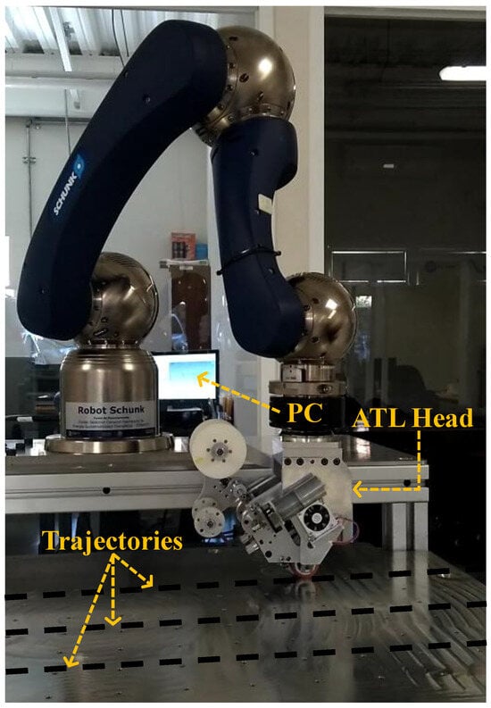
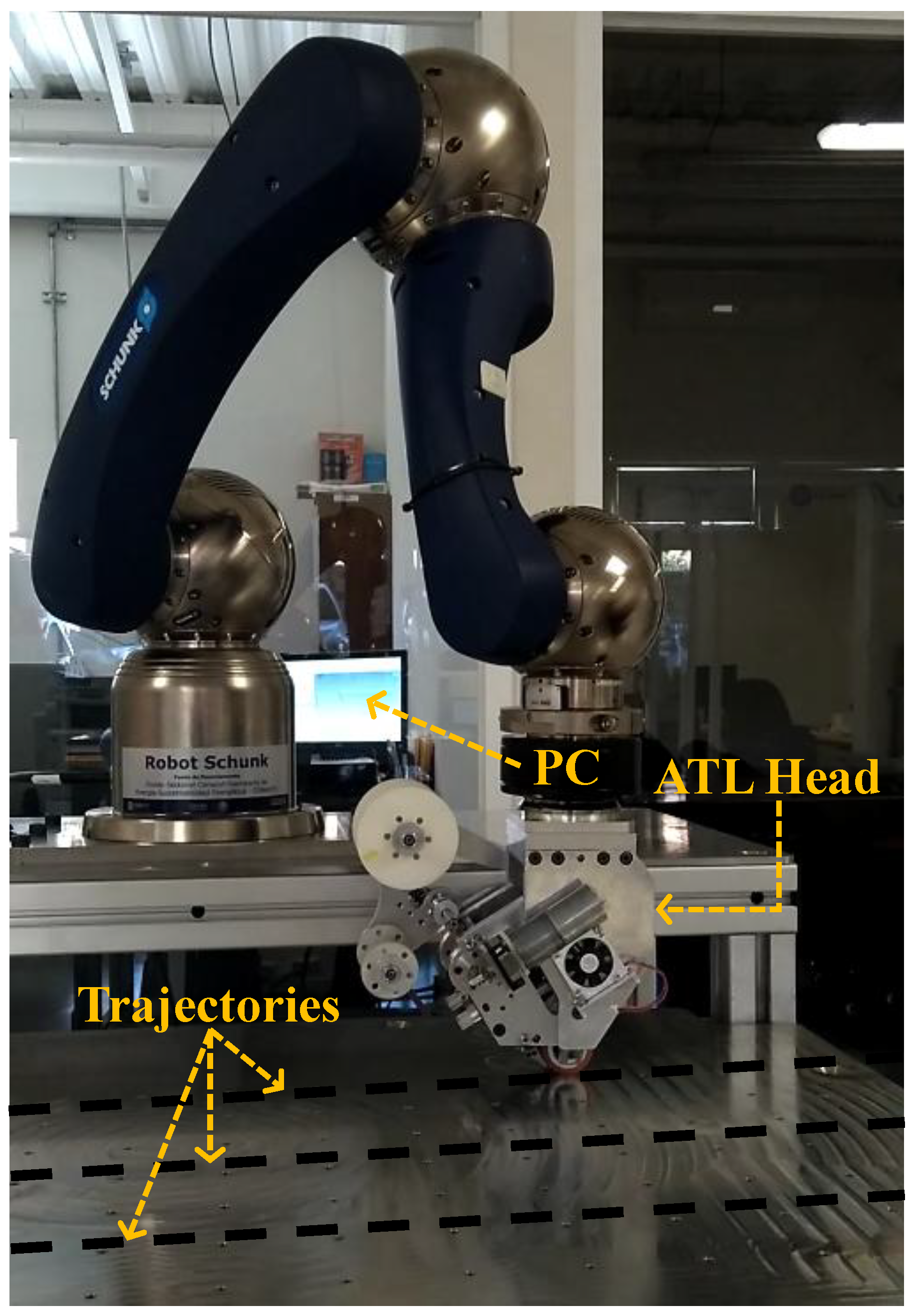
The experimental platform is shown in Figure 23. It uses a SCHUNK Powerball LWA 4P robotic arm, which has 6 DoF. This manipulator stands out for its payload/weight ratio of approximately 1:2.5, with a mass of 15 kg and a nominal load capacity of 6 kg. The mechanical design integrates three Powerball ERB modules equipped with Harmonic Drive reducers and brushless servomotors with permanent magnet braking. In terms of kinematic and dynamic performance, the robot offers a repeatability of ±0.15 mm. Each joint reaches an angular velocity of 72°/s under nominal load, with operating ranges of ±170° (except for link 3, which is limited to ±155.5°). Centralized control is executed on a workstation equipped with an Intel^® Core™ i7-1065G7 (1.30 GHz) processor and 16.0 GB of RAM. Communication with the actuators is established using the CANopen protocol. The control algorithm was developed in the MATLAB/Simulink environment and implemented in the processing unit using automatic code generation techniques (Code Generation Tools). The final effector consists of an ATL head; the main structure uses a 6061 aluminum chassis (3.20 kg), a Nylamid compaction roller (0.15 kg), and transmission systems and motors totaling 1.30 kg, giving a total mass of 4.65 kg. The system’s ATL head moves along a flat surface made of extruded aluminum.

Figure 23. Experimental platform of the robotic arm.

5.2. Results Discusion

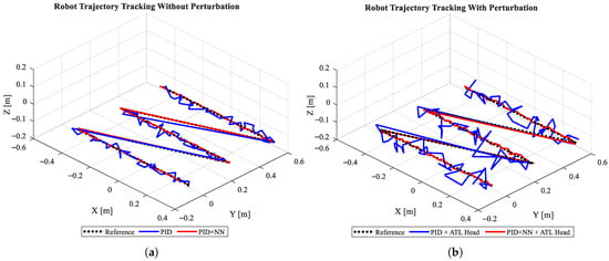
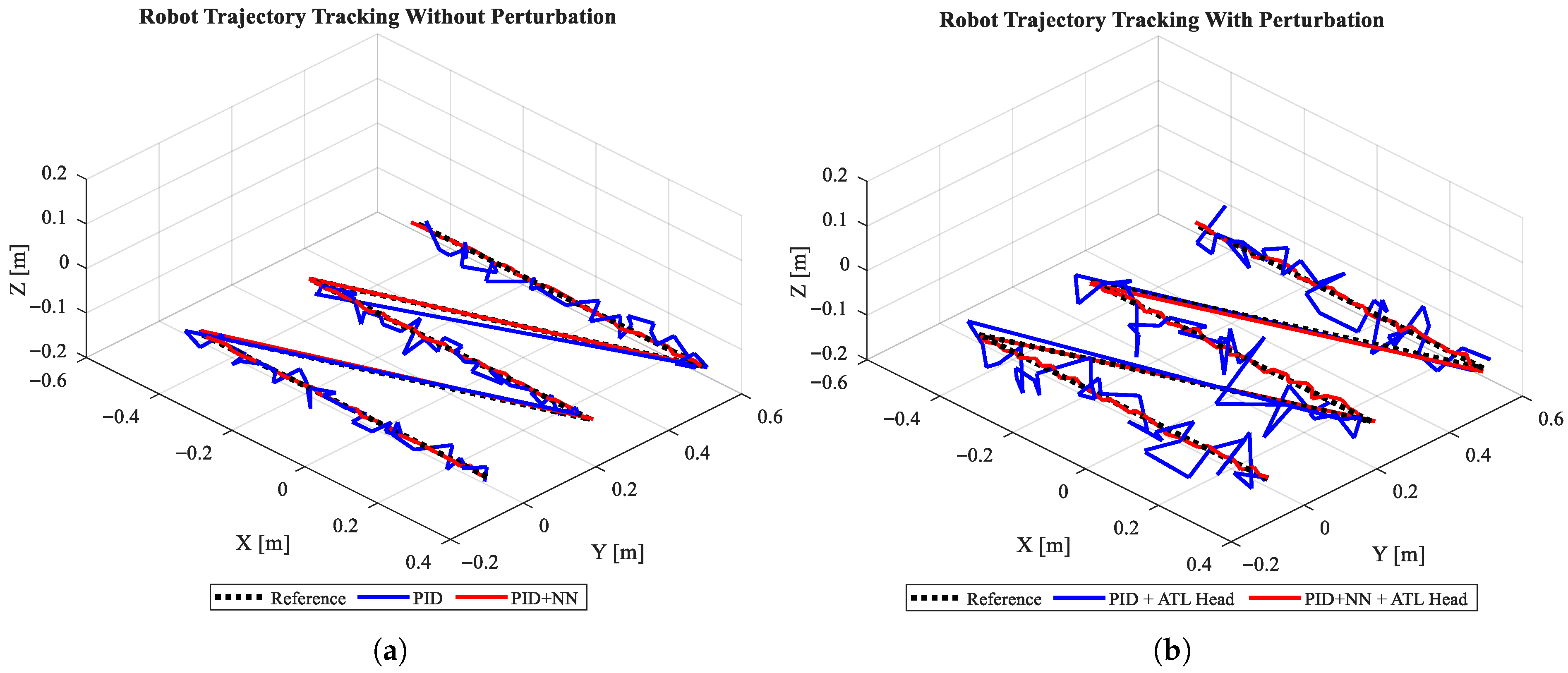
This section presents the real-time experimental results of the two control schemes evaluated: the conventional PID controller and the hybrid PID controller with neural network compensation (PID + NN). Both control strategies were evaluated by tracking three discrete straight-line trajectory segments shown in Figure 23, defined in the task space with variations in the x and y axes, while maintaining a constant altitude of $z=-0.1\mathrm{m}$. This configuration allows the manipulator’s response to reference commands to be analyzed and its spatial stability within the working plane to be evaluated. Figure 24a shows the results obtained under nominal conditions, i.e., when the robot operates without the ATL head. Under these conditions, both controllers manage to converge towards the desired trajectory $P_d$; however, differences in tracking fidelity are observed. The conventional PID controller exhibits persistent dispersion around the reference trajectory, which can be attributed to the limited ability of its fixed linear gains $(K_p,K_i,K_d)$ to fully compensate for measurement noise and unmodeled dynamics present in the system. In contrast, the proposed PID + NN scheme generates a smoother trajectory with less spatial variability, as the neural network acts as an adaptive compensator capable of learning and mitigating the residual error dynamics. This difference becomes more evident when a perturbation in the form of additional load is introduced at the end effector, corresponding to the automated tape placement (ATL) head, which modifies the dynamic conditions of the manipulator. Under these disturbed conditions, the conventional PID controller exhibits more pronounced deviations from the desired trajectory, while the hybrid controller keeps the end effector within a narrow vicinity of the reference, demonstrating greater robustness against load variations in the 6-DOF robotic system, as shown in Figure 24b. To ensure statistical significance, a sampling time of $T_s=0.005\mathrm{s}$ was used over a simulation period of 100 s, resulting in a dataset of approximately 20,000 samples.

Figure 24. Trajectory tracking of the manipulator robot without load (a) and with load (b).

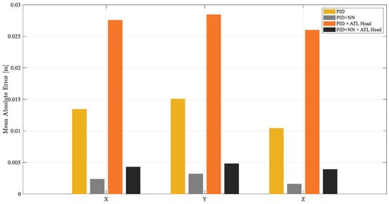
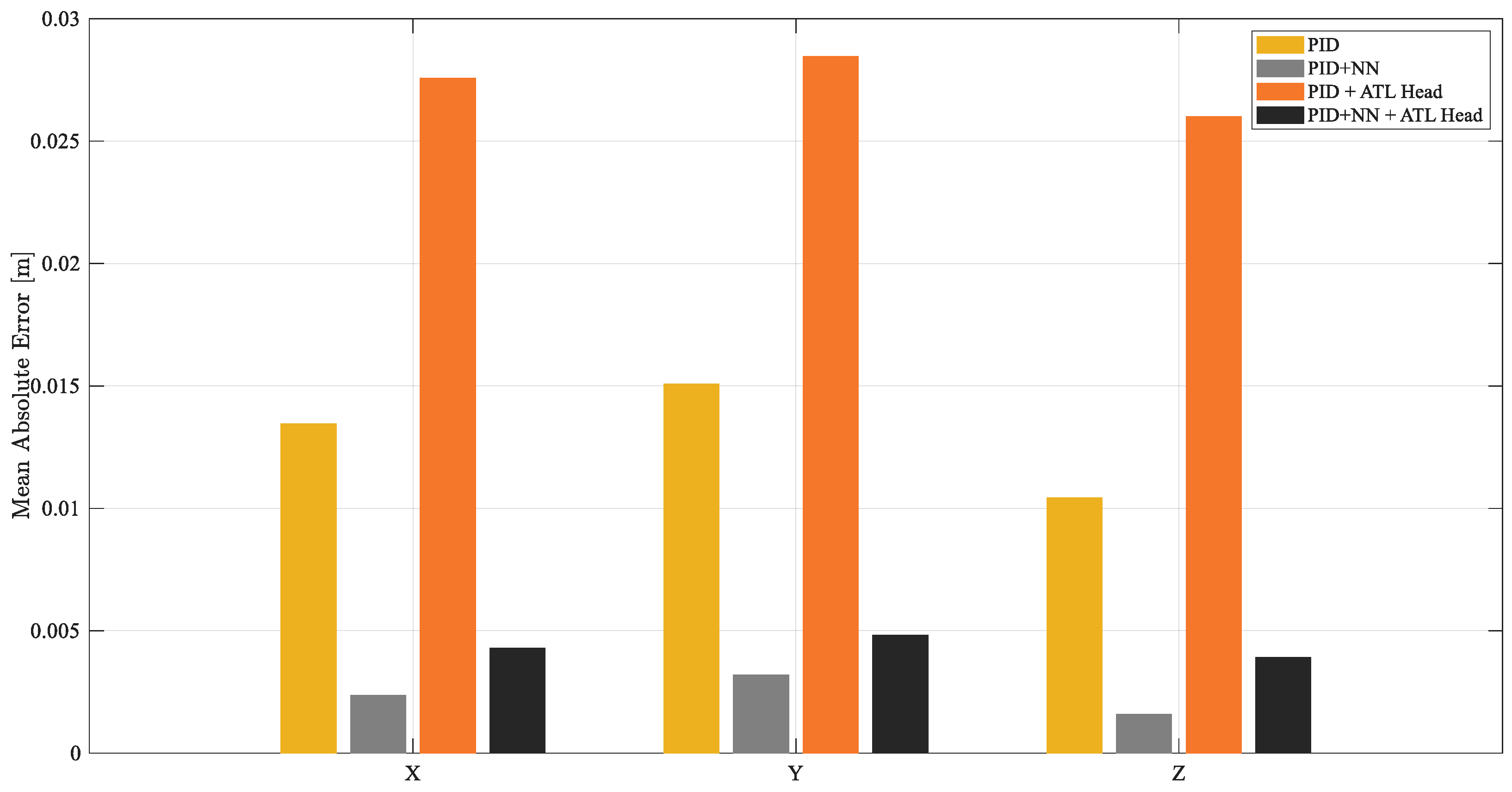
Figure 25 presents the analysis of the average trajectory tracking error on each Cartesian axis. The results show that the hybrid PID + NN scheme consistently reduces the error on the three axes $(x,y,z)$ compared to the conventional PID controller, demonstrating more accurate trajectory tracking. When incorporating an additional load on the end effector using the ATL head, the conventional PID experiences a significant increase in the mean error, reaching values between $0.026$ m and $0.029$ m, which highlights its sensitivity to load variations. In contrast, the PID + NN scheme maintains considerably lower errors, in the order of $0.003$ to $0.005$ m, showing a greater ability to compensate for the dynamic changes associated with the increase in payload. Likewise, the y axis presents the largest errors in both controllers; however, the PID + NN maintains a significant reduction in error compared to the conventional PID.

Figure 25. Box plot of the average trajectory tracking error for the x, y, and z axes.

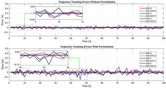
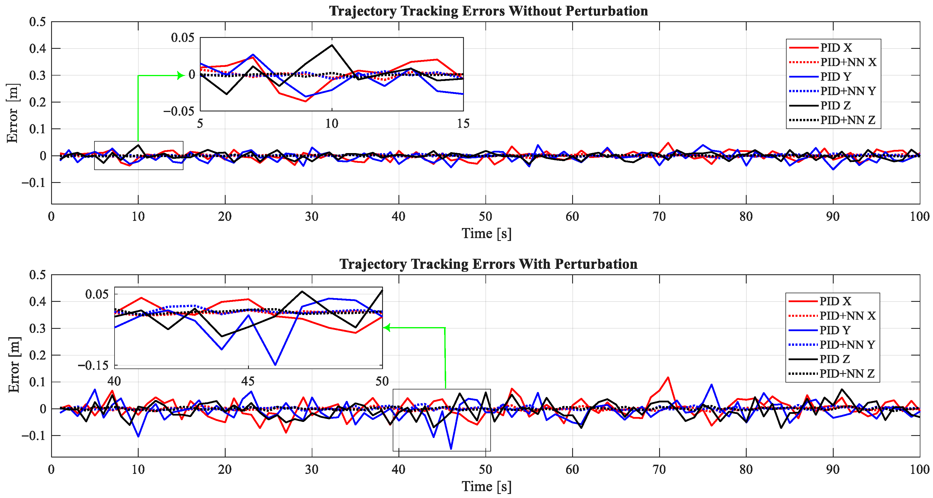
Figure 26 shows the temporal evolution of the trajectory tracking error in the x, y, and z axes, allowing the dynamic behavior of both control schemes to be evaluated under nominal and disturbed conditions. In the absence of load, the conventional PID controller exhibits persistent oscillations around the origin, particularly in the x and y axes, indicating greater error variance. In contrast, the hybrid PID + NN scheme maintains errors of lesser magnitude and with less temporal dispersion, evidencing more stable tracking. When introducing the perturbation associated with the additional load of the ATL head in the end effector, the PID shows a notable increase in the amplitude of the deviations, while the PID + NN maintains an error dynamic close to zero and effectively dampens the transient peaks. Taken together, these results indicate that the hybrid scheme improves perturbation rejection capability and maintains a low tracking error even in the face of variations in the manipulator load.

Figure 26. PID vs. PID + NN trajectory tracking errors separated by perturbation.

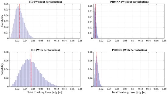
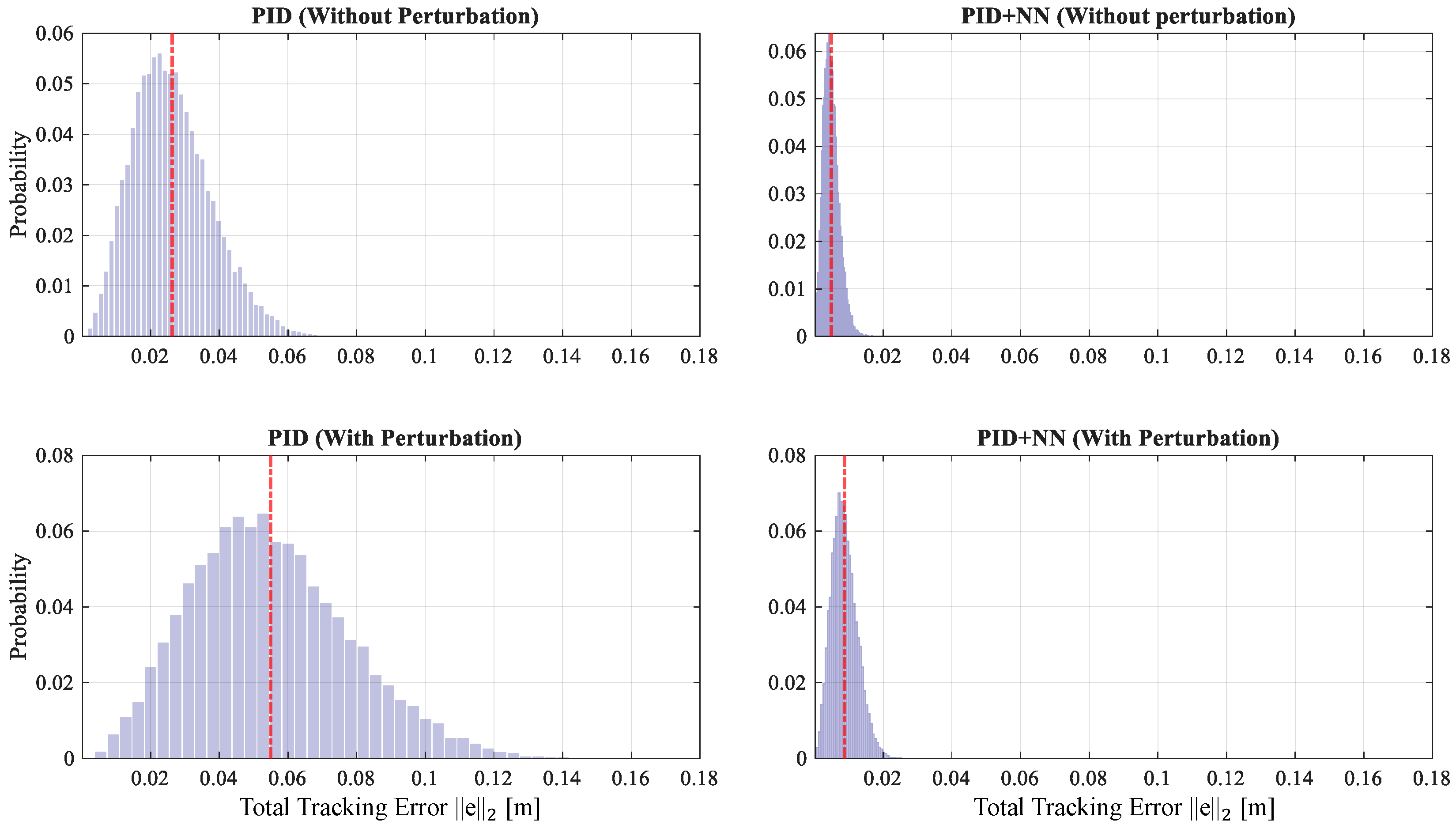
The histograms shown in Figure 27 provide a statistical characterization of the tracking error. These results were obtained using the Euclidean norm ${\parallel e\parallel }_2$, which defines the magnitude of the scalar error in terms of its Cartesian components using the following expression:

$${\parallel e\parallel }_2=\sqrt{e_x^2+e_y^2+e_z^2}$$

(47)

where $e_x$, $e_y$, $e_z$ represent the instantaneous deviations along the x, y, and z axes, respectively [31].

Figure 27. Histograms of the total trajectory tracking error.

A comparative analysis of the tracking error distribution reveals a significant difference in performance between the conventional PID controller and the proposed PID + NN scheme. While the PID exhibits a broad Gaussian distribution, the PID + NN approach produces a high concentration of error near the origin, demonstrating superior accuracy. In the presence of external disturbances, the error distribution in the PID controller undergoes a substantial shift and an increase in variance, with a mean error ${\parallel e\parallel }_2$ rising from approximately $0.02$ m to over $0.05$ m, highlighting the inherent limitations of fixed-gain controllers in the face of dynamic uncertainties. In contrast, analysis of the probability density functions confirms that the PID + NN scheme consistently keeps the error magnitude below $0.02$ m, even under adverse conditions. The high kurtosis of its distribution, compared to the conventional PID, reflects a greater concentration of error around the origin, resulting in a system that is not only more accurate but also more predictable and with reduced fluctuations.

Finally, the control method proposed in this study was compared with various controllers reported in the literature, and the results are summarized in Table 3. Analysis of the data reveals that several authors require a pre-training stage ([23,25,29]) to achieve acceptable levels of accuracy. Although the trajectory tracking error of the proposed controller ($2\mathrm{mm}$) is not the lowest in the comparison, it is important to note that works such as [26], which report significantly smaller errors ($0.1059\mathrm{mm}$), base their results solely on simulations without disturbances. In contrast, the method presented here demonstrates robust and competitive performance in both simulation and real-world experiments without the need for pre-training.

Table 3. Comparative analysis of the proposed controller vs. literature. The symbol “X” denotes a characteristic considered in the study, while “–” denotes characteristics unconsidered.

Reference	Manipulator	Controller	Type of NN	Pre-Training	Sim./Exp.	${\parallel \mathit{e}\parallel }_2$
[22]	5-DOF	NN-PD	MLP	–	X/X	9.62 mm
[23]	2-DOF	NN-Fuzzy	MLP	X	X/–	3.5 mm
[24]	3-DOF	NNKEMFC	FFNN	–	X/–	1.1 mm
[25]	3-DOF	NN-FASA	RBFNN	X	X/–	2.53 mm
[26]	7-DOF	NN	RNN	–	X/–	0.1059 mm
[27]	6-DOF	NN	RBFNN	–	X/X	7 mm
[28]	3-DOF	NN	FFNN	–	X/–	2.8 mm
[29]	6-DOF	NN	CNN	X	–/X	1.27 mm
Proposed method	6-DOF	NN-PID	BP-NN	–	X/X	2 mm

6. Conclusions

This paper presents the development and evaluation of a hybrid control strategy—based on a conventional PID controller supplemented by a neural network—for trajectory tracking in a robotic manipulator used in ATL processes. The stability of the proposed scheme was formally analyzed in the Lyapunov sense, demonstrating that the closed-loop system guarantees stability and keeps tracking errors bounded under the operating conditions considered. To evaluate the controller’s performance, numerical simulations and experimental tests were conducted on a real robotic platform in different scenarios, including variations in the manipulator’s payload. The results show a significant improvement in accuracy when incorporating neural network compensation: while the conventional PID controller exhibited average errors in the range of 26 to 29 mm ($0.026$–$0.029\mathrm{m}$), the hybrid PID + NN scheme reduced these errors to approximately 3 to 5 mm ($0.003$–$0.005\mathrm{m}$). From a practical perspective of the ATL process, considering that the width of the fiber used is 10 mm, the errors of the conventional PID represent deviations of up to 2.9 times the width of the fiber, which would cause critical misalignments, overlaps, or discontinuities in the laminate. In contrast, the hybrid controller keeps the error within $30\%$ to $50\%$ of the fiber width, allowing the end-effector to follow the reference with an acceptable tolerance and reducing the probability of geometric defects. Taken together, these results demonstrate that compensation using neural networks substantially improves the system’s robustness against load variations, positioning this scheme as a promising alternative for high-precision robotic applications in advanced manufacturing.

References

- Cemenska, J.; Rudberg, T.; Henscheid, M. Automated In-Process Inspection System for AFP Machines. SAE Int. J. Aerosp. 2015, 8, 303–309. [Google Scholar] [CrossRef] [Scilit]
- He, K.; Nie, H.; Yan, C. The Intelligent Composite Panels Manufacturing Technology Based on Tape-laying Automatic System. Procedia Cirp 2016, 56, 610–613. [Google Scholar] [CrossRef] [Scilit]
- Denkena, B.; Schmidt, C.; Völtzer, K.; Hocke, T. Thermographic online monitoring system for Automated Fiber Placement processes. Compos. Part B Eng. 2016, 97, 239–243. [Google Scholar] [CrossRef] [Scilit]
- Pantoji, S.; Kassapoglou, C.; Peeters, D. Predicting gaps and overlaps in Automated Fiber Placement composites by measuring sources of manufacturing process variations. Compos. Part B Eng. 2025, 291, 111891. [Google Scholar] [CrossRef] [Scilit]
- Cardoso, D.; Silva, A.R.; Correia, N. Automated Fiber Placement Gap Width Prediction Using a Transformer-Based Deep Learning Approach. Processes 2026, 14, 609. [Google Scholar] [CrossRef] [Scilit]
- Hochster, H.; Raanan, G.; Tiosano, E.; Harari, Y.; Michaeli, G.; Rotbaum, Y.; Haj-Ali, R. Nonlinear Elasticity and Damage Prediction in Automated Fiber Placement Composites via Nested Micromechanics. Materials 2025, 18, 3394. [Google Scholar] [CrossRef] [Scilit]
- Donough, M.J.; Shafaq; St John, N.A.; Philips, A.W.; Prusty, B.G. Process modelling of In-situ consolidated thermoplastic composite by automated fibre placement—A review. Compos. Part Appl. Sci. Manuf. 2022, 163, 107179. [Google Scholar] [CrossRef] [Scilit]
- Yadav, N.; Schledjewski, R. Review of in-process defect monitoring for automated tape laying. Compos. Part Appl. Sci. Manuf. 2023, 173, 107654. [Google Scholar] [CrossRef] [Scilit]
- Özbilgin, F.; Mengi, O.Ö.; Wadood, A.; Güven, A.F.; Park, H. Comparative optimization of PIDN and fractional order controllers for a quarter car active suspension system using recent metaheuristic algorithms. Sci. Rep. 2025, 15, 35222. [Google Scholar] [CrossRef] [Scilit]
- Çelik, D.; Khosravi, N.; Khan, M.A.; Waseem, M.; Ahmed, H. Advancements in nonlinear PID controllers: A comprehensive review. Comput. Electr. Eng. 2026, 129, 110775. [Google Scholar] [CrossRef] [Scilit]
- Blanco Rico, J.; Reyes-Cortes, F.; Al-Hadithi, B.M. A New Hyperbolic PID-Type Control Scheme for a Direct-Drive Pendulum. Electronics 2026, 15, 942. [Google Scholar] [CrossRef] [Scilit]
- Chen, Z.; Wen, W.; Yang, W. Adaptive Visual Control for Robotic Manipulators with Consideration of Rigid-Body Dynamics and Joint-Motor Dynamics. Mathematics 2024, 12, 2413. [Google Scholar] [CrossRef] [Scilit]
- Duan, J.; Gan, Y.; Chen, M.; Dai, X. Symmetrical adaptive variable admittance control for position/force tracking of dual-arm cooperative manipulators with unknown trajectory deviations. Robot. Comput.-Integr. Manuf. 2019, 57, 357–369. [Google Scholar] [CrossRef] [Scilit]
- Jankowski, K.P.; ElMaraghy, H.A. Robust hybrid position/force control of redundant robots. Robot. Auton. Syst. 1999, 27, 111–127. [Google Scholar] [CrossRef] [Scilit]
- Solanes, J.E.; Gracia, L.; Muñoz-Benavent, P.; Esparza, A.; Valls Miro, J.; Tornero, J. Adaptive robust control and admittance control for contact-driven robotic surface conditioning. Robot. Comput.-Integr. Manuf. 2018, 54, 115–132. [Google Scholar] [CrossRef] [Scilit]
- Long, J.; Tian, Y.; Chen, W.; Leng, J.; Wang, Y. Locating, trajectory planning and control of an underwater propeller cleaning manipulator. Ocean Eng. 2022, 243, 110262. [Google Scholar] [CrossRef] [Scilit]
- Gutiérrez-Giles, A.; Arteaga-Pérez, M.A.; Sira-Ramírez, H. Control de Fuerza de Robots Manipuladores Basado en Observadores Proporcionales Integrales Generalizados. Rev. Iberoam. Automática Informática Ind. Riai 2016, 13, 238–246. [Google Scholar] [CrossRef] [Scilit]
- Zaare, S.; Soltanpour, M.R. Uncertainty and velocity observer-based predefined-time nonsingular terminal sliding mode control of the underwater robot manipulators. Eur. J. Control 2024, 75, 100939. [Google Scholar] [CrossRef] [Scilit]
- Cao, P.; Gan, Y.; Dai, X. Finite-Time Disturbance Observer for Robotic Manipulators. Sensors 2019, 19, 1943. [Google Scholar] [CrossRef] [Scilit]
- Huang, Y.; Li, W.; Cui, Z.; Hu, Y.; Li, Z. An Adaptive Finite-Time Convergent Neural Network with Enhanced Joint Limit Constraints for 3-DoF Visual Servoing of Rigid-Flexible Coupling Robots. IEEE Trans. Ind. Electron. 2026, 1–13. [Google Scholar] [CrossRef] [Scilit]
- Qin, Y.; Sun, Y.; Huang, J.; Li, Y. Adaptive Predefined-Time Tracking Control for Robotic Manipulator Based on Actor-Critic Reinforcement Learning. Sensors 2026, 26, 1529. [Google Scholar] [CrossRef] [Scilit]
- Hernandez-Barragan, J.; Rios, J.D.; Gomez-Avila, J.; Arana-Daniel, N.; Lopez-Franco, C.; Alanis, A.Y. Adaptive neural PD controllers for mobile manipulator trajectory tracking. Peerj Comput. Sci. 2021, 7, e393. [Google Scholar] [CrossRef] [Scilit]
- Shen, Y. Robotic trajectory tracking control system based on fuzzy neural network. Meas. Sens. 2024, 31, 101006. [Google Scholar] [CrossRef] [Scilit]
- Hancioğlu, O.K.; Efe, M.Ö. Neural Network Augmented Koopman Explicit Model Following Control for Robotic Manipulators. IEEE Access 2026, 14, 24330–24338. [Google Scholar] [CrossRef] [Scilit]
- Xu, J.; Zhang, K.; Ning, Z.; Chen, Z. Neural network-based fully actuated trajectory tracking control for space manipulator with system uncertainties. Neurocomputing 2025, 647, 130399. [Google Scholar] [CrossRef] [Scilit]
- Li, J.; Su, J.; Yu, W.; Mao, X.; Liu, Z.; Fu, H. Recurrent neural network for trajectory tracking control of manipulator with unknown mass matrix. Front. Neurorobot. 2024, 18, 1451924. [Google Scholar] [CrossRef] [Scilit]
- Song, Q.; Li, S.; Bai, Q.; Yang, J.; Zhang, A.; Zhang, X.; Zhe, L. Trajectory planning of robot manipulator based on RBF neural network. Entropy 2021, 23, 1207. [Google Scholar] [CrossRef] [Scilit]
- Kumar, N.; Panwar, V.; Sukavanam, N.; Sharma, S.P.; Borm, J.H. Neural network-based nonlinear tracking control of kinematically redundant robot manipulators. Math. Comput. Model. 2011, 53, 1889–1901. [Google Scholar] [CrossRef] [Scilit]
- Zhao, X. Adaptive robotic arm control through digital twin integration and hybrid neural networks. Sci. Rep. 2026, 16, 4988. [Google Scholar] [CrossRef] [Scilit]
- Kelly, R.; Santibañez, V.; Loria, A. Control of Robot Manipulators in Joint Space; Springer: London, UK, 2005. [Google Scholar]
- Reyes Cortés, F.; Rodríguez Cruz, F.J. Robótica: Control de Robots Manipuladores; Alfaomega: Ciudad de México, México, 2011. [Google Scholar]
- Lewis, F.L.; Dawson, D.M.; Abdallah, C.T. Robot Manipulator Control: Theory and Practice; CRC Press: Boca Raton, FL, USA, 2003. [Google Scholar]
- Ponce, A.N.; Behar, A.A.; Hernández, A.O.; Sitar, V.R. Neural Networks for Self-tuning Control Systems. Acta Polytech. 2004, 44, 1. [Google Scholar] [CrossRef] [Scilit]
- Memar, A.H.; Esfahani, E.T. Modeling and Dynamic Parameter Identification of the SCHUNK Powerball Robotic Arm. In Proceedings of the ASME 2015 International Design Engineering Technical Conferences and Computers and Information in Engineering Conference; American Society of Mechanical Engineers (ASME): New York, NY, USA, 2015; Volume 5C, p. V05CT08A024. [Google Scholar] [CrossRef] [Scilit]
- SCHUNK GmbH & Co. KG. Assembly and Operating Manual: LWA 4P Powerball Lightweight Arm. In Technical Manual, Version 04.00; SCHUNK GmbH & Co. KG: Lauffen am Neckar, Germany, 2018; p. 1344817. Available online: https://www.schunk.com (accessed on 15 February 2026).
Disclaimer/Publisher’s Note: The statements, opinions and data contained in all publications are solely those of the individual author(s) and contributor(s) and not of MDPI and/or the editor(s). MDPI and/or the editor(s) disclaim responsibility for any injury to people or property resulting from any ideas, methods, instructions or products referred to in the content. |
© 2026 by the authors. Published by MDPI on behalf of the International Institute of Knowledge Innovation and Invention. Licensee MDPI, Basel, Switzerland. This article is an open access article distributed under the terms and conditions of the Creative Commons Attribution (CC BY) license.