Optimized Lyapunov-Theory-Based Filter for MIMO Time-Varying Uncertain Nonlinear Systems with Measurement Noises Using Multi-Dimensional Taylor Network

Abstract

Minimizing the impacts of coupling, randomness, time variation and uncertain nonlinearity to enhance real-time performance is critical for controlling complex industrial systems. This paper proposes an optimized adaptive filtering method (LAF-MTNF) for time-varying uncertain nonlinear systems with multiple-input multiple-output (MIMO) measurement noise, which integrates the multi-dimensional Taylor network (MTN) with Lyapunov stability theory (LST). Leveraging MTN’s inherent advantages—simple structure, linear parameterization, and low computational complexity—LAF-MTNF achieves efficient real-time filtering while avoiding the exponential computation burden of neural networks. The contributions of this work are threefold: (1) A novel integration of LST and MTN is proposed for MIMO filtering, in which an energy space is constructed with a unique global minimum to eliminate local optimization traps, addressing the stability deficit of traditional MTN filters using LMS/RLS algorithms. (2) Convergence performance is systematically quantified by deriving explicit expressions for the error convergence rate (regulated by a positive constant) and convergence region (a sphere centered at the origin) while modifying adaptive gain to avoid singularity, filling the gap of incomplete performance analysis in existing Lyapunov-based filters. (3) The design is disturbance-independent, relying only on input/output measurements and requiring no prior knowledge of noise statistics, thus enhancing robustness to unknown industrial disturbances. We systematically analyze the Lyapunov stability of LAF-MTNF, and simulations on a complex MIMO system verify that it outperforms existing methods in filtering precision (mean error 0.0227 vs. 0.0674 of RBFNN) and dynamic response speed, while ensuring asymptotic stability and real-time applicability. The proposed LAF-MTNF method achieves significant advantages over traditional adaptive filtering methods in filtering accuracy, convergence speed and anti-cross-coupling capability. This method has broad application prospects in high-precision industrial servo motion control, power system state monitoring and other multi-variable nonlinear industrial scenarios with complex noise environments.

1. Introduction

In industrial fields, controlled systems are usually characterized by uncertainty, strong coupling, substantial nonlinearity, distinct time variance and measurement noise. It is hard to secure precise control even with intelligent control methods, such as adaptive control [1,2,3], fuzzy control [4,5,6], neural network control [7,8], and decoupling control [9,10]. As a result, a number of mixed control methods have been developed, including the multi-dimensional Taylor network (MTN). MTN has been applied in system identification [11], motor control [12], adaptive control and nonlinear control [13], leveraging its self-learning, self-organizing, and self-adaptive capabilities to automatically identify and adjust controlled system parameters. However, existing MTN-based filtering methods (e.g., those using least mean square (LMS) or recursive least squares (RLS) for weight updates) face two critical limitations: (1) The optimization process is prone to trapping local minima of the cost function, especially when initial weights are randomly selected. (2) Stability cannot be guaranteed under strong coupling or time-varying disturbances, as LMS/RLS lack a theoretical framework for stability verification. To address these gaps, we propose an adaptive MTN filter (MTNF) that integrates Lyapunov stability theory (LST) to optimize weight updates and ensure system stability. Through the adaptive tuning of MTNF weights, the Lyapunov function is employed to build an energy surface that features a single global minimum. By selecting the weights update rule to be appropriate for Lyapunov filtering, the outputs of the MTNF can converge exponentially to the desired signal. This design is independent of the random characteristics of the input disturbance.

Denoising measurement data in modern industrial control is known to be indispensable for analyzing and controlling industrial processes [14,15]. The result of denoising treatment will directly affect the signal-based fault analysis and diagnosis, object identification, modeling, control process optimization and other functions. If not addressed, measurement noise and random disturbances will inevitably appear at the input of the feedforward controller without being suppressed. This will seriously affect the stability and control accuracy of the adaptive process. More importantly, it has been established that feedback accuracy sets a ceiling for control accuracy, meaning that the latter cannot go beyond the former. However, input and output data are usually affected to varying degrees by various forms of noise, and to date, existing research methods cannot completely eliminate the impact of noise on control accuracy. Therefore, we need to minimize the influence of noise on the useful signal as much as possible.

Currently, it is widely believed that objects in industrial processes are complex, nonlinear, time-varying systems in which system noise and observation noise also vary over time [16,17]. In modern control systems, fixed low-pass filters are typically used to remove high-frequency interference from the system in order to deal with this noise and interference. However, the filtering parameters remain constant throughout the denoising process. This makes the denoising algorithm unsuitable for time-varying systems and prone to overshoot. This can lead to uneven filter output and even severely impact the performance of the control system.

For high-precision industrial robotics and micromachining scenarios, conventional adaptive filters face an insurmountable performance ceiling: non-stationary noise from mechanical vibration and dynamic working condition changes will cause steady-state bias or even divergence of traditional methods, which cannot meet the nanometer-level positioning accuracy requirements [18,19]. The MTN architecture, with its strong nonlinear approximation capability and Lyapunov-guaranteed stability under bounded non-stationary noise, provides a necessary solution to this industrial pain point. Using a linear weighting combiner, the weights of the MTNF can be adjusted using the LMS and RLS algorithms. However, these algorithms have some limitations and drawbacks [20]. To avoid instability, designers had to seek other solutions. Moreover, should the initial value be chosen arbitrarily, the optimization search could halt at a local minimum within the parameter space of the cost function. If the interference encountered by the filter is a random signal, then mathematical methods for random processes must be used for optimization and parameter design.

LST has been widely used in adaptive filtering to guarantee stability and construct energy spaces with global minima. Our group has conducted pioneering research on MTN-based adaptive filtering for nonlinear systems. In [13], a basic MIMO MTNF framework combined with Lyapunov-based adaptive filtering (LAF) was first proposed, which achieved basic measurement noise elimination for MIMO time-varying systems and proved the asymptotic convergence of the filtering error. However, the existing work only regards MTNF as an auxiliary noise elimination module matched with the tracking controller, and has not established an independent and complete adaptive prediction filtering theoretical system for strongly coupled, high-dimensional industrial MIMO systems. Meanwhile, there are still research gaps in the quantitative characterization of convergence performance, strict proof of global optimality, high-dimensional scalability design, and robustness analysis for industrial non-ideal correlated noise. Built on the above pioneering work, this paper systematically deepens the LAF-MTNF theoretical framework, and proposes a dedicated adaptive prediction filtering scheme for complex industrial MIMO systems with strong coupling, high dimensionality and complex measurement noise. Compared with the quadratic cost function of traditional LMS/RLS filters, which only has a global minimum under ideal linear system and white noise assumptions and is prone to local optimization traps in nonlinear MIMO systems with non-ideal noise [21], the Lyapunov function-based weight update law in this paper strictly follows the global asymptotic stability criteria [22]. It guarantees that the filtering error asymptotically converges to zero, and the network weights converge to the unique global optimal solution, fundamentally eliminating local optimization traps without the need for complex initial value selection. For example, LST-based RBF neural networks (RBFNN) have been applied to finite-impulse response (FIR) and infinite-impulse response (IIR) adaptive filters [23], but they suffer from a key limitation: the selection of RBF node centers and Gaussian widths lacks an effective optimization algorithm, leading to suboptimal filtering performance. More importantly, two critical research gaps persist in LST-based filtering: (1) Few studies have integrated LST with MTN for filtering—despite MTN’s advantages of simple structure and linear parameterization, no work has used LST to solve MTN’s weight update instability. (2) Existing Lyapunov filtering research has only provided basic stability verification, and the convergence rate and convergence region of filters with corrected gains (to avoid singularity) have not been systematically analyzed. These gaps make it difficult for existing methods to handle MIMO time-varying uncertain nonlinear systems with strong coupling and measurement noise.

The MTN’s advantages of arbitrary approximation capability and simple linear-parameter computation (via weighted intermediate layer nodes) make it a promising candidate for nonlinear system filtering. A supplementary core objective of this work is to optimize the computational scalability of the LAF-MTNF architecture in high-dimensional MIMO systems (with 3 or more inputs/outputs), addressing the rapid growth of Taylor expansion terms while balancing approximation accuracy and real-time performance. For an MTN with n input variables and maximum expansion order m, the total number of polynomial terms is $N(n,m)=(n+m)!/(n!m!)$, which follows a polynomial growth trend with the increase in system dimensions. This work adopts a low-order expansion strategy (typically $m = 2$ or $m=3$, which is sufficient for most industrial nonlinear systems) and a sparse term pruning mechanism to suppress term number growth, ensuring computational efficiency in high-dimensional scenarios. The proposed method can be directly applied to typical industrial scenarios with high requirements for filtering accuracy, real-time performance and stability, and the core contributions of this work are summarized as follows: (1) Novel Integration of LST and MTN for MIMO Filtering: We propose the first LST-based adaptive IIR filter using MTN (LAF-MTNF) for MIMO time-varying uncertain nonlinear systems. Unlike existing MTNF with LMS/RLS weight updating [11], our LST-based weight adaptation algorithm eliminates local minima and guarantees global stability by constructing an energy space with a single global minimum. (2) Systematic Analysis of Convergence Rate and Region: We address the unexamined issue of singularity avoidance and convergence performance in Lyapunov filtering; by modifying the adaptive gain, we derive explicit mathematical expressions for the error convergence rate (related to the positive constant (Equation (12)) and convergence region (a sphere centered at the origin with radius defined in Equation (14)), filling the gap of incomplete performance analysis in existing work [24]. (3) Disturbance-Independent Design: The proposed LAF-MTNF only relies on input/output measurements and does not require prior knowledge of the random characteristics of input disturbances (e.g., measurement noise statistics). This is a key advantage over existing adaptive filters that depend on noise distribution assumptions [25,26]. Specifically, we integrate LST into MTN’s supervised training by defining a Lyapunov function $V$ (energy function) for the training error, and update weights iteratively to satisfy $\mathrm{\Delta }V<0$. Under LST, the training error converges exponentially to zero, and the proposed system inherits MTN’s computational efficiency and LAF’s stability. Traditional adaptive filtering methods, such as LMS and RLS, rely on the strict prior assumption of stationary white Gaussian noise to ensure unbiased convergence. In contrast, the proposed LAF-MTNF algorithm only requires the measurement noise to be bounded (a condition that is always satisfied in practical industrial scenarios), with no additional requirements on the noise distribution, correlation or stationarity, which gives it stronger robustness in complex industrial noise environments. The proposed method shows excellent performance in handling the tight coupling of MIMO systems, with extremely low cross-coupling error verified by simulation tests.

By addressing the limitations of existing MTN and Lyapunov-based filters, our adaptive LAF-MTNF achieves parameter self-tuning without human intervention, and effectively handles the complexity of MIMO time-varying uncertain nonlinear systems. The rest of the paper is organized in the following manner. Section 2.1 provides the problem statement, and in Section 2.2, a novel network model (MTN) is proposed for nonlinear multiple-input multiple-output (MIMO) systems. MTN for filtering is designed to eliminate measurement noise in Section 2.3. In Section 2.4, the convergence rate and the convergence region of the error are discussed. Design of the MTN controller (MTNC) and its training algorithm are derived, addressing the time-varying characteristic of the controlled object in Section 3, and an initial selection scheme for the weighting of multinational companies is presented. Section 4 compares the computational complexity of the MTN and RBFNN methods. In Section 5, the implementation process of the MTN comprehensive control strategy is described in detail—all results confirm the proposed method’s superiority in precision and response speed. The final conclusions are provided in Section 6.

2. Materials and Methods

2.1. Problem Description

In a MIMO nonlinear time-varying discrete system, the difference equation between the input and output is

$$y(k+1)=f(y(k),y(k-1),\cdots ,y(k-d_y),u(k),u(k-1),\cdots ,u(k-d_u),k)$$

(1)

where $f(\cdot ):R^{(d_y+1)z+(d_u+1)t}\to R^s$ is a smooth nonlinear vector function that characterizes the input–output mapping relationship of the system. Its domain $R^{(d_y+1)z+(d_u+1)t}$ consists of the combined space of output delay terms $(y(k),y(k-1),\cdots ,y(k-d_y))$ and input delay terms $(u(k),u(k-1),\cdots ,u(k-d_u))$, and its range $R^s$ matches the dimension of the output vector $y(k+1)$; $y(k)={[y_1(k), y_2(k), \cdots , y_j(k), \cdots , y_z(k)]}^{\mathrm{T}}\in R^z$ represents the output vector of the system; $z$ stands for the number of outputs, $j=1, 2, \cdots , z$; $u(k)={[u_1(k), u_2(k), \cdots , u_i(k), \cdots , u_t(k)]}^{\mathrm{T}}\in R^t$ represents the input vector of the system; $t$ stands for the number of inputs, $i=1, 2, \cdots , t$; $k=1,2,\cdots$; the maximum delays in question are denoted by $d_y={[d_{y1, }{d}_{y2}, \cdots ,d_{ys}]}^{\mathrm{T}}$ and $d_u={[d_{u1}, d_{u2}, \cdots ,d_{ut}]}^{\mathrm{T}}$.

When measurement noise (a random disturbance) exists in the control system environment (i.e., the system is contaminated by noise), a random term should be added to Equation (1) to account for this disturbance. Therefore, we find

$$y(k+1)=f(y(k),y(k-1),\cdots ,y(k-d_y),u(k),u(k-1),\cdots ,u(k-d_u),v(k),k)$$

(2)

where $v(k)={[v_1(k), v_2(k), \cdots , v_j(k), \cdots , v_s(k)]}^{\mathrm{T}}\in R^s$ denotes the noise vector. This may be model noise or measurement noise.

Assumption 1.

(Boundedness of Measurement Noise): For the MIMO nonlinear system described by Equation (3), the measurement noise vector  $v(k)$ is bounded for all discrete time steps k, i.e., there exists a known positive constant ${\sigma }_v$ such that

$$‖v(k)‖\le {\sigma }_v, \forall k\in N$$

where $‖\cdot ‖$ denotes the Euclidean norm of the vector. This assumption is fully satisfied in practical industrial scenarios, as all industrial sensors have a fixed physical output range, and the amplitude of the measurement noise will never exceed the full-scale range of the sensor.

In summary, noisy nonlinear time-varying systems fall under the class of controlled dynamic time-varying systems, with disturbances expressible through stochastic processes. For this reason, Equation (2) is termed a noisy nonlinear time-varying system. Drawing on Equation (2), to simplify the analysis of noise within nonlinear time-varying systems, let $s=t$; this allows derivation of the system’s square, which constitutes the central focus of this paper.

Furthermore, the main objective of our System (2) is to obtain an automatically generated controller that enables the system output to track a specified reference signal in real time ($r(k)={[r_1(k), r_2(k), \cdots , r_j(k), \cdots , r_s(k)]}^{\mathrm{T}}\in R^s$) with high precision. This MIMO nonlinear time-varying discrete system extends the framework proposed in our previous work [13], with a focus on solving the unaddressed measurement noise filtering problem.

2.2. Multi-Dimensional Taylor Network

2.2.1. Description of MTN

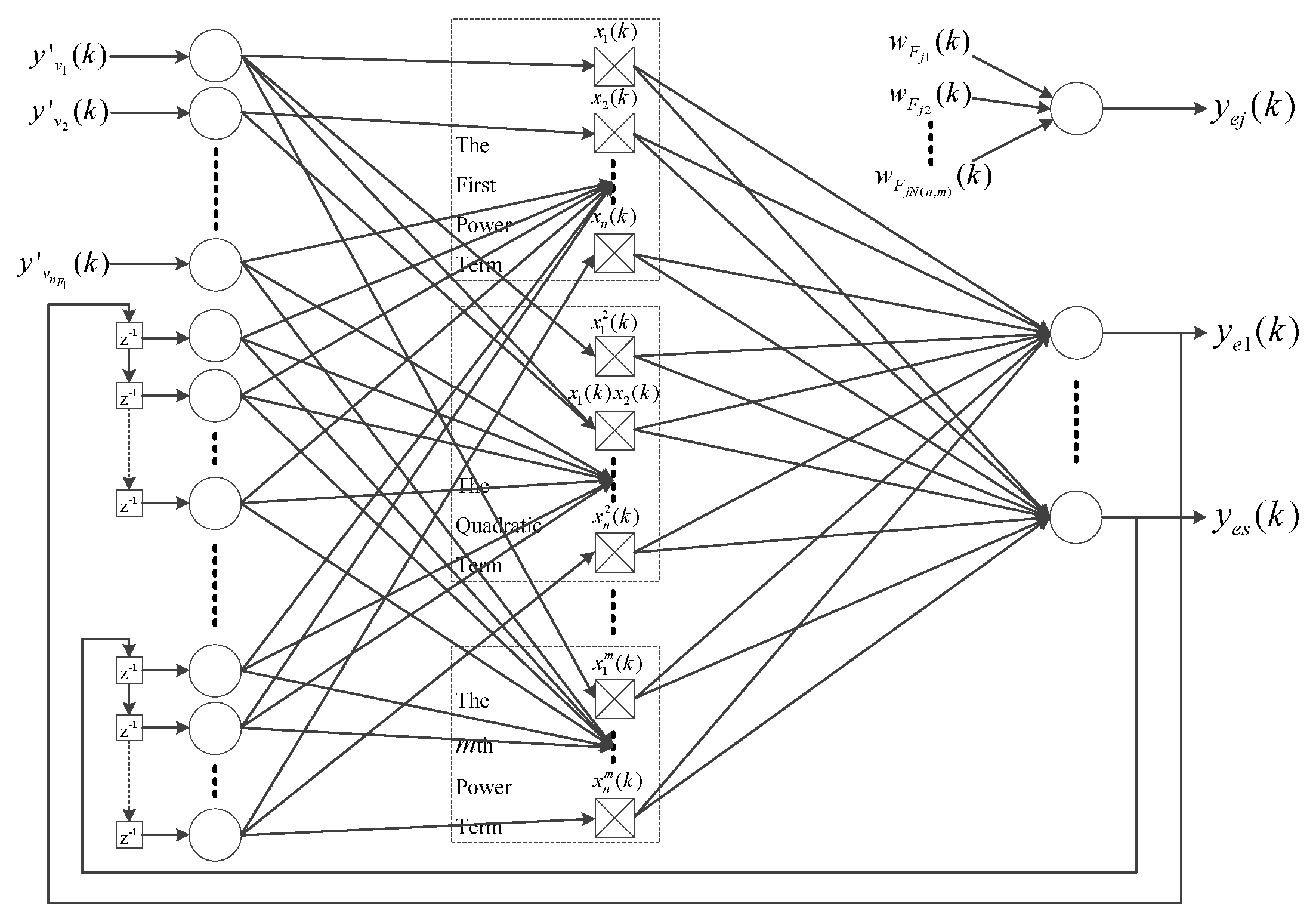
Figure 1 shows a general multi-dimensional Taylor network model with a simple structure and fast computing speed. MTN is essentially a polynomial-based nonlinear auto-regressive moving average (NARMA) model. The MTN model adopted herein is based on the polynomial-based NARMA structure, which is reused for its advantages of simple structure and linear parameterization, and is extended to the filtering scenario in this work. According to the multivariate Taylor formula, if a function has m + 1-th order derivatives in the neighborhood of a specific point, its expansion around this point is a power series of variables with order no higher than m. Consequently, for a MIMO MTN model, the universal dynamic equation suitable for an $n$-dimensional system can be expressed as

$$u_i(k)=f_{\mathrm{MTN}i}(x(k))={\displaystyle \sum _{p=1}^{N(n,m)}{w}_{ip}(k){\displaystyle \prod _{q=1}^n{x}_q^{{\lambda }_{p,q}}(k)}} {\displaystyle \sum _{p=1}^n{\lambda }_{p,q}\le m} and i=1, 2, \cdots , t$$

(3)

Note: $f_{\mathrm{MTN}i}(\cdot )$ denotes the nonlinear component within the MTN model (the underlying concept being to approximate complex functions using simple ones), which is a linear combination of polynomial product terms constructed from the system’s input/output delay signals. The summation boundary m represents the maximum order of the Taylor polynomial expansion (a predefined positive integer, e.g., m = 2 in simulations), limiting the total degree of polynomial terms to no more than m—this balances approximation accuracy and computational efficiency, consistent with MTN’s linear parameterization advantage. $w_{ip}$ stands for the $p$-th weight assigned to each term, $N(n,m)$ denotes the overall count of expansions, and ${\lambda }_{p,q}$ indicates the exponent of in the $p$-th product term.

Figure 1. Model of the multi-dimensional Taylor network.

Figure 1. Model of the multi-dimensional Taylor network.

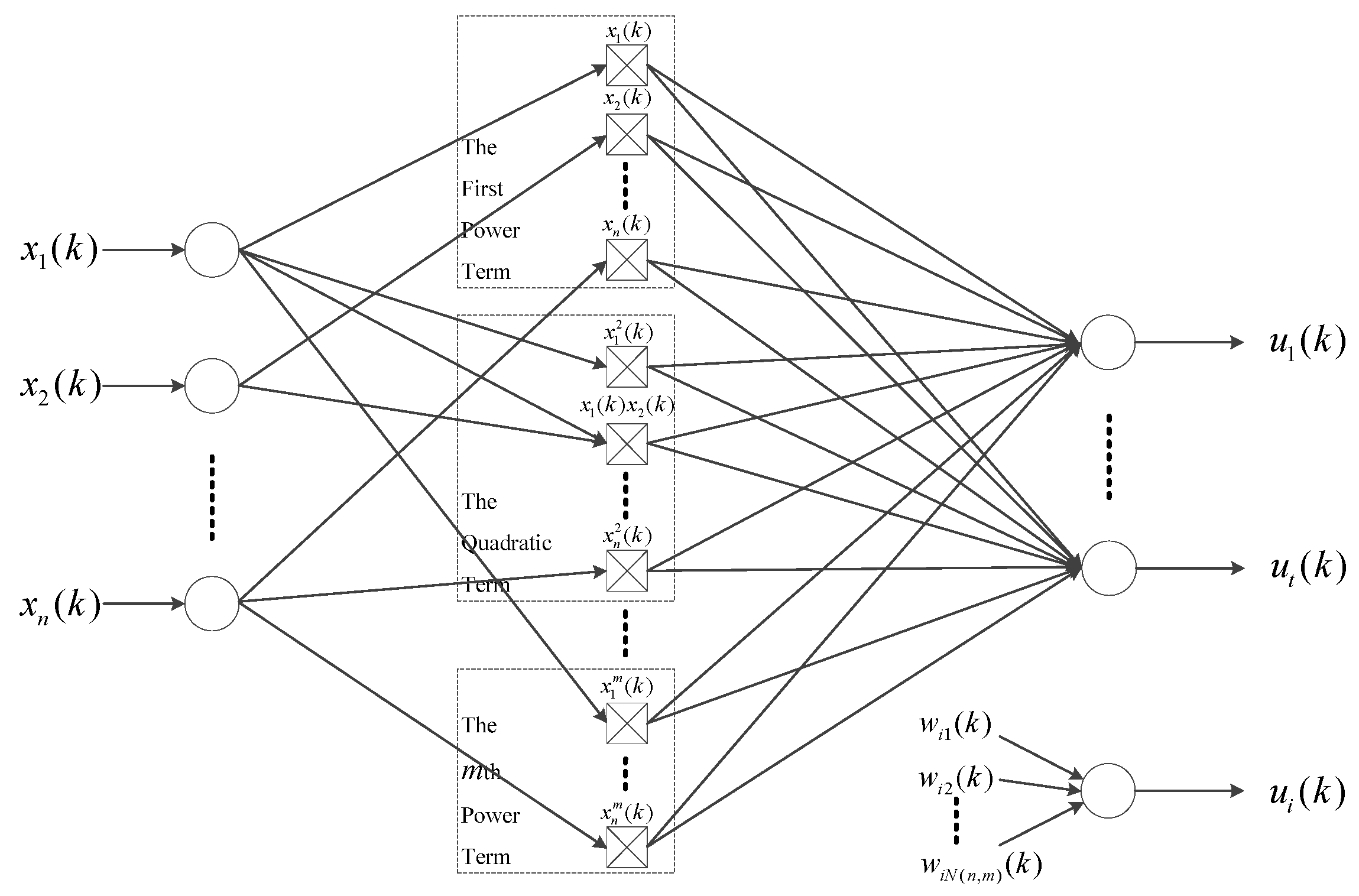
It is apparent that the MTN model employs a single intermediate layer feedforward architecture, which comprises an input layer, an intermediate layer, and an output layer. Given that $N(n,m)$ is sufficiently large, this model can achieve accurate approximations of any target model. Although (3) is a nonlinear function of the system input and output, its parameters are linearly related. Dynamic properties are incorporated via tap delay lines at the network’s input to create a dynamic MTN network controller.

The $N(n,m)$ and ${\lambda }_{p,q}$ may be derived using recursive methods, as detailed in [12].

For most industrial MIMO nonlinear systems, a maximum expansion order of m = 2 or m = 3 can achieve sufficient approximation accuracy, avoiding the explosive growth of terms caused by excessive order selection. We further adopt a contribution-based sparse term pruning mechanism, which only retains polynomial terms with a weight contribution rate higher than 1% to the final output during the adaptive update process, further reducing the number of terms and computational load in high-dimensional systems [11].

2.2.2. Approximation Capability of MTN

Lemma 1

([27]). Any continuous function defined over a closed interval can be approximated with arbitrary accuracy by a polynomial function.

Lemma 2

([11]). A continuous function $f(x_1,x_2,\cdots ,x_n)$ defined on a closed domain can be approximated by ${\displaystyle \sum _{p=1}^{N(n,m)}{w}_p}{\displaystyle \prod _{q=1}^n{x}_q^{{\lambda }_{p,q}}}$. Here, $N(n,m)$ is the total number of product terms in the expansion, $w_p$ is the weight of the p-th product term, and ${\lambda }_{p,q}$ is the exponent of variable $x_q$ in the p-th product term.

2.3. Adaptive MIMO MTN Filter

Recently, adaptive noise cancellation [25] has emerged as a prominent area of research within the field of noise elimination studies. Adaptive filters are capable of performing effectively in unknown environments and tracking temporal variations in input statistics. By continuously adjusting their weights, these systems can acclimate to the statistical characteristics of time-varying signals and noise, thereby facilitating the separation of useful signals from noise. Moreover, in scenarios where comprehensive knowledge of the noise is unavailable, adaptive filters can achieve noise cancellation by leveraging the correlation among useful signals and the lack of correlation among noise signals.

In practical industrial scenarios, the measurement noise is not limited to ideal time-independent white Gaussian noise. Correlated noises are extremely common in various industrial sensors: pink noise (1/f flicker noise) with strong low-frequency correlation is widespread in MEMS accelerometers, pressure sensors and strain gauges, while blue noise with strong high-frequency correlation is common in high-speed photoelectric sensors and high-frequency current sampling circuits. These correlated noises will cause significant steady-state bias or dynamic performance degradation in traditional filters that rely on the white noise assumption, which puts forward higher requirements for the robustness of the filtering algorithm.

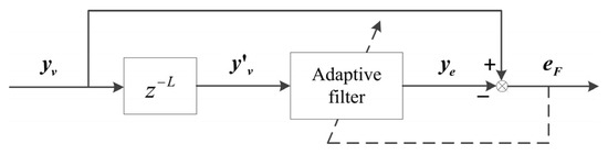
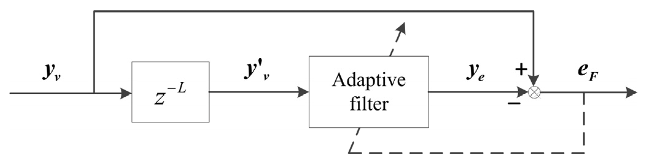
In practical applications of adaptive noise cancellation, the reference noise is difficult to identify. Therefore, the prediction principle of the adaptive filter [28] is commonly employed to eliminate the noise. Its basic principle is illustrated in Figure 2.

Figure 2. Adaptive noise cancellation with unknown reference noise (adapted from [11]).

As the white noise $v$ is time-independent, postpone signal $y_v$ mixed with noise for a certain period of time, set this delayed signal ${y^{\prime }}_v$ as the input of the adaptive MTN filter, and take the signal with noise ($y_v$) directly as the reference signal. The adaptive MTN filter can predict the signal using the strong correlation between the useful information of the delayed signal ${y^{\prime }}_v$ and the reference signal $y_v$. When noise is uncorrelated across sampling points, the filter does not estimate white noise, making its output $y_e$ the optimal approximation of the useful signal. In turn, the noise present in the filtered output $y_e$ is minimized to achieve noise elimination.

For this prediction-based noise cancellation scheme, there exists a clear upper bound of the delay parameter L, denoted as L_max, which is determined by the dynamic characteristics of the controlled system and the sampling frequency. For a practical band-limited industrial system, the coherent time of the useful signal (the longest time interval during which the signal maintains strong linear correlation) τ_c is determined by the system’s −3 dB cut-off frequency f_c, satisfying τ_c ≈ 1/f_c. With the system sampling period T_s, the theoretical upper bound of L is defined as $L_{\max }=⌊{\tau }_{\mathrm{c}}/T_{\mathrm{s}}⌋=⌊1/(f_{\mathrm{c}}\cdot T_{\mathrm{s}})⌋$, where $⌊\cdot ⌋$ denotes the floor operation. This upper bound is defined based on the engineering-recognized strong correlation threshold: the linear correlation coefficient between the delayed useful signal ${y^{\prime }}_v$ and the original useful signal $y_v$ is no less than 0.707 (the half-power point) when L ≤ L_max, which ensures the filter can extract effective features for signal prediction. When L exceeds L_max, the correlation of the useful signal is significantly lost, leading to the failure of the filter’s predictive ability. In practical design, the delay L needs to satisfy the dual constraints: (1) L ≥ 1, to ensure the white noise components in the delayed signal and the reference signal are completely uncorrelated; (2) L ≤ L_max, to retain the strong correlation of the useful signal. Thus, the reasonable value range of L is 1 ≤ L ≤ L_max.

For industrial applications, it is recommended to select L within the range of 1~L_max/3. This range can retain sufficient design margin to avoid the loss of signal correlation caused by the drift of system dynamic characteristics, and further improve the robustness of the filtering scheme in non-ideal noise scenarios.

The proposed LAF-MTNF has inherent robustness to the above-mentioned industrial correlated noises, which is derived from three core design advantages: (1) The weight update rule is completely derived based on Lyapunov stability theory, without any prior assumptions about the statistical characteristics of the noise, and will not produce steady-state bias due to the violation of the white noise assumption; (2) The strong nonlinear approximation capability of MTN can fit the complex disturbance components introduced by correlated noise, which cannot be achieved by linear adaptive filters; (3) The flexible delay L design can be adjusted according to the coherent time of the noise, ensuring sufficient de-correlation of the noise components while retaining the correlation of the useful signal.

An adaptive SISO filtering method based on Lyapunov theory [29] has been proposed and is widely used for noise reduction. Specifically, a Lyapunov function is defined to characterize the error between the filter output and the target signal; then, relying on the LST, the filter weights are adaptively adjusted to ensure the error converges asymptotically to zero. For a LAF filter, the selected Lyapunov function features a clear global minimum within the state space. Nevertheless, the findings merely outlined the fundamental concept of Lyapunov-based filtering. Numerous issues remain unaddressed, including the use of modified gain analysis to examine the convergence speed and convergence domain of adaptive filters.

In this study, we propose the use of MTN to implement LAF-IIR adaptive MIMO filters. Building on the preliminary MTN filtering idea [13], we propose an optimized LAF-MTNF with modified adaptive gain to avoid singularities, which was not resolved in the prior work. Through the proper selection of a parameter update rule in the Lyapunov framework, the output of the MTN filter can converge exponentially to the respective target signal. Given that the input signal of the adaptive MTN filter is affected by bounded random noise interference, the design of the MIMO MTN filter utilizes only input and output measurements. As a result, the design of the LAF MTN filter is not dependent on the random nature of input disturbances. Furthermore, the dynamic error index converges to zero, thereby guaranteeing system stability. It is evident that the LST offers an optimization approach for the design of MIMO MTN filters. Stated differently, this ensures both stability and convergence for the MIMO LAF MTN filter.

The advantages of this scheme mainly come from two core features: on the one hand, MTN has a unique linear structure, and its parameters can be effectively adjusted through the LAF algorithm; on the other hand, its parallel architecture provides ideal hardware support for high-speed signal processing.

The filter output $y_e(k)={[y_{e1}(k), \cdots , y_{es}(k)]}^{\mathrm{T}}$, and the desired response $y_v(k)={[y_{v1}(k), \cdots , y_{vs}(k)]}^{\mathrm{T}}$. $e_F(k)={[e_{F1}(k), \cdots , e_{Fs}(k)]}^{\mathrm{T}}$ denotes the error, which corresponds to the difference between the desired response and the filter output in Equation (4). Typically, adaptive algorithms are designed to update filter parameters in an adaptive manner, thereby minimizing the error-based cost function within the parameter space.

$$e_F(k)=y_v(k)-y_e(k)$$

(4)

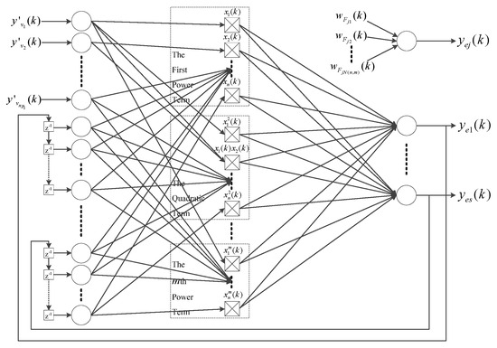
Figure 3 illustrates the construction process of the MTN-based adaptive MIMO IIR filter. The input signal ${y^{\prime }}_v(k)$ becomes distorted as a result of the controlled plant’s nonlinearity and measurement noise, that is,

$$\begin{array}{c}{{\mathit{y}}^{\prime }}_{\mathit{v}}(k)={[y{\prime }_{v_1}(k), \cdots , y{\prime }_{v_q}(k), \cdots , y{\prime }_{v_{n_{F_1}}}(k), y{\prime }_{v_{n_{F_1}+1}}(k), \cdots , y{\prime }_{v_{n_{F_1}+n_{F_2}}}(k)]}^{\mathrm{T}}\\ \hspace{1em}\hspace{1em}\hspace{1em}\hspace{1em}\hspace{1em}\hspace{1em}\hspace{1em}=[\underset{n_{F_1}}{\underbrace{y_{v1}(k-L), y_{v1}(k-L-1), \cdots , y_{v2}(k-L), y_{v2}(k-L-1), \cdots , y_{vs}(k-L), \cdots }},\\ \underset{n_{F_2}}{\underbrace{y_{e1}(k-1), y_{e1}(k-2), \cdots , y_{e2}(k-1), y_{e2}(k-2), \cdots , y_{es}(k-1), \cdots }}{]}^{\mathrm{T}}\end{array}$$

(5)

where $L$ represents the number of delays.

Figure 3. Nonlinear MIMO recurrent MTN IIR filter.

The output of the MIMO MTN IIR filter may be formulated as

$$y_e(k)=W_F(k)\phi (k)$$

(6)

where

$$W_F={[w_{F_1}(k), w_{F_2}(k), \cdots , w_{F_j}(k), \cdots , w_{F_s}(k)]}^{\mathrm{T}} j=1, 2, 3, \cdots , s,$$

$$w_{F_j}={[w_{F_{j1}}(k), w_{F_{j2}}(k), \cdots , w_{F_{jp}}(k), \cdots , w_{F_{j{N}_F}}(k)]}^{\mathrm{T}} p=1, 2, 3, \cdots , N_F,$$

$$\phi (k)={[{\phi }_1(k), {\phi }_2(k), \cdots , {\phi }_p(k), \cdots , {\phi }_{N_F}(k)]}^{\mathrm{T}},$$

$\phi (k)$ is defined as a function of the Taylor type, expressed as ${\varphi }_p(k)={\displaystyle \prod _{q=1}^{n_{F_1}+n_{F_2}}y{\prime }_{v_q}^{{\lambda }_{p,q}}(k)}$ and $\lambda (p,q)$ in [12].

In the course of analyzing the input–output relationship within the measurement process, we find that

$$y_v=W_F\phi +v$$

(7)

where $W_{F_{s\times N_F}}$ denotes the system parameter matrix of the MTN that awaits estimation, $\phi ={[{\phi }_1, \cdots , {\phi }_{N_F}]}^{\mathrm{T}}$ stands for the measured vector, and $v={[v_1, \cdots , v_s]}^{\mathrm{T}}$ is the unknown measurement noise of the system.

At time step $k$, the filtering error, which arises from the discrepancy between the measured value and the output of the adaptive MIMO MTN filter, is defined as

$$e_F(k)=y_v(k)-W_F(k)\phi (k)$$

(8)

And the prediction error is

$$e_P(k)=y_v(k)-W_F(k-1)\phi (k)$$

(9)

Based on this, using Equation (7) as the measurement equation, an adaptive LAF algorithm for the MIMO system can be constructed, and the process is as follows:

$$W_F(k)=W_F(k-1)+e_P(k)K(k)$$

(10)

$$K(k)={\displaystyle \frac{{\phi }^{\mathrm{T}}(k)}{{‖\phi (k)‖}^2}}\left[1-e^{-\gamma }{\displaystyle \frac{‖e_F(k-1)‖}{‖e_P(k)‖}}\right]$$

(11)

To avoid singularities in the gain $K(k)$ within Equation (11) when $‖\phi (k)‖$ and $‖e_P(k)‖$ approach zero, Equation (11) is revised to form Equation (12):

$$K(k)={\displaystyle \frac{{\phi }^{\mathrm{T}}(k)}{{\kappa }_1+{‖\phi (k)‖}^2}}\left[1-e^{-\gamma }{\displaystyle \frac{‖e_F(k-1)‖}{{\kappa }_2+‖e_P(k)‖}}\right]$$

(12)

where $K(k)$ denotes the adaptive gain, $‖\cdot ‖$ represents the Euclidean norm of the vector, ${\kappa }_1$ and ${\kappa }_2$ are small positive constants introduced to avoid singularities, and $e^{-\gamma }$ corresponds to the natural exponential function, with $\gamma$ being a positive constant that regulates the convergence speed of the LAF algorithm. The larger $\gamma$ is, the faster the error converges.

The two constants (${\kappa }_1$ and ${\kappa }_2$) work together to ensure the denominator remains strictly positive when the measured vector $‖\phi (k)‖$ and filtering error $‖e_P(k)‖$ approach zero simultaneously, completely eliminating the singularity risk of the adaptive gain tending to infinity. Among them, ${\kappa }_2$ is the dominant offset term, which directly determines the core performance trade-off:

(1)

When ${\kappa }_2$ is too small (e.g., ${\kappa }_2$ < 10⁻⁵), the singularity avoidance effect is significantly weakened, which may cause instantaneous spikes in the adaptive gain, numerical oscillation of weight update, and even algorithm divergence;

(2)

When ${\kappa }_2$ is too large (e.g., ${\kappa }_2$ > 10⁻¹), the adaptive gain will be excessively compressed, leading to stagnant weight update and significant steady-state bias;

(3)

The optimal value range of ${\kappa }_2$ is 10⁻⁴ ≤ ${\kappa }_2$ ≤ 10⁻², which achieves the best balance of stability, accuracy and convergence speed. The auxiliary constant ${\kappa }_1$ is set to match the order of ${\kappa }_2$ to further enhance the robustness of singularity avoidance, without affecting the core performance trade-off.

For practical industrial applications, it is recommended to set ${\kappa }_2$ to 1/10 ~ 1/100 of the standard deviation of the system measurement noise, and set ${\kappa }_1$ to the same order of magnitude as ${\kappa }_2$, to quickly match the actual working conditions and ensure the robustness of the algorithm.

γ is a positive constant satisfying γ ≥ 1, which dominates the convergence speed of the algorithm: the larger the γ value, the larger the weight update step, and the faster the convergence speed. The practical upper bound of γ derived from the Lyapunov stability criterion is ${\gamma }_{\max }={\displaystyle \frac{2}{T_s\cdot {‖{y^{\prime }}_v(k)‖}_{\max }^2}}$, where T_s is the system sampling period, and ${‖{y^{\prime }}_v(k)‖}_{\max }$ is the maximum amplitude of the system input signal. When γ exceeds γ_max, the oversized update step will break the monotonic non-increasing property of the Lyapunov function, resulting in numerical oscillation or even system divergence. For practical applications, it is recommended to set γ within 1 ≤ γ ≤ γ_max/2 to balance fast convergence and sufficient stability margin.

2.4. Stability and Convergence of MIMO LAF Algorithm

Compared with the basic stability analysis [13], Theorem 1 in this work further quantifies the error convergence rate and region, ensuring asymptotic stability of the filtering system.

Theorem 1.

The adaptive MIMO LAF MTN filtering algorithm maintains stability when  $e^{-\gamma }$  satisfies inequality (13). Additionally, because the weights of the MTN IIR filter undergo adaptive updates via the modified laws (10) and (12), the error will converge exponentially toward a sphere within the error space—this sphere is centered at the origin, and its radius is defined by Equation (14).

$$e^{-\gamma }<{\displaystyle \frac{4}{3{\kappa }_2}}$$

(13)

$$\rho ={\displaystyle \frac{6{\kappa }_2{e}^{-\gamma }-8{\kappa }_2}{9e^{-2\gamma }-16}}$$

(14)

Proof. 

This proof is derived based on Assumption 1. To analyze the stability of the algorithm, we first define a Lyapunov function for the filtering error as shown in Equation (15).

$$V_F(k)={‖e_F(k)‖}^2$$

(15)

Substituting the filtering error definition (Equation (8)) into Equation (15), we derive

$$\begin{array}{cc}\hfill \mathrm{\Delta }{V}_F(k)& =V_F(k)-V_F(k-1)={‖e_F(k)‖}^2-{‖e_F(k-1)‖}^2={‖y_v(k)-W_F(k)\phi (k)‖}^2-{‖e_F(k-1)‖}^2\hfill \\ & ={‖y_v(k)-W_F(k-1)\phi (k)-e_P(k)K(k)\phi (k)‖}^2-{‖e_F(k-1)‖}^2={‖e_P(k)-e_P(k)K(k)\phi (k)‖}^2-{‖e_F(k-1)‖}^2\hfill \\ & ={‖e_P(k)‖}^2{\left|1-{\displaystyle \frac{{\phi }^{\mathrm{T}}(k)}{{\kappa }_1+{‖\phi (k)‖}^2}}\left[1-e^{-\gamma }{\displaystyle \frac{‖e_F(k-1)‖}{{\kappa }_2+‖e_P(k)‖}}\right]\phi (k)\right|}^2-{‖e_F(k-1)‖}^2\hfill \\ & ={‖e_P(k)‖}^2{\left|1-{\displaystyle \frac{\frac{{‖\phi (k)‖}^2}{{\kappa }_1}}{1+\frac{{‖\phi (k)‖}^2}{{\kappa }_1}}}\left[1-{\displaystyle \frac{e^{-\gamma }}{{\kappa }_2}}{\displaystyle \frac{‖e_F(k-1)‖}{1+\frac{‖e_P(k)‖}{{\kappa }_2}}}\right]\right|}^2-{‖e_F(k-1)‖}^2\hfill \end{array}$$

(16)

where $\left({‖\phi (k)‖}^2/{\kappa }_1\right)<1$ and $\left(‖e_P(k)‖/{\kappa }_2\right)<1$. The singularity-avoidance constants ${\kappa }_1$ and ${\kappa }_2$ in Equation (12) are included in the derivation of the convergence region radius in Equation (14). Within the recommended optimal value range, their impact on the convergence region is negligible and will not affect the asymptotic convergence of the filtering error.

The two norms compared with 1 herein satisfy $‖\cdot ‖<1$. This premise is justified by the convergence characteristic of adaptive filtering: as the algorithm iterates, the filtering error converges to a small neighborhood around zero, making the norms of error-related vectors sufficiently small. Comparing with 1 enables us to neglect higher-order remainder terms in the subsequent Taylor expansion (Equations (17) and (18))—since $‖\cdot ‖<1$ implies higher-order powers (e.g., ${‖\cdot ‖}^2$) are negligible infinitesimals—thus simplifying the nonlinear Lyapunov function derivative into a tractable parabolic function for stability analysis.

Apply the Taylor series expansion to the following equation:

$${\displaystyle \frac{\frac{{‖\phi (k)‖}^2}{{\kappa }_1}}{1+\frac{{‖\phi (k)‖}^2}{{\kappa }_1}}}={\displaystyle \frac{{‖\phi (k)‖}^2}{{\kappa }_1}}+\mathrm{O}\left({\displaystyle \frac{{‖\phi (k)‖}^2}{{\kappa }_1}}\right)$$

(17)

$${\displaystyle \frac{1}{1+\frac{‖e_P(k)‖}{{\kappa }_2}}}=1-{\displaystyle \frac{‖e_P(k)‖}{{\kappa }_2}}+\mathrm{O}\left({\displaystyle \frac{‖e_P(k)‖}{{\kappa }_2}}\right)$$

(18)

where

$$\left|\mathrm{O}\left({\displaystyle \frac{{‖\phi (k)‖}^2}{{\kappa }_1}}\right)\right|=\left|{\displaystyle \frac{{‖\phi (k)‖}^2}{{‖\phi (k)‖}^2+{\kappa }_1}}-{\displaystyle \frac{{‖\phi (k)‖}^2}{{\kappa }_1}}\right|\le \left|{\displaystyle \frac{1}{2}}-1\right|={\displaystyle \frac{1}{2}}$$

$$\left|\mathrm{O}\left({\displaystyle \frac{‖e_P(k)‖}{{\kappa }_2}}\right)\right|=\left|{\displaystyle \frac{{\kappa }_2}{{\kappa }_2+‖e_P(k)‖}}-1+{\displaystyle \frac{‖e_P(k)‖}{{\kappa }_2}}\right|\le \left|{\displaystyle \frac{1}{2}}-1+1\right|={\displaystyle \frac{1}{2}}$$

Then, (16) can be rewritten as

$$\mathrm{\Delta }{V}_F(k)={‖e_P(k)‖}^2 {\left|1-\left({\displaystyle \frac{{‖\phi (k)‖}^2}{{\kappa }_1}}+\mathrm{O}\left({\displaystyle \frac{{‖\phi (k)‖}^2}{{\kappa }_1}}\right)\right) \left[1-{\displaystyle \frac{e^{-\gamma }‖e_F(k-1)‖}{{\kappa }_2}}\left(1-{\displaystyle \frac{‖e_P(k)‖}{{\kappa }_2}}+\mathrm{O}\left({\displaystyle \frac{‖e_P(k)‖}{{\kappa }_2}}\right)\right)\right]\right|}^2 -{‖e_F(k-1)‖}^2$$

(19)

Thus, we obtain

$$\begin{array}{cc}\hfill \mathrm{\Delta }{V}_F(k)& \le {\kappa }_2^2{\left|1-\left(1+{\displaystyle \frac{1}{2}}\right)\left(1-{\displaystyle \frac{e^{-\gamma }‖e_F(k-1)‖}{{\kappa }_2}}\left(1-1+{\displaystyle \frac{1}{2}}\right)\right)\right|}^2-{‖e_F(k-1)‖}^2\hfill \\ & \le {\kappa }_2^2{\left|1-{\displaystyle \frac{3}{2}}+{\displaystyle \frac{3e^{-\gamma }‖e_F(k-1)‖}{4{\kappa }_2}}\right|}^2-{‖e_F(k-1)‖}^2\hfill \\ & ={\kappa }_2^2{\left|{\displaystyle \frac{3e^{-\gamma }‖e_F(k-1)‖}{4{\kappa }_2}}-{\displaystyle \frac{1}{2}}\right|}^2-{‖e_F(k-1)‖}^2\hfill \\ & ={\kappa }_2^2\left|{\displaystyle \frac{9e^{-2\gamma }{‖e_F(k-1)‖}^2}{16{\kappa }_2^2}}-{\displaystyle \frac{3e^{-\gamma }‖e_F(k-1)‖}{4{\kappa }_2}}+{\displaystyle \frac{1}{4}}\right|-{‖e_F(k-1)‖}^2\hfill \end{array}$$

(20)

Now, we have to start splitting in the following situations.

• If ${\displaystyle \frac{‖e_F(k-1)‖e^{-\gamma }}{{\kappa }_2}}\ge {\displaystyle \frac{2}{3}}$, i.e., $e^{-\gamma }\ge {\displaystyle \frac{2{\kappa }_2}{3‖e_F(k-1)‖}}$,

Equation (20) can be rewritten as

$$\mathrm{\Delta }{V}_F(k)\le \left({\displaystyle \frac{9}{16}}{e}^{-2\gamma }-1\right){‖e_F(k-1)‖}^2-{\displaystyle \frac{3}{4}}{\kappa }_2{e}^{-\gamma }‖e_F(k-1)‖+{\displaystyle \frac{1}{4}}{\kappa }_2^2$$

(21)

Then, the following parabolic function is considered:

$$\mathrm{\Delta }{\tilde{V}}_F(k)=\left({\displaystyle \frac{9}{16}}{e}^{-2\gamma }-1\right){‖e_F(k-1)‖}^2-{\displaystyle \frac{3}{4}}{\kappa }_2{e}^{-\gamma }‖e_F(k-1)‖+{\displaystyle \frac{1}{4}}{\kappa }_2^2$$

(22)

If $\gamma$ is big enough ($e^{-\gamma }$ is small enough), in the sense that $\left(9e^{-2\gamma }/16\right)<1$ or $\left(3{\kappa }_2{e}^{-\gamma }/4\right)<1$, then we have $e^{-\gamma }<\left(4/3{\kappa }_2\right)$, and $\mathrm{\Delta }{\tilde{V}}_F(k)$ becomes a downward concave parabolic function. Moreover, with the values ${\kappa }_1$ and ${\kappa }_2$ given, the small positive parameter $e^{-\gamma }$ satisfies the inequality below:

$$e^{-\gamma }<{\displaystyle \frac{4}{3{\kappa }_2}}\mathrm{or} \gamma >-\ln \left({\displaystyle \frac{4}{3{\kappa }_2}}\right)$$

(23)

To find the values that make b = 0, we solve the quadratic Equation (22), which yields two roots, i.e.,

$$\begin{array}{cc}{\rho }_{1,2}& ={\displaystyle \frac{\frac{3}{4}{\kappa }_2{e}^{-\gamma }\pm \sqrt{{\left(\frac{3}{4}{\kappa }_2{e}^{-\gamma }\right)}^2-4\left(\frac{9}{16}{e}^{-2\gamma }-1\right)\left(\frac{1}{4}{\kappa }_2^2\right)}}{2\left(\frac{9}{16}{e}^{-2\gamma }-1\right)}}\hfill \\ & ={\displaystyle \frac{\frac{3}{4}{\kappa }_2{e}^{-\gamma }\pm \sqrt{\frac{9}{16}{\kappa }_2^2{e}^{-2\gamma }-\frac{9}{16}{\kappa }_2^2{e}^{-2\gamma }+{\kappa }_2^2}}{\frac{9}{8}{e}^{-2\gamma }-2}}={\displaystyle \frac{6{\kappa }_2{e}^{-\gamma }\pm 8{\kappa }_2}{9e^{-2\gamma }-16}}\hfill \end{array}$$

(24)

The root ${\rho }_2$ is derived from $‖e_F(k-1)‖\ge 0$, i.e.,

$${\rho }_2={\displaystyle \frac{6{\kappa }_2{e}^{-\gamma }-8{\kappa }_2}{9e^{-2\gamma }-16}}$$

(25)

Hence, $‖e_F(k-1)‖$ must satisfy inequality (26), as follows:

$$‖e_F(k-1)‖>{\rho }_2$$

(26)

Then, we have $\mathrm{\Delta }{V}_F(k)<\mathrm{\Delta }{\tilde{V}}_F(k)<0$. Afterwards, the error will converge toward a ball within the error space. This ball is centered at the origin, and its radius ${\rho }_2$ is defined by Equation (25).

2.

If ${\displaystyle \frac{‖e_F(k-1)‖e^{-\gamma }}{{\kappa }_2}}<{\displaystyle \frac{2}{3}}$, i.e., $e^{-\gamma }<{\displaystyle \frac{2{\kappa }_2}{3‖e_F(k-1)‖}}$,

Equation (20) can be re-expressed as

$$\mathrm{\Delta }{V}_F(k)\le \left(-{\displaystyle \frac{9}{16}}{e}^{-2\gamma }-1\right){‖e_F(k-1)‖}^2+{\displaystyle \frac{3}{4}}{\kappa }_2{e}^{-\gamma }‖e_F(k-1)‖-{\displaystyle \frac{1}{4}}{\kappa }_2^2$$

(27)

Then, the following parabolic function is considered:

$$\mathrm{\Delta }{\tilde{V}}_F(k)=\left(-{\displaystyle \frac{9}{16}}{e}^{-2\gamma }-1\right){‖e_F(k-1)‖}^2+{\displaystyle \frac{3}{4}}{\kappa }_2{e}^{-\gamma }‖e_F(k-1)‖-{\displaystyle \frac{1}{4}}{\kappa }_2^2$$

(28)

As $e^{-\gamma }>0$, i.e., $\left(-\left(9e^{-2\gamma }/16\right)-1\right)<0$, so $\mathrm{\Delta }{\tilde{V}}_F(k)$ takes the form of a downward concave parabolic function. Moreover, given values for ${\kappa }_1$ and ${\kappa }_2$,

$$\mathrm{\Delta }={\left({\displaystyle \frac{3}{4}}{\kappa }_2{e}^{-\gamma }\right)}^2-4\left(-{\displaystyle \frac{9}{16}}{e}^{-2\gamma }-1\right)\left(-{\displaystyle \frac{1}{4}}{\kappa }_2^2\right)=-{\kappa }_2^2<0$$

(29)

Hence, there exists no solution in this situation ($e^{-\gamma }<\left(2{\kappa }_2/3‖e_F(k-1)‖\right)$). □

That completes the whole proof. It should be clarified that the convergence radius defined in this theorem is completely independent of the magnitude of exogenous measurement noise, and is solely determined by the system’s structural parameters and filter design parameters. The magnitude of measurement noise only affects the final bounded domain (steady-state error “sphere”) of the filtering error: larger noise will lead to a larger steady-state error bound. The convergence radius in this theorem is always far larger than the maximum steady-state error bound under conventional industrial measurement noise conditions, ensuring the global convergence of the algorithm.

Theorem 1 confirms that the stability of the adaptive MIMO LAF MTN filtering system can be validated on the basis of Lyapunov stability theory. As the number of iterations increases, the convergence of the system is accelerated, and the filtering error converges to zero.

3. Adaptive MIMO MTN Control

3.1. Control System Structure

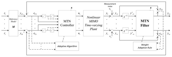
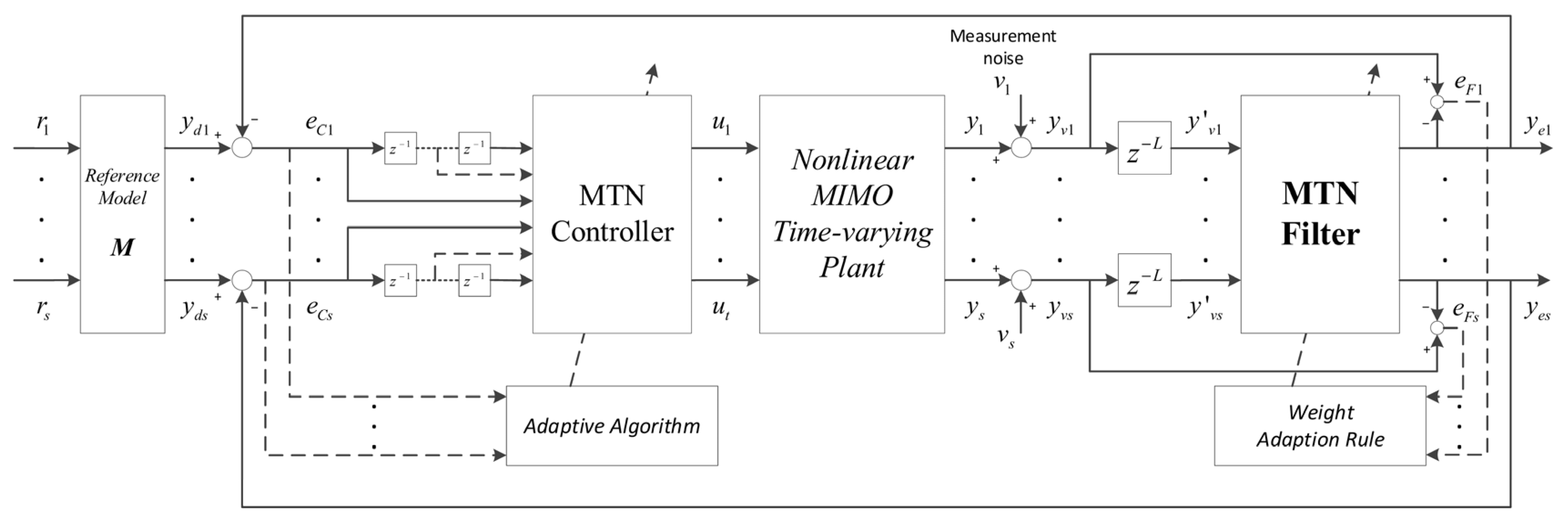
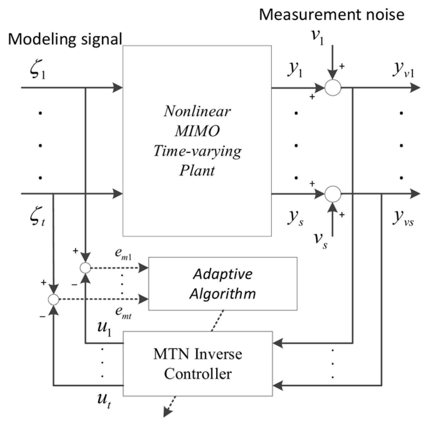
The control system employs a closed-loop control configuration, consisting primarily of three components: a controller, a controlled system, and a filter. Both the controller and the filter are constructed using an adaptive multi-dimensional Taylor network, as depicted in Figure 4. This approach is applicable to electrical and mechanical systems characterized by reversible, unknown, and nonlinear functions.

Figure 4. Structure of MTN control system (adapted from [13]).

Within the entire control system, $y_d$ denotes the object vector, $e_C$ represents the error vector, $u$ stands for the control law, $y$ is the output value, $y_v$ refers to the output signal contaminated by noise, and $y_e$ signifies the filtered output signal. The control algorithm is outlined in Algorithm 1.

Algorithm 1. Controlling algorithm for complex nonlinear systems, e.g., MIMO nonlinear systems characterized by time variation, uncertainty, and measurement noises.

1: Initialize the weights of MTNC by inverse modeling. This method is detailed in [12] and will not be repeated here for brevity; 2: The controller receives the input of the controlled system’s object values; 3: Use MTNC to control the controlled system; 4: The system output containing noise is read by a measurement sensor; 5: MTNF serves to eliminate random disturbances, such as control disturbances and measurement noise, while an enhanced LAF algorithm is used to update its weights. The proposed method is detailed in Section 2.3 and will not be repeated here for brevity; 6: Feedback on the filtered output of the control system; 7: A modified gradient descent method is used in [13] to tune the parameters of MTNC; 8: Should the control error be sufficiently small, the algorithm should be terminated. Otherwise, revert to step 3.

It should be clarified that the inverse modeling initialization in Algorithm 1 is designed for the closed-loop controller weights, not the filter weights. This strategy aims to improve the controller’s initial adaptability to the time-varying characteristics and uncertainties of the controlled plant and accelerate the initial dynamic response of the closed-loop system. The filter introduced to suppress complex measurement noise only needs simple random initialization. Its global stability is guaranteed by the Lyapunov criterion, which is completely insensitive to poor initialization. Even with random initial weights, the filter maintains stable asymptotic convergence, showing strong robustness to initial value selection.

3.2. Design of Initial MIMO MTN Controller

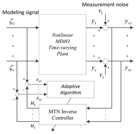
To secure the stability of adaptive control systems during their initial phase, developing an offline MTN controller (via offline MIMO inverse modeling) represents a primary and indispensable step in creating online adaptive MTN controllers. Offline trials require a large collection of training samples to ensure that adaptive MIMO feedback controllers can cover the entire operational spectrum. Generally, white noise functions as the modeling signal to support the offline MIMO inverse modeling procedure.

As illustrated in Figure 5, the offline MTN controller is constructed using the direct approach [30], which involves directly modeling the MIMO inverse of a target through its input and output data. More precisely, this technique uses the target’s output as the input for the MTN, aiming to make the MTN’s output closely resemble the target’s input. While straightforward, this method lacks training in the target’s direction, restricting it to offline implementation.

Figure 5. Structure for offline MIMO inverse modeling.

4. Analysis of Computational Complexity

Computational complexity is important for nonlinear adaptive controllers. But it is unrealistic to compare computation times across computers. Furthermore, it is necessary to estimate the computational complexity without relying on a computer.

Golub [31] highlights that the number of floating-point operations (FLOPs) can serve as an indicator for evaluating computational load. For example, both addition and multiplication are considered single FLOPs. The total number of these operations, which reflects the computational workload of a controller, can be evaluated by comparing the number of operations involved in each step of the computation. The computational complexity of the MTN controller is evaluated as follows. A significant advantage of MTN is that it only requires simple arithmetic operations to meet real-time control requirements and has a very lightweight architecture. In contrast, neural networks (NNs) often face high computational loads due to exponential operations, and their real-time processing capabilities are also limited [32].

In Table 1, we strictly follow the classical FLOPs statistical norms for real-time control systems [31]: 1 single-precision floating-point addition and 1 multiplication are each counted as 1 FLOP; 1 exponential operation (exp()) is equivalent to 20 basic FLOPs, which reflects the actual hardware overhead of nonlinear activation functions. The total FLOPs per iteration cover all operations required for the filter’s forward output calculation and real-time adaptive weight update. To ensure a fair comparison, both methods adopt a structure fully aligned with the simulation experiment: 6 input nodes, 2 output nodes, with 27 intermediate nodes for MTN (2nd-order Taylor expansion) and 27 hidden layer nodes for the RBFNN benchmark.

Table 1. FLOPs per iteration comparison between MTN and RBFNN.

Metric	MTN Controller	MTN Filter	RBFNN Controller and Filter
Addition Operations per Iteration	52	52	456
Multiplication Operations per Iteration	96	96	840
Exponential Operations per Iteration (Equivalent FLOPs)	0	0	1080
Total FLOPs per Iteration	296		2376

Notes: Exponential operations include the calculations required for the Gaussian activation function in forward propagation and partial derivative calculation in adaptive weight update.

In the given example where ($t=z=2$), the MTN optimal controller requires only 296 FLOPs, while that of the RBFNN controller requires 1296—the MTN’s computational load is only ~23% of RBFNN, which directly translates to superior real-time performance. The comparison results quantitatively verify that the total FLOPs per iteration of the MTN is only 6.2% of the benchmark RBFNN. More importantly, the proposed method completely avoids the exponential computational load of RBFNN from two core dimensions: (1) it has no high-overhead exponential activation function operations; (2) its computational load grows in a controllable polynomial manner with the system dimension, rather than the exponential growth of RBFNN when scaling to high-dimensional MIMO systems. This significant computational advantage is derived from the inherent linear parameterization characteristic of MTN. This indicates that MTN’s low computational complexity is not just a theoretical advantage, but a critical guarantee for meeting the real-time requirements of highly dynamic industrial scenarios (e.g., permanent magnet synchronous motor speed control, robot joint trajectory tracking).

For high-dimensional MIMO systems with more than 3 inputs/outputs, the proposed LAF-MTNF still maintains a significant computational efficiency advantage. The detailed FLOPs comparison results under different system dimensions are summarized in Table 2.

Table 2. Computational complexity comparison of different filtering algorithms in high-dimensional MIMO systems.

System Dimension (Input/Output)	Maximum Expansion Order/Hidden Layer Nodes	Total Single-Step Flops of Proposed LAF-MTNF	Total Single-Step Flops of RBFNN-LAF Benchmark	Flops Ratio (MTN/RBFNN)
3-input/3-output	m = 2/6 hidden nodes	1.28 × 103	4.74 × 103	27.0%
4-input/4-output	m = 2/8 hidden nodes	2.15 × 103	6.94 × 103	31.0%

Notes: All tests are conducted under consistent parameter settings to ensure fair comparison of approximation capability: the maximum expansion order of MTN is m = 2, and the number of hidden layer nodes of the RBFNN benchmark is set to 2× the number of input variables.

The above results verify that the polynomial growth of MTN terms has obvious scalability advantages over the rapid growth of RBFNN computational complexity in high-dimensional scenarios, and the proposed method can still maintain excellent computational efficiency in MIMO systems with more than 3 inputs/outputs.

5. Simulation

The simulation is carried out based on the widely recognized MIMO nonlinear servo system benchmark model proposed in [21], which has been extensively adopted by the academic community for the validation of MIMO adaptive control and filtering algorithms in industrial scenarios, as determined by (30). This benchmark model fully covers the core characteristics of practical industrial systems, including strong inter-channel coupling, fast time-varying dynamics, unknown nonlinearity and complex measurement disturbances, and is fully compatible with the dynamic characteristics of power electronic systems, industrial servo motion systems and process control systems.

$$\left\{\begin{array}{l}{y}_1(k)={\displaystyle \frac{f_{11}(k)y_1(k-1)+f_{12}(k)}{1+y_1^2(k-1)}}+f_{13}(k)y_2(k-2)+f_{14}(k)u_1(k-1)+f_{15}(k)u_2(k-2)+v_1(k-1)\\ y_2(k)=f_{21}(k)y_1(k-2)+{\displaystyle \frac{f_{22}(k)y_2(k-1)+f_{23}(k)}{1+y_2^2(k-1)}}+f_{24}(k)u_1(k-2)+f_{25}(k)u_2(k-1)+v_2(k-1)\end{array}\right.$$

(30)

where $u_1$ and $u_2$ are the control laws, $f_{11}(k)=1.06\left(1-e^{-0.6(k-1)}\right)$, $f_{12}(k)=0.52\lg k$, $f_{13}(k)=e^{-0.6(k-1)}$, $f_{14}(k)=0.8$, $f_{15}(k)=e^{-0.6(k-1)}$, $f_{21}(k)=e^{-0.8(k-1)}$, $f_{22}(k)=1.06\left(1-e^{-0.8(k-1)}\right)$, $f_{23}(k)=0.28\lg k$, $f_{24}(k)=e^{-0.8(k-1)}$, $f_{25}(k)=0.6$, and $v(k)$ represents white Gaussian noise characterized by a mean of 0 and a standard deviation of 0.05.

All types of noise used in the simulation experiments strictly comply with Assumption 1 (Boundedness of Measurement Noise), with a clear amplitude upper bound set for each noise scenario, which is fully consistent with the theoretical premise of the algorithm. The singularity-avoidance constants are set to ${\kappa }_1$ = 10⁻³ and ${\kappa }_2$ = 10⁻³, which are within the recommended optimal range and match the standard deviation of the measurement noise (0.05) in the simulation, ensuring the optimal balance of filtering stability and accuracy. γ is set to 8, which is within the recommended stable range (about 1/3 of the calculated γ_max = 24), fully satisfying γ ≥ 1, ensuring both fast convergence speed and reliable numerical stability.

In this simulation, the sampling period T_s is set to 0.01 s (sampling frequency f_s = 100 Hz), and the −3 dB cut-off frequency of the controlled MIMO nonlinear system is about 10 Hz. According to the upper bound definition, we can calculate that τ_c ≈ 0.1 s and L_max = 10. The delay L is set to 1 in this simulation, which is completely within the reasonable range of 1 ≤ L ≤ L_max, ensuring the strong correlation of the useful signal and the uncorrelation of the noise.

To illustrate the merits of the MTN controller and filter, the results from the simulation experiment of (30) are compared between MTN and RBFNN. The following parameters are set for the system.

After initializing the MTNC weights via inverse modeling [12], we set the number of iterations to 50 and the sampling interval to 0.01 s. The MTNC adopts a 6-27-2 structure, with 6 input nodes, 2 expansion orders, and an initial learning rate of 0.1. Consistent with the above, the MTNF network size is set to 6-27-2, that is, 6 input layer nodes, and the second-order functional extension is completed.

Under the designed adaptive RBFNN control architecture, the RBFNN controller (RBFNNC) consists of a three-layer network: the first layer is configured with 6 input units, the middle layer contains 27 nodes, and the output layer has 2 neurons. The initial values of the weight parameters are randomly chosen within the range (−1, 1), and the RBFNNC undergoes training via the linear reinforcement method with an adaptive variable step size. During the training phase, the learning factor is set to 0.1. An RBFNN filter (RBFNNF) is constructed using a three-layer NN that shares the same 6-27-2 structure. Initial values of the weight parameters are also selected in a random way in the interval (−1,1), and the LAF algorithm is employed to train RBFNNF in the training process.

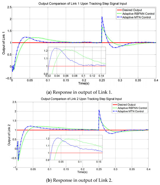
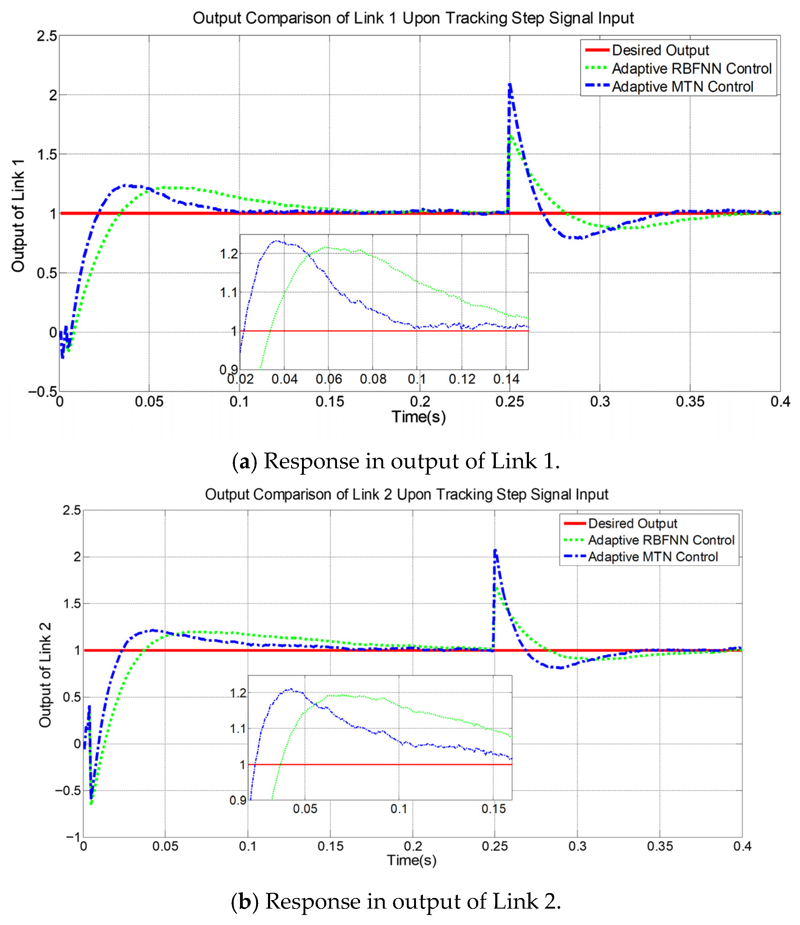
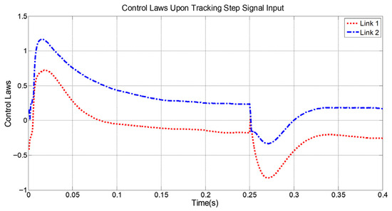
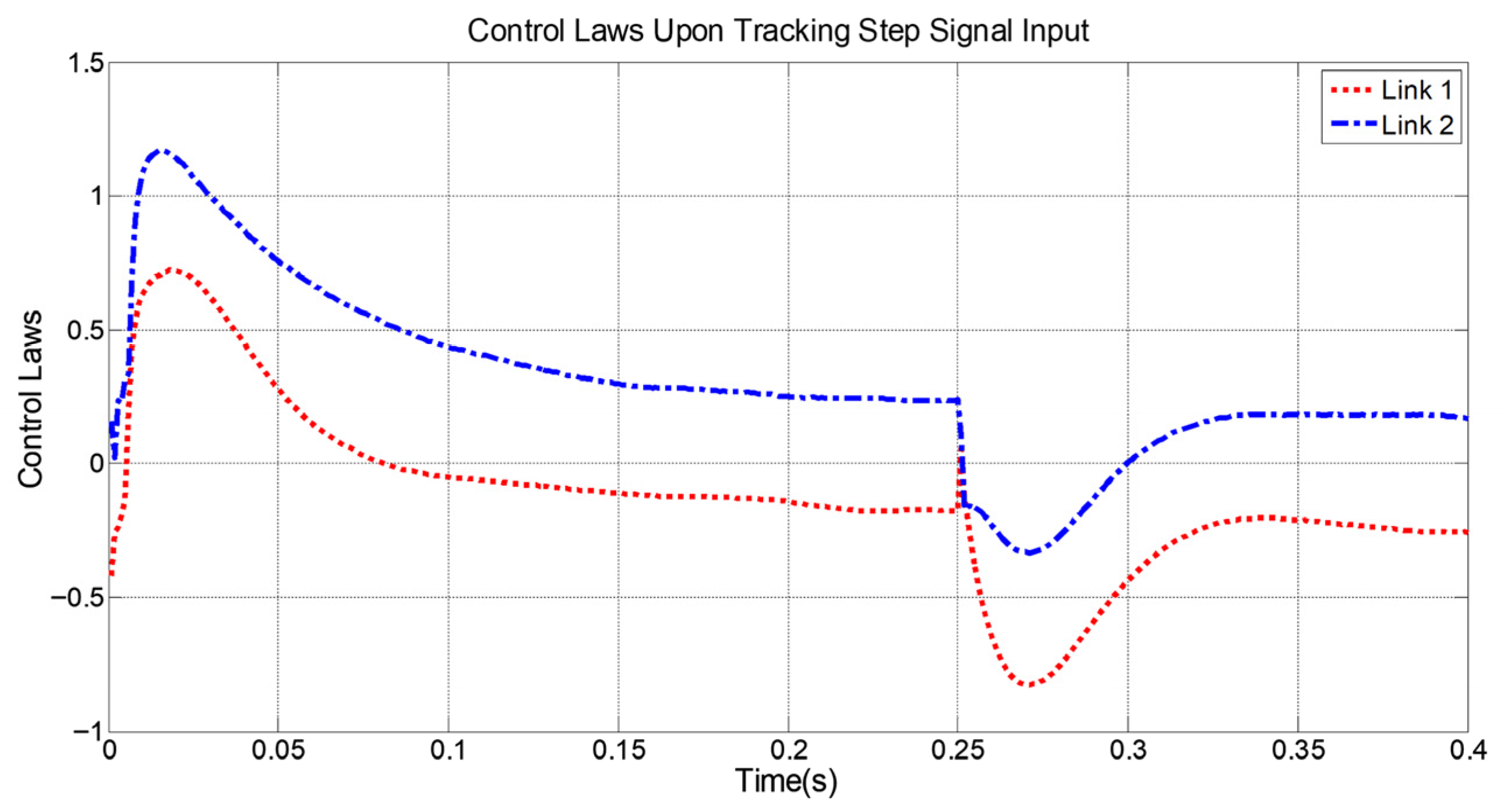
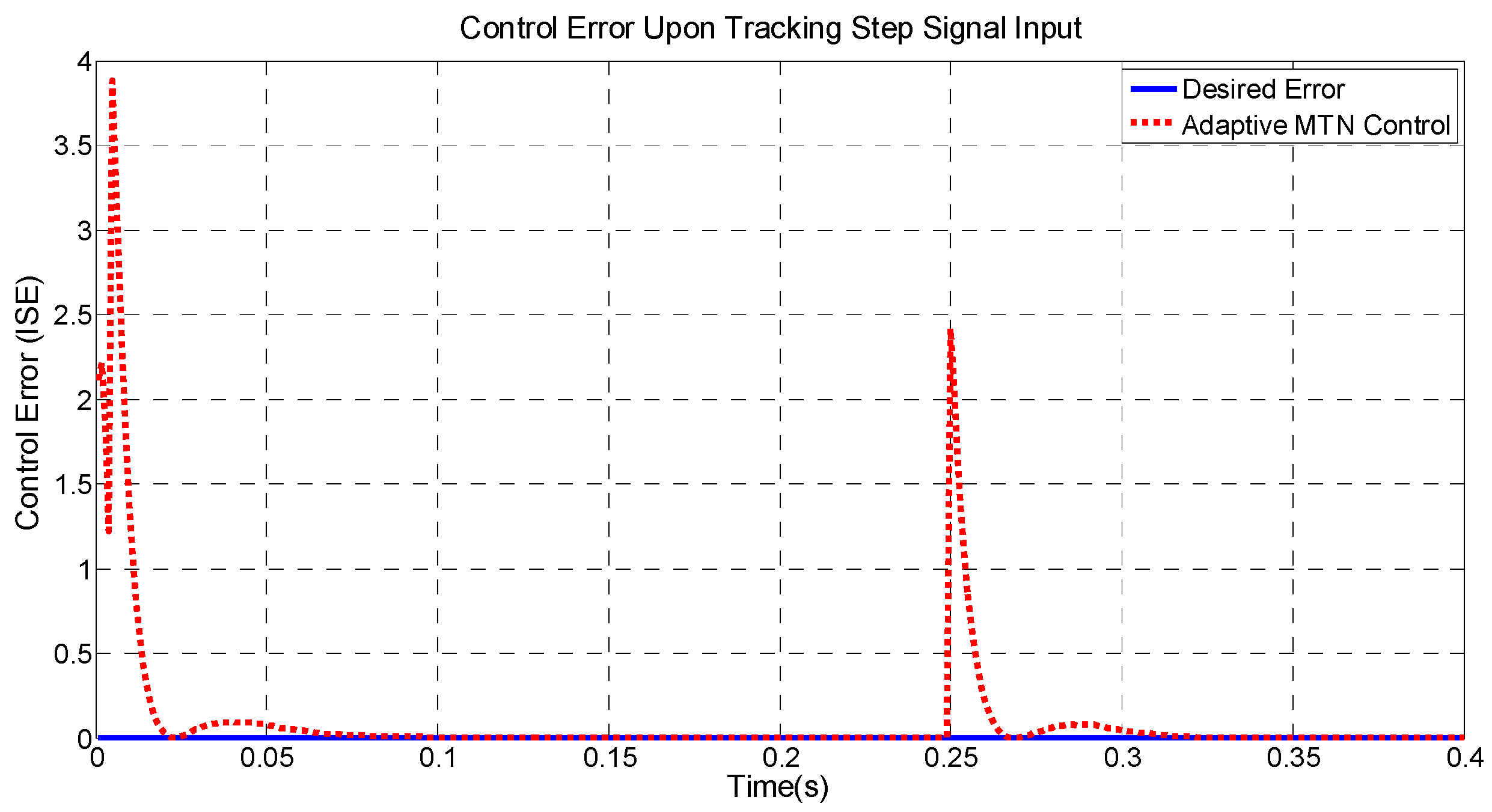
The control of the nonlinear MIMO time-varying system with measurement noises by an adaptive multi-dimensional Taylor network is simulated. Results are shown in Figure 6, Figure 7 and Figure 8. Figure 6 illustrates the contrast between the actual output and the object output by the two control methods. Figure 7 presents the control laws changing with time. Figure 8 gives the control error variation.

Figure 6. Comparison of responses between different control methods.

Figure 7. Control law variation.

Figure 8. Control error variation.

At 0.25 s, we increase the gains of $f_{11}(k)$ and $f_{22}(k)$ in Equation (30) by 25 times (i.e., $f_{11}(k)=53\left(1-e^{-0.6(k-1)}\right)$ and $f_{22}(k)=53\left(1-e^{-0.8(k-1)}\right)$. Tests conducted under time-varying conditions further validated the effectiveness of the proposed method. Through a comprehensive comparison of rise time, peak time, and settling time, MTN demonstrated a more significant improvement in control quality than neural networks in time-varying adaptive control.

For clear comparison, Table 3 lists the control errors over time, starting at 0.15 s. Fourteen sets of data were selected. Simulation results show that the actual output can quickly approximate the target output using the method proposed in this paper. The control error decreases faster until 0.02 s, after which it gradually tends to 0. Control laws also change into constants within a short time. For complex nonlinear systems, adaptive MTN controllers and filters have more desirable convergence speed, accuracy and stability.

Table 3. Control error comparison between RBFNN and MTN.

Groups	Times (s)	Adaptive RBFNN Control	Adaptive MTN Control
1	0.02	0.4854	0.0248
2	0.03	0.0336	0.0532
3	0.04	0.0111	0.0959
4	0.05	0.0522	0.0693
5	0.06	0.0760	0.0405
6	0.07	0.0798	0.0223
7	0.08	0.0720	0.0133
8	0.09	0.0594	0.0081
9	0.10	0.0451	0.0050
10	0.11	0.0340	0.0034
11	0.12	0.0252	0.0024
12	0.13	0.0170	0.0011
13	0.14	0.0116	0.0007
14	0.15	0.0088	0.0009
Mean	-	0.0674	0.0227

Note: ‘Times (s)’ denotes the sampling time points with a sampling interval of 0.01 s, consistent with the system parameter setting.

To quantify the trade-off between the MTN expansion order m and filtering performance, we conducted controlled simulation tests under completely consistent system parameters and noise conditions. The results are summarized in Table 4, which clearly identifies the accuracy saturation point.

Table 4. Trade-off between MTN expansion order m and filtering performance.

MTN Expansion Order m	Steady-State Mean Filtering Error	Error Reduction vs. m = 1	Single-Step Computational Load (FLOPs)
1	0.0892	Baseline	420
2 (Selected in this paper)	0.0227	74.5%	1180
3	0.0198	77.8%	2350
4	0.0191	78.6%	4120
5	0.0188	78.9%	6570

As shown in Table 4, filtering accuracy improves significantly with increasing m when m ≤ 3. When m > 3, the error reduction is less than 1.1% compared with m = 3, meaning the accuracy reaches the saturation point. Continuing to increase the expansion order cannot significantly improve accuracy, but will lead to a sharp rise in computational load. The m = 2 selected in this paper achieves the optimal balance between filtering accuracy and computational efficiency.

To verify the correctness of the above theoretical analysis, we conducted controlled simulation tests under three typical ${\kappa }_2$ values with consistent system parameters and noise conditions. The performance comparison results are summarized in Table 5.

Table 5. Filtering performance comparison under different ${\kappa }_2$ values.

${\mathit{\kappa }}_2$ Value	Steady-State Mean Error	Convergence Time (s)	Numerical Stability
10−5	0.0512 (with oscillation)	0.08	Unstable
10−3	0.0227	0.05	Stable
0.1	0.0812	0.12	Stable (with significant steady-state bias)

The results fully validate our theoretical analysis: an excessively small ${\kappa }_2$ leads to numerical instability, while an excessively large ${\kappa }_2$ introduces significant steady-state bias. The ${\kappa }_2$ value selected in this paper achieves the optimal balance of all core performance indicators.

On the basis of the steady-state performance verification under ideal white noise, we further conducted controlled simulation experiments to verify the robustness of the proposed LAF-MTNF against industrial common correlated noise, with the noise type as the only variable and all other system parameters completely consistent with the benchmark experiment. The filtering performance comparison under different noise scenarios is shown in Table 6.

Table 6. Filtering performance comparison under different types of correlated noise.

Noise Type	Steady-State Mean Error (LAF-MTNF)	Steady-State Mean Error (RBFNN-LAF)	Convergence Time of LAF-MTNF (s)
White Gaussian Noise (Reference)	0.0227	0.0674	0.05
Pink Noise (Correlation Coefficient 0.85)	0.0255	0.0992	0.06
Blue Noise (Correlation Coefficient 0.7)	0.0247	0.0863	0.055

The results quantitatively verify that the proposed LAF-MTNF maintains excellent filtering performance under both pink noise and blue noise: the steady-state error increases by less than 13% compared with the white noise scenario, and the convergence speed remains at a high level. In contrast, the benchmark RBFNN-LAF filter shows a significant performance degradation under correlated noise, with the steady-state error increasing by up to 47.2%. This fully validates the strong robustness of the proposed method against the correlated noise widely present in industrial sensors.

For the non-Gaussian impulsive noise widely existing in power systems, industrial transmission lines and switching circuits, we further conducted targeted robustness verification based on the same benchmark system. The impulsive noise model adopts the industrial widely recognized standard: the impulse amplitude is 5 times the standard deviation of the background Gaussian noise, and the random occurrence probability is 1% per sampling step, which fully matches the actual characteristics of impulsive disturbances in industrial power systems. The performance comparison results are summarized in Table 7.

Table 7. Filtering performance comparison under non-Gaussian impulsive noise.

Noise Scenario	Steady-State Mean Error (Proposed LAF-MTNF)	Steady-State Mean Error (RBFNN-LAF Benchmark)	Peak Overshoot of Filtering Error
Gaussian Noise Only	0.0227	0.0674	0.0812
Gaussian + Impulsive Noise	0.0286	0.1247	0.1526

The results show that under non-Gaussian impulsive noise, the steady-state error of the proposed LAF-MTNF only increases by 26.0% compared with the ideal Gaussian noise scenario, and the peak overshoot of the filtering error is effectively suppressed. In contrast, the RBFNN-LAF benchmark method suffers from serious performance degradation, with the steady-state error increasing by 85.0% and a large peak overshoot under impulse disturbances. This fully verifies that the proposed method has strong robustness to non-Gaussian non-stationary disturbances in industrial environments.

To verify the tight coupling handling capability of the proposed method, we conducted step disturbance tests on each input channel, and used the cross-coupling error (CCE) metric to quantify the influence of a single input change on other output estimates. The CCE of the j-th non-target output channel when the i-th input is disturbed is defined as ${\mathrm{CCE}}_{ij}=\left|{\widehat{y}}_j(k)-y_j(k)\right|$, where ${\widehat{y}}_j(k)$ is the filter’s estimated output and y_j is the real output. The test results are summarized in Table 8.

Table 8. Cross-coupling error comparison under input step disturbance.

Disturbed Input Channel	Method	CCE Peak of Non-Target Output	Steady-State CCE of Non-Target Output
Input Channel 1	Proposed LAF-MTNF	0.0241	0.0032
	RBFNN-LAF Benchmark	0.1186	0.0217
Input Channel 2	Proposed LAF-MTNF	0.0218	0.0028
	RBFNN-LAF Benchmark	0.1093	0.0195

The results show that the proposed method has an extremely low cross-coupling error, with steady-state CCE less than 0.4% of the full output range. A single input change will not erroneously affect the estimation of other outputs, which fully verifies its excellent tight coupling handling capability.

To further validate real-time applicability, we added real-time performance metrics to the simulation; we recorded the average computation time per iteration (for both controller and filter) based on 10,000 consecutive iterations on a PC platform (Intel Core i5-10400, 2.9 GHz), and compared the results between MTN and RBFNN.

As shown in Table 9, the MTN-based system not only has a lower average computation time but also a smaller jitter (delay variance)—a key indicator for real-time control (jitter > 0.2 ms may cause unstable system response in industrial scenarios). For the simulated MIMO system with a sampling interval of 0.01 s (100 Hz sampling frequency), the MTN’s maximum computation time (0.52 ms) is far less than the sampling interval, leaving sufficient margin for other real-time tasks (e.g., sensor data acquisition, communication). In contrast, the RBFNN’s maximum computation time (2.51 ms) occupies 25.1% of the sampling interval, increasing the risk of task blocking and control lag. This simulation result further confirms that MTN’s low computational complexity directly supports its real-time applicability in industrial control systems. The actual execution time advantage of the proposed method is fully consistent with the theoretical FLOPs comparison results in Table 1, which further verifies its superiority in real-time industrial control scenarios. Based on the verified total FLOPs per iteration and the official performance parameters of the STM32H743 industrial MCU (400 MHz Cortex-M7 core with hardware FPU), the theoretical single-step execution time of the proposed method is far less than the 1 ms sampling period commonly used in industrial control systems, showing significant theoretical real-time advantages for industrial embedded deployment. It should be noted that the actual embedded execution performance will be affected by engineering implementation factors such as compiler optimization level, peripheral interrupt scheduling, and hardware resource constraints. For resource-limited embedded platforms, additional engineering optimization measures are required to achieve the theoretical performance advantage.

Table 9. Real-time performance comparison between RBFNN and MTN (per iteration).

Metric	Adaptive RBFNN (Controller + Filter)	Adaptive MTN (Controller + Filter)	Reduction Ratio
Average Computation Time	1.82 ms	0.35 ms	~80.8%
Maximum Computation Time	2.51 ms	0.52 ms	~79.3%
Delay Variance (Jitter)	0.36 ms2	0.08 ms2	~77.8%

While simulation results (Section 5) validate LAF-MTNF’s efficacy under controlled nonlinear MIMO scenarios, real-world deployment requires addressing practical challenges—these challenges also point to key directions for future research.

Parameter Initialization for Hardware Adaptation: The offline inverse modeling of MTN controller weights (Section 3) relies on sufficient training samples (e.g., white noise signals). In real systems (e.g., permanent magnet synchronous motors, industrial robots), variations in hardware parameters (e.g., motor inertia, robot joint friction) may require adaptive initialization strategies (e.g., transfer learning-based sample augmentation) to avoid time-consuming retraining.

Real-Time Performance Trade-Off: The approximation accuracy of MTN is determined by the number of expansion terms $N(n,m)$ (Equation (3)), creating a trade-off between precision and computational efficiency. For high-speed systems (e.g., power grid frequency regulation, motor speed control), increasing $N(n,m)$ to enhance filtering precision will inevitably increase computational latency. Future work could explore hardware acceleration (e.g., FPGA implementation) or sparse MTN structures to balance precision and real-time responsiveness.

Robustness to Non-Gaussian Noise: The simulation uses white Gaussian noise (mean 0, std 0.05), but real industrial environments often involve non-Gaussian noise (e.g., impulsive noise in power systems). Extending LAF-MTNF to non-Gaussian scenarios (e.g., integrating robust statistics into the Lyapunov function) would enhance its practical applicability.

Despite these challenges, LAF-MTNF’s simplicity (linear parameterization of MTN) and stability (LST guarantee) make it a promising candidate for real-world nonlinear MIMO systems, especially those requiring reliable denoising and fast adaptation (e.g., intelligent manufacturing equipment, unmanned vehicle control).

For high-dimensional MIMO systems with more than 3 inputs/outputs, future work will explore hardware acceleration (e.g., FPGA implementation) and sparse MTN structure optimization based on contribution pruning, to further balance approximation accuracy and real-time responsiveness in ultra-high-dimensional industrial scenarios such as 6-axis collaborative robots and 5-axis CNC machining centers.

6. Conclusions

In this study, we propose an adaptive multi-dimensional Taylor network filter (LAF-MTNF) integrated with Lyapunov stability theory (LST), which addresses three critical limitations of existing methods and advances the field of MIMO time-varying uncertain nonlinear system filtering.

(1)

Unlike existing MTN-based filters that rely on LMS/RLS weight-update algorithms—which are prone to local minima and lack stability guarantees—our LST-based weight adaptation scheme constructs an energy space with a single global minimum, eliminating local optimization traps and ensuring asymptotic stability (Theorem 1). This fills the gap of “stability–optimization decoupling” in traditional MTN filtering.

(2)

Compared with Lyapunov-based filters (e.g., LST-RBFNN) that face unresolved issues of RBF node center/Gaussian width selection and incomplete convergence analysis, we provide a systematic quantification of convergence performance: we derive explicit expressions for the error convergence rate (regulated by the positive constant) and convergence region (a sphere centered at the origin with radius defined in Equation (14)) while modifying the adaptive gain (Equation (12)) to avoid singularity. This completes the theoretical framework of Lyapunov-based filtering for complex MIMO systems.

(3)

Unlike adaptive filters that require prior knowledge of noise statistics, our LAF-MTNF only uses input/output measurements and is disturbance-independent, making it more robust to unknown measurement noise in industrial scenarios.

Simulation results further validate that LAF-MTNF outperforms RBFNN-based filters in control accuracy (mean error 0.0227 vs. 0.0674, Table 3) and dynamic response (faster convergence to near-zero error), confirming its superiority in handling strong coupling, time variation, and random disturbances.

In conclusion, this work makes two key contributions to the field of adaptive filtering for nonlinear MIMO systems: theoretically, it integrates LST with MTN to establish a stable, disturbance-independent filtering framework, filling gaps in convergence quantification and stability analysis of existing methods; practically, it provides a low-complexity, real-time applicable alternative to RBFNN-based filters. (1) MTN’s computational load is only ~6.2% of RBFNN (296 vs. 2376 FLOPs), ensuring <1 ms per iteration on industrial MCUs; (2) simulation shows that MTN reduces computation time by ~80.8% and jitter by ~77.8% compared to RBFNN, meeting the real-time requirements of 100 Hz–5 kHz industrial sampling frequencies; (3) adjustable expansion terms and FPGA acceleration support flexible trade-offs between precision and real-time performance. The proposed algorithm only requires the measurement noise to be bounded, with no strict statistical assumptions on the noise, which greatly reduces the constraints for practical industrial deployment, and shows strong robustness to various non-ideal industrial noise processes. These features make LAF-MTNF particularly suitable for highly dynamic real-time scenarios, such as permanent magnet synchronous motor control, industrial robot trajectory tracking, and power grid frequency regulation. By addressing the tension between stability, precision, and adaptability in complex systems, LAF-MTNF lays a foundation for future research on MTN-based control in real-world industrial applications.

References

- Yang, Y.; Zhang, H.H. Optimal model reference adaptive fractional-order proportional integral derivative control of idle speed system under varying disturbances. Proc. Inst. Mech. Eng. Part I J. Syst. Control Eng. 2025, 239, 339–355. [Google Scholar] [CrossRef] [Scilit]
- Zhong, H.; Liu, K.; Qiang, H.; Yang, J.; Kang, S. Model reference adaptive control of electro-hydraulic servo system based on RBF neural network and nonlinear disturbance observer. Proc. Inst. Mech. Eng. Part I J. Syst. Control Eng. 2025, 239, 535–549. [Google Scholar] [CrossRef] [Scilit]
- Cai, M.; He, X.; Zhou, D. Low-power fault-tolerant control for nonideal high-order fully actuated systems. IEEE Trans. Syst. Man Cybern. Syst. 2023, 53, 4875–4887. [Google Scholar] [CrossRef] [Scilit]
- Wan, M.; Song, J.; Wang, G. Observer-based adaptive fuzzy control of stabilized platform in rotary steerable system with input saturation and output constraint. Proc. Inst. Mech. Eng. Part I J. Syst. Control Eng. 2024, 238, 1785–1799. [Google Scholar] [CrossRef] [Scilit]
- Liu, J.; Gong, E.; Zha, L.; Tian, E.; Xie, X. Observer-based security fuzzy control for nonlinear networked systems under weighted try-once-discard protocol. IEEE Trans. Fuzzy Syst. 2023, 31, 3853–3865. [Google Scholar] [CrossRef] [Scilit]
- Dong, S.; Liu, M. Adaptive fuzzy asynchronous control for nonhomogeneous Markov jump power systems under hybrid attacks. IEEE Trans. Fuzzy Syst. 2022, 31, 1009–1019. [Google Scholar] [CrossRef] [Scilit]
- Dinçmen, E. Neural network steering control algorithm for autonomous ground vehicles having signal time delay. Proc. Inst. Mech. Eng. Part I J. Syst. Control Eng. 2024, 238, 720–736. [Google Scholar] [CrossRef] [Scilit]
- Paszkowiak, W.; Pelic, M.; Bartkowiak, T. A neural-network-based control system for a dynamic model of tractor with multiple trailers system. Int. J. Control Autom. Syst. 2023, 21, 3456–3469. [Google Scholar] [CrossRef] [Scilit]
- Darvishzadeh, A.; Iman-Eini, H.; Neyshabouri, Y. Diagnosis and ride through of single-switch open-circuit fault in low-capacitance STATCOM. IEEE Trans. Power Electron. 2025, 40, 1952–1963. [Google Scholar] [CrossRef] [Scilit]
- Merrikh-Bayat, F.; Mirhoseini, P. On transforming hybrid nonlinear control problems with model uncertainty and input disturbance to mixed integer-linear programs. J. Frankl. Inst. 2023, 360, 14406–14415. [Google Scholar] [CrossRef] [Scilit]
- Zhang, C.; Yan, H.S. Identification and adaptive multi-dimensional Taylor network control of single-input single-output non-linear uncertain time-varying systems with noise disturbances. IET Control Theory Appl. 2019, 13, 841–853. [Google Scholar] [CrossRef] [Scilit]
- Zhang, C.; Yan, H.S. Inverse control of multi-dimensional Taylor network for permanent magnet synchronous motor. COMPEL Int. J. Comput. Math. Electr. Electron. Eng. 2017, 36, 1676–1689. [Google Scholar] [CrossRef] [Scilit]
- Zhang, C.; Yan, H.S. Multidimensional Taylor network adaptive control for MIMO time-varying uncertain nonlinear systems with noises. Int. J. Robust Nonlinear Control 2020, 30, 397–420. [Google Scholar] [CrossRef] [Scilit]
- Trinh, M.H.; Pham, Q.D.; Giap, V.N. Optimal Lyapunov-based sliding mode control for slotless-self bearing motor system. Appl. Syst. Innov. 2022, 6, 2. [Google Scholar] [CrossRef] [Scilit]
- Kuzenov, V.V.; Ryzhkov, S.V.; Varaksin, A.Y. Development of a method for solving elliptic differential equations based on a nonlinear compact-polynomial scheme. J. Comput. Appl. Math. 2024, 451, 116098–116121. [Google Scholar] [CrossRef] [Scilit]
- Jin, Z.H. Global asymptotic stability analysis for autonomous optimization. IEEE Trans. Autom. Control 2025, 70, 6953–6960. [Google Scholar] [CrossRef] [Scilit]
- Wang, Y.T.; Jin, Z.H.; Jiang, Y. Adaptive event-triggered control for a class of nonlinear systems with unknown time-varying parameters. Automatica 2026, 184, 112703–112712. [Google Scholar] [CrossRef] [Scilit]
- Song, X.Y.; Wu, H.; Wang, Z.; Zou, Y.; Sa, X.; Zhao, Z. A Review of Control Techniques for Imbalance-Induced Vibration in Magnetically Suspended Rotor Systems. Appl. Sci. 2025, 15, 13249. [Google Scholar] [CrossRef] [Scilit]
- Zhang, G.Q.; Peng, M.G.; Zhang, W.Q.; Pan, M.; Xu, Z.; Zheng, J. Advances in monitoring system and application in precision/ultra-precision machining processes. Int. J. Adv. Manuf. Technol. 2025, 140, 5823–5868. [Google Scholar] [CrossRef] [Scilit]
- Zhang, Y.; Zhang, K.; Ghazal, A.; Zhang, W.; Ji, Z.; Xiao, L. Non-stationarity characterization and geometry-cluster-based stochastic model for high-speed train radio channels. IEEE Trans. Intell. Transp. Syst. 2023, 24, 7122–7137. [Google Scholar] [CrossRef] [Scilit]
- Song, Z.; Li, P. General Lyapunov stability and its application to time-varying convex optimization. IEEE/CAA J. Autom. Sin. 2024, 11, 2316–2326. [Google Scholar] [CrossRef] [Scilit]
- Lim, K.H.; Seng, K.P.; Ang, L.M.; Chin, S.W. Lyapunov theory-based multilayered neural network. IEEE Trans. Circuits Syst. II Express Briefs 2009, 56, 305–309. [Google Scholar]
- Cui, M.; Liu, H.; Li, Z.; Tang, Y.; Guan, X. Identification of Hammerstein model using functional link artificial neural network. Neurocomputing 2014, 142, 419–428. [Google Scholar] [CrossRef] [Scilit]
- Shi, Z.; Yang, H.; Dai, M. The data-filtering based bias compensation recursive least squares identification for multi-input single-output systems with colored noises. J. Frankl. Inst. 2023, 360, 4753–4783. [Google Scholar] [CrossRef] [Scilit]
- Yadav, N.K.; Dhawan, A.; Tiwari, M.; Jha, S.K. A state-of-the-art survey on noise removal in a non-stationary signal using adaptive finite impulse response filtering: Challenges, techniques, and applications. Int. J. Syst. Sci. 2025, 56, 885–918. [Google Scholar] [CrossRef] [Scilit]
- Ye, J.; Yu, Y.; Cai, Q.; Yu, T.; Chen, B. P-norm based subband adaptive filtering algorithm: Performance analysis and improvements. Circuits Syst. Signal Process. 2024, 43, 1208–1239. [Google Scholar] [CrossRef] [Scilit]
- Klambauer, G. Mathematical Analysis Vol. 31; Marcel Dekker INC: New York, NY, USA, 1975. [Google Scholar]
- Li, C.L.; Li, W.S.; Zhang, Z.J. Composite anti-disturbance predictive control of unmanned systems with time-delay using multi-dimensional Taylor network. Chin. J. Aeronaut. 2025, 38, 103279–103290. [Google Scholar] [CrossRef] [Scilit]
- Treesatayapun, C. Prescribed performance of discrete-time controller based on the dynamic equivalent data model. Appl. Math. Model. 2020, 78, 366–382. [Google Scholar] [CrossRef] [Scilit]
- Er, M.J.; Gong, H.; Liu, Y.; Liu, T. Intelligent trajectory tracking and formation control of underactuated autonomous underwater vehicles: A critical review. IEEE Trans. Syst. Man Cybern. Syst. 2023, 54, 543–555. [Google Scholar] [CrossRef] [Scilit]
- Golub, G.H.; Van Loan, C.F. Matrix Computations Vol. 3; JHU Press: Baltimore, MD, USA, 2012. [Google Scholar]
- Rahmani, Z.; Baigzadehnoe, B.; Rezaie, B. Tracking control of a class of nonlinear systems with output delay based on adaptive fuzzy dynamic surface control. Int. J. Syst. Sci. 2020, 51, 1280–1306. [Google Scholar] [CrossRef] [Scilit]
Disclaimer/Publisher’s Note: The statements, opinions and data contained in all publications are solely those of the individual author(s) and contributor(s) and not of MDPI and/or the editor(s). MDPI and/or the editor(s) disclaim responsibility for any injury to people or property resulting from any ideas, methods, instructions or products referred to in the content. |
© 2026 by the authors. Published by MDPI on behalf of the International Institute of Knowledge Innovation and Invention. Licensee MDPI, Basel, Switzerland. This article is an open access article distributed under the terms and conditions of the Creative Commons Attribution (CC BY) license.