


Abstract
The increasing penetration of non-conventional renewable energy sources poses operational flexibility challenges that motivate the coordination of distributed energy resources via active demand management. This study proposes an optimal operational strategy for a Virtual Power Plant (VPP) integrating conventional thermal generation, renewable sources, battery energy storage, main grid transactions, and active demand mechanisms. The optimization model is formulated as a Mixed-Integer Linear Programming (MILP) problem embedded within a receding horizon Model Predictive Control (MPC) framework. Active demand is represented through an aggregated shiftable load and distinct curtailable loads. Shiftable-load operation is regulated through power, ramping, and energy-balance constraints, whereas curtailable loads are governed by user discomfort penalties, economic incentives, and daily curtailment budgets. Renewable forecasting uncertainties are mitigated using a hybrid physical-LSBoost model that reduces prediction errors by up to 93.0%. Operational results demonstrate total operating cost reductions ranging from 2.08% to 15.34%, alongside an 8.65% peak demand reduction. A comprehensive sensitivity analysis reveals that active demand participation is governed by distinct qualitative mechanisms: strict budget bounds, a steep penalty threshold for curtailment activation, and a threshold-type saturation response to temporal price spreads for shiftable loads. Furthermore, high-resolution 5-min online operation confirms the real-time viability of the scheme, maintaining solver execution times under 1.69 s per iteration. It is concluded that coordinating active demand, storage, and MPC enhances both economic and technical VPP performance, though carbon emission abatement relies heavily on thermal dispatch dynamics, highlighting the need to explicitly balance economic and environmental trade-offs.
1. Introduction
1.1. Context
The energy transition toward more sustainable power systems is characterized by the growing penetration of non-conventional renewable energy sources (NCRES), particularly wind and photovoltaic generation [1]. These technologies contribute significantly to the decarbonization process; however, their variable and uncertain nature, linked to their dependence on environmental conditions, poses major challenges for power system operation [2]. Among these challenges are the need for higher levels of operational flexibility, the development of effective demand-side management mechanisms, and the implementation of advanced power dispatch planning schemes.
In addition, the development of smart grids and the growing adoption of distributed energy resources (DER), such as distributed generation, energy storage systems, and controllable loads, have given rise to new management architectures and the consolidation of more dynamic business models worldwide. These developments are increasingly supported by regulatory frameworks that recognize both the role of non-conventional renewable energy sources and the active participation of end users as key elements of the energy transition [3].
In response to these challenges, the concept of a virtual power plant (VPP) has emerged as an alternative for coordinating and optimizing the operation of multiple DERs. A VPP operates as an aggregation platform that integrates generation units (photovoltaic, wind, or conventional), energy storage systems, and various types of flexible loads, enabling the resources to behave collectively as a single, manageable entity [4]. Its main objectives include minimizing operating costs, reducing emissions, increasing the utilization of renewable sources, and improving the flexibility of the power system [5].
Active demand plays a fundamental role and is implemented through demand response (DR) programs, which can be classified into price-based demand response (PBDR) and incentive-based demand response (IBDR) programs [6]. Traditionally, electricity demand is considered inelastic, with fixed and uncontrollable consumption profiles. However, the active demand approach seeks to manage certain loads, either in time or in magnitude, by taking advantage of the flexibility of different types of loads, such as shiftable loads, which can be rescheduled within a given time window, and curtailable loads, which can temporarily decrease their power [7]. The integration of these behaviors into the VPP model is of interest for optimizing the energy supply and using power demand as an additional resource to improve the economic and technical efficiencies of the power system.
1.2. Literature Review
Recent literature highlights numerous VPP management architectures. Li et al. [8] presented an operating strategy for a low-carbon VPP that integrates wind and photovoltaic generation, gas turbines, battery energy storage systems, and flexible loads classified as shiftable and reducible. The model incorporates a progressive demand response mechanism, as well as a carbon trading scheme and an emissions intensity index. Using day-ahead scheduling, the VPP optimizes the generation dispatch and demand response activation to minimize the total operating cost and CO2 emissions. The simulation results show that the progressive demand response strategy slightly increases the total system cost (0.58%), but reduces the cost associated with carbon emissions by approximately 20.35% and improves the load profile. However, although the model considers day-ahead and intraday dispatch schemes on multiple time scales, it is not explicitly formulated as a real-time control scheme and does not include the cost associated with user comfort.
However, Zhou et al. [9] proposed an urban VPP that integrates diesel generation, photovoltaic generation, energy storage systems, and electricity buy-and-sell prices in the wholesale market. This study proposed a bi-level model that incorporates incentive-based demand response programs. The process was divided into two layers. In the lower layer, an IDR model is formulated that considers user satisfaction, comfort, and preferences using reinforcement learning (Q-learning) to adaptively adjust the individual incentive tariff and maximize the joint benefit of the VPP and the users. In the upper layer, an hourly optimal dispatch problem is solved that determines the operation of distributed resources and market transactions, with the objective of minimizing the operating cost of the VPP. The simulation results, based on real data for demand, prices, and photovoltaic generation, show that the incorporation of IBDR programs reduces aggregate demand by approximately 28% and decreases the operating cost of the VPP by approximately 19% compared to a scenario without active user participation. However, although the model incorporates demand response mechanisms and considers user satisfaction in an aggregated manner, its formulation is posed as a static dispatch problem over a fixed scheduling horizon, without an explicit classification of the different types of flexible loads or the inclusion of terms associated with carbon emissions.
The analysis of these studies highlights the need for energy management models that consider the use of VPPs. As structures, they do not strictly depend on a physical network topology, as their virtual nature allows them to coordinate distributed resources to support the stability and efficiency of the power system without requiring direct physical integration into the transmission or distribution systems. Similarly, it is essential that these models incorporate strategies that consider the needs, preferences, and consumption profiles of users to design demand response programs that achieve a balance between energy efficiency and user comfort. Finally, the operation and analysis of these models must be addressed in near-real-time scenarios, which helps improve optimization and dispatch processes by explicitly considering the variability and uncertainty associated with generation, demand, and electricity market prices.
Despite these advancements, managing VPPs under near-real-time grid conditions requires robust control frameworks capable of absorbing continuous forecast errors. MPC has demonstrated high effectiveness in handling operational stochasticity through receding-horizon control (RHC) [10]. Bustos Marambio, R.I.B. et al. [11] demonstrated that hierarchical energy management systems (EMS) based on MPC, with the incorporation of demand management, can reduce operating costs and improve the utilization of renewable sources in multi-microgrid systems. Nevertheless, this model focuses on aggregated demand-shifting strategies and does not explicitly consider the participation of a VPP in the electricity market, detailed classification of flexible loads, or inclusion of the cost associated with CO2 emissions in the objective function.
Similarly, Chang et al. [12] developed a collaborative energy management framework for a VPP aggregated from multiple microgrids, in which a stochastic day-ahead dispatch was combined with a real-time continuous dispatch scheme based on receding horizon MPC and a penalty mechanism for forecast errors. However, the model does not address the detailed characterization of flexible loads on the demand side, nor does it include terms associated with potential user discomfort.
Beyond VPP-specific studies, related work on coordinated scheduling of flexible demand and storage in adjacent domains further illustrates the methodological landscape. Li et al. [13] propose a collaborative response framework coordinating data center workload flexibility with a hydrogen storage system to absorb excess renewable generation, addressing the resulting non-convex, NP-hard optimization problem through a global interval optimization (GIO) approach that achieves robust decisions under uncertain renewable supply. While this work demonstrates an alternative storage-coupled flexibility mechanism, it targets a fundamentally different demand-side context (data center workload) and does not address cost-based user discomfort, carbon emission costs, or a receding horizon control scheme. Similarly, Dong et al. [14] propose a safe, AutoML-enhanced deep reinforcement learning approach (Safe-AutoSAC) for integrated energy system scheduling with electric vehicle demand response, incorporating a multi-channel Informer forecasting model with cross-channel attention to improve renewable and load prediction accuracy. This learning-based approach offers adaptability to complex, high-dimensional uncertainty without requiring an explicit mathematical formulation of the system dynamics, in contrast to the MILP-MPC approach adopted in this work; however, it does not provide the optimality guarantees (within a defined MIP gap) that characterize mathematical programming approaches, and its training and safety-assurance mechanisms introduce additional implementation complexity. These two studies illustrate two methodologically distinct alternatives—robust interval optimization and safe deep reinforcement learning—to the MILP-MPC framework adopted in this work, motivating the discussion of trade-offs between optimization paradigms presented in Section 2.
This study presents the following contributions based on the literature review.
- An optimal dispatch model is proposed for a VPP that integrates renewable generation, conventional generation units, energy storage systems, and interaction with the distribution grid within a single optimization framework.
- Active participation of demand is generally incorporated through the implementation of price- and incentive-based demand response programs.
- The objective function incorporates cost components associated not only with energy and resource operation, but also with demand flexibility, carbon emission reduction, and possible user discomfort.
- The performance of the model is evaluated under near-real-time operating conditions, explicitly taking into account the variability of renewable generation.
2. VPP Methodology and Architecture
2.1. General Architecture of the VPP
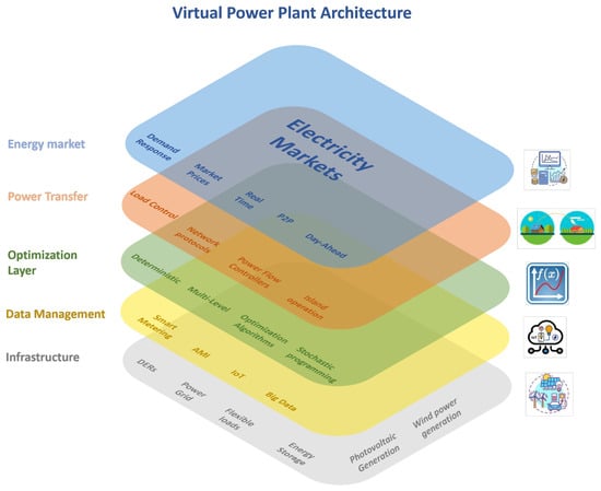
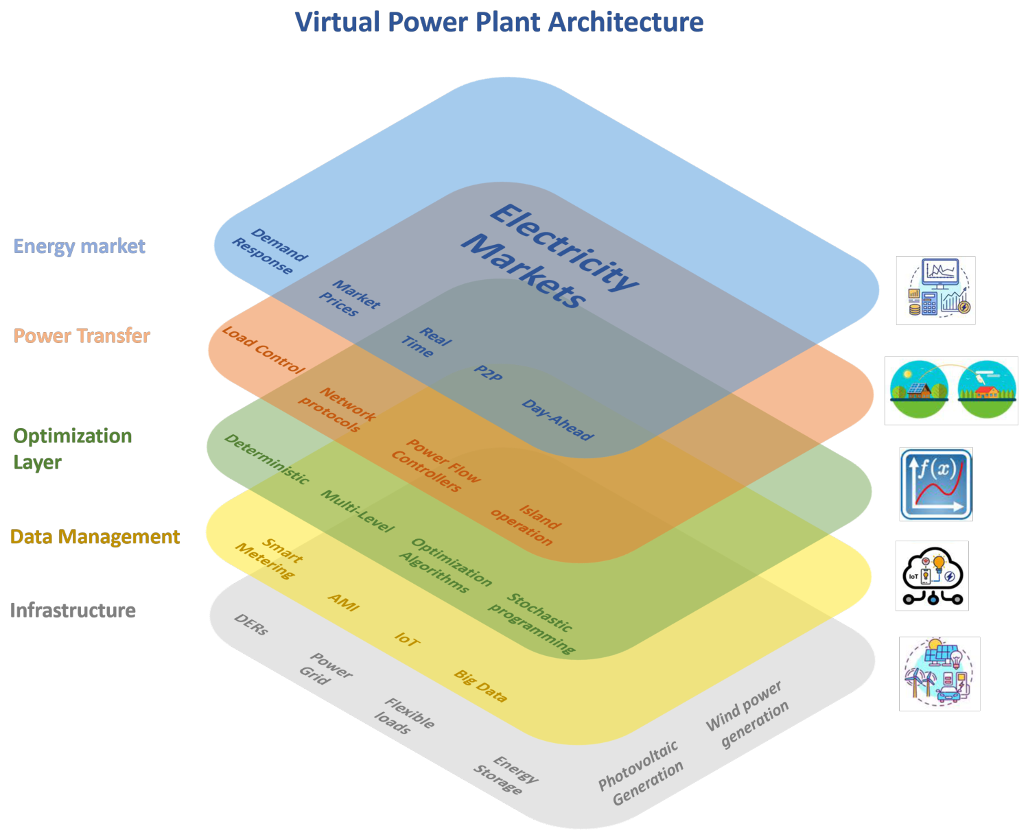
VPPs can be understood as a layered architecture that hierarchically coordinates distributed energy resources, measurement and communication systems, optimization algorithms, and interaction with electricity markets. This architecture helps separate the physical, communication, decision-making, and market functions, enabling the modular design and implementation of each component. In this study, five main functional layers were considered:
Infrastructure. This layer includes distributed energy resources (photovoltaic and wind generation, thermal units, storage systems, flexible loads, and potentially electric vehicles), as well as the distribution network and metering devices. This layer represents the physical assets on which the VPP is operated.
Data management. This layer groups together the systems for data acquisition, transmission, storage, and preprocessing from the infrastructure, such as smart metering (AMI), SCADA systems, IoT platforms, and historical databases. This layer also includes demand and renewable energy generation forecasting models, which are fed into the optimization layer [15].
Optimization layer. This is responsible for formulating and solving power dispatch and resource management problems. Here, the MILP model is coupled with the MPC strategy. In addition, it is implemented for the coordination of generation, storage, and active demand, considering the technical constraints of the network and the economic and environmental costs [16].
Power transfer. This layer executes the decisions obtained through the power flow controllers, inverters, switches, and grid automation devices. It coordinates the connection and disconnection of resources, the exchange of energy with the grid, and the application of instructions to the smart loads.
Electricity market. The top layer represents the interaction of the VPP with electricity markets and demand response programs. Here, the electricity buy and sell prices are managed, as well as DR incentives and participation in different scheduling horizons (day-ahead, intraday, or near-real-time scenarios) [17].
Figure 1 schematically summarizes these five layers and highlights the most relevant elements considered in the model developed in this thesis.
Figure 1.
General architecture of a VPP organized into five functional layers.
2.2. MPC Control Scheme for the VPP
The VPP coordinates the energy demand of a user group comprising flexible loads . These loads represent smart end-use devices capable of curtailing consumption or rescheduling operations to alternative time intervals, provided that such actions reduce the overall system operational cost while meeting minimum user comfort criteria.
The VPP operation is formulated over a discrete planning horizon , with hourly steps representing a standard operational day. At each control step , the central coordination unit receives renewable generation forecasts alongside pre-established baseline demand and market price profiles across a shrinking prediction horizon of length . This horizon contracts progressively toward the end of the day to prevent forecasts beyond the daily operational boundary.
To clarify the operational mechanics of the proposed MPC framework, the main formulation elements are defined as follows:
- State vector: , representing the battery state-of-charge, the remaining daily curtailment budget, and the cumulative energy inventory shifted by shiftable loads, respectively.
- Inputs at step k: Baseline demand profiles and market prices (), alongside available solar photovoltaic and wind power forecasts ().
- Receding horizon update mechanism: At each control step k, the optimization problem is solved over the prediction window . Only the first control action is implemented, and the state vector updates according to:where is reset to its initial daily allowance exclusively at the end of the daily dispatch period (), thereby preventing inadvertent budget replenishment within the intermediate prediction windows.
Through this receding horizon mechanism, the VPP serves as an active aggregator of supply- and demand-side assets, seeking cost-effective operation while limiting conventional thermal generation, grid interaction reliance, and user discomfort penalties.
2.3. Receding Horizon MPC Scheme and Time Scaling
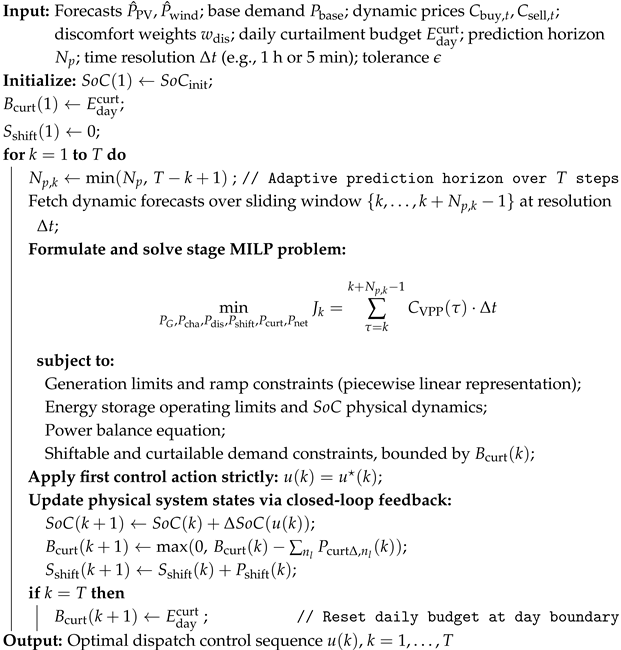
To clarify the operational implementation of the control scheme, it is important to note that the VPP does not simply solve a sequence of static and independent MILP problems over time. Instead, it executes a closed-loop receding horizon control scheme, as presented in Algorithm 1.
| Algorithm 1 MPC RHC Energy Management for VPP |
 |
- 1.
- Flexible time resolution (Δt): The scheme is evaluated under two operational time scales: an hourly resolution ( h, ), suitable for day-ahead scheduling, and an online resolution ( min, ), aimed at intraday balancing and absorbing fast variations in renewable generation.
- 2.
- Adaptive dynamic horizon: At each discrete control step k, the prediction horizon length is dynamically adjusted near the closure of the daily horizon T, incorporating updated short-term forecasts and .
- 3.
- Stage-wise optimization: The MILP engine minimizes the operating cost function over the active sliding window .
- 4.
- Closed-loop state update of the prediction scheme: Only the first control action is applied at each step. The state variables—the battery state of charge , the remaining reduction budget , and the cumulative inventory of shifted load —are deterministically updated from this applied action, consistently propagated to the next control step. In contrast, renewable generation variables are forecasted and then contrasted against independent measurements at each iteration (Section 2.4).
- 5.
- Continuity of the daily budget: At , the reduction budget is strictly reset to , establishing the conceptual basis for a potential extension of the model to multi-day operational horizons.
By combining receding horizon optimization with the periodic update of renewable generation forecasts, the MPC scheme effectively absorbs deviations between forecasted and measured generation, both at hourly and 5-min resolutions, as evidenced in the results of Section 5.
2.4. Forecasting Models and Uncertainty Characterization
2.4.1. Hybrid PV Generation Forecasting Model
To supply reliable photovoltaic generation forecasts to the VPP energy management system, a hybrid forecasting architecture combining a physical irradiance-to-power conversion model with a Machine Learning (ML) correction layer based on Least-Squares Boosting (LSBoost) was implemented. This hybrid structure captures the fundamental physical relationships of solar energy conversion while leveraging ML to dynamically offset systematic model errors and meteorological deviations.
The initial stage computes a physical power estimation based on solar geometry, plane-of-array irradiance (GHI, DNI, DHI), ambient temperature, and PV array tilt/orientation parameters. Following physical model calibration against historical microgrid telemetry, the forecast residual is defined as:
where represents the calibrated physical output and is the actual measured PV generation.
The residual serves as the target output for the LSBoost model, utilizing past meteorological measurements and temporal indices as feature predictors. The final hybrid forecast is computed by coupling the physical baseline with the predicted residual , bounded within physical inverter bounds:
Data splitting was executed chronologically—utilizing initial historical sequences for model training and subsequent unseen periods for validation—preventing future information leakage.
The model was evaluated across two operational time resolutions: a high-resolution 5-min timestep designed for intra-day closed-loop MPC dispatch, and an hourly resolution for daily market scheduling. As summarized in Table 1, the hybrid approach drastically reduces mean absolute error (MAE) and root mean square error (RMSE) compared to standalone physical modeling.
Table 1.
Performance metric comparison between physical and hybrid PV forecasting models.
2.4.2. Wind Generation Stochastic Modeling
The synthetic wind power profile is constructed by perturbing a deterministic baseline profile with a first-order autoregressive AR(1) multiplicative noise process normalized to unit variance:
The model parameters were set to an autocorrelation coefficient and a relative standard deviation (representing a 9% fluctuation relative to the baseline profile). This parameterization preserves realistic temporal auto-correlations between consecutive time steps, eliminating unrealistic uncorrelated white-noise spikes. For exact numerical reproducibility, the pseudo-random number generator seed was held constant across all simulation runs.
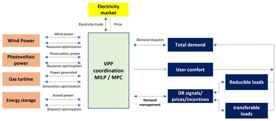
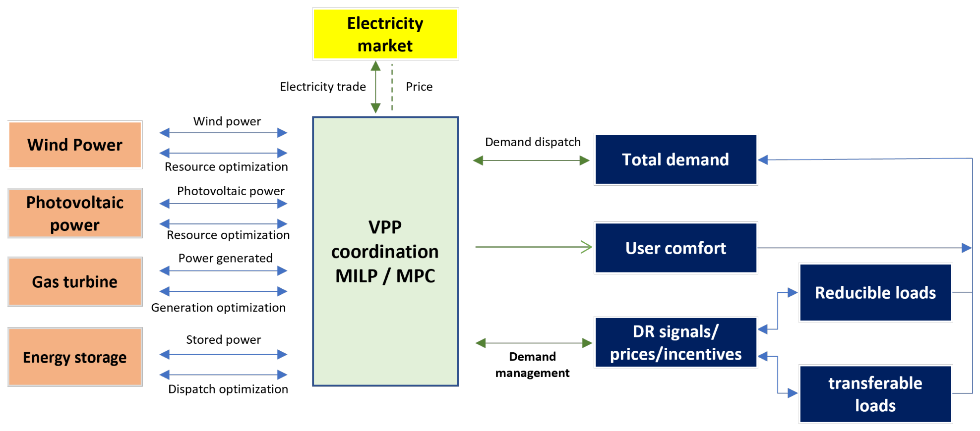
The complete structure of the system managed by the VPP is illustrated in Figure 2, where the generation sources, storage system, flexible demand, and interaction with the electricity market are explicitly shown, as well as the role of the central coordinator in solving the dispatch problem. This algorithm briefly describes the methodology for implementing and solving the optimization problem, focusing on MPC-based dispatch with a receding horizon control.
Figure 2.
General scheme of the proposed VPP, which integrates renewable generation, conventional units, storage, flexible demand, and its interaction with the electricity market. The VPP coordinator solves an optimization problem (MILP/MPC) that considers operating costs, CO2 emissions, and comfort-related aspects associated with user participation in demand response programs.
3. Mathematical Model
The mathematical formulation presented in this section builds upon the VPP energy management framework previously developed by the authors in [18], where model predictive control was applied to VPP energy dispatch. The present work extends this framework by integrating active demand response mechanisms, including price-based and incentive-based demand response, flexible loads and their associated economic costs, as well as a piecewise-linear formulation of thermal generation costs [19].
3.1. Cost Function
Equation (8) presents the objective function related to the minimum operating cost of VPP.
The term corresponds to the operation cost of the VPP and is expressed as in Equation (9).
The term is the cost associated with the maintenance of renewable generation, and is the generation cost of the thermal plant; is the cost attributed to the electricity buy and sell transactions with the power grid; is the cost generated by the carbon emissions produced by the gas turbines; and is the cost associated with the implementation of the DR program.
As summarized in Table 2, the objective function is composed of several cost terms. Each of these components is described in detail in Section 3.2.
Table 2.
Summary of objective function components and their dependencies.
3.2. Operation Cost
Next, the cost components associated with the operation of the different resources that constitute the VPP are described as follows.
3.2.1. Renewable Energy
For renewable energy sources, the operating cost is defined in Equation (10).
Here, t denotes the specific scheduling period. The terms , and represent the operation and maintenance costs of the wind turbines, photovoltaic systems, and batteries, respectively. The terms refer to the output powers of the wind turbines, photovoltaic systems, and batteries, respectively.
3.2.2. Thermal Generation Cost
The fuel cost of each gas turbine is inherently quadratic in its output power and is initially represented as in Equation (11).
where denotes the power output of gas turbine i at time t, while , , and are the corresponding quadratic, linear, and constant cost coefficients, respectively. Since the quadratic term would result in a mixed-integer quadratic programming (MIQP) formulation, the generation cost is reformulated using a piecewise-linear approximation to preserve the MILP structure of the overall optimization problem. The proposed piecewise-linear formulation is described in Section 3.2.3. The resulting thermal generation cost is expressed in Equation (12).
The term is a binary variable indicating the commitment status of generator i at time t; is the fixed generation cost associated with the minimum operating output; K is the number of linear segments used to approximate the quadratic fuel-cost curve; is the slope of segment k, calculated from the secant connecting its two adjacent breakpoints; and is the incremental power dispatched within segment k of generator i at time t. The parameters and denote the startup and shutdown costs of generator i, respectively, while and are binary variables indicating the corresponding startup and shutdown states.
3.2.3. Piecewise-Linear Approximation of Generation Cost
Let the original fuel cost of generator i be represented by the quadratic function expressed in Equation (13).
This equation is defined over the operating range . This range is partitioned into K equal-width segments delimited by the breakpoints
For each segment k, the slope of the piecewise-linear approximation is calculated from the secant connecting its two adjacent breakpoints:
For the quadratic cost function, the secant slope can be expressed equivalently as
which is equivalent to evaluating the derivative of at the midpoint of the corresponding segment. The secant formulation in Equation (15) is used to explicitly define the linear approximation from the segment endpoints. The fixed generation cost associated with the minimum operating output is defined as
The dispatched power of generator i is reconstructed as
where denotes the incremental power dispatched within segment k. The admissible range of each segment is imposed by
Because is convex for , the resulting segment slopes satisfy
Consequently, within the minimization problem, lower-cost segments are naturally utilized before higher-cost segments. Therefore, no additional ordering constraints or binary variables are required to enforce the segment activation sequence. This property allows the quadratic generation cost to be represented through a piecewise-linear formulation while preserving the MILP structure of the overall dispatch problem.
3.2.4. Buy and Sell Costs
Equation (21) defines the cost of buying energy from the grid and the revenue from selling surplus energy.
The terms and represent the buying and selling prices of electricity from the power grid. In addition, and are decision variables that represent the power purchased and sold, respectively.
3.2.5. Carbon Emission Costs
The carbon emission costs are mathematically modeled as shown in Equation (22). The term denotes the carbon intensity factor at time t.
The term denotes the carbon intensity factor at time t, and is the emission cost coefficient.
3.2.6. Cost for the Implementation of the DR Program
The implementation of the DR program is decomposed into several cost components, including load usage costs, user discomfort costs, and incentive-based DR costs, as expressed in Equation (23).
The term represents the cost associated with limiting the residual energy of shiftable loads at the end of the scheduling horizon; denotes the user discomfort cost associated with the operation of flexible loads; corresponds to the incentive cost used to promote demand reduction; is a penalty term applied when the required redistribution of energy from peak to off-peak periods is not fully achieved; and represents the cost associated with the use of shiftable loads.
3.2.7. Costs of Transferable Load Usage
The cost associated with the use of transferable load consists of two components, each formulated in a manner compatible with the MILP structure through the introduction of non-negative auxiliary variables. The first term penalizes the absolute magnitude of the shifted power in each interval. Since can take positive values (increased load) or negative values (reduced load), its absolute value is linearized by introducing the auxiliary variable , subject to:
At the optimum, since appears with a positive coefficient in the objective function (minimization), the solver always assigns to its tightest lower bound, ensuring without the need for additional binary variables.
The second term penalizes fluctuations or abrupt changes in power between consecutive intervals. To avoid the telescoping cancellation effect that would result from directly summing signed differences over the horizon, this difference is linearized in absolute value through a second auxiliary variable , analogously to Equation (24):
thus guaranteeing at the optimum. In this way, each individual variation between consecutive steps is penalized independently, preventing opposite-sign fluctuations in different intervals from canceling each other out. The total cost associated with the use of the transferable load is then expressed as:
where represents the unit cost per magnitude of energy shifting, and penalizes the absolute magnitude of variation between consecutive intervals.
In addition, to reduce the possibility of energy loss at the end of the day, the residual inventory of the horizon is penalized using the following equation:
where is the decision variable representing the residual inventory, that is, the energy that has not been fully relocated within the analysis period. The coefficient is a constant parameter corresponding to the penalty weight, which aims to discourage energy accumulation at the end of the horizon and ensure an adequate balance.
3.2.8. Costs of Curtailable Loads
The participation of curtailable loads in the demand response program involves user discomfort cost, economic incentive, and penalty for violating the peak quota constraint. First, the discomfort cost is defined by:
where is a decision variable representing the reduced power at interval t for each load , and is a parameter quantifying the user discomfort cost associated with such a reduction.
Second, the economic incentive granted for consumption reduction is modeled as:
where is a parameter establishing the economic incentive value at each instant t, and represents an economic signal associated with DR activation. Its value determines the benefit assigned to each unit of reduced energy and serves as an operational signal in the model. To avoid linking these values to the specific monetary tariffs of a particular electricity market, incentives are expressed in normalized monetary units per unit of energy (m.u./kWh).
Finally, the penalty applied when the peak quota constraint is not strictly satisfied is calculated as follows:
where is a slack variable (decision variable) that allows relaxing the peak quota constraint, and is a penalty parameter with a sufficiently high value to discourage the use of this slack, except when strictly necessary to ensure the mathematical feasibility of the problem.
3.3. Constraints
The operating limits were defined for each photovoltaic generating unit, wind unit, gas turbine, storage system, electricity transaction in the market, and flexible load limits.
3.3.1. Gas Turbine
Gas turbines are subject to operational constraints regarding maximum and minimum generation, ramping limits, and state transition logic. First, the generation capacity and the rate of power variation between consecutive intervals are defined as follows:
where is the parameter that establishes the maximum allowable technical ramp limit for power changes of unit i between consecutive periods.
Moreover, the operational logic governing the state transitions of the thermal units is formulated using the following set of constraints:
where and are binary decision variables representing the start-up and shut-down actions of unit i at period t, respectively. The first inequality ensures the mutual exclusivity of these actions, preventing a turbine from executing both start-up and shut-down simultaneously within the same time interval. The second constraint globally couples the temporal evolution of the operational state () with the physical transitions of the unit, ensuring that any change in the commitment condition strictly coincides with the activation of the corresponding fixed start-up or shut-down cost.
3.3.2. Constraints on Electricity Transactions
Equation (33) defines the operational limits for energy transactions between the VPP and power grid.
The binary variable represents the transaction state in the power grid. The parameter denotes the maximum power exchange capacity between the VPP and the power grid.
3.3.3. Energy Storage Constraints
The operational constraints of the battery energy storage system account for the physical limits of charging and discharging power, the mutual exclusivity of operating modes, and the dynamics of the state of charge (SOC).
First, the net power delivered or stored by the storage system and the operational bounds of the charging and discharging processes are formulated using the following set of equations:
where and are continuous decision variables representing the charging and discharging power at time t, respectively, while denotes the maximum power limit of the storage system. In turn, are binary decision variables indicating whether the battery operates in charging, discharging, or idle mode. The unitary sum of these variables ensures mutual exclusivity among the three operational states.
3.3.4. Dynamics and Limits of the State of Charge (SOC)
The evolution of the stored energy is determined by the energy balance defined as:
with the initial condition , where represents the initial state of charge and corresponds to the nominal battery capacity. The parameters and denote the charging and discharging efficiencies, respectively, reflecting conversion losses in both directions.
The percentage state of charge is defined as and is subject to the safety limits given by:
where and represent the lower and upper bounds of the state of charge, protecting battery lifetime against overcharging or deep discharging.
Finally, to ensure the operational continuity of the storage system in a subsequent daily cycle, the horizon closure condition is imposed as:
which requires that the state of charge at the end of the optimization horizon T be at least equal to the initial state of charge.
3.3.5. Power Balance Constraints
Equation (38) guarantees an energy balance between generation, demand, and network transactions.
The term is the power exchanged between the VPP and the power grid; is the power output from the wind generation unit; is the power output from the photovoltaic plant; and is the total user demand, as defined in Equation (39).
The term represents the effective demand after optimization, accounting for both shiftable and curtailable loads, and corresponds to the demand associated with inflexible processes.
3.3.6. Constraints for Transferable Loads
The management of transferable loads allows shifting energy consumption from peak demand periods to off-peak (valley) periods. The limits of the transferred power and the direction of the flow according to the hourly condition of the system are established through the following set of constraints:
where is a predefined binary parameter characterizing the market price profile received by the system at instant t, taking the value 1 during valley periods and 0 during peak periods, and is a constant parameter representing the maximum transferable power limit. This formulation ensures that during valley periods (), the transferred power only assumes positive values (), thereby increasing the consumption in low-demand hours. Conversely, during peak periods (), the variable is bounded to negative values (), enforcing demand reduction without creating new consumption peaks.
Furthermore, to avoid abrupt variations in the transferred load profile and preserve the technical feasibility of the process, the following ramping limits between consecutive intervals were imposed:
where is the parameter defining the maximum allowable variation of the transferred power between consecutive periods.
Finally, the cumulative balance of shifted energy and the inventory closure condition at the end of the optimization horizon are defined as:
where is a continuous decision variable representing the cumulative inventory of shifted energy up to interval t, starting from the initial state . Likewise, is a slack decision variable bounding the absolute value of the unrecovered inventory at the end of horizon T (), ensuring that the shifted energy is adequately compensated during the operating day through its penalization in the cost function.
3.3.7. Constraints for Curtailable Loads
Curtailable loads allow decreasing electricity consumption in response to economic incentives or price signals. The effectively reduced power for each load at interval t is determined from its nominal profile using the following set of equations:
where is the constant parameter representing the nominal demand of load n, and is the continuous decision variable indicating the final consumed power. In turn, corresponds to the decision variable quantifying the net reduced power during that period.
To preserve service quality and avoid excessive impact on user activities, the total amount of energy reduced during the day is bounded by a maximum energy budget:
where is the parameter that establishes the energy limit that the system allows to be reduced throughout the optimization horizon.
Finally, to concentrate management during periods of highest stress for the power grid, a minimum fraction of the total reduction must occur during peak hours:
where represents the subset of intervals corresponding to peak hours, and defines the minimum desired fraction of reduction in that period. The variable acts as a non-negative slack decision variable that relaxes the constraint in scenarios of high inflexibility to preserve problem feasibility and is penalized in the objective function.
4. Case Study and Model Parameters
To validate the proposed management model, this section presents the parameters and costs assigned to the various VPP resources. The parameters and costs related to the conventional generation units are summarized in Table 3, and Table 4 shows the parameters of the energy-storage system. The parameters of the shiftable and curtailable loads are presented in Table 5 and Table 6, respectively.
Table 3.
Gas Turbine Parameters.
Table 4.
Energy storage parameters.
Table 5.
Parameters of the shiftable loads.
Table 6.
Parameters of curtailable loads.
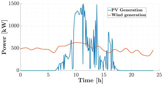
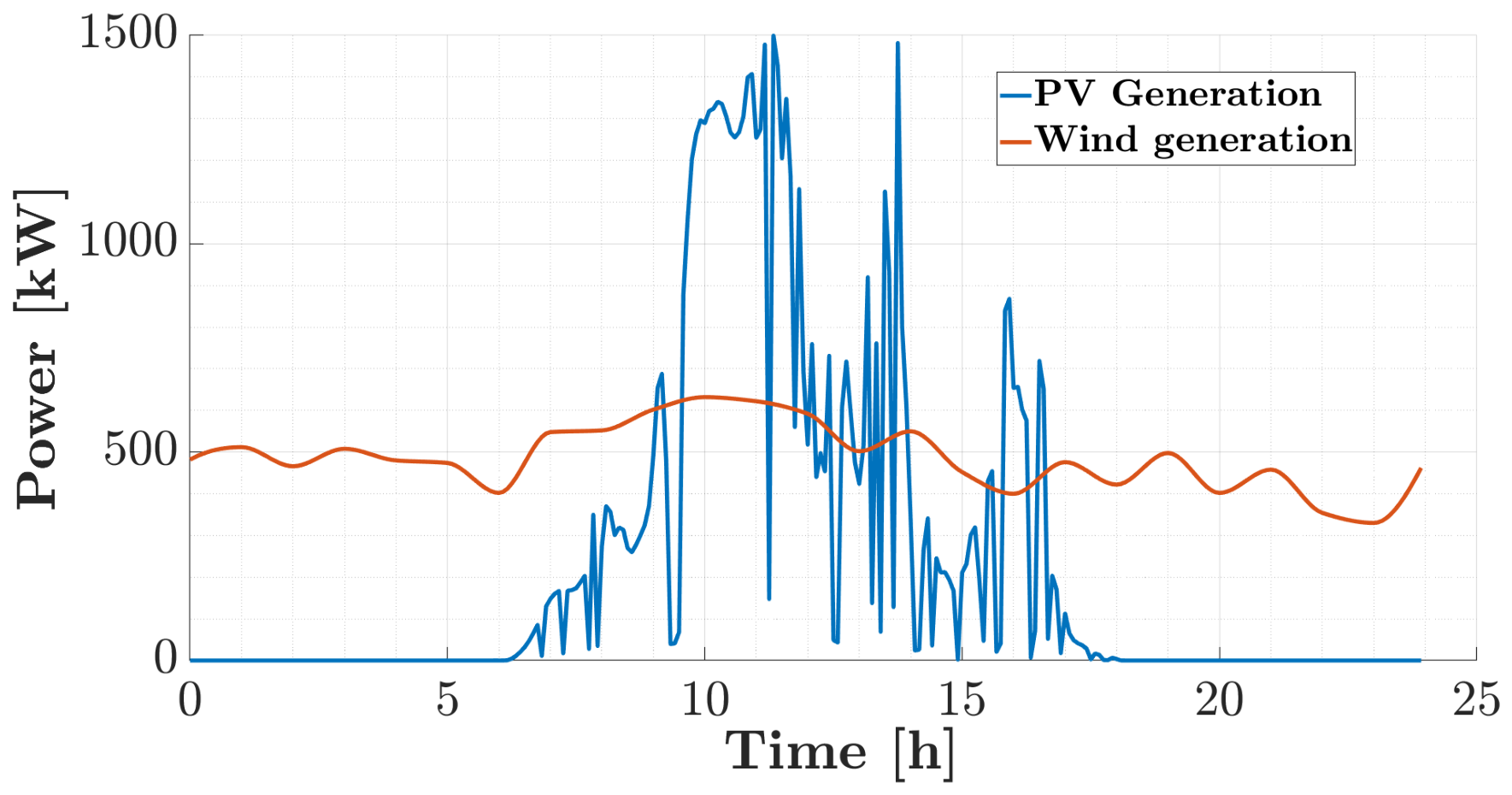
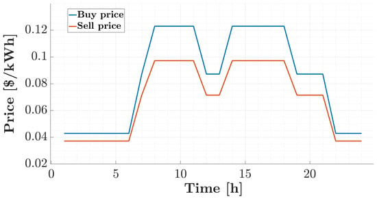
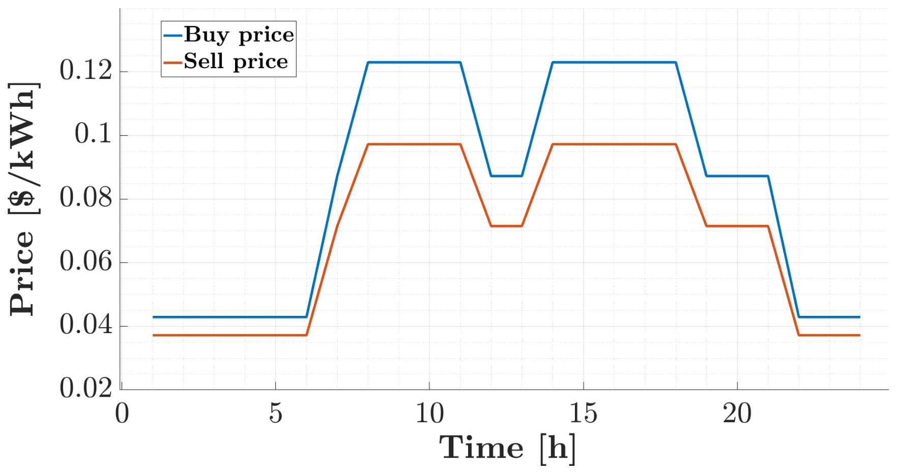
The operating costs of wind generation, photovoltaic generation, and the storage system were set at 0.075 $/kWh, 0.10 $/kWh, and 0.072 $/kWh, respectively. Figure 3 shows the hourly wind and photovoltaic generation profiles considered for the study day, while Figure 4 presents the electricity buy and sell prices in the market, which define the economic signals faced by the VPP [8].
Figure 3.
Generation profiles for photovoltaic (PV) and wind power on the study day.
Figure 4.
Dynamic electricity buy and sell market price tariffs ( and ) across the 24-h operational horizon.
The baseline environmental and economic profiles used for the evaluation scenario are depicted in Figure 3 and Figure 4. Figure 3 displays the daily power output profiles for the non-conventional renewable energy sources, where the photovoltaic (PV) generation reflects high intra-day solar variability with peak generation reaching approximately 1500 kW around noon, while the wind power output exhibits a relatively continuous profile oscillating around 400–600 kW throughout the 24-h horizon due to the AR(1) stochastic process. On the economic side, Figure 4 outlines the dynamic electricity market tariffs, illustrating a time-of-use pricing structure with peak prices occurring during morning and afternoon operational windows (0.125 $/kWh for buying and 0.098 $/kWh for selling), which directly incentivizes strategic battery cycling and demand-side response activation.
4.1. Active Demand Operational Scenarios
To represent distinct user flexibility profiles, four operational scenarios were defined for curtailable and shiftable loads, as detailed in Table 7. These scenarios simultaneously combine the user discomfort coefficient () and the maximum daily curtailment budget (), reflecting realistic demand response contract archetypes rather than an isolated single-parameter evaluation; a dedicated sensitivity analysis addressing individual parameter impacts is presented separately in Section 5.1. The operational scenarios were characterized as follows:
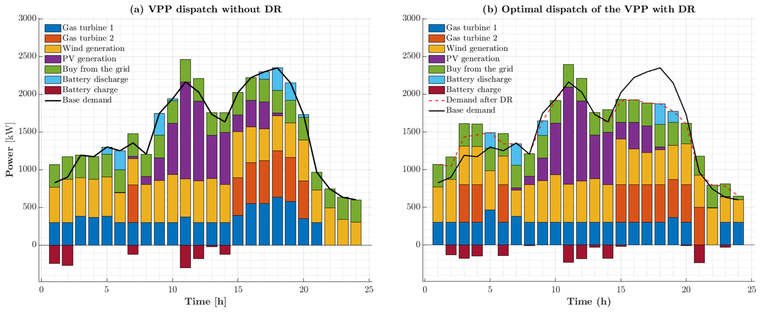
- Scenario 1 (Balanced): Assumes intermediate values for the discomfort coefficient alongside a conservative curtailment budget. This configuration allows moderate participation of curtailable loads without severely constraining flexibility. It serves as the benchmark case, with its dispatch results illustrated in Figure 5b.
- Scenario 2 (High Flexibility): Characterized by a low coefficient and an expanded reduction budget, resulting in minimal penalties for load curtailment. The daily demand-reduction capacity is high, rendering dispatch decisions predominantly driven by the economic incentive signal .
- Scenario 3 (Constrained Flexibility): Features an increased coefficient and a reduced daily curtailment allowance. Under this setup, the optimization model activates load curtailment exclusively during operational intervals where economic returns are most significant.
- Scenario 4 (Low Flexibility): Incorporates a high coefficient and a tightly restricted curtailment budget. This scenario models end-users who are highly sensitive to comfort disruptions, forcing the model to prioritize service continuity over economic savings.
Figure 5.
Optimal dispatch of the management model in VPP.
Table 7.
Parameter specifications for active demand operational scenarios.
Across all four scenarios, the benchmark electricity market price profile was held constant (Figure 4). This standard pricing background guarantees that all observed dispatch variations and cost dynamics are directly attributable to the specific combination of and .
4.2. Assumptions, Limitations, and Motivation of the Case Study Parameters
To clarify the scope of the results presented, Table 8 summarizes the main modeling assumptions and limitations of the proposed system.
Table 8.
Assumptions and limitations of the proposed model.
4.3. Computational Implementation
The optimization model was implemented in MATLAB R2018b, using the YALMIP modeling interface for the formulation of the MILP problem, which was solved with the commercial solver IBM ILOG CPLEX Optimization Studio 12.8. Simulations were executed on a system equipped with an AMD Ryzen 5 4600G processor and 16 GB of RAM. The computation times reported in Section 5 and Section 5.2 correspond to this hardware and software configuration.
5. Results
Figure 5 compares the optimal power dispatch of the VPP without Demand Response (Figure 5a) against the proposed DR strategy (Figure 5b) over a 24-h daily operational horizon, considering Scenario 1 from Table 7 as the baseline benchmark (, ). In both cases, the demand response scheme is solved jointly with unit commitment and generation dispatch within a single optimization formulation, activating DR exclusively when its operation yields a reduction in total system cost, thereby avoiding a decoupled pre-processing step.
In the case without DR, demand is primarily satisfied through conventional thermal gas turbine generation alongside available non-conventional renewable energy sources (NCRES). Incorporating battery energy storage system (BESS) dynamics allows the model to efficiently perform charge cycles during periods of excess renewable generation and discharge during peak consumption intervals (approximately 17–20 h).
Conversely, when the DR framework is activated, the optimization model leverages curtailable () and shiftable () load flexibility to reduce consumption during high-demand intervals and reschedule flexible processes to economically favorable hours. Table 9 summarizes the impact of this active demand strategy on the operational performance of the VPP. For the conservative curtailment budget evaluated in this baseline scenario ( daily), active DR dispatch decreases the total operational cost by , achieves a peak demand reduction of , and yields a Demand Peak Shaving Index (DPSI) of . These results confirm that, even under a restricted flexibility allowance, the proposed DR mechanism effectively mitigates peak load stress on the distribution grid during critical intervals, although aggregate economic savings remain modest under conservative parameters.
Table 9.
Economic dispatch results: VPP vs. VPP with DR.
Additionally, a slight increase of in emission costs is observed, rising from $11,170.74 to $11,367.02. This operational trade-off is explained by the load-shifting profile redistribution: to achieve peak shaving, flexible consumption is rescheduled into intervals where dispatchable thermal units operate at higher output levels to support the shifted load. This result underscores an important operational insight: while peak shaving provides crucial technical relief to the power grid infrastructure, it does not automatically yield proportional carbon reductions under tight curtailment budgets. A comprehensive evaluation of the joint economic and environmental benefits under expanded flexibility budgets is detailed in the sensitivity analysis in Section 5.1.
To complement the peak demand reduction metric, this study introduces DPSI, which quantifies the overall smoothing of the demand profile achieved through active demand response beyond the single absolute peak value. The DPSI is defined as the percentage reduction in the total hour-to-hour variation (total variation) of the demand profile:
where is the baseline demand profile and is the effective demand profile after DR activation (Equation (40)). While the peak demand reduction metric captures only the change in the single highest demand value, the DPSI captures the aggregate smoothing effect across the entire dispatch horizon, complementing peak-focused metrics with a measure of overall profile flatness relevant to network loading variability.
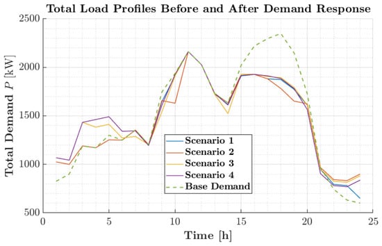
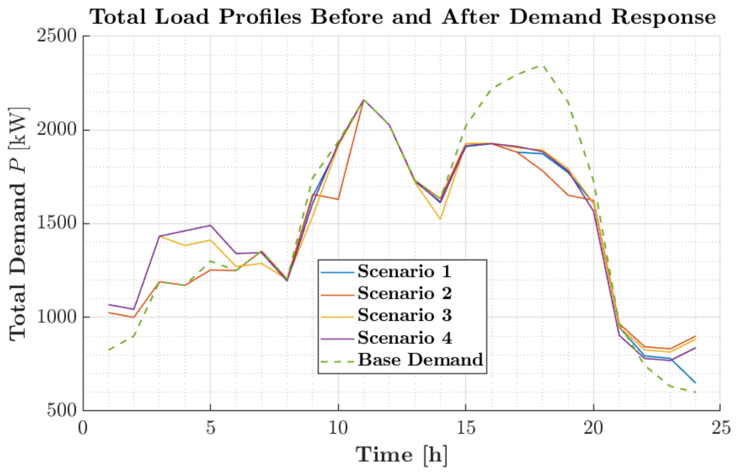
Figure 6 compares the baseline aggregated demand profile against the optimized load curves across the four operational scenarios. The most significant load modifications occur during peak consumption intervals (approximately hours 17–20), where implementing the DR strategy yields substantial peak shaving. A fraction of this energy is shifted toward off-peak hours, allowing the VPP to satisfy load requirements at lower operational costs by leveraging non-conventional renewable energy sources and battery storage cycling. Conversely, during mid-peak periods, the variation between the baseline and optimized demand profiles remains less pronounced.
Figure 6.
Baseline demand vs. demand after DR for each proposed scenario.
Scenarios characterized by lower discomfort coefficients (Scenarios 1 and 2) enable greater load profile reshaping, resulting in more significant peak demand reductions. In contrast, higher values (Scenarios 3 and 4) constrain demand-side flexibility, yielding load profiles that closely resemble the baseline demand. This flexible load response mitigates the reliance on conventional dispatchable thermal generation during peak hours, thereby decreasing both the overall operating costs and associated system emissions.
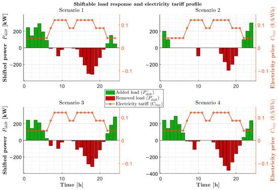
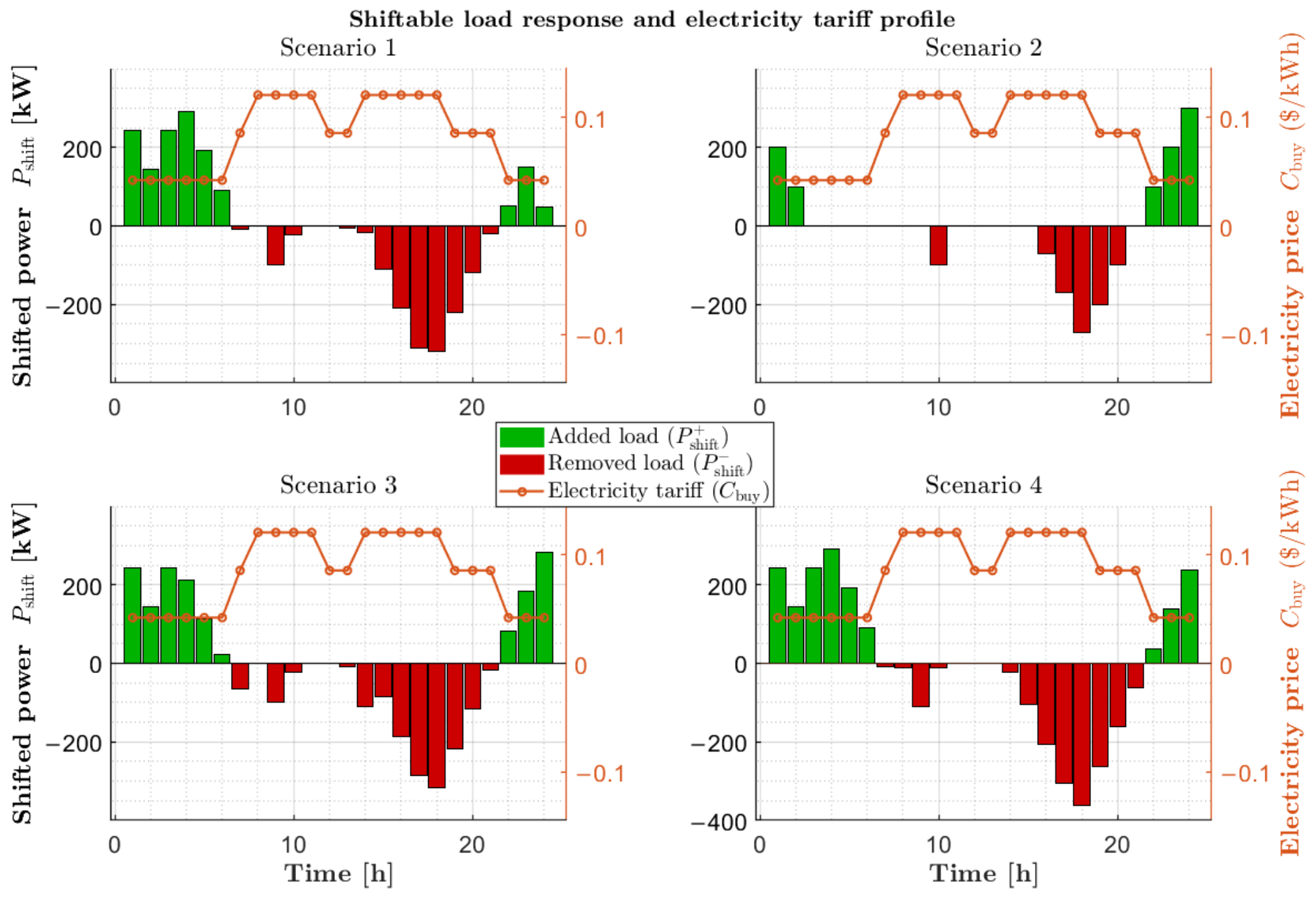
Figure 7 illustrates the operational response of shiftable loads across the four evaluated scenarios. The green and red bars represent the added (increased) and removed (decreased) load in each time interval, respectively, while the orange line indicates the market electricity buy price profile, which remains identical across all scenarios (Section 4.1).
Figure 7.
Behavior of shiftable loads in relation to the market electricity price.
The shiftable load profile is strongly governed by the market price signal: during periods of elevated electricity prices, the model curtails demand (red bars) and reschedules that energy toward low-cost intervals (green bars), concentrating the load displacement from peak hours (approximately 15–20 h) into the early morning off-peak hours where electricity rates are lowest. This temporal pattern remains consistent across all four scenarios because the shiftable load is modeled as an aggregated flexible resource whose power limits and ramp constraints (Table 7) do not vary with or . Consequently, the total magnitude of shifted energy remains equivalent across all cases, which aligns with the identical peak demand reduction reported in Table 10 ( for all scenarios). The inter-scenario variations discussed in Section 4.1 stem from the behavior of curtailable loads, whose activation directly depends on the specific coefficient and daily budget assigned to each case.
Table 10.
Results for the active demand scenarios.
A common pattern emerges across all scenarios: a fraction of the demand originally concentrated in peak hours is systematically shifted toward off-peak periods, strictly satisfying the energy conservation constraint for shiftable loads (Equation (40)). In this manner, the VPP manages demand in an economically efficient manner, consistently shaving peak power consumption across all evaluated operational settings (Figure 6), regardless of the discomfort penalty associated with curtailable loads.
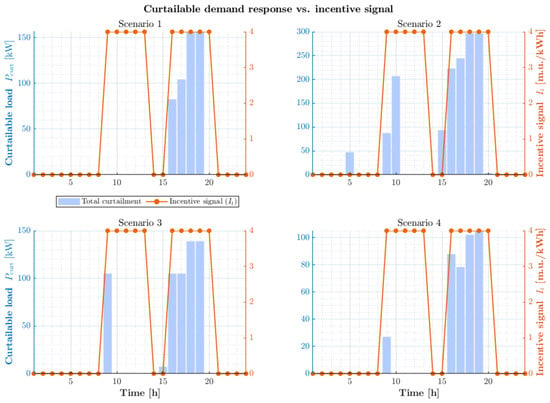
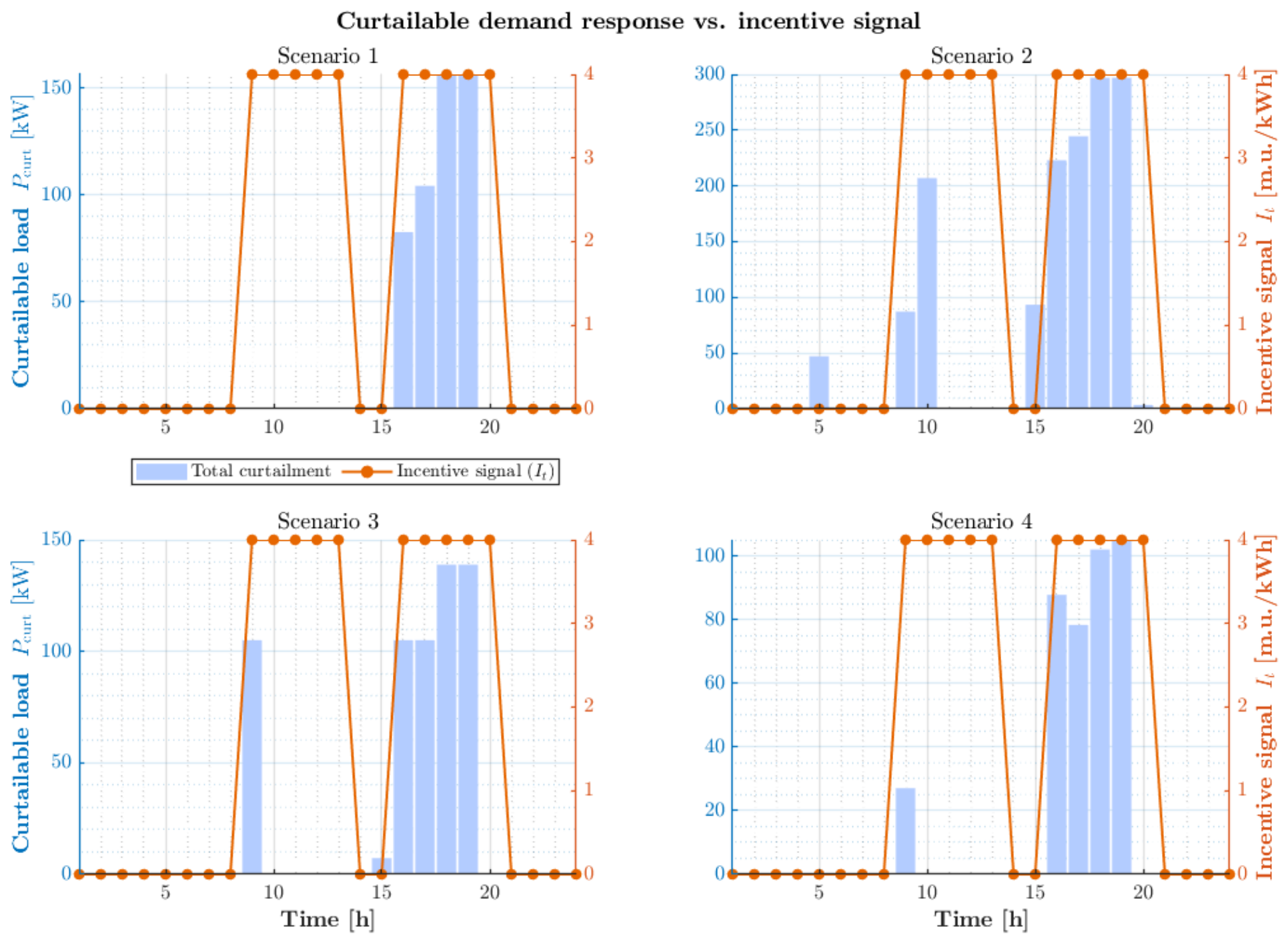
Figure 8 illustrates the relationship between the economic incentive signal and the aggregated demand reduction across the four evaluated scenarios. In each quadrant, the blue bars represent the total load curtailment , while the orange line denotes the incentive rate per unit of energy applied in each time interval (). Load curtailment concentrates almost exclusively during periods with non-zero incentives, confirming that the incentive-based DR scheme acts as the primary trigger for demand behavior adjustments.
Figure 8.
Behavior of curtailable loads in relation to the incentive agreed upon with the user and the comfort cost associated with the use of each curtailable load.
A comparison of the four operational settings revealed that, although the incentive signal profile remained similar, the magnitude and temporal distribution of varied significantly among the cases. These variations reflect the influence of the discomfort coefficient and daily curtailment allowance assigned to curtailable loads. In Scenario 2, for instance, the load curtailment response is highly concentrated around the peak demand hours. Conversely, in Scenarios 1, 3, and 4, the demand reduction was more conservative or spread across a broader set of operational intervals. Overall, Figure 8 demonstrates that active demand participation can be effectively modulated by tuning the incentive signals and discomfort coefficients (), achieving targeted peak shaving without excessively disturbing the baseline load profile during non-incentivized hours.
Table 10 summarizes the main performance metrics achieved by the VPP across the four evaluated operational scenarios, benchmarked against the base case without DR and holding the market price profile strictly constant (Figure 4). Across all scenarios, total operational cost reductions ranging from to are achieved relative to the non-DR baseline. Scenario 2 (lowest discomfort coefficient, expanded curtailment budget) yields the highest overall economic savings.
A notable result is that the peak demand reduction remains identical across all four scenarios at (shaving the absolute demand peak from to at 11:00 h). This uniformity occurs because peak shaving is predominantly driven by the aggregated shiftable load , whose power capacity and ramp limits (Table 5) remain constant across all cases. Conversely, parameters and , which vary between scenarios, govern curtailable loads exclusively. Consequently, the absolute peak demand reduction is determined by the temporal load-shifting mechanism, whereas the Demand Peak Shaving Index (DPSI) and aggregate economic benefits depend on the volume of additional curtailment activated under each specific parameter setting. This structural decoupling explains the observed DPSI variation ( to ) despite the constant peak demand reduction.
Scenario 2 achieved the greatest cost reduction () and emission penalty reduction (), consistent with its low discomfort penalty and expanded daily curtailment allowance, which enabled the optimizer to fully exploit high-incentive intervals without incurring severe discomfort penalties. In contrast, Scenarios 3 and 4, characterized by higher discomfort coefficients, exhibited a more conservative activation of curtailable loads. This behavior is reflected in higher emission costs ($10,709 and $11,077, respectively), despite achieving relatively high DPSI values, indicating that demand flattening in these cases relies primarily on temporal load shifting rather than net energy consumption curtailment.
Finally, across all evaluated cases, the execution time for each individual iteration consistently remained under 1 s (<1 s), which demonstrates full computational compatibility with day-ahead scheduling schemes and real-time MPC operation. Overall, the results show that the proposed strategy effectively enables the exploration of operational trade-offs involving generation costs, peak demand reduction, demand flexibility, and emission penalties, providing the VPP operator with a robust decision-making framework to tailor dispatch strategies according to specific economic and environmental priorities.
5.1. Sensitivity Analysis
The four operational scenarios defined in Section 4.1 simultaneously adjust the user discomfort coefficient and the daily curtailment budget , thereby modeling distinct demand flexibility archetypes. However, this joint variation prevents isolating the individual effect of each parameter on VPP operations. To address this limitation, three additional sensitivity experiments were conducted, wherein all other parameters were held constant while individually varying the discomfort coefficient, the daily curtailment budget, and the temporal price signal amplitude.
5.1.1. Sensitivity to the User Discomfort Coefficient
To evaluate the effect of the discomfort penalty associated with load curtailment, the daily budget was fixed at = 1500 kWh, and the discomfort coefficient vector from Scenario 1 was scaled using a common factor. The results are summarized in Table 11.
Table 11.
Sensitivity analysis to the user discomfort coefficient.
The results demonstrated a clear trend toward decreased load curtailment utilization as the discomfort coefficient increased. At low scaling factors, the available flexibility is heavily utilized; however, starting at a factor of 9, a sharp transition toward lower curtailment levels occurs. Specifically, between scaling factors 9 and 12, the utilized load curtailment drops from to , representing an approximate reduction.
The response was not strictly monotonic, as observed between factors 11 and 11.5. This non-monotonicity stems from the coupled nature of the optimization model, where adjustments to the discomfort penalty simultaneously alter the dispatch of thermal units, battery storage cycling, grid trading, and other active demand-side assets. Overall, the results indicate a high sensitivity of load curtailment to discomfort costs, exhibiting a pronounced threshold, beyond which curtailment activation drops rapidly.
5.1.2. Sensitivity to the Daily Curtailment Budget
The second experiment examines the influence of the maximum daily curtailment allowance. In this test, the discomfort coefficient vector was fixed at , while the daily budget was varied between and . The findings are presented in Table 12.
Table 12.
Sensitivity analysis to the daily curtailment budget.
For all the evaluated values, the utilized curtailment exactly equals the allocated budget limit. This indicates that, under the analyzed conditions, the constraint remains binding, confirming that sufficient economic value exists to exhaust the allowed curtailment allowance.
The total operating cost does not exhibit a strictly monotonic trend with respect to the budget limit owing to the multi-asset dispatch coupling. Nevertheless, the largest budget () yields the lowest overall operating cost (15,950.23 $), highlighting the economic benefit of enabling higher demand flexibility when system constraints permit.
5.1.3. Sensitivity to Price Signal Amplitude
Finally, the effect of electricity price spread on shiftable load behavior was evaluated. Keeping Scenario 2 parameters fixed ( and ), the temporal price spread was scaled using a factor f, defined as:
where is the mean buy price across the horizon, and f controls the price spread magnitude. Factor compresses peak-to-off-peak price differentials, whereas factor amplifies them. The results are presented in Table 13.
Table 13.
Sensitivity analysis to electricity price signal amplitude.
The results confirm that compressing temporal price spreads reduces shiftable load engagement. It eliminates price variations (, flat tariff) and drops shifted energy to zero, proving that load shifting responds strictly to price differentials rather than activating arbitrarily. However, introducing even a minor price spread () triggers of shifted energy, while factors reach saturation levels near maximum system capacity. In addition, with values between and , no significant additional load shifting or peak reduction occurs.
This behavior demonstrates a threshold-type response to price differentials: once a sufficient economic spread exists to offset shifting costs, the optimizer fully leverages the available load flexibility up to the physical operational limits.
In summary, the two active demand mechanisms exhibit distinct operational responses to economic signals. Shiftable loads exhibit a threshold-type sensitivity to temporal price spreads, rapidly reaching operational saturation once a minimum price spread is crossed. Conversely, curtailable loads show continuous sensitivity to discomfort penalty values, which heavily govern total curtailment activation. These findings complement the main scenarios and provide a clear picture of individual active demand parameters within the VPP framework.
5.2. Online Operation Under 5-Min Temporal Resolution
This section evaluates the operational performance of the VPP under a high-resolution 5-min simulation scale (288 daily intervals), contrasting the hourly resolution (24 intervals) analyzed in Section 5. Migrating to this fine-grained temporal resolution extends beyond simply refining the optimization time step; it strictly mandates scaling time-dependent parameters and physical constraints proportionally to the updated interval count. Specifically, this requires scaling the time step conversion factor embedded within the curtailment budget dynamics (Equation (42)) and the battery state-of-charge updating logic (Equation (35)), alongside the unit commitment ramp and operational bounds for conventional thermal generators (Section 3.3.1). Neglecting this explicit parameter scaling yields unphysical system behaviors and numerical inconsistencies, as discussed subsequently.
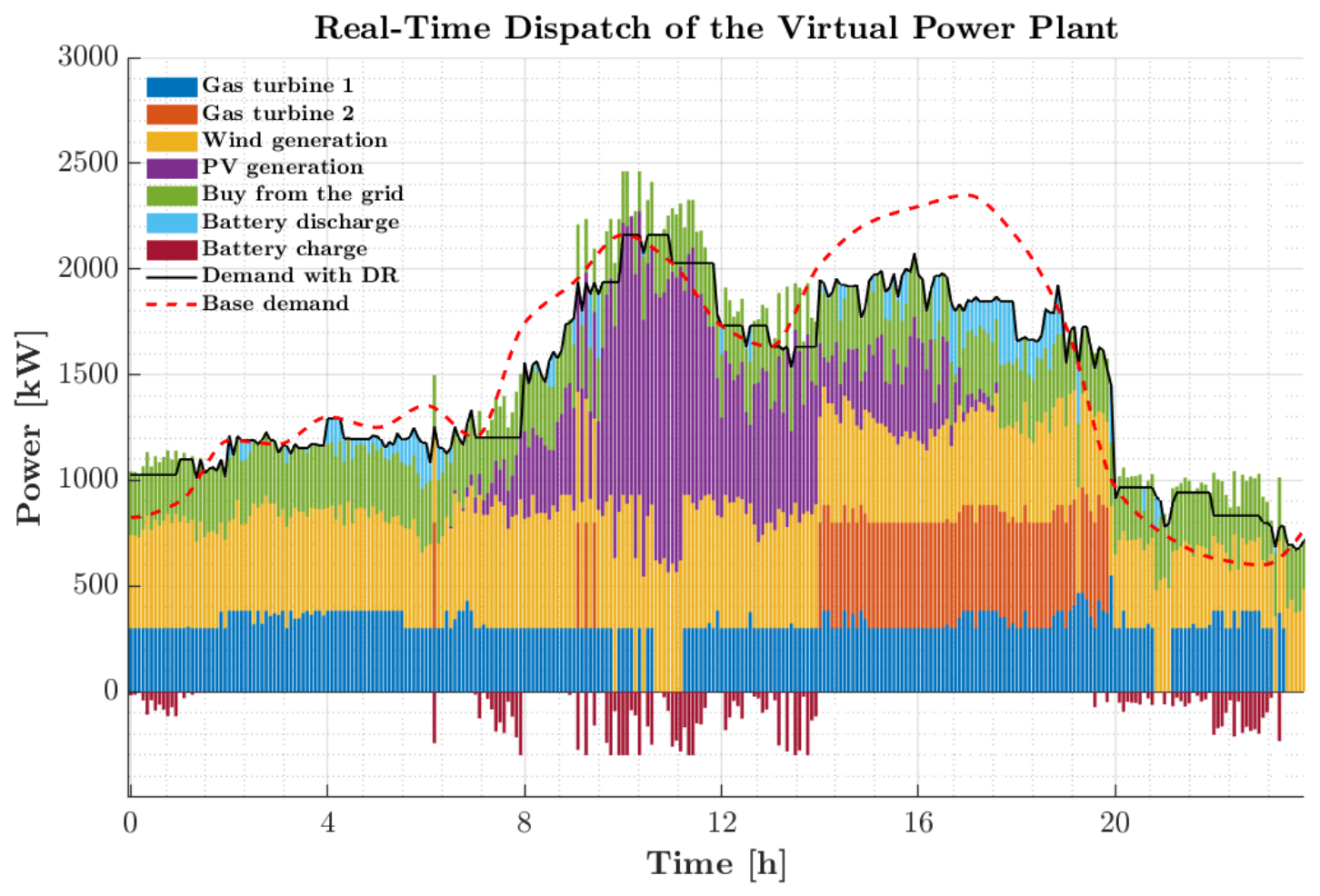
Figure 9 illustrates the VPP operational dispatch in this high-resolution online setting. The proposed dispatch scheme adequately covers the managed demand profile, whereas active demand response mechanisms effectively reduce consumption peaks and shift energy requirements toward intervals with lower operating costs. Comparing these outcomes with the hourly dispatch results from Section 4.1 demonstrates that the online receding horizon MPC framework manages short-term renewable generation variations with a higher temporal fidelity. This leads to more dynamic coordination of battery energy storage charge/discharge cycles and power exchanges with the main grid.
Figure 9.
VPP dispatch with real-time optimization.
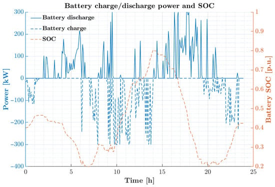
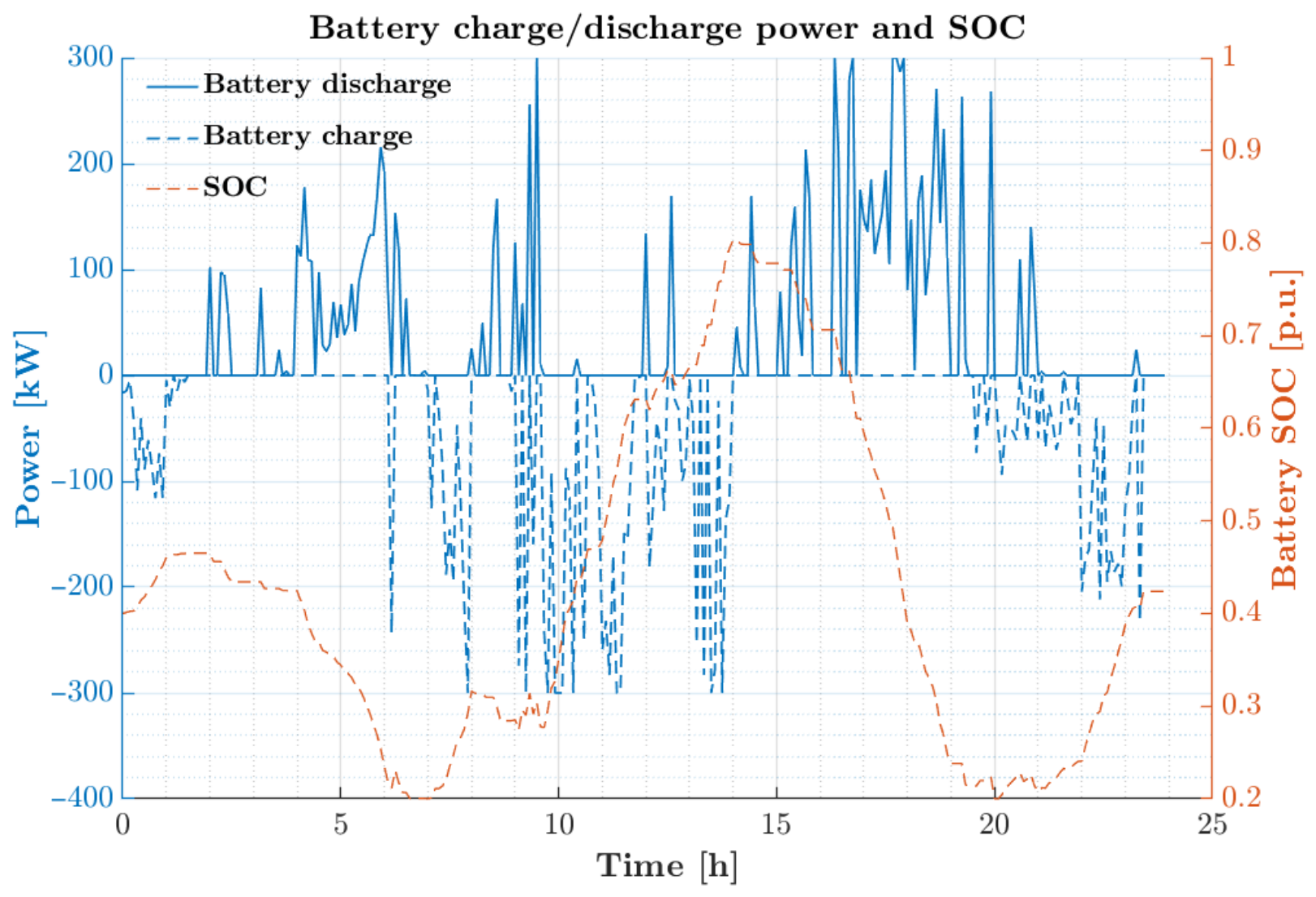
Figure 10 illustrates the battery charging and discharging cycles alongside the trajectory of its state of charge (SOC). The dashed curve depicts the SOC, which consistently remains within the prescribed operational limits while satisfying the terminal state constraint required to ensure operational continuity (Equation (37)). Although frequent, these cycling patterns are far from arbitrary; they directly respond to the proposed optimization strategy by charging predominantly during intervals of surplus renewable generation or low grid energy prices, and discharging during peak demand periods or high thermal generation cost intervals.
Figure 10.
Battery charging power, discharging power, and SoC.
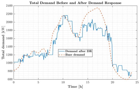
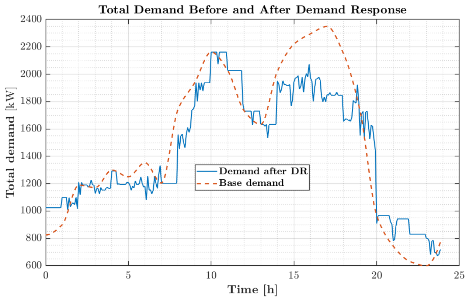
Figure 11 compares the baseline aggregated demand profile against the total demand managed under this high-resolution online setting. Under the proposed MILP-MPC scheme, the global peak demand was successfully reduced by compared to Scenario 2, while shifting the daily peak occurrence from 14:00 to 11:00. This demonstrates that the peak shaving capabilities are effectively preserved across high-resolution operational time scales. It should be noted that this reduction corresponds strictly to the net shift in the global maximum power peak. The overall combined effect of active demand management—encompassing both cumulative energy shifting and selective load curtailment—exceeds this percentage across the daily horizon, dynamically reshaping the profile to alleviate stress on the grid during critical high-cost intervals.
Figure 11.
Total demand before and after DR in real time (5 min).
When the DPSI metric is evaluated directly at the native 5-min resolution, a negative value is obtained, reflecting the high-frequency variability introduced by successive receding-horizon re-optimizations relative to the hourly baseline demand profile. After aggregating the 5-min results to hourly values, the DPSI increases to 19.05%. Although this value is lower than the 25.03 % obtained for the hourly Scenario 2 under the same daily curtailment budget of 1500 kWh, the 5-min formulation preserves a substantial demand-flattening effect while introducing additional short-term variability. The peak demand reduction remains 8.65%, consistent with the hourly evaluation. The daily curtailment budget of 1500 kWh was also respected.
Regarding total operational expenditure, an initial scaling inconsistency was identified within the thermal unit commitment constraints when migrating from 24 to 288 intervals. This mismatch induced excessive, unphysical start-up/shut-down cycling. After correcting the temporal scaling of the ramp and commitment-related constraints, the excessive cycling observed in the initial 5-min implementation was substantially reduced; nevertheless, explicit minimum up/down time constraints remain absent, and the total operating cost settled at $16,377, including $2240 in start-up/shut-down costs. Under the same 1500-kWh curtailment budget, this value is comparable to the hourly Scenario 2 benchmark of $16,013, with the difference attributed to the finer temporal resolution and receding horizon operation. This cost indicates that higher re-optimization frequencies enable more precise exploitation of generation, demand, and energy storage conditions throughout the day, provided that temporal model scaling is correctly enforced.
This implementation highlights the critical importance of rigorously verifying temporal constraint scaling and validation metrics when altering the MPC horizon resolution. Constraints or evaluation metrics calibrated for hourly steps do not automatically yield expected physical behaviors when applied unadjusted to 5-min intervals, a vital insight for expanding this model to alternative time steps in future work.
In terms of computational performance, the maximum execution time per MPC iteration was 1.69 s, occurring during the initial daily step where the prediction horizon spans its maximum length . In subsequent iterations, the effective horizon shrinks progressively toward the end of the day (Section 2.2), proportionately reducing solver execution times. This maximum execution time is fully compatible with online execution refreshed every 5 min, indicating that the optimization can be executed within the 5-min control interval under the tested computational conditions.
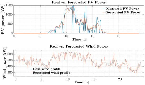
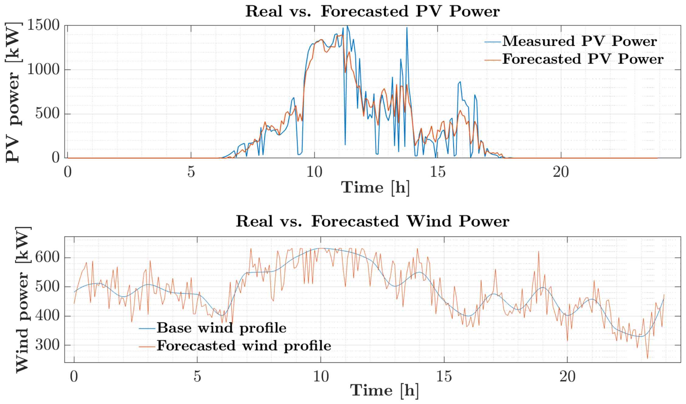
Figure 12 shows the measured photovoltaic power together with the forecast employed by the MPC, generated through a hybrid model that combines a physical irradiance-to-power conversion model (calibrated via least squares using historical measurements) with a machine learning model of the Gradient Boosting type LSBoost, trained to correct the residual between the physical estimate and the actual measurement (Section 2.4.1). On the validation set, this hybrid model achieves a 78.1% improvement in MAE compared to the standalone physical model at the 5-min resolution used in this simulation (Table 1). For the specific study day considered, the observed mean absolute error was 61.55 kW, lower than the validation average due to day-to-day climatic variability.
Figure 12.
Forecast generation profiles.
Regarding wind generation, because there are not enough historical data available to construct a dedicated forecasting model, the synthetic profile described in Section 2.4.2 is employed, which is generated through the AR(1) process defined by Equations (6) and (7).
6. Conclusions
This study developed an optimal active power management model for a virtual power plant (VPP) based on a MILP-MPC receding-horizon framework. The proposed approach coordinates dispatchable thermal generation, non-conventional renewable energy sources, battery energy storage, grid transactions, and active demand while considering operational constraints and economic signals. The results demonstrate the applicability of the proposed framework for coordinating heterogeneous VPP resources across different temporal resolutions.
The incorporation of active demand response reshaped the load profile and reduced the baseline peak demand by . However, the reduction in the peak at 14:00 h resulted in a new global maximum at 11:00 h, indicating that the available flexibility was insufficient to reduce demand uniformly throughout the day. The sensitivity analysis further showed that the daily curtailment budget was a binding constraint, whereas increasing the discomfort penalty reduced curtailable-load activation. The shiftable-load utilization was strongly influenced by temporal price differentials and approached saturation once sufficient economic incentives were available. These results highlight the importance of jointly considering the amount, timing, and economic conditions of demand flexibility.
The high-resolution 5-min simulations demonstrated the capability of the MPC formulation to update the system states and dispatch decisions at sub-hourly intervals. In addition, the hybrid photovoltaic forecasting model, combining a physical model with LSBoost, reduced the hourly MAE by up to relative to the standalone physical model. The multi-resolution analysis also showed that the temporal scaling of energy, flexibility, and commitment-related parameters is essential when changing the simulation time step. Inconsistent scaling can lead to unrealistic operational behavior, including excessive thermal unit start-up and shut-down cycling.
From an economic perspective, the coordinated management of generation, storage, grid exchanges, and active demand reduced operating costs under the evaluated scenarios while providing peak-demand mitigation. However, lower operating costs did not necessarily imply lower emissions, as the environmental outcome depended on the resulting loading of thermal generation and battery operation. This indicates that economic and environmental objectives should be explicitly coordinated when both are relevant to the VPP management strategy.
Future work will focus on incorporating explicit minimum up- and downtime constraints for thermal units, calibrating discomfort coefficients and incentive signals using empirical demand-response data, and extending the framework to electric vehicle fleets through vehicle-to-grid (V2G) operation. Further research will consider stochastic load forecasting and multi-day MPC simulations under variable electricity pricing conditions to evaluate the robustness of the proposed management strategy.
Author Contributions
Methodology, software, validation, formal analysis, investigation, resources, data curation, writing—original draft, writing—review and editing, visualization, B.B.-V., J.R.-F. and J.E.C.-B. Supervision, project administration, and funding acquisition, J.R.-F. and J.E.C.-B. All authors have read and agreed to the published version of the manuscript.
Funding
This work was supported by the project BPIN 2021000100499, funded by CTeI-SGR and Minciencias, Colombia.
Institutional Review Board Statement
Not applicable.
Informed Consent Statement
Not applicable.
Data Availability Statement
Data are contained within the article.
Acknowledgments
The work of Javier Revelo-Fuelagán was supported by the Universidad de Nariño. The work of John E. Candelo-Becerra was supported by the Universidad Nacional de Colombia Sede Medellín.
Conflicts of Interest
The authors declare no conflict of interest.
References
- International Energy Agency. Global Energy Review 2026; IEA: Paris, France, 2026; Available online: https://www.iea.org/reports/global-energy-review-2026 (accessed on 29 August 2026).
- Ministerio de Minas y Energía. Oportunidades y Desafíos Socioambientales de la Transición Energética Justa; Technical Report; Ministerio de Minas y Energía: Bogotá, Colombia, 2024. Available online: https://www.minenergia.gov.co/documents/13203/44._Desafios-TEJ-2024.pdf (accessed on 2 December 2024).
- Congreso de Colombia. Ley 1715 de 2014: Por Medio de la Cual se Regula la Integración de las Energías Renovables no Convencionales al Sistema Energético Nacional. Diario Oficial No. 49.150; 13 May 2014. Available online: https://www.funcionpublica.gov.co/eva/gestornormativo/norma.php?i=57353 (accessed on 2 December 2024).
- Naval, N.; Yusta, J.M. Virtual power plant models and electricity markets—A review. Renew. Sustain. Energy Rev. 2021, 149, 111393. [Google Scholar] [CrossRef] [Scilit]
- Rouzbahani, H.M.; Karimipour, H.; Lei, L. A review on virtual power plant for energy management. Sustain. Energy Technol. Assess. 2021, 47, 101370. [Google Scholar] [CrossRef] [Scilit]
- Blazek, V.; Vantuch, T.; Slanina, Z.; Vysocky, J.; Prokop, L.; Misak, S.; Piecha, M.; Walendziuk, W. A novel approach to utilization vehicle to grid technology in microgrid environment. Int. J. Electr. Power Energy Syst. 2024, 158, 109921. [Google Scholar] [CrossRef] [Scilit]
- Alhasnawi, B.N.; Sadeq, A.M.; Homod, R.Z.; Hussain, F.F.K.; Soběslav, V.; Bureš, V. An extensive examination of cyberattacks, cybersecurity, and energy management in smart grid, including new advancements and machine learning. Energy Convers. Manag. X 2026, 29, 101471, Correction in Energy Convers. Manag. X 2026, 29, 101535.. [Google Scholar] [CrossRef] [Scilit]
- Li, D.; Wang, M.; Shen, Y.; Li, F.; Lin, S.; Zhou, B. Low-carbon operation strategy of virtual power plant considering progressive demand response. Int. J. Electr. Power Energy Syst. 2024, 161, 110176. [Google Scholar] [CrossRef] [Scilit]
- Zhou, K.; Peng, N.; Yin, H.; Hu, R. Urban virtual power plant operation optimization with incentive-based demand response. Energy 2023, 282, 128700. [Google Scholar] [CrossRef] [Scilit]
- Yaghoubi, E.; Yaghoubi, E.; Maghami, M.R.; Rahebi, J.; Zareian Jahromi, M.; Ghadami, R.; Yusupov, Z. A Systematic Review and Meta-Analysis of Model Predictive Control in Microgrids: Moving Beyond Traditional Methods. Processes 2025, 13, 2197. [Google Scholar] [CrossRef] [Scilit]
- Brad Bustos Marambio, R.I. Control Predictivo para un Sistema de Coordinación de Micro-Redes Considerando Gestión de la Demanda. Master’s Thesis, Universidad de Chile, Santiago, Chile, 2022. [Google Scholar]
- Chang, W.; Yang, Q. Low carbon oriented collaborative energy management framework for multi-microgrid aggregated virtual power plant considering electricity trading. Appl. Energy 2023, 351, 121906. [Google Scholar] [CrossRef] [Scilit]
- Long, X.; Li, Y.; Li, Y.; Ge, L.; Gooi, H.B.; Chung, C. Collaborative Response of Data Center Coupled with Hydrogen Storage System for Renewable Energy Absorption. IEEE Trans. Sustain. Energy 2023, 15, 986–1000. [Google Scholar] [CrossRef] [Scilit]
- Li, Y.; Zhao, B.; Li, Y.; Long, C.; Li, S.; Dong, Z.; Shahidehpour, M. Safe-AutoSAC: AutoML-enhanced safe deep reinforcement learning for integrated energy system scheduling with multi-channel Informer forecasting and electric vehicle demand response. Appl. Energy 2025, 399, 126468. [Google Scholar] [CrossRef] [Scilit]
- Ruan, G.; Qiu, D.; Sivaranjani, S.; Awad, A.S.A.; Strbac, G. Data-driven energy management of virtual power plants: A review. Adv. Appl. Energy 2024, 14, 100170. [Google Scholar] [CrossRef] [Scilit]
- Huang, J.; Li, H.; Zhang, Z. Review of Virtual Power Plant Response Capability Assessment and Optimization Dispatch. Technologies 2025, 13, 216. [Google Scholar] [CrossRef] [Scilit]
- Zare, A.; Shafiyi, M.A. Virtual power plant models and market participation: A deep dive into optimization and real-world applications. Results Eng. 2025, 26, 105548. [Google Scholar] [CrossRef] [Scilit]
- Benavides-Vergara, B.; Revelo-Fuelagán, J.; Candelo-Becerra, J.E. Comparison Between MILP Optimization and Model-Based Predictive Control for Economic Dispatch with a Virtual Power Plant. In 2025 IEEE 7th Colombian Conference on Automatic Control (CCAC); IEEE: Piscataway, NJ, USA, 2025; pp. 1–6. [Google Scholar] [CrossRef] [Scilit]
- Dong, J.; Li, Y.; Lu, Y.; Han, S. Accuracy study of linearization methods for quadratic cost curves of thermal units in unit commitment problems. IET Gener. Transm. Distrib. 2022, 16, 2198–2207. [Google Scholar] [CrossRef] [Scilit]

Disclaimer/Publisher’s Note: The statements, opinions and data contained in all publications are solely those of the individual author(s) and contributor(s) and not of MDPI and/or the editor(s). MDPI and/or the editor(s) disclaim responsibility for any injury to people or property resulting from any ideas, methods, instructions or products referred to in the content. |
© 2026 by the authors. Published by MDPI on behalf of the International Institute of Knowledge Innovation and Invention. Licensee MDPI, Basel, Switzerland. This article is an open access article distributed under the terms and conditions of the Creative Commons Attribution (CC BY) license.