


Abstract
Deep visual recognition can turn ordinary video into interpretable motor knowledge, yet coordination among the joints of a single body during social interaction remains largely unexplored. We present an interactive playback visualizer that couples markerless pose estimation with the cross-wavelet transform to quantify amplitude co-modulation between all joint pairs. Amplitude co-modulation proved anatomically structured: bilateral homologous pairs exceeded cross-limb and head–body pairs even among pairs sharing no keypoint, where correlated tracking error cannot produce it. Within-limb pairs also scored high but share keypoints, so their elevation is confounded with measurement error and not treated as established. Co-modulation concentrated at low postural frequencies and showed no systematic temporal trend; each profile remained temporally consistent within the session, and equivalence to a flat trend was not established. Vocal activity correlated with upper-limb movement at gesture frequencies. Each participant’s 78-dimensional profile was individually distinctive: split-half identification reached 28.6% (95% CI 19.3–40.1%) against 1.4% chance, demonstrating within-session identifiability rather than a cross-session trait. No sex differences were detected in overall or category-level co-modulation, and equivalence was not established for any measure; women exceeded men in the micro-movement band, the narrowest and most attenuated by preprocessing, so that difference is reported but not interpreted.
1. Introduction
During face-to-face conversation, the human body produces a continuous stream of joint movements spanning the head, trunk, and all four limbs. These movements are not random: joints within the same limb flex and extend in coordinated sequences, gestural strokes co-occur with prosodic peaks, and postural shifts track the rhythm of turn-taking [1]. Decades of research on body movement in social interaction have focused almost entirely on the interpersonal level, asking whether two interlocutors become synchronized over the course of an exchange [2,3,4,5]. Comprehensive reviews have systematized the synchrony literature across disciplines [6,7], and dynamical systems approaches have formalized interlocutor coupling as the entrainment of nonlinear oscillators [8,9]. By contrast, the question of how joints within a single body coordinate with each other during conversation has received little systematic attention. The technical requirements for simultaneous, high-resolution tracking of multiple body segments have, until recently, confined such analyses to instrumented laboratory settings with wearable sensors or optical marker systems. Yet it is precisely this intra-body level that is most directly linked to the neural circuits that produce movement and most likely to be disrupted in conditions affecting motor control.
Motor control theory provides a principled framework for understanding why intra-body coordination should be structured. The classical degrees-of-freedom problem states that the nervous system must select, from an enormous space of kinematically possible trajectories, those that accomplish a task with economy and precision. One solution is the formation of coordinative structures, temporary functional linkages among joints that reduce the effective dimensionality of the motor command [10,11]. Latash [12] formalized this idea within the synergy concept, showing that the motor system actively exploits redundancy by co-varying joint angles along manifolds that leave task-relevant variables invariant, a principle that was subsequently quantified by the uncontrolled manifold framework [13].
At the muscle level, d’Avella and colleagues [14] demonstrated that natural movements in vertebrates can be decomposed into a small set of muscle synergies, suggesting that the spinal cord stores a modular repertoire of motor primitives that can be flexibly combined. Optimal feedback control theory further predicts that the nervous system minimizes task-relevant variability while allowing task-irrelevant variability to accumulate [15], a principle that naturally produces correlated fluctuations among joints sharing a biomechanical chain. At the spinal level, central pattern generators (CPGs) organize rhythmic alternation within and between limbs through reciprocal inhibition and propriospinal coupling [16,17], producing the characteristic patterns of interlimb coordination observed during locomotion [18]. Whether analogous modular structures govern body coordination during the physically unconstrained, cognitively demanding context of conversation, and whether their disruption could serve as a clinical marker, remain open questions.
The clinical motivation is substantial. In Parkinson’s disease, progressive degeneration of basal ganglia circuits disrupts the amplitude and timing of coordinative structures, manifesting as bradykinesia, rigidity, and impaired bilateral coordination of gait [19,20]. Current assessment relies on categorical rating scales that provide limited sensitivity to early-stage motor changes. Quantitative gait analysis has demonstrated that bilateral coordination measures can detect Parkinsonian asymmetry before clinical onset [19], but these measures require instrumented walkways or wearable inertial sensors. In autism spectrum disorder, motor coordination difficulties are well documented and may emerge before core social-communicative features [21,22]. Torres and colleagues [23] proposed that micro-movements carry a motor signature that distinguishes autistic from neurotypical individuals, and Anzulewicz et al. [24] showed that gesture kinematics during tablet gameplay could identify autistic children with high sensitivity. The broader field of digital phenotyping has highlighted the potential of passively collected behavioral data to provide continuous, ecologically valid biomarkers [25,26], but progress has been limited by the lack of methods to noninvasively capture whole-body coordination in naturalistic settings.
Recent advances in deep learning-based computer vision have made it feasible to address this gap. Convolutional neural network architectures trained on large-scale annotated datasets can now estimate two-dimensional pose from monocular RGB video with accuracy approaching manual annotation [27,28]. Frameworks such as DeepLabCut [27] and OpenPose [29] use deep residual network backbones to extract hierarchical visual features from each video frame, producing spatial likelihood maps for each anatomical keypoint. Complementary tools, such as Social LEAP Estimates Animal Poses (SLEAP) [30], have extended multi-animal tracking across diverse species. The introduction of pretrained foundation models, including the SuperAnimal family [31], has eliminated the need for user-collected training data, enabling zero-shot pose estimation on novel recording setups through transfer learning [31,32]. These frameworks have already been validated for gait analysis [33] and for quantifying gesture–speech synchronization [34], demonstrating utility beyond their original training domain. Combined with time–frequency signal analysis [35,36,37], this deep learning approach enables characterization of the full pairwise co-modulation structure of the body across temporal scales.
A critical advantage of the wavelet-based analytical framework is that it places signals of different origin on a common time–frequency grid. Because the continuous wavelet transform produces a time–frequency representation with explicit temporal indexing, kinematic signals extracted from video can be compared, coefficient by coefficient, with any concurrently recorded physiological signal that admits the same decomposition. For instance, sound, electroencephalography (EEG), electromyography (EMG), electrocardiography (ECG), respiration, and skin conductance. The cross-wavelet transform can then quantify coupling between brain, muscle, cardiac, or respiratory activity and specific joint movements at each frequency and time point, without requiring temporal averaging or trial-based designs. This transforms a single video camera into a continuous source of kinematic features that can be integrated with the full spectrum of physiological measurements. The present study demonstrates this pipeline across the kinematic domains of body movements, voice, and intra-body coordination.
A parallel development motivates the study from an individual-differences perspective. Functional neuroimaging has demonstrated that each person’s pattern of cortico-cortical connectivity is sufficiently idiosyncratic to serve as a connectome fingerprint, permitting identification across scanning sessions [38]. If the body’s coordination structure during conversation reflects stable properties of the individual motor system rather than transient social states, then the pattern of which joints co-modulate most strongly could support analogous identification from a simple video recording. Identification within a single recording and identification across separate recordings are different claims, and only the first is addressed here. Gait studies have provided initial evidence. Walking patterns captured through deep learning pose estimation are individually recognizable [33,39], but no comparable demonstration exists for whole-body coordination during seated social interaction.
The intersection of deep learning, signal processing, and behavioral neuroscience creates a natural fit with the aims of knowledge extraction research. Pose estimation provides the raw kinematic features; wavelet decomposition transforms those features into a multi-scale time–frequency representation; and the resulting co-modulation matrices constitute a structured, interpretable form of knowledge about the individual’s motor organization. Each stage, from keypoint detection through feature engineering to individual identification, represents a concrete application of machine learning for extracting clinically relevant behavioral knowledge from unstructured video data. The present study applies this pipeline to characterize intra-body joint coordination across 70 individuals during naturalistic face-to-face conversation. Six questions are addressed: (1) whether amplitude co-modulation follows anatomical boundaries, (2) how it distributes across frequency bands, (3) whether it remains stable over the course of the conversation, (4) how it relates to vocal activity, (5) whether the resulting coordination profile is sufficiently individual-specific to identify participants within a session, and (6) whether this coordination architecture differs between women and men.
2. Materials and Methods
2.1. Participants and Ethical Considerations
Seventy healthy young adult individuals (N = 70; 47 women, 23 men) participated in 15 min spontaneous face-to-face conversations recorded in a controlled indoor setting. Each of the 70 participants engaged in a separate conversation with their own conversational partner, who was not part of the analyzed sample and whose kinematic data were not included in the dataset. Because each participant’s partner was unique to that session, no two of the 70 participants shared a conversation or an interlocutor, ensuring full statistical independence across the sample. All participants provided written informed consent prior to participation, and the study protocol was approved by an institutional ethics committee of Benemérita Universidad Autónoma de Puebla (Protocol number VIEP/2702/2026). Procedures conformed to the Declaration of Helsinki. No participant reported neurological or musculoskeletal conditions that could affect movement. Participants were young adults recruited from the university community, aged 20 to 35 years (mean 25.6, SD 3.3). All participants were right-handed, and the seating arrangement was identical in every session. The conversational partners were acquaintances who accompanied each participant; their pose was tracked only to separate identities and their kinematics were never analyzed, so their demographic characteristics do not enter any reported statistic. The target participant in each recording was designated before recording began and before any data inspection.
2.2. Recording Protocol
Each participant was seated facing their accompanying conversational partner at a distance of 250 cm in a controlled indoor room with standardized overhead lighting. Participants engaged in 15 min of spontaneous conversation. The same open-ended prompt was given in every session: which scientific invention they considered to have most transformed everyday life. No scripted tasks, forced turn-taking, or movement instructions were imposed. A single frontal RGB camera (Steren, Model COM-126, Mexico) (1920 × 1080 pixels, 60 fps) recorded both individuals within one frame, and only the designated participant’s data were retained for analysis. Video was captured and written to disk with OBS Studio (OBS Project; https://obsproject.com, accessed on 21 August 2026). The 250 cm separation between participants, with the camera positioned frontally beyond them, follows from the single-camera design. It is the distance at which both seated individuals fall entirely within one 1920 × 1080 frame at full resolution, which is what allows every keypoint of both people to be tracked with one consumer device and no instrumentation of the participants, and it keeps each person unoccluded by the other for the whole session. The trade-off is that this spacing is wider than an intimate conversational distance and may reduce the rate of gesture and mutual gaze, a consideration that bears on the voice–body results in particular. A microphone captured the audio signal at 44.1 kHz.
2.3. Deep-Learning-Based Body Pose Estimation with DeepLabCut
Body pose was estimated frame-by-frame using DeepLabCut version 3.0.0rc12 (https://contrib.deeplabcut.org/) [27], an open-source deep learning framework for markerless pose estimation. Pose was estimated with the RTMPose-x backbone distributed with the SuperAnimal-HumanBody model. Early layers capture edges and textures, intermediate layers encode body-part shapes, and deep layers represent spatial relationships among anatomical landmarks. Rather than decoding a spatial heatmap, RTMPose treats localization as a classification over horizontal and vertical coordinate bins, which is what allows it to run at this resolution on a single consumer GPU.
Rather than training the network from scratch on manually annotated frames, the study used the SuperAnimal-HumanBody pretrained model [28,31]. SuperAnimal models are foundation models for pose estimation trained on large-scale, multi-species annotated datasets using a semi-supervised learning strategy. A teacher model generates pseudo-labels on unlabeled frames, and a student model is trained on the combined real and pseudo-labeled data, with iterative refinement across training rounds [31]. This produces models that generalize across species and recording conditions without requiring any user-provided training data, a zero-shot transfer learning paradigm that eliminates the manual annotation bottleneck traditionally limiting scalability [32].
The SuperAnimal-HumanBody model operates in a two-stage architecture. In the first stage, a Faster R-CNN object detector with a MobileNetV3-Large-FPN backbone scans each video frame and proposes bounding boxes around each detected person. The Feature Pyramid Network constructs feature maps at different spatial resolutions, enabling detection regardless of apparent size. In the second stage, each detected bounding box is cropped and passed through the pose estimation backbone (RTMPose-x), which estimates 17 anatomical keypoints per individual: nose, left and right eye, left and right ear, left and right shoulder, left and right elbow, left and right wrist, left and right hip, left and right knee, and left and right ankle. Each keypoint prediction is accompanied by a confidence score. This score is the peak response of the coordinate classifier and is not normalized to a probability: higher values mean greater confidence, and in the present recordings about one value in six lies between 1.0 and 1.4.
Inference was performed using the DeepLabCut function video_inference_superanimal() with the following parameters: model_name = “resnet_50”, detector_name = “fasterrcnn_resnet50_fpn_v2”, pcutoff = 0.4, video_adapt = True, and batch sizes of 1 for the detector, the pose estimator, and the adaptation step. DeepLabCut resolved these to the weights distributed with superanimal_humanbody, and the model actually applied was RTMPose-x with a Faster R-CNN MobileNetV3-Large-FPN detector, which is the identifier recorded in the scorer field of every output file (superanimal_humanbody_rtmpose_x_fasterrcnn_mobilenet_v3_large_fpn). The same likelihood threshold is applied during signal conditioning (Section 2.5). The video_adapt option enables test-time domain adaptation, in which the pretrained model is briefly fine-tuned on pseudo-labels generated from the target video itself, improving accuracy on recording conditions that differ from the training distribution. This adaptation is automatic and requires no user intervention.
To accommodate GPU memory constraints imposed by 15 min recordings at 60 fps (approximately 54,000 frames per session), each video was segmented into 60 s clips using FFmpeg 7.1 prior to inference. Keypoint coordinate files (.h5 format) from successive clips were concatenated into a single continuous time series for each video, with frame indices adjusted using a cumulative offset to maintain temporal continuity. Batch size was set to 1 for both the detector and the pose estimator. All inference ran on an NVIDIA GeForce GTX 1660 Ti (6 GB) (NVIDIA Corporation, Santa Clara, CA, USA) under Windows 11 Pro (Microsoft Corporation, Redmond, WA, USA) with Python 3.10, at approximately 12 min of processing per minute of 60 fps video. Video adaptation was applied per 60 s clip rather than per session, so each clip was fine-tuned on its own pseudo-labels. Segmentation used stream copy without re-encoding, so frames are bit-identical to the source, and the per-clip coordinate files were concatenated with a cumulative frame offset that preserves a continuous, gap-free index.
We quantified the resulting boundary effect directly. Across the 70 participants, comparing the 12,721 angle-by-frame transitions that fall on a clip boundary against the 45.8 million that do not, the mean absolute angular step was 1.03 degrees at boundaries and 0.69 degrees elsewhere, a ratio of 1.51. The pooled effect size is negligible (Cohen’s d = 0.15) and the two distributions overlap almost entirely: the median boundary step sits at the 62nd percentile of ordinary variation, and 9.4% of boundary steps exceed the 95th percentile of that variation against the 5% expected by chance. A paired test on subject means is significant (d = 0.77), so the shift is consistent across participants, but its magnitude is 0.35 degrees per frame and it applies to 14 of the 50,400 frames in a recording, or 0.028%. Since every reported quantity is averaged over multi-second windows, a sub-degree perturbation at 0.028% of frames cannot account for the reported structure.
A periodic boundary artefact would also deposit power at 1/60 Hz and its harmonics, and we tested for this directly. Across the 70 participants, the power at the first thirty harmonics relative to the neighboring non-harmonic frequencies gave a median ratio of 0.983 (IQR 0.971–0.993); only 15.7% of sessions exceeded unity, and the largest ratio was 1.020. The harmonics therefore do not stand out above the surrounding background, and the postural band shows no periodic signature of the clip structure. Future implementations should nonetheless adapt per session.
2.4. Subject Identification and Identity Correction
Because both the participant and their conversational partner appear in the same frame, DeepLabCut processes each frame independently in multi-animal mode, and the identity labels assigned to detected individuals can swap between frames, a problem known as identity switching. A position-based assignment algorithm was implemented. The horizontal (x) coordinate of each detection’s torso centroid (mean of nose, left and right shoulder, and left and right hip) was computed frame-by-frame. A 2-means clustering on all valid torso x-values identified the stable spatial home position of the left-seated and right-seated individual. In each frame, the complete set of 17 keypoints from the detection, along with the torso centroid closest to each home position, was assigned to the corresponding individual. Only the keypoints assigned to the designated participant were retained for subsequent analysis; the partner’s pose was tracked solely to enable reliable identity separation.
A quality-control step rejected keypoint coordinates exhibiting physically impossible jumps between consecutive frames. The body scale was estimated as the median shoulder-to-hip distance across the session. Any frame-to-frame displacement exceeding 60% of this body scale within a single 1/60 s interval was flagged as a tracking artifact and set to NaN. Keypoints with detection likelihood below 0.4 were also set to NaN. Frames containing fewer than two detected individuals were excluded. The 60% threshold was chosen to exclude displacements that no seated conversational movement can produce within 17 ms, while retaining large but plausible gestures. With a body scale of 143.5 ± 18.2 px the threshold corresponds to roughly 86 px, and it flagged 0.02% ± 0.07% of frames. Combined with likelihood filtering and sentinel removal, the full quality-control pipeline flagged 0.59% ± 0.99% of frames (median 0.17%). An interactive HTML-based viewer built with Plotly version 6.5.2 and JavaScript (ECMAScript 2017/ES8) enabled frame-by-frame visual inspection with keypoint overlay. No systematic manual correction was applied to the analyzed dataset, so the pipeline is fully automated in the sense that no manual annotation enters the kinematic time series.
Pose Estimation Quality Metrics
Across the 70 participants the proportion of missing keypoint coordinates, defined as frames where a keypoint fell below the likelihood threshold or was rejected by quality control, was 0.137% on average. The head/neck angle carried the highest rate, consistent with an ear becoming occluded during the head rotation that this angle is meant to measure, which we note as a constraint on the interpretation of that row. The identity-assignment swap rate, defined as the proportion of frames in which the target participant’s torso centroid fell closer to the partner’s spatial cluster than to their own home position, averaged 22.5% ± 15.7% (median 22.1%, range 0.1–49.2%). This quantity indexes how often the two seated individuals approached each other, not how often the tracker failed: assignment is recomputed from torso proximity in every frame, so a high rate does not by itself compromise identity. Frames excluded for having fewer than two detections retained their timestamps, so no temporal compression was introduced.
Localization accuracy was assessed against manual annotation, the reference standard used to benchmark the SuperAnimal models themselves [31]. A stratified sample of 50 frames was annotated by hand and compared with the network output over 831 keypoint instances. The global root-mean-square error was 12.19 px, or 8.5% of the median shoulder-to-hip body scale, with a median error of 7.67 px. The proportion of correct keypoints was 63.8% within 10 px, 78.6% within 15 px and 95.1% within 25 px.
Accuracy was strongly regional, and the pattern matters for how the results should be read. Head keypoints were localized almost exactly (RMSE 4.57 px, 99.2% within 10 px). Upper-limb keypoints were intermediate (RMSE 10.25 px, 64.8% within 10 px). Lower-limb keypoints were the least accurate (RMSE 17.42 px, 32.4% within 10 px), with the hips worst of all (right hip RMSE 24.16 px). This is the expected consequence of seated frontal recording, in which the hips are occluded by the torso and the chair, and it means that the lower-limb entries of the co-modulation matrix rest on noisier coordinates than the upper-limb entries. The lower-limb and head–body categories are also those with the smallest excess over the surrogate null (Section 3.6).
2.5. Joint Angle Computation, Signal Conditioning, and Normalization
Following standard practice in markerless pose-estimation kinematics in DeepLabCut [27] each joint angle was computed from a kinematic chain of three keypoints: a central vertex and its two anatomical neighbors.
Given the three keypoints for each angle, the vertex V and its two neighbors P1 and P2 (each a position vector of image-plane coordinates), the two vectors forming the angle are defined as differences from the vertex. Taking both as differences from V makes the angle invariant to translation: it depends on the configuration of the three keypoints and not on where the participant sits in the frame. The two vectors are
The angle at the vertex is then
Because both a and b vectors originate at V, the vertex position cancels out, yielding the translation invariance stated above. The angle depends only on local body geometry, not on the subject’s absolute position in the frame.
In every case, P1 and P2 are the two keypoints that form the angle at the vertex, as listed in Table 1; they are not necessarily three consecutive joints along a limb, since several angles (for example, the shoulder and distal arm angles) draw one neighbor from across the trunk or from a more proximal segment.
Table 1.
Keypoint triplets defining each of the 13 joint angles. Each angle is measured at a vertex keypoint, with P1 and P2 the two neighboring keypoints whose vectors from the vertex form the angle. Twelve angles correspond to the six bilateral joints (shoulder, elbow, distal arm, hip, knee, and distal leg) computed separately on the left and right sides; the thirteenth captures lateral head rotation, measured at the nose between the two ears. The Measurement column names the anatomical motion each angle captures. All angles are computed in the camera image plane and take values in [0°, 180°].
The first and last 30 s of each recording were discarded, yielding approximately 14 min of data analyzed. Three conditioning steps were applied sequentially. (1) NaN gaps of 30 frames or fewer (0.5 s at 60 fps) were filled by linear interpolation; longer gaps and edge NaNs were filled by forward-fill. Across the 70 participant records, 0.368% of keypoint coordinates fell below the likelihood threshold, distributed over 38,776 gaps whose median length was 2 frames (90th percentile 12, 99th percentile 70, maximum 848). Because 96.8% of gaps were 30 frames or shorter and therefore interpolated, forward-fill applied to 0.139% of all coordinates, which bounds the flat plateaus it can introduce. (2) A running median filter with a 5-frame window (~83 ms) removed isolated spikes caused by residual tracker noise. (3) Each time series was min-max normalized per session to [0, 100]%. This removes absolute range-of-motion differences between individuals and preserves the shape of the temporal fluctuations, but the scaling depends on the session minimum and maximum and is therefore sensitive to isolated extreme values. Because the normalization discards amplitude, all reported quantities describe relative co-modulation structure and not absolute movement magnitude.
We repeated the full category analysis under three alternative scalings to establish which conclusions depend on this choice. With raw degrees, with robust scaling by the median and interquartile range, and with z-scoring, the categorical structure remained highly significant (Friedman p = 8.4 × 10⁻³⁵, 1.6 × 10⁻²³ and 3.5 × 10⁻²³ respectively, against 2.7 × 10⁻²⁸ for min-max). The ordering of the two highest categories was not stable: intra-limb leads under min-max and z-scoring while homologous leads under raw degrees and robust scaling, which is consistent with the two not differing significantly from each other. Under z-scoring, head–body rose above cross-limb, reversing the bottom of the ordering. Agreement at the level of individual pairs was moderate (Spearman ρ against min-max of 0.59, 0.17 and 0.22). The categorical result is therefore robust to the scaling choice, whereas the ranking of individual pairs is not, so the conclusions below are drawn at the category level.
2.6. Continuous Wavelet Transform
The continuous wavelet transform (CWT) decomposes a time series into a time–frequency representation, providing instantaneous power at each time–frequency point. The Morlet mother wavelet with central frequency ω0 = 6 was used, following established recommendations [35,37]. Two separate decompositions were computed, each with its own sampling rate and its own set of scales. For single-session visualization of a joint-angle pair (Figure 1d) the CWT was computed on the native 60 fps signal over 48 logarithmically spaced scales spanning 0.0159 to 28.65 Hz, entirely below the 30 Hz Nyquist frequency of that signal. For every population-level matrix and every statistic reported here, joint angle series were first block-averaged over non-overlapping 4-frame windows to an effective rate of 15 Hz (dt = 4/60 s) and the scales were recomputed accordingly, spanning 0.0159 to 7.162 Hz and therefore remaining below the 7.5 Hz Nyquist frequency of the decimated signal. No analysis was performed above the Nyquist limit of its own signal. The implementation uses the Morlet formulation of Torrence and Compo [35] with scale-to-frequency conversion f = ω0/(2πs) for ω0 = 6, and signals were zero-padded to the next power of two to limit edge effects. The cone of influence (COI) is set by the e-folding time of the wavelet, τs = √2 s expressed in units of the sampling interval; points closer to either edge of the record than τs are those the transform cannot resolve without edge contamination. The COI covers most of the record at the frequencies that carry the reported power, and its effect is confined to the slowest scales, where the covered fraction falls to about 80% at 0.016 Hz; per-scale fractions are given in Table S2. The COI is computed for every transform and is shown as shading in the single-session displays. Session averages are taken over the full time–frequency plane rather than over the COI alone, and Section 3.6 reports what changes when the average is restricted to the cone.
Figure 1.
Continuous wavelet decomposition of intra-body coordination in a representative individual during spontaneous conversation. (a) Body pose estimated from a single video frame. Colored circles indicate the 17 tracked keypoints; gray lines connect anatomically adjacent landmarks. The 13 joint angles are overlaid and numbered 1–13 as in Table 1: each arc spans the measured angle at its vertex keypoint, and the two dashed arrows mark the vectors that define it. (b) Raw joint angle time series (degrees, 0–180) for four representative joints across the full 14 min session (after 30 s trim from each end). Slow oscillations (<0.5 Hz) reflect postural sway; rapid transients correspond to gestural activity. (c) The same series after conditioning and min-max normalization to [0, 100]%. (d) Cross-wavelet transform (XWT) scalogram for the intra-limb pair L. elbow × L. distal arm, shown as a display example: these two angles share their three defining keypoints and are not treated as evidence of co-modulation. x-axis: time (0–840 s, the analyzed segment); y-axis: frequency (Hz, log scale); color: relative XWT power (0–1). White shading marks the cone of influence. Below: normalized time series of both joints. (e) Session-averaged XWT power matrix (13 × 13), normalized to the 99th percentile (0–1). Joint order: lower-limb left, lower-limb right, head/neck, upper-limb left, upper-limb right. Panel (d) uses the native 60 fps signal (0.0159–28.65 Hz) and panel (e) the 15 Hz decimated signal (0.0159–7.162 Hz), each below its own Nyquist limit. The visualizer (IntraBodyCoModulationViewer.html) is openly available in a public repository (see Data Availability Statement).
2.7. Cross-Wavelet Transform and Amplitude Co-Modulation Quantification
The cross-wavelet transform (XWT) was computed as the element-wise product of the CWT coefficient of one series and the complex conjugate of the other [36]: WXy (s, t) = WX (s, t) × Wy (s, t). Because |WX Wy *| = |WX| |Wy|, the modulus is the product of the two marginal amplitudes with the phase difference discarded. It therefore measures simultaneous amplitude, not phase locking: perfect phase locking and uniformly random phase yield the same value, and joints that simply move a lot score high. The quantity is therefore amplitude co-modulation rather than coupling or synchrony. Two controls accompany it: a circular-shift surrogate test (Section 2.14) and wavelet coherence, the normalized alternative (Section 2.15). For each of the 78 unique pairs per participant (13 choose 2), session-averaged XWT power was computed by averaging |WXY| over all time–frequency points. These 78 values were organized into a symmetric 13 × 13 matrix representing the full pairwise co-modulation structure.
2.8. Anatomical Pair Categories
The anatomical pairs were classified into four mutually exclusive categories. Intra-limb chain pairs connect joints within the same limb on the same body side (for example L. elbow with L. distal arm; 12 pairs). Homologous pairs link the same joint on opposite sides (for example, L. knee with R. knee; 6 pairs). Cross-limb pairs span different limbs or sides (48 pairs). Head–body pairs involve the head/neck angle and any extremity (12 pairs). The four counts sum to the 78 unique pairs, and the complete pair-by-pair assignment is given in Table S1. Each subject contributes one category average to the within-subject comparisons, not one observation per pair.
2.9. Frequency Band Definition
Three bands were defined by the movement regimes they separate. The postural band (<0.5 Hz; periods >2 s) captures slow weight shifts and postural adjustments. The gesture band (0.5–5 Hz; periods 0.2–2 s) spans co-verbal hand movements, head nods, and beat gestures, the range in which the gesture literature places co-speech strokes [1,34]. The micro-movement band spans 5 Hz to the 7.162 Hz upper limit of the decimated analysis and is intended to capture fine tremor and corrective adjustments. This third band is narrow by construction, and both the 4-frame block average and the 5-frame median filter attenuate power within it. The near-zero micro-band values reported below therefore reflect a combination of genuine signal scarcity and preprocessing attenuation, and are not evidence that fine co-modulation is absent. These boundaries are conventional operating cutoffs rather than sharp physiological transitions. XWT power was computed separately within each band by restricting time–frequency averaging to the corresponding scales.
2.10. Voice Envelope Extraction and Voice–Body Analysis
A voice amplitude envelope was constructed from the mono audio signal. Root-mean-square amplitude was computed in non-overlapping windows of 3 video frames (50 ms), then downsampled to 20 Hz. The body movement envelope for each joint was defined as the absolute frame-to-frame difference in joint angle, smoothed by the same procedure. For the voice–body analysis, body-movement envelopes were computed at 20 Hz (downsampled by a factor of 3 from 60 fps) to match the audio envelope rate. This differs from the 15 Hz effective rate used for the body–body XWT matrices, where the downsampling factor was 4.
Voice–body association was assessed in two complementary ways. First, peak cross-correlation over lags of ± 1 s provided a time-domain association metric and an estimate of the temporal offset. Because taking a maximum over lags is positively biased, this statistic was evaluated against a surrogate null in which the voice envelope was circularly shifted by a random offset of at least 5 s and the same maximum recomputed, 200 times per joint, so that the bias applies equally to the observed value and to the null. Because a room microphone also records chair creak and clothing rustle, so that movement can generate the acoustic signal rather than accompany it, the same analysis was repeated on an envelope restricted to the speech band by a fourth-order Butterworth filter between 300 and 3400 Hz. This attenuates the low-frequency range in which mechanical contact noise is strongest, but chair, clothing and contact sounds also carry energy inside 300–3400 Hz, so the filter reduces mechanical contamination rather than excluding it. Second, cross-spectral density (Welch’s method, 256-sample segments, 50% overlap, Hanning window) provided a frequency-domain metric. Epochs of high and low room acoustic activity were defined by thresholding voice RMS at the session-specific 60th percentile. Because the microphone recorded the room, this threshold separates louder from quieter epochs; it does not identify verified speech or silence, and still less the speech of the tracked participant. Band-specific association was quantified as the Pearson correlation between band-passed (Butterworth, third order) voice and body envelopes within each frequency band. The cross-spectral density used nperseg = min(256, N/4), which equals 256 samples at typical session lengths; this is the single value used throughout. Three caveats govern the interpretation of every voice-related result. The microphone captured the room rather than an individual, so the envelope reflects the combined vocal activity of both interlocutors and the results are room-level associations, not participant-specific speech–gesture coupling. A room microphone also picks up chair and clothing noise generated by movement itself, so a mechanical path from movement to the acoustic signal cannot be excluded. Finally, the 60th-percentile threshold fixes the proportion of high-activity epochs at 40% in every session by construction, and the peak cross-correlation over ± 1 s is positively biased because it takes a maximum over lags. Establishing participant-specific coupling would require speaker diarization or directional microphones.
The voice–body cross-wavelet transform is computed at the 20 Hz rate of the voice envelope, with the joint-angle series block-averaged from 60 fps to the same rate. Its 48 scales span 0.119 to 9.549 Hz, below the 10 Hz Nyquist frequency of the envelope. This is a third rate, distinct from the 60 fps used for single-session visualization and the 15 Hz used for the body–body matrices, and each is stated where it applies.
2.11. Within-Session Temporal Consistency Analysis
Each session was divided into seven consecutive non-overlapping 2 min windows. The full wavelet and XWT computation was repeated within each window, and population-mean XWT matrices were computed separately. Global XWT power was tracked as a function of window index, and the distribution of individual slopes (from per-subject linear regression of power on window index) was tested against zero using the Wilcoxon signed-rank test. Because a stable population mean can coexist with individual reorganization, we also tested stationarity within each person directly: for every participant we correlated the 78-dimensional profile of each 2 min window with that of every other window, and compared the resulting within-person similarity against the similarity between different participants.
2.12. Within-Session Identification Analysis
The identification paradigm of Finn et al. [38] was adapted. Each session was divided into two halves. For each half, log10-transformed XWT power values for all 78 pairs were z-scored (zero mean, unit variance) to isolate the relative co-modulation structure. A 70 × 70 identification matrix was constructed by correlating each participant’s first-half profile with every participant’s second-half profile. Identification was declared correct when the most similar second-half profile belonged to the same individual. For the panels showing power-level stability and between-subject variability, XWT values were divided by the 99th percentile of the population matrix, yielding a relative power scale from 0 to 1. Identification was computed in both directions, using the first half as query against the second as gallery and the reverse, and accuracy is reported with a 95% Wilson score interval and with top-5 accuracy. Because both halves originate in the same recording, sharing camera, lighting, clothing, seating and adaptation pass, the result is identification within a session. Finn et al. [38] used recordings from separate days for this reason. Statistical significance was assessed by permutation test (10,000 iterations): column indices were randomly shuffled, and accuracy recomputed. Within-subject and between-subject similarity were compared using the Wilcoxon signed-rank test. Effect size was quantified as paired Cohen’s d.
2.13. Statistical Analysis
Within-subject comparisons of XWT power across anatomical categories and frequency bands used non-parametric tests. Paired comparisons used the Wilcoxon signed-rank test (two-tailed). Comparisons across three or more conditions used the Friedman test followed by pairwise Wilcoxon post hoc tests. Temporal trend analysis employed the one-sample Wilcoxon test on individual slopes. The study was not preregistered, so the primary contrasts are hypothesis-driven rather than pre-specified. These contrasts are reported without correction for multiple comparisons and the exploratory brackets carry uncorrected p-values with annotated significance levels (*** p < 0.001; ** p < 0.01; * p < 0.05; n.s., p ≥ 0.05). Effect sizes are reported as paired Cohen’s d. Every test underlying a figure caption is listed in Table S3 with its name, sample size, statistic, effect size and p-value.
The between-group sex comparison required a different framework because the 70 subjects are independent observations. The primary analysis uses subject-level averages: each participant contributes one value to each of the eight XWT power measures (global, four anatomical categories, three frequency bands), and women and men are compared with Welch’s t-test, which does not assume equal variances. This is the model reported in Table 2 and in the Results. A pair-level linear mixed model with sex as a fixed effect and subject as a random intercept was also fitted, but it imposes compound symmetry on pairs that are neither exchangeable nor independent, since many of them share a keypoint, so it is retained only as a secondary check; it returns the same coefficients and the same conclusions for seven of the eight measures. The micro-band residuals are markedly heteroscedastic across sexes, the standard deviation being 3.6 times larger in women, so that band is tested on log10-transformed values, with the untransformed and rank-based results reported alongside it. Standardized effect sizes are given as Hedges’ g. The eight primary p-values were corrected using Benjamini–Hochberg false discovery rate (FDR) control and FDR-adjusted q-values are reported. All analyses were implemented in Python 3.13 using NumPy 2.1, SciPy 1.14, statsmodels 0.14, and Matplotlib 3.10.
Table 2.
Sex differences in intra-body coordination during spontaneous conversation (N = 70; 47 women, 23 men). Descriptive statistics (mean ± s.d.) of per-subject XWT power averages. Sex effect (β, men minus women) from one observation per participant. g is Hedges’ g and q is the FDR-corrected p-value across the eight comparisons.
2.14. Surrogate Testing
To test whether the observed co-modulation exceeds what the spectral structure of the individual signals would produce on its own, each joint-angle series was circularly shifted by a random offset before recomputing the full cross-wavelet matrix. The shift destroys temporal correspondence between joints while preserving each signal’s marginal spectrum exactly. The procedure was repeated 100 times per participant and the resulting null matrices averaged. We report the excess of the observed matrix over this null, per anatomical category and per frequency band. A second control addressed shared measurement noise directly: because angles built from overlapping keypoints inherit correlated error, all 78 pairs were stratified by the number of keypoints their defining triplets have in common, and the category comparison was repeated within the stratum of pairs sharing none.
2.15. Wavelet Coherence as a Normalized Control
Wavelet coherence was computed for every pair as a normalized counterpart to the cross-wavelet modulus, following Grinsted et al. [36]: the smoothed cross-spectrum divided by the product of the smoothed individual spectra, which bounds the quantity between 0 and 1 and removes the influence of marginal power. Smoothing was applied in time and across scales as in the reference implementation. Coherence answers a different question from the one this study poses. The cross-wavelet modulus measures how much two joints move together in amplitude, which is the quantity of interest here; coherence measures whether their phases are consistently related, irrespective of how much either moves. It enters here as a control on the modular structure, reported in Section 3.8. Phase-based analysis is the subject of separate work.
2.16. Band-Limited Correlation Baseline
As a baseline against a simpler statistic, the Pearson correlation between band-passed joint-angle envelopes was computed for all 78 pairs, within each frequency band, and compared with the wavelet result both in its category ordering and in its per-subject agreement.
2.17. Interactive Playback Visualizer
The interactive playback visualizer that accompanies this work is a self-contained HTML application that runs offline in a standard browser without installation (IntraBodyCoModulationViewer.html; included in the deposit cited in the Data Availability Statement). It reads a markerless pose output for one session and plays it back: the skeleton overlay and the selected joint-angle traces advance on a common time cursor, and the cross-wavelet scalogram of any joint pair, the 13 × 13 co-modulation matrix and, where an audio envelope accompanies the recording, the voice channel can be shown alongside them. Joint angles and matrices are derived in the browser when a file is loaded, and a scalogram is computed when its panel or its pair is selected; playback itself only redraws, and no pose estimation is performed, so the tool imposes no real-time requirement on the machine that displays it. Four example datasets are bundled so that the display can be reproduced without access to the source recordings, one of them each carrying a synthetic demonstration envelope, labelled as such, in place of recorded audio. Any panel can be exported as an image and as a spreadsheet table of the values behind it, restricted to the signals left visible and to the time range on screen. The tool does not read video: its input is the coordinate table written by a pose-estimation run, so a recording must first be analyzed with DeepLabCut using the SuperAnimal-HumanBody model [31] before it can be opened here. An audio envelope may be loaded alongside it as a two-column file; none are distributed with the examples, because the participants consented to analysis of their recordings and not to release of their voices.
3. Results
3.1. From Video to Co-Modulation Matrix: A Representative Case
The automated pipeline estimated 17 anatomical keypoints per participant, from which 13 joint angles were computed per frame (Figure 1a). Recordings lasted 15 min; the first and last 30 s were discarded, leaving approximately 14 min analyzed per participant. Both figures are used consistently throughout: 15 min refers to the recording, and 14 min to the analyzed segment.
In the representative participant, the raw joint angle time series revealed slow oscillations below 0.5 Hz reflecting postural sway, overlaid with rapid gestural transients (Figure 1b). After signal conditioning (NaN interpolation, 5-frame median filter) and session-wide min-max normalization to [0, 100]%, the shape of the temporal fluctuations was preserved while absolute range-of-motion differences across individuals were removed (Figure 1c).
The cross-wavelet transform (XWT) scalogram for the intra-limb pair L. Elbow × L. Distal Arm showed strong amplitude co-variation spanning both postural and gesture frequencies, visible as sustained warm-colored bands across the full recording; the normalized time series of both joints confirmed that large-scale movement bursts were temporally coincident (Figure 1d). When this analysis was extended to all 78 unique joint pairs, the session-averaged XWT power matrix revealed a clear organizational pattern: bright off-diagonal blocks within each limb indicated high intra-limb co-modulation, while the dark head/neck row and column indicated that the head moved largely independently of the extremities (Figure 1e). This result, already evident in a single participant, suggests that the body’s coordination structure during conversation is not random but follows anatomical boundaries defined by biomechanical chains.
3.2. Anatomically Structured Co-Modulation at the Population Level
The individual-level pattern generalized across the full sample. Averaging XWT power matrices over N = 70 participants produced a population-mean matrix that preserved the same block-diagonal structure, showing the same organization around four anatomical regions: lower-limb left, lower-limb right, upper-limb left, and upper-limb right, with the head/neck joint forming a distinct, weakly co-modulated element (Figure 2a). Ranking all 78 joint pairs by population-mean XWT power showed that the twelve highest were predominantly intra-limb chains and homologous bilateral pairs, with several cross-limb pairs also present (Figure 2b). These twelve were selected after inspecting the ranking, so the intervals shown are not corrected for that selection and the ordering among them should not be interpreted as a test. The two highest, elbow with distal arm on each side, are also the pairs whose defining triplets overlap completely, and we return to that redundancy in Section 3.6.
Figure 2.
Population-level cross-wavelet power reveals an anatomically structured co-modulation architecture. (a) Population-mean XWT power matrix (13 × 13), averaged across N = 70 participants (0–1 scale). (b) The twelve joint pairs with the highest population-mean XWT power. These were selected after inspecting the ranking, so the intervals shown are uncorrected for that selection. Boxplots show per-subject relative power (0–1). Pair labels indicate the two joints and body side: L = left, R = right; pairs labeled L–R are bilateral homologous connections (same joint, opposite sides). Colors encode anatomical category: teal = intra-limb chain, gold = homologous (L–R), gray = cross-limb, brown = head–body. Point colors match category. (c) XWT power by anatomical category (N = 70; 12 intra-limb, 6 homologous, 48 cross-limb, 12 head–body pairs, one category average per subject). Intra-limb and homologous did not differ (Wilcoxon p = 0.22, FDR q = 0.22, d = 0.12); both exceeded cross-limb (q = 1.1 × 10⁻¹²; d = 1.87 and 1.23) and head–body (q = 6.1 × 10⁻¹¹ and 7.8 × 10⁻¹⁰; d = 1.01 and 0.87). Cross-limb exceeded head–body (q = 5.4 × 10⁻⁴, d = 0.48). Friedman χ2 (3) = 126.6, p = 3.0 × 10⁻²⁷. Complete pairwise statistics, with effect sizes and confidence intervals, are given in Table 3. (d) XWT power by frequency band (N = 70; y-axis log). Postural (<0.5 Hz): mean = 10,748 a.u.; gesture (0.5–5 Hz): 74.4 a.u.; micro (5–7.16 Hz): 0.50 a.u. All boxplots: box = Interquartile range (IQR); center line = median; whiskers = 1.5 × IQR. Individual data points: filled circles = women, crosses = men. *** p < 0.001; n.s., p ≥ 0.05.
Grouping all 78 pairs into four anatomical categories confirmed that intra-limb chains and homologous pairs co-modulated significantly more strongly than cross-limb and head–body pairs (Table 3), an anatomically structured organization (Figure 2c). Analyzed separately within three frequency bands, XWT power was dominated by the postural band (<0.5 Hz), fell steeply in the gesture band (0.5–5 Hz), and was negligible between 5 and 7.16 Hz (Figure 2d), spanning more than four orders of magnitude.
Table 3.
Amplitude co-modulation by anatomical category, computed on the full 13-angle, 78-pair representation (N = 70). (A) gives descriptive statistics per category, with one average per subject. (B) gives every pairwise comparison with the Benjamini–Hochberg FDR-adjusted q-value and the paired effect size. Omnibus Friedman χ2(3) = 126.6, p = 3.0−27.
This decline is qualitatively consistent with the 1/f spectral structure of biological movement, but three band averages cannot establish a scaling law, and the cross-wavelet modulus is an amplitude product, so two independent 1/f signals would produce a comparable decline whether or not they are coupled. We therefore describe the pattern and do not claim a 1/f law of co-modulation. The micro-band value is further depressed by the block averaging and median filtering described in Section 2.9.
Individual data points in all panels of Figure 2 are displayed as filled circles for women (n = 47) and crosses for men (n = 23), with colors matching the anatomical category. The distributions of women and men overlapped extensively at every level of analysis except the micro-movement band. Eight measures of XWT power were compared between sexes on subject-level averages, one value per participant, followed by Benjamini–Hochberg FDR correction. Seven of the eight showed no significant difference (FDR-adjusted q ≤ 0.32; Table 2), with small standardized effect sizes: |g| ≤ 0.23 across the global and category measures and 0.41 in the postural band. The per-measure coefficients, confidence intervals and effect sizes are given in Table 2.
One measure did differ. Micro-band power was higher in women than in men (0.59 ≤ 0.66 against 0.30 ≤ 0.18 a.u.; Hedges’ g = −0.72 on the log10 scale), and the difference survived FDR correction (Welch on log10 values p = 0.0027, q = 0.022). The same contrast gives p = 0.0073 (q = 0.059) untransformed and p = 0.0039 by the rank-based test, so its position relative to the correction threshold depends on which of the three is used, and all three are reported here. This is the narrowest of the three bands and the one most attenuated by the 4-frame block average and the 5-frame median filter (Section 2.9), so we report the difference and do not read it as a biological property of micro-movement. For the remaining seven measures no significant difference was detected, and we avoid the stronger claim that the architecture is sex-invariant. A two one-sided tests procedure with an equivalence bound of d = 0.5 failed to establish equivalence for any of the eight measures, which is what one expects with 23 men: the sample can detect large differences and cannot demonstrate their absence. The confidence interval for postural power, [−7109.5, 428.7], is wide enough to accommodate a substantial effect.
3.3. Within-Session Temporal Consistency of Intra-Body Co-Modulation
A session-averaged measure is only meaningful if the pattern it summarizes does not drift over the session. To test this, the 14 min analyzed session was divided into seven consecutive, non-overlapping 2 min windows, and the population-mean XWT matrix was computed separately for each window. The seven matrices were visually indistinguishable: the block-diagonal pattern of high intra-limb co-modulation appeared in the first window (0–2 min) and persisted unchanged through the last (12–14 min), with no reorganization, fading, or emergence of new co-modulation blocks as the conversation unfolded (Figure 3a).
Figure 3.
Intra-body co-modulation shows no systematic temporal trend across the conversation. (a) Population-mean XWT matrices (13 × 13; N = 70) computed in seven consecutive 2 min windows spanning the 14 min session. The block-diagonal pattern persists from the first to the last window (0–1 scale). (b) Global XWT power (mean across 78 off-diagonal pairs, normalized to 0–1) as a function of conversation time (N = 70). Each data point (2, 4, 6, …, 14 min) shows the XWT power computed within that 2 min window; the axis begins at the first observed window. Gray lines = individual trajectories; teal bold line and shading = population mean ± 1 Standard error of the mean (SEM).
When global XWT power (mean across all 78 off-diagonal pairs) was tracked as a function of conversation time, no systematic temporal trend was detected (Figure 3b): 47.1% of participants showed positive slopes and the distribution of individual slopes did not differ from zero (Wilcoxon p = 0.49). Equivalence testing does not turn that null result into evidence of stability: a two one-sided tests procedure against a pre-stated bound of a five per cent total change in power across the session failed to establish equivalence (p = 0.39; mean total change 1.47%), which is the outcome this sample size supports. A stable population mean does not by itself show that each individual’s structure is stable, so we tested this within participants. For every participant, the 78-dimensional profile of each 2 min window was correlated with that participant’s other windows and with the windows of every other participant, and each set was summarized as a Fisher-z mean, giving one pair of values per participant. Within-person similarity exceeded between-person similarty in all 70 participants (Fisher-z 0.529 against 0.137, corresponding to r = 0.485 and r = 0.137; mean difference 0.392, 95% CI 0.336–0.447; Wilcoxon signed-rank p = 3.6 × 10⁻¹³, paired d = 1.68). A permutation that reassigns windows to participants at random, preserving everything except which participant each window belongs to, places the observed difference far outside the null (null 0.000 ± 0.011, p < 10−4). Each participant therefore shows within-session temporal consistency in their co-modulation profile. Because every recording lasts a single session, this is consistency within a session and not evidence of a trait stable across days.
3.4. Selective Association Between Speech and Upper-Limb Movement
To determine how vocal activity relates to body coordination, a voice amplitude envelope was extracted from the room microphone recording and its association with each joint’s movement was quantified. The microphone recorded the room and not an individual, so the envelope carries the combined vocal activity of both interlocutors. Every result in this section is therefore a room-level association between aggregate vocal intensity and one participant’s movement, and none of it isolates that participant’s own speech. In a representative participant the voice envelope and the left distal arm angle rose and fell together at several moments, and their cross-wavelet transform concentrated the shared power at low frequencies (Figure 4). The association was strongest and most sustained in the postural band, weakened through the gestural range, and nearly vanished among the micro-movements.
Figure 4.
Voice–body association during speech in a representative participant. (a) Markerless pose estimation of the 17 keypoints from which the 13 joint angles are derived, while the voice is recorded from the room microphone. (b) Raw voice amplitude envelope (black) and left distal arm angle (red) over a representative 60 s segment. (c) Voice–body cross-wavelet transform between the voice envelope and the left distal arm angle; color encodes normalized cross-wavelet power (XWT power, scale at right). White lines separate three frequency bands: postural (<0.5 Hz), gesture (0.5–5 Hz), and micro-movement (5–9.5 Hz). The voice envelope is sampled at 20 Hz, so this transform is computed at that rate and its scales span 0.119–9.549 Hz, below the 10 Hz Nyquist frequency of the envelope. The association is strongest in the postural band and diminishes at higher frequencies. The microphone recorded the room, so the envelope reflects both interlocutors.
Figure 5a shows a second participant with a typical voice–body association. The XWT scalogram between the voice envelope and the R. distal arm showed strong co-variation concentrated in the gesture band (0.5–5 Hz), appearing in discrete bursts aligned with speaking turns rather than as a continuous signal.
Figure 5.
Selective association between speech and upper-limb movement at gesture frequencies. (a) XWT scalogram between voice RMS envelope and the right distal arm angle in a second representative participant, computed at the 20 Hz rate of the voice envelope. Covariation is concentrated in the gesture band (0.5–5 Hz). Below: voice envelope (orange) and distal arm trace (red). (b) Voice–body amplitude co-modulation by body region (N = 70; relative XWT power, 0–1). In this metric the head is highest and upper and lower limbs do not differ. (c) Voice–body association by region (peak cross-correlation, r). In this metric upper exceeds lower (p = 1.0 × 10⁻³) with the head intermediate. Values are globally above zero (Wilcoxon p = 8.1 × 10⁻¹³), a test biased toward positive values because it takes the maximum over lags. All values are room-level associations, not participant-specific coupling. (d) Band-specific co-modulation matrix: rows = 13 joints; columns = 3 bands; color = mean Pearson r. Gesture-band: upper > lower (p = 9.6 × 10⁻⁹). (e) Body movement during epochs of high versus low room acoustic activity, split at the session-specific 60th percentile of the envelope (N = 70). Wilcoxon p = 2.5 × 10⁻¹¹. Because the microphone recorded the room, these epochs index acoustic activity and not verified speech or silence. (f) Group-averaged cross-correlation between body movement and the room acoustic envelope (mean ± 1 SEM); the peak lies at +0.05 s. Boxplots: IQR, median, 1.5 × IQR whiskers. *** p < 0.001; ** p < 0.01; * p < 0.05; n.s., p ≥ 0.05. At 20 Hz the cross-correlation resolves lags in steps of 50 ms, so the observed peak is the smallest positive lag the method can express. In (c,f) the horizontal grey dashed line marks zero; in (f) the vertical grey dashed line marks zero lag and the red dotted line the observed peak.
At the population level the association was anatomically selective, and the two metrics order the body regions differently because they measure different things. In relative XWT power, which reflects simultaneous amplitude, the head scored highest and the upper and lower limbs did not differ from each other (Figure 5b). In peak cross-correlation, which reflects time-domain covariation, the upper limb scored highest and exceeded the lower limb, with the head intermediate (Figure 5c). The head result in the amplitude metric is consistent with head movement being both frequent and large during speech, whereas the limb ordering emerges once amplitude is factored out. Against the circular-shift surrogate null, the peak cross-correlation remained above chance: the observed mean of 0.062 exceeded the null mean of 0.046 (Wilcoxon p = 9.9 × 10⁻⁹, d = 0.72), with 81.4% of participants above their own null. The association is therefore not an artefact of maximizing over lags, although it is modest: only 19.8% of individual joint-voice pairs exceeded their own null at p < 0.05, so the effect is reliable at the group level and weak at the level of a single joint. Restricting the envelope to the speech band changed nothing: the observed mean of 0.062 against a null mean of 0.045 (Wilcoxon p = 2.0 × 10⁻⁸, d = 0.72; 78.6% of participants above their own null) is indistinguishable from the broadband value, and the two measures correlate at r = 0.96 across participants. The association therefore does not depend on the low-frequency content where chair and clothing noise would appear.
Band-specific analysis pinpointed the gesture frequency range (0.5–5 Hz) as the primary locus of voice–body association, concentrated in the shoulder, elbow, and distal arm, confirming that this link operates through co-verbal gestural movements [1] rather than through slow postural adjustments (Figure 5d). Epochs of high room acoustic activity were associated with significantly greater body movement than epochs of low activity (Figure 5e); because the microphone recorded the room, this contrast reflects acoustic activity rather than verified speech. The group-averaged cross-correlation function peaked at +50 ms (Figure 5f), which is the smallest positive lag resolvable at 20 Hz and therefore carries no information about direction of influence. The primary inferential result for this section is the surrogate comparison reported above, not the peak cross-correlation itself.
3.5. Within-Session Identifiability of Individual Co-Modulation Profiles
Given that intra-body co-modulation is anatomically structured, temporally consistent within a session, and modulated by speech in a predictable manner, a natural question is whether each individual’s specific coordination profile is sufficiently idiosyncratic to serve as a behavioral identifier. To test this, each session was split into two halves, and the log10-transformed XWT power across all 78 joint pairs was z-scored to form a 78-dimensional profile for each half-session. Correlating each participant’s first-half profile with their second-half profile yielded a 70 × 70 identification matrix with a prominent diagonal, confirming that within-individual similarity exceeded between-individual similarity (Figure 6a). Identification accuracy reached 28.6% (20 of 70; 95% Wilson CI 19.3–40.1%), against a chance rate of 1.4% (permutation p < 10−4, 10,000 iterations). Accuracy in the reverse direction, querying the second half against the first, was 30.0% (21 of 70; 95% CI 20.5–41.5%; Figure 6b). Top-5 accuracy was 54.3% forward and 57.1% reverse. The complement of these figures is equally informative: roughly seven in ten participants were not correctly identified.
Figure 6.
Within-session identification from individual co-modulation profiles (N = 70; chance = 1.4%, dashed red line). (a) Forward identification matrix, correlating each participant’s first-half profile with every second-half profile over the 78 z-scored log10 XWT pairs; accuracy 28.6% (20/70; 95% CI 19.3–40.1%). (b) Reverse direction; accuracy 30.0% (21/70; CI 20.5–41.5%). Both exceed chance at permutation p < 10−4. (c) Profile similarity to self versus to others, one line per participant; Wilcoxon p = 8.1 × 10⁻¹³, d = 1.77, 96% of participants self > other. (d) Overall co-modulation level in the two halves, one dot per participant; r = 0.57, dashed grey line = identity. (e) Observed XWT power against the circular-shift null (100 repetitions per participant) by frequency band, with the paired effect size; *** p < 0.001, Wilcoxon. (f) Identification accuracy from anthropometry alone (48.6%), from the co-modulation profile (28.6%), and from that profile after removing five (24.3%) or ten (17.1%) anthropometric principal components, which capture 72% and 91% of the anthropometric variance while removing 10.1% and 24.0% of the co-modulation variance; error bars are 95% Wilson intervals and all four exceed chance at p < 10−4.
Within-subject similarity significantly exceeded between-subject similarity with a large effect size (d = 1.77), and 96% of participants showed higher self-similarity than their mean similarity to others (Figure 6c). The overall level of intra-body co-modulation was itself reproducible across the two halves: mean relative XWT power in the first half correlated positively with the second half across participants (r = 0.57), indicating that individuals who moved with greater amplitude co-modulation in the opening minutes continued to do so throughout the session (Figure 6d). When population-mean co-modulation was plotted against between-subject variability for all 78 joint pairs, a strong positive relationship emerged (r = 0.93). This is expected for positive-valued power data, where the standard deviation scales with the mean, and it should be read as mean-variance scaling rather than as a biological property of the most variable pairs. The pairs at the top of this relationship are the elbow with distal arm connections, which share all three defining keypoints and are therefore partly redundant by construction (Section 3.6). Their variability is therefore not evidence of idiosyncratic tuning in motor circuits.
These results establish that the 78-dimensional co-modulation vector is not merely a population-level descriptor but carries individual-level information sufficient for within-session identification. Because both halves come from one recording, sharing camera, lighting, clothing, seating position and adaptation pass, a session-specific signature is sufficient to produce this result, and cross-session data would be required before describing it as a stable behavioral trait. The interpretability of each feature (which two joints, at what frequency) distinguishes this approach from black-box classifiers and makes it suitable for clinical settings where understanding the source of individual variation is as important as detecting it.
3.6. Controls: Surrogates, Shared Landmarks, and Redundant Angles
The anatomical pattern could in principle arise from the metric itself, or from the way the angles are constructed, rather than from coordination. Three analyses separate these possibilities, and a fourth checks a choice made in the averaging.
Circular-shift surrogates (100 per participant) preserve each signal’s spectrum and destroy its temporal correspondence with the others. Averaged over the 78 pairs, the observed matrices exceeded this null by 93.6 power units, and the excess was graded by category: intra-limb +335.8 (d = 2.37, p = 3.6 × 10⁻¹³), homologous +230.1 (d = 1.21, p = 7.1 × 10⁻¹²), cross-limb +37.8 (d = 0.36, p = 0.006) and head–body +5.9 (d = 0.12, p = 0.36). The ordering runs from largest within a limb, through moderate between homologs and weak across limbs, to indistinguishable from the null for head–body pairs. A circular shift destroys temporally aligned tracking error as well as biological correspondence, so this gradient does not by itself separate intra-limb co-modulation from shared-keypoint error; the comparison that does separate them is the zero-shared-keypoint stratum reported next. By band, the excess was +161.4 (postural), +7.3 (gestural) and +0.06 (micro), shown against the corresponding null in Figure 6e.
Angles built from overlapping keypoints inherit correlated measurement error, which could manufacture exactly the within-limb structure reported here. Stratifying all 78 pairs by the number of shared keypoints, the four pairs sharing all three averaged 2500.2 while the 56 sharing none averaged 1441.9. Within the zero-shared stratum, where no measurement error is common to the two angles, the category ordering persisted: homologous 1812.4 > cross-limb 1485.8 > head–body 1117.7 (Friedman χ2 (2) = 70.7, p = 4.5 × 10⁻¹⁶). Intra-limb pairs cannot appear in this stratum, since they share at least two keypoints by definition, so the elevation of intra-limb pairs remains confounded with shared measurement and we do not treat it as established.
The distal arm and distal leg angles are measured at the same keypoint triplets as the corresponding elbow and knee angles, so they are alternative parameterizations of one measurement rather than independent degrees of freedom. Their empirical correlations with the proximal angle are high but not deterministic (L. elbow with L. distal arm r = −0.877; R. elbow with R. distal arm r = −0.861; L. knee with L. distal leg r = −0.810; R. knee with R. distal leg r = −0.710). The departure from the value predicted by the law of sines arises from the projected two-dimensional geometry of the limb segments under out-of-plane motion and from pose-estimation error, not from any change in anatomical segment length. Every analysis reported in this article uses the full 13-angle, 78-pair representation. As a sensitivity analysis, the four geometrically dependent distal angles were dropped and the category comparison repeated on the reduced 9-angle, 36-pair set, where the structure was preserved (Friedman χ2 (3) = 86.7, p = 1.1 × 10⁻¹⁸; homologous 1877.6 and intra-limb 1708.0, both above cross-limb 1452.3 and head–body 1135.3). These means are computed on a different feature set and are not comparable with the 13-angle means in Table 3. Within-session identification was repeated on the same reduced set and was essentially unchanged: 27.1% (19 of 70; 95% Wilson CI 18.1–38.5%) against 28.6% for the full set, with the same 1.4% chance rate (permutation p < 10−4). Neither the anatomical structure nor the identification therefore depends on the redundant angles.
A fourth check concerns the averaging itself rather than the angles. Session averages are taken over the full time–frequency plane (Section 2.6). Restricting them to the cone of influence lowers every category by about nine per cent, but the ordering and every comparison survive unchanged (Friedman χ2 (3) = 114.9, p = 9.6 × 10⁻²⁵, against 126.6 and 3.0 × 10⁻²⁷ for the reported average, with the same six pairwise outcomes). No conclusion reported here depends on that choice.
3.7. What the Within-Session Identification Rests on
The accuracy of this identification depends on how much data is compared and on how far apart in the session the compared windows lie.
Identification scales with the amount of data: 12.9% with two minutes per half, 18.6% with four, and 28.6% with six. It also depends on how far apart the compared windows are. Comparing single two-minute windows of equal length, adjacent windows give 24.3% while windows twelve minutes apart give 12.9%. Part of the accuracy therefore reflects temporal proximity rather than a time-invariant signature, and we report the separated-window figure as the conservative estimate.
Anthropometry alone is a stronger identifier than co-modulation. A vector of twelve median segment lengths and thirteen mean joint angles, measured in the same two halves, identifies 48.6% of participants against 28.6% for the 78-dimensional co-modulation profile. Body proportions and mean posture, which are fixed within a session by camera geometry and seating, suffice to identify a participant better than their coordination does. This is the clearest evidence that the result is within-session identifiability rather than a behavioral trait.
The two sources are nonetheless largely independent. Regressing each of the 78 co-modulation dimensions on the principal components of the anthropometric vector removes only 7.5% of the co-modulation variance with three components, 10.1% with five and 24.0% with ten. Those same components span 57%, 72% and 91% of the anthropometric variance respectively. The two sets of percentages describe different quantities: how much of the anthropometric vector the components capture, and how much of the co-modulation profile they explain away. Identification computed on the residuals remains at 24.3% after removing five components and 17.1% after removing ten, in both cases far above the 1.4% chance rate (permutation p < 10−4). Individual co-modulation structure therefore carries information that body size and mean posture do not.
Reliability at the level of the single pair is nonetheless poor. The intraclass correlation across the seven windows averages 0.311 across the 78 pairs and exceeds 0.5 for none of them. Whatever is individually distinctive resides in the joint pattern across pairs rather than in any pair taken alone, so individual pairs are not candidate markers.
3.8. Wavelet Coherence Control
Wavelet coherence, the normalized measure, reproduces the same category ordering and does so with a stronger omnibus statistic than the cross-wavelet modulus: intra-limb 0.887, homologous 0.839, cross-limb 0.830, head–body 0.824 (Friedman χ2(3) = 206.6, p = 1.6 × 10−44, against χ2 (3) = 126.6, p = 3.0 × 10⁻²⁷ for the modulus). All four categories exceeded their circular-shift null, including head–body, and the ordering survived within the zero-shared-keypoint stratum (Friedman χ2 (2) = 134.1, p = 7.7 × 10⁻³⁰). The category ordering is thus not an artefact of using an unnormalized statistic.
We nonetheless retain amplitude co-modulation as the primary measure, for a reason visible in the same numbers. Coherence saturates for within-body pairs: every category falls between 0.824 and 0.887, a spread of 7.5% of its mean, against 48.9% for the modulus, and the between-subject coefficient of variation is 0.39% against 46.3%. Two participants’ 78-dimensional coherence profiles correlate at r = 0.88 on average, against r = 0.23 for the modulus. Coherence magnitude and its profile across pairs are therefore nearly the same in every participant, which leaves this measure almost no range in which to express the individual differences that motivate Section 3.5 and Section 3.7. Coherence magnitude does not report the phase angle, so this says nothing about whether the phase relations themselves are uniform across people; establishing that would require phase-angle statistics, which are not analyzed here. The two measures answer different questions, and the question posed here is how much joints co-modulate in amplitude, not whether they are phase-locked. Phase-based analysis, where coherence is the appropriate tool and where between-person contrasts are informative, is the subject of ongoing work.
3.9. Comparison with a Band-Limited Correlation Baseline
Band-limited Pearson correlation of the joint-angle envelopes recovers the same category ordering as the wavelet analysis, confirming that the category ordering is not an artefact of the time–frequency decomposition. Agreement between the two at the level of individual participants is nonetheless modest (Spearman ρ = 0.221 ± 0.193 across subjects), so the two measures capture different aspects of the data: the wavelet representation provides frequency-resolved information that the aggregate correlation does not.
4. Discussion
This study introduced a methodological pipeline that combines deep-learning-based pose estimation with cross-wavelet time–frequency analysis to extract structured motor coordination knowledge from standard video recordings of spontaneous conversation. Applied to 70 individuals, the pipeline yielded five principal findings: anatomical structure, frequency-band structure, within-session temporal consistency, voice–body association, and individual within-session identifiability. A sixth analysis found no sex differences except in the micro-movement band, which is reported with the caution that band requires. Each finding is discussed below, contrasted with the existing literature, and highlighted implications for methodology, translational applications, and future directions.
4.1. Anatomical Modularity of Amplitude Co-Modulation
The anatomical reading of these data rests on the comparison that survives the shared-keypoint control, the elevation of homologous pairs over cross-limb and head–body pairs. The block-diagonal appearance of the population-mean co-modulation matrix (Figure 2a) is in addition consistent with the segmental organization of spinal interneuronal circuits described in animal models, although two-dimensional kinematics from a single camera cannot establish that correspondence and the blocks that dominate the matrix are the pairs built on shared keypoints. Grillner [16] showed that unit burst generators in the mammalian spinal cord produce rhythmic alternation within individual limbs through reciprocal inhibition between flexor and extensor half-centers, while interlimb coordination is achieved through weaker propriospinal connections. The present data are compatible with this framework at the kinematic level, with the qualification that the pairs showing the highest intra-limb values are also those sharing keypoints, so mechanical linkage, neural linkage and shared measurement cannot be separated by these data.
That intra-limb and homologous pair co-modulation did not differ significantly (Figure 2c) is noteworthy. Bilateral homologs, controlled by separate spinal half-centers, achieve amplitude co-modulation levels comparable to joints within the same limb chain. This similarity likely reflects the strong commissural interneuron connections linking left and right CPGs [17,18], or the biomechanical coupling imposed by the shared trunk, or both. Clinically, asymmetry between left and right homologous co-modulation, which did not differ significantly in this healthy sample, could provide an early indicator of lateralized motor dysfunction. Plotnik et al. [19] showed that bilateral gait coordination deteriorates as Parkinson’s disease progresses from unilateral to bilateral involvement; the present approach could detect an analogous progression in upper-body coordination during seated behavior, a phase of motor disruption that gait analysis cannot access.
The modular structure also connects to the muscle synergy literature. d’Avella and colleagues [14] demonstrated that natural movements can be decomposed into a small set of fixed muscle groupings activated as functional units. The intra-limb co-modulation blocks observed here may represent the kinematic expression of these underlying synergy modules. Latash [12] and Scholz and Schoner [13] further showed that the motor system organizes joint co-variation along manifolds that leave task-relevant variables invariant, a principle that naturally produces the correlated fluctuations within biomechanical chains observed in the present data.
From a methodological standpoint, the fact that a pretrained deep learning model, applied via zero-shot transfer and without user annotation, recovers a co-modulation structure consistent with known spinal motor architecture validates the pipeline as a knowledge-extraction tool. The extracted features are not arbitrary: they correspond to genuine neuromuscular constraints. This interpretability distinguishes the approach from end-to-end learned representations, whose internal features lack anatomical grounding.
4.2. Sex Comparison
No significant sex differences were detected in overall co-modulation or in any anatomical category (Table 2). The one exception is the micro-movement band, where women exceeded men; that band is the narrowest of the three and is strongly attenuated by the preprocessing described in Section 2.9, so we report the difference without drawing a biological conclusion from it. For the remaining measures the precise statement is that no statistically significant differences were detected, that the observed standardized effect sizes were small, and that equivalence was not demonstrated. Previous studies of interpersonal synchrony have reported inconsistent sex effects [6,7], likely reflecting differences in communicative behavior (gesture frequency, expressivity) rather than in the underlying coordination architecture. Whether normative profiles require sex stratification cannot be settled here; a study designed to demonstrate equivalence, with a stated bound and a sample sized for it, would be needed.
4.3. Frequency-Band Structure of Amplitude Co-Modulation
The steep decline of co-modulation power across postural, gestural, and micro-movement bands (Figure 2d) follows the 1/f spectral structure that characterizes healthy biological variability. Goldberger et al. [40] showed that physiological systems exhibit fractal temporal fluctuations across scales, and deviations from this pattern, either toward excessive regularity or excessive randomness, characterize pathological states. Hausdorff [41] demonstrated the same principle in gait dynamics, where the fractal scaling of stride-to-stride fluctuations deteriorates in Parkinson’s disease and predicts fall risk. The present data are qualitatively consistent with that picture, but we do not claim to extend it. Establishing a scaling law would require fitting the exponent on log-log axes over a stated interval with a goodness-of-fit criterion, which three band averages cannot support, and the cross-wavelet modulus would produce a similar decline for two independent 1/f signals regardless of coordination. The band ordering has a simpler account. Posture and equilibrium are maintained by adjustments that engage several segments together rather than one joint at a time, and this coupling of postural control across the body is well established [42]. Slow adjustments of that kind necessarily displace anatomically linked joints in concert, which is why co-modulation concentrates at the lowest frequencies without any scaling law being required.
The dominance of postural frequencies and the steep decline at gesture and micro-movement frequencies indicate that faster movements are more localized and less tightly coordinated across joints, likely reflecting greater cortical involvement in voluntary gestural control [43]. This scale dependence validates the choice of a wavelet-based decomposition over simpler correlation measures, which would conflate co-modulation across frequency bands and obscure the frequency-specific information that may prove most diagnostically informative. Neurological conditions such as Parkinson’s disease preferentially affect specific frequency bands [19,20], suggesting that band-specific co-modulation measures could serve as targeted biomarkers.
4.4. Within-Session Temporal Consistency of the Co-Modulation Pattern
We found no systematic temporal trend, and a consistency that holds within each participant and not only in the population mean. This has two implications. Methodologically, a single-session average is a reasonable summary of an individual’s co-modulation structure over the 14 min analyzed. Biologically, we offer as a hypothesis, not as a conclusion from these data, that this consistency reflects an endogenous motor origin rather than a transient state shaped by conversational dynamics. The evidence does not settle the question: the equivalence test failed (p = 0.39), the mean feature-level intraclass correlation is 0.311, and no individual pair reaches 0.5. The present data cannot localize that origin: neither the modularity of a session-averaged matrix nor the stability of its windowed averages carries information about the neural structures involved, and no neural measurement was made.
If intra-body co-modulation were primarily shaped by conversational dynamics, cognitive engagement, or social rapport, one would expect systematic changes as the interaction unfolds: an initial establishment phase, a peak during engaged exchanges, or a decay toward the end. The absence of any such temporal structure (Figure 3) is consistent with the coordination pattern reflecting a property of the individual motor system rather than a transient social state, although a null result cannot establish that on its own. This stability parallels the temporal consistency of resting-state functional connectivity patterns in neuroimaging [38], reinforcing the interpretation that both brain and body coordination reflect endogenous organizational principles.
For clinical applications, within-session consistency is essential. A biomarker that fluctuates with the content of conversation would be of limited diagnostic value, whereas one that remains constant within a session can be reliably compared across sessions, between patients, or before and after therapeutic intervention. The pipeline therefore produces features suited for longitudinal monitoring designs.
4.5. Voice–Body Association and the Speech-Gesture Link
The 50 ms latency in voice–body association indicates that body movement changes shortly after vocal onset. This latency is compatible with a rapid motor co-activation mechanism linking the speech production system to the limb motor apparatus [44,45], rather than a slow planning process. In this context, our results demonstrate that the wavelet-based pipeline resolves the frequency-specific, anatomically selective association between voice and body movement, as described qualitatively in the gesture literature [1,46,47]. Because the microphone captured the room, these observations are temporal associations between aggregate vocal intensity and one participant’s movement. They are consistent with a link between speech production and manual gesture, but they do not demonstrate one, and the 50 ms figure is a single sample at 20 Hz and therefore the smallest positive lag the method can resolve.
The selective increase in upper-limb co-modulation at gestural frequencies during speech (Figure 5d), combined with the 50 ms latency between vocal onset and peak body movement (Figure 5f), shows a temporal association between vocal activity and upper-limb movement at gestural frequencies. This result aligns with the well-documented co-verbal gesture phenomenon described by McNeill [1], and with the evolutionary link between manual gesture and speech articulation proposed by Gentilucci and Corballis [46]. Pouw et al. [34] developed methods to quantify gesture-speech synchrony from pose estimation data; the present approach extends this work by providing continuous, frequency-resolved measures of co-modulation for the entire body simultaneously.
The clinical significance of this association lies in its sensitivity to conditions disrupting the integration between speech and motor systems. In Parkinson’s disease, reduced gesture amplitude during speech is a recognized feature of hypokinetic dysarthria [20]. In autism, the temporal coordination between speech and gesture may be atypical [21,23]. Quantifying voice–body association through the wavelet framework could therefore provide a sensitive marker for speech-motor integration deficits that current clinical tools capture only qualitatively.
4.6. Within-Session Identifiability
Correctly identifying 28.6% of participants across the two halves of one conversation, against a 1.4% chance rate, shows that the pattern of which joints co-modulate most strongly carries individual information within a session. Three comparisons show what that information consists of (Figure 6f). Two of them qualify the result: anthropometry alone identifies participants more accurately than co-modulation, and accuracy falls by half when the compared windows lie twelve minutes apart rather than two. What survives them is that identification persists once almost all of the anthropometric variance is removed, so co-modulation carries individual information that body size and mean posture do not. That is the claim the data support. This result parallels the connectome fingerprinting paradigm in neuroimaging [38] and extends gait-based identification results [33,39] to whole-body coordination during seated social interaction. Population-mean co-modulation and between-subject variability correlate strongly across the 78 pairs (r = 0.93), but this is the mean-variance scaling of positive-valued power data and we draw no conclusion from it. The pairs carrying the highest between-subject variability are the Elbow with distal arm connections on both sides, which are also the pairs built from identical keypoint triplets. Their variability partly reflects forearm to upper-arm length ratios and camera geometry rather than motor tuning, and identification is essentially unchanged when they are removed (27.1% against 28.6%; Section 3.6), so their rank does not support an anatomical conclusion.
For clinical applications, this means that deviations from the population template, a patient whose co-modulation matrix departs systematically from the healthy norm, can be detected and quantified using standard distance metrics applied to the 78-dimensional feature vector. Crippa et al. [48] demonstrated that machine learning classifiers operating on kinematic features could discriminate autistic from neurotypical children; the present co-modulation vector provides a richer, interpretable feature set for analogous classification tasks. Because each element has a direct anatomical interpretation, clinicians can identify not only that a patient’s profile differs but which specific joint co-modulations are disrupted, enabling targeted assessment.
4.7. Methodological Contribution: A Knowledge Extraction Pipeline for Motor Behavior
The pipeline presented here illustrates how pretrained deep learning models can be repurposed for structured knowledge extraction in domains far from their original training distribution. The SuperAnimal model [31], trained on multi-species data, generalizes to seated human conversation via test-time video adaptation, eliminating the need for domain-specific annotation, which has historically been the primary bottleneck in applying pose estimation to clinical research [32]. The combination of a pretrained convolutional network for feature extraction with wavelet analysis for feature engineering represents a hybrid approach that retains the interpretability of physics-based analysis while benefiting from the generalization power of deep learning.
A distinctive strength of this pipeline, and one directly relevant to the aims of machine learning and knowledge extraction research, is that it produces time–frequency representations compatible with those obtained from any other time-varying signal. The cross-wavelet transform can also be computed between a joint angle and an EEG channel, an EMG trace, a cardiac interbeat interval series, or a respiratory signal [49]. This opens a path toward comprehensive brain-body coupling analysis with minimal instrumentation: a single video camera provides the kinematic channel, and the addition of a single physiological sensor (an EEG electrode, a wristband photoplethysmography, or a chest-mounted respiration belt) enables frequency-resolved coupling analysis between that modality and each tracked joint. Multi-camera and inertial systems achieve comparable or better spatial and temporal coverage; the contribution here is that this combination is obtained from a single consumer camera with no instrumentation of the participant.
4.8. Translational Perspectives
The clinical directions here are hypotheses for future work, not implications of the present data, which come from healthy young adults with no clinical comparison group. Whether intra-body co-modulation can track motor decline in Parkinson’s disease [20], or complement diagnostic instruments in autism [21,22,24], would require patient cohorts to answer. The method needs only a standard camera and a few minutes of spontaneous interaction, which makes routine clinical and teleneurology settings [26] a plausible place to test these questions.
4.9. Body Movement in Conversation: Motor Substrate vs. Communicative Surface
The dominant view positions body movement in conversation primarily as a communicative act: gestures accompany speech, posture signals social alignment [1]. The present data add a necessary corrective. Intra-body co-modulation was temporally stable, anatomically modular and individually distinctive across the recordings we analyzed. Conversational content was not annotated, so we cannot say that this holds regardless of content; what the data show is that the structure did not change over the course of sessions whose content necessarily varied. Read cautiously, this suggests that part of the body’s movement structure during social interaction reflects the continuous operation of the individual’s motor control system rather than communicative intent. This does not diminish the importance of co-verbal gesture or interpersonal entrainment; rather, it identifies a deeper layer of motor organization operating concurrently with, but independently of, the communicative surface. Models of body movement in conversation that do not account for this endogenous coordination substrate risk attributing to social processes what is, in part, a reflection of individual neuromuscular architecture.
4.10. Limitations and Future Directions
Participants were recorded from a single frontal camera, restricting pose estimation to the coronal plane and potentially underrepresenting joints with primarily sagittal-plane kinematics. Multi-view setups or depth cameras would capture three-dimensional kinematics and could be integrated with 3D pose lifting networks. The mono microphone captured the combined vocal activity of both interlocutors, precluding speaker-specific voice–body analysis; speaker diarization or directional microphone arrays would resolve this. The sample was drawn from a single cultural and age group, and generalization to other populations remains to be established. The sex comparison, while adequately powered for medium-to-large effects, cannot rule out subtle differences that would require substantially larger sample sizes. The 15 min recording, sufficient to establish within-session temporal consistency, does not address test-retest reliability over days or weeks, which is essential before within-session identifiability can be considered a stable psychometric trait. All participants were right-handed, so the left-right comparisons describe a uniformly right-handed sample and do not generalize to left-handed individuals. The visualizer replays a record that has already been processed: the pipeline segments video into clips, adapts, concatenates and then computes whole-record wavelets with a cone of influence spanning the session, so it is non-causal by construction and supports no claim about which signal leads. Finally, the method identifies individuals from ordinary video. Any deployment in clinical, educational or workplace settings therefore requires explicit informed consent and compliance with the applicable data-protection framework, and the possibility of behavioral surveillance should be addressed before such deployment rather than after.
Future work should pursue several directions. Supervised classifiers trained on the 78-dimensional co-modulation vector could be evaluated for clinical group discrimination (Parkinson’s vs. controls, autism vs. typical development). Temporal segmentation of the co-modulation profile could reveal context-dependent modulations not captured by session-level averaging. The most immediate extension is multimodal: combining the video-based pipeline with concurrent EEG or EMG recordings would enable the first frequency-resolved maps of brain-body and muscle-joint coupling during unconstrained social interaction. Graph-based neural networks operating on the body’s kinematic graph could learn non-linear coupling relationships beyond the pairwise wavelet approach. Longitudinal designs with repeated recordings per participant are needed to establish identifiability across separate sessions, sensitivity to disease progression, and responsiveness to therapeutic intervention.
The question of arm symmetry during conversation, addressed by Windle and colleagues through frame-wise Euclidean distances and cross-correlation on the Talking with Hands motion-capture corpus [50], could be revisited with the tools presented here. Our cross-wavelet framework resolves left-right co-modulation frequency-by-frequency rather than collapsing it into a single lag, which would separate the postural symmetry of a speaker’s neutral stance from the gestural asymmetry that emerges at higher frequencies, and the playback visualizer would let an observer watch a leading hand assert itself as the conversation unfolds. Such a reanalysis would speak to the biomechanical account of gesture-voice coupling, in which upper-limb impulses reach the acoustics through the respiratory system [51] and gesture and speech synchronize bidirectionally when either is perturbed [52], and would extend the handedness effects reported for beat and representational gestures [53] beyond the small samples on which they currently rest. That such measures come from a single camera rather than twenty Vicon cameras places the question within reach of any laboratory with a video recorder.
Beyond characterization, the visualizer could allow relevant intervention studies. Transcranial electrical and magnetic stimulation delivered with commercial devices has been used to modulate cortical excitability in Parkinson’s disease, post-stroke aphasia, and other conditions in which speech and gesture lose their habitual coupling, yet the behavioral readouts available to such trials remain coarse and largely categorical [54]. Because the pipeline extracts pose and voice from a single camera and displays their association as it unfolds, the same measures could be obtained before, during, and after a stimulation session. A clinician could watch whether stimulation over speech-motor regions restores the gesture-frequency amplification of upper-limb movement that accompanies vocal activity in healthy speakers, and whether that restoration outlasts the session. The 78-dimensional co-modulation profile offers a continuous, individual-level outcome variable of the kind that sham-controlled crossover designs require, and the playback display makes the effect visible to patient and clinician alike, which matters for adherence in protocols that span weeks.
Future studies building on established markerless pose estimation kinematics [55,56,57] could extend our framework to multi-camera and three-dimensional reconstruction, broadening the analysis to movements that leave the frontal plane, such as reaching, turning and full-body gestures. Systems that report their operating parameters explicitly, such as the open-source RGB-D people tracking of Munaro et al. [58] and the event-level monitoring of Kwon [59], define the level of specification that a claim of on-line operation would have to meet.
5. Conclusions
Markerless pose estimation and cross-wavelet analysis, applied to ordinary video of 70 conversations, yield an interpretable description of how joints within one body co-modulate, together with a visualizer that makes the pose and voice records inspectable side by side. Amplitude co-modulation between joints is anatomically structured, concentrated at low postural frequencies and temporally consistent within the recording; surrogate testing and wavelet coherence both support this structure. The comparison that survives the shared-keypoint control is the elevation of bilateral homologous pairs over cross-limb and head–body pairs. Room-level vocal activity is associated with upper-limb movement at gesture frequencies. The 78-dimensional profile supports within-session identification at 28.6% against a 1.4% chance rate. No sex differences were detected except in the micro-movement band, the measure least reliably resolved by this pipeline.
The method relies on a single standard camera and a pretrained deep learning model, with no wearable sensors or manual annotation, making it scalable to large populations and deployable in naturalistic settings. Its interpretable, anatomically grounded features offer a continuous description of coordination that could support motor phenotyping and longitudinal monitoring in populations where speech and gesture lose their habitual coupling.
Supplementary Materials
The supporting information is available for download from the following public repository: https://github.com/eliasmanjarrez/Machine-Learning-and-Knowledge-Extraction-MAKE-2026a/tree/main/Supplementary_Material (accessed on 21 August 2026). Table S1: assignment of all 78 joint pairs to anatomical category, with the number of keypoints shared by each pair. Table S2: per-scale cone-of-influence retention across the 48 wavelet scales. Table S3: statistical summary of every test reported in figure captions.
Author Contributions
Conceptualization, E.M.; methodology, M.A.Z.-U. and E.M.; software, M.A.Z.-U. and E.M.; validation, M.A.Z.-U., A.F. and E.M.; formal analysis, M.A.Z.-U. and E.M.; investigation, M.A.Z.-U., A.F. and E.M.; resources, A.F. and E.M.; data curation, M.A.Z.-U. and E.M.; writing—original draft preparation, M.A.Z.-U. and E.M.; writing—review and editing, M.A.Z.-U., A.F. and E.M.; visualization, M.A.Z.-U., A.F. and E.M.; supervision, E.M.; project administration, E.M.; funding acquisition, A.F. and E.M. All authors have read and agreed to the published version of the manuscript.
Funding
This research was funded by the Marcos Moshinsky Foundation, grant number 001 (E.M.) and VIEP-BUAP (A.F., E.M.).
Data Availability Statement
The de-identified derived data supporting the findings of this study, together with representative DeepLabCut pose files for use with the visualizer, are openly available in the following public repository: https://github.com/eliasmanjarrez/Machine-Learning-and-Knowledge-Extraction-MAKE-2026a (accessed on 21 August 2026), under the Creative Commons Attribution 4.0 International License. We do not share the source video and audio recordings, as participants consented to analysis but not to the public release of identifiable material; these remain available from the corresponding author under a data-sharing agreement. The analysis pipeline (Python) and the interactive IntraBodyCoModulationViewer (HTML/JavaScript) are also openly available in the same repository under the MIT License
Acknowledgments
We sincerely thank Araceli Cortes Ortiz and Sandra Tzitlalli Hernandez Marin for their valuable assistance in recruiting volunteer participants for this study. M.A.Z.-U. would like to thank SECIHTI for the financial support through the postdoctoral fellowship.
Conflicts of Interest
The authors declare no conflicts of interest. The funders had no role in the design of the study; in the collection, analyses, or interpretation of data; in the writing of the manuscript; or in the decision to publish the results.
Abbreviations
The following abbreviations are used in this manuscript:
| CNN | Convolutional neural network |
| COI | Cone of influence |
| CPG | Central pattern generator |
| CWT | Continuous wavelet transform |
| ECG | Electrocardiography |
| EEG | Electroencephalography |
| EMG | Electromyography |
| FDR | False discovery rate |
| FPN | Feature pyramid network |
| fps | Frames per second |
| GPU | Graphics processing unit |
| IQR | Interquartile range |
| LMM | Linear mixed model |
| REML | Restricted maximum-likelihood |
| RGB | Red-green-blue |
| RMS | Root mean square |
| SEM | Standard error of the mean |
| XWT | Cross-wavelet transform |
References
- McNeill, D. Hand and Mind: What Gestures Reveal About Thought; University of Chicago Press: Chicago, IL, USA, 1992. [Google Scholar]
- Condon, W.S.; Ogston, W.D. Sound film analysis of normal and pathological behavior patterns. J. Nerv. Ment. Dis. 1966, 143, 338–347. [Google Scholar] [CrossRef] [Scilit] [PubMed]
- Ramseyer, F.; Tschacher, W. Nonverbal synchrony of head- and body-movement in psychotherapy. Front. Psychol. 2014, 5, 979. [Google Scholar] [CrossRef] [Scilit] [PubMed]
- Tschacher, W.; Rees, G.M.; Ramseyer, F. Nonverbal synchrony and affect in dyadic interactions. Front. Psychol. 2014, 5, 1323. [Google Scholar] [CrossRef] [Scilit] [PubMed]
- Chartrand, T.L.; Bargh, J.A. The chameleon effect: The perception–behavior link and social interaction. J. Pers. Soc. Psychol. 1999, 76, 893–910. [Google Scholar] [CrossRef] [PubMed]
- Delaherche, E.; Chetouani, M.; Mahdhaoui, A.; Saint-Georges, C.; Viaux, S.; Cohen, D. Interpersonal synchrony: A survey of evaluation methods across disciplines. IEEE Trans. Affect. Comput. 2012, 3, 349–365. [Google Scholar] [CrossRef] [Scilit]
- Schmidt, R.C.; Richardson, M.J. Dynamics of interpersonal coordination. In Coordination: Neural, Behavioral and Social Dynamics; Fuchs, A., Jirsa, V.K., Eds.; Springer: Berlin, Germany, 2008; pp. 281–308. [Google Scholar] [CrossRef] [Scilit]
- Varlet, M.; Marin, L.; Lagarde, J.; Bardy, B.G. Social postural coordination. J. Exp. Psychol. Hum. Percept. Perform. 2011, 37, 473–483. [Google Scholar] [CrossRef] [Scilit] [PubMed]
- Kelso, J.A.S. Dynamic Patterns: The Self-Organization of Brain and Behavior; MIT Press: Cambridge, MA, USA, 1995. [Google Scholar]
- Turvey, M.T. Coordination. Am. Psychol. 1990, 45, 938–953. [Google Scholar] [CrossRef] [PubMed]
- Haken, H.; Kelso, J.A.S.; Bunz, H. A theoretical model of phase transitions in human hand movements. Biol. Cybern. 1985, 51, 347–356. [Google Scholar] [CrossRef] [Scilit] [PubMed]
- Latash, M.L.; Scholz, J.P.; Schöner, G. Toward a new theory of motor synergies. Mot. Control 2007, 11, 276–308. [Google Scholar] [CrossRef] [Scilit] [PubMed]
- Scholz, J.P.; Schöner, G. The uncontrolled manifold concept: Identifying control variables for a functional task. Exp. Brain Res. 1999, 126, 289–306. [Google Scholar] [CrossRef] [Scilit] [PubMed]
- d’Avella, A.; Saltiel, P.; Bhatt, E. Combinations of muscle synergies in the construction of a natural motor behavior. Nat. Neurosci. 2003, 6, 300–308. [Google Scholar] [CrossRef] [Scilit] [PubMed]
- Todorov, E.; Jordan, M.I. Optimal feedback control as a theory of motor coordination. Nat. Neurosci. 2002, 5, 1226–1235. [Google Scholar] [CrossRef] [Scilit] [PubMed]
- Grillner, S. Biological pattern generation: The cellular and computational logic of networks in motion. Neuron 2006, 52, 751–766. [Google Scholar] [CrossRef] [Scilit] [PubMed]
- Frigon, A. The neural control of interlimb coordination during mammalian locomotion. J. Neurophysiol. 2017, 117, 2224–2241. [Google Scholar] [CrossRef] [Scilit] [PubMed]
- Zehr, E.P.; Duysens, J. Regulation of arm and leg movement during human locomotion. Neuroscientist 2004, 10, 347–361. [Google Scholar] [CrossRef] [Scilit] [PubMed]
- Plotnik, M.; Giladi, N.; Hausdorff, J.M. A new measure for quantifying the bilateral coordination of human gait. Exp. Brain Res. 2007, 181, 561–570. [Google Scholar] [CrossRef] [Scilit] [PubMed]
- Mirelman, A.; Bonato, P.; Camicioli, R.; Ellis, T.D.; Giladi, N.; Hamilton, J.L.; Hass, C.J.; Hausdorff, J.M.; Pelosin, E.; Almeida, Q.J. Gait impairments in Parkinson’s disease. Lancet Neurol. 2019, 18, 697–708. [Google Scholar] [CrossRef] [Scilit] [PubMed]
- Fournier, K.A.; Hass, C.J.; Naik, S.K.; Lodha, N.; Cauraugh, J.H. Motor coordination in autism spectrum disorders: A synthesis and meta-analysis. J. Autism Dev. Disord. 2010, 40, 1227–1240. [Google Scholar] [CrossRef] [Scilit] [PubMed]
- Dawson, G.; Sapiro, G. Potential for digital behavioral measurement tools to transform the detection and diagnosis of autism spectrum disorder. JAMA Pediatr. 2019, 173, 305–306. [Google Scholar] [CrossRef] [Scilit] [PubMed]
- Torres, E.B.; Brincker, M.; Isenhower, R.W.; Yanovich, P.; Stigler, K.A.; Nurnberger, J.I.; Metaxas, D.N.; José, J.V. Autism: The micro-movement perspective. Front. Integr. Neurosci. 2013, 7, 32. [Google Scholar] [CrossRef] [Scilit] [PubMed]
- Anzulewicz, A.; Sobota, K.; Delafield-Butt, J.T. Toward the autism motor signature: Gesture patterns during smart tablet gameplay identify children with autism. Sci. Rep. 2016, 6, 31107. [Google Scholar] [CrossRef] [Scilit] [PubMed]
- Topol, E.J. High-performance medicine: The convergence of human and artificial intelligence. Nat. Med. 2019, 25, 44–56. [Google Scholar] [CrossRef] [Scilit] [PubMed]
- Dorsey, E.R.; Glidden, A.M.; Holloway, M.R.; Birbeck, G.L.; Schwamm, L.H. Teleneurology and mobile technologies: The future of neurological care. Nat. Rev. Neurol. 2018, 14, 285–297. [Google Scholar] [CrossRef] [Scilit] [PubMed]
- Mathis, A.; Mamidanna, P.; Cury, K.M.; Abe, T.; Murthy, V.N.; Mathis, M.W.; Bethge, M. DeepLabCut: Markerless pose estimation of user-defined body parts with deep learning. Nat. Neurosci. 2018, 21, 1281–1289. [Google Scholar] [CrossRef] [Scilit] [PubMed]
- Lauer, J.; Zhou, M.; Ye, S.; Menegas, W.; Schneider, S.; Nath, T.; Rahman, M.M.; Di Santo, V.; Soberanes, D.; Feng, G.; et al. Multi-animal pose estimation, identification and tracking with DeepLabCut. Nat. Methods 2022, 19, 496–504. [Google Scholar] [CrossRef] [Scilit] [PubMed]
- Cao, Z.; Hidalgo, G.; Simon, T.; Wei, S.E.; Sheikh, Y. OpenPose: Realtime multi-person 2D pose estimation using part affinity fields. IEEE Trans. Pattern Anal. Mach. Intell. 2021, 43, 172–186. [Google Scholar] [CrossRef] [Scilit] [PubMed]
- Pereira, T.D.; Tabris, N.; Matsliah, A.; Turner, D.M.; Li, J.; Ravindranath, S.; Papadoyannis, E.S.; Normand, E.; Deutsch, D.S.; Wang, Z.Y.; et al. SLEAP: A deep learning system for multi-animal pose tracking. Nat. Methods 2022, 19, 486–495. [Google Scholar] [CrossRef] [Scilit] [PubMed]
- Ye, S.; Filippova, A.; Lauer, J.; Vidal, M.; Schneider, S.; Qiu, T.; Mathis, A.; Mathis, M.W. SuperAnimal pretrained pose estimation models for behavioral analysis. Nat. Commun. 2024, 15, 5165. [Google Scholar] [CrossRef] [Scilit] [PubMed]
- Mathis, M.W.; Mathis, A. Deep learning tools for the measurement of animal behavior in neuroscience. Curr. Opin. Neurobiol. 2020, 60, 1–11. [Google Scholar] [CrossRef] [Scilit] [PubMed]
- Stenum, J.; Rossi, C.; Roemmich, R.T. Two-dimensional video-based analysis of human gait using pose estimation. PLoS Comput. Biol. 2021, 17, e1008935. [Google Scholar] [CrossRef] [Scilit] [PubMed]
- Pouw, W.; Trujillo, J.P.; Dixon, J.A. The quantification of gesture–speech synchrony: A tutorial and validation using OpenPose. Behav. Res. Methods 2020, 52, 723–740. [Google Scholar] [CrossRef] [Scilit] [PubMed]
- Torrence, C.; Compo, G.P. A practical guide to wavelet analysis. Bull. Am. Meteorol. Soc. 1998, 79, 61–78. [Google Scholar] [CrossRef] [Scilit]
- Grinsted, A.; Moore, J.C.; Jevrejeva, S. Application of the cross wavelet transform and wavelet coherence to geophysical time series. Nonlinear Process. Geophys. 2004, 11, 561–566. [Google Scholar] [CrossRef] [Scilit]
- Cohen, M.X. A better way to define and describe Morlet wavelets for time-frequency analysis. NeuroImage 2019, 199, 81–86. [Google Scholar] [CrossRef] [Scilit] [PubMed]
- Finn, E.S.; Shen, X.; Scheinost, D.; Rosenberg, M.D.; Chun, M.M.; Papademetris, X.; Constable, R.T. Functional connectome fingerprinting: Identifying individuals using patterns of brain connectivity. Nat. Neurosci. 2015, 18, 1664–1671. [Google Scholar] [CrossRef] [Scilit] [PubMed]
- Horst, F.; Lapuschkin, S.; Samek, W.; Müller, K.R.; Schöllhorn, W.I. Explaining the unique nature of individual gait patterns with deep learning. Sci. Rep. 2019, 9, 2391. [Google Scholar] [CrossRef] [Scilit] [PubMed]
- Goldberger, A.L.; Amaral, L.A.N.; Hausdorff, J.M.; Ivanov, P.C.; Peng, C.K.; Stanley, H.E. Fractal dynamics in physiology: Alterations with disease and aging. Proc. Natl. Acad. Sci. USA 2002, 99, 2466–2472. [Google Scholar] [CrossRef] [Scilit] [PubMed]
- Hausdorff, J.M. Gait dynamics, fractals and falls: Finding meaning in the stride-to-stride fluctuations of human walking. Hum. Mov. Sci. 2007, 26, 555–589. [Google Scholar] [CrossRef] [Scilit] [PubMed]
- Massion, J. Movement, posture and equilibrium: Interaction and coordination. Prog. Neurobiol. 1992, 38, 35–56. [Google Scholar] [CrossRef] [Scilit] [PubMed]
- Sauerbrei, B.A.; Guo, J.Z.; Cohen, J.D.; Mischiati, M.; Guo, W.; Kabra, M.; Verma, N.; Mensh, B.; Branson, K.; Hantman, A.W. Cortical pattern generation during dexterous movement is input-driven. Nature 2020, 577, 386–391. [Google Scholar] [CrossRef] [Scilit] [PubMed]
- Hostetter, A.B.; Alibali, M.W. Visible embodiment: Gestures as simulated action. Psychon. Bull. Rev. 2008, 15, 495–514. [Google Scholar] [CrossRef] [Scilit] [PubMed]
- Kita, S.; Özyürek, A. What does cross-linguistic variation in semantic coordination of speech and gesture reveal? J. Mem. Lang. 2003, 48, 16–32. [Google Scholar] [CrossRef] [Scilit]
- Gentilucci, M.; Corballis, M.C. From manual gesture to speech: A gradual transition. Neurosci. Biobehav. Rev. 2006, 30, 949–960. [Google Scholar] [CrossRef] [Scilit] [PubMed]
- Paxton, A.; Dale, R. Frame-differencing methods for measuring bodily synchrony in conversation. Behav. Res. Methods 2013, 45, 329–343. [Google Scholar] [CrossRef] [Scilit] [PubMed]
- Crippa, A.; Salvatore, C.; Perego, P.; Forti, S.; Nobile, M.; Molteni, M.; Castiglioni, I. Use of machine learning to identify children with autism and their motor abnormalities. J. Autism Dev. Disord. 2015, 45, 2146–2156. [Google Scholar] [CrossRef] [Scilit] [PubMed]
- Grosse, P.; Cassidy, M.J.; Brown, P. EEG–EMG, MEG–EMG and EMG–EMG frequency analysis: Physiological principles and clinical applications. Clin. Neurophysiol. 2002, 113, 1523–1531. [Google Scholar] [CrossRef] [Scilit] [PubMed]
- Windle, J.; Taylor, S.; Greenwood, D.; Matthews, I. Arm motion symmetry in conversation. Speech Commun. 2022, 144, 75–88. [Google Scholar] [CrossRef] [Scilit]
- Pouw, W.; Harrison, S.J.; Esteve-Gibert, N.; Dixon, J.A. Energy flows in gesture-speech physics: The respiratory-vocal system and its coupling with hand gestures. J. Acoust. Soc. Am. 2020, 148, 1231–1247. [Google Scholar] [CrossRef] [Scilit] [PubMed]
- Pouw, W.; Fuchs, S. Origins of vocal-entangled gesture. Neurosci. Biobehav. Rev. 2022, 141, 104836. [Google Scholar] [CrossRef] [Scilit] [PubMed]
- Çatak, E.N.; Açık, A.; Göksun, T. The relationship between handedness and valence: A gesture study. Q. J. Exp. Psychol. 2018, 71, 2615–2626. [Google Scholar] [CrossRef] [Scilit] [PubMed]
- Agboada, D.; Vicario, C.M.; Wischnewski, M. Editorial: Transcranial electrical stimulation (tACS, tDCS, tRNS) in basic and clinical neuroscience: Current progress and future directions. Front. Hum. Neurosci. 2025, 19, 1640565. [Google Scholar] [CrossRef] [Scilit] [PubMed]
- Karashchuk, P.; Rupp, K.L.; Dickinson, E.S.; Walling-Bell, S.; Sanders, E.; Azim, E.; Brunton, B.W.; Tuthill, J.C. Anipose: A toolkit for robust markerless 3D pose estimation. Cell Rep. 2021, 36, 109730. [Google Scholar] [CrossRef] [Scilit] [PubMed]
- Pagnon, D.; Domalain, M.; Reveret, L. Pose2Sim: An end-to-end workflow for 3D markerless sports kinematics—Part 2: Accuracy. Sensors 2022, 22, 2712. [Google Scholar] [CrossRef] [Scilit] [PubMed]
- Pagnon, D.; Domalain, M.; Reveret, L. Pose2Sim: An end-to-end workflow for 3D markerless sports kinematics—Part 1: Robustness. Sensors 2021, 21, 6530. [Google Scholar] [CrossRef] [Scilit] [PubMed]
- Munaro, M.; Basso, F.; Menegatti, E. OpenPTrack: Open source multi-camera calibration and people tracking for RGB-D camera networks. Robot. Auton. Syst. 2016, 75, 525–538. [Google Scholar] [CrossRef] [Scilit]
- Kwon, J. Synchrony vision: An RGB-D sensor-based system for real-time monitoring and event-level analysis of interpersonal motion synchrony. Sensors 2026, 26, 4445. [Google Scholar] [CrossRef] [Scilit] [PubMed]
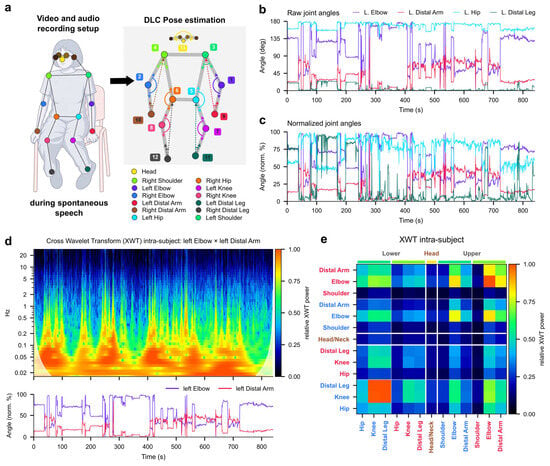
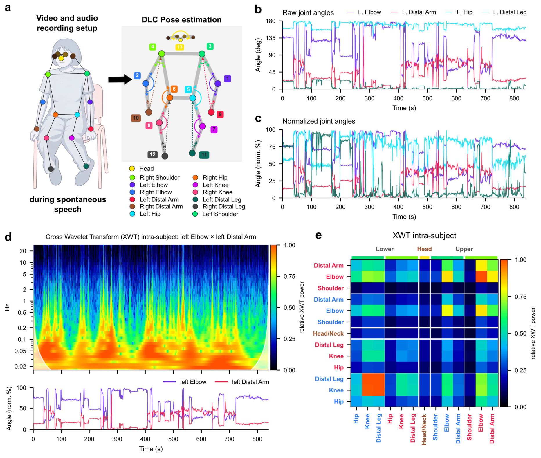
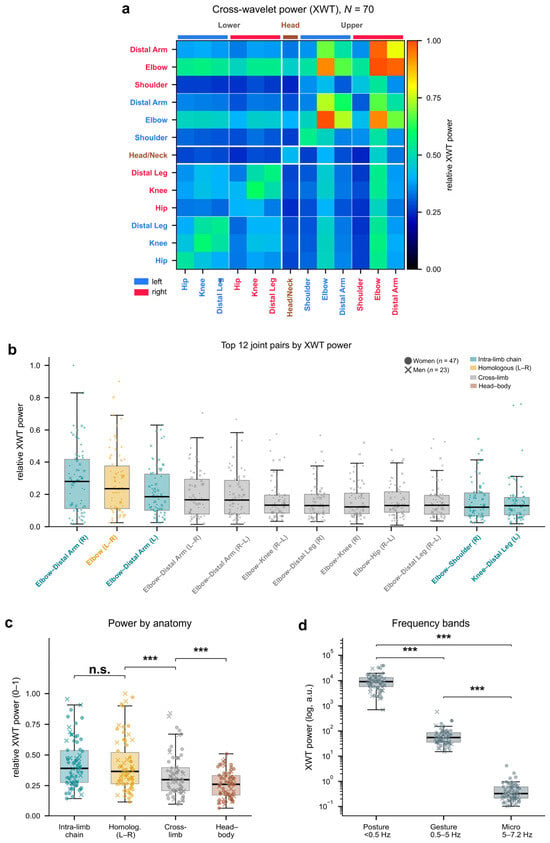
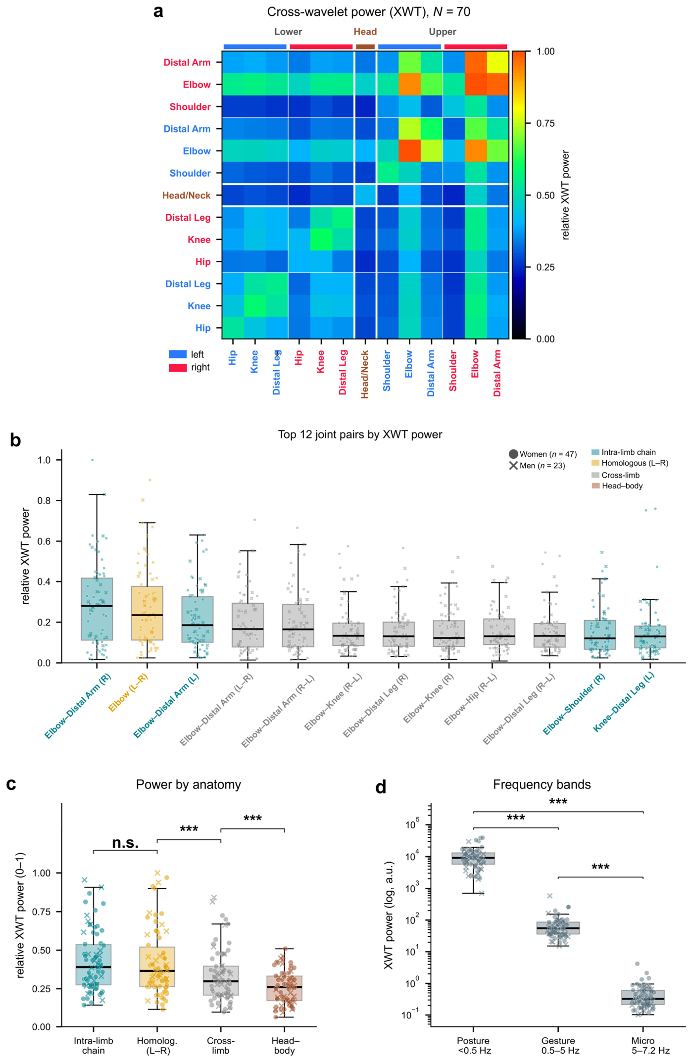
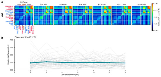
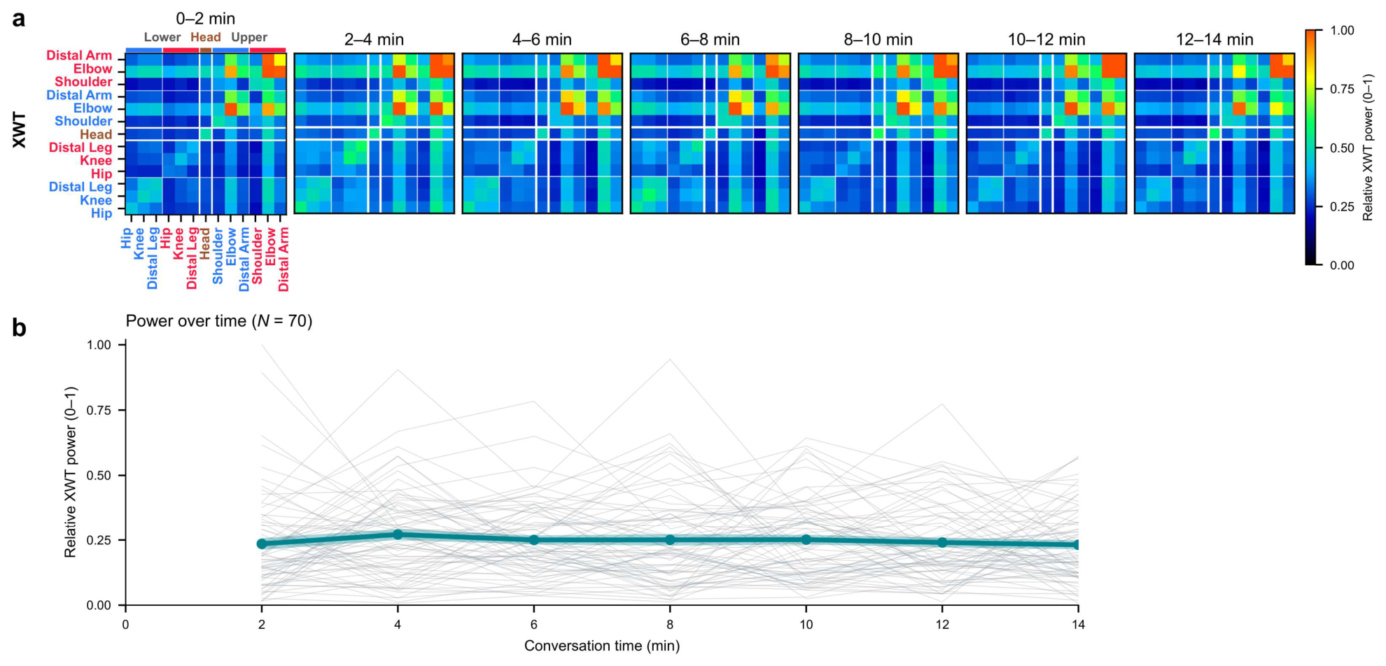
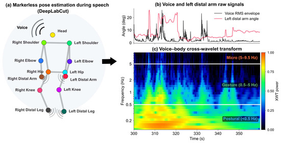
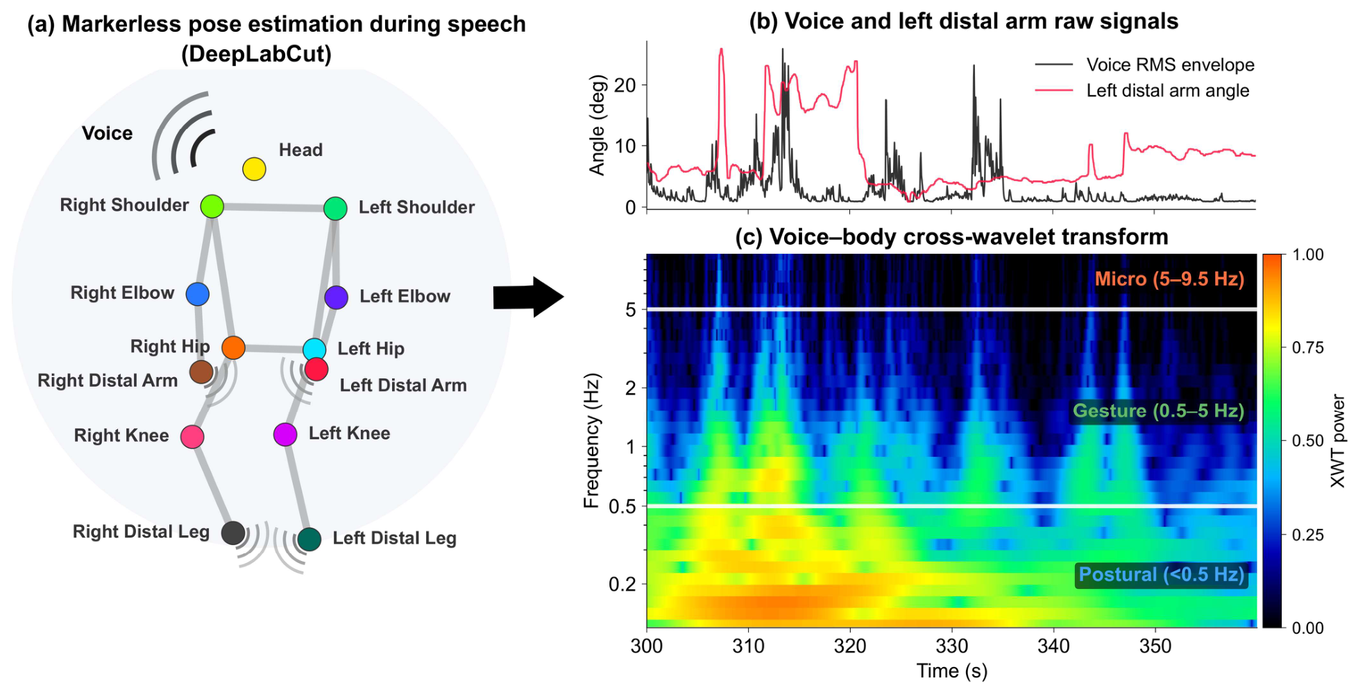
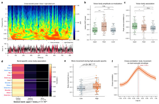
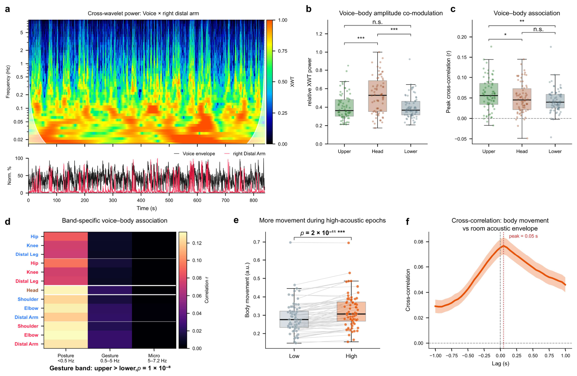
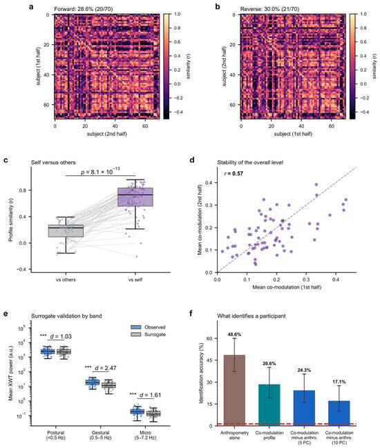
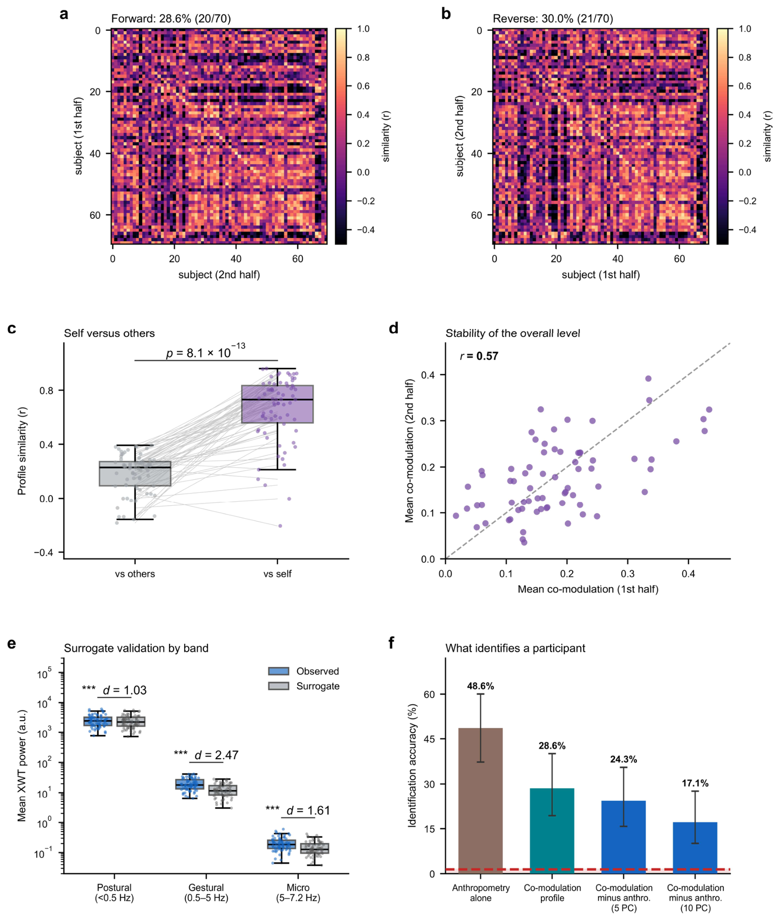

Disclaimer/Publisher’s Note: The statements, opinions and data contained in all publications are solely those of the individual author(s) and contributor(s) and not of MDPI and/or the editor(s). MDPI and/or the editor(s) disclaim responsibility for any injury to people or property resulting from any ideas, methods, instructions or products referred to in the content. |
© 2026 by the authors. Licensee MDPI, Basel, Switzerland. This article is an open access article distributed under the terms and conditions of the Creative Commons Attribution (CC BY) license.