


Abstract
Part segmentation of industrial 3D models is often limited by the lack of sufficiently large and consistently labeled training datasets. This study proposes a workflow for generating synthetic segmentation datasets from robust parametric computer-aided design (CAD) models and evaluates its applicability on a dental abutment case. The workflow includes the definition of a modeling strategy, creation of a robust parametric CAD model, automated generation of valid geometry variants, and preparation of labeled training data for point-cloud-based segmentation. In the experimental part of the study, a synthetic dataset of segmented dental abutment geometries was generated from the developed parametric CAD model and used to train a PointNeXt-S part-segmentation model. The segmentation performance of the trained model was evaluated on manually labeled real-world abutments. Results show that the segmentation of industrial 3D models improved with increasing synthetic training-set size and further improved when data augmentation was applied. The best-performing augmented model achieved a mean Intersection over Union (IoU) of 89.2% on the real-world validation set, compared with 82.4% without augmentation. The findings indicate that parametric-CAD-based synthetic dataset generation can provide an effective basis for training segmentation models for complex industrial geometries.
1. Introduction
3D model segmentation is an important task performed across the fields of computer-aided design (CAD), computer graphics, and other engineering applications such as preparing models for manufacturing and assembly (detecting, e.g., holes, profiles and flat surfaces). In simple terms, segmentation assigns labels to the elements that make up the 3D object (points, pixels, faces, and similar). It supports not only geometry-based work, such as machining, surface analysis, and inspection, but also function-oriented tasks such as grasping, positioning, joining, and assembly. In industrial workflows, segmentation can therefore include more than a characteristic geometry recognition step.
Given its implications, segmentation has been the subject of many research studies that were focused on developing new architectures to overcome specific limitations or problems that arise from previous studies or specific usage. Interestingly, most of these architectures were validated on benchmark datasets. Generally, benchmark datasets are curated collections of data, such as 2D images or 3D models, used to test and validate algorithms on specific tasks such as part segmentation, instance segmentation, and semantic segmentation. Their main advantage is that they enable direct comparison between methods (such as training time and segmentation evaluation metrics). In 3D model segmentation, benchmark datasets typically include classes such as airplanes, cars, and chairs, with preprocessing procedures that are well documented. The most common one is ShapeNetPart [1], and many studies related to the development of part segmentation models, including PointNet, PointNet++, and PointNeXt [2,3,4], reported the use of this or similar datasets as baselines. While such benchmark datasets are useful for comparing methods under controlled conditions, they do not completely reflect the characteristics of models that are typically handled in industrial applications.
Whereas benchmark datasets and related problems and solutions have been well documented, the industrial datasets introduce case-specific challenges. Industrial collections of 3D models often contain multiple variants of products from the same product family. Geometrical differences between variants can be difficult to detect (in contrast to benchmark datasets containing objects such as cars, planes and chairs), but they can still be important for function and fit in relations to other components. At the same time, real industry datasets commonly do not contain enough data for accurate training, which limits the direct use of data-hungry deep learning models [5]. Another issue is data inconsistency [6]. Namely, as industrial 3D models are often created in different CAD systems and use different export settings, the collected files can differ a lot even when they represent the same type of part. Such inconsistencies may appear as differences in model orientation and representation detail. For example, the same part may be exported in different coordinate orientations [7], while small geometric features such as holes, filets, chamfers, or internal structures may be retained in some files but simplified or omitted in others [8]. Additionally, conversion from CAD to mesh formats, which are typical for deep learning applications, can also introduce errors and artifacts.
Even when the datasets are geometrically preprocessed, their labeling is often the main bottleneck. Depending on the objective of the study, segmentation labels may be defined according to geometric form, manufacturing features, or functional role [8,9]. Here, functional segmentation implies the assignment of labels to part regions according to their engineering role in use or assembly, rather than solely according to geometric form. Therefore, the goal of conducting functional segmentation in an industrial context is often to identify regions that matter for use, positioning, or joining. Accordingly, labels are assigned based on the role that a region plays in the product, for example, as a contact surface, positioning feature, sealing area, or joining interface [10,11]. Defining such labels typically requires domain expertise, which makes manual annotation time-consuming and difficult to scale. A limitation reported in prior work is that many CAD segmentation approaches are geometry-driven, relying on curvature, normals, or fitted primitives to partition models into homogeneous regions [12,13,14]. However, function-oriented segmentation addresses a different objective—one that does not relate only to geometric form [10,15]. Although geometry-driven partitioning can indeed be useful for manufacturing-oriented tasks such as automated process planning, sheet metal tool design, die/mold machining, or refinement of finite element meshes, it cannot fully support tasks that rely on identification of functional segments of 3D objects [14]. These functional segments do not always coincide with geometric primitives, because they are defined by engineering role rather than solely by local shape. Their interpretation often depends on context, such as the part’s position in the assembly, its contact with neighboring components, or its role in joining, sealing, or load transfer.
Taken altogether, the challenges related to data heterogeneity, functional labeling requirements, and manual annotation effort define a clear research gap when it comes to segmentation of real-world CAD data. Prior work has addressed these challenges by investigating the opportunity of utilizing CAD-based synthetic data to reduce manual annotation effort and enable controlled variation in industrial machine-learning pipelines [7,16,17]. Despite demonstrating the potential, these studies also highlight the gap between synthetic and real data, including differences in data distribution, labeling conventions, and realism [5,6,17]. Hence, concrete evidence remains limited for workflows that translate CAD-based synthetic data generation into function-oriented segmentation of industrial 3D parts under real deployment conditions. In particular, there is still a lack of workflows that perform well when only limited numbers of annotated real samples are available and when the target data are both inconsistent in representation and heterogeneous in product geometry and functional segmentation patterns. To address this gap, this study proposes a structured workflow that generates synthetic training data from a robust parametric CAD model and uses this dataset to train a segmentation model. Rather than introducing a fundamentally new synthetic data generation algorithm, the contribution lies in the methodical integration of existing CAD-based synthetic data principles into a robust, segmentation-training-ready workflow, including parametric generation of large numbers of valid geometry variations, explicit handling of parameter dependencies and dynamic parameter ranges, and validation on real industrial data. The main contributions of the presented work are: (1) a structured method for generating segmentation-training-ready synthetic datasets from robust parametric CAD models, with particular emphasis on maintaining valid geometry variation through parameter dependencies and dynamic parameter ranges; and (2) empirical insights from an industrial case study into how such a workflow performs under real-world conditions, including its practical applicability and segmentation performance on real industrial data.
2. Background
Recent advances in machine learning, and particularly deep learning, have enabled learning-based segmentation approaches that are now widely used in 3D geometry data analysis [18]. For a better understanding of functional segmentation challenges, especially those related to 3D geometry data and the use of synthetic datasets to improve segmentation performance, this section provides a brief overview of the theoretical background. The section is divided into three main parts. The first subsection presents an overview of segmentation algorithms, with a particular focus on point cloud-based approaches. This focus was adopted because point cloud representations have been widely used in learning-based 3D segmentation and form the basis of many state-of-the-art architectures. The second subsection discusses the use of synthetic datasets for segmentation purposes, highlighting their advantages and limitations in the context of training deep learning models. The last subsection reviews several existing modeling strategies for generating synthetic datasets and highlights the importance of preparing robust parametric CAD models.
2.1. Segmentation Algorithms for 3D Point Clouds
In general, segmentation is the task of assigning a label to individual elements of a visual or geometric representation, such as pixels in an image or points in a point cloud [3]. In the literature on 3D point cloud analysis, segmentation tasks are commonly divided into three categories: semantic segmentation, part segmentation, and instance segmentation [2,19]. Semantic segmentation assigns each point or pixel to a class describing the type of object or region to which it belongs, such as floor, wall, chair, or car. Whereas semantic segmentation focuses on scene-level understanding, part segmentation focuses on the object level, where each point or pixel is assigned to a label corresponding to a constituent part of the object [2]. In contrast, instance segmentation distinguishes between separate objects belonging to the same class; for example, if a scene contains five cars, each car is identified and labeled as a separate instance [19]. Depending on the study objective, such segmentation labels may be defined primarily according to geometric characteristics or according to the functional role of the identified region.
Three-dimensional scenes and objects can be represented in several different ways, such as point clouds, voxel grids, meshes, or multi-view projections. In this study, the focus is on point cloud data representation, which is an unordered set of points in 3D space [2]. Point clouds are often obtained as raw outputs from 3D acquisition devices, such as Light Detection and Ranging (LiDAR) scanners, but they can also be generated based on other 3D representations, such as CAD models [3,20]. Point cloud models typically require relatively low computational resources for storage and analysis, which is a major advantage when large amounts of data are used for training neural network algorithms [21]. However, in their basic form, point clouds do not contain explicit information about connectivity between points or about which points are true local neighbors, which can be a major limitation [22]. This directly influences segmentation performance and motivates the use of point cloud-specific segmentation approaches [23]. Many segmentation algorithms are primarily developed for semantic segmentation, but they can often be adapted to part segmentation by redefining the target labels at a finer level of granularity and adjusting the training setup accordingly. While part-category labels may overlap with functional segments of a specific object, this study focuses on part segmentation and point cloud architectures that are commonly evaluated on part segmentation benchmarks.
One of the point cloud architectures, which has served as a foundation for several later extensions, is PointNet [2]. For part segmentation of ShapeNetPart benchmark models, PointNet reported 83.7% mean Intersection over Union (mIoU) [2], which is one of the commonly used metrics for segmentation performance, together with overall accuracy (OA) and mean accuracy (mAcc), depending on the dataset and task [2,4]. One of its most notable extensions has been PointNet++, which addressed a key limitation of the original architecture, namely its limited ability to model neighborhood relations and local geometric structure among nearby points, which is important for recognizing fine-grained shape patterns, especially in complex scenes [3]. PointNet++ introduced a hierarchical feature learning framework built using Set Abstraction (SA) layers. Each SA layer consists of three components: a Sampling layer, a Grouping layer, and a PointNet layer. Using this hierarchical framework, PointNet++ reports improved performance (85.1% mIoU) for part segmentation when applied to the ShapeNetPart benchmark dataset [3]. Several later architectures build on this hierarchical feature-learning strategy, which captures local geometric features through multi-level grouping of points. The most notable has been PointNeXt, which represents a modernized version of PointNet++, with improvements based on receptive field scaling and model scaling [4]. Key improvements introduced include an inverted residual bottleneck design, separable multi-layer perception networks (MLPs), and residual connections within the SA blocks. The architecture is also scalable, allowing adjustment of the MLP channel size and the number of InvResMLP blocks. The PointNeXt family consists of four model variants that differ in network width and depth, specifically in the base channel size and in the number of InvResMLP blocks used at each stage. Based on these improvements, 87% mIoU is reported for part segmentation on the ShapeNetPart dataset [4].
Several additional algorithms use PointNet-based architectures as a backbone or reuse specific blocks from the PointNet family. SGPN uses PointNet++ to extract a feature matrix, which is then passed through three parallel branches to generate a similarity matrix, a confidence map, and a semantic segmentation map [24]. Using this architecture, SGPN reported 85% mIoU on part segmentation for the ShapeNetPart dataset [24], which the authors describe as a 1.2% improvement over PointNet++ under their experimental setup. Similar to SGPN, AKDNet uses PointNet++ as a feature extractor. Within AKDNet, a KNNGraphConv-based module is used to refine and augment the features extracted from PointNet++ [18]. On the ShapeNetPart benchmark, the full AKDNet model reported 85.83% mIoU [18].
While some architectures reuse complete PointNet or PointNet++ pipelines as a backbone, others adopt only selected modules or use similar design principles. One example is SO-Net [25], in which the point cloud is first processed using a Self-Organizing Map (SOM), and features are then extracted from the resulting mini point clouds using a local PointNet-like module. For part segmentation of the ShapeNetPart dataset, SO-Net reported 84.6% mIoU [25]. Another architecture inspired by PointNet is DGCNN [26] which constructs a local neighborhood graph and applies convolution-like operations on edges between neighboring points, rather than processing points independently. On the same dataset, DGCNN reported 85.2% mIoU [26].
Beyond PointNet-related designs, alternative point-cloud architectures have also been proposed for segmentation. One example is SpiderCNN, whose fundamental building block is SpiderConv [27]. Through this block, filters are chosen from a parameterized family, and parameters are optimized using the SGD algorithm. Using this algorithm, an 85.3% mIoU was reported on the ShapeNetPart dataset. To overcome problems with local feature extraction, OECNN proposes improved orientation-encoding convolution and pooling strategies [28]. This architecture adopts a selective top-k pooling strategy from SpiderCNN. When this architecture was applied to the ShapeNetPart dataset, an 85.5% mIoU was recorded.
In summary, the reviewed architectures show that substantial progress has been made in point-cloud-based part segmentation, particularly through improved learning of local geometric features. However, these advances are largely demonstrated on benchmark datasets with abundant annotated data and, therefore, do not directly resolve the challenges of industrial functional segmentation. As a result, the question of how to obtain suitable training data remains central, which motivates the next subsection on synthetic datasets.
2.2. Synthetic Data for Segmentation
Synthetic datasets are collections of data generated using computer algorithms. In the context of segmentation, each point, pixel, or other element of the generated representation can be automatically assigned an annotation and a ground-truth label, because the underlying scene structure is known by construction. This differs from many real-world applications, where datasets must first be collected and then manually labeled, which is time-consuming and can introduce inconsistencies between annotators or across labeling sessions. As a result, synthetic data generation can reduce labeling effort and enable large-scale dataset creation under controlled conditions. Depending on the dataset’s main application, output data representation and additional modalities can differ. In general, synthetic datasets for part segmentation can contain 2D images [29], RGB-D images [7], or 3D objects [30]. However, the usability of synthetic data for real applications depends on how well the generated data represent the variability and noise characteristics of the target domain, and this is often discussed as a synthetic-to-real domain gap [31].
Synthetic data generation has been widely explored in prior studies, particularly through 2D image-based pipelines. In such approaches, images are typically rendered from CAD models or synthetic scenes under controlled illumination, materials, backgrounds, and virtual camera settings, while pixel-level ground-truth labels are generated automatically. A representative example is the SYNTHIA dataset, which provides a large collection of synthetic urban scene images for semantic segmentation [29]. In industrial applications, several pipelines and toolkits have focused on CAD-to-render workflows to generate photorealistic training data under controlled conditions [32,33]. In addition, comparative studies indicated that different synthetic data sources and generation strategies (e.g., CAD models, 3D scans, or hybrid approaches) can influence downstream model performance and transfer to real-world data [5]. Although such 2D synthetic data generation can significantly increase the amount of labeled training data, its effectiveness depends on the synthetic-to-real domain gap and on how well the generated images capture the variability of the target domain. Since this study focuses on 3D point cloud part segmentation, the following paragraphs discuss strategies for generating synthetic 3D datasets, with an emphasis on CAD-based generation and point cloud representations.
Synthetic 3D datasets can be generated from different 3D sources, depending on the target task and the required level of fidelity. One approach is based on real 3D scanned objects, where high-quality scanned models are collected and then used as assets in simulation environments [30]. Another approach relies on fully virtual environments, where labeled point clouds are generated by simulating sensors and scanning procedures. For example, synthetic city-scale point clouds can be generated using simulated mobile laser scanning in a virtual scene [34]. Similarly, synthetic LiDAR sequential point clouds can be generated across multiple virtual environments, with point-wise semantic labels assigned during generation [17].
In industrial applications, CAD models are often used as a base for synthetic data generation. In this case, CAD files and material properties can be imported into a generation pipeline, different environment settings can be applied, and annotated datasets can be produced under controlled conditions [32]. Besides fixed generation settings, some works proposed optimization-driven approaches, where parameters of the simulator are tuned in a closed loop to improve the usefulness of synthetic point clouds for training segmentation models [31]. Hybrid pipelines also exist, in which CAD files and models reconstructed from real scans are combined within simulation engines to generate randomized datasets for downstream tasks. These studies indicated that CAD-based models, 3D scans, and hybrid approaches can lead to different trade-offs in realism, scalability, and ability to transfer to real-world data [5].
However, regardless of the generation strategy used, an important limitation remains: the quality and usefulness of synthetic data depend strongly on how systematically geometry variations and part-level labels can be controlled. In scan-based approaches, the underlying geometry is typically fixed, which limits the generation of large numbers of controlled shape variants. In many virtual-scene-based pipelines, by contrast, the main focus is on scene-level semantic labeling, where points are assigned broad object-class labels, rather than on consistent part-level segmentation across systematically varied object geometries. This creates a gap for part-segmentation applications, where large amounts of consistently labeled data are needed across a wide range of geometry variations. A parametric CAD model provides a practical basis for addressing this gap, because it enables systematic and repeatable generation of geometry variations while preserving both part definitions and their associated labels. In this way, it supports scalable synthetic dataset generation for part segmentation and enables a controlled evaluation of how segmentation performance changes across valid geometric variants.
2.3. Parametric CAD Modeling Strategy
When a parametric CAD model is used for automatic generation of a large number of geometry variants (geometry differences produced by CAD model parameter changes), the modeling strategy becomes important because it directly affects flexibility, reusability, and the ability of the model to regenerate after parameter changes [35]. In this context, a model that works well for a single design instance can become unstable when parameters are systematically sampled and the geometry must be rebuilt repeatedly [35]. The literature therefore treats modeling strategy, including the way features, references, parameters, and constraints are organized within a model, as a key factor for creating reusable parametric models and enabling practical large-scale variation generation in workflows such as design optimization [35,36].
A stable parametric CAD model is essential for automated pipelines, because regeneration can fail for certain parameter combinations and thereby interrupt large-scale variant generation [35]. In the literature, such stability has been mainly linked to the way feature dependencies, references, constraints, and parameter ranges are structured within the model [35,37]. In particular, fragile parent–child relations between features, complex or poorly organized dependency chains, redundant or under-/over-constrained sketch profiles, and change-sensitive local operations such as filets and chamfers have all been found to increase the likelihood of regeneration failure [35,36,38]. Stability can also be affected by the definition of the design space itself, since overly broad or poorly formulated parameter ranges may lead to geometrically invalid or topologically inconsistent model instances. In this context, valid parameter ranges refer to parameter intervals for which the model can regenerate successfully while preserving a closed and intended geometric form, whereas robust modeling practices refer to strategies for organizing references, constraints, and feature dependencies so that the model remains reusable and resilient under repeated parameter changes [35,37,39].
To address these regeneration and reuse challenges, several modeling strategies were proposed, which differ in how they organize references, dependencies, and change propagation within a parametric CAD model. Feature-based history modeling has been widely used, but its robustness can decrease when later features depend strongly on earlier ones and parameter changes propagate through long dependency chains [35,36,37]. Reference-based approaches, including Explicit Reference Modeling (ERM) and related methodologies, seek to reduce this sensitivity by grounding features in stable reference entities such as planes, axes, and points, and by limiting dependencies on previously created geometry [35,36]. Similarly, top-down strategies improve predictability by using a stable skeleton or layout to control global parameters and propagate change in a structured way, whereas bottom-up strategies construct geometry locally and may become less predictable as constraints and feature interdependencies grow in complexity [35,36]. Another relevant aspect is the treatment of sketch constraints: the elimination of redundant constraints was found to reduce solver complexity, lower the risk of regeneration errors, and improve model robustness when profiles are edited, reoriented, or reused in automated workflows [38]. In addition, algorithmic parametric modeling introduces rule-based or visual-programming procedures that automate the generation of multiple valid design variants from predefined parameter logic, which is particularly relevant when large numbers of geometrically valid instances must be produced systematically [40].
Taken together, these studies demonstrated that robust synthetic dataset generation from parametric CAD models depends not only on the existence of adjustable parameters, but also on the way references, dependencies, constraints, and variation logic are structured. However, the literature still provides limited guidance on how such modeling principles can be translated into workflows for generating consistently labeled geometry variants for part-segmentation training and validation under controlled industrial conditions.
3. Method
The proposed method aims to provide a systematic workflow for the generation of synthetic datasets, followed by the training of deep learning algorithms for part segmentation. As mentioned, the main advantage of using synthetic datasets arises in the context of 3D model segmentation, where manual preparation of training data is both time-consuming and prone to inconsistencies, or even infeasible when 3D models cannot be prepared with sufficient accuracy and consistency. The proposed workflow is divided into three main phases, illustrated in Figure 1, highlighting the sequential nature of the method: (1) parametric CAD modeling, (2) synthetic dataset generation and (3) deep learning model training.
Figure 1.
The sequential workflow of the proposed method.
3.1. Parametric CAD Modeling
The first phase of the proposed method focuses on defining a robust parametric CAD model that enables the systematic generation of geometry variants. This phase is divided into two steps: (1.1) modeling strategy definition and (1.2) parametric CAD model creation.
3.1.1. Modeling Strategy Definition
When simple 3D models can be defined using a small number of parameters and the associated geometries are simple (e.g., cylinders or basic filets), robust parametric CAD models (i.e., models that regenerate correctly when parameters are changed within defined ranges [35]) can often be created without a strongly defined modeling strategy. However, in the context of complex 3D models, where many related parameters are needed to define complex geometries, defining an appropriate modeling strategy is crucial. When parameters are changed, geometric dependencies can lead to regeneration errors or unrealistic geometry, for example, due to missing or unstable reference entities, invalid intersections, or topology changes that break feature dependencies. Hence, the main purpose of this step is to plan the modeling process so that it results in a robust parametric CAD model.
To achieve this, an adapted horizontalized explicit reference modeling methodology (ERMM) was used [37]. While ERMM was originally defined for solid-based parametric modeling, in this work the modeling strategy is also extended to parametric surface-based modeling. The modeling strategy definition consists of five sub-steps: parametric CAD software selection, definition and modeling of functional geometries, definition of relations between functional geometries, parameter identification and classification, and definition of parameter relations, equations, and parameter ranges.
Before modeling the functional geometries, appropriate parametric CAD software must be selected based on geometry complexity, the intended modeling approach, and the need for stable regeneration across geometry variants. Geometry complexity is important because simple geometries can often be modeled using standard parametric operations, whereas complex free-form or highly detailed shapes may require advanced surfacing tools, more flexible reference handling, and finer control over local shape definition. The selected CAD system must therefore support the type of modeling most suitable for the case, whether solid-based, surface-based, or a combination of both. Solid-based modeling is often suitable when the geometry can be represented as closed volumes and when feature operations such as extrusions, cuts, patterns, and blends can be defined in a stable way. Solid models are also practical when a consistent volumetric definition is required. Surface-based modeling is often more suitable for complex free-form geometries, because the geometry can be built as a controlled set of surfaces in which local shape is managed through curve definitions and surface continuity. According to the VDI 2209 guideline, surface modeling is used mainly when volume-oriented modeling is not appropriate, for example, for sheet metal parts and automotive bodies, when locally complex areas must be modeled separately, such as castings and forgings, or when production-related aspects require separate surface definition, as in mold and die making [36]. In addition, surface modeling is typically used when arbitrary or highly complex shapes must be controlled, especially in domains such as automobile, aviation, and ship-building industries [41]. At the same time, the chosen CAD tool must support stable regeneration under repeated parameter changes, since trimming, surface intersections, feature dependencies, or surface knitting operations may fail when geometry varies significantly across generated variants. For this reason, the modeling approach should be selected according to geometry complexity, required shape control, and regeneration robustness under parameter changes.
The CAD software selection should therefore be aligned with the requirements of robust parametric modeling, namely the ability to define and manage parameters, equations, references, and feature dependencies in a way that supports stable regeneration under repeated parameter changes. In particular, the software should allow parameter relations to be implemented without unstable references, such as dependencies on edges, faces, or intermediate features that may disappear or change when the geometry is modified. It should also support repeated parameter updates and predictable model regeneration, especially in models that contain complex surfaces or long multi-step feature histories. Additionally, the selected CAD software should enable controlled export of generated geometry variants in appropriate file formats and representations, such as boundary representations or mesh-based outputs, depending on the requirements of the downstream workflow.
To enable the structured creation of a parametric CAD model in the selected CAD software, the modeling strategy definition starts by dividing the complete 3D model into functional geometries. Following the ERMM, each functional geometry is defined as independently as possible, with minimal dependencies on other functional geometries, in order to reduce parent–child relations and limit error propagation during regeneration [35]. For example, in a working desk, functional geometries can include the desk leg, the tabletop, and the storage space. In the case of complex free-form geometries, the corresponding CAD model can require too many dimensions and relations, which makes it overly complex and difficult to convert into a robust parametric CAD model. In such cases, simplifications to the original geometry can be introduced on the basis of functional relevance and parametric robustness, by retaining shape features that define the part’s role and appearance while reducing details that unnecessarily increase modeling complexity or regeneration instability. When geometry is simplified, the overall form of the part and the geometric features that are essential for its functional role and segmentation labeling should be retained as much as possible [36]. For example, when an original surface requires a large number of complex curves, a simplified surface can be modeled using only a few representative curves while preserving the functional role and the overall form and segmentation-relevant geometric features of that surface. For each functional geometry, a separate CAD model is first created without defining parameters or relations between parameters.
Once the functional geometries are modeled, the geometric relations between them can be defined. Through this sub-step, functional geometries are assembled into a complete model while maintaining consistent interfaces and alignment conditions. In the working desk example, the screw holes on the desk leg must be concentric with screw holes on the tabletop.
After the complete model is assembled, the required parameters should be identified and classified. Each identified parameter can be classified into one of three categories: (1) input parameter (directly assigned by the user or another algorithm), (2) equation-driven parameter (calculated based on the value of one or more other parameters), and (3) parameter with fixed value (kept constant across all generated variants). Input parameters are those that directly influence product functionality and are intended to be varied by the user or by automated procedures such as optimization or generative algorithms. For the working desk example, table length and width can be treated as input parameters because they define the usable work surface and the fit of the desk into a workspace. Equation-driven parameters are those whose values depend on one or more other parameters, such as the positions of screw holes defined relative to the table dimensions and leg thickness. Finally, parameters with fixed values remain constant across all generated variants, for example, a fixed tabletop thickness.
The last sub-step of the modeling strategy definition concerns the equations and dependencies that relate to parameters. At this stage, redundant parameters can also be identified and removed, because after the separately modeled functional geometries are assembled into a complete model, the same geometric relation may be represented by multiple local parameters originating from different functional geometries. Here, input parameter ranges are also defined to support systematic variant generation while avoiding unrealistic or invalid configurations. For synthetic dataset generation, the parametric CAD model should be based on a limited number of necessary input parameters and should avoid unnecessary geometric detail, redundant dependencies, and overly complex feature relations, while still producing valid geometry and preserving functional characteristics. This modeling strategy definition therefore establishes the basis for robust large-scale generation of geometry variants for subsequent dataset creation.
3.1.2. Defined Modeling Strategy Evaluation
Once the modeling strategy has been defined, the next step is to create a robust parametric CAD model in the previously selected CAD software. In the preceding step, CAD models were created separately for each functional geometry to define their intended shape and role. In this step, these functional geometries are integrated into a single parametric CAD model that serves as the baseline for systematic variant generation. The primary objective is to implement the defined modeling strategy in a way that allows parameters and their interdependencies to be modified reliably, without regeneration failures.
In this implementation step, fixed dimensions are replaced by named input parameters, while dependencies between functional geometries are realized through stable references, interface-defining constraints, and equation-based parameter relations. To maintain regeneration stability, unnecessary geometric detail, redundant parameters, and fragile dependency chains are avoided as far as possible. Where parameters are not independent, equation-driven relations are introduced to enforce the intended constraints and preserve valid parameter combinations during regeneration. This includes linking coupled dimensions and embedding design rules that prevent inconsistent or infeasible configurations.
In addition, the model is prepared with downstream data generation in mind. Although the functional geometries are initially integrated into a single parametric CAD model so that their relations, interfaces, and shared parameter dependencies are preserved, they must later be exported individually for dataset generation and labeling purposes. For this reason, the feature tree is organized so that features belonging to each functional geometry remain grouped and can be isolated, regenerated, and exported with minimal side effects on the rest of the model. This feature-tree organization improves the traceability of parameter effects, supports repeatable exports, and contributes to the overall robustness of the parametric CAD model.
3.2. Synthetic Dataset Generation
Once the robust parametric CAD model is completed, it can be used to automatically generate a diverse synthetic dataset of geometrically valid CAD model variants. To achieve this, input parameters are randomly sampled within their predefined ranges, and each sampled parameter combination is used to regenerate a CAD model variant. In this way, multiple variants are generated to cover the intended design space of the 3D geometry. This approach allows the generation of a large number of models in a consistent and repeatable way, which is important for further training and evaluation of deep learning algorithms.
In addition to fixed parameter ranges, some parameters require dynamic ranges whose limits depend on one or more other parameter values. Such dynamic ranges cannot be defined directly in the parametric CAD model and must therefore be implemented in a user-defined automation script that updates input parameters and triggers model regeneration. In such cases, the parameters form a dependency hierarchy, in which the value of one parameter determines the feasible range of another. Parameter values are therefore assigned sequentially, starting from independent parameters and continuing toward dependent parameters whose admissible ranges can only be computed after upstream values are known. For example, if a hole is generated on a host face, the maximum hole diameter depends on both the hole position and the dimensions of the host face. First, the host-face dimensions are assigned independently within fixed ranges. Based on these values, the feasible limits for the hole position are calculated, and the hole position is then selected within the updated range. The hole diameter is then determined from the hole position and the host-face dimensions, while also considering the remaining material between the hole boundary and the surrounding face edges. As the final step, the diameter value is selected within the calculated range. This sequential procedure ensures that parameter combinations remain feasible and that the resulting geometry does not contain unrealistic or invalid features during automated variant generation.
First, a list of valid parameter combinations is generated according to the predefined fixed and dynamic parameter ranges, including the dependency rules between parameters. Then, each valid combination is applied sequentially to regenerate a CAD model variant, which is automatically exported in the required format using the integrated export functions of the CAD software, additional plug-ins, or external scripts. The exported files must be organized in a consistent folder and metadata structure so that each geometry variant can be traced back to its input parameters and used efficiently in later preprocessing, training, and evaluation steps. Geometry files can thus be stored in separate folders according to the CAD model variant or geometry class, while the corresponding parameter values can be saved in a separate metadata file when required. In the working-desk example, each functional geometry, such as the desk leg or tabletop, can be exported as a separate 3D model in STEP or stereo lithography (STL) format, while all files belonging to one variant are stored in a folder with a specific name. In this case, each folder represents one geometry variant, and the STL files stored within it each represent one functional geometry. In the segmentation context, each of these files can additionally be assigned a segment label.
In some cases, additional dataset augmentation is required to expand the dataset, increase the diversity of geometry variants, and improve the robustness of the training process. In general, augmentation methods can be divided into basic and specialized techniques [42]. Additionally, advanced augmentation frameworks have also been proposed, such as PointAugment, LidarAugment [42], and auto-augmenter for images and meshes (AIM) [43]. Basic augmentation techniques include translation, rotation, and scaling, whereas specialized techniques include operations such as point or region erasing and the application of small random perturbations to point coordinates, in order to simulate noise, minor geometric deviations, or sensor-related inaccuracies [42,44]. Depending on the structure of the real dataset and the target segmentation task, certain augmentation methods may have no positive effect or can even reduce the segmentation accuracy [4,42]. For example, in cases where all 3D geometries in real datasets are aligned, augmentation with additional rotation or translation does not have a positive impact on part segmentation model performance. In other cases, where real-world datasets are collected by sensors such as LiDAR, thereby including noise and small deviations from expected geometry, the augmentation using small perturbations or deleting some points or regions can have positive effect on model performance.
3.3. Deep Learning Model Training
The generated synthetic dataset consisting of 3D geometries of individual functional geometries is not directly suitable as a training input for segmentation networks. The dataset must first be converted into the input representation required by the selected part segmentation model. In this step, the separately exported functional geometries are combined into the complete labeled geometry representation required for training, and each geometry is assigned its corresponding segment label. The assembled geometry is then converted into training samples (depending on the chosen approach, this can be done as point-based samples, mesh-based samples, or another compatible representation). For each training sample, the corresponding ground-truth labels are stored so that the network can learn the segment label of each point, face, or other unit of the chosen input representation.
Deep learning architectures used for segmentation are selected primarily according to the representation type of the available data and the segmentation task. When synthetic datasets are used, model selection should also consider how well the chosen architecture matches the generated data representation and how suitable it is for transfer to the target real dataset. The primary condition for selecting a segmentation architecture is the required data representation; for example, mesh-based architectures cannot be applied to point-cloud datasets. Additionally, some architectures are presented together with benchmark-specific implementations and training settings. Therefore, results reported on benchmark datasets that are most similar to the target case can be used as an initial reference during model selection. For example, if the real-world dataset consists of 3D models of objects such as tables or chairs, an architecture that reports strong performance (e.g., evaluation metrics and training time) on a dataset such as ShapeNetPart may be an appropriate starting point. When the target task is part segmentation, the output classes should correspond to the predefined segment labels. The selected model should therefore be trained on the generated synthetic dataset with an output layer whose size matches the number of labeled segments. Prior to training, the dataset should be divided into training and validation sets. A common approach is random splitting, for example, into 80% training and 20% validation data, although the ratio may be adjusted to the specific case. The training set is used to optimize the model weights, while the validation set is evaluated at the end of each epoch and used for model selection and hyperparameter tuning, such as learning-rate adjustment. Both splits may also require preprocessing, such as format conversion between representations, depending on the chosen data representation and the model requirements.
The training procedure follows a supervised training protocol appropriate for the selected segmentation architecture, such as the training settings reported for PointNeXt on the ShapeNetPart dataset [4]. Model-specific training settings should be defined according to the selected architecture and benchmark training protocol, for example, the optimization setup, augmentation strategy, and training schedule reported for comparable part-segmentation models [4]. When synthetic datasets are used, the training procedure should also account for the synthetic-to-real domain gap, for example, by incorporating the aforementioned augmentation or domain-randomization strategies that reflect the variability and noise characteristics expected in the target real dataset. Performance is monitored on the synthetic validation set using IoU and mIoU. IoU measures the overlap between predicted and ground-truth labels divided by their union, while mIoU is computed as the mean IoU across all classes.
After training, the model should also be validated on real-world data. This step is used to assess whether the generated synthetic dataset adequately captures the characteristics of the expected real data. In this way, the practical usefulness of the proposed dataset-generation workflow can be verified. For this purpose, the trained segmentation model is evaluated on labeled real-world samples using the same performance metrics. An example of a concrete implementation of this procedure is described in the Experiment section.
4. Experiment
The experiment was conducted to verify the applicability and performance of the proposed method under real conditions. As such, it included generating a synthetic dataset based on a parametric CAD model, training a segmentation model using this dataset, and then assessing whether the trained model can be applied to a real industrial dataset.
The method described in Section 3 was implemented on a representative industrial case, i.e., a dental abutment, to demonstrate the feasibility of the complete workflow. This case exhibits both the lack of labeled and systematically organized real data for training segmentation models and a complex geometry including free-form surfaces and poorly defined segment boundaries. Namely, the boundary between certain segments of a dental abutment can be difficult to define consistently, especially when the segmentation is performed manually by multiple operators. In addition, manual segmentation of a single model can take 10–20 min, which results in substantial preparation effort when hundreds or thousands of models must be processed. These characteristics make the abutment case suitable for evaluating a systematic and repeatable method for generating segmented training data while reducing manual effort and labeling inconsistency.
The following subsections present the experimental setup and implementation details. Section 4.1 defines the case and dataset, while Section 4.2, Section 4.3, Section 4.4 and Section 4.5 describe the implementation of the proposed workflow for parametric CAD modeling, synthetic dataset generation, model training, and evaluation on the chosen case.
4.1. Case Definition and Dataset Description
The experimental study was based on a real industrial dataset of custom dental abutments (hereafter referred to simply as abutments). An abutment is the link between a dental implant and the final restoration. Its geometry depends on the tooth position for which it is designed (Figure 2A) and specific patient teeth and jaw morphology. Tooth positions are reported using the Federation Dentaire Internationale (FDI) notation, as reflected in the case selection (Figure 2B).
Figure 2.
Abutment context (A) and tooth-position dependency (B). Presented tooth positions follow the FDI notation.
All abutments in the dataset can be divided into four functional segments with the corresponding part-segmentation labels (Figure 3). The prosthesis connection segment provides the interface and stable base for the final restoration. The transgingival segment conforms to the surrounding tissue and forms the sealing region. The implant connection segment provides the precise connection between the implant and the abutment. The screw access channel enables fixation of the abutment using a retaining screw.
Figure 3.
Functional segmentation scheme of the dental abutment (four segment classes).
The real industrial dataset consisted of 1654 STL models collected from a company that designs and manufactures dental prosthetic products. The raw dataset was not organized in a form directly suitable for analysis, since all STL models were stored in a single folder. Nevertheless, each file name contained structured information about the FDI tooth position for which the abutment was designed, enabling grouping of models by position and defining a validation subset that covers all considered positions.
To provide an overview of geometric differences across tooth positions, Figure 4 shows one representative abutment for each position considered. The examples illustrate how abutment morphology changes with tooth position. In addition, the collected models were not consistently aligned, which is visible, for example, in the representative case for tooth position 4.
Figure 4.
Representative real-world abutment examples for the selected tooth positions.
4.2. Parametric CAD Modeling of the Abutment
This subsection describes the first phase of implementing the proposed method for the abutment case, including CAD software selection, modeling strategy definition, and creation of the robust parametric CAD model. Rhino 8 SR23 was selected as the CAD tool, in combination with Grasshopper 1.0.0008, because the case required controlled modeling of complex free-form surfaces together with parametric definition and automated regeneration. The selected environment also supported later export of individual functional geometries required for synthetic dataset generation.
The complete abutment part was divided into four functional geometries corresponding to the functional segments shown in Figure 4: prosthesis connection, transgingival segment, implant connection, and screw access channel. Each geometry was defined so that it could be modeled with a limited number of stable features while preserving only the necessary relations to the other geometries. The transgingival segment was the most challenging geometry because it is a complex free-form surface. A fully detailed representation would require many curves and relations, which would reduce robustness during automated variant generation. For this reason, the geometry was simplified while preserving its functional role and expected variability. In the implemented CAD model, the transgingival surface was defined using four curves, including circles and Non-Uniform Rational B-Spline (NURBS) curves. Figure 5 compares a representative transgingival geometry sampled from the industrial dataset with its CAD approximation.
Figure 5.
Transgingival segment examples: industrial dataset (left), simplified model (right).
The prosthetic connection segment also required simplification. Its geometry depends on tooth position, neighboring teeth, antagonist teeth, and technical requirements related to the final restoration. To improve robustness, the complexity of transitions between surfaces and the shape of the upper surface were reduced while preserving the main functional characteristics of the segment. These surfaces were defined using NURBS curves and fileted transitions, as illustrated in Figure 6. In contrast, the screw access channel and implant connection segment were defined primarily by functional interfaces and standard geometry. The screw access channel was modeled using cylindrical surfaces and a conical transition, whereas the implant connection segment was modeled as a combination of cylindrical, hexagonal, and planar regions. Three connection types were included in the model.
Figure 6.
Prosthetic connection segment examples: industrial dataset (left), simplified model (right).
After the functional geometries had been defined, the parameters describing their variability were identified and consolidated. Separate parameter lists were first prepared for each functional geometry, after which duplicates were removed and the full list was categorized into input, fixed, and equation-related parameters. A total of 31 parameters were identified, including 21 input parameters, 4 fixed parameters, and 6 equation-related parameters. Based on the previously defined modeling strategy, the parametric CAD model was created in Rhino with Grasshopper. Parameters were controlled through slider-based inputs and equation relations were introduced where needed to preserve valid configurations.
The robustness of the parametric CAD model was checked by varying selected input parameters across several combinations in order to observe regeneration behavior and identify unstable cases. In addition, boundary values of the defined parameter ranges were checked to verify that the model could regenerate correctly at the limits of the intended variation space. Based on these checks, additional parameter relations were introduced where necessary.
4.3. Generating Synthetic Dataset of Abutment Geometries
Following the creation of the parametric CAD model, the next step was synthetic dataset generation. The generation procedure was designed to ensure coverage of the intended variation space, preservation of valid geometries, and traceability between each generated sample and its parameter values. This process was controlled through a Rhino Python script (version 3.9.10) linked to the Grasshopper definition.
The script performed two tasks. First, it generated a large set of valid input-parameter combinations, which were later used to regenerate geometry variants. Parameters were generated in a predefined order, and dependent limits were recalculated at each step. The dependency logic was especially important for parameters constrained by functional requirements. For example, in the screw access channel segment, the diameter of the inner cylindrical region D1 depended on the base diameter of the transgingival segment, whereas the diameter of the outer cylindrical region D2 depended on the previously defined value of D1 (Figure 7).
Figure 7.
Screw access channel parameters used in the generation procedure: inner cylindrical diameter D1 and outer cylindrical diameter D2.
Within each dynamically updated valid interval, parameter values were sampled uniformly from the admissible discrete values defined by the corresponding slider settings. Since duplicate combinations could occur when large numbers of variants were generated, they were filtered out or prevented from being added to the final list.
The script’s second task was to apply the generated parameter combinations to the Grasshopper definition, triggering model regeneration, and exporting the resulting abutment geometries in STL format. The dataset was organized in a master folder containing one subfolder for each generated variant. Folder names encoded the input parameter values, enabling direct traceability between geometry and parameter combination. Within each subfolder, separate STL files were exported for each abutment segment, thereby preserving the segment labels in the file structure.
In addition to the original synthetic dataset, an augmented version was generated for training. The main purpose of this step was to reduce sensitivity to differences in sample orientation and to improve robustness to representation variability expected in the real dataset. Since the training procedure already included normalization, scaling-based augmentation was not applied. Remeshing was also not used, because the exported synthetic geometries already provided a suitable mesh representation for subsequent conversion into the network input format. For this reason, augmentation was limited to random rotations around the model axes. Each model was copied and rotated using angles sampled within predefined limits reflecting the orientation variability observed in the real dataset.
4.4. Training of the Abutment Segmentation Model
After generating and augmenting the synthetic dataset, the next step was to train a deep-learning model for part segmentation of the abutment geometries. For this purpose, the PointNeXt algorithm was used, specifically the PointNeXt-S variant, because it provides a strong baseline for point-cloud-based part segmentation [4].
Before training, the input configuration of the algorithm was defined using the available PointNeXt-S configuration for the ShapeNetPart dataset as a baseline. The parameter num_classes was set to 4 to match the number of segment labels, while use_voting was set to False, meaning that voting-based prediction refinement was not used. All other training settings followed the baseline PointNeXt-S configuration.
Since the generated synthetic dataset consisted of separate STL files for each segment within each abutment instance, it first had to be converted into the input format required by the selected training pipeline. For each abutment instance, the segment files were combined into a single labeled model and converted into a point cloud by randomly sampling 2048 points. For each sampled point, coordinates and a corresponding segment label were stored in a text file. Surface normal vectors were not used as additional input features; therefore, the model was trained using only point coordinates, while normal-vector values (nx, ny, nz) were set to (0, 0, 0) for all points. The dataset was then split into training, validation, and testing subsets using predefined file lists containing the corresponding instance paths.
4.5. Testing the Abutment Segmentation Model on Real-World Data
After the part segmentation model was trained on the synthetic dataset, it was evaluated on real-world data to assess its applicability under industrial conditions. The main purpose of this step was to compare segmentation performance on real data with the results obtained on synthetic data, using the same segment classes and the same evaluation metrics.
For this evaluation, a subset of real dental abutment models was selected from the full industrial dataset and prepared (manually labeled) exclusively for validation. In total, 55 abutments distributed across all tooth positions were included (Table 1). The number of selected models differed across positions because of non-uniform availability and geometry variability within the dataset. In addition, a single parametric CAD model could not realistically reproduce all cases at all tooth positions across the full design space, which placed the main focus of validation on tooth positions 4–6, corresponding to posterior tooth positions, i.e., premolar and first-molar cases [45]. Nevertheless, a smaller number of models from positions outside this main scope was also included in order to test how the trained segmentation model performs beyond the primary target range.
Table 1.
Distribution of selected real-world abutment models by tooth position.
Since the raw STL models did not contain segment labels, ground-truth labels had to be created manually in Autodesk Meshmixer 3.5.474. In this tool, each abutment was divided into the same four functional segments used in the synthetic dataset. The exported files replicated the same segment-level STL structure, in which each segment was saved as a separate STL model.
After manual segmentation, each abutment was reassembled and converted into the input representation required by the trained model. In this case, the models were converted into labeled point clouds. From each model, 2048 points were randomly sampled, and the corresponding segment label was assigned to each point. These samples were then stored in text files using the same format as in the synthetic training pipeline, so that the pretrained PointNeXt model could be applied without modification of the data loader.
The trained segmentation models were then applied to the prepared real-world validation set. Performance was measured using mIoU and compared with the results obtained on the synthetic validation set for the corresponding training setup. Models trained on synthetic datasets of different sizes were evaluated separately, and the configuration corresponding to the best-performing synthetic training-set size was analyzed in more detail. In addition, the worst-segmented real abutment geometry was examined for both training setups, with and without augmentation, in order to identify regions with high concentrations of incorrect predictions and to better understand typical failure modes and model limitations.
5. Results
This section presents the main outputs obtained by applying the proposed workflow to the dental abutment case. First, the resulting parametric CAD model is presented as the basis for controlled generation of geometry variants. Second, the generated synthetic dataset is summarized in terms of its scale, structure, and representative examples. Third, segmentation performance is reported on both synthetic and real-world data using quantitative and qualitative analyses, including the worst-performing case (i.e., the abutment with the lowest mIoU value).
5.1. Resulting Parametric CAD Model
The main output of the first phase was a robust parametric CAD model of the dental abutment case. The final model followed the four functional geometries introduced earlier, enabling the geometry to be parameterized while preserving the functional interpretation of each segment and limiting unnecessary dependencies between them. After consolidation of all segment-level definitions, the final parametric model was described by 31 parameters, including 21 input parameters, 4 fixed parameters, and 6 equation-related parameters. Figure 8 shows a representative part of the Grasshopper definition used to realize the transgingival segment within the parametric CAD model, while Figure 9 presents one representative abutment geometry generated from this model. The resulting CAD model served as the basis for automated generation of synthetic geometry variants in the next phase.
Figure 8.
Grasshopper definition of the transgingival segment.
Figure 9.
Representative example of generated 3D geometry.
5.2. Generated Synthetic Dataset of Dental Abutments
The prepared parametric CAD model was used to automatically generate a total of 350 dental abutment geometry variants in the base synthetic dataset. In addition, an augmented version of the dataset was created for model training by applying controlled rotations to the generated geometries, resulting in 700 total training examples. Figure 10 illustrates the structure used to store the generated dataset.
Figure 10.
Schematic representation of the folder and file structure used to store the generated synthetic dataset.
The generated dataset covered a wide range of valid abutment geometries within the intended parameter space. Figure 11 shows representative examples of generated abutment variants, illustrating the diversity achieved in terms of overall inclination, segment proportions, and surface morphology. Although all generated cases followed the same segmentation scheme, visible geometric differences were obtained through parameter variation in the underlying CAD model.
Figure 11.
Representative examples of abutment geometry variants from the synthetic dataset.
Overall, the synthetic dataset generation phase produced a structured and traceable collection of labeled abutment geometries suitable for subsequent conversion into the input format required by the selected segmentation model.
5.3. Segmentation Performance
This part of the results examines how synthetic training-set size and data augmentation influenced segmentation performance.
Training was performed using both the original and the augmented synthetic datasets. The aim was to evaluate how the number of training examples and the use of augmentation affected part-segmentation performance. For the non-augmented dataset, separate training runs were carried out using training sets of 50, 100, 150, 200, and 300 examples. For the augmented dataset, the effective training-set sizes were 50, 100, 200, 300, 400, 500, 600, and 700 examples. Each training run was performed for 300 epochs, and performance was evaluated using mIoU. For the best-performing configuration in each setting, with and without augmentation, the corresponding log files were additionally analyzed to compare validation behavior during training.
Figure 12 shows the segmentation performance measured on the synthetic test set, which was created by randomly selecting 10% of the generated synthetic models and excluding them from training. For the non-augmented training configuration, mIoU increased from 91.0% at 50 training examples to 93.8% at 100, and then to 95.5% at 150. After that, the improvement became much smaller, reaching 95.8% at 200 examples and 96.0% at 300. This indicates that the performance gains without augmentation are largely saturated after about 150 training examples.
Figure 12.
Influence of synthetic training-set size and data augmentation on segmentation performance (mIoU) measured on an in-distribution synthetic test split.
For the augmented training configuration, the performance trend was non-monotonic. mIoU increased from 69.5% at 50 training examples to 86.2% at 100, then dropped to 80.9% at 200. A sharp increase was observed at 300 examples, where mIoU reached 94.5%. After that, the curve showed a small decrease at 400 examples and then a gradual increase through 500, 600, and 700, reaching 95.8% at the largest training-set size. Although augmentation did not produce a monotonic improvement across all intermediate training-set sizes, it led to competitive performance at larger dataset sizes and approached the best result obtained without augmentation.
This next part concerns the real-world quantitative results. Figure 13 reports the abutment segmentation model performance when applied to the real-world validation set. The results related to segmentation models without augmentation show that mIoU increased rapidly as the training-set size grew from 50 to 150 examples. Further increasing the training set from 150 to 300 examples resulted in negligible additional gains, indicating that performance without augmentation approached saturation relatively early.
Figure 13.
Effect of training-set size and data augmentation on segmentation performance (mIoU) on synthetic and real data.
For the segmentation models based on the augmented dataset, the mIoU trend on the real-world validation set was non-monotonic, with alternating increases and decreases across training-set sizes. Nevertheless, performance improved at the largest evaluated sizes, and the best result was obtained with 700 training examples. These fluctuations are likely related to the random sampling of the augmented dataset. In some runs, the sampled subset may have contained many highly similar geometries or a disproportionate number of rotated variants, while including only a limited share of the more diverse original shapes. In such cases, the resulting performance can be lower than that obtained from a smaller but more diverse subset. This suggests that, beyond a certain dataset size, further improvement may require either generation of additional geometry variants or the introduction of additional augmentation strategies to increase diversity and stabilize the performance trend.
Table 2 summarizes the mean and minimum IoU values for each segment, together with the overall mean and minimum mIoU, for the best-performing configurations with and without augmentation. In addition to average segmentation performance, these results highlight the most challenging segments and the lowest performance observed within the evaluated real-world validation subset.
Table 2.
Mean and minimum IoU by segment, and overall mean and minimum mIoU, on the real-world validation set (55 abutments) for the best-performing segmentation models trained with and without augmentation.
When the segmentation model was trained without augmentation, the transgingival segment was the most challenging, with a mean IoU of 76.0%. In the same configuration, the minimum IoU dropped to 0.0% for both the transgingival segment and the prosthesis connection segment, indicating complete failure in the worst-performing validation cases. When the segmentation model was trained with augmentation, the transgingival segment remained the most challenging, but its mean IoU increased to 83.5%. However, its minimum IoU remained 0.0%, showing that augmentation did not fully eliminate failures in the most difficult cases.
At the same time, augmentation improved both the average and the lower-end performance of the remaining segments. The mean IoU increased from 81.5% to 87.6% for the implant connection segment, from 83.4% to 90.9% for the prosthesis connection segment, and from 88.7% to 94.8% for the screw access channel. The minimum IoU also increased from 1.3% to 47.8% for the implant connection segment, from 0.0% to 45.6% for the prosthesis connection segment, and from 18.8% to 79.7% for the screw access channel.
To further examine the effect of augmentation on the real-world validation dataset, Figure 14 shows the distribution of absolute mIoU improvements across individual validation models. The distribution indicates that the effect of augmentation was not uniform across all cases. For most models, the improvement was relatively small, with 89.1% of the models showing an absolute mIoU increase between 0.0 and 0.1. This indicates that, in the majority of validation cases, the model trained without augmentation already achieved a comparable segmentation performance, and augmentation introduced only limited additional improvement.
Figure 14.
Distribution of absolute mIoU differences between non-augmented and augmented models.
However, a smaller subset of models showed substantially larger gains. In particular, 5.5% of the models had an absolute mIoU improvement between 0.7 and 0.8. These cases were further inspected and were found to differ mainly in their orientation relative to the dominant orientation represented in the training data. This suggests that rotation-based augmentation had a particularly strong effect on validation models with different orientations. Therefore, although the overall distribution is dominated by small improvements, the high-improvement cases indicate that augmentation improved the robustness of the segmentation model to orientation variability in the real-world validation dataset.
At the overall level, the mean mIoU increased from 82.4% without augmentation to 89.2% with augmentation. The minimum mIoU increased from 9.4% to 58.5%, indicating a substantial improvement in the lowest observed performance within the evaluated validation subset. Taken together, these results show that augmentation improved not only the average segmentation accuracy, but also the consistency of performance across the real-world validation cases.
Finally, this last part concerns the real-world qualitative results. In addition to the quantitative evaluation, qualitative inspection was performed on selected real-world validation examples in order to better understand typical prediction behavior and failure cases.
The representative example was selected as a real-world abutment whose mIoU value was close to the overall mean mIoU observed within the validation set. The same abutment was then visualized for both training configurations, without and with augmentation, to enable direct comparison. Figure 15 shows the ground truth, prediction, and error map for this representative case. In the error maps, correctly predicted points are shown in green and incorrectly predicted points in red.
Figure 15.
Representative real-world abutment examples: ground truth, prediction, and error maps for models trained without and with data augmentation. ((A–C): without augmentation; (D–F): with augmentation). The four different colors in (A,B,D,E) represent different abutment segments, whereas green and red in (C,F) represent correctly and incorrectly predicted points respectively.
For both training configurations, the overall segment layout was reproduced correctly, and most points were classified as expected. The remaining incorrect predictions were concentrated mainly in two types of regions. First, a visible cluster of misclassified points appeared within the transgingival segment. Second, additional incorrect predictions occurred near boundaries between neighboring segments, where the geometric transition between segments is gradual rather than sharply separated by the geometry itself. A smaller number of scattered misclassifications was also visible in the prosthesis connection segment.
When the two training configurations are compared on this representative case, the overall qualitative behavior remains similar, but the model trained with augmentation produced a cleaner segmentation result. In particular, the segmentation model trained using augmented data demonstrated fewer incorrect predictions outside the main problematic region in the transgingival segment, and the error map appears more spatially localized. Although augmentation does not remove all errors, it reduces the extent of visibly misclassified areas in this representative example.
Figure 16 presents the worst-performing real-world validation examples for the two training configurations. In each case, the worst-performing example was defined as the real-world abutment with the lowest recorded mIoU value in the corresponding validation setup. This analysis was included to identify the most difficult cases observed in the evaluated subset.
Figure 16.
Worst-case qualitative comparison on the real validation set for models trained with and without augmentation. (Each row shows a different abutment corresponding to the worst-performing sample for the respective training scenario). The four different colors in (A,B,D,E) represent different abutment segments, whereas green and red in (C,F) represent correctly and incorrectly predicted points respectively.
For the segmentation model trained without augmentation, the worst-performing case shows a severe mismatch between the predicted segmentation and the ground truth. Only a limited part of the geometry was segmented correctly, while large portions of the abutment were assigned to incorrect segment classes. In particular, the prediction contains extensive regions labeled as implant connection or screw access channel in areas that belong to other segments in the ground truth. The corresponding error map shows that incorrect predictions are distributed across a large part of the model rather than being limited to local boundary regions.
For the segmentation model trained using augmented data, the worst-performing case is visibly better segmented overall, although substantial errors are still present. The most prominent error appears in the transgingival segment, where a large portion of the points are assigned to the implant connection class. Outside this region, the remaining incorrect predictions are more limited and occur mainly near boundaries between neighboring segments. This observation is consistent with the quantitative results in Table 2, where the transgingival segment also shows the lowest mean IoU among the four segments and retains the lowest minimum IoU in the evaluated real-world subset.
To examine the effect of augmentation more directly, the segmentation model trained with augmentation was additionally applied to the real-world abutment that represented the worst-performing example for the non-augmented training configuration. Figure 17 shows the ground truth, the augmented-model prediction, and the corresponding error map for this same geometry. The mIoU increased from 9.4% to 85.0%, meaning that most points were segmented correctly, whereas the remaining errors were concentrated mainly near boundaries between neighboring segments. This shows that augmentation substantially improved performance on this particularly challenging real-world example.
Figure 17.
Performance of the segmentation model trained using augmented data on the worst case identified for the non-augmented training configuration. The four different colors in (A,B) represent different abutment segments, whereas green and red in (C) represent correctly and incorrectly predicted points respectively.
6. Discussion
In this study, the main goal was to formulate and test a method for generating synthetic datasets based on parametric CAD models for the purpose of training part segmentation models. In contrast to benchmark-based evaluation, which is typical for research studies that report on the development and refinement of segmentation algorithms, the implementation of the proposed method was showcased on a real-world, industrial dental abutment case. The conducted experimental study demonstrates how the PointNeXt architecture performs when training data is generated using the proposed workflow and when validation is performed on real-world industrial data.
The experiment also showed that validating the segmentation models can yield different results when it is performed using real-world data compared to using only synthetic geometry. Namely, before the training process, a subset of synthetically generated models was separated and used as a synthetic test set. However, since these models were generated from the same parametric CAD model and using the same geometry variability ranges, the synthetic validation set remains closely aligned with the training distribution. This means that even a relatively small training set can result in good performance and early convergence in the case of only synthetic-based validation. This behavior is consistent with the general discussion on synthetic datasets, where labels are correct by construction and variation is controlled by the generation process, but the validation data can still remain “synthetic-like” when it is generated within the same pipeline (Section 2.3, [29,32,33]).
When the same segmentation model was applied to the real-world validation set, the mIoU value dropped significantly (15.1%). This difference indicates a synthetic-to-real domain gap, which is commonly reported when synthetic data do not fully represent the variability and conditions present in the real datasets [5,29,32,33]. In practice, real-world STL models contain additional variability that is not directly controlled in the generation process, such as differences in mesh discretization and export artifacts, as well as orientation inconsistencies. Such uncontrolled properties are especially relevant for point-based representations, because point clouds do not contain explicit connectivity information and are sensitive to changes in local neighborhoods and sampling density [22,23].
Based on a preliminary inspection of the real-world models, one major difference that was not covered during synthetic generation was the arbitrary rotation of models. To reduce this mismatch, dataset augmentation based on random rotations was applied. Such combining of the original synthetic dataset and its rotated variants resulted in a dataset of 700 model examples. This approach aligns with the general idea that introducing additional variability through randomization or augmentation can improve transfer to real-world conditions, although the resulting performance can still depend on the specific sampling of training data and the remaining domain gap [5,32,33]. In this study, randomly selecting training subsets from the augmented dataset had a strong impact on the reported performance, which is reflected by alternating increases and decreases in the performance curve.
The validation (summarized in Figure 13 and Table 2) identified the transgingival segment as the most challenging segment for segmentation in both cases, with and without augmentation. This is consistent with the functional characteristics of this segment, where the boundary is not defined by notable changes in geometry. Instead, the transition toward the implant connection segment is smooth, which makes the separation less distinct. In addition, the transgingival surface was simplified during parametric CAD model generation, while the real-world geometry can be more complex than the simplified synthetic representation.
In addition to mean IoU values, the minimum IoU values reported in Table 2 provide insight into worst-case behavior when the segmentation models are applied to real-world examples. Without training dataset augmentation, the minimum overall mIoU indicates that complete failure cases can occur, which is also consistent with the qualitative worst-case examples. After augmentation, the minimum overall mIoU increases substantially, which suggests improved robustness of the segmentation model on difficult real-world geometries. However, the minimum IoU for the transgingival segment remains low, indicating that this segment still defines the limiting case for reliable part segmentation. Overall, the segment-wise results explain why increasing training set size can improve average performance, while specific segments can still dominate the remaining errors and determine worst-case reliability.
The distribution of absolute mIoU improvements shown in Figure 14 further clarifies this effect at the level of individual validation models. For most models, augmentation resulted in only a limited improvement, indicating that the non-augmented model already performed comparably well in many validation cases. However, a small subset of models showed substantially larger gains, particularly in the 0.7–0.8 mIoU improvement interval. Inspection of these cases indicated that they mainly differed in orientation from the dominant orientation represented in the training data. This suggests that rotation-based augmentation did not uniformly improve all cases, but it contributed to increased robustness for validation models with different orientations.
The qualitative results (Figure 15, Figure 16 and Figure 17) provide additional insight into where segmentation errors occur and how augmentation changes the observed failure modes. In the representative example (Figure 15), most of the incorrectly predicted points were concentrated around transition regions between segments. One possible reason is that points located directly at the boundary can simultaneously exhibit geometric characteristics of both neighboring segments, which makes their assignment ambiguous. In addition, a localized cluster of misclassified points is visible on the transgingival segment, while only a small number of scattered interior errors appears on the prosthetic connection segment.
An even stronger difference between the two training setups is visible in the worst-performing examples (Figure 16). In the case without augmentation, the worst real-world model example shows a clear collapse of predictions. When augmentation is applied, the worst-case example shows substantially improved segmentation of most points, with remaining errors mainly concentrated near segment boundaries. Nevertheless, it must be noted that a segment-specific collapse can still occur on the transgingival segment.
To isolate the effect of dataset augmentation, the augmented segmentation model was applied to the worst-performing case identified for the no-augmentation setup (Figure 17). In this scenario, segmentation performance improved substantially, with most points predicted correctly and the remaining errors mainly located at segment boundaries. Overall, these examples show that augmentation does not remove boundary ambiguity, but it strongly reduces the risk of global prediction collapse and improves robustness on difficult real-world geometries.
This study demonstrates the proposed workflow in a single industrial case, i.e., the dental abutment dataset. Although the case is representative in terms of free-form geometry and ambiguous functional boundaries, the generalization of the findings is limited by the lack of evaluation on other product families or other segmentation definitions. In addition, the workflow was implemented using one specific CAD environment (Rhino/Grasshopper) and relied on surface-based modeling. Therefore, the current results do not directly confirm that the proposed workflow performs the same when other CAD software is used, when solid-based modeling is required, or when different export and preprocessing pipelines are applied.
Furthermore, the segmentation results were validated using only one part-segmentation architecture, namely PointNeXt. While PointNeXt is a strong baseline with reported benchmark performance, this study does not examine how the proposed workflow performs when other segmentation models, input representations, or training setups are used. As a result, the reported findings should be interpreted as a case-based validation of the workflow feasibility and its performance for one industrial dataset and one segmentation algorithm, rather than as a general claim across different industrial domains and model families. The applicability of the method is therefore expected to be strongest for industrial geometries that can be represented by robust parametric CAD models and where the relevant functional regions can be consistently defined across geometry variants. This includes part families with recurring design logic, controlled dimensional or shape variation, and stable functional segmentation patterns, including free-form geometries when their variation can be encoded parametrically. By contrast, the workflow may be less directly applicable to highly bespoke, weakly standardized, topology-changing, or non-parametrically controlled geometries, where valid geometry generation is difficult and functional labels cannot be transferred consistently across variants.
Overall, the presented results and qualitative examples confirm the feasibility of the proposed method and the practical benefit of augmentation for validation based on real-world data. In addition, they confirm the potential of generating synthetic datasets from parameterized CAD models as an effective basis for training segmentation models that remain applicable when transferred to real industrial datasets. The results indicate that the parametric CAD model can be used to produce labeled geometry variants with controlled variability, thereby reducing manual labeling effort while still supporting meaningful generalization to real abutment geometries. At the same time, the remaining errors and limitations observed during real-world testing motivate the future work summarized in the conclusion.
7. Conclusions
The paper proposes an approach for generating a synthetic part segmentation dataset directly from a parametric CAD model. The approach was validated by implementing the workflow on a real-world dental abutment case, where PointNeXt was trained using synthetically generated 3D models and validated on real-world abutment models. The results show that the proposed workflow enables training of a segmentation model without manual labeling of large-scale real data, while augmentation significantly improves robustness on real-world validation and reduces severe failure cases. At the same time, challenges were found when it comes to segmenting free-form geometry and smooth transitions, with many residual errors concentrated around segment boundaries.
Future work will focus on evaluating the workflow on additional industrial product families, CAD environments, and part segmentation architectures to confirm its applicability beyond the presented case. In addition, the remaining synthetic-to-real gap and boundary ambiguity will be addressed by extending synthetic variability and by introducing approaches that better handle points located at transitions between functional segments. Finally, fine-tuning using a limited number of labeled real-world models will be investigated, including an analysis of how the selection strategy for fine-tuning samples influences the final segmentation performance.
Author Contributions
Conceptualization, L.S., P.K., S.Š. and T.M.; methodology, L.S., P.K., S.Š. and T.M.; software, L.S.; validation, L.S., P.K., S.Š. and T.M.; formal analysis, L.S.; investigation, L.S.; resources, P.K.; data curation, L.S.; writing—original draft preparation, L.S.; writing—review and editing, L.S., P.K., S.Š. and T.M.; visualization, L.S.; supervision, T.M.; project administration, S.Š.; funding acquisition, S.Š. All authors have read and agreed to the published version of the manuscript.
Funding
This research was funded by the Croatian National Recovery and Resilience Plan 2021–2026 (NPOO), project NPOO.C3.2.R3-I1.04.0121: Generative Design for Mass Personalization of Dental Implantoprosthetic Abutments (GENKON).
Institutional Review Board Statement
Not applicable.
Informed Consent Statement
Not applicable.
Data Availability Statement
The raw information supporting the conclusions of this article will be made available by the authors on request.
Acknowledgments
The authors would like to thank Neo Dens Ltd. (Zagreb, Croatia) for providing access to dental abutments dataset that made this study possible.
Conflicts of Interest
Author Petar Kosec was employed by the Neo Dens Ltd. The remaining author declare that the research was conducted in the absence of any commercial or financial relationships that could be construed as a potential conflict of interest.
References
- Chang, A.X.; Funkhouser, T.; Guibas, L.; Hanrahan, P.; Huang, Q.; Li, Z.; Savarese, S.; Savva, M.; Song, S.; Su, H. ShapeNet: An Information-Rich 3D Model Repository. arXiv 2015, arXiv:1512.03012. [Google Scholar] [CrossRef] [Scilit]
- Qi, C.R.; Su, H.; Mo, K.; Guibas, L.J. PointNet: Deep Learning on Point Sets for 3D Classification and Segmentation. arXiv 2017, arXiv:1612.00593. [Google Scholar] [CrossRef] [Scilit]
- Qi, C.R.; Su, H.; Mo, K.; Guibas, L.J. PointNet++: Deep Hierarchical Feature Learning on Point Sets in a Metric Space. arXiv 2017, arXiv:1706.02413. [Google Scholar] [CrossRef] [Scilit]
- Qian, G.; Li, Y.; Peng, H.; Mai, J.; Hammoud, H.; Elhoseiny, M.; Ghanem, B. PointNeXt: Revisiting PointNet++ with Improved Training and Scaling Strategies. arXiv 2022, arXiv:2206.04670. [Google Scholar] [CrossRef] [Scilit]
- Farrukh, A.; Legler, T.; Wagner, A.; Ruskowski, M. Comparative Analysis of Synthetic Data Generation for Object Detection: CAD Models vs. 3D Scans of Industrial Items and Hybrid Approaches. In Proceedings of the 2025 IEEE 8th International Conference on Industrial Cyber-Physical Systems (ICPS); IEEE: New York, NY, USA, 2025; pp. 1–6. [Google Scholar] [CrossRef] [Scilit]
- Yuksel, N.; Eren, O.; Börklü, H.R. Creating a synthetic 3D CAD dataset for deep learning model training with integration of Voronoi diagrams into parametric design. Eng. Comput. 2025, 42, 4072–4089. [Google Scholar] [CrossRef] [Scilit]
- Baimukashev, D.; Zhilisbayev, A.; Kuzdeuov, A.; Oleinikov, A.; Fadeyev, D.; Makhataeva, Z.; Varol, H.A. Deep Learning Based Object Recognition Using Physically-Realistic Synthetic Depth Scenes. Mach. Learn. Knowl. Extr. 2019, 1, 883–903. [Google Scholar] [CrossRef] [Scilit]
- Camba, J.D.; Contero, M.; López, D.; Company, P. A Database Framework for the Characterization and Classification of Parametric Models Based on Complexity Metrics to Support Data Analytics; American Society of Mechanical Engineers: New York, NY, USA, 2019. [Google Scholar]
- Fu, M.W.; Ong, S.K.; Lu, W.F.; Lee, I.B.H.; Nee, A.Y.C. An approach to identify design and manufacturing features from a data exchanged part model. Comput.-Aided Des. 2003, 35, 979–993. [Google Scholar] [CrossRef] [Scilit]
- Pratt, M. Extension of the STEP Standard for Parametric CAD Models. J. Comput. Inf. Sci. Eng. 2001, 1, 269–275. [Google Scholar] [CrossRef] [Scilit]
- Jaballi, K.; Bellacicco, A.; Louati, J.; Riviere, A.; Haddar, M. Rational method for 3D manufacturing tolerancing synthesis based on the TTRS approach ‘R3DMTSyn’. Comput. Ind. 2011, 62, 541–554. [Google Scholar] [CrossRef] [Scilit]
- Agathos, A.; Pratikakis, I.; Perantonis, S.; Sapidis, N.; Azariadis, P. 3D Mesh Segmentation Methodologies for CAD applications. Comput.-Aided Des. Appl. 2007, 4, 827–841. [Google Scholar] [CrossRef] [Scilit]
- Lavoué, G.; Dupont, F.; Baskurt, A. A new CAD mesh segmentation method, based on curvature tensor analysis. Comput.-Aided Des. 2005, 37, 975–987. [Google Scholar] [CrossRef] [Scilit]
- Sunil, V.B.; Pande, S.S. Automatic recognition of features from freeform surface CAD models. Comput.-Aided Des. 2008, 40, 502–517. [Google Scholar] [CrossRef] [Scilit]
- Fiorineschi, L.; Frillici, F.S.; Rotini, F. Enhancing functional decomposition and morphology with TRIZ: Literature review. Comput. Ind. 2018, 94, 1–15. [Google Scholar] [CrossRef] [Scilit]
- Baumgart, N.; Lange-Hegermann, M.; Mücke, M. Investigation of the impact of synthetic training data in the industrial application of terminal strip object detection. Mach. Vis. Appl. 2025, 37, 13. [Google Scholar] [CrossRef] [Scilit]
- Zhu, X.; Bilal, T.; Mårtensson, P.; Hanson, L.; Björkman, M.; Maki, A. Towards Sim-to-Real Industrial Parts Classification with Synthetic Dataset. In Proceedings of the 2023 IEEE/CVF Conference on Computer Vision and Pattern Recognition Workshops (CVPRW); IEEE: New York, NY, USA, 2023; pp. 4454–4463. [Google Scholar] [CrossRef] [Scilit]
- Zhou, F.; Zhang, Q.; Zhu, H.; Liu, S.; Jiang, N.; Cai, X.; Qi, Q.; Hu, Y. Attentional Keypoint Detection on Point Clouds for 3D Object Part Segmentation. Appl. Sci. 2023, 13, 12537. [Google Scholar] [CrossRef] [Scilit]
- Du, X.; Wu, X. Instance Segmentation of LiDAR Point Clouds with Local Perception and Channel Similarity. Remote Sens. 2025, 17, 3239. [Google Scholar] [CrossRef] [Scilit]
- Wu, Z.; Song, S.; Khosla, A.; Yu, F.; Zhang, L.; Tang, X.; Xiao, J. 3D ShapeNets: A Deep Representation for Volumetric Shapes. arXiv 2015, arXiv:1406.5670. [Google Scholar] [CrossRef] [Scilit]
- Hua, B.-S.; Tran, M.-K.; Yeung, S.-K. Pointwise Convolutional Neural Networks. arXiv 2018, arXiv:1712.05245. [Google Scholar] [CrossRef] [Scilit]
- Hu, Q.; Yang, B.; Xie, L.; Rosa, S.; Guo, Y.; Wang, Z.; Trigoni, N.; Markham, A. RandLA-Net: Efficient Semantic Segmentation of Large-Scale Point Clouds. arXiv 2020, arXiv:1911.11236. [Google Scholar] [CrossRef] [Scilit]
- Qian, G.; Abualshour, A.; Li, G.; Thabet, A.; Ghanem, B. PU-GCN: Point Cloud Upsampling using Graph Convolutional Networks. arXiv 2021, arXiv:1912.03264. [Google Scholar] [CrossRef] [Scilit]
- Wang, W.; Yu, R.; Huang, Q.; Neumann, U. SGPN: Similarity Group Proposal Network for 3D Point Cloud Instance Segmentation. arXiv 2019, arXiv:1711.08588. [Google Scholar] [CrossRef] [Scilit]
- Li, J.; Chen, B.M.; Lee, G.H. SO-Net: Self-Organizing Network for Point Cloud Analysis. arXiv 2018, arXiv:1803.04249. [Google Scholar] [CrossRef] [Scilit]
- Wang, Y.; Sun, Y.; Liu, Z.; Sarma, S.E.; Bronstein, M.M.; Solomon, J.M. Dynamic Graph CNN for Learning on Point Clouds. arXiv 2019, arXiv:1801.07829. [Google Scholar] [CrossRef] [Scilit]
- Xu, Y.; Fan, T.; Xu, M.; Zeng, L.; Qiao, Y. SpiderCNN: Deep Learning on Point Sets with Parameterized Convolutional Filters. In Computer Vision—ECCV 2018; Ferrari, V., Hebert, M., Sminchisescu, C., Weiss, Y., Eds.; Springer: Cham, Switzerland, 2018; pp. 90–105. [Google Scholar] [CrossRef] [Scilit]
- Lin, H.; Zheng, W.; Peng, X. Orientation-Encoding CNN for Point Cloud Classification and Segmentation. Mach. Learn. Knowl. Extr. 2021, 3, 601–614. [Google Scholar] [CrossRef] [Scilit]
- Ros, G.; Sellart, L.; Materzynska, J.; Vazquez, D.; Lopez, A.M. The SYNTHIA Dataset: A Large Collection of Synthetic Images for Semantic Segmentation of Urban Scenes. In Proceedings of the 2016 IEEE Conference on Computer Vision and Pattern Recognition (CVPR); IEEE: New York, NY, USA, 2016; pp. 3234–3243. [Google Scholar] [CrossRef] [Scilit]
- Downs, L.; Francis, A.; Koenig, N.; Kinman, B.; Hickman, R.; Reymann, K. Google Scanned Objects: A High-Quality Dataset of 3D Scanned Household Items. arXiv 2022, arXiv:2204.11918. [Google Scholar] [CrossRef] [Scilit]
- Hottong, M.; Sperling, M.; Müller, C. Using Auto-ML on Synthetic Point Cloud Generation. Appl. Sci. 2024, 14, 742. [Google Scholar] [CrossRef] [Scilit]
- Moonen, S.; Vanherle, B.; de Hoog, J.; Bourgana, T.; Bey-Temsamani, A.; Michiels, N. CAD2Render: A Modular Toolkit for GPU-Accelerated Photorealistic Synthetic Data Generation for the Manufacturing Industry. In Proceedings of the IEEE/CVF Winter Conference on Applications of Computer Vision; IEEE: New York, NY, USA, 2023; pp. 583–592. Available online: https://openaccess.thecvf.com/content/WACV2023W/PIES-CV/html/Moonen_CAD2Render_A_Modular_Toolkit_for_GPU-Accelerated_Photorealistic_Synthetic_Data_Generation_WACVW_2023_paper.html (accessed on 6 October 2025).
- Wong, M.Z.; Kunii, K.; Baylis, M.; Ong, W.H.; Kroupa, P.; Koller, S. Synthetic dataset generation for object-to-model deep learning in industrial applications. PeerJ Comput. Sci. 2019, 5, e222. [Google Scholar] [CrossRef] [Scilit]
- Griffiths, D.; Boehm, J. SynthCity: A large scale synthetic point cloud. arXiv 2019, arXiv:1907.04758. [Google Scholar] [CrossRef] [Scilit]
- Aranburu, A.; Cotillas, J.; Justel, D.; Contero, M.; Camba, J.D. How Does the Modeling Strategy Influence Design Optimization and the Automatic Generation of Parametric Geometry Variations? SSRN Electron. J. 2022, 151, 103364. [Google Scholar] [CrossRef] [Scilit]
- Aranburu, A.; Justel, D.; Angulo, I. Reusability and Flexibility in Parametric Surface-based Models: A Review of Modelling Strategies. Comput.-Aided Des. Appl. 2021, 18, 118–129. [Google Scholar] [CrossRef] [Scilit]
- Aranburu, A.; Camba, J.D.; Justel, D.; Contero, M. An Improved Explicit Reference Modeling Methodology for Parametric Design. Comput.-Aided Des. 2023, 161, 103541. [Google Scholar] [CrossRef] [Scilit]
- González-Lluch, C.; Plumed, R.; Pérez-López, D.; Company, P.; Contero, M.; Camba, J.D. A constraint redundancy elimination strategy to improve design reuse in parametric modeling. Comput. Ind. 2021, 129, 103460. [Google Scholar] [CrossRef] [Scilit]
- Hoffmann, C.M.; Kim, K.-J. Towards valid parametric CAD models. Comput.-Aided Des. 2001, 33, 81–90. [Google Scholar] [CrossRef] [Scilit]
- Martín-Mariscal, A.; Fernández-Rodríguez, J.F.; Picardo, A.; Peralta, E. Grasshopper Algorithmic Modelling: Parametric Design for Product Platform Customisation. Appl. Sci. 2025, 15, 6243. [Google Scholar] [CrossRef] [Scilit]
- Markova, T.; Bochkov, A.; Kokorin, M.; Nikitina, T. Surface Modeling in the Course of Engineering Graphics. In Proceedings of the 30th International Conference on Computer Graphics and Machine Vision (GraphiCon 2020). Part 2; CEUR Workshop Proceedings: Aachen, Germany, 2020; pp. paper55–1–paper55–12. [Google Scholar] [CrossRef] [Scilit]
- Zhu, Q.; Fan, L.; Weng, N. Advancements in Point Cloud Data Augmentation for Deep Learning: A Survey. Pattern Recognit. 2024, 153, 110532. [Google Scholar] [CrossRef] [Scilit]
- Singh, V.V.; Kambhamettu, C. AIM: An Auto-Augmenter for Images and Meshes. In Proceedings of the 2022 IEEE/CVF Conference on Computer Vision and Pattern Recognition (CVPR); IEEE: New Orleans, LA, USA, 2022; pp. 712–721. [Google Scholar] [CrossRef] [Scilit]
- Chen, Y.; Hu, V.T.; Gavves, E.; Mensink, T.; Mettes, P.; Yang, P. PointMixup: Augmentation for Point Clouds. arXiv 2020, arXiv:2008.06374. [Google Scholar] [CrossRef] [Scilit]
- Crăciunescu, E.L.; Negruţiu, M.-L.; Romînu, M.; Novac, A.C.; Modiga, C.; Caplar, B.-D.; Sinescu, C.; Pop, D.-M. Dental Anatomy and Morphology of Permanent Teeth. In Dentistry; Ardelean, L.C., Rusu, L.-C., Eds.; IntechOpen: London, UK, 2023; Volume 15. [Google Scholar] [CrossRef] [Scilit]


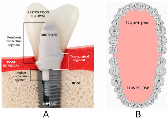
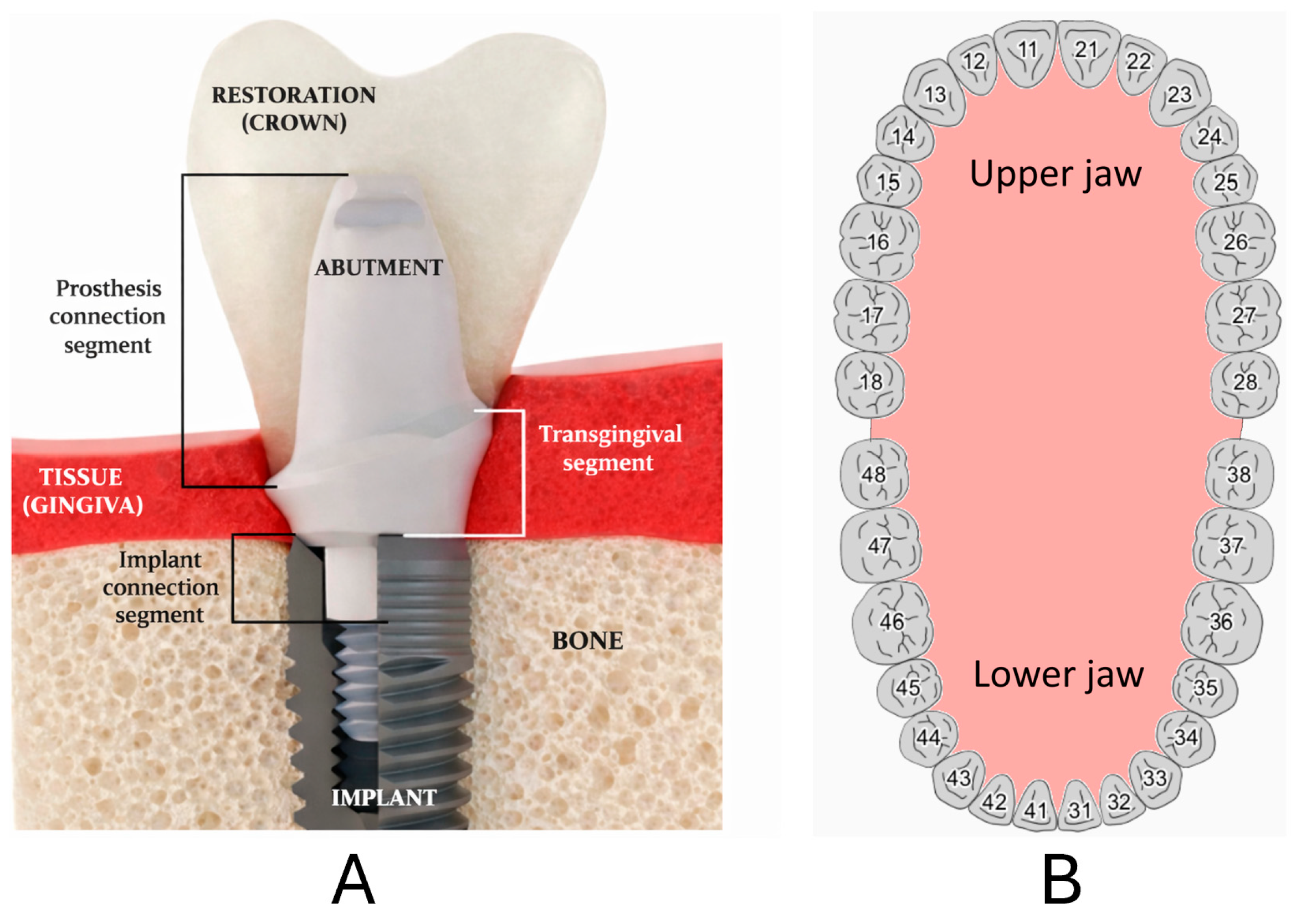
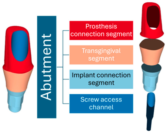
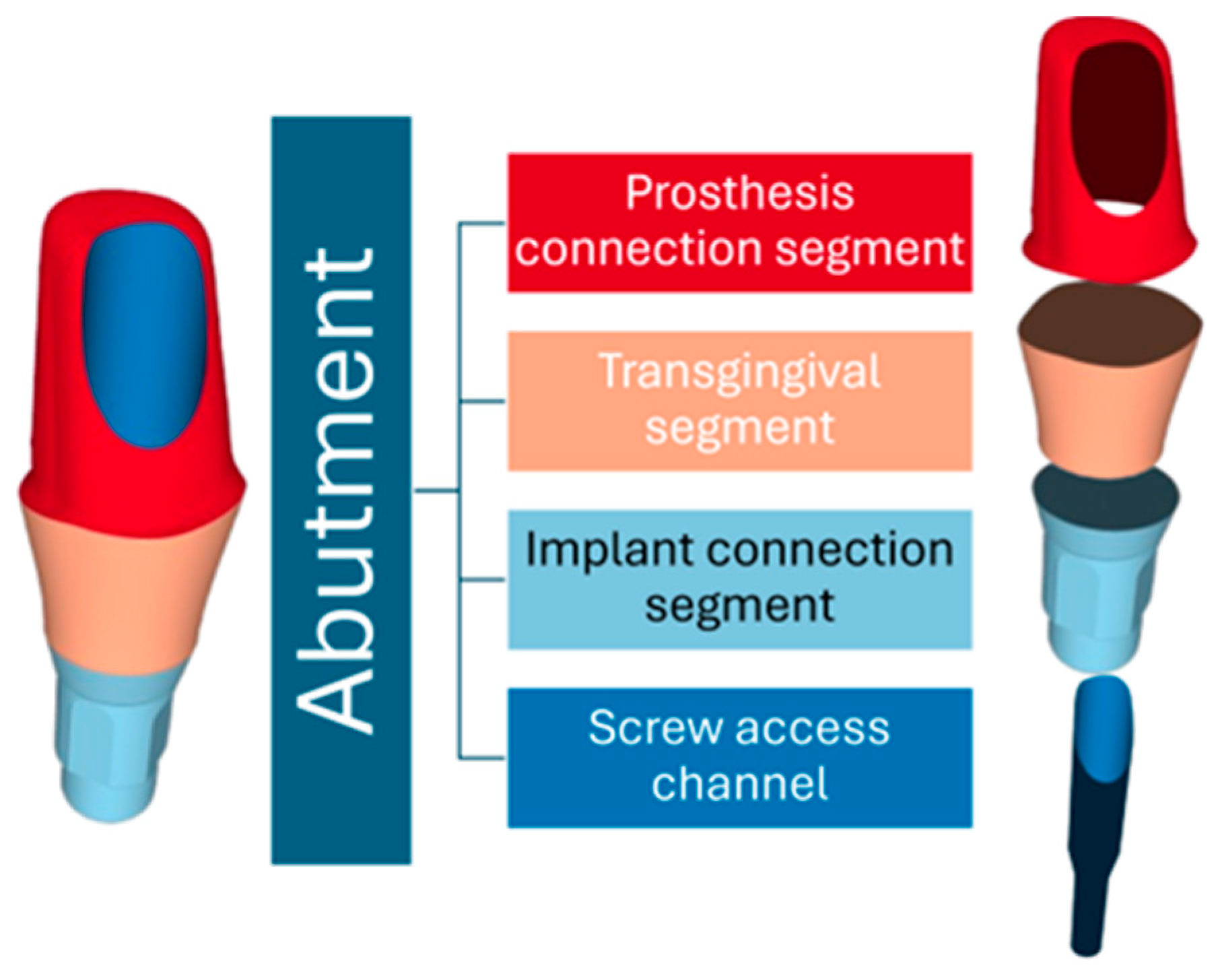
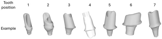
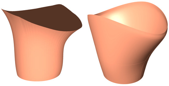
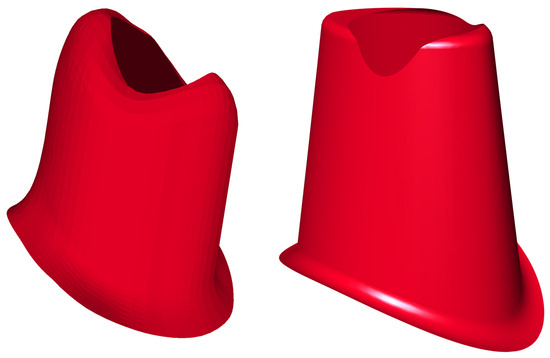
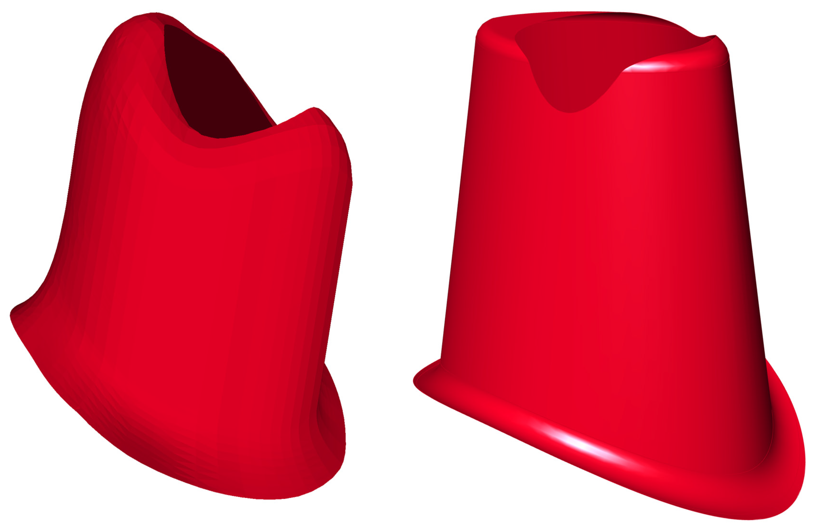
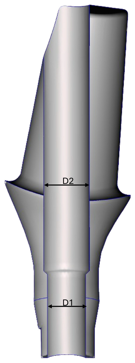
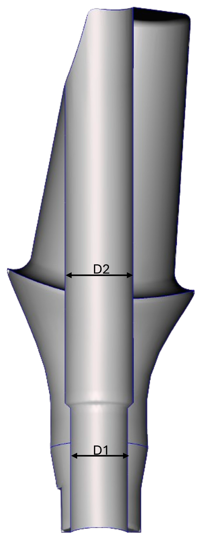
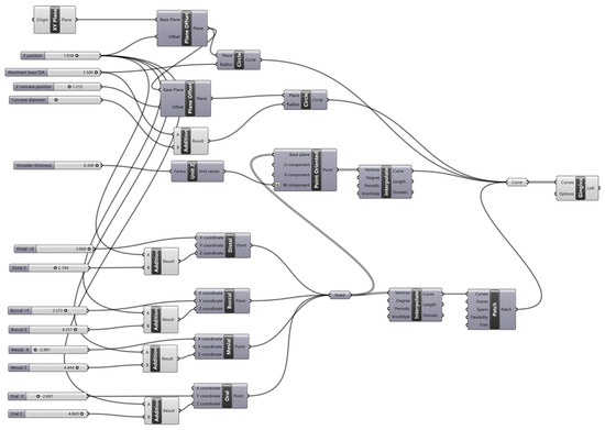
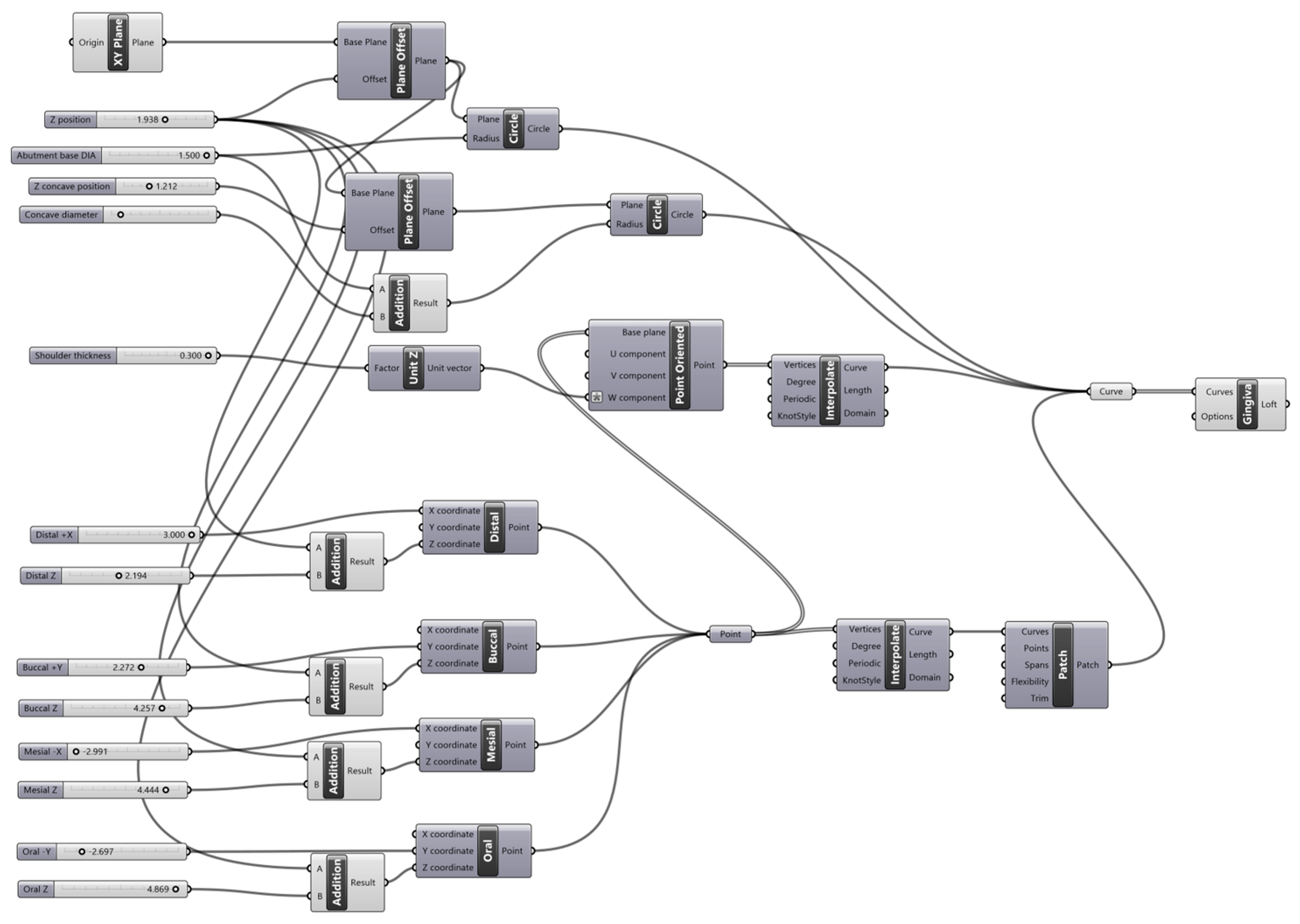
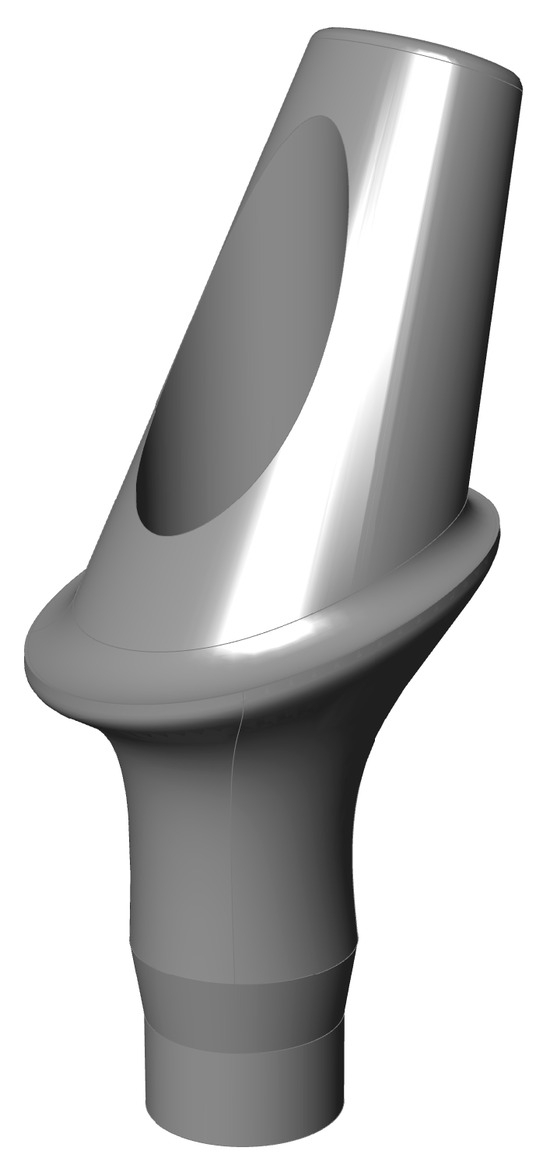
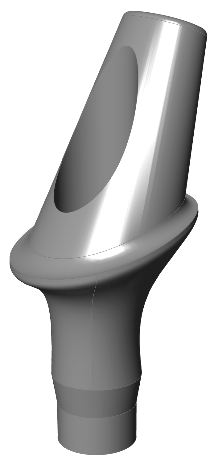
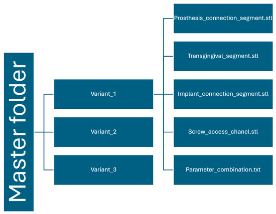
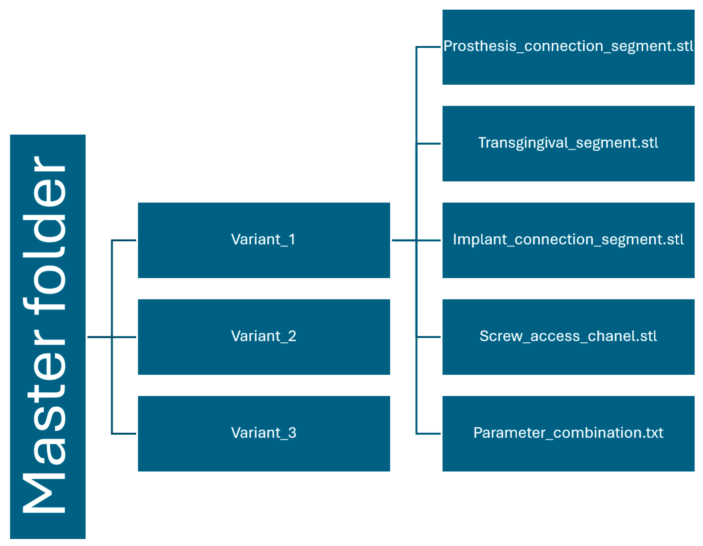
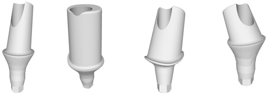
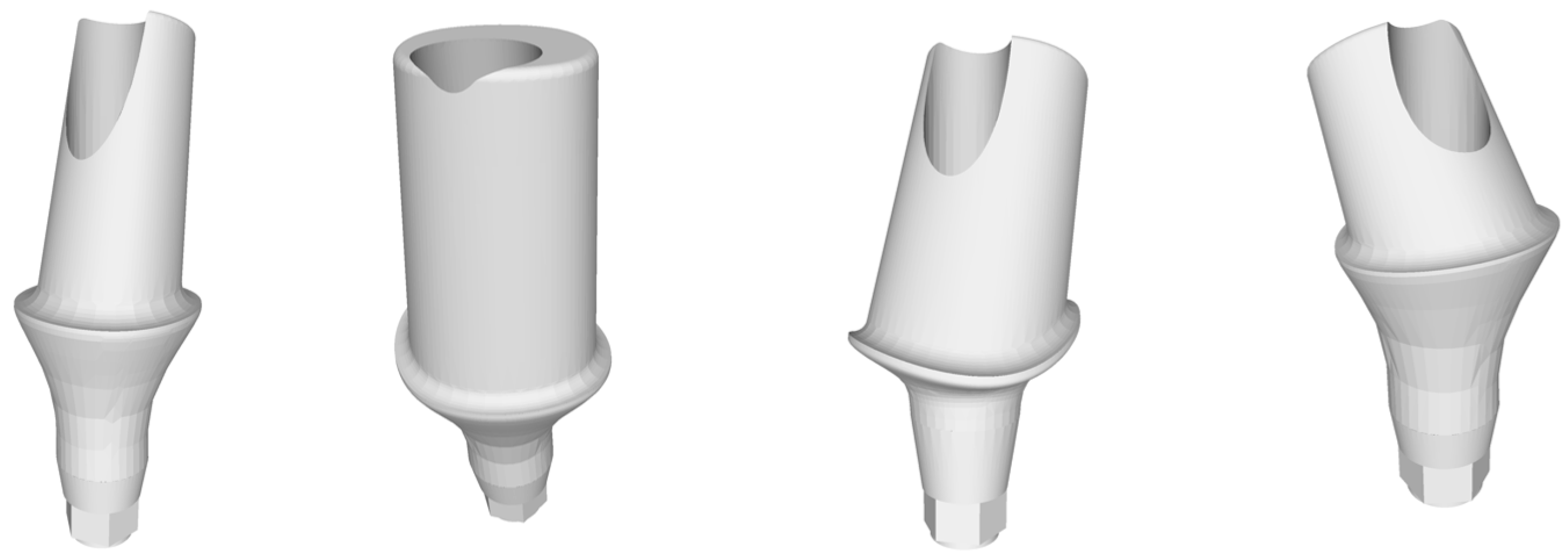
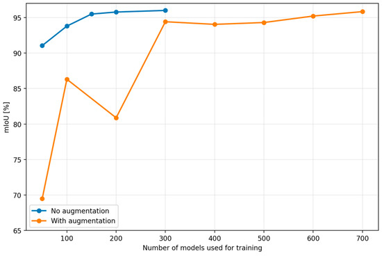
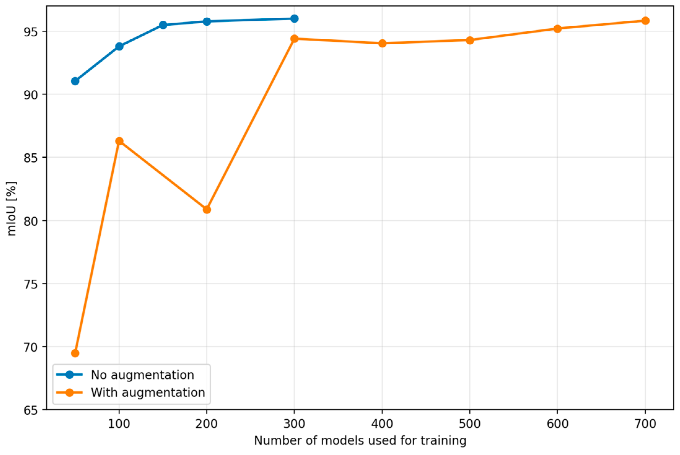
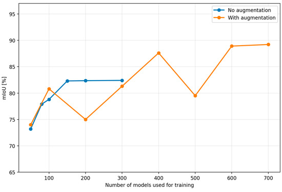
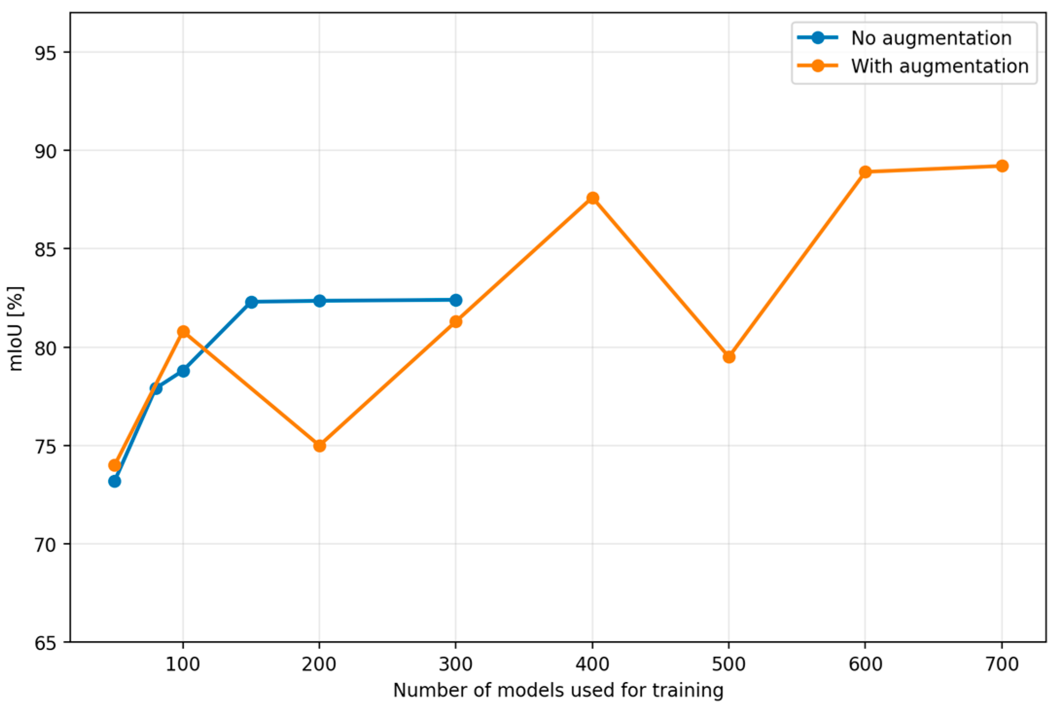
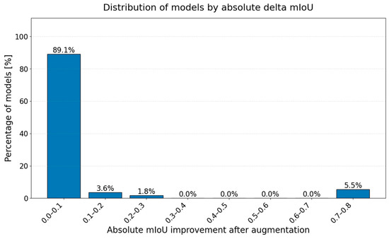
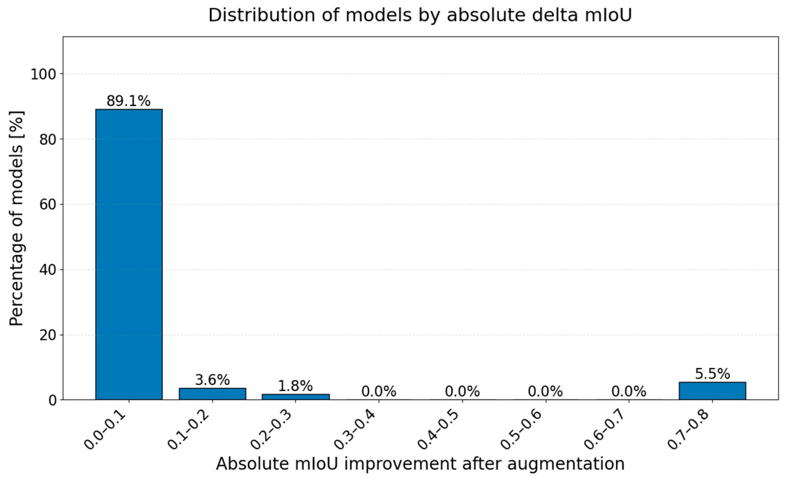
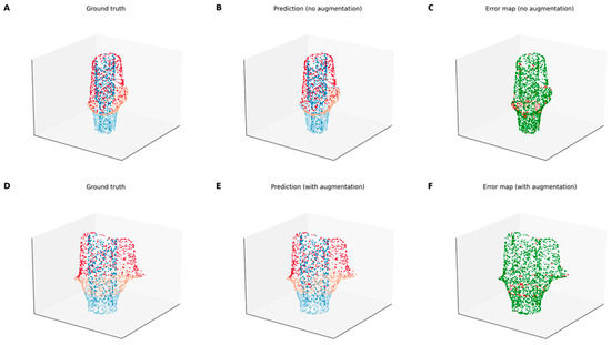
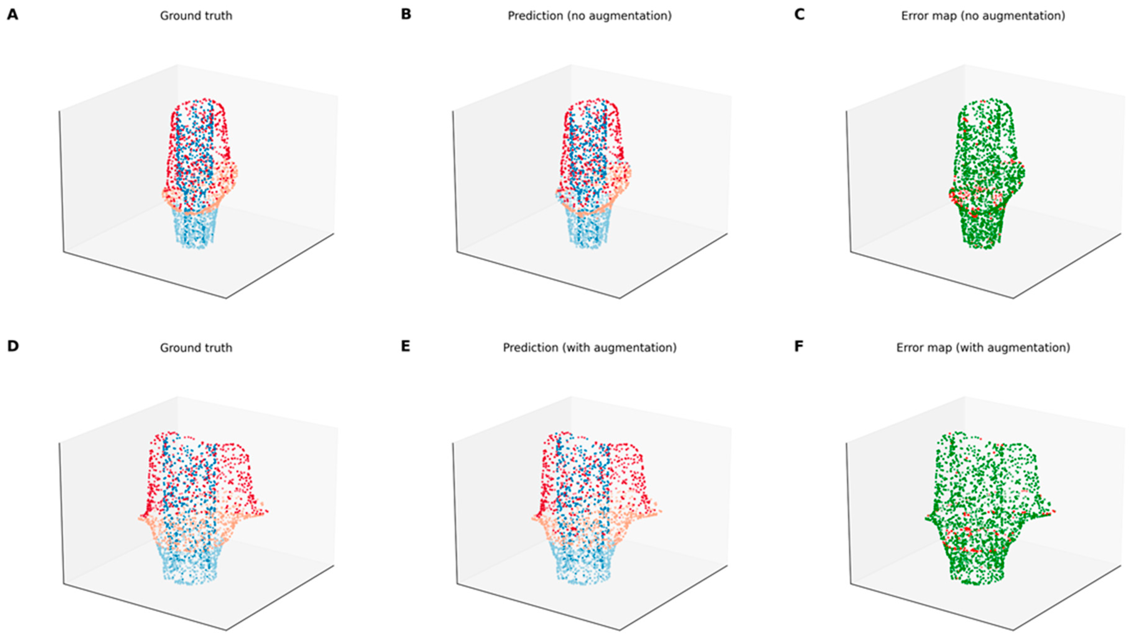
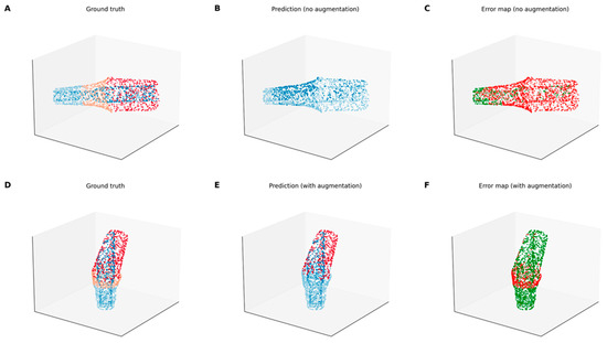
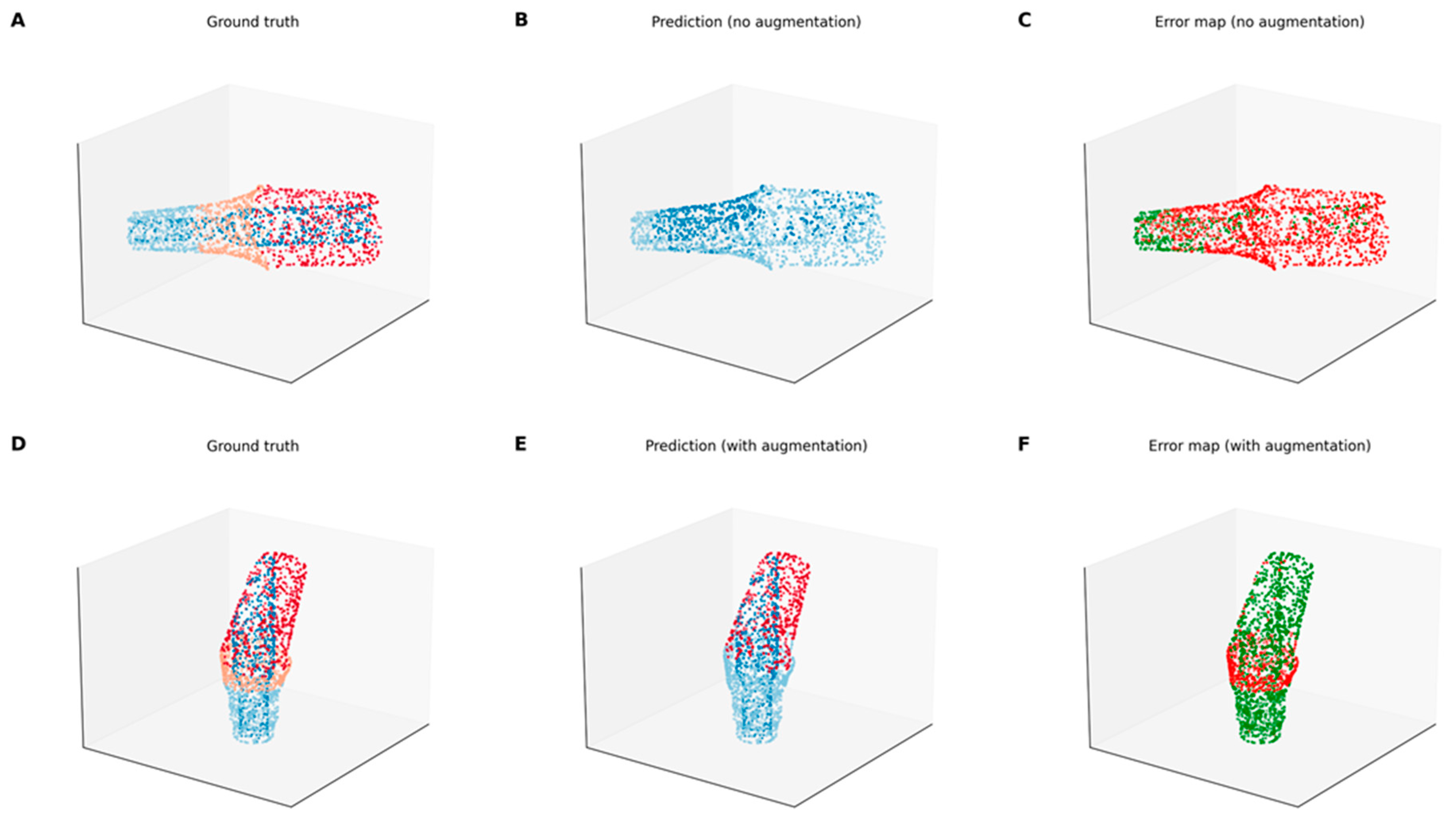
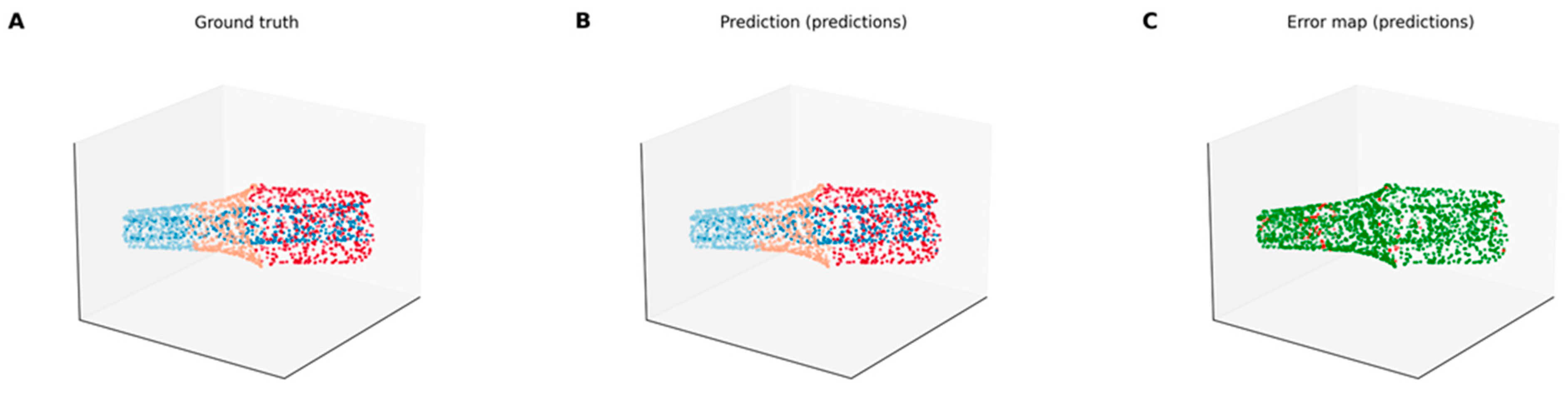

Disclaimer/Publisher’s Note: The statements, opinions and data contained in all publications are solely those of the individual author(s) and contributor(s) and not of MDPI and/or the editor(s). MDPI and/or the editor(s) disclaim responsibility for any injury to people or property resulting from any ideas, methods, instructions or products referred to in the content. |
© 2026 by the authors. Licensee MDPI, Basel, Switzerland. This article is an open access article distributed under the terms and conditions of the Creative Commons Attribution (CC BY) license.