


Abstract
Unsupervised topic extraction is a vital step in automatically extracting concise contentual information from large text corpora. Existing topic extraction methods lack the capability of linking relations between these topics which would further help text understanding. Therefore we propose utilizing the Decomposition into Directional Components (DEDICOM) algorithm which provides a uniquely interpretable matrix factorization for symmetric and asymmetric square matrices and tensors. We constrain DEDICOM to row-stochasticity and non-negativity in order to factorize pointwise mutual information matrices and tensors of text corpora. We identify latent topic clusters and their relations within the vocabulary and simultaneously learn interpretable word embeddings. Further, we introduce multiple methods based on alternating gradient descent to efficiently train constrained DEDICOM algorithms. We evaluate the qualitative topic modeling and word embedding performance of our proposed methods on several datasets, including a novel New York Times news dataset, and demonstrate how the DEDICOM algorithm provides deeper text analysis than competing matrix factorization approaches.
1. Introduction
Matrix factorization methods have always been a staple in many natural language processing (NLP) tasks. Factorizing a matrix of word co-occurrences can create both low-dimensional representations of the vocabulary, so-called word embeddings [1,2], that carry semantic and topical meaning within them, as well as representations of meaning that go beyond single words to latent topics.
Decomposition into Directional Components (DEDICOM) is a matrix factorization technique that factorizes a square, possibly asymmetric, matrix of relationships between items into a loading matrix of low-dimensional representations of each item and an affinity matrix describing the relationships between the dimensions of the latent representation (see Figure 1 for an illustration).
Figure 1.
(a) The DEDICOM algorithm factorizes a square matrix
into a loading matrix
and an affinity matrix
(b) The tensor DEDICOM algorithm factorizes a three dimensional tensor
into a loading matrix
and a three dimensional affinity tensor
We introduce a modified row-stochastic variation of DEDICOM, which allows for interpretable loading vectors and apply it to different matrices of word co-occurrence statistics created from Wikipedia based semi-artificial text documents. Our algorithm produces low-dimensional word embeddings, where one can interpret each latent factor as a topic that clusters words into meaningful categories. Hence, we show that row-stochastic DEDICOM successfully combines the task of learning interpretable word embeddings and extracting representative topics.
We further derive a similar model for factorization of three-dimensional data tensors, which represent word co-occurrence statistics for text corpora with intrinsic structure that allows for some separation of the corpus into subsets (e.g., a news corpus structered by time).
An interesting aspect of this type of factorization is the interpretability of the affinity matrix. An entry in the matrix directly describes the relationship between the topics of the respective row and column and one can therefore use this tool to extract topics that a certain text corpus deals with and analyze how these topics are connected in the given text.
In this work we first describe the aforementioned DEDICOM algorithm and provide details on the modified row-stochasticity constraint and on optimization. We further expand our model to factorize three-dimensional tensors and introduce a multiplicative update rule that facilitates the training procedure. We then present results of various experiments on both semi-artificial text documents (combinations of Wikipedia articles) and real text documents (movie reviews and news articles) that show how our approach is able to capture hidden latent topics within text corpora, cluster words in a meaningful way and find relationships between these topics within the documents.
This paper is an extension of previous work [3]. In addition to the algorithms and experiments described there, we here add the extension of the DEDICOM algorithm to three-dimensional tensors, introduce a multiplicative update rule to increase training stability and present new experiments on two additional text corpora (Amazon reviews and New York Times news articles).
2. Related Work
Matrix factorization describes the task of compressing the most relevant information from a high-dimensional input matrix into multiple low-dimensional factor matrices, with either approximate or exact input reconstruction (see for example [4] for a theoretical overview of common methods and their applications). In this work we consider the DEDICOM algorithm, which has a long history of providing an interpretable matrix or tensor factorization, mostly for rather low-dimensional tasks.
First described in [5], it since has been applied to analysis of social networks [6], email correspondence [7] and video game player behavior [8,9]. DEDICOM also has successfully been employed to NLP tasks such as part of speech tagging [10], however to the best of our knowledge we provide the first implementation of DEDICOM for simultaneous word embedding learning and topic modeling.
Many works deal with the task of putting constraints on the factor matrices of the DEDICOM algorithm. In [7,8], the authors constrain the affinity matrix R to be non-negative, which aids interpretability and improves convergence behavior if the matrix to be factorized is non-negative. However, their approach relies on the Kronecker product between matrices in the update step, solving a linear system of , where n denotes the number of items in the input matrix and k the number of latent factors. These dimensions make the application on text data, where n describes the number of words in the vocabulary, a computationally futile task. Constraints on the loading matrix, A, include non-negativity as well (see [7]) or column-orthogonality as in [8].
In contrast, we propose a new modified row-stochasticity constraint on A, which is tailored to generate interpretable word embeddings that carry semantic meaning and represent a probability distribution over latent topics.
The DEDICOM algorithm has previously been applied to tensor data as well, for example in [11], in which the authors apply the algorithm on general multirelational data by computing an exact solution for the affinity matrix. Both [6,7] explore a slight variation of our tensor DEDICOM approach to analyze relations in email data and [12] apply a similar model on non-square input tensors.
Previous matrix factorization based methods in the NLP context mostly dealt with either word embedding learning or topic modeling, but not with both tasks combined.
For word embeddings, the GloVe [2] model factorizes an adjusted co-occurrence matrix into two matrices of the same dimension. The work is based on a large text corpus with a vocabulary of 400,000 and produces word embeddings of dimension . In order to maximize performance on the word analogy task, the authors adjusted the co-occurrence matrix to the logarithmized co-occurrence matrix and added bias terms to the optimization objective.
A model conceived around the same time, word2vec [13], calculates word embeddings not from a co-occurrence matrix but directly from the text corpus using the skip-gram or continuous-bag-of-words approach. More recent work [1] has shown that this construction is equivalent to matrix factorization on the pointwise mutual information (PMI) matrix of the text corpus, which makes it very similar to the glove model described above.
Both models achieve impressive results on word embedding related tasks like word analogy, however the large dimensionality of the word embeddings makes interpreting the latent factors of the embeddings impossible.
On the topic modeling side, matrix factorization methods are routinely applied as well. Popular algorithms like non-negative matrix factorization (NMF) [14], singular value decomposition (SVD) [15,16] and principal component analysis (PCA) [17] compete against the probabilistic latent dirichlet allocation (LDA) [18] to cluster the vocabulary of a word co-occurrence or document-term matrix into latent topics. (More recent expansions of these methods can be found in [19,20].) Yet, we empirically show that the implicitly learned word embeddings of these methods lack semantic meaning in terms of the cosine similarity measure.
We benchmark our approach qualitatively against these methods in Section 4.3 and the Appendix A and Appendix B.
3. Constrained DEDICOM Models
In this section we provide a detailed theoretical view at different constrained DEDICOM algorithms utilized for factorizing word co-occurrence based positive pointwise mutual information matrices and tensors.
We first consider the case of a two-dimensional input matrix S (see Figure 1a) in Section 3.1. We then present an extension of the algorithm for three-dimension input tensors S (see Figure 1b) in Section 3.2. Finally we derive a multiplicative update rule for non-negative tensor DEDICOM.
3.1. The Row-Stochastic DEDICOM Model for Matrices
For a given language corpus consisting of n unique words we calculate a co-occurrence matrix by iterating over the corpus on a word token level with a sliding context window of specified size. Then
Note that the word context window can be applied symmetrically or asymmetrically around each word. We choose a symmetric context window, which implies a symmetric co-occurrence matrix, .
We then transform the co-occurrence matrix into the pointwise mutual information matrix (PMI), which normalizes the counts in order to extract meaningful co-occurrences from the matrix. Co-occurrences of words that occur regularly in the corpus are decreased since their appearance together might be nothing more than a statistical phenomenon, the co-occurrence of words that appear less often in the corpus give us meaningful information about the relations between words and topics. We define the PMI matrix as
where is the sum of all co-occurrence counts of W, the row sum and the column sum.
Since the co-occurrence matrix W is symmetrical, the transformed PMI matrix is symmetrical as well. Nevertheless, DEDICOM is able to factorize both symmetrical and non-symmetrical matrices. We expand details on symmetrical and non-symmetrical relationships in Section 3.4.
Additionally, we want all entries of the matrix to be non-negative, our final matrix to be factorized is therefore the positive PMI (PPMI)
Our aim is to decompose this matrix using row-stochastic DEDICOM as
where , , denotes the transpose of A and . Literature often refers to A as the loading matrix and R as the affinity matrix. A gives us for each word i in the vocabulary a vector of size k, the number of latent topics we wish to extract. The square matrix R then provides possibility for interpretation of the relationships between these topics.
Empirical evidence has shown that the algorithm tends to favor columns unevenly, such that a single column receives a lot more weight in its entries than the other columns. We try to balance this behavior by applying a column-wise z-normalization on A, such that all columns have zero mean and unit variance.
In order to aid interpretability we wish each word embedding to be a distribution over all latent topics, i.e., entry in the word-embedding matrix provides information on how much topic b describes word i.
To implement these constraints we therefore apply a row-wise softmax operation over the column-wise z-normalized A matrix by defining as
and optimizing A for the objective
Note that after applying the row-wise softmax operation all entries of are non-negative.
To judge the quality of the approximation (6) we apply the Frobenius norm, which measures the difference between S and . The final loss function we optimize our model for is therefore given by
with
and defined in (5).
To optimize the loss function we train both matrices using alternating gradient descent similar to [8]. Within each optimization step we apply
with being individual learning rates for both matrices and representing an arbitrary gradient based update rule with additional hyperparameters . For our experiments we employ automatic differentiation methods. For details on the implementation of the algorithm above refer to Section 4.2.
3.2. The Constrained DEDICOM Model for Tensors
In this section we extend the model described above to three-dimensional tensors as input data. As above, the input describes the co-occurrences of vocabulary items in a text corpus. However, we consider additionally structured text: Instead of one matrix describing the entire corpus we unite multiple matrices of co-occurrences into one tensor . Each of the t slices then consists of an adjusted PPMI matrix for a subset of the text corpus. This structure could originate for instance from different data (e.g., different Wikipedia articles), different topical subsets of the data source (e.g., reviews for different articles) or describe time-slices (e.g., news articles for certain time periods).
To construct the PPMI tensor we again take a vocabulary over the entire corpus. For each subset l we then calculate a co-occurrence matrix as described above. Stacking these matrices yields the co-occurrence tensor .
When transforming slice into a PMI matrix we want to apply information from the entire corpus. We therefore do not only calculate the column, the row and the total sums on the corresponding subset but on the entire text corpus. Therefore
where is the sum of all co-occurrence counts of , the row sum and the column sum.
Finally we define the positive pointwise mutual information tensor as
We decompose this input tensor into a matrix and a tensor , such that
where we multiply each slice of
with A and to reconstruct the corresponding slice of :
We keep our naming convention for A as the loading matrix and as the affinity tensor, since again A gives us for each word i in the vocabulary a vector of size k and for each slice l the square matrix provides information on the relationships between the topics in the l-th input slice.
Note that in this framework, the DEDICOM algorithm described in the previous section is equivalent to tensor DEDICOM with .
Update steps can then be taken via alternating gradient descent on A and . As in the previous section, one can now add additional constraints to A and and calculate the gradients as in (10), using automatic differentiation methods. Taking update steps of size and respectively leads to an eventual convergence to some local or global minimum of the loss (16) with respect to the original or constrained A and
.
Alternatively, constraints can be added to A and
by methods like projected gradient descent and the Frank-Wolfe algorithm [21] which either adjust the respective matrix or tensor to be constrained after the gradient step or apply the general gradient step such that the matrix or tensor never leaves the constrained area.
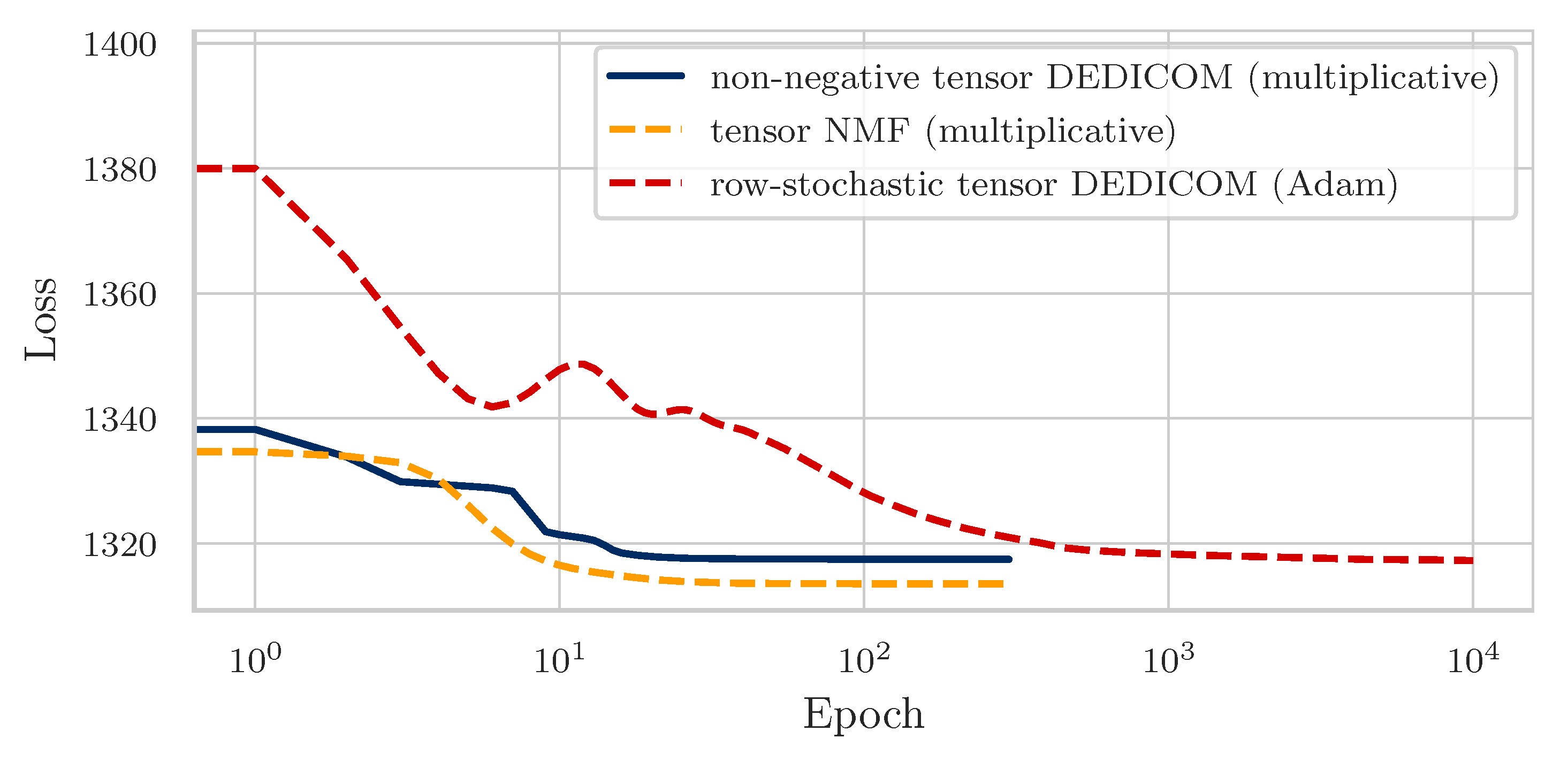
However, empirical results show that automatic differentiation methods lead to slow and unstable training convergence and worse qualitative results when applying the mentioned constraints on the factor matrices and tensors. We therefore derive an alternative method of applying alternating gradient descent to A and
based on multiplicative update rules. This does not only improve training stability and convergence behavior but also lead to better qualitative results (see Section 4.3 and Figure 2).
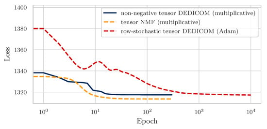
Figure 2.
Reconstruction loss development during tensor factorization training. The x-axis plots the number of epochs on a logarithmic scale, the y-axis plots the corresponding reconstruction error for each method.
We derive the gradients for A and R analytically and set the learning rates and individually for each element as for matrix A and for each element as for tensor , such that the resulting update step is an element-wise multiplication of the respective matrix or tensor.
We derive the updates for the matrix algorithm first and later extend them for the tensor case. For detailed derivations refer to Appendix B. For A we derive the gradient analytically as
Therefore the update step is
For R we derive the gradient analytically as
Therefore the update step is
Since for all , in both (23) and (27) each element of the multiplier matrix is positive if both and in all entries. Therefore, initializing both matrices with positive values results in an update step that keeps the elements of A and R positive.
To extend this rule to tensor DEDICOM, consider that the analytical derivatives hold for
and A by considering each slice and individually:
For A we set as
Then the update step is
3.3. On Symmetry
The DEDICOM algorithm is able to factorize both symmetrical and asymmetrical matrices S. For a given matrix A, the symmetry of R dictates the symmetry of the product , since
if for all . We therefore expect a symmetric matrix S to be decomposed into with a symmetric R, which is confirmed by our experiments. Factorizing a non-symmetric matrix leads to a non-symmetric R, the asymmetric relation between items leads to asymmetric relations between the latent factors. The same relations hold for each slice and in tensor DEDICOM.
3.4. On Interpretability
We have
i.e., we can estimate the probability of co-occurrence of two words and from the word embeddings and and the matrix R, where denotes the i-th row of A.
If we want to predict the co-occurrence between words and we consider the latent topics that make up the word embeddings and , and sum up each component from with each component with respect to the relationship weights given in R.
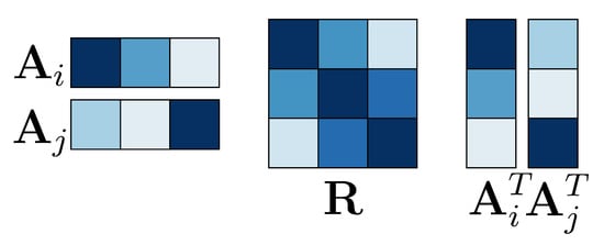
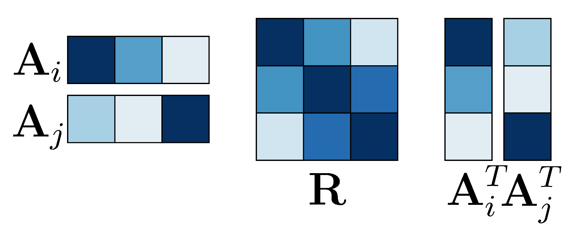
Two words are likely to have a high co-occurrence if their word embeddings have larger weights in topics that are positively connected by the R matrix. Likewise a negative entry makes it less likely for words with high weight in the topics b and c to occur in the same context. See Figure 3 for an illustrated example.
Figure 3.
The affinity matrix R describes the relationships between the latent factors. Illustrated here are two word embeddings, corresponding to the words and . Darker shades represent larger values. In this example we predict a large co-occurrence at and because of the large weight on the diagonal of the R matrix. We predict a low co-occurrence at and since the large weights on and interact with low weights on and .
Having an interpretable embedding model provides value beyond analysis of the affinity matrix of a single document. The worth of word embeddings is generally measured in their usefulness for downstream tasks. Given a prediction model based on word embeddings as one of the inputs, further analysis of the model behavior is facilitated when latent input dimensions easily translate to semantic meaning.
In most word embedding models, the embedding vector of a single word is not particularly useful in itself. The information only lies in its relationship (i.e., closeness or cosine similarity) to other embedding vectors. For example, an analysis of the change of word embeddings and therefore the change of word meaning within a document corpus (for example a news article corpus) can only show how various words form different clusters or drift apart over time. Interpretabilty of latent dimensions would provide tools to also consider the development of single words within the given topics.
All considerations above hold for the three-dimensional tensor case, in which we analyze a slice together with the common word embedding matrix A to gain insight into the input data slice .
4. Experiments and Results
In the following section we describe our experimental setup in full detail (Our Python implementation to reproduce the results is available on https://github.com/LarsHill/text-dedicom-paper. Additionally, we provide a snapshot of our versions of the applied public datasets (Wikipedia articles and Amazon reviews). ) and present our results on the simultaneous topic (relation) extraction and word embedding learning task. We compare these results against competing matrix and tensor factorization methods for topic modeling, namely NMF (including a Tucker-2 variation compatible with tensors), LDA and SVD.
4.1. Data
We conducted our experiments on three orthogonal text datasets which cover different text domains and allow for a thorough empirical analysis of our proposed methods.
The first corpus leveraged triplets of individual Wikipedia articles. The articles were retrieved as raw text via the official Wikipedia API using the wikipedia-api library. We differentiated between thematically similar (e.g., “Dolphin” and “Whale”) and thematically different articles (e.g., “Soccer” and “Donald Trump”). Each article triplet was categorized into one of three classes: All underlying Wikipedia articles were thematically different, two articles were thematically similar and one was different, and all articles were thematically similar. The previous paper [3] contained an extensive evaluation over 12 triples of articles in the supplementary material. In this work we focused on the three triples described in the previous main paper, namely
- “Soccer”, “Bee”, “Johnny Depp”,
- “Dolphin”, “Shark”, “Whale”, and
- “Soccer”, “Tennis”, “Rugby”.
Depending on whether the article triplets were represented as input matrix or tensor they were processed differently. In the case of a matrix input all three articles got concatenated to form a new artificially generated document. In the case of a tensor input the articles remained individual documents later which later represented slices in the tensor representation.
To analyze the topic extraction capability of constrained DEDICOM also on text which was rather prone to grammatical and syntactical errors, we utilized a subset of the Amazon review dataset [22]. In particular, we restricted ourselves to the “movie” product category and created a corpus consisting of six text documents holding the concatenated reviews from the following films respectively, “Toy Story 1”, “Toy Story 3”, “Frozen”, “Monsters, Inc.”, “Kung Fu Panda” and “Kung Fu Panda 2”. Grouping the reviews by movie affiliation enabled us to generate a tensor representation of the corpus which we factorized via non-negative tensor DEDICOM to analyze topic relations across movies. Table 1 lists the number of reviews per movie and shows that based on review count “Kung Fu Panda 1” was the most popular among the six films.
Table 1.
Amazon movie review corpus grouped by movie and number of reviews per slice of input tensor.
The third corpus represented a complete collection of New York Times news articles ranging from 1st September 2019 to 31st August 2020. The articles were taken from the New York Times website and covered a wide range of sections (see Table 2).
Table 2.
New York Times news corpus composition by section and number of articles.
Instead of grouping the articles by section we binned and concatenated them by month yielding 12 news documents containing monthly information (see Table 3 for details on the article count per month). Thereby, the factorization of tensor DEDICOM allowed for an analysis of topic relations and their changes over time.
Table 3.
New York Times news corpus grouped by month and number of articles. This corresponds to the number of articles per slice of input tensor.
Before transforming the text documents to matrix or tensor representations we applied the following textual preprocessing steps. First, the whole text was made lower-cased. Second, we tokenized the text making use of the word-tokenizer from the nltk library and removed common English stop words, including contractions such as “you’re” and “we’ll”. Lastly we cleared the text from all remaining punctuation and deleted digits, single characters and multi-spaces (see Table 4 for an overview of corpora statistics after preprocessing).
Table 4.
Overview of word count statistics after preprocessing for all datasets. Columns represent from left to right the total number of words per corpus, total number of unique words per corpus, average number of total words per article, average number of unique words per article and the cutoff frequency of the 10,000th most common word. Wikipedia article combinations: Dolphin, Shark, Whale (DSW), Soccer, Bee, Johnny Depp (SBJ), Soccer, Tennis, Rugby (STR).
Next, we utilized all preprocessed documents in a corpus to extract a fixed size vocabulary of n = 10,000 most frequent tokens. Since our dense input tensor was of dimensionality , a larger vocabulary size led to a significant increase in memory consumption. Based on the total number of unique corpora words reported in Table 4, a maximum vocabulary size of n = 10,000 was reasonable for the three Wikipedia corpora and the Amazon reviews corpus. Only the New York Times dataset could potentially have benefited from a larger vocabulary size.
Based on this vocabulary a symmetric word co-occurrence matrix was calculated for each of the corpus documents. When generating the matrix we only considered context words within a symmetrical window around the base word. Analysis in [2,3] showed that the window size in the range of 6 to 10 had little impact on performance. Thus, following our implementation in [3], we chose a window size of 7, the default in the original glove implementation. Like in [2], each context word only contributed to the total word pair count, given it was d words apart from the base word. To avoid any bias or prior information from the structure and order of the concatenated Wikipedia articles, reviews or news articles, we randomly shuffled the vocabulary before creating the co-occurrence matrix. As described in Section 3 we then transformed the co-occurrence matrix to a positive PMI matrix. If the corpus consisted of just one document the generated PPMI matrix functions as input for the row-stochastic DEDICOM algorithm. If the corpus consisted of several documents (e.g., one news document per month) the individual PPMI matrices were stacked to a tensor which in turn represented the input for the non-negative tensor DEDICOM algorithm.
The next section sheds light upon the training process of row-stochastic DEDICOM, non-negative tensor DEDICOM and the above mentioned competing matrix and tensor factorization methods, which will be benchmarked against our results in Section 4.3 and in the Appendix A and Appendix B.
4.2. Training
As thoroughly outlined in Section 3 we trained both the row-stochastic DEDICOM and non-negative tensor DEDICOM with the alternating gradient descent paradigm.
In the case of a matrix input and a row-stochasticity constraint on A we utilize automatic differentiation from the PyTorch library to perform update steps on A and R. First, we initialized the factor matrices and , by randomly sampling all elements from a uniform distribution centered around 1, . Note that after applying the softmax operation on A all rows of A were stochastic. Therefore, scaling R by
would result in the initial decomposition yielding reconstructed elements in the range of , the element mean of the PPMI matrix S, and thus, speeding up convergence. Second, A and R were iteratively updated employing the Adam optimizer [23] with constant individual learning rates of and and hyperparameters , and . Both learning rates were identified through an exhaustive grid search. We trained for = 15,000 until convergence, where each epoch consisted of an alternating gradient update with respect to A and R.
Algorithm 1 illustrates the just described training procedure.
| Algorithm 1 The row-stochastic DEDICOM algorithm | |
| 1: initialize | ⊳See Equation (40) for the definition of |
| 2: initialize , , | ⊳Adam algorithm hyperparameters |
| 3: initialize , | ⊳Individual learning rates |
| 4: for i in , num_epochs do | |
| 5: Calculate loss | ⊳See Equation (7) |
| 6: | |
| 7: | |
| 8: return and R, where | ⊳See Equation (5) |
In the case of a tensor input and an additional non-negativity constraint on
we noticed an inferior training performance with automatic differentiation methods. Hence, due to faster and more stable training convergence and improved qualitative results, we updated A and iteratively via derived multiplicative update rules enforcing non-negativity. Again, we initialized and , by randomly sampling all elements from a uniform distribution centered around 1, . In order to ensure that the initialized components yielded a reconstructed tensor whose elements were in the same range of the input, we calculated an appropriate scaling factor for each tensor slice as
Next, we scaled A by and each slice by before starting the alternating multiplicative update steps for . The detailed derivation of the update rules is found in Section 3.2 and their iterative application in the training process is described in Algorithm 2.
We implemented NMF, LDA and SVD using the sklearn library. In all cases the learnable factor matrices were initialized randomly and default hyperparameters were applied during training. For NMF the multiplicative update rule from [14] was utilized.
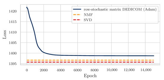
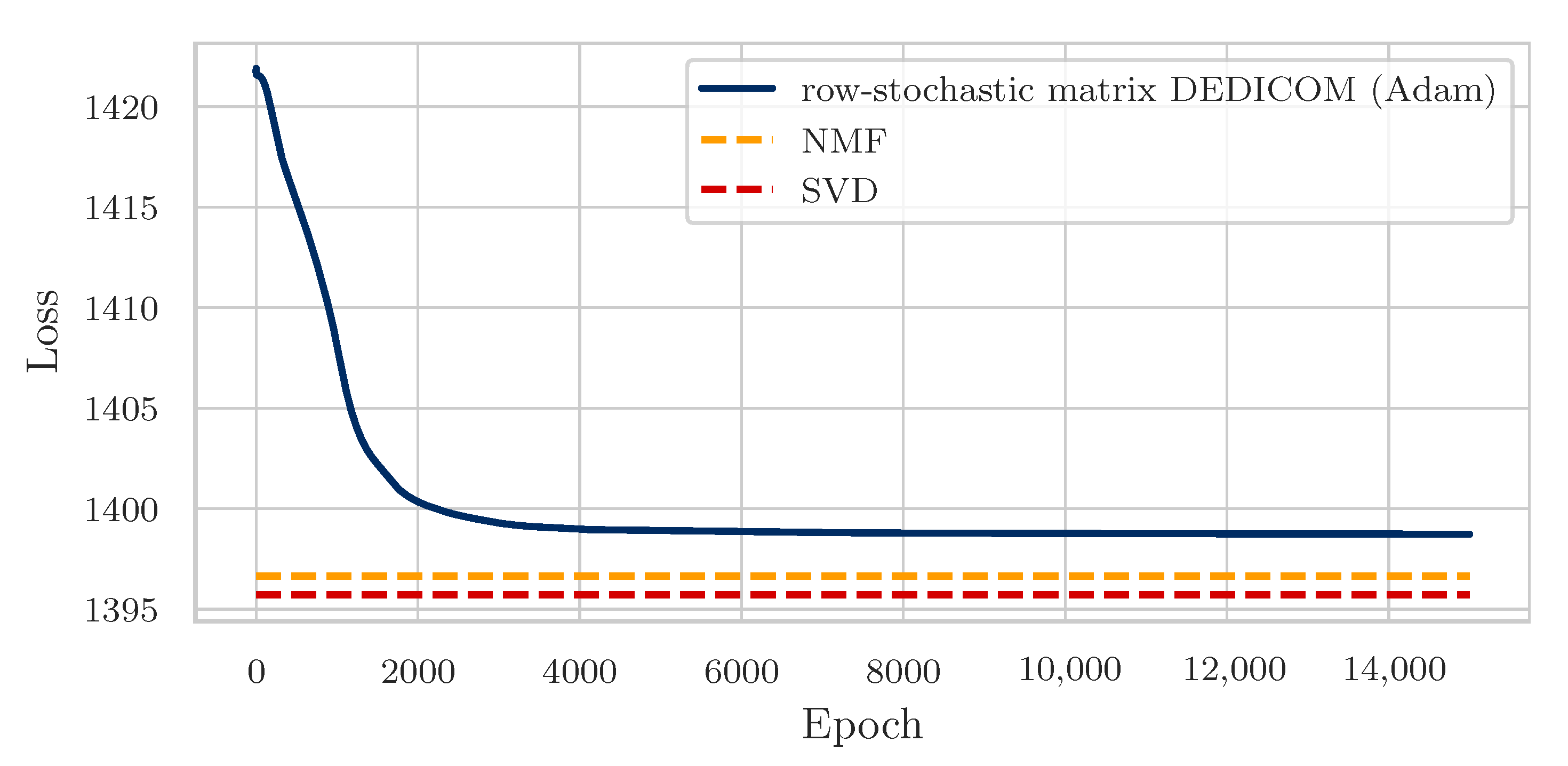
Figure 4 shows the convergence behavior of the row-stochastic matrix DEDICOM training process and the final loss of NMF and SVD. Note that LDA optimized a different loss function, which is why the calculated loss was not comparable and therefore excluded. We see that the final loss of DEDICOM was located just above the other losses, which is reasonable when considering the row stochasticity contraint on A and the reduced parameter amount of compared to NMF () and SVD ().
Figure 4.
Reconstruction loss development during matrix factorization training. The x-axis plots the number of epochs, the y-axis plots the corresponding reconstruction error for each method.
To also have a benchmark model for our constrained tensor DEDICOM methods to compare against, we implemented a Tucker-2 variation of NMF, named tensor NMF (TNMF), which factorized the input tensor
as
Its training procedure closely followed the above described alternating gradient descent approach for non-negative tensor DEDICOM. However, due to the two-way factorization (three-way for DEDICOM) the scaling factor to properly initialize
and H had to be adapted to
Analogous to Figure 4, we compared the training stability and convergence speed of our implemented tensor factorization methods. In particular, Figure 2 visualizes the reconstruction loss development for non-negative tensor DEDICOM trained via multiplicative update rules, row-stochastic tensor DEDICOM trained with automatic differentiation and the Adam optimizer and tensor NMF. It could be clearly observed that row-stochastic tensor DEDICOM converged much slower than the other two models trained with multiplicative update rules (learning rates were implicit here and did not have to be tuned).
4.3. Results
In the following, we present our results of training the above mentioned constrained DEDICOM factorizations on different text corpora to simultaneously learn interpretable word embeddings and meaningful topic clusters and their relations.
First, we focused our analysis on row-stochastic matrix DEDICOM applied to the synthetic Wikipedia text documents described in Section 4.1. For compactness reasons we primarily considered the document “Soccer, Bee and Johnny Depp”, set the number of topics to and refer to Appendix A.1 for the other article combinations and competing matrix factorization results. Second, we extended our evaluation to the tensor representation of the Wikipedia documents (, one article per tensor slice) and compared the performance of non-negative (multiplicative updates) and row-stochastic (Adam updates) tensor DEDICOM. Lastly, we applied non-negative tensor DEDICOM to the binned Amazon movie and New York Times news corpora to investigate topic relations across movies and over time. We again point the interested reader to Appendix A for additional results and the comparison to tensor NMF.
In the first step, we evaluated the quality of the learned latent topics by assigning each word embedding to the latent topic dimension that represents the maximum value in , e.g.,
and thus, was matched to Topic 5. Next, we decreasingly sorted the words within each topic based on their matched topic probability. Table 5 shows the overall number of allocated words and the resulting top 10 words per topic together with each matched probability.
Table 5.
The top 10 representative words per dimension of the basis matrix , trained on the Wikipedia data as input matrix using automatic gradient methods.
Indicated by the high assignment probabilities, one can see that columns 1, 2, 4, 5 and 6 represent distinct topics, which can easily be interpreted. Topic 1 and 4 were related to soccer, where 1 focused on the game mechanics and 4 on the organizational and professional aspect of the game. Topic 2 and 6 clearly referred to Johnny Depp, where 2 focused on his acting career and 6 on his difficult relationship to Amber Heard. The fifth topic obviously related to the insect “bee”. In contrast, Topic 3 did not allow for any interpretation and all assignment probabilities were significantly lower than for the other topics.
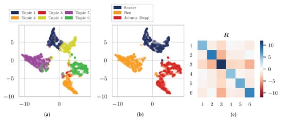
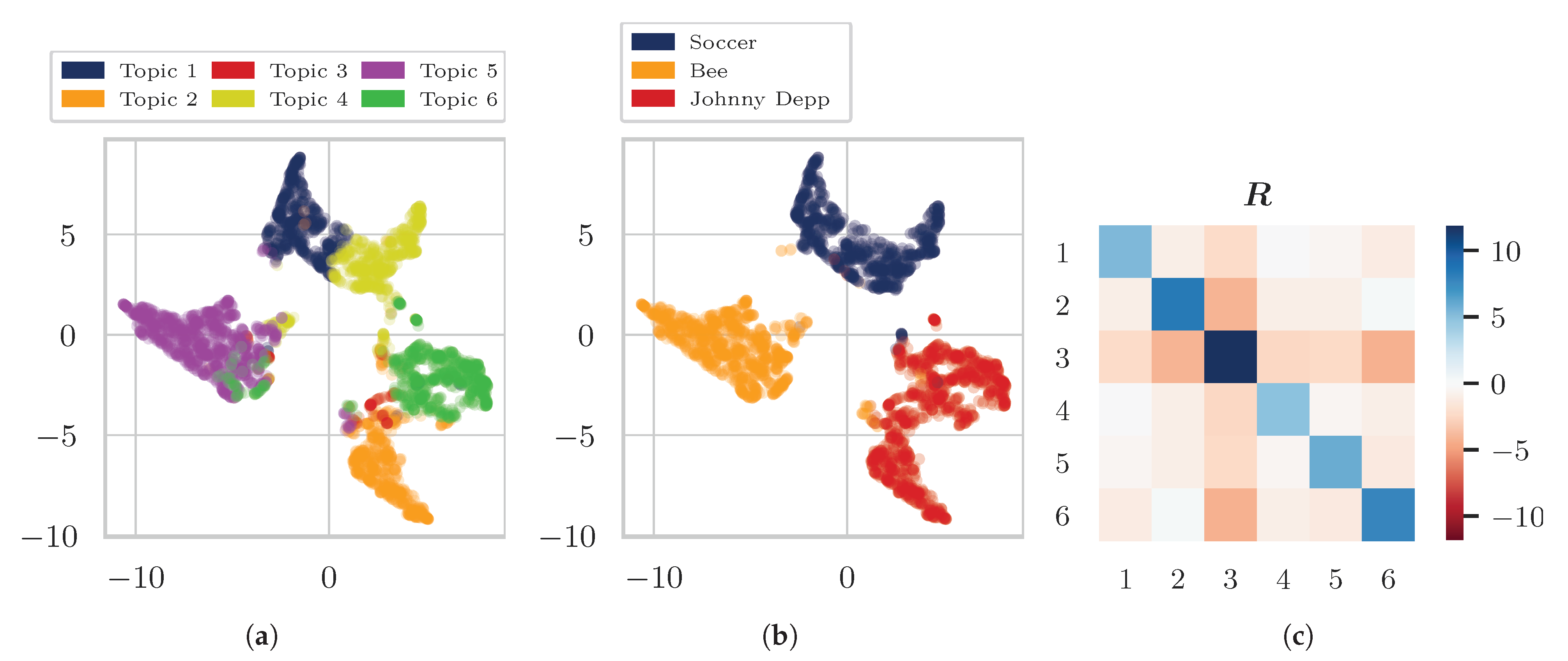
Further, we analyzed the relations between the topics by visualizing the trained R matrix as a heatmap (see Figure 5c).
Figure 5.
(a)2-dimensional representation of word embeddings colored by topic assignment). (b) 2-dimensional representation of word embeddings colored by original Wikipedia article assignment (words that occur in more than one article are excluded). (c) Colored heatmap of affinity matrix .
One thing to note was the symmetry of R which was a first indicator of a successful reconstruction, , (see Section 3.3). In addition, the main diagonal elements were consistently blue (positive), which suggested a high distinction between the topics. Although not very strong one could still see a connection between Topic 2 and 6 indicated by the light blue entry . While the suggested relation between Topic 1 and 4 was not clearly visible, element was the least negative one for Topic 1. In order to visualize the topic cluster quality we utilized Uniform Manifold Approximation ad Projection (UMAP) [24] to map the k-dimensional word embeddings to a 2-dimensional space. Figure 5a illustrates this low-dimensional representation of , where each word is colored based on the above described word to topic assignment. In conjunction with Table 5 one could nicely see that Topic 2 and 6 (Johnny Depp) and Topic 1 and 4 (Soccer) were close to each other. Hence, Figure 5a implicitly shows the learned topic relations as well.
As an additional benchmark, Figure 5b plots the same 2-dimensional representation, but now each word is colored based on the original Wikipedia article it belonged to. Words that occurred in more than one article were not considered in this plot.
Directly comparing Figure 5a,b shows that row-stochastic DEDICOM did not only recover the original articles but also found entirely new topics, which in this case represented subtopics of the articles. Let us emphasize that for all thematically similar article combinations, the found topics were usually not subtopics of a single article, but rather novel topics that might span across multiple Wikipedia articles (see for example Table A2 in the Appendix A). As mentioned at the top of this section, we are not only interested in learning meaningful topic clusters, but also in training interpretable word embeddings that capture semantic meaning.
Hence, we selected within each topic the two most representative words and calculated the cosine similarity between their word embeddings and all other word embeddings stored in . Table 6 shows the four nearest neighbors based on cosine similarity for the top two words in each topic. We observed a high thematical similarity between words with large cosine similarity, indicating the usefulness of the rows of as word embeddings.
Table 6.
For the most significant two words per topic, the four nearest neighbors based on cosine similarity are listed. Matrix trained on the wikipedia data as input matrix using automatic gradient methods.
In comparison to DEDICOM, other matrix factorization methods also provided a useful clustering of words into topics, with varying degree of granularity and clarity. However, the application of these methods as word embedding algorithms mostly failed on the word similarity task, with words close in cosine similarity seldom sharing the same thematical similarity we have seen in DEDICOM. This can be seen in Table A1, which shows for each method, NMF, LDA and SVD, the resulting word to topic clustering and the cosine nearest neighbors of the top two word embeddings per topic. While the individual topics extracted by NMF looked very reasonable, its word embeddings did not seem to carry any semantic meaning based on cosine similarity; e.g., the four nearest neighbors of “ball” were “invoke”, “replaced”, “scores” and “subdivided”. A similar nonsensical picture can be observed for the other main topic words. LDA and SVD performed slightly better on the similar word task, although not all similar words appeared to be sensible, e.g., “children”, “detective”, “crime”, “magazine” and “barber”. In addition, some topics could not be clearly defined due to mixed word assignments, e.g., Topic 4 for LDA and Topic 1 for SVD.
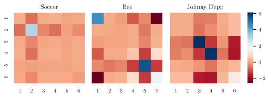
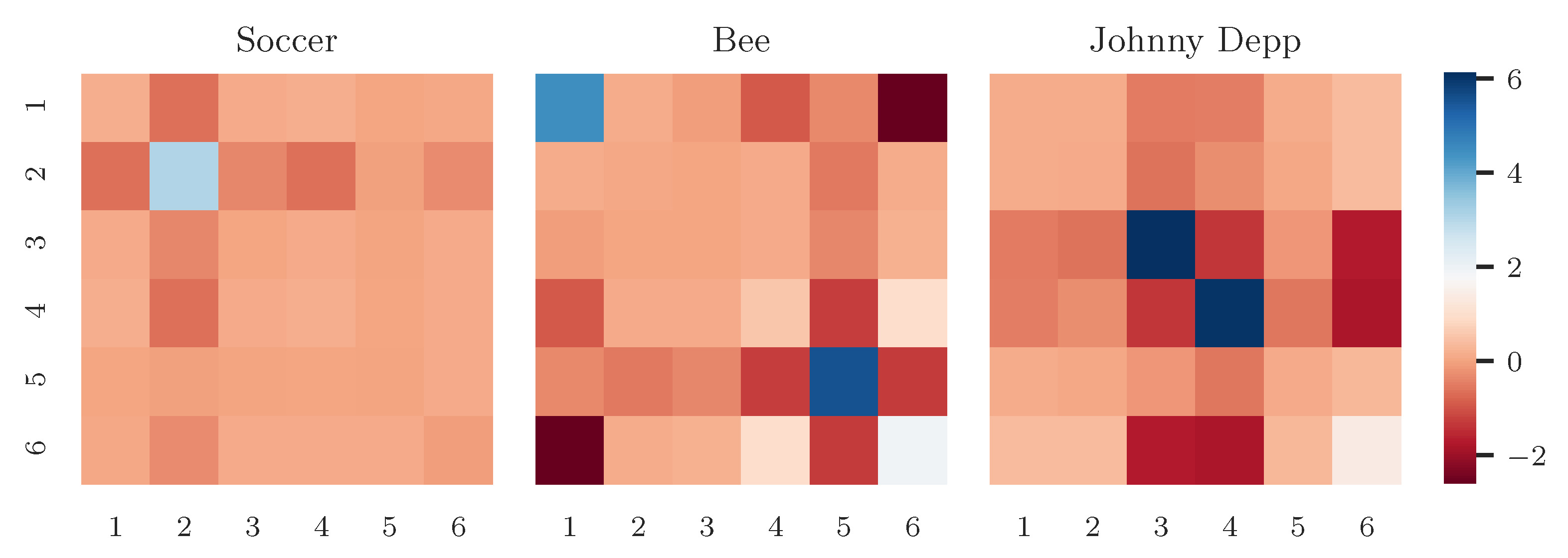
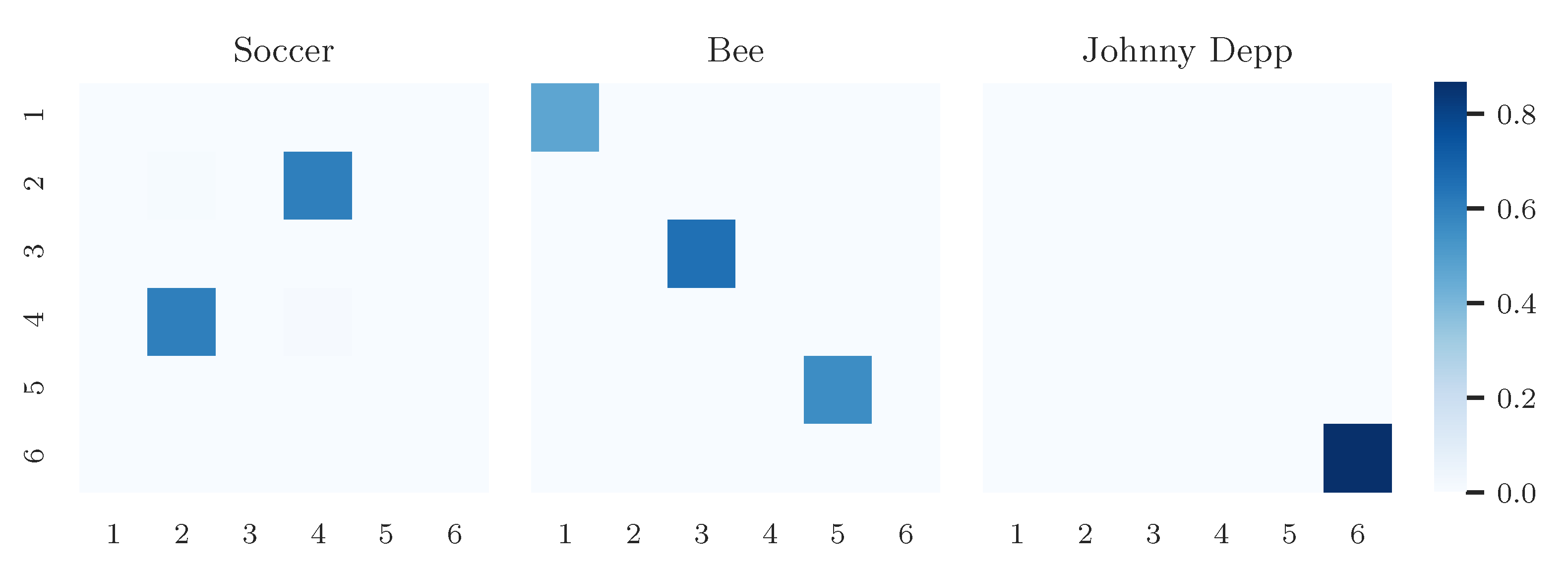
Before shifting our analysis to the Amazon movie review and the New York Times news corpus we investigated factorizing the tensor representation of the “Soccer, Bee and Johnny Depp” Wikipedia documents. In particular, we compared the qualitative factorization results of row-stochastic and non-negative tensor DEDICOM trained with automatic differentiation and multiplicative update rules, respectively. Table 7 and Table 8 in conjunction with Figure 6 and Figure 7 show the extracted topics and their relations for both methods.
Table 7.
Top 10 representative words per dimension of the basis matrix , trained on the wikipedia data as input tensor using automatic gradient methods.
Table 8.
Top 10 representative words per dimension of the basis matrix A, trained on the wikipedia data as input tensor using multiplicative update rules.
Figure 6.
Colored heatmap of affinity tensor , trained on the Wikipedia data represented as input tensor using automatic gradient methods.
Figure 7.
Colored heatmap of affinity tensor , trained on the Wikipedia data represented as input tensor using multiplicative update rules.
It could be seen that non-negative tensor DEDICOM yielded a more interpretable affinity tensor
(Figure 7) due to its enforced non-negativity. For example, it clearly highlighted the bee related Topics 1, 3 and 5 in the affinity tensor slice corresponding to the article “Bee”. Moreover, all extracted topics in Table 8 were distinct and their relations were well represented in the individual slices of . In contrast, Topic 6 in Table 7 did not represent a meaningful topic, which was also indicated by the low probability scores of the ranked topic words. Although the results of the similar word evaluation were arguably better for row-stochastic tensor DEDICOM (see Table 9 and Table 10) we prioritized topic extraction and relation quality. That is why in the further analysis of the Amazon review and New York Times news corpus we restricedt our evaluation to non-negative tensor DEDICOM.
Table 9.
For the most significant two words per topic, the four nearest neighbors based on cosine similarity are listed. Matrix , trained on the wikipedia data as input tensor using automatic gradient methods.
Table 10.
For the most significant two words per topic, the four nearest neighbors based on cosine similarity are listed. Matrix A, trained on the wikipedia data as input tensor using multiplicative update rules.
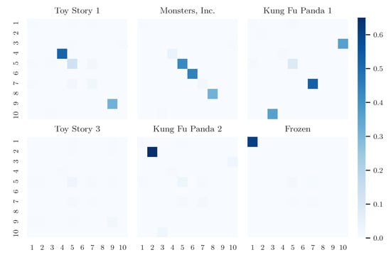
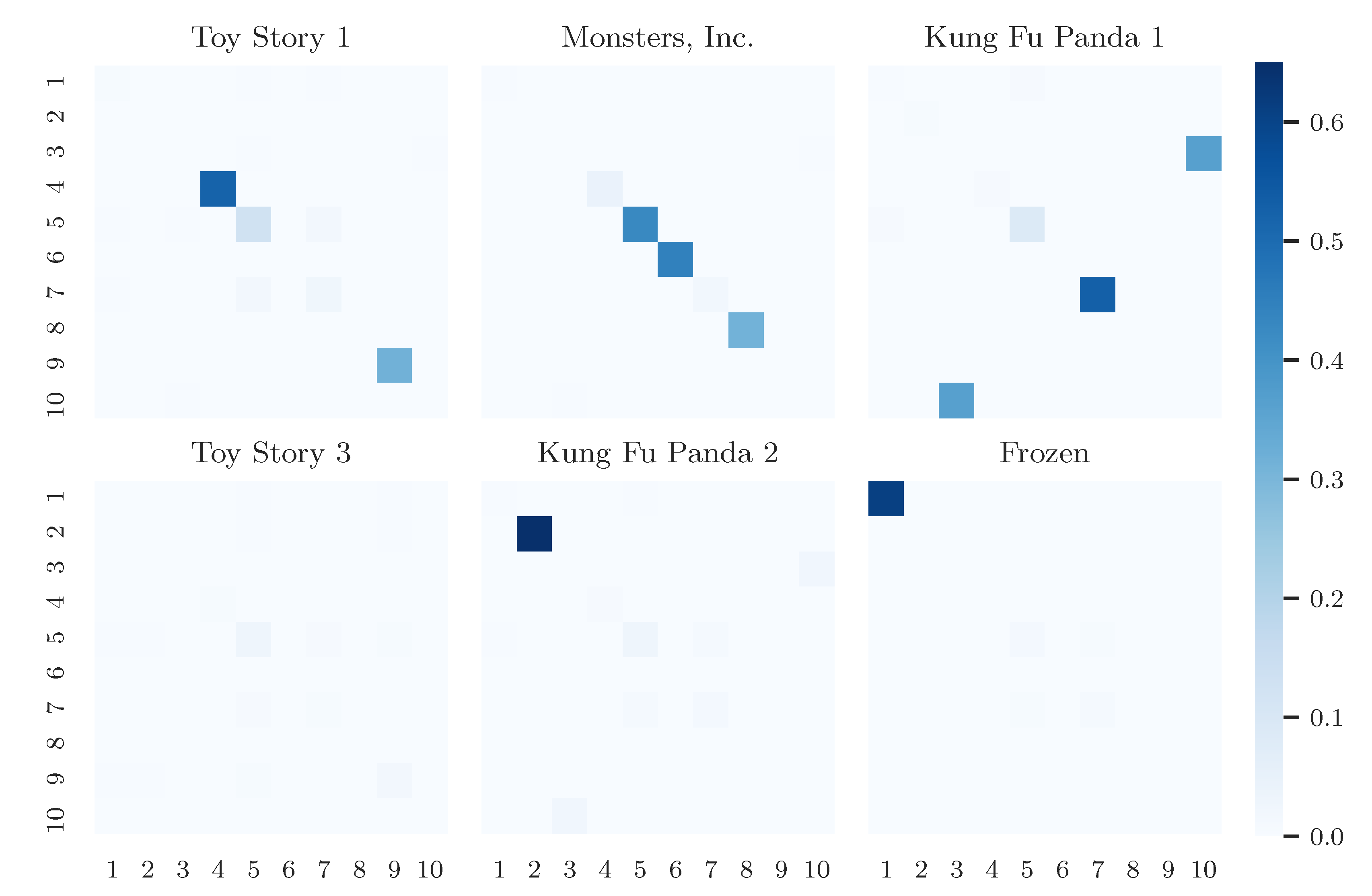
As described in Section 4.1 our Amazon movie review corpus comprised human written reviews for six famous animation films. Factorizing its PPMI tensor representation with non-negative tensor DEDICOM and the number of topics set to revealed not only movie-specific subtopics but also general topics that spanned over several movies. For example, Topics 1, 9 and 10 in Table 11 could uniquely be related to the films “Frozen”, “Toy Story 1” and “Kung Fu Panda 1”, respectively, whereas Topic 5 constituted bonus material on a DVD which held true for all films. The latter could also be seen in Figure 8 where Topic 5 was highlighted in each movie slice (strongly in the top and lightly in the bottom row). In the same sense one could observe that Topic 3 was present in both “Kung Fu Panda 1” and “Kung Fu Panda 2”, which is reasonable considering the topic depicted the general notion of a fearsome warrior.
Table 11.
Top 10 representative words per dimension of the basis matrix A, trained on the Amazon review data as input tensor using multiplicative update rules.
Figure 8.
Colored heatmap of affinity tensor , trained on the Amazon review data represented as input tensor using multiplicative update rules.
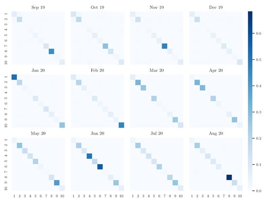
Figure 9 and Table 12 refer to our experimental results on the dataset of New York Times news articles. We saw a diverse array of topics extracted from the text corpus, ranging from US-politics (Topics 4, 6, 7) to natural disasters (Topic 8), Hollywood sexual assault allegations (Topic 10) and the COVID epidemic both from a medical view (Topic 3) and a view on resulting restrictions to businesses (Topic 9).
Figure 9.
Colored heatmap of affinity tensor , trained on the New York Times news article data represented as input tensor using multiplicative update rules.
Table 12.
Top 10 representative words per dimension of the basis matrix A, trained on the New York Times news article data as input tensor using multiplicative update rules.
The corresponding heatmap allowed us to infer when certain topics were most relevant in the last year. While the entries relating to the COVID pandemic remain light blue for the first half of the heatmap we sawa the articles picking up on the topic around March 2020, when the effects of the Coronavirus started hitting the US. Even comparatively smaller events like the conviction of Harvey Weinstein and the death of George Floyd triggering the racism debate in the US could be recognized in the heatmap, with a large deviation of Topic 10 around February 2020 and Topic 4 around June 2020.
Further empirical results on the Amazon review and New York Times news corpora, such as two-dimensional UMAP representations of the embedding matrix A and extracted topics from tensor NMF, can be found in Appendix A.3 and Appendix A.4, respectively. For example, Table A21 shows that the tensor NMF factorization also extracted high quality topics but lacked the interpretable affinity tensor R which was crucial in order to properly comprehend a topic development over time.
5. Conclusions and Outlook
We propose a constrained version of the DEDICOM algorithm that is able to factorize the pointwise mutual information matrices of text documents into meaningful topic clusters all the while providing interpretable word embeddings for each vocabulary item. Our study on semi-artificial data from Wikipedia articles has shown that this method recovers the underlying structure of the text corpus and provides topics with thematic granularity, meaning the extracted latent topics are more specific than a simple clustering of articles. A comparison to related matrix factorization methods has shown that the combination of relation aware topic modeling and interpretable word embedding learning given by our algorithm is unique in its class.
Extending this algorithm to factorize three-dimensional input tensors allows for the study of changes in the relations between topics across subsets of a structured text corpus, e.g., news articles grouped by time period. Algorithmically, this can be solved via alternating gradient descent by either automatic gradient methods or by applying multiplicative update rules which decrease training time drastically and enhance training stability.
Due to memory constraints from matrix multiplications of high dimensional dense tensors our proposed approach is currently limited in vocabulary size or time dimension.
In further work we aim for developing algorithms capable of leveraging sparse matrix multiplications to avoid the above mentioned memory constraints. In addition, we plan to expand on the possibilities of constraining the factor matrices and tensors when applying a multiplicative update rule and further analyze the behavior of the factor tensors, for example by utilizing time series analysis to discover temporal relations between extracted topics and to potentially identify trends. Finally, further analysis may include additional quantitative evaluations of our proposed methods’ topic modeling performance with competing approaches.
Author Contributions
Conceptualization, D.B.; Methodology, L.H.; Project administration, L.H. and D.B.; Supervision, C.B. and R.S.; Writing—original draft, L.H. and D.B. All authors have read and agreed to the published version of the manuscript.
Funding
The authors of this work were supported by the Competence Center for Machine Learning Rhine Ruhr (ML2R) which is funded by the Federal Ministry of Education and Research of Germany (grant no. 01|S18038C). We gratefully acknowledge this support.
Data Availability Statement
Publicly available datasets (Amazon reviews, Wikipedia articles) were analyzed in this study. This data can be found here: https://github.com/LarsHill/text-dedicom-paper. The NYT news article data presented in this study are available on request from the corresponding author. The data are not publicly available due to potential copyright concerns.
Conflicts of Interest
The authors declare no conflict of interest.
Appendix A. Additional Results
Appendix A.1. Additional Results on Wikipedia Data as Matrix Input
Articles: “Soccer”, “Bee”, “Johnny Depp”.
Table A1.
For each evaluated matrix factorization method we display the top 10 words for each topic and the five most similar words based on cosine similarity for the two top words from each topic.
Articles: “Dolphin”, “Shark”, “Whale”.
Table A2.
Top half lists the top 10 representative words per dimension of the basis matrix A, bottom half lists the five most similar words based on cosine similarity for the two top words from each topic.
Articles: “Dolphin”, “Shark”, “Whale’.
Table A3.
For each evaluated matrix factorization method we display the top 10 words for each topic and the five most similar words based on cosine similarity for the two top words from each topic.
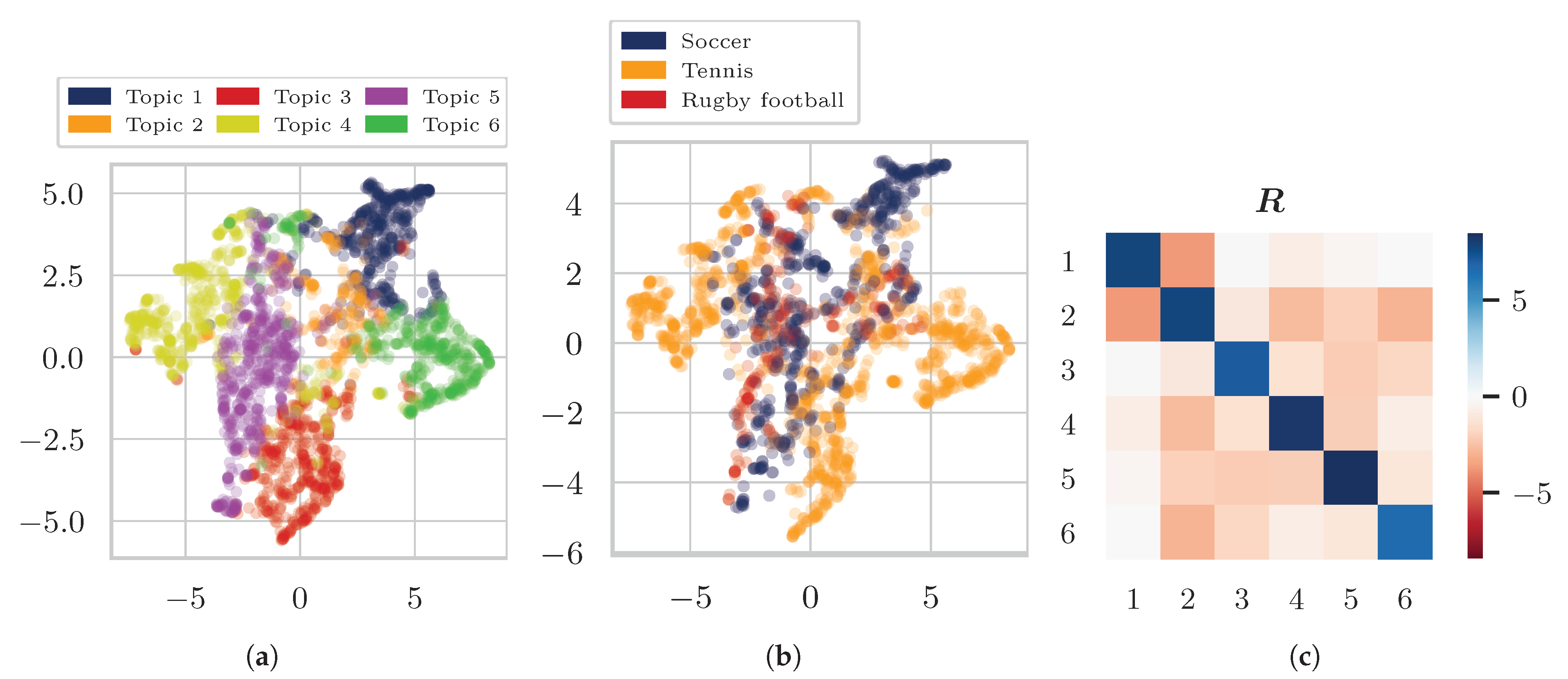
Articles: “Soccer”, “Tennis”, “Rugby”.
Table A4.
Top half lists the top 10 representative words per dimension of the basis matrix A, bottom half lists the five most similar words based on cosine similarity for the two top words from each topic.
Figure A1.
(a) 2-dimensional representation of word embeddings colored by topic assignment. (b) 2-dimensional representation of word embeddings colored by original Wikipedia article assignment (words that occur in more than one article are excluded). (c) Colored heatmap of affinity matrix .
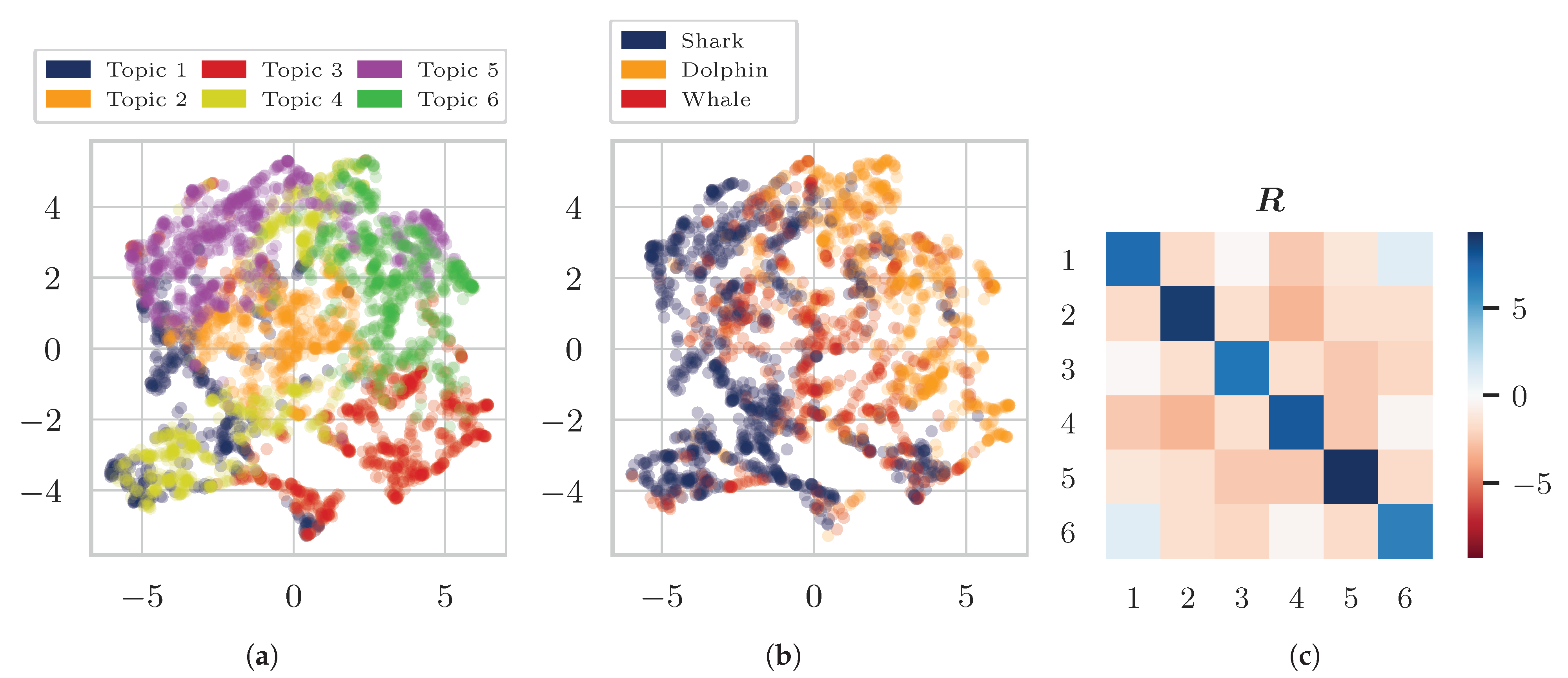
Figure A2.
(a) 2-dimensional representation of word embeddings colored by topic assignment. (b) 2-dimensional representation of word embeddings colored by original Wikipedia article assignment (words that occur in more than one article are excluded). (c) Colored heatmap of affinity matrix .
Articles: “Soccer”, “Tennis”, “Rugby”.
Table A5.
For each evaluated matrix factorization method we display the top 10 words for each topic and the 5 most similar words based on cosine similarity for the 2 top words from each topic.
Appendix A.2. Additional Results on Wikipedia Data as Tensor Input
Wikipedia Articles “Soccer”, “Bee”, “Johnny Depp”–DEDICOM Automatic gradient method.
Figure A3.
(a) 2-dimensional representation of word embeddings colored by topic assignment. (b) 2-dimensional representation of word embeddings colored by original Wikipedia article assignment (words that occur in more than one article are excluded).
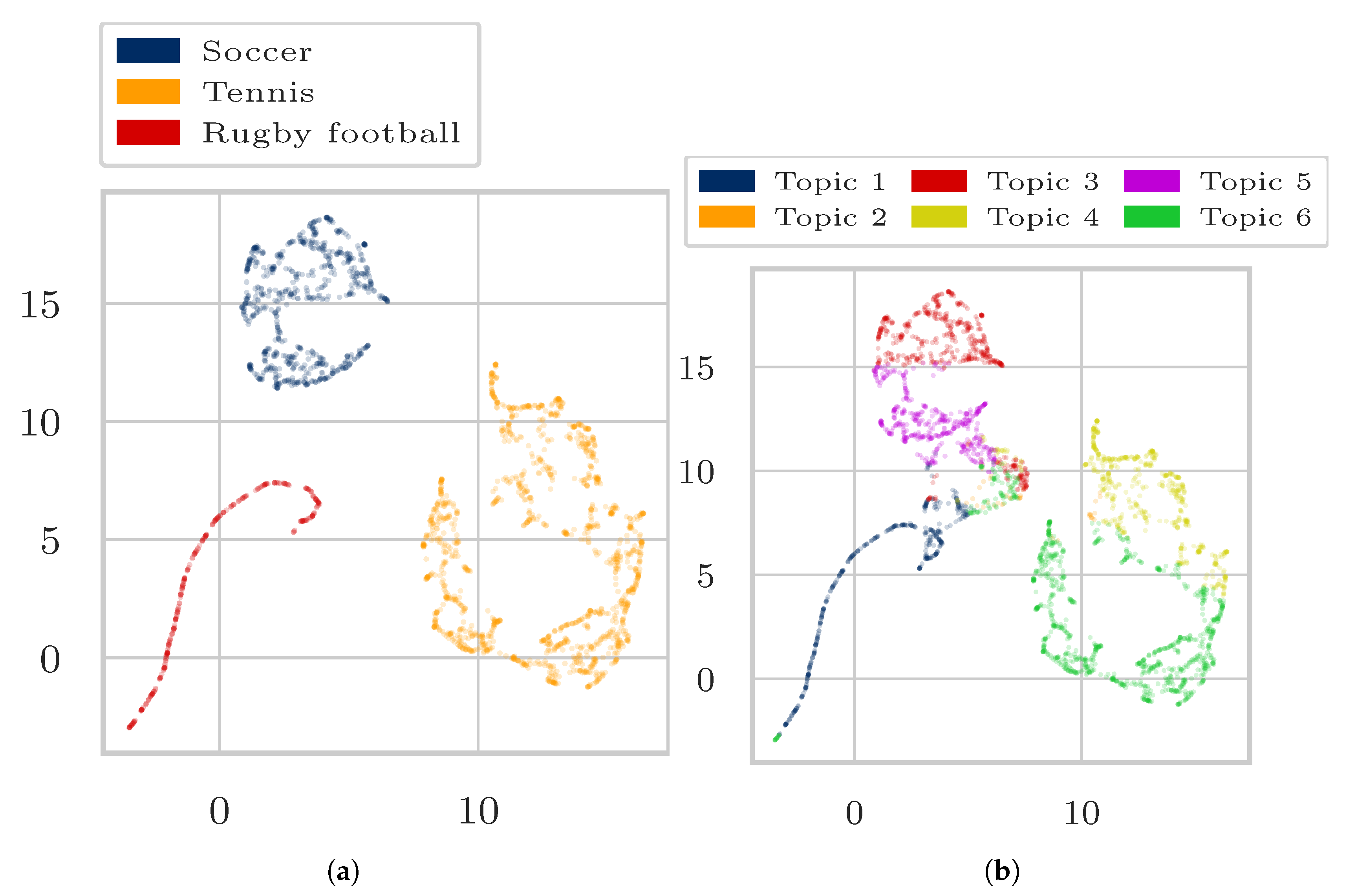
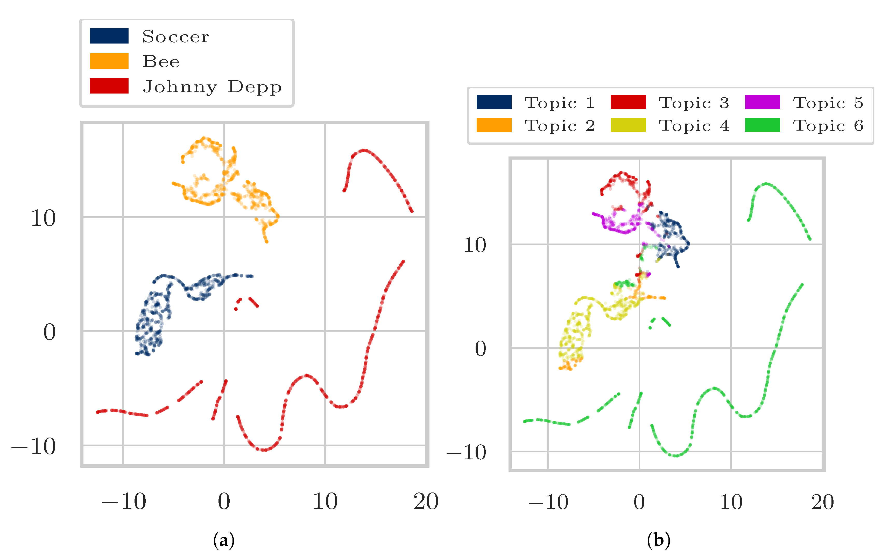
Wikipedia Articles “Soccer”, “Bee”, “Johnny Depp”—DEDICOM Multiplicative Update Rules.
Figure A4.
(a) 2-dimensional representation of word embeddings colored by topic assignment. (b) 2-dimensional representation of word embeddings colored by original Wikipedia article assignment (words that occur in more than one article are excluded).
Wikipedia Articles “Dolphin”, “Shark”, “Whale”—DEDICOM Multiplicative Update Rules.
Table A6.
Each column lists the top 10 representative words per dimension of the basis matrix A.
Table A7.
For the most significant two words per topic, the four nearest neighbors based on cosine similarity are listed.
Figure A5.
Colored heatmap of affinity tensor
.
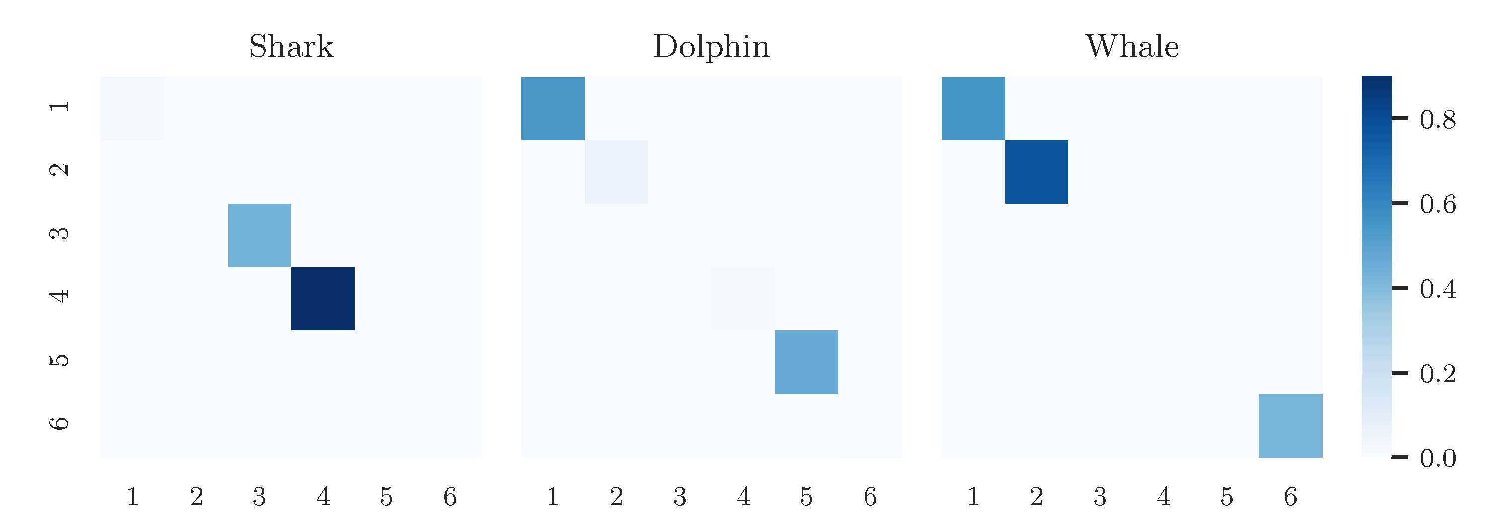
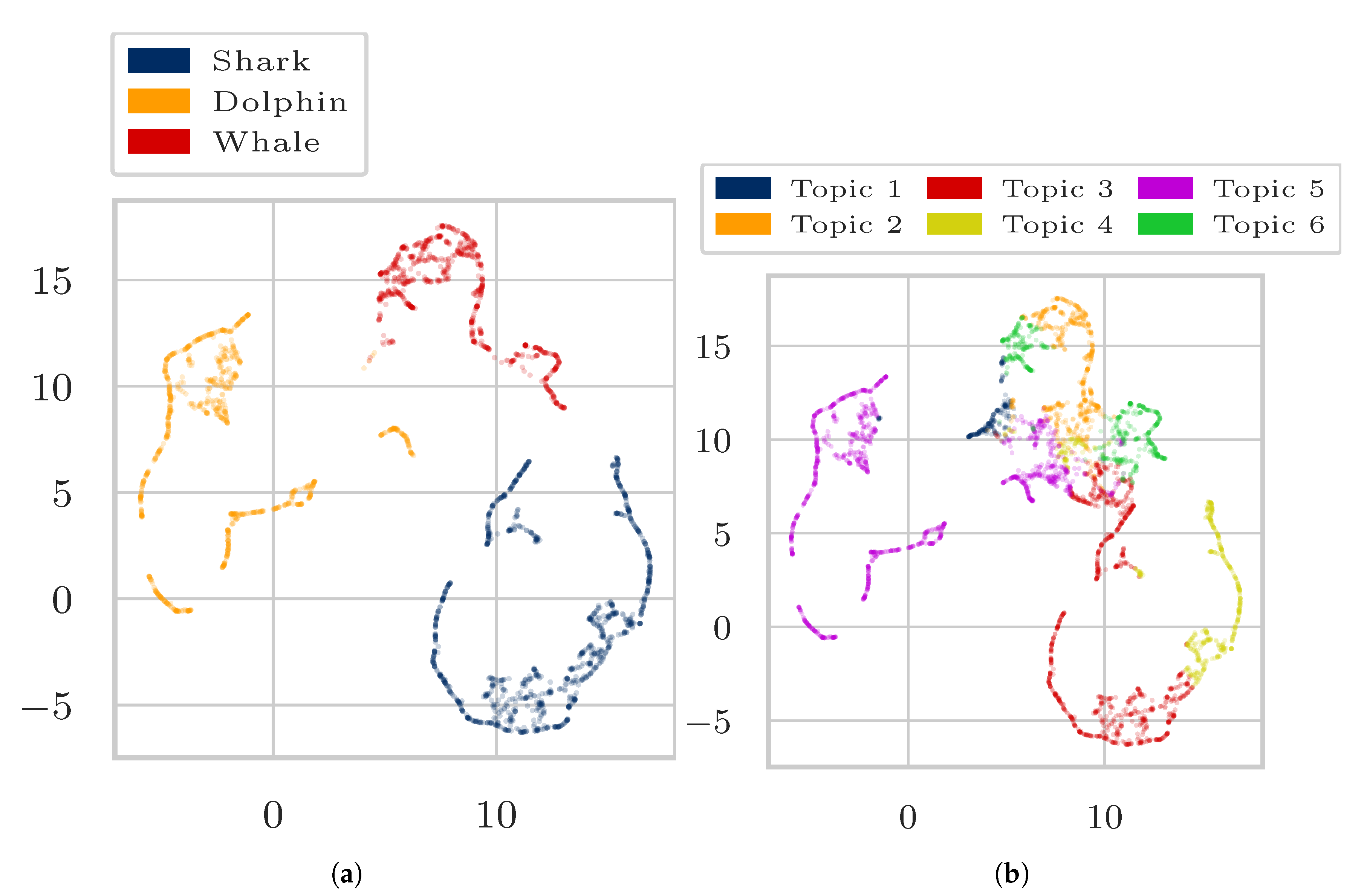
Figure A6.
(a) 2-dimensional representation of word embeddings A colored by topic assignment. (b) 2-dimensional representation of word embeddings A colored by original Wikipedia article assignment (words that occur in more than one article are excluded).
Wikipedia Articles “Soccer”, “Tennis”, “Rugby”—DEDICOM Multiplicative Update Rules.
Figure A7.
Colored heatmap of affinity tensor .
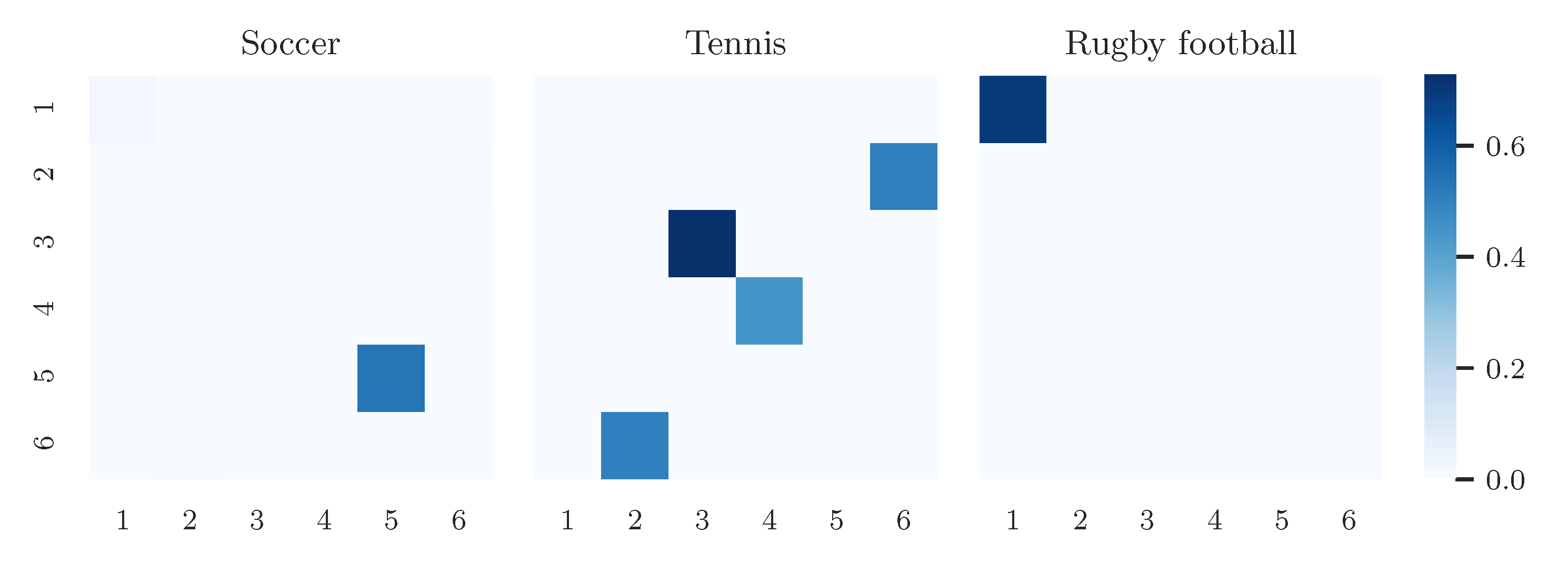
Table A8.
Each column lists the top 10 representative words per dimension of the basis matrix A.
Table A9.
For the most significant two words per topic, the four nearest neighbors based on cosine similarity are listed.
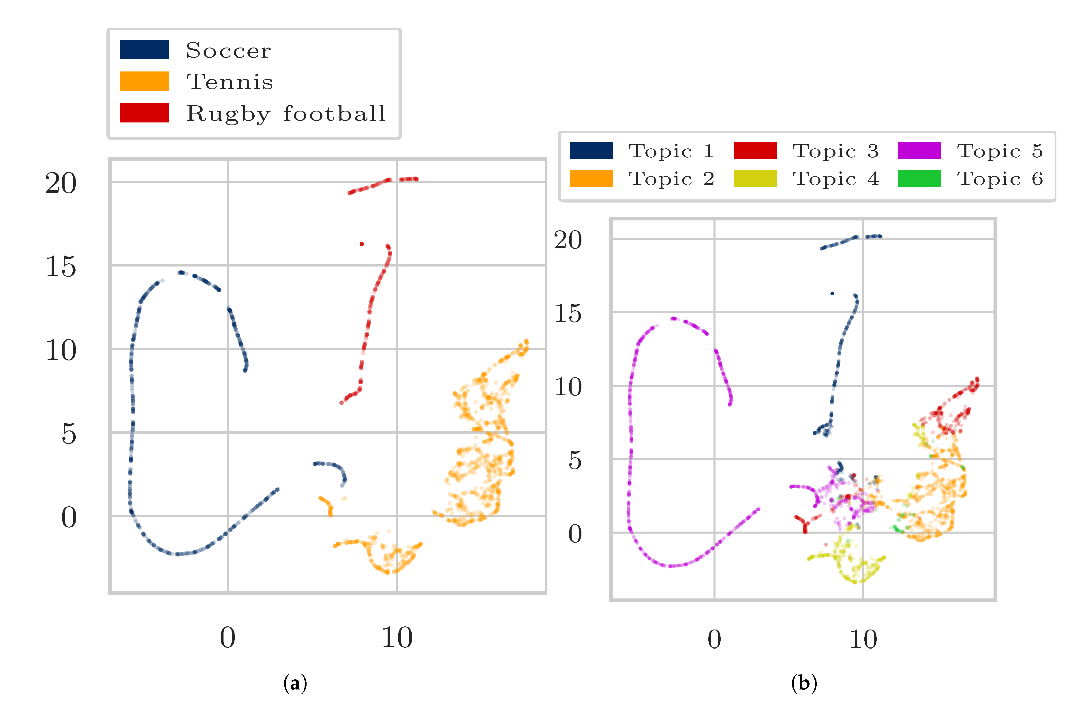
Figure A8.
(a) 2-dimensional representation of word embeddings colored by topic assignment. (b) 2-dimensional representation of word embeddings colored by original Wikipedia article assignment (words that occur in more than one article are excluded).
Wikipedia Articles “Soccer”, “Tennis”, “Rugby”—TNMF.
Table A10.
Each column lists the top 10 representative words per dimension of the basis matrix .
Table A11.
For the most significant two words per topic, the four nearest neighbors based on cosine similarity are listed.
Figure A9.
(a) 2-dimensional representation of word embeddings colored by topic assignment. (b) 2-dimensional representation of word embeddings colored by original Wikipedia article assignment (words that occur in more than one article are excluded).
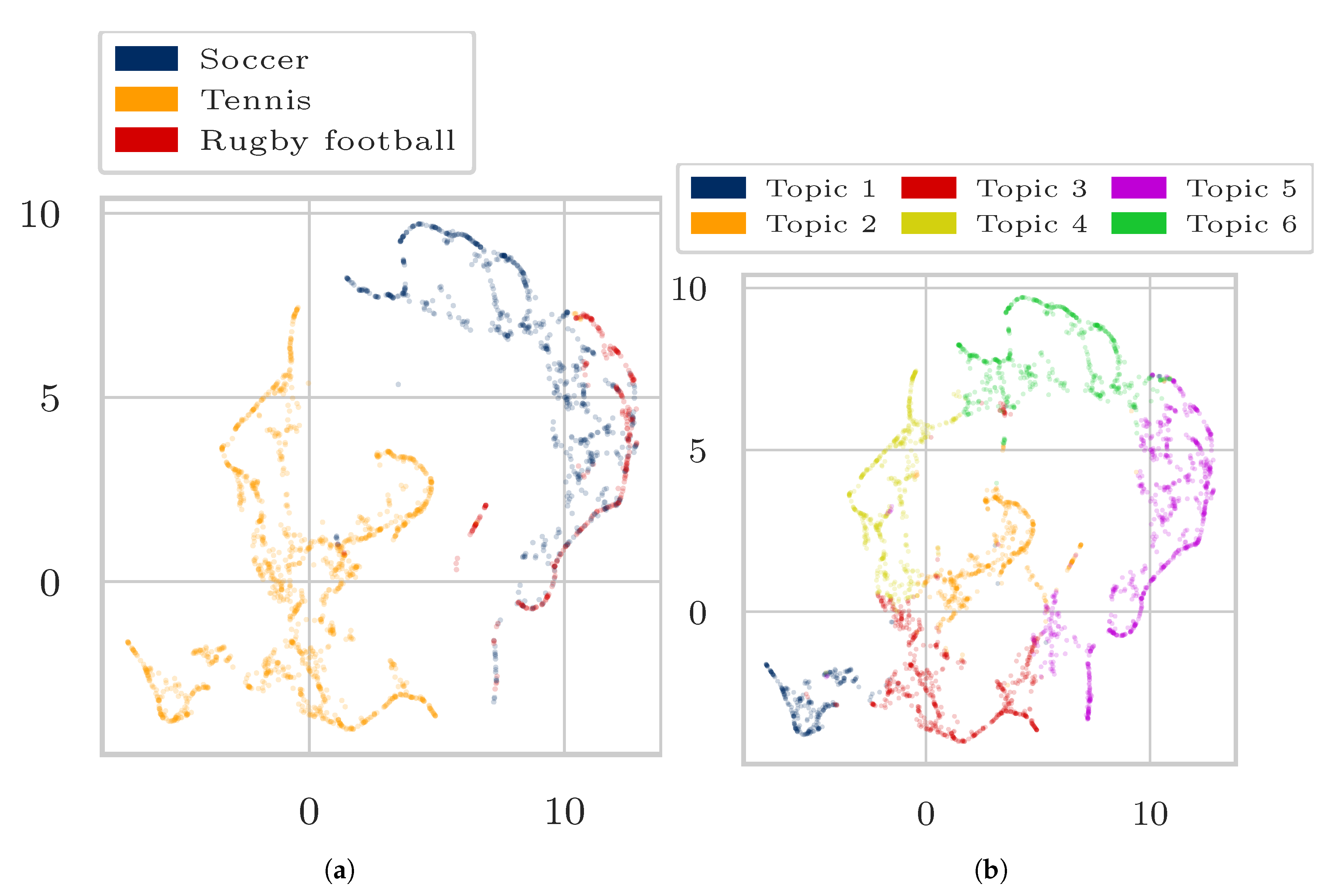
Wikipedia Articles “Dolphin”, “Shark”, “Whale”—TNMF.
Table A12.
Each column lists the top 10 representative words per dimension of the basis matrix H.
Table A13.
For the most significant two words per topic, the four nearest neighbors based on cosine similarity are listed.
Figure A10.
(a) 2-dimensional representation of word embeddings colored by topic assignment. (b) 2-dimensional representation of word embeddings colored by original Wikipedia article assignment (words that occur in more than one article are excluded).
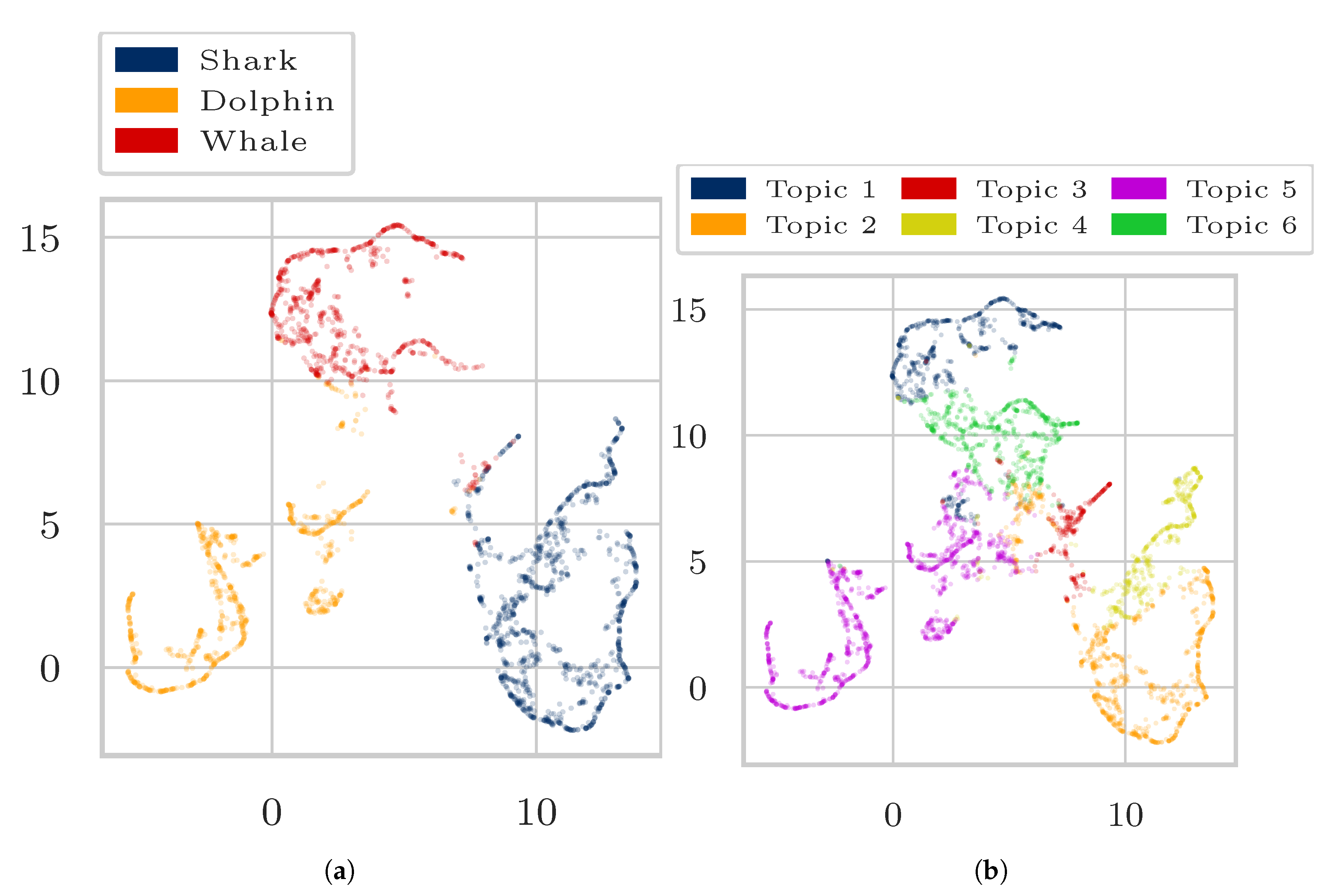
Wikipedia Articles “Soccer”, “Bee”, “Johnny Depp”—TNMF.
Table A14.
Each column lists the top 10 representative words per dimension of the basis matrix H.
Table A15.
For the most significant two words per topic, the four nearest neighbors based on cosine similarity are listed.
Appendix A.3. Additional Results on Amazon Review Data as Tensor Input
Amazon Reviews—DEDICOM Mulitplicative Update Rules.
Figure A11.
(a) 2-dimensional representation of word embeddings colored by topic assignment. (b) 2-dimensional representation of word embeddings colored by original Wikipedia article assignment (words that occur in more than one article are excluded).
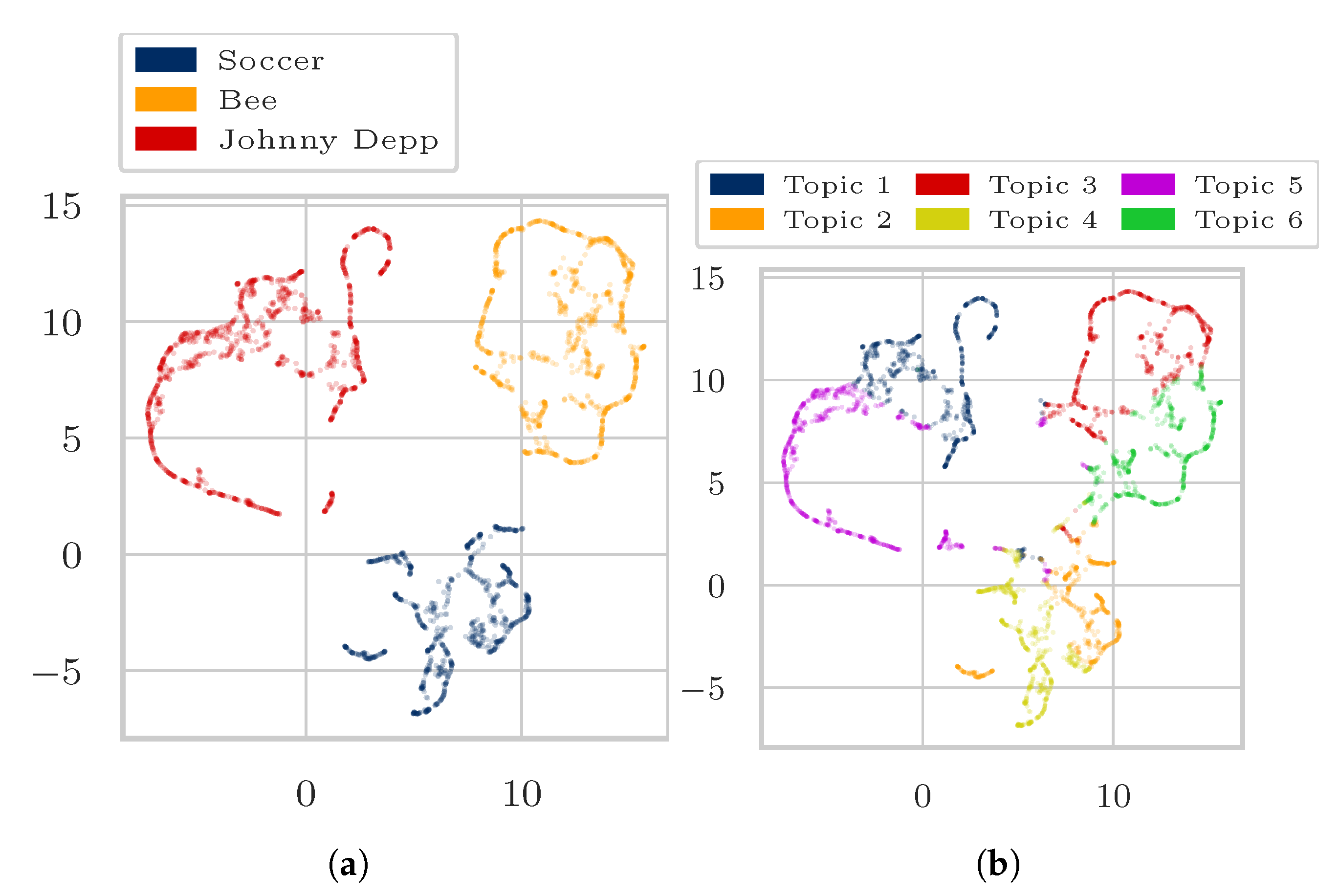
Figure A12.
(a) 2-dimensional representation of word embeddings A colored by topic assignment. (b) 2-dimensional representation of word embeddings A colored by original review article.
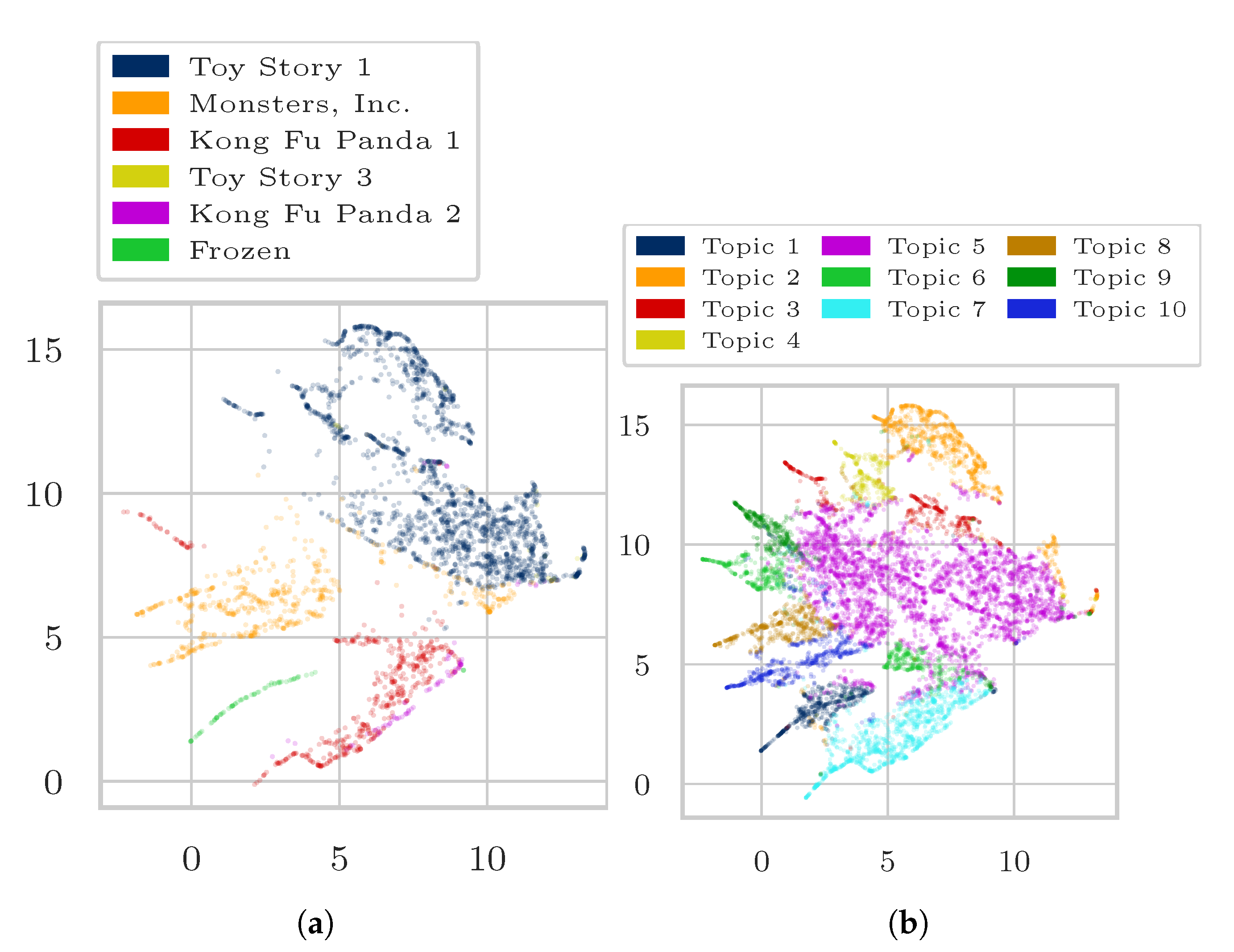
Figure A13.
(a) 2-dimensional representation of word embeddings colored by topic assignment. (b) 2-dimensional representation of word embeddings colored by original review article.
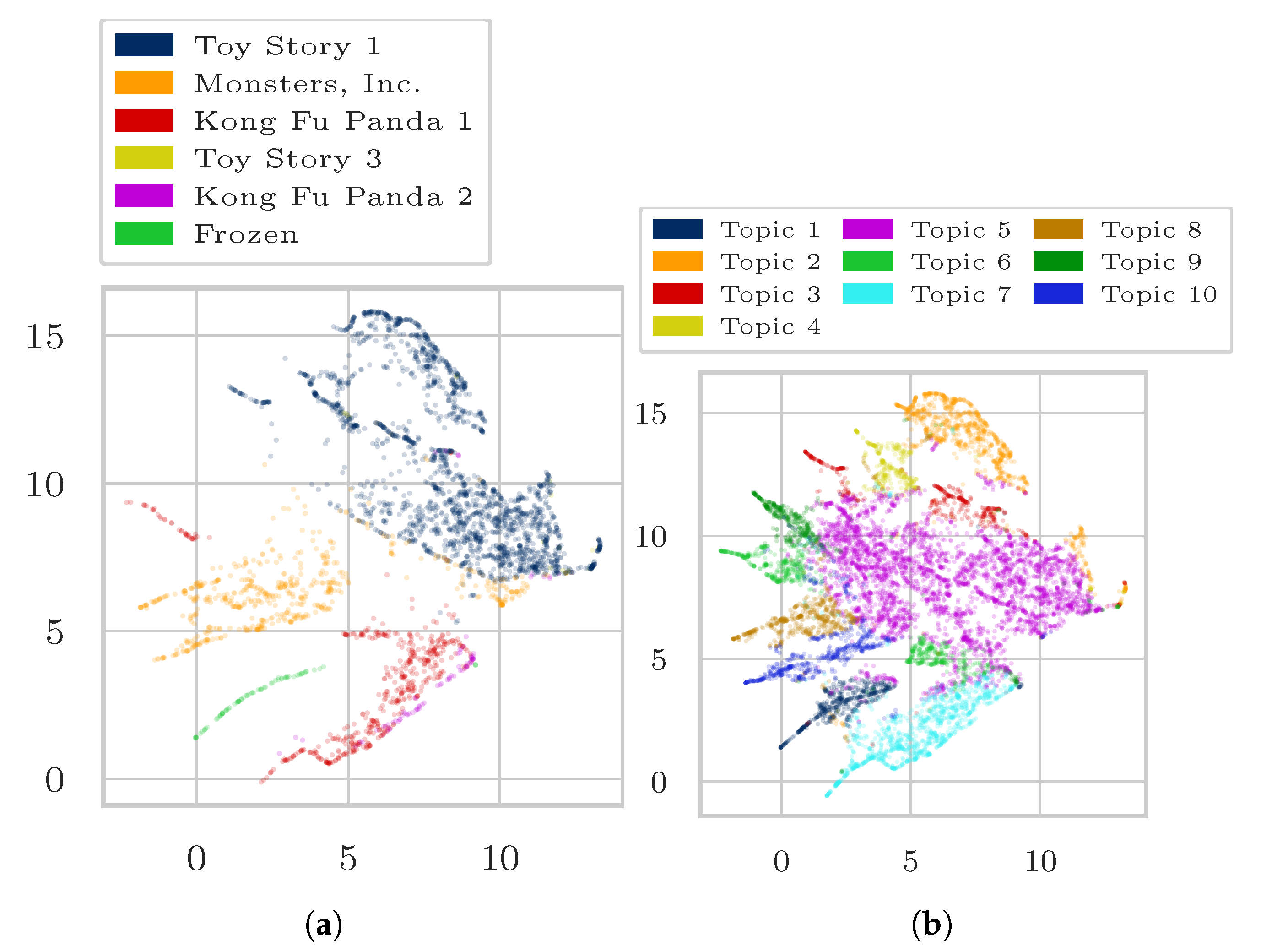
Table A16.
For the most significant two words per topic, the four nearest neighbors based on cosine similarity are listed.
Table A17.
For the most significant two words per topic, the four nearest neighbors based on cosine similarity are listed.
Amazon Reviews—TNMF.
Table A18.
Each column lists the top 10 representative words per dimension of the basis matrix H.
Table A19.
For the most significant two words per topic, the four nearest neighbors based on cosine similarity are listed.
Appendix A.4. Additional Results on the New York Times News Article Data as Tensor Input
New York Times News Articles—DEDICOM Mulitplicative Update Rules.
Table A20.
For the most significant two words per topic, the four nearest neighbors based on cosine similarity are listed.
New York Times News Articles—TNMF.
Table A21.
Each column lists the top 10 representative words per dimension of the basis matrix A.
Table A22.
For the most significant two words per topic, the four nearest neighbors based on cosine similarity are listed.
Figure A14.
2-dimensional representation of word embeddings A colored by topic assignment.
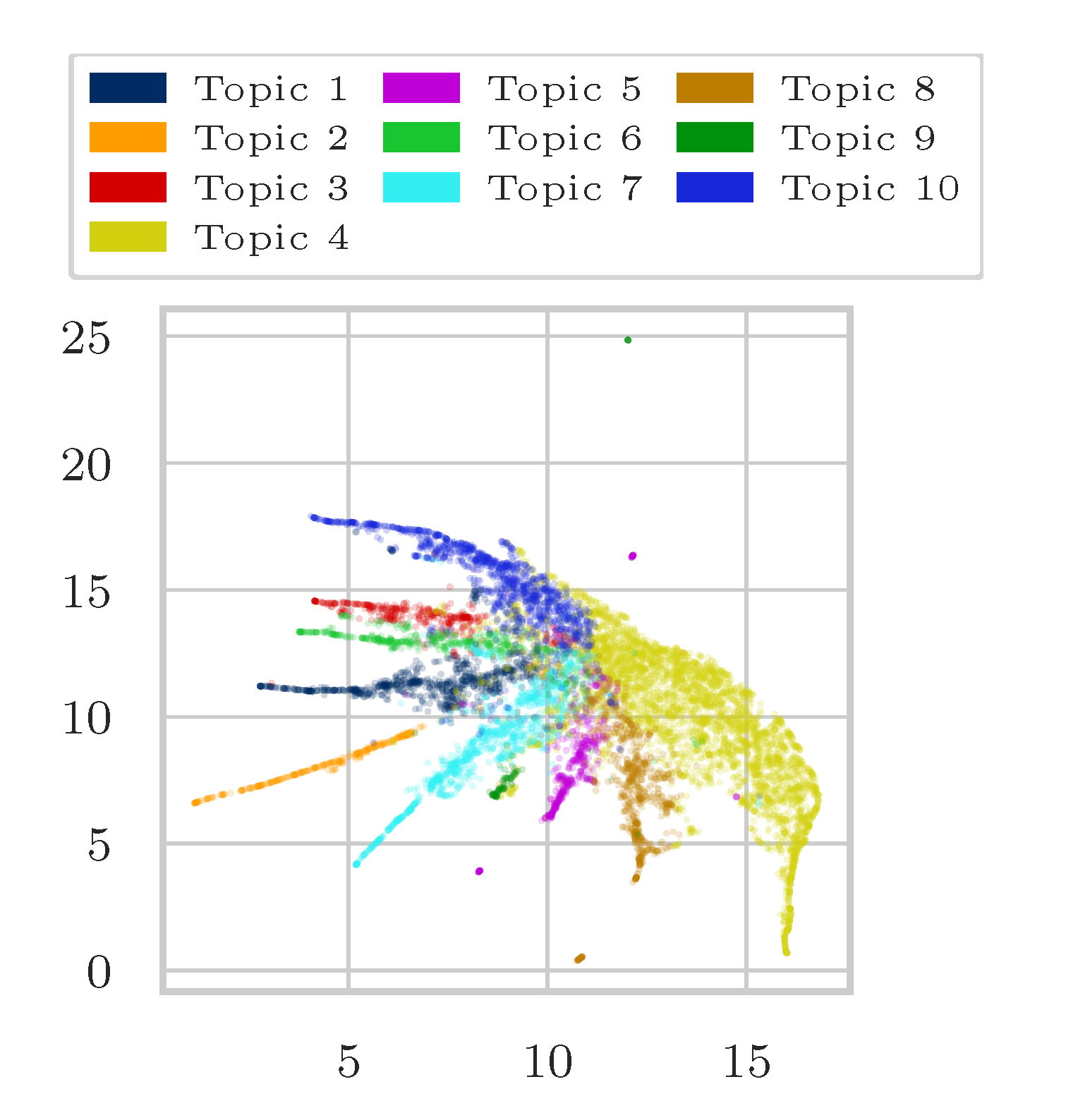
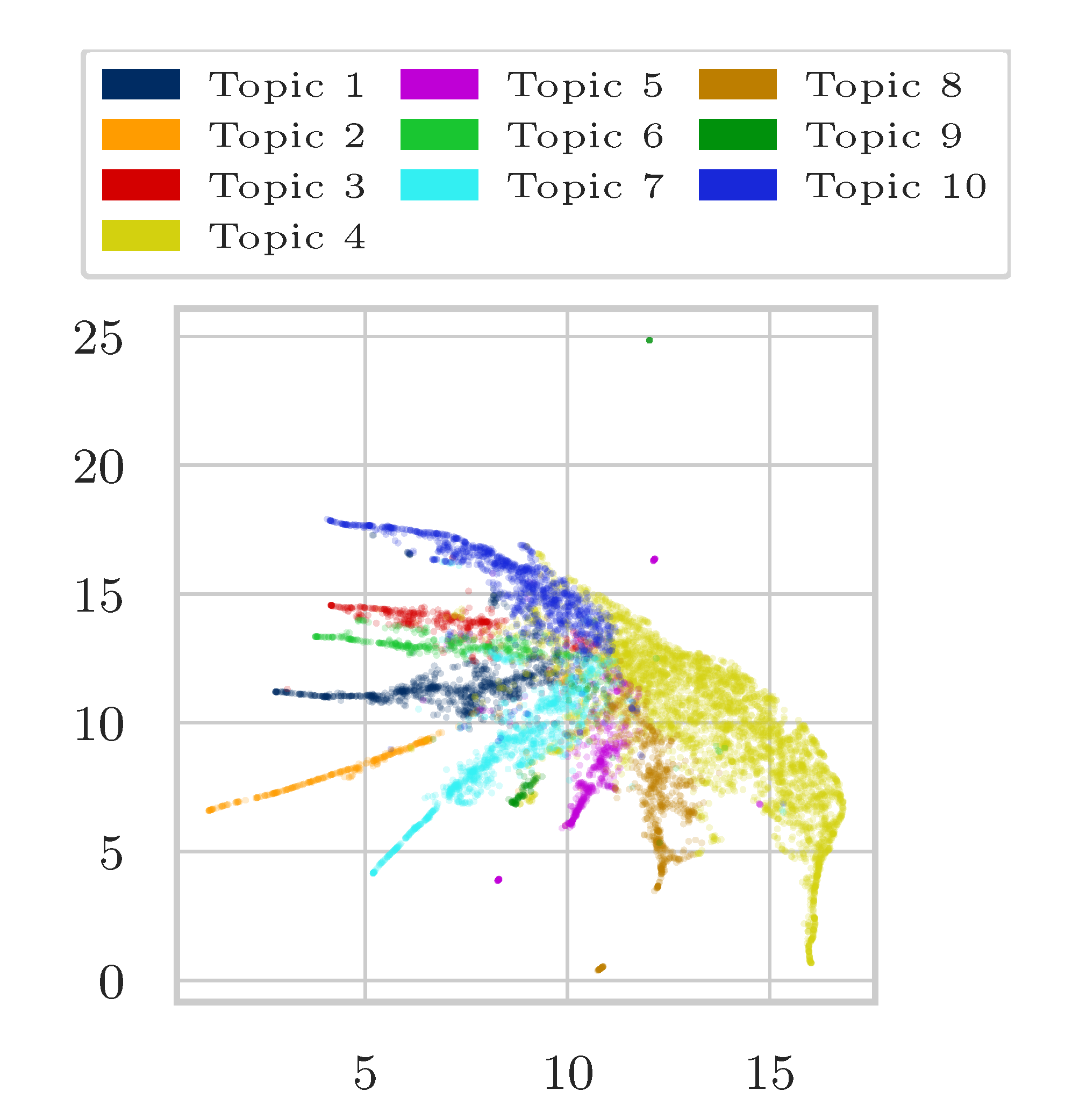
Figure A15.
2-dimensional representation of word embeddings colored by topic assignment).
References
- Levy, O.; Goldberg, Y. Neural Word Embedding as Implicit Matrix Factorization. In Advances in Neural Information Processing Systems; NIPS’14; MIT Press: Cambridge, MA, USA, 2014; Volume 2, pp. 2177–2185. [Google Scholar]
- Pennington, J.; Socher, R.; Manning, C. Glove: Global Vectors for Word Representation. In Proceedings of the 2014 Conference on Empirical Methods in Natural Language Processing (EMNLP), Association for Computational Linguistics, Doha, Qatar, 25–29 October 2014; pp. 1532–1543. [Google Scholar]
- Hillebrand, L.P.; Biesner, D.; Bauckhage, C.; Sifa, R. Interpretable Topic Extraction and Word Embedding Learning Using Row-Stochastic DEDICOM. In Machine Learning and Knowledge Extraction—4th International Cross-Domain Conference, CD-MAKE; Lecture Notes in Computer Science; Springer: Dublin, Ireland, 2020; Volume 12279, pp. 401–422. [Google Scholar]
- Symeonidis, P.; Zioupos, A. Matrix and Tensor Factorization Techniques for Recommender Systems; Springer International Publishing: New York, NY, USA, 2016. [Google Scholar] [CrossRef] [Scilit]
- Harshman, R.; Green, P.; Wind, Y.; Lundy, M. A Model for the Analysis of Asymmetric Data in Marketing Research. Market. Sci. 1982, 1, 205–242. [Google Scholar] [CrossRef] [Scilit]
- Andrzej, A.H.; Cichocki, A.; Dinh, T.V. Nonnegative DEDICOM Based on Tensor Decompositions for Social Networks Exploration. Aust. J. Intell. Inf. Process. Syst. 2010, 12, 10–15. [Google Scholar]
- Bader, B.W.; Harshman, R.A.; Kolda, T.G. Pattern Analysis of Directed Graphs Using DEDICOM: An Application to Enron Email; Office of Scientific & Technical Information Technical Reports; Sandia National Laboratories: Albuquerque, NM, USA, 2006. [Google Scholar]
- Sifa, R.; Ojeda, C.; Cvejoski, K.; Bauckhage, C. Interpretable Matrix Factorization with Stochasticity Constrained Nonnegative DEDICOM. In Proceedings of the KDML-LWDA, Rostock, Germany, 11–13 September 2017. [Google Scholar]
- Sifa, R.; Ojeda, C.; Bauckage, C. User Churn Migration Analysis with DEDICOM. In Proceedings of the 9th ACM Conference on Recommender Systems; RecSys ’15; Association for Computing Machinery: New York, NY, USA, 2015; pp. 321–324. [Google Scholar]
- Chew, P.; Bader, B.; Rozovskaya, A. Using DEDICOM for Completely Unsupervised Part-of-Speech Tagging. In Proceedings of the Workshop on Unsupervised and Minimally Supervised Learning of Lexical Semantics, Boulder, CO, USA, 5 June 2009; Association for Computational Linguistics: Boulder, CO, USA, 2009; pp. 54–62. [Google Scholar]
- Nickel, M.; Tresp, V.; Kriegel, H.P. A Three-Way Model for Collective Learning on Multi-Relational Data. In Proceedings of the 28th International Conference on Machine Learning, Bellevue, WA, USA, 28 June–2 July 2009; Association for Computing Machinery: Bellevue, WA, USA, 2011; pp. 809–816. [Google Scholar]
- Sifa, R.; Yawar, R.; Ramamurthy, R.; Bauckhage, C.; Kersting, K. Matrix- and Tensor Factorization for Game Content Recommendation. KI-Künstl. Intell. 2019, 34, 57–67. [Google Scholar] [CrossRef] [Scilit]
- Mikolov, T.; Sutskever, I.; Chen, K.; Corrado, G.; Dean, J. Distributed Representations of Words and Phrases and their Compositionality. Adv. Neural Inf. Proc. Syst. 2013, arXiv:cs.CL/1310.454626, 3111–3119. [Google Scholar]
- Lee, D.D.; Seung, H.S. Algorithms for Non-Negative Matrix Factorization. In Proceedings of the 13th International Conference on Neural Information Processing Systems; NIPS’00; MIT Press: Cambridge, MA, USA, 2000; pp. 535–541. [Google Scholar]
- Furnas, G.W.; Deerwester, S.; Dumais, S.T.; Landauer, T.K.; Harshman, R.A.; Streeter, L.A.; Lochbaum, K.E. Information Retrieval Using a Singular Value Decomposition Model of Latent Semantic Structure. In ACM SIGIR Forum; ACM: New York, NY, USA, 1988. [Google Scholar]
- Wang, Y.; Zhu, L. Research and implementation of SVD in machine learning. In Proceedings of the 2017 IEEE/ACIS 16th International Conference on Computer and Information Science (ICIS), Wuhan, China, 24–26 May 2017; pp. 471–475. [Google Scholar]
- Jolliffe, I. Principal Component Analysis; John Wiley and Sons Ltd.: Hoboken, NJ, USA, 2005. [Google Scholar]
- Blei, D.M.; Ng, A.Y.; Jordan, M.I. Latent Dirichlet Allocation. J. Mach. Learn. Res. 2003, 3, 993–1022. [Google Scholar]
- Lebret, R.; Collobert, R. Word Embeddings through Hellinger PCA. In Proceedings of the 14th Conference of the European Chapter of the Association for Computational Linguistics, Gothenburg, Sweden, 26–30 April 2014; pp. 482–490. [Google Scholar]
- Nguyen, D.Q.; Billingsley, R.; Du, L.; Johnson, M. Improving Topic Models with Latent Feature Word Representations. Trans. Assoc. Comput. Linguist. 2015, 3, 299–313. [Google Scholar] [CrossRef] [Scilit]
- Frank, M.; Wolfe, P. An algorithm for quadratic programming. Naval Res. Logist. Q. 1956, 3, 95–110. [Google Scholar] [CrossRef] [Scilit]
- Ni, J.; Li, J.; McAuley, J. Justifying recommendations using distantly-labeled reviews and fine-grained aspects. In Proceedings of the 2019 Conference on Empirical Methods in Natural Language Processing and the 9th International Joint Conference on Natural Language Processing (EMNLP-IJCNLP), Hong Kong, China, 3–7 November 2019; pp. 188–197. [Google Scholar]
- Kingma, D.P.; Ba, J. Adam: A method for stochastic optimization. arXiv 2014, arXiv:1412.6980. [Google Scholar]
- McInnes, L.; Healy, J.; Melville, J. UMAP: Uniform Manifold Approximation and Projection for Dimension Reduction. arXiv 2018, arXiv:1802.03426. [Google Scholar]




Publisher’s Note: MDPI stays neutral with regard to jurisdictional claims in published maps and institutional affiliations. |
© 2021 by the authors. Licensee MDPI, Basel, Switzerland. This article is an open access article distributed under the terms and conditions of the Creative Commons Attribution (CC BY) license (http://creativecommons.org/licenses/by/4.0/).