


Abstract
Low-pressure carburizing (LPC) models can support recipe screening, but numerical agreement must be separated from experimental validation and calibration. A one-dimensional model using concentration-dependent Ågren diffusivity, a prescribed boost carbon flux, zero-flux diffusion windows, a carbide reservoir and a non-isothermal tail is compared with four industrial trials on 16MnCr5 at 940–950 °C. Numerical verification includes an analytical solution, grid refinement and an independent COMSOL implementation. With no parameter fitted to this campaign, depths at 0.36 wt.% C are 894 and 866 µm for two free-surface trials, compared with hardness-based CHD550 values of 1036 and 907 µm measured at HV0.3: point deviations of −13.7% and −4.6%. A joint flux fit gives residuals of −4.9% and +5.2%; two-point leave-one-out transfer gives +10.6% and −9.6%. These are conditional deviations, not uncertainty-inclusive accuracy bounds. An empirical hardness bridge changes the uncalibrated depths by about 11%, and the available hardness traverses do not support statistical confidence intervals. The primary experimental limitation is the absence of measured carbon profiles: comparison is restricted to depth criteria, and predicted surface concentrations remain unverified. Flux and diffusivity sensitivities are nearly collinear for the two schedules. A single bore observation is 36% shallower than a free-surface observation from another trial, with unresolved load, quench and laboratory effects. Nominal gas-supply calculations suggest scope for flow-reduction experiments but disagree with cylinder weighing and do not establish transfer efficiency. The practical application is preliminary recipe screening and selection of informative follow-up measurements within the studied conditions; broader accuracy, concentration-profile validation and geometry corrections require further experiments.
1. Introduction
Low-pressure carburizing with acetylene is used for case-hardening engineering steels and can be combined with high-pressure gas quenching [1,2,3]. Carbon is introduced during short boost pulses at low pressure and redistributed during subsequent diffusion periods under vacuum; this boost–diffuse description is established in pulse-carburizing and surface-transfer studies [4,5,6]. The pulse durations and their spacing therefore influence the carbon profile as well as the total treatment time.
LPC recipe calculation couples surface transfer to carbon diffusion. Published approaches resolve reactive acetylene flow and pyrolysis [7], impose a calibrated surface flux [4], or include transient carbide formation during pulse carburizing [5]. Surface kinetics depend on the steel and operating conditions [1,6]. A prescribed constant flux is a useful reduced model, but gas availability, evolving surface concentration and reaction products can make the actual uptake time dependent.
Industrial usefulness also depends on how a model is assessed. A prediction made before a trial, an uncalibrated calculation with inherited parameters, and a fit to the same trial answer different questions. Published studies address carbon profiles, hardness, quenching and distortion with different levels of coupling and calibration [2,3,8]. The present study explicitly separates a recorded pre-campaign recipe-designer output from the uncalibrated flux-model comparison and from subsequent one-parameter fits.
Coupled reactive-flow simulations have connected gas composition, surface reaction and diffusion in the steel [9]. Experiments on 20MnCr5 at 940 °C show that carbon enrichment and carbide response evolve during individual boosts [10], while segmented-flux modelling explicitly treats changes in transfer [4]. Composition-dependent carbon and cementite profiles measured by GD-OES, diffraction and electron-probe analysis show why a single alloy multiplier and a saturation reservoir remain approximations [11]. These studies motivate testing uptake and diffusivity separately rather than interpreting every case-depth discrepancy as an error in one transport coefficient. Austenite grain growth has also been studied separately in high-temperature LPC [12]; it is not predicted by the present diffusion model.
Gas-flow optimization also depends on pressure, load area and geometry. An industrial 16MnCr5 study reduced mixture use by adapting supply to calculated demand [13], whereas controlled gravimetric experiments on the same grade found pressure-dependent flow effects on carbon uptake [14]. Nominal chamber supply is therefore insufficient to establish uniform local availability. Hardness introduces another evidence boundary: experiments using SEM and XRD have found different carbide and retained-austenite states despite similar case-hardness measures [15]. The present depth comparisons cannot independently validate concentration or phase distributions.
Four LPC trials were run on 16MnCr5 in a production vacuum furnace at 940–950 °C. The recipe used for Tests 3 and 4 and its predicted depth were recorded by the original design tool before the trials. Hardness traverses were later obtained at an accredited external laboratory or at the university laboratory. The corrected flux model was evaluated without fitting its baseline parameters to those traverses; this was distinguished from the independently documented pre-campaign design prediction.
Four questions are asked, each of which can be answered incorrectly by the data:
- How large is the case-depth error of a physics-based LPC model on this steel and this furnace when no parameters have been fitted to the campaign?
- How do inherited concentration-driven recipe predictions and controlled boost-boundary comparisons differ from the prescribed-flux calculation under the studied schedules?
- If a single parameter is calibrated, which parameter is it—and can case-depth data even distinguish the candidates?
- Which observations fall outside the scope of the one-dimensional free-surface model, and what measurements are needed to test those limitations?
The under-carburized trial, the bore traverse and the discrepancy between acetylene set-point estimates and cylinder weighing are retained. They constrain the interpretation of model accuracy, geometry and gas consumption rather than providing independent validation of all three.
2. Materials and Methods
2.1. Evidence Hierarchy
Three levels of evidence are kept separate throughout and are never merged into a single accuracy claim:
- a
- Numerical verification—evidence that the code solves the equations it states: an analytical bench-mark, a grid-convergence study and an independent commercial finite-element implementation of the same formulation. It involves no experiment and no adjustable parameter.
- b
- Uncalibrated comparison—the revised model uses inherited parameters without fitting them to the campaign. The separately recorded pre-campaign prediction belongs to the original recipe designer; no dated pre-trial output of the revised flux formulation is used to claim prospective validation.
- c
- Calibration and transfer—one scalar is fitted to campaign data, with joint-fit residuals separated from leave-one-out transfer between the two free-surface trials. Neither provides a population prediction interval.
The experimental comparison concerns hardness-based depths at HV0.3. The calculated carbon-threshold depth is a distinct observable linked to them by an assumed conversion. Carbon concentrations, retained austenite and residual stresses were not measured; surface and core hardness were measured but are not validated outputs of the diffusion model.
2.2. Material
All modelled specimens were 16MnCr5+H cylinders of Ø29 × 150 mm from one steelmaking heat (2323340V, Deutsche Edelstahlwerke Specialty Steel GmbH & Co. KG, Witten, Germany), produced by an electric arc furnace (EAF, Carbolite GmbH, Germany), ladle furnace (LF, SMS group GmbH, Germany), vacuum degassing (VD, ALD Vacuum Technologies GmbH, Germany) and continuous casting (CC, Primetals Technologies Austria GmbH, Austria) with an EN 10204 3.1 certificate. The ladle analysis was 0.17 C, 0.24 Si, 1.19 Mn, 0.008 P, 0.003 S, 0.021 Al and 1.01 Cr (wt.%); the as-rolled hardness was 177 HB; the certified austenitic grain size was 9 to ISO 643; and the reduction ratio was 36.2. Each cylinder had a drilled blind bore for a process thermocouple. Companion specimens of other grades were present in the loads and contributed to the reported load area and mass; only 16MnCr5 was modelled. The certified grain size describes the supplied material, not a post-carburizing grain-size measurement.
2.3. Experimental Campaign
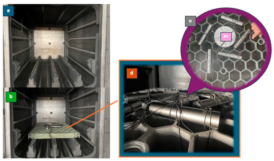
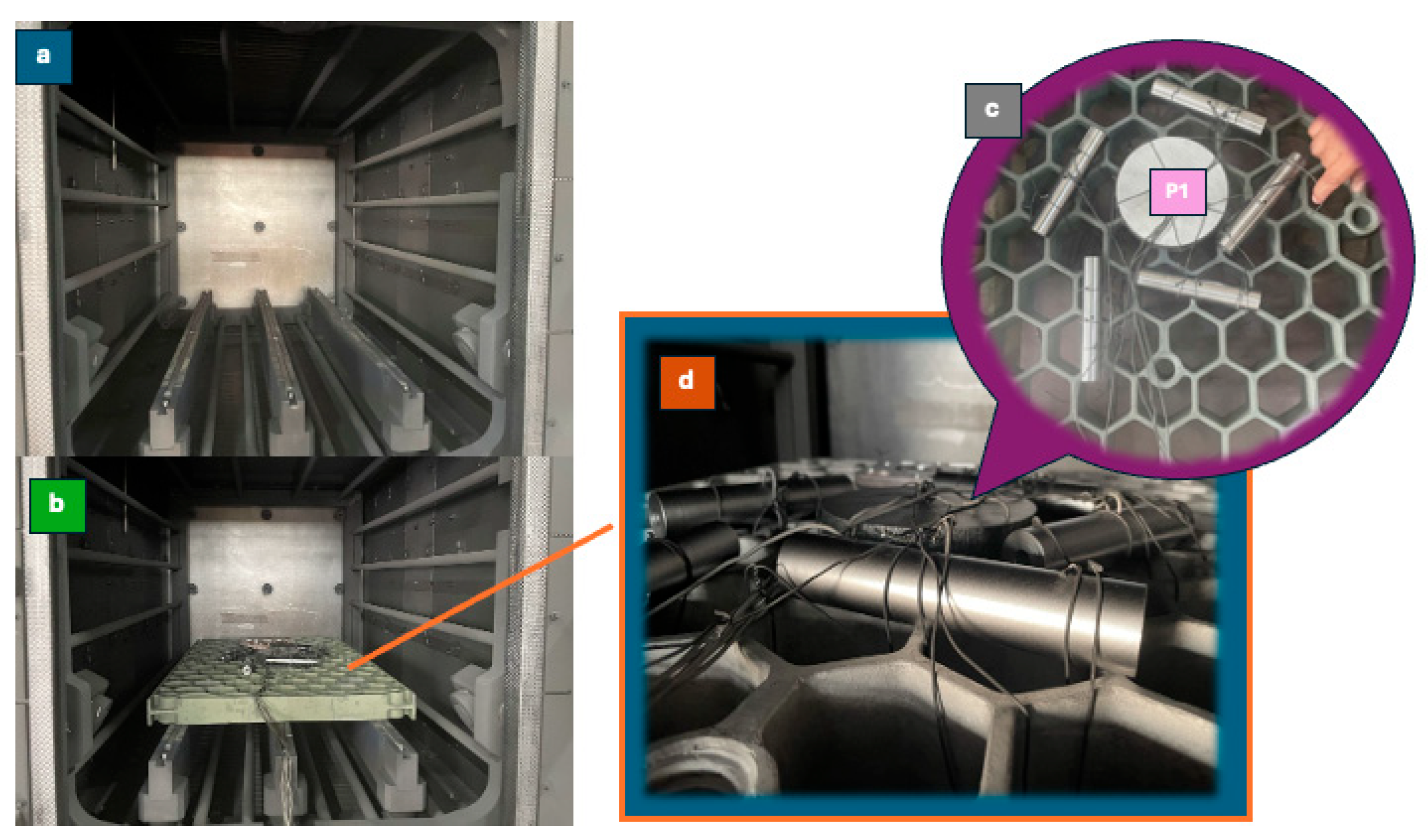
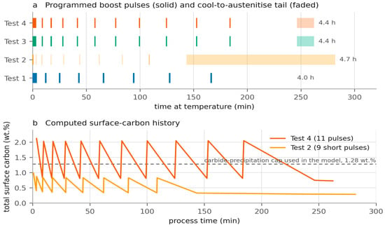
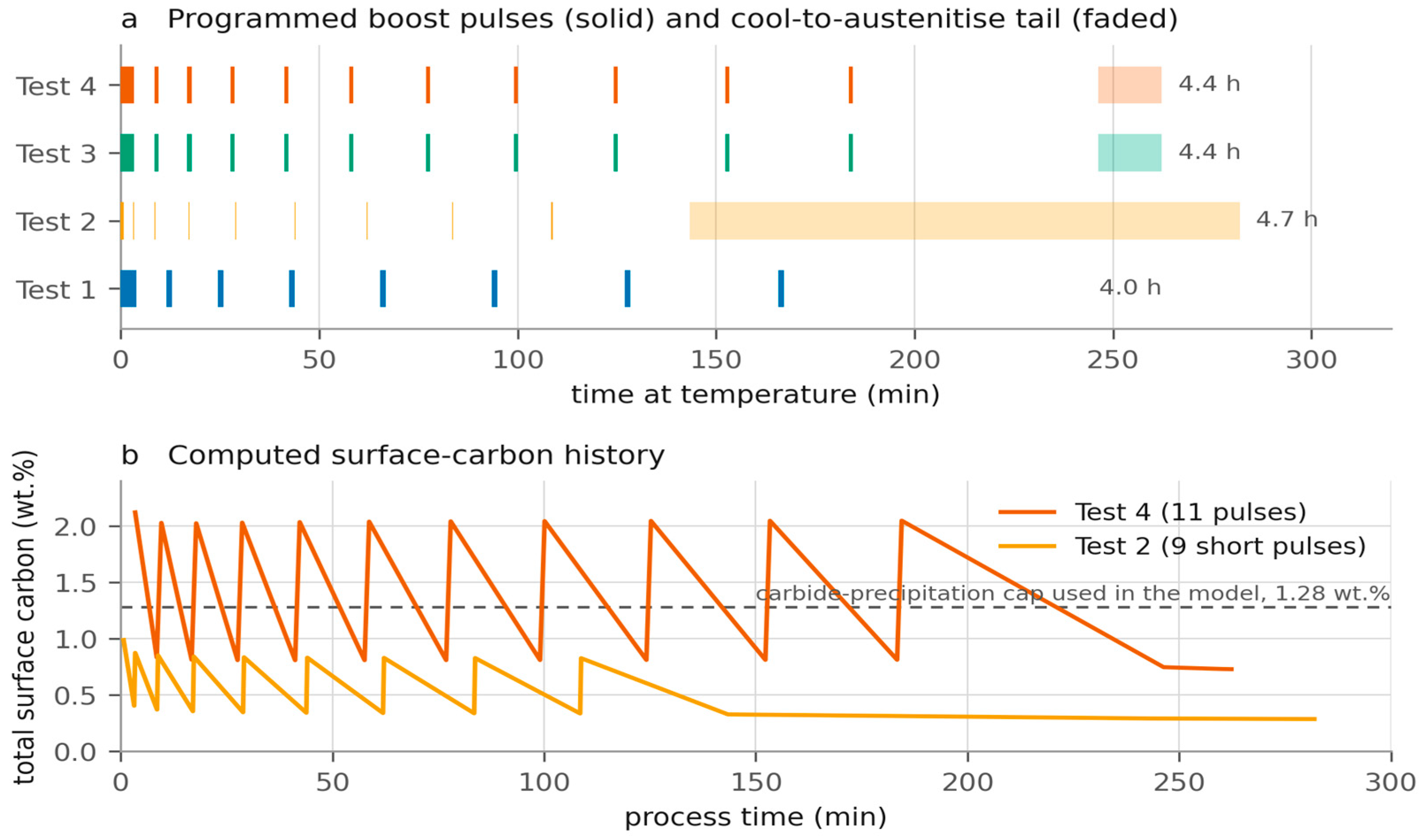
Four trials were run between April and July 2026 in a production vacuum furnace (Figure 1) with a 600 × 900 × 600 mm hot zone rated 300–1300 °C, capable of 10 bar N2 and 16 bar H2 gas quenching, with a base pressure observed to 2.0 × 10⁻² mbar. Loads were mixed-grade cylinder sets; the total exposed surface area and mass of each load are given in Table 1. All boosts were run at a 5-mbar partial-pressure set-point. The four pulse trains are compared in Figure 2a.
Figure 1.
The campaign. (a) The graphite hot zone of the production vacuum furnace. (b) The charge in the hot zone before Test 4 (c) The instrumented charge before loading: each cylinder carries a thermocouple in a drilled blind bore, and the numbered positions were tracked through the run; position 1 (P1) is the 22MnCrMoB5 disc. (d) The specimens immediately after the 10 bar H2 quench.
Table 1.
Trial conditions as programmed on the furnace controller, load data and recorded consumption. Boost and diffusion columns give the number of pulses and the first/last durations; the full sequences are in the Supplementary Recipe File.
Figure 2.
(a) Programmed schedules of the four trials. Solid marks are acetylene boost pulses; the faded bar is the cool-to- austenitizing tail. (b) Computed total surface carbon for Tests 4 and 2. The sawtooth is the boost/diffusion alternation; the dashed line is the carbide-precipitation cap used in the model (1.28 wt.%, the Fe–C Acm of 1.35 wt.% at 940 °C reduced for carbide-forming elements).
The written specification for every trial was inherited from a 22MnCrMoB5 production part: case depth 0.9–1.1 mm at 550 HV, austenitic grain finer than ASTM 6, surface hardness 60–63 HRC (Tests 1 and 2) or 60–65 HRC (Tests 3 and 4), and no surface carbide or oxidation. The 16MnCr5 cylinders were therefore process witnesses carried through a recipe written for a different grade, which provides context for interpreting deviations from the specification.
Because of a fault in the controller’s recipe export, the quench-gas field reads H2 in all four printed recipes. Only Test 4 was in fact quenched with hydrogen; Tests 1, 2 and 3 were quenched with nitrogen. This was recorded in the campaign log and reflected in the consumption figures, which showed 58 nm3 of hydrogen for Test 4 and none for the others. In Test 4, the chamber reached 9750 mbar of H2 within 58 s, fell to 7200 mbar as the gas cooled, and was not topped up, and the load went from 870 °C to 60 °C in 310 s.
2.4. Metallography and Hardness
Tests 1, 2 and 4 were evaluated by Teknotest Mühendislik ve Laboratuvar Test Cihazları (Gebze, Kocaeli), accredited to TS EN ISO/IEC 17025:2017 under TÜRKAK registration AB-2002-T. The reports specify Vickers traverses to TS EN ISO 6507-1 [16] at HV0.3 and metallography after 2% initial immersion etching at 50× or 100×. Test 3 was evaluated at Yeditepe University on the wall of the thermocouple bore, also at HV0.3. This was a separate exploratory examination of an internal feature, not a matched repeat of the external -laboratory free-surface protocol. The campaign records do not document a prior comparative sampling plan or a reason for selecting different laboratories. The optical case-layer measurements comprise three positions at 50× on the Test 3 bore section and one position at 9.8× on the Test 1 free surface.
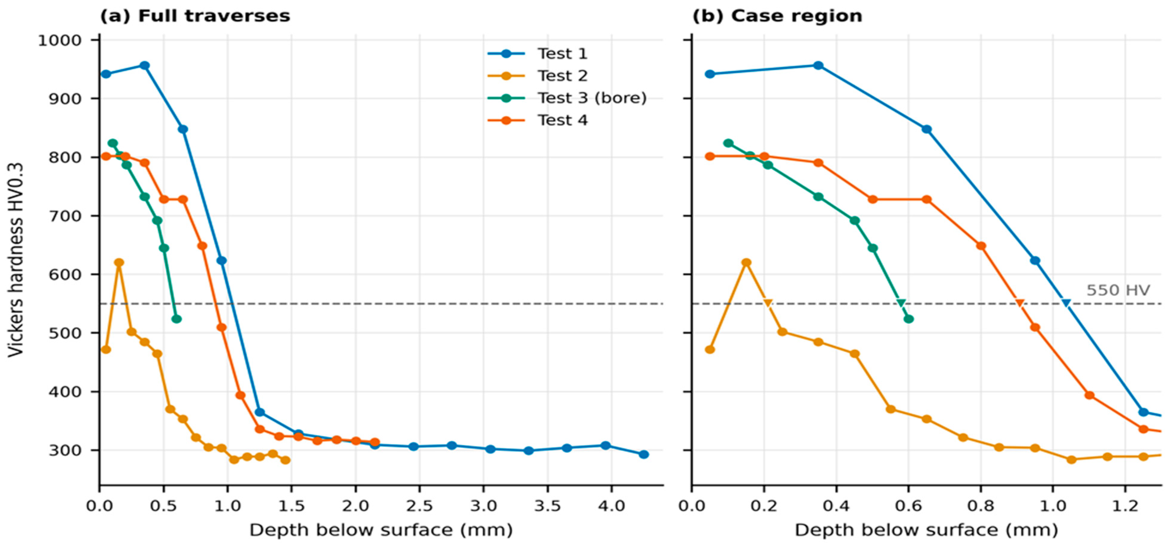
The measured quantity was denoted CHD550(HV0.3): the depth of the descending 550 HV crossing obtained by linear interpolation between adjacent indents. For depths z1 and z2 with H1 > 550 > H2, the interpolated depth was z1 + (H1 − 550)(z2 − z1)/(H1 − H2). The actual crossing brackets were 0.950–1.250 mm (Test 1), 0.150–0.250 mm (Test 2), 0.500–0.600 mm (Test 3) and 0.800–0.950 mm (Test 4). These sampling intervals constrained interpolation resolution but were not standard uncertainties. Replicate traverses, individual indentation uncertainty budgets and position-calibration uncertainties were unavailable; therefore, standard deviations or confidence intervals were not assigned to these depths.
HV0.3 was the load used in the archived testing, corresponding to approximately 2.94 N, compared with 9.81 N for HV1. The original reason for the chosen force and unequal spacing was not documented. A lower force samples a smaller microstructural volume and can be more sensitive to local constituents, preparation and in-dentation-size effects; no paired HV0.3/HV1 traverses established their magnitude or direction here. The 550 HV threshold was retained with reference to ISO 18203 [17], but these results were explicitly reported as CHD550(HV0.3), without claiming equivalence to an HV1 acceptance measurement. Replicated traverses at the required acceptance load and finer sampling near the crossing are needed for that purpose.
The model depth dC0.36 was the crossing of 0.36 wt.% C. This value is an inherited engineering comparison threshold, not a measured carbon–hardness calibration for this heat, and a primary calibration dataset establishing an exact 550 HV equivalence was unavailable. Its use was restricted to a provisional comparison for the present low-alloy steel and quench conditions. The empirical hardness-bridge depth dHV550 is reported separately in Section 3.7. Neither calculated depth was relabeled as a measured CHD550, and the criterion discrepancy is reported separately and is not interpreted as a measured carbon–hardness calibration or measurement uncertainty.
2.5. Model Formulation
Carbon transport in the case was treated as one-dimensional diffusion into a semi-infinite solid
with C the carbon concentration in wt.% and x the depth below the surface.
2.5.1. Diffusivity
The concentration- and temperature-dependent diffusivity of carbon in binary Fe–C austenite was taken from Ågren [11],
with yc = xc(1 − xc) and xc the carbon mole fraction. The alloy dependence was carried by a multiplicative composition factor kalloy of the Gunnarson type used by the industrial recipe engine,
which evaluates to 0.868 for the present heat, so that D = kalloy × DFe−C At 940 °C this gives 1.06 × 10⁻¹¹ m2 s−1 at the core carbon level, 1.49 × 10⁻¹¹ m2 s−1 at 0.5 wt.% C and 2.81 × 10⁻¹¹ m2 s−1 at 1.14 wt.% C. Section 3.4 shows that the placement of kalloy on the diffusivity rather than on the carbon activity is not decided by the present data.
kalloy = 1 + Si(0.15 + 0.033Si) − 0.0365Mn − Cr(0.13 − 0.0055Cr) + Ni(0.03 − 0.03365Ni) − Mo(0.025 − 0.01Mo) − Al(0.03 − 0.02Al)
2.5.2. Boost Boundary
During an acetylene pulse a constant carbon flux was imposed at the surface,
with J the kinetics-limited carbon uptake rate of the surface reaction. The pre-campaign value is the recipe engine’s carbon-transfer polynomial,
in mg h−1 cm−2 with T in °C, which gives 136.6 g C m−2 h−1 at 940 °C and 145.2 g C m−2 h−1 at 950 °C. A prescribed flux, rather than a prescribed surface concentration, is the physically appropriate boundary for LPC whenever the acetylene supply is in excess: the uptake is then limited by the surface reaction and by how fast the absorbed carbon can leave the surface, not by the gas [4,6]. Section 3.6 establishes that all four trials were in that regime by a factor of at least 49.
qC = −1.084 × 10⁻⁴T2 + 0.291T − 164.1
2.5.3. Diffusion Boundary
During a diffusion window, the acetylene was shut off, and the surface was treated as a zero-flux boundary, so the carbon already absorbed redistributed without loss. Decarburization into the residual vacuum atmosphere was neglected.
2.5.4. Cementite Reservoir
After each diffusion step, carbon above a nominal austenite saturation threshold was assigned to an immobile carbide reservoir, which redissolves when dissolved carbon falls below the threshold. The threshold followed the metastable Fe–C diagram [18,19] with an empirical alloy reduction. The reservoir capacity was 0.6 wt.% in the baseline calculation. If the reservoir is full, overflow is returned to dissolved carbon to conserve total carbon, so the algorithm did not enforce a strict dissolved-carbon cap in that state. This numerical treatment was not a resolved carbide-precipitation model. Section 3.1 examines its small influence on the checked case-depth criterion.
The programmed temperature schedule was integrated through the cool-to-austenitizing ramp and hold, using D(C,T) at each step. Test 2 included a 100 min ramp and a 38.5 min hold. Although the specimens were instrumented and a Test 4 quench summary was recorded, no time-resolved specimen-temperature histories for the carburizing and diffusion stages were available in the analysis archive. Programmed temperatures therefore served as proxies for specimen temperature. The ±10 °C study was a sensitivity scenario, not a measured temperature uncertainty; thermal lag and spatial gradients were unresolved.
2.5.5. What the Model Does Not Contain
There was no gas-phase chemistry, no soot or tar formation, no geometry other than a flat semi-infinite surface, no austenite grain growth, no quench kinetics, and no phase transformation. Hardness was therefore not a primary model output; where hardness is computed in Section 3.7, it is through an explicitly separate empirical bridge whose limitations are stated there.
2.6. Numerical Scheme and Verification
The equation is discretized by a semi-implicit finite-volume scheme on a uniform grid. Face diffusivities are the arithmetic mean of the adjacent nodal values; the diffusivity is updated by two Picard iterations per step, while the right-hand side is held at the old-time value, and the resulting tridiagonal system is solved directly. The surface node is a half-cell carrying the boundary flux; the far boundary is zero flux at 4000 µm, which is 2.6 times the deepest case reached anywhere in this study including the parameter sweeps; at that extreme, the concentration at the far boundary is still the core value to four decimal places.
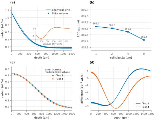
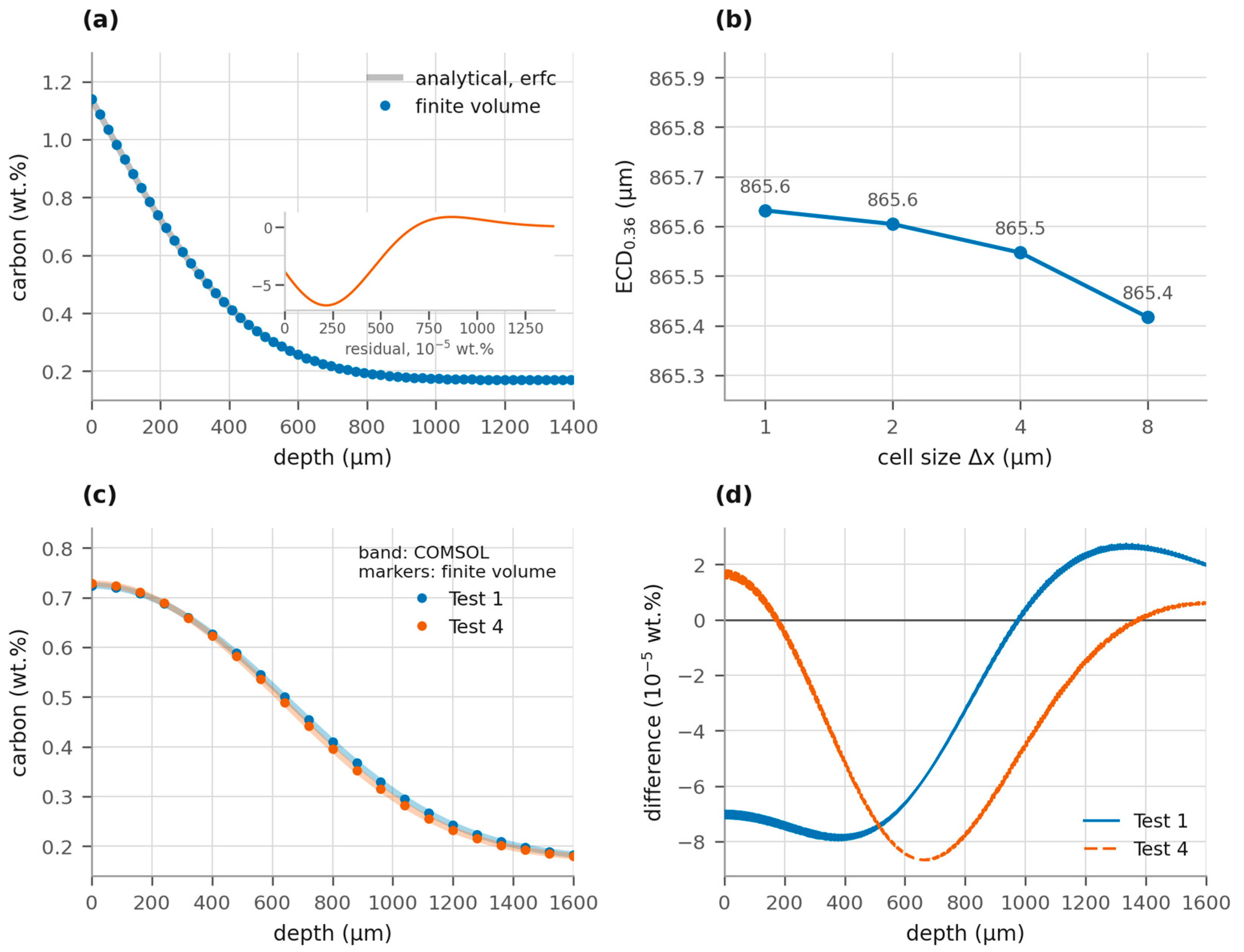
For numerical verification, the constant-surface, constant-diffusivity problem has the complementary-error-function solution in Equation (5). With D = 1.741 × 10⁻¹¹ m2 s−1 at 940 °C, Cs = 1.14 wt.%, C0 = 0.17 wt.% and t = 1 h, the scheme returns a 0.36 wt.% depth of 457.85 µm against the analytical 457.89 µm, analytically, a maximum concentration error of 6.8 × 10⁻⁵ wt.% and an RMS error of 2.0 × 10⁻⁵ wt.% (Figure 3a). This numerical benchmark is independent of experimental validation.
Figure 3.
Numerical verification. (a) Constant-surface, constant-diffusivity benchmark at 940 °C for 1 h. (b) Carbon-threshold depth for the full Test 4 schedule under coupled grid and time-step refinement. (c) Test 1 (eight boosts) and Test 4 (eleven boosts, with a non-isothermal tail), solved by finite volumes and COMSOL finite elements. (d) Concentration differences between implementations. Agreement verifies the selected equations and does not validate their material parameters.
A second, independent verification was run in COMSOL Multiphysics 6.4 through the LiveLink for MATLAB (R2010b) interface. The same problem—the same Ågren diffusivity with the same composition factor, the same prescribed-flux pulse train, the same zero-flux diffusion windows, and the same non-isothermal tail—was set up as a one-dimensional Transport of Diluted Species model on a graded mesh of 1600 elements with a 60:1 refinement towards the carburized surface, solved with a BDF scheme forced to step on every pulse edge. This is not a repeat of the finite-volume code: the discretization (Galerkin finite elements against finite volumes), the time integrator and the implementation were all different, so agreement cross-checks independent numerical implementations of the common equations. The COMSOL model conserves the imposed carbon to within 0.012% of the exact J·tboost budget for both schedules. Because the carbide reservoir is not implemented in COMSOL, the comparison was run against the finite-volume model with its cap removed, which Section 3.1 shows changes the result by 0.4 µm.
Grid convergence was checked on the full Test 4 schedule at Δx = 8, 4, 2 and 1 µm with the time step scaled proportionally. The effective case depth changed from 865.42 µm to 865.63 µm across that range, a spread of 0.025% (Figure 3b), and Δx = 4 µm with Δt = 4 s in diffusion windows and 0.5 s in boost pulses was used for subsequent baseline runs unless a refinement is stated.
2.7. Inverse Recipe Design
The original inverse recipe designer returned a temperature and boost–diffuse pulse train from target case-depth and surface-property inputs. Its output for Tests 3 and 4 was recorded before processing and is reproduced in Table 2. The predicted final depth was 1.1371 mm after the eleven boost–diffuse cycles. The programmed pulse durations agreed with this design record to the controller display resolution. This established the provenance of the historical recipe prediction; it did not establish that every numerical setting or subsequent thermal segment of the revised forward model was identical to the historical design engine.
Table 2.
Recipe designer output recorded before Tests 3 and 4, with the durations subsequently programmed on the controller. The designer’s own predicted depth after the final cycle was 1.1371 mm.
The historical engine used a prescribed boost-surface concentration from design solubility, giving 1.58 wt.% at 940 °C and 1.70 wt.% at 950 °C. The revised model used a prescribed uptake flux and a separate carbide-saturation treatment. The retained design table did not independently document the historical mesh, time-step policy, nonlinear solver, carbide treatment or inclusion of the cool-to-austenitizing tail. Thus, the archived 1137 µm prediction is a historical comparator, not an otherwise identical boundary-only control. A separate controlled numerical comparison, using common settings, is reported in Section 3.3.
2.8. Calibration and Identifiability Protocol
Two scalar multipliers were considered: ϕ on boost flux and λ on diffusivity, both unity in the uncalibrated model. A single multiplier was fitted at a time by minimizing squared log-depth residuals for Tests 1 and 4; leave-one-out transfer fit one trial and evaluated the other. A 9 × 9 parameter map was supplemented by a local log-sensitivity matrix S, with entries describing the change in log depth per change in log ϕ or log λ. Central perturbations of ±0.01 and ±0.02 in log parameter were used at the uncalibrated and flux-fitted points, and singular-value decomposition measured near-collinearity. Grid/time refinement checked numerical sensitivity. Without a measured observation-error covariance, the analysis was an unweighted conditioning diagnostic, not a statistical parameter-confidence calculation.
3. Results
3.1. Numerical Verification and Internal Sensitivity
The scheme reproduced the analytical benchmark within the errors reported in Section 2.6. Coupled spatial and temporal refinement changed the full Test 4 carbon-threshold depth by 0.025% (Figure 3b). This established a small discretization sensitivity for the checked formulation and schedules, without resolving constitutive or experimental uncertainty.
The independent COMSOL implementation and finite-volume code agreed closely for the common no-cap formulation (Figure 3c,d): the Test 1 depths were 894.30 and 894.33 µm, and the Test 3/4 depths were 865.87 and 866.00 µm. The maximum concentration difference was 8.7 × 10⁻⁵ wt.%, and the RMS difference was at most 3.3 × 10⁻⁵ wt.%. These checks supported the numerical consistency of the shared equations. They did not exclude common model-form errors or errors in input data.
The checked case-depth criterion was weakly sensitive to the reservoir treatment. Varying capacity from 0.1 to 3.0 wt.% changed the Test 4 depth from 865.8 to 865.3 µm; removing the threshold entirely gave 865.9 µm, and substituting the engine’s empirical carbide limit gave 864.8 µm. The prescribed boundary fixed the carbon budget, while the reservoir mainly affected the near-surface distribution. Total surface carbon exceeded the nominal dissolved-carbon threshold during pulses (Figure 2b), and reservoir overflow also exceeded that threshold in the dissolved field. The small depth sensitivity did not validate the calculated surface phase partition or carbide morphology.
Sensitivity to the temperature set-point was 6.1% of case depth per 10 °C: shifting the whole Test 4 schedule by ±10 °C moved the predicted depth from 866 µm to 813 µm and 918 µm. The cool-to-austenitizing tail of Tests 3 and 4 contributed 15 µm, that was 1.8%, whereas the 138.5 min tail of Test 2 was a first-order part of that trial.
3.2. Measured Case Depths
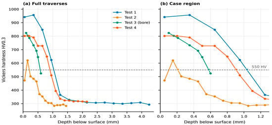
The measured traverses are given in Table 3 and plotted in Figure 4, and the sectioned specimens are shown in Figure 5. On free cylindrical surfaces, Test 1 gave CHD550 = 1036 µm with a surface hardness of 942 HV0.3 and a sub-surface maximum of 957 HV0.3 at 0.35 mm; Test 4 gave 907 µm with 802 HV0.3 at the surface. Both cores were 293–314 HV0.3. Inside the drilled bore, Test 3 gave 579 µm.
Table 3.
Vickers HV0.3 traverses on 16MnCr5. Tests 1, 2 and 4 were measured on the free cylindrical surface by Teknotest; Test 3 inside the drilled bore at Yeditepe University. Depth z in mm.
Figure 4.
Measured individual HV0.3 traverses: (a) full depth range and (b) case-region enlargement. Symbols are individual reported indentations; lines guide the eye. The dashed line is 550 HV and triangles mark the interpolated descending crossings. Test 3 is the bore traverse; the other tests are free-surface traverses. Repeatability data and measurement-uncertainty budgets are unavailable in the accessible numerical record, so statistical error bars are not assigned. Sampling brackets are reported separately in Table 4 and are not confidence intervals.
Figure 5.
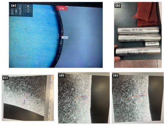
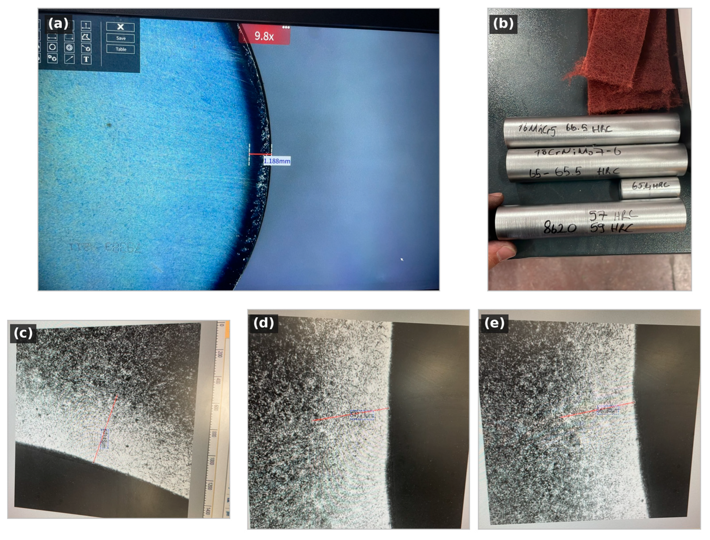
Available etched-layer and hardness records. (a) Test 1 free surface, 9.8×, with a calibrated segment of 1.188 mm. (b) Test 3 specimens with original HRC labels. (c–e) Three positions on one Test 3 bore section, 50×, with source measurements of 601.43, 543.73 and 567.30 µm. Original red measurement segments are retained and their values repeated below the panels. Panels (a,c–e) reproduce photographed displays, not native calibrated micrograph exports. The Test 3 display calibration belongs to the microscope image and cannot provide a reliable global scale bar on the oblique camera photograph. Native calibrated exports and high-magnification surface images are unavailable in the accessible archive.
Optical layer thickness and CHD550 are different observables. The three positions on the single Test 3 bore section gave a mean etched-layer thickness of 571 µm with a sample standard deviation of 29 µm, close to the 579 µm hardness crossing. These positions were not independent process replicates, and their scatter was not the uncertainty of CHD550. The single Test 1 optical thickness of 1.188 mm was 15% greater than its hardness crossing. Etch contrast did not establish a universal carbon or hardness threshold; only the hardness crossing was used as the measured comparator.
If the two measured hardness values correctly bracket 550 HV and the intervening profile is continuous and decreasing, the crossing lies within the sampling bracket [a,b]. For a fixed model depth p, the residual 100(p/d − 1) then spans 100(p/b − 1) to 100(p/a − 1). Unknown measurement bias can invalidate this conditional bracket. For the fixed joint-fit depths, the corresponding ranges were −21.2 to +3.7% (Test 1) and +0.4 to +19.2% (Test 4); these did not propagate uncertainty through the fitted parameter.
Table 4.
Sampling brackets and their conditional effect on uncalibrated residuals. Brackets are not confidence intervals; model depths are held fixed.
A complete uncertainty calculation would use the interpolation gradient g with respect to the two hardness values and two indentation positions, and their measurement covariance Σ, giving u2(d) = gΣgᵀ. For a fixed model depth, u(e) = 100p·u(d)/d2. The required covariance and systematic-error information were unavailable. The supplement provides the derivatives so these quantities can be evaluated when the laboratory uncertainty data are obtained; no numerical standard uncertainty is assigned retrospectively.
Test 2 had a non-monotonic near-surface traverse: 472 HV0.3 at 0.05 mm, 621 HV0.3 at 0.15 mm and 502 HV0.3 at 0.25 mm. The recorded data were retained without smoothing. A local microstructural gradient, retained-austenite variation, preparation or edge effects, or indentation scatter could contribute, but the available single traverse and low-magnification metallography do not distinguish these explanations. No carbon profile or retained-austenite measurement confirms a mechanism. The outermost layer was below 550 HV, so the descending crossing should not be interpreted as proof of a continuously hardened surface case.
The Test 3 bulk surface hardness of 66.5 HRC exceeded the specified 60–65 HRC band. This observation warrants a surface-microstructure investigation; hardness alone does not demonstrate excess dissolved carbon, grain-boundary carbide precipitation or retained-austenite content.
3.3. Uncalibrated Comparison and Boundary-Condition Controls
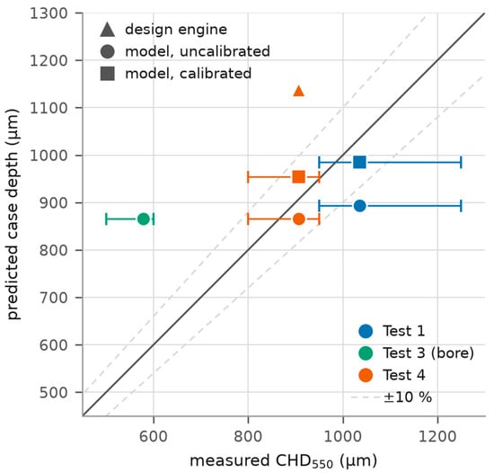
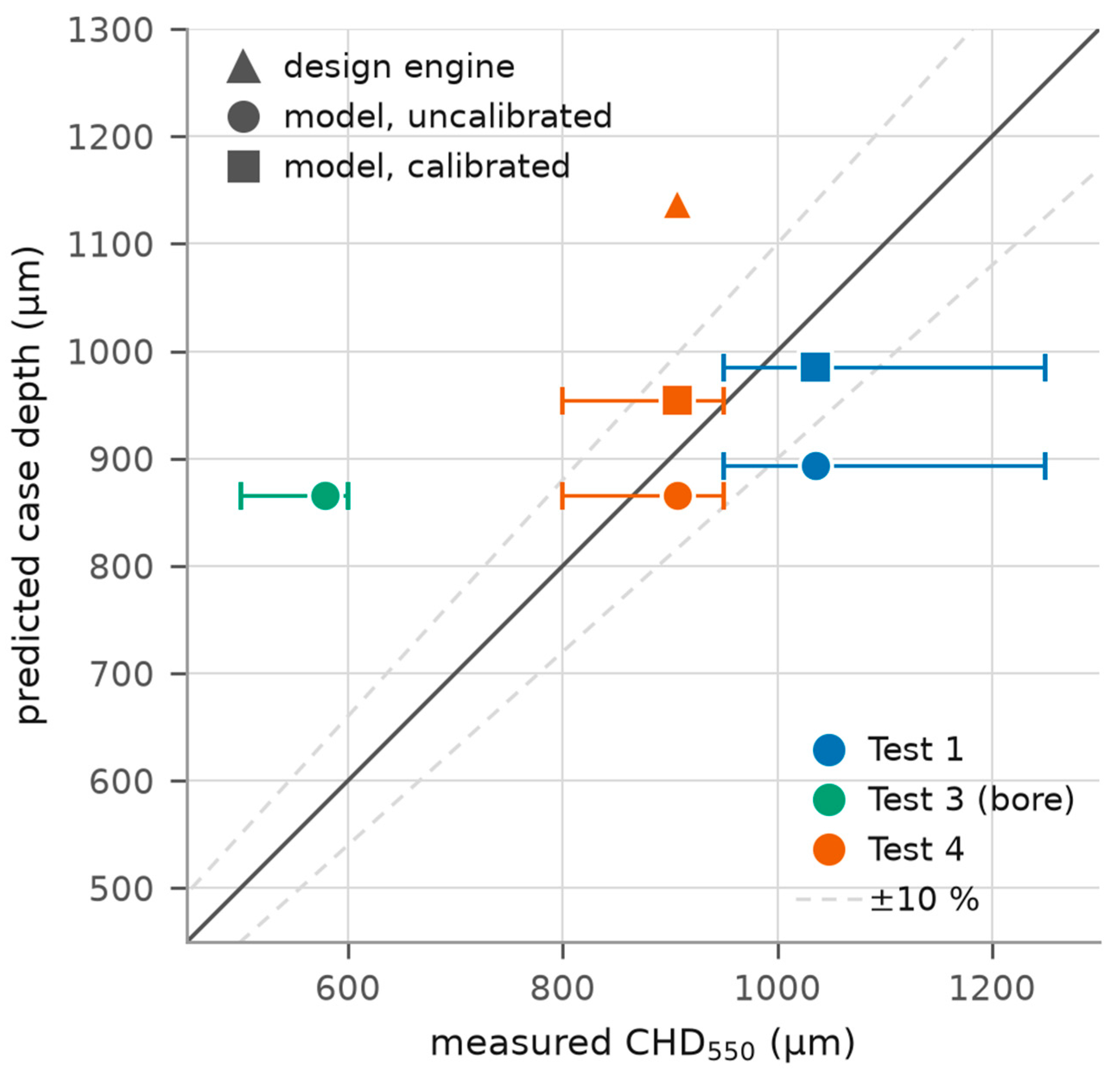
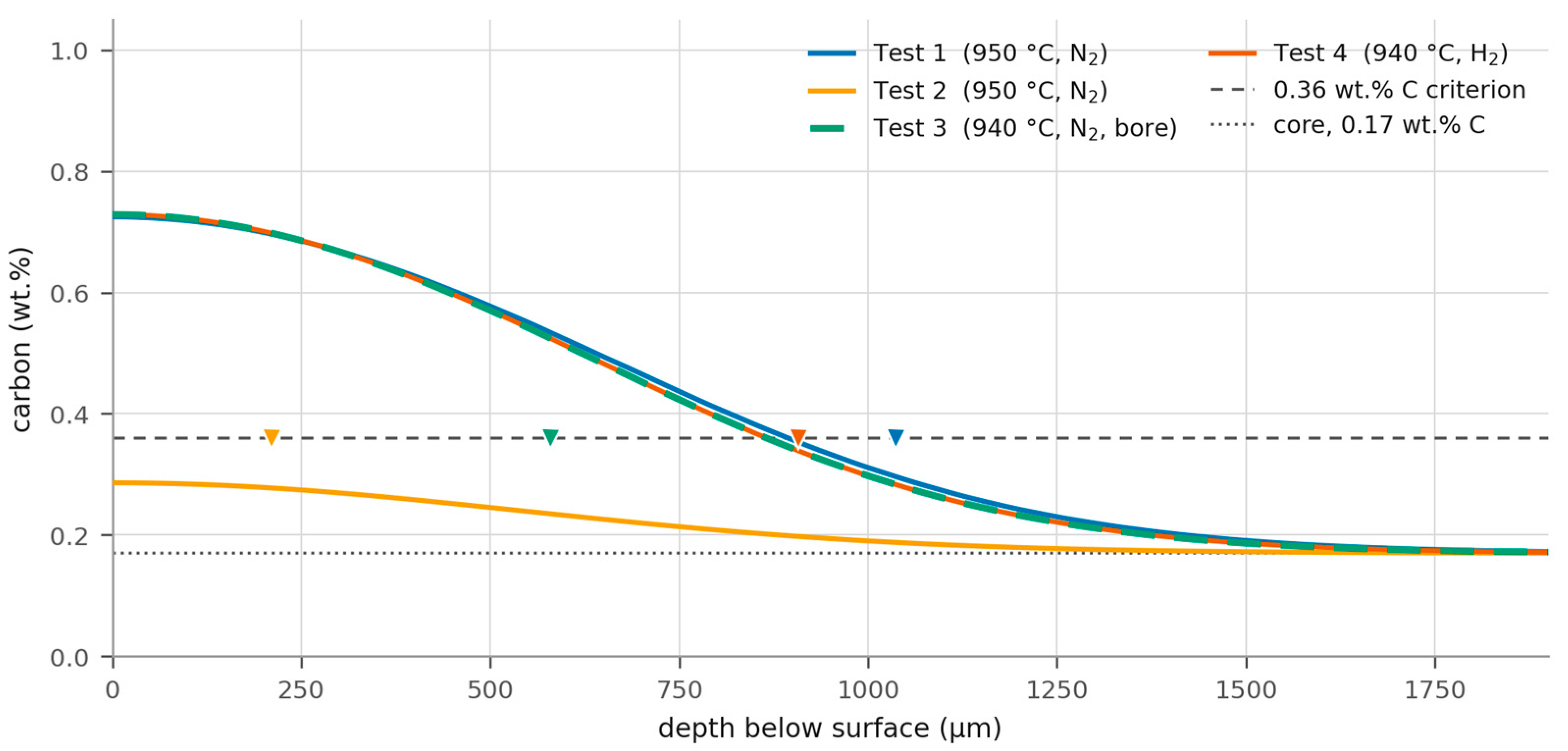
Figure 6 and Figure 7 compare uncalibrated carbon-threshold depths with the two measured free-surface hardness depths. The point deviations were −13.7% (Test 1) and −4.6% (Test 4), giving a two-observation mean absolute deviation of 9.1%. These describe the present comparisons conditional on the 0.36 wt.% criterion; they are not confidence bounds, an uncertainty budget or an estimate of performance on an industrial population (as show in Table 5 and Table 6).
Figure 6.
Calculated dC0.36 against measured CHD550(HV0.3). The historical designer output, uncalibrated model and joint fit are distinguished. Horizontal bars show the sampling brackets of the hardness crossings, not statistical error bars. Dashed ±10% lines are visual guides and do not represent a validated accuracy band. The bore observation is shown for context and excluded from free-surface calibration.
Figure 7.
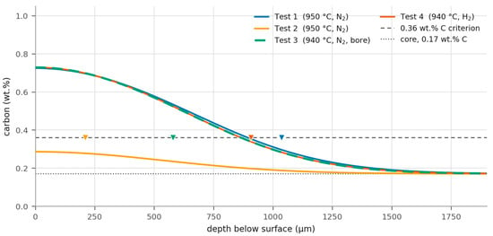
Uncalibrated carbon profiles. Measured hardness-depth markers are placed on the assumed 0.36 wt.% comparison line for visual comparison; they are not carbon measurements. Tests 3 and 4 have the same modelled thermal/pulse schedule and hence the same calculated profile, while their measured locations, loads, quench gases and laboratories differ.
Table 5.
Measured CHD550(HV0.3) and calculated dC0.36. The historical design output is from Table 2. Uncalibrated parameters are inherited without a fit to this campaign; the calibrated calculation uses ϕ = 1.213 fitted jointly to Tests 1 and 4. Deviations use interpolated measured point estimates and exclude measurement and criterion uncertainty.
Table 6.
Nominal supply and model uptake accounting. Supply is calculated from set-points, pulse durations and load area. Absorbed carbon is a model estimate, not a weighed uptake measurement. Estimated uptake/feed fractions are conditional on the gas-volume conversion, load representation and transfer law. The cylinder-weighing discrepancy is reported separately.
For Test 4, the historical 1137 µm design value had a +25.4% deviation, while the uncalibrated flux calculation had a −4.6% deviation. This was an improvement for that archived comparison, but the historical implementation was incompletely documented and could not identify the boost boundary as its sole cause. Nor could two free-surface observations establish that a flux boundary was consistently superior across steels, temperatures, surface states or gas-supply regimes.
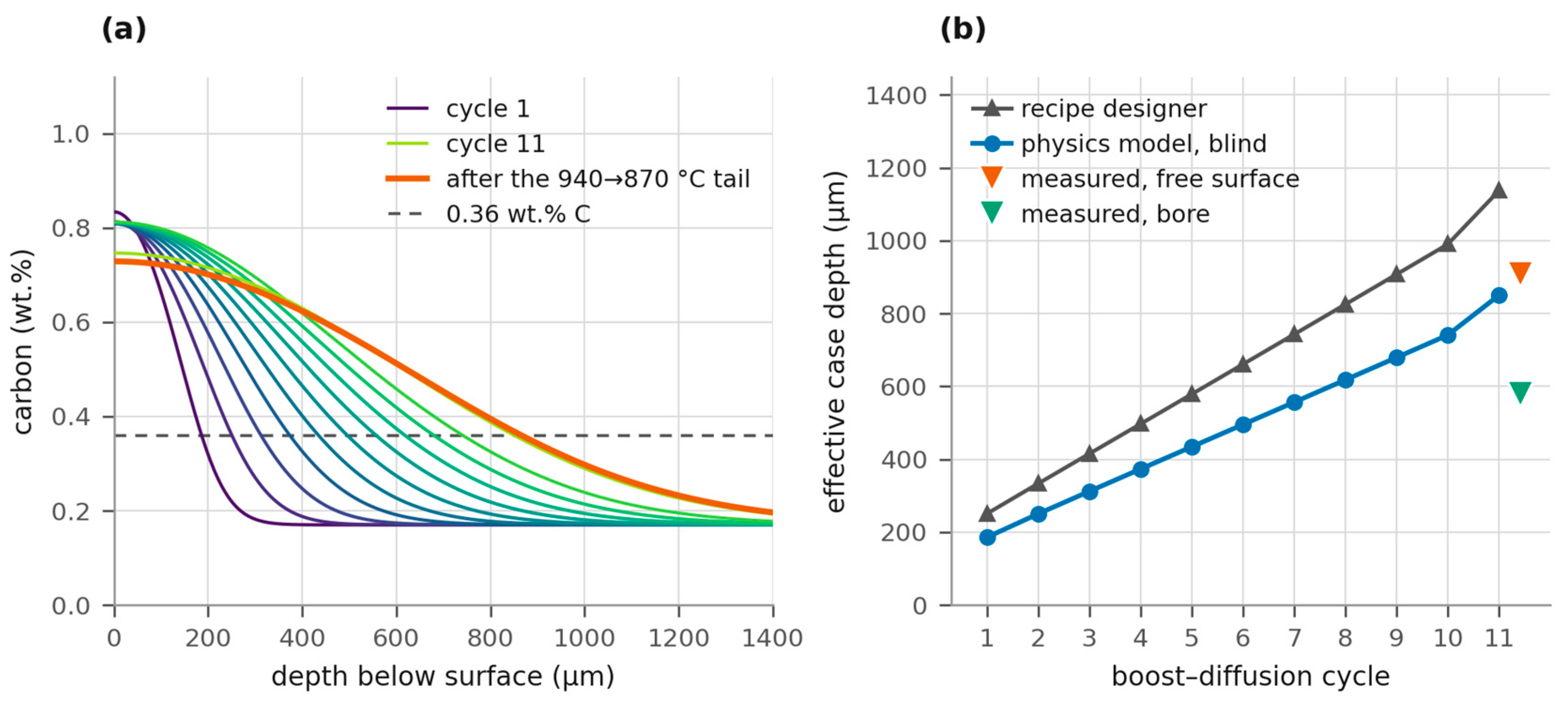
Figure 8 preserves the recorded cycle-by-cycle designer depths alongside the revised flux calculation. Their ratio remained approximately 1.31–1.34 during the pulse train. This described how the two calculations diverge; a near-constant depth ratio did not uniquely identify a boundary-condition error because changes in diffusivity can also produce approximately scaled depths.
Figure 8.
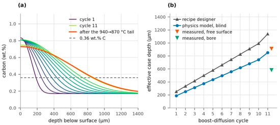
How the case is built. (a) Computed carbon profile after each of the eleven boost–diffusion cycles of the Test 3/4 recipe, dark to light, with the profile after the 940 → 870 °C tail in orange. (b) Effective case depth against cycle number for the pre-campaign recipe designer and for the physics model, with the two measured case depths at the end of the schedule. The two models stay in a constant ratio of 1.31–1.34 from the first cycle onwards.
Both concentration and flux boundaries responded to pulse duration. A fixed surface concentration supplied the flux needed to sustain its gradient, whereas the prescribed-flux model fixed the carbon budget per unit boost time. The earlier concentration-driven Robin calculation (β = 10−5 m s−1) fitted a surface potential of 1.686 wt.% and yielded about 615 µm for Test 2. That implementation also used the fitted potential as the carbide cap, so it was a coupled model-form comparison rather than a pure boundary-only test. The controlled comparison below separated the surface potential from the common carbide treatment. No version provided an experimental carbon-profile comparison for Test 2, and its measured nonzero hardness crossing must not be described as agreement with the absence of a calculated 0.36 wt.% crossing.
The new paired calculation kept D(C,T), kalloy, λ = 1, uniform initial carbon of 0.17 wt.%, zero initial carbide, the 0–4000 µm domain, 4 µm grid, 0.5 s boost/4 s diffusion steps, two Picard updates, full thermal schedule, zero-flux diffusion/far boundaries and the same 0.6 wt.% carbide-reservoir capacity. Only the boost rule changed: prescribed J(T) versus exact dissolved-carbon Dirichlet Csurface = Ccap(T). The latter was 1.3076 wt.% at 950 °C and 1.2780 wt.% at 940 °C; it was not the historical designer’s higher empirical solubility. Both arms used the same depth definitions and no fitted parameters given in Table 7.
Table 7.
Matched boost-boundary calculation, with all depths in µm. Carbon-threshold and empirical hardness-bridge depths are distinct. The planar model does not represent the Test 3 bore.
Under the carbon criterion, the flux arm was closer for Tests 1 and 4 (−13.7% and −4.6%) than the matched Dirichlet arm (−23.0% and −13.3%). With the empirical bridge, the Test 4 ranking was reversed: Dirichlet gave −1.7%, versus +6.3% for flux. Thus, the ranking depended on the comparison criterion. Test 2 had no flux-model crossing despite its nonzero hardness crossing, and neither planar arm validated the bore result. Halving the grid and time steps changed the matched Dirichlet Test 4 carbon depth by 0.089 µm (0.011%).
3.4. Calibration, Transfer, and What Case Depth Cannot Resolve
Fitting the single flux multiplier on both free-surface trials gave ϕ = 1.213 and reduced the deviations to −4.9% for Test 1 and +5.2% for Test 4. The residual was no longer a systematic underprediction; it was the two trials pulling in opposite directions, which is what a two-point fit of one parameter must produce when the two points are not exactly consistent.
In two-point leave-one-out transfer, fitting Test 1 gave ϕ = 1.353 and predicted Test 4 at 1003 µm (+10.6%); fitting Test 4 gave ϕ = 1.094 and predicted Test 1 at 936 µm (−9.6%). These two conditional transfer errors showed disagreement between the trial-specific calibrations. They did not define a ±11% prediction interval or establish reliable transfer to a new recipe.
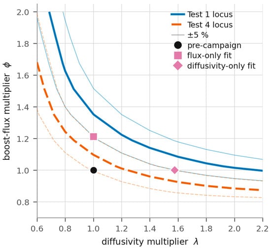
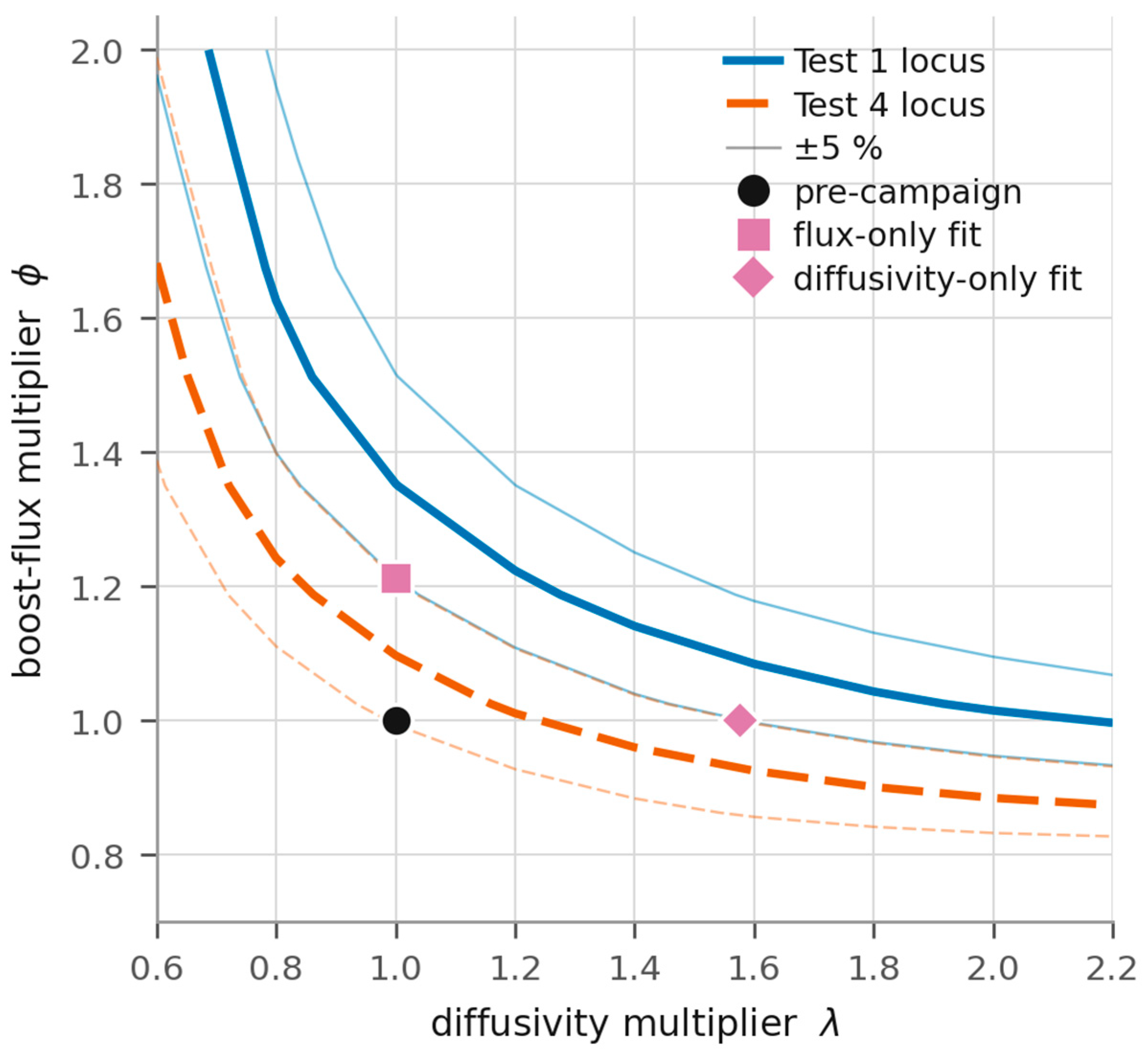
Alternatively fitting a diffusivity multiplier gave λ = 1.576 and nearly the same calculated depths as the flux fit: approximately 985 and 954 µm. The near-parallel depth loci in Figure 9 indicate poor practical separation of λ and ϕ for these schedules. This did not prove global structural non-identifiability for every possible experiment, nor did it show that Ågren diffusivity was physically wrong by 58%; unresolved surface transfer, temperature and criterion conversion contributed to the fitted multiplier.
Figure 9.
Depth-matching loci in the (λ, ϕ) plane for the two free-surface trials. Thin lines show ±5% depth bands used only as visual guides. The near-parallel loci suggest practical confounding for these schedules; the local sensitivity analysis provides a quantitative check. The two single-parameter fits are not independent measurements of either physical parameter.
The dimensionless local sensitivity coefficients for Tests 1 and 4 were almost equal (Table 8). At the uncalibrated point, the singular values of S were approximately 0.822 and 0.000263 on the base grid with a 0.01 log-parameter step. Across perturbation-size and grid checks, their ratio was approximately 3–4 × 10³; at the flux-fitted point it remained approximately 0.9–1.3 × 10³. The weak singular value was numerically delicate, but the severe near-collinearity was robust. This established practical ill-conditioning for the selected schedules and observable, not structural non-identifiability for all experiments.
Table 8.
Local log-depth sensitivities to flux and diffusivity multipliers. Base grid; central step 0.01 in log parameter. Values are derivatives, not experimental uncertainties.
A measured carbon profile would add observables with different sensitivities to flux and diffusivity, particularly near the surface. Suitable measurements include calibrated glow-discharge optical emission spectrometry or combustion analysis of serially removed layers, with depth and concentration uncertainty reported. Such data would improve parameter separation but would still require adequate resolution and a model-discrepancy assessment. More diverse pulse durations and temperatures can also improve identifiability; additional depth-only observations should be designed for sensitivity diversity rather than assumed to be uninformative in all circumstances.
3.5. Exploratory Bore Observation
For the same programmed pulse train and carburizing temperature, one bore traverse from Test 3 gave 579 µm, and one free-surface traverse from Test 4 gave 907 µm, a 36% cross-trial difference. The free-surface diffusion model gave the same 866 µm prediction for both schedules. This was a single-observation case study of a potential geometry effect, not an estimated general bore penalty or a within-specimen bore/free-surface contrast.
Fitting the bore traverse alone gave ϕbore = 0.552, approximately 45% of the joint free-surface fitted value. This coefficient describes the observed depth within the assumed one-dimensional model; it does not isolate gas transport or establish a design allowance. Restricted exchange of acetylene and reaction products in a blind cavity is one possible mechanism. Atmospheric gas-carburizing studies of bore size [20] provide qualitative motivation, but their material and gas conditions are not direct validation for the present LPC geometry.
The comparison also changed the load surface area (0.045 versus 0.145 m2), load composition and arrangement, quench gas (N2 versus H2) and evaluation laboratory. Because hardness depends on quench response as well as carbon uptake, these factors cannot be removed by normalizing gas flow to total load area. A larger nominal supply per unit area does not exclude local starvation, thermal differences or laboratory effects. Matched bore and external traverses on the same specimens, processed together and evaluated in one laboratory with replication, are needed before attributing the difference mainly to geometry.
A future bore model should couple gas-species transport in the cavity to carbon diffusion in the steel. A suitable continuum starting point is a transient convection–diffusion–reaction balance for acetylene and its products, with consumption at the steel wall tied stoichiometrically to the inward carbon flux and a pressure/composition boundary at the bore mouth. The measured bore dimensions, thermocouple occupancy, inlet history and wall kinetics would define the geometry and exchange time. A flow-regime check using the actual pressure, temperature and bore size is needed before choosing continuum or rarefied-gas transport. These inputs and matched measurements are unavailable here, so no validated physical bore simulation is claimed. Coupled reactive gas/solid modelling provides a published starting point [9], but its coefficients and geometry cannot be transferred without checking the present conditions. If the thermocouple occupies the bore during boosting, the annular clearance must be resolved and used in the local Knudsen-number check. The blind end has no normal gas velocity, but its steel surface still requires a reactive species boundary; this produces a spatially and temporally varying uptake flux rather than a universal scalar penalty.
3.6. The Gas-Supply Regime
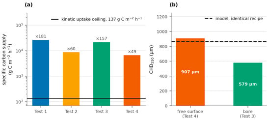
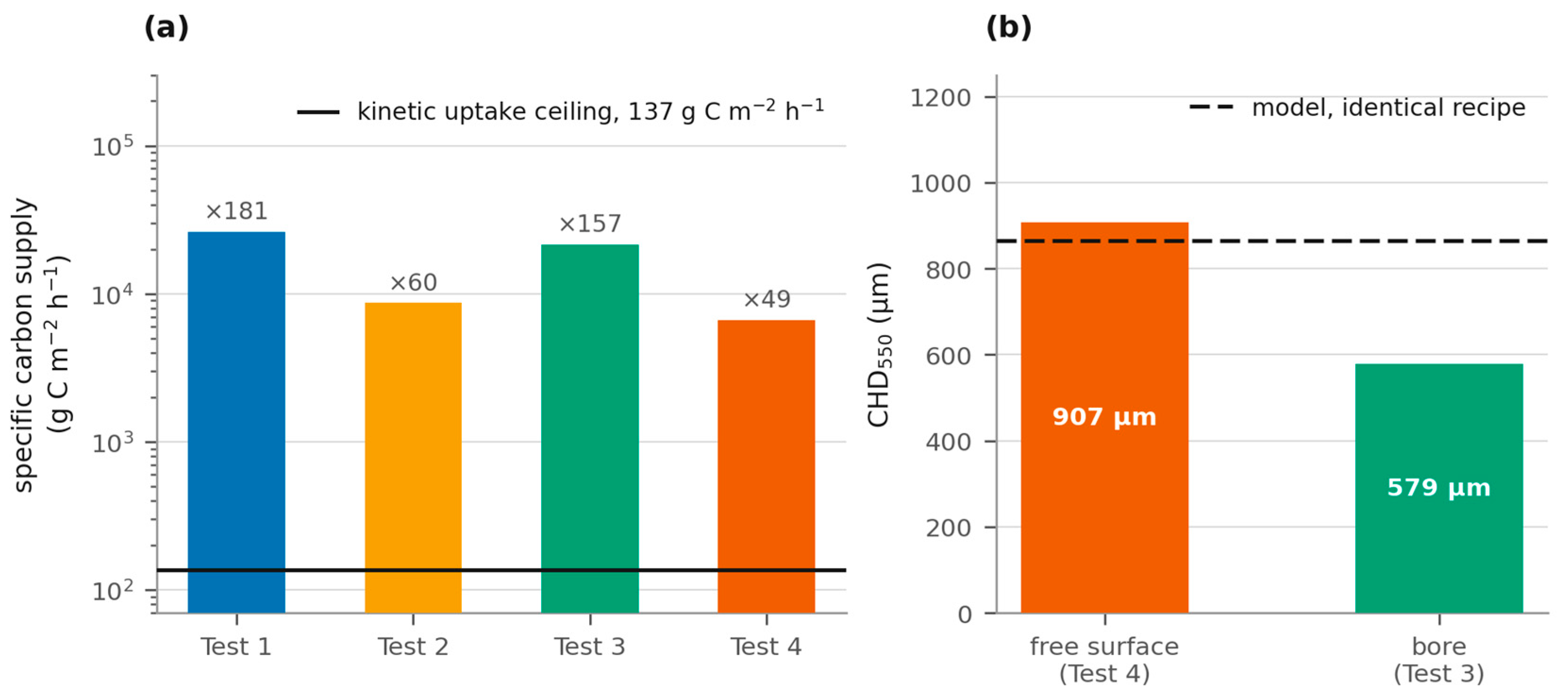
Table 8 and Figure 10 compare nominal carbon supply inferred from acetylene set-points with the assumed uptake rate. The resulting supply/uptake ratios are 49–181. Under the adopted unit conversion and uptake law these ratios suggest a globally abundant feed, but neither the actual carbon flux reaching each surface nor supply saturation inside the load is measured. The calculation therefore supports investigation of the prescribed-flux approximation in Section 2.5; it does not experimentally establish flow independence.
Figure 10.
(a) Nominal set-point carbon supply per unit load area compared with the assumed model uptake rate. (b) A bore traverse and a free-surface traverse from different trials using the same programmed recipe. The model prediction is shown for reference. Neither panel is a controlled experimental test of gas-flow independence or an isolated geometry effect.
Tests 3 and 4 did not provide two comparable free-surface results: Test 3 was evaluated only inside the bore. Their threefold difference in nominal specific supply therefore cannot be used as an independent demonstration that free-surface case depth is insensitive to flow.
The calculated uptake/feed fractions of 0.6–2.1% were conditional accounting quantities. Uptake was extrapolated across mixed-grade load area using the 16MnCr5 model, while gas supply was inferred from unverified flow settings. No measurement partitioned the remaining feed between unreacted gas, reaction products, soot or other losses. Accordingly, no measured transfer efficiency or quantified soot reduction was inferred from Table 8. Boost-only acetylene estimates were 0.60, 0.04, 0.25 and 0.25 kg, whereas cylinder weighing recorded 1.00, 0.40, 1.54 and 0.56 kg. The approximately 1.7–10-fold discrepancy was unresolved. The retained record did not specify whether weighing included line purging, manifold filling or chamber conditioning, nor did it provide their timing, duration or gas allocation. These are possible contributions, not a reconstructed purge protocol. The standard-volume reference conditions, flow-meter calibration and weighing window must be reconciled before a mass balance can be closed. Changing the denominator from nominal boost supply to weighed cylinder consumption would change the estimated uptake fraction substantially, without turning it into a measured transfer efficiency. The accessible controller recipes prescribe acetylene during boosts and zero acetylene during diffusion. They do not document separate line or manifold operations or define the cylinder-weighing accounting boundary. A purge contribution is therefore neither confirmed nor excluded by the printed boost–diffuse sequence.
3.7. Hardness: What the Model Does Not Predict
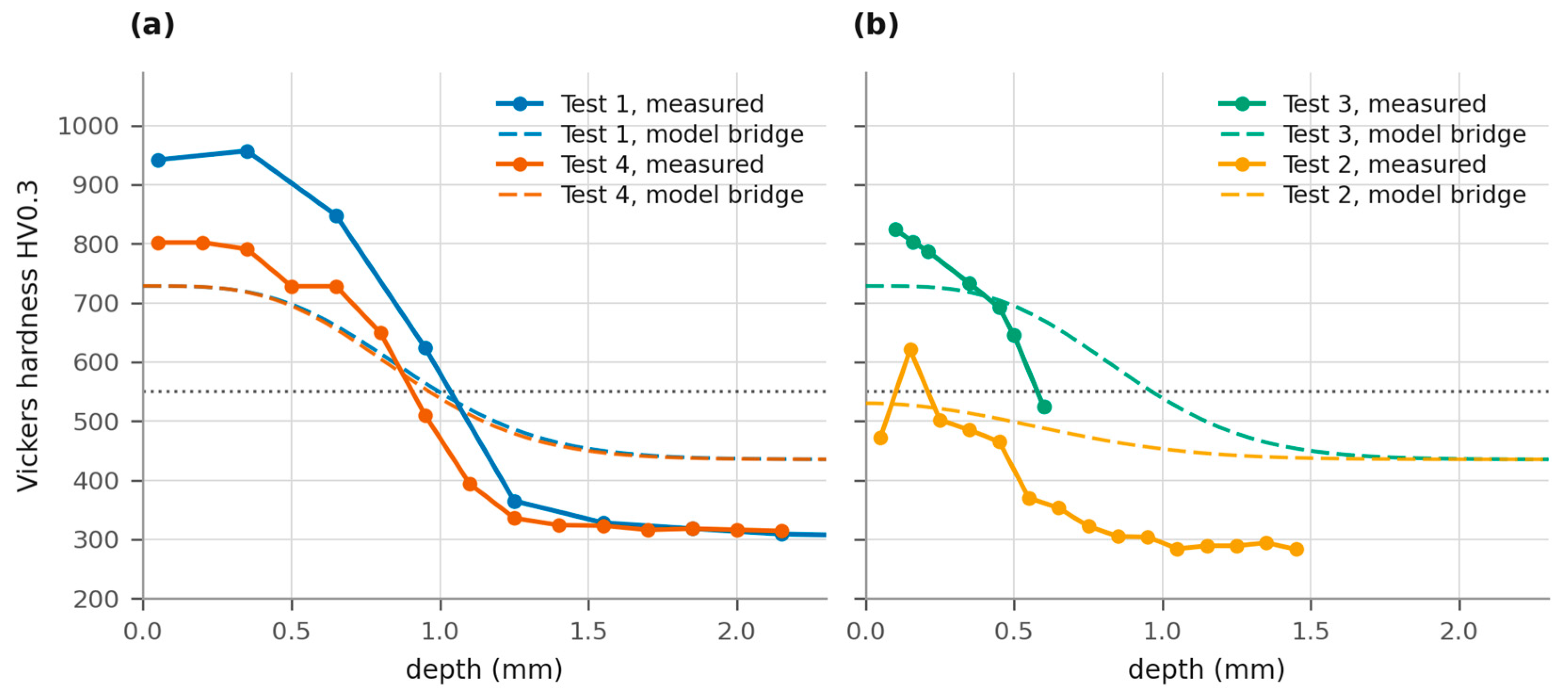
Figure 11 explores the assumed carbon–hardness link using a separate empirical bridge: Andrews’ martensite-start relation [21], the Koistinen–Marburger transformation relation [22] and the recipe engine’s saturating martensite-hardness curve. These ingredients did not constitute an experimental calibration for this heat or its gas-quench histories. The bridge was used as a criterion-sensitivity scenario, and the resulting dHV550 was distinguished from both dC0.36 and measured CHD550(HV0.3).
Figure 11.
Measured HV0.3 traverses and an empirical hardness bridge applied to uncalibrated carbon profiles. (a) Free surfaces. (b) The bore and under-carburized observations. The bridge is a model-based sensitivity scenario and is not independently validated by carbon, retained-austenite or phase-fraction measurements.
The bridge fails in three specific ways, all instructive.
Near the surface, it underpredicts; the bridge gave approximately 728 HV versus first-indent values of 802 HV in Test 4 and 942 HV in Test 1. This mismatch does not identify its cause. Grain-boundary carbides, retained austenite, local indentation effects and residual stresses cannot be confirmed or excluded from the available low-magnification images. In particular, high hardness alone is not evidence of carbide precipitation. No 500×–1000× surface micrographs for Tests 1 and 3, SEM phase analysis, retained-austenite measurements or residual-stress measurements are available in the retained dataset.
In the core, the bridge predicted about 435 HV against 293–314 HV measured. It assumes a predominantly martensitic response and omits the actual cooling history and competing transformation products. Incomplete hardening is a plausible explanation, but the carbon error and phase-transformation contribution cannot be separated without measured carbon and microstructure. A coupled thermal/transformation calculation would be needed to test the mechanism.
Re-evaluation of the archived profiles gave dHV550 = 995.5 µm for Test 1 and 963.7 µm for Test 4, compared with dC0.36 = 893.8 and 865.5 µm. The bridge mapped 550 HV to approximately 0.313 wt.% C for this composition, whereas it gave approximately 583 HV at 0.36 wt.% C. Thus, the bridge does not independently justify the inherited threshold. Table 9 separates both criteria and the corresponding deviations, including application to the existing flux fit without refitting. The approximately 11% uncalibrated depth shift is an alternative-model comparison, not a confidence limit; it is not included in the reported joint-fit or transfer errors and cannot be added in quadrature as though it were a measured standard uncertainty.
Table 9.
Separates both criteria and the corresponding deviations, including application to the existing flux fit without refitting.
3.8. The Under-Carburized Trial
Test 2 fell far below the target hardness-depth range. Its much shorter total boost duration and long cool-to-austenitizing tail were retained in the calculation, which gives surface carbon of 0.286 wt.% and no 0.36 wt.% crossing. The measured traverse nevertheless had a local maximum above 550 HV and a descending crossing near 210 µm. Therefore, the carbon-threshold calculation did not quantitatively reproduce this hardness-defined depth.
The model flagged this recipe as a candidate for inadequate carburizing under its stated criterion, which is useful for screening. The observation supports the need to examine the short-boost schedule, but it does not validate the predicted carbon profile or justify describing an absent calculated crossing as agreement with a measured nonzero crossing. Explaining the non-monotonic hardness requires additional microstructural or concentration evidence.
4. Discussion
4.1. What Has Been Established
The numerically verified model provides uncalibrated, criterion-conditional comparisons for two free-surface industrial observations, with point deviations of −13.7% and −4.6%. It can support preliminary recipe screening within the studied 16MnCr5 furnace conditions. The historical designer comparison, controlled boundary calculations, joint calibration and two-point transfer answer different questions and are reported separately. The campaign does not establish a general ±11–14% accuracy bound, consistent superiority of one boundary condition, or acceptance-grade case-depth prediction.
4.2. What Has Not Been Established
The following limitations define the experimental scope.
Absolute carbon: Absolute carbon is the primary experimental limitation. No GD-OES profile, serial-layer combustion analysis or other measured carbon profile is available. Consequently, the predicted surface values of 0.72–0.73 wt.% and the entire concentration profile remain unverified; evaluation is restricted to depth-criterion comparisons with an uncertain carbon–hardness link.
Surface microstructure and hardness: Near-surface and bulk hardness were measured, but the model does not quantitatively reproduce them. The available images do not confirm or exclude a grain-boundary carbide network. High-magnification optical/SEM examination would address carbide morphology; retained austenite and residual stress would require suitable phase- and stress-sensitive measurements. The present study cannot certify the no-carbide requirement.
Core properties: Core hardness was measured, but the model lacks the thermal and transformation physics needed to predict it. The hardness bridge overprediction is a model limitation rather than evidence of a uniquely identified carbon or hardenability error.
Geometry: The one bore observation is confounded by trial, load, quench and laboratory differences. The fitted bore multiplier is descriptive and cannot be transferred to blind holes, gear roots or internal corners without matched experimental and transport-model validation.
4.3. Identifiability as a Design Constraint on Future Experiments
The sensitivity analysis shows that these two similar schedules poorly separate flux from diffusivity. Replicating them would reduce some random experimental error but would not necessarily remove the near-collinearity. Carbon profiles, independently measured uptake and schedules chosen to generate different sensitivity directions would provide more informative constraints. Profile measurements on archived specimens, if available, would be particularly useful, alongside replicated free-surface and bore traverses with consistent testing protocols [8].
4.4. Process Implications
Three process ideas follow as testable inferences. First, the nominal supply calculation motivates stepwise acetylene-flow reduction trials with carbon profile, CHD, soot and flow-meter measurements; it does not specify a safe minimum flow or guarantee unchanged depth. Second, load area is a useful scaling variable, but mixed grades, packing, surface state and local transport must also be controlled. Third, complex features require paired geometry measurements and a transport model rather than applying the fitted bore multiplier as a recipe correction. Extrapolation to another furnace, steel, temperature, quench or load may change both uptake and the carbon–hardness relation, so the present calibration is not transferred without validation.
Published successful flow reduction [13] demonstrates feasibility under the conditions tested there, while measured pressure/flow effects [14] caution against extrapolating that result. These studies support controlled optimization rather than an unconditional recommendation to reduce the present set-points.
4.5. Limitations
Four trials include only two free-surface observations suitable for the present calibration. The two-point trans-fer errors are not a distribution, and no replicate process trials establish reproducibility. Measurement-force effects, coarse and unequal indentation spacing, an unvalidated carbon–hardness conversion, missing carbon profiles, mixed-grade loads and unavailable specimen-temperature histories all limit inference. The ±10 °C calculation is a sensitivity scenario; it cannot be combined with sampling brackets or criterion changes into a total statistical uncertainty without additional measurement information.
5. Conclusions
- The finite-volume formulation is verified against an analytical solution, coupled grid/time refinement and an independent COMSOL implementation of the common no-cap problem. Numerical agreement does not validate the material law or experimental comparison criterion.
- For two free surfaces, uncalibrated dC0.36 gives point deviations of −13.7% and −4.6% from CHD550(HV0.3). The absence of measured carbon profiles is the primary experimental limitation, and no general accuracy interval is inferred.
- The historical recipe-designer output has a +25.4% deviation for Test 4. Its incomplete numerical provenance prevents the attribution of the entire difference solely to the boost boundary. Controlled comparisons test boundary assumptions locally and do not establish universal superiority.
- A joint flux fit gives residuals of −4.9% and +5.2%; two-point transfer gives +10.6% and −9.6%. An empirical hardness bridge shifts uncalibrated depths by about 11%, separately from these residuals and from measurement uncertainty.
- Flux and diffusivity are poorly distinguishable from the two similar depth observations. Local sensitivity analysis supports practical confounding; measured profiles and experiments with more diverse sensitivities are needed for stronger parameter identification.
- Nominal supply/uptake ratios of 49–181 and calculated uptake/feed fractions are conditional model estimates. Disagreement with cylinder weighing prevents a measured transfer-efficiency claim and motivates calibrated gas accounting before flow-reduction trials.
- The 36% bore/free-surface difference is one cross-trial observation with load, quench and laboratory confounds. The effective bore multiplier is not a validated geometry correction.
- Surface and core hardness were measured but are not validated model outputs. The available metallography does not establish carbide, retained-austenite or residual-stress explanations; the model remains unvalidated for absolute carbon profiles and complex internal geometries.
Supplementary Materials
The following supporting information can be downloaded at: https://www.mdpi.com/article/10.3390/jmmp10110457/s1. The original solver, recipe definitions, profile outputs and verification files are retained with the revision supplement. The additions reviewer_numerics.py and refine_sensitivity.py reproduce the sampling-bracket calculations, criterion comparison, controlled boundary calculation and local sensitivity analysis; their numerical results and a reproducibility note are included.
Author Contributions
Conceptualization, M.B.D. and H.İ.Y.; methodology, M.B.D.; software, M.B.D.; validation, M.B.D. and H.İ.Y.; formal analysis, M.B.D.; investigation, H.İ.Y. and M.B.D.; resource, H.İ.Y. data curation, M.B.D.; writing—original draft preparation, M.B.D.; writing—review and editing, H.İ.Y. and M.B.D.; visualization, M.B.D.; supervision, H.İ.Y.; project administration, H.İ.Y. All authors have read and agreed to the published version of the manuscript.
Funding
This research received no external funding.
Data Availability Statement
All results reported in Section 3.1, Section 3.2, Section 3.3, Section 3.4, Section 3.5, Section 3.6, Section 3.7 and Section 3.8 are reproduced by running fi-nal_analysis.py, extra.py, cycles.py and robin_check.py, followed by figures.py, fig03.py and figures_new.py; the independent finite-element cross-verification is com-sol/LPC_16MnCr5_COMSOL_both.m, which runs against COMSOL Multiphysics 6.4 through Live-Link for MATLAB and writes the profiles compared by comsol_compare.py. No random number is used anywhere in the analysis, so every value is deterministic. The experimental records transcribed into recipes.py—controller recipe screens, load sheets, consumption records, accredited test reports and the material certificate—are listed with their provenance in campaign_records.md. The original records are held by the authors and by Sistem Teknik Sanayi Fırınları A.Ş. and are available from the corresponding author on reasonable request.
Acknowledgments
The trials were carried out at Sistem Teknik Sanayi Fırınları A.Ş., Çayırova, Kocaeli. Hardness and microstructure testing for Tests 1, 2 and 4 was performed by Teknotest Mühendislik ve Laboratuvar Test Cihazları San. ve Tic. Ltd. Şti., Gebze, Kocaeli, accredited by TÜRKAK under registration AB-2002-T. The authors acknowledge Yeditepe University for providing the computationXal infrastructure that supported this research.
Conflicts of Interest
The remaining authors declare no conflicts of interest. The company had no role in the design of the model, in the analysis or interpretation of the data, or in the decision to publish the results.
Abbreviations and Standarts
The following abbreviations and standarts are used in this manuscript:
| EN 10204 | European Standard EN 10204 |
| ISO 643 | International Standard ISO 643 (Steels—Micrographic determination of the apparent grain size |
| HB | Brinell hardness (HB) |
| TS EN ISO/IEC 17025:2017 (TÜRKAK AB-2002-T) | General requirements for the competence of testing and calibration laboratories) under the Turkish Accreditation Agency |
References
- Gorockiewicz, R. The kinetics of low-pressure carburizing of alloy steels. Vacuum 2011, 86, 448–451. [Google Scholar] [CrossRef] [Scilit]
- Iżowski, B.; Wojtyczka, A.; Motyka, M. Numerical simulation of low-pressure carburizing and gas quenching for Pyrowear 53 steel. Metals 2023, 13, 371. [Google Scholar] [CrossRef] [Scilit]
- Viliš, J.; Dobrocký, D.; Joska, Z.; Procházka, J.; Klimeš, M. The effect of changing the temperature of the vacuum carburizing process on the layer properties of steels used in the automotive industry. Int. J. Adv. Manuf. Technol. 2025, 137, 2823–2833. [Google Scholar] [CrossRef] [Scilit]
- Wang, H.; Liu, J.; Tian, Y.; Wang, Z.; An, X. Mathematical modeling of carbon flux parameters for low-pressure vacuum carburizing with medium-high alloy steel. Coatings 2020, 10, 1075. [Google Scholar] [CrossRef] [Scilit]
- Zajusz, M.; Tkacz-Śmiech, K.; Danielewski, M. Modeling of vacuum pulse carburizing of steel. Surf. Coat. Technol. 2014, 258, 646–651. [Google Scholar] [CrossRef] [Scilit]
- Guo, J.; Deng, X.; Wang, H.; Zhou, L.; Xu, Y.; Ju, D. Modeling and simulation of vacuum low pressure carburizing process in gear steel. Coatings 2021, 11, 1003. [Google Scholar] [CrossRef] [Scilit]
- Buchholz, D.; Khan, R.U.; Bajohr, S.; Reimert, R. Computational fluid dynamics modeling of acetylene pyrolysis for vacuum carburizing of steel. Ind. Eng. Chem. Res. 2010, 49, 1130–1137. [Google Scholar] [CrossRef] [Scilit]
- Atraszkiewicz, R.P.; Dybowski, K. Minimizing deformations in high-temperature vacuum carburizing. Materials 2023, 16, 7630. [Google Scholar] [CrossRef] [Scilit] [PubMed]
- Yada, K.; Watanabe, O. Reactive flow simulation of vacuum carburizing by acetylene gas. Comput. Fluids 2013, 79, 65–76. [Google Scholar] [CrossRef] [Scilit]
- Tapar, O.B.; Epp, J.; Steinbacher, M.; Gibmeier, J. In-situ synchrotron X-ray diffraction investigation of micro-structural evolutions during low-pressure carburizing. Metall. Mater. Trans. A 2021, 52, 1427–1442. [Google Scholar] [CrossRef] [Scilit]
- Ikehata, H.; Tanaka, K.; Takamiya, H.; Mizuno, H. Effect of chemical compositions of case hardening steels for distribution of carbon and cementite during vacuum carburizing. ISIJ Int. 2012, 52, 1348–1355. [Google Scholar] [CrossRef] [Scilit][Green Version]
- Klimek, L.; Dybowski, K. The influence of the chemical composition of steel on the limitation of austenite grain growth in the high-temperature, low-pressure carburizing process. Crystals 2026, 16, 432. [Google Scholar] [CrossRef] [Scilit]
- Wołowiec-Korecka, E.; Korecki, M.; Sut, M.; Brewka, A.; Kula, P. Calculation of the mixture flow in a low-pressure carburizing process. Metals 2019, 9, 439. [Google Scholar] [CrossRef] [Scilit]
- Wołowiec-Korecka, E.; Korecki, M.; Klimek, L. Influence of flow and pressure of carburising mixture on low-pressure carburizing process efficiency. Coatings 2022, 12, 337. [Google Scholar] [CrossRef] [Scilit]
- Chen, W.; He, X.; Yu, W.; Wang, M.; Yao, K. Microstructure, hardness, and tensile properties of vacuum carburizing gear steel. Metals 2021, 11, 300. [Google Scholar] [CrossRef] [Scilit]
- ISO 6507-1:2023; Metallic Materials—Vickers Hardness Test—Part 1: Test Method. International Organization for Standardization: Geneva, Switzerland, 2023.
- ISO 18203:2026; Steel—Determination of the Thickness of Surface-Hardened Layers. 2nd ed. International Organization for Standardization: Geneva, Switzerland, 2026.
- Ågren, J. A revised expression for the diffusivity of carbon in binary Fe–C austenite. Scr. Metall. 1986, 20, 1507–1510. [Google Scholar] [CrossRef] [Scilit]
- Okamoto, H. The C-Fe (carbon-iron) system. J. Phase Equilib. 1992, 13, 543–565. [Google Scholar] [CrossRef] [Scilit]
- Rumony, A.; Szlancsik, A.; Kovács, D. Verification of the simulated carburizing process in different bore sizes. Coatings 2023, 13, 1019. [Google Scholar] [CrossRef] [Scilit]
- Andrews, K.W. Empirical formulae for the calculation of some transformation temperatures. J. Iron Steel Inst. 1965, 203, 721–727. [Google Scholar]
- Koistinen, D.P.; Marburger, R.E. A general equation prescribing the extent of the austenite-martensite transformation in pure iron-carbon alloys and plain carbon steels. Acta Metall. 1959, 7, 59–60. [Google Scholar] [CrossRef] [Scilit]

Disclaimer/Publisher’s Note: The statements, opinions and data contained in all publications are solely those of the individual author(s) and contributor(s) and not of MDPI and/or the editor(s). MDPI and/or the editor(s) disclaim responsibility for any injury to people or property resulting from any ideas, methods, instructions or products referred to in the content. |
© 2026 by the authors. Licensee MDPI, Basel, Switzerland. This article is an open access article distributed under the terms and conditions of the Creative Commons Attribution (CC BY) license.