


Abstract
Engineer-to-order (ETO) quotation is commonly treated as point regression, although historical final quotations are enterprise-specific commercial outcomes formed under partial observability. This study develops a machine-learning framework centered on quotation review that separates central quotation benchmarking, configuration-level generalization, conditional quotation dispersion, and order-level diagnostic evidence. Using 15,000 industrial-valve quotations represented by six engineering variables, we identified 1859 unique configurations; 96.53% of orders in a conventional random test split had an exact configuration already present in training. XGBoost achieved 3.96% MAPE on the random hold-out and 4.13% ± 0.08% under configuration-grouped five-fold validation. Controlled historical-retrieval baselines achieved 16.11% ± 1.20% MAPE for HAQ and 10.14% ± 1.42% for OAQ under configuration-grouped validation, while XGBoost remained at 4.13% ± 0.08%. After non-crossing re-sorting of the predicted quantiles, configuration-grouped QR-XGBoost retained a Q0.50 MAPE of 4.17% ± 0.11% and nominal 80% coverage of 73.18% ± 1.40%. SHAP analysis identified material, nominal diameter, and pressure rating as dominant model-attributed factors. The framework therefore provides inspectable prediction, conditional-range, and attribution outputs that may support quotation review, without claiming autonomous pricing, causal cost attribution, or demonstrated human-review benefit.
1. Introduction
Engineer-to-order (ETO) manufacturers must commit to commercially defensible quotations before all production costs and commercial conditions are fully resolved. This makes the ETO quotation fundamentally different from a deterministic physical-cost calculation. For customized industrial valves, observed engineering attributes such as nominal size, pressure rating, material choice, inspection requirements, and special process conditions provide important information, but they do not exhaust the factors that may shape the final commercial outcome. The quotation task is therefore partially observed: the recorded final quotation should be interpreted as an enterprise-specific historical decision outcome to be reproduced and reviewed, not as a direct measurement of physical manufacturing cost [1,2,3].
Prior studies on ETO cost estimation, engineering cost prediction, manufacturing-time estimation, and offer-pricing support have shown that machine-learning methods can capture nonlinear relationships among heterogeneous engineering variables and can outperform simpler deterministic models [1,2,3,4,5,6,7,8,9]. However, the dominant formulation remains point regression, in which an engineering description X is mapped to a single estimate y-hat and model quality is assessed mainly through average prediction errors such as MAPE or RMSE. A central estimate is useful as a historical benchmark, but it compresses the quotation problem into one number. Two orders may have similar predicted quotation levels while historically comparable outcomes exhibit very different conditional monetary spreads. Thus, low point-prediction error does not by itself indicate how broad the order-specific quotation dispersion may be.
Three methodological limitations follow from this point-estimation view. First, point accuracy does not characterize order-specific conditional quotation dispersion: the model may reproduce the center of the historical pattern without indicating whether comparable quotations are tightly clustered or widely dispersed in monetary terms. Second, record-level accuracy does not necessarily establish configuration-level generalization. Historical manufacturing databases may contain recurring product configurations, so conventional random splitting can place identical engineering configurations in both training and validation data and thereby mix interpolation over familiar configurations with generalization to configuration combinations not seen in training. Third, an accurate prediction does not by itself provide review evidence. When a proposed or model-implied quotation appears unusual, engineers need to know which observed engineering attributes are associated with that result. Quantile and uncertainty-oriented methods [10,11,12,13,14] and explainable, human-centered industrial decision-support studies [15,16,17,18,19,20,21,22,23,24,25,26] provide relevant building blocks, but these functions are often evaluated separately rather than as parts of a quotation-specific review logic.
The methodological gap addressed here is therefore not the absence of XGBoost, quantile regression, or SHAP as individual techniques. It is the lack of a quotation-specific formulation that separates four aspects that are easily conflated in conventional point-regression studies: the expected historical quotation level, order-specific conditional monetary dispersion, generalization beyond repeated configurations, and traceable evidence for human review. This study links these aspects through three model outputs and one validation principle. A central benchmark answers what quotation level is consistent with the observed historical pattern; a conditional range indicates how widely comparable outcomes may vary in monetary terms; local attribution identifies the observed engineering variables associated with an individual model output; and configuration-aware evaluation tests whether predictive performance persists when exact six-feature configurations are isolated across folds and compared with controlled historical-retrieval baselines. The objective is not autonomous price setting, but a more inspectable quotation-review workflow under partial observability.
The analysis uses 15,000 historical quotation records from an industrial valve manufacturer and a reproducible six-variable feature matrix comprising nominal diameter (DN), pressure rating (PN), material category, low-emission requirement, radiographic testing (RT), and ultrasonic testing (UT). The supervised target is the observed final quotation price recorded for each historical order. On this basis, the study addresses three research questions:
RQ1. Does predictive accuracy for historical ETO quotation persist when generalization is evaluated at the product-configuration level rather than only through record-level random partitions?
RQ2. To what extent can order-specific conditional ranges characterize monetary quotation dispersion beyond a single central benchmark, and how should range width be interpreted relative to empirical coverage and prediction error?
RQ3. Can model-attribution evidence identify the engineering attributes associated with individual quotation levels and thereby provide traceable evidence for human review?
The contribution of this study is threefold. First, it reformulates historical ETO quotation as a partially observed, quotation-review-oriented decision problem rather than a deterministic point-regression task, explicitly separating the expected quotation level from order-specific conditional monetary dispersion and review evidence. Second, it distinguishes record-level predictive accuracy from configuration-level generalization through configuration-grouped validation and controlled historical-retrieval baselines, directly testing whether machine-learning performance extends beyond retrieval or reuse of familiar configurations. Third, it integrates conditional-range assessment with order-level attribution to provide an inspectable review workflow in which cases with larger monetary dispersion or unusual model outputs can be identified and their model-attributed engineering drivers examined by human reviewers. The resulting claims are deliberately limited to historical quotation behavior rather than physical cost decomposition, causal attribution, autonomous pricing, or demonstrated improvements in human review performance.
2. Enterprise Quotation Data and Engineering Representation
2.1. Data Sources
The data used in this study originate from historical product-configuration and quotation records provided by a valve manufacturing enterprise. The analysis dataset contains 15,000 orders spanning multiple sizes, pressure ratings, material categories, and inspection requirements. For each historical order, the response variable is the final quotation price recorded by the enterprise; it is therefore referred to as the observed final quotation price and is used exclusively as the supervised regression target. Representative original quotation sheets were consulted to verify the engineering meaning of the model variables. Because the raw commercial records are proprietary, the complete source documents cannot be released publicly. All records in the present dataset were generated during the first half of 2026, but exact, reliable order timestamps were not retained in the reproducible analysis matrix; therefore, temporal stability and future-period generalization were not evaluated.
2.2. Enterprise Quotation Process and Analysis Variables
The enterprise quotation workflow contains heterogeneous information that can be organized conceptually according to its engineering role: valve configuration, component materials, outsourced or special requirements, fugitive-emission requirements, nondestructive testing, coating information, and historical quotation records. This business-level organization is useful for interpreting where model variables originate, but it should not be confused with the exact dimensionality of the analysis matrix. Figure 1 therefore separates the broader source-quotation context from the six variables used in the reported experiments.
Figure 1.
Business-to-model mapping of the industrial valve quotation workflow. The arrows indicate the direction of information flow from enterprise quotation information to the six-feature modeling matrix, through the machine-learning models, and finally to the quotation-review outputs, including the benchmark quotation, conditional quotation range, and SHAP-based order review.
At the source-record level, valve-configuration information includes product geometry, pressure class, valve type, connection form, actuation, and component materials. Among these fields, nominal diameter (DN), pressure rating (PN), and material category are available consistently in the analysis matrix and are retained as model inputs. DN and PN preserve the scale and pressure-demand information associated with the quoted valve, while the material category captures broad differences in material-related fabrication and procurement burden.
Special process and inspection information is represented by three binary variables. MicroLeakage indicates whether a low-emission or fugitive-emission-related requirement is present, while RT and UT indicate radiographic and ultrasonic testing requirements, respectively. The original quotation forms also contain other business fields, including additional nondestructive testing (NDT) methods, coating information, valve type, connection details, actuation, and outsourced items. These fields provide source-domain context but are not inputs to the six-variable model because they are not present in the 15,000-order analysis matrix used for the reported experiments; their exclusion should therefore not be interpreted as evidence that they are unimportant to the broader manual quotation process.
Figure 1 summarizes the distinction between source-domain engineering information and the model input. The left side represents the broader quotation context verified from enterprise forms, whereas the center shows the six variables used for model fitting. The observed historical final quotation price is placed separately as the response variable. Table 1 provides the corresponding business-to-model mapping and explicitly identifies source fields that are not retained in the analysis matrix.
Table 1.
Business-to-model mapping of the reproducible quotation variables.
2.3. Feature Encoding and Model Input Preparation
Prior to model training, the six input variables were converted into a numerical matrix while preserving their engineering meaning. The response variable was the observed final quotation price and was excluded from the input matrix. The analysis was restricted to the values present in the 15,000-order matrix; unavailable source fields were not reconstructed or imputed into additional model dimensions. Records sharing an identical six-feature configuration were retained as separate historical orders rather than deduplicated, because each order has its own observed final quotation. The reproducible matrix does not retain explicit quotation-revision, cancelation, or abnormal-status metadata, so these workflow states cannot be separately audited in the present study.
Nominal diameter and pressure rating were retained on their original numerical scales. Tree-based models do not require distance-based feature scaling, so these variables were not standardized for the random-forest or boosting models. For the support-vector baseline, standardization was applied within the modeling pipeline because the radial-basis-function (RBF) kernel is sensitive to relative feature scales. The quotation price itself was never used as a predictor.
The three process-related variables—MicroLeakage, RT, and UT—were represented as binary indicators. A value of 1 denotes that the corresponding requirement is present in the quotation record and 0 denotes absence. These variables allow the model to distinguish otherwise similar configurations that differ in low-emission or inspection requirements without assigning an artificial continuous magnitude to the requirement.
Material was the only categorical predictor in the analysis matrix. For the main analysis, the five observed categories (A105, CF8M, Duplex, F316, and WCB) were mapped deterministically to fixed labels solely as computational identifiers; the labels have no physical ordinal meaning. Because integer labels can create a methodological concern even for tree models, a one-hot encoding sensitivity experiment was additionally performed using the same train-test partition and XGBoost hyperparameters. The two encodings produced nearly identical test MAPE, supporting the stability of the reported point-prediction result.
The original enterprise forms can contain multiple NDT requirements, including radiographic testing (RT), ultrasonic testing (UT), magnetic-particle testing (MT), penetrant testing (PT), and positive material identification (PMI). In the analysis matrix, RT and UT are available as independent binary fields. The reported model therefore uses these two indicators directly and does not infer unavailable MT, PT, or PMI variables. Representative records from the modeling matrix are presented in Table 2.
Table 2.
Representative records from the 15,000-order modeling matrix.
Through the preceding representation, each historical order is converted into a six-dimensional vector X = [DN, PN, Material, MicroLeakage, RT, UT]. The complete matrix contains 15,000 rows, but only 1859 unique six-feature configurations. Of these, 1545 configurations occur more than once; the median number of orders per configuration is 4, the mean is 8.07, and the maximum is 56. This degree of recurrence motivates configuration-aware validation because random record-level partitions can place exact configurations in both training and test data. The response Y is the observed final quotation price recorded for each historical order. When engineers quote a new valve, earlier quotation prices can serve as business references; however, no separate historical-reference-price variable is used as a model input in the present analysis.
In summary, the feature matrix provides a compact and inspectable representation of the historical quotation task. The six variables capture scale, pressure demand, material class, low-emission requirements, and two major inspection requirements, but they do not exhaust the information available in enterprise quotation forms. This restricted feature scope is central to the quotation-review-oriented formulation adopted in this study: the model is asked to reproduce and interrogate historical quotation behavior from the information that is consistently observed, while unobserved source fields and unresolved commercial factors remain outside the model. The resulting outputs should therefore be interpreted as decision-support evidence under partial observability rather than as a complete reconstruction of the manual quotation process.
3. A Reliability-Oriented Framework for ETO Quotation Review
3.1. Historical Quotation Benchmark
The first output of the framework is a central historical benchmark: an estimate of the quotation level that is consistent with the observed engineering configuration and the enterprise’s historical quotation pattern. Because the encoded data contain heterogeneous tabular variables and nonlinear interactions among product configuration, material, inspection, and process requirements, XGBoost was adopted as the predictive backbone. The role of this model is not to recover physical manufacturing cost, but to provide a reproducible central reference against which an individual quotation can be reviewed.
For a quotation sample , the predicted price is obtained by aggregating the outputs of K regression trees:
Model training minimizes a regularized objective consisting of the prediction loss and a penalty on tree complexity:
where denotes the number of leaves, is the weight assigned to the j-th leaf, and and are regularization parameters controlling tree complexity and leaf-weight magnitude, respectively [27]. This standard XGBoost formulation is used as the baseline predictive framework and is subsequently extended with a quantile-specific loss to estimate conditional quotation ranges. In Equation (1), is the six-feature input vector for order , (·) denotes the overall ensemble prediction function, is the k-th regression tree, is the number of trees, and denotes the regression-tree function space. In Equation (2), the left-hand side denotes the training objective at boosting iteration , is the number of training samples, is the observed quotation price, (·) is the prediction-loss function, is the tree added at iteration , is the tree-complexity regularization term specified in Equation (3), and the hatted prediction term denotes the model prediction from the preceding boosting iteration.
Interpretation and Limits of the Central Benchmark
Conventional squared-error regression provides a single point estimate centered on the conditional mean. In the present framework, such an estimate is interpreted as a historical benchmark rather than as a uniquely correct quotation. This distinction matters in ETO manufacturing because special materials, non-standard processing, inspection requirements, supplier conditions, and commercial negotiation can produce variation among otherwise comparable orders. A benchmark can therefore indicate the expected level of the historical quotation pattern without describing how concentrated or dispersed that pattern is for a particular configuration.
From a quotation-review perspective, central accuracy and order-specific ambiguity are different questions. A deterministic estimate cannot distinguish a configuration whose historical outcomes cluster tightly around the benchmark from one whose outcomes are substantially more dispersed. It also provides no lower- and upper-tail references for assessing whether an engineer-proposed quotation is atypically low or high relative to comparable historical outcomes. The next component therefore models conditional quantiles, not as a replacement for the benchmark, but as a complementary representation of quotation ambiguity around it.
3.2. Order-Specific Conditional Quotation Dispersion with Quantile XGBoost
The second output of the framework represents order-specific conditional quotation dispersion. Rather than attaching a generic confidence score to every benchmark prediction, the study estimates three conditional quantiles, = 0.10, 0.50, and 0.90, from the same six-feature representation. The median provides a robust central reference, while the lower and upper quantiles form an order-specific nominal 80% conditional range. The width of this range is interpreted as a data-driven indication of how broadly historically comparable quotation outcomes vary in absolute monetary terms for the observed configuration. It is not assumed a priori to measure percentage prediction difficulty. All reported quantile-regression XGBoost (QR-XGBoost) experiments use the native quantile objective implemented in XGBoost, and the resulting architecture is shown in Figure 2.
Figure 2.
Quantile-specific XGBoost architecture for lower, median, and upper quotation references. The arrows indicate the flow of the six-feature input to three quantile-specific XGBoost models (τ = 0.10, 0.50, and 0.90), which generate the corresponding lower-tail (Q0.10), median (Q0.50), and upper-tail (Q0.90) quotation references.
3.2.1. Quantile Loss for Conditional Price Estimation
To estimate different regions of the conditional quotation-price distribution, the squared-error objective is replaced by the quantile, or pinball, loss [28]. For a target quantile level , the loss is defined as
An equivalent piecewise form is as follows:
Unlike squared-error loss, the quantile loss assigns asymmetric penalties to underprediction and overprediction according to the selected value of . Consequently, different quantile levels produce different conditional price references from the same quotation-feature representation. In this study, = 0.1, 0.5, and 0.9 are used to estimate the lower-tail, median, and upper-tail quotation levels, respectively. Here, denotes the observed quotation price for sample , and denotes the corresponding prediction at quantile level .
3.2.2. Quantile-XGBoost Optimization
The pinball loss is incorporated into a regularized tree-boosting objective to obtain quantile-specific quotation models. For each target quantile , boosting iteratively adds regression trees that reduce the asymmetric quantile error while controlling tree complexity through the standard XGBoost regularization terms:
where the quantile-loss term is evaluated at level , ft is the regression tree added at boosting iteration , and is the regularization term defined in the preceding XGBoost formulation. The left-hand side of Equation (6) denotes the quantile-regression boosting objective at iteration .
For the reported experiments, XGBoost 3.1.3 was used with objective = reg:quantileerror and quantile_alpha set to the target . The principal settings were 500 estimators, maximum tree depth 6, and learning rate 0.05. The same training-test partition was used for all three quantile models, and the held-out test set was not used to select model-specific hyperparameters. After prediction, the three quantile outputs were sorted in ascending order for each order as a simple non-crossing post-processing step before interval metrics were calculated.
3.2.3. Review Interpretation of Conditional Quantiles
Within the QR-XGBoost framework, separate models are fitted at different quantile levels to provide order-specific references at different regions of the conditional quotation-price distribution. In this study, three quantiles, = 0.1, 0.5, and 0.9, are used to support quotation review from lower-tail, central, and upper-tail perspectives.
Lower-tail reference price (e.g., ). The prediction represents the estimated 10th conditional percentile of the quotation price. Subject to adequate calibration, approximately 10% of historically comparable outcomes would be expected to fall below this value. In the proposed decision-support workflow, it is used as a lower-tail reference for reviewing relatively low quotations rather than as a guaranteed minimum transaction price.
Median benchmark price (e.g., ). The prediction represents the conditional median and is used as the benchmark quotation for an individual order. Compared with a mean-based estimate, the median is less sensitive to unusually high or low historical quotation values and therefore provides a robust central reference for subsequent review.
Upper-tail reference price (e.g., ). The prediction represents the estimated 90th conditional percentile. Subject to adequate calibration, approximately 10% of historically comparable outcomes would be expected to exceed this value. It is therefore interpreted as an upper-tail quotation reference rather than as the maximum price acceptable to a customer.
The lower and upper conditional quantiles, Q0.10 and Q0.90, form a nominal 80% conditional range. Together with the median benchmark, these outputs extend quotation support from a single predicted value to an order-specific representation of historical conditional dispersion. In the intended review logic, Q0.50 provides the central historical reference, while an unusually broad Q0.10–Q0.90 range indicates larger absolute monetary dispersion among historically comparable outcomes. The range width should not be interpreted automatically as a confidence score or as proof that percentage prediction error is larger. Likewise, an engineer-proposed quotation that lies well outside the range can be treated as a review trigger rather than as an automatic rejection rule. Once a case is escalated, local attribution can indicate which observed configuration variables are associated with the model output. This escalation logic is a proposed use of the technical outputs; its effect on organizational performance is not evaluated in the present study.
3.2.4. Diagnostic Procedure for Conditional-Range Width
To examine what the conditional-range width represents empirically, the held-out orders were analyzed using Wi = Q0.90i − Q0.10i. The 3000 test orders were divided into equal-count tertiles of low, medium, and high range width. For each group, mean and median width, MAPE, RMSE, and empirical coverage were calculated. Spearman rank correlations were additionally computed between Wi and absolute percentage error, between Wi and absolute RMB error, and between relative width Wi/Q0.50i and absolute percentage error. This diagnostic analysis was not used for model fitting or selection; its purpose was to distinguish whether wider conditional ranges behave as indicators of relative prediction difficulty or primarily as indicators of absolute monetary dispersion.
3.3. Traceable Evidence for Engineering Review
The third output of the framework is inspectable diagnostic evidence for human review. Accurate benchmark and conditional-range estimates alone do not show why the fitted model places an individual order at a particular quotation level. In an ETO setting, this matters most when a quotation is unusual, lies outside the conditional range, or is associated with a broad range that warrants additional attention. SHAP (SHapley Additive exPlanations) was therefore employed to expose both global and local model attributions [29,30]. The purpose is not to convert model attributions into accounting surcharges, causal effects, or physical cost components, but to provide a structured indication of which observed engineering attributes should be examined during review.
3.3.1. SHAP Additive Attribution Model
SHAP represents a model prediction as the sum of a baseline value and feature-specific attribution values. For an individual quotation x, the additive explanation is expressed as follows:
where is the additive explanation function, denotes the expected model output over the selected background data, and is the SHAP attribution associated with feature . A positive indicates that the corresponding feature is associated with an increase relative to the model baseline, whereas a negative value indicates an association with a lower predicted quotation. Here, M is the number of modeled features, and denotes the j-th component of the simplified feature representation used by the additive explanation.
Unless otherwise stated, SHAP values in this study were calculated for the QR-XGBoost model = 0.5 because its conditional-median output serves as the central benchmark in the review workflow. Global SHAP analysis was used to examine the overall importance and direction of learned feature relationships, whereas local SHAP analysis was used as an order-level diagnostic mechanism to identify the model-attributed factors associated with an individual quotation. In this role, explainability follows prediction and range-based screening rather than serving as a generic visualization add-on.
3.3.2. Shapley-Value-Based Feature Attribution
The feature attributions produced by SHAP are based on the Shapley-value principle, which evaluates a feature according to its marginal effect on the model output across different combinations of the remaining features [29,30]. For a given quotation, the attribution assigned to feature j therefore reflects the average change in the fitted model prediction associated with including that feature under different feature-subset configurations. Positive and negative SHAP values indicate upward and downward deviations, respectively, from the model baseline. These values are interpreted here as model-dependent attributions rather than as causal contributions to the physical manufacturing cost, accounting surcharges, or direct engineering cost components. This formulation provides the mathematical basis for the global and order-specific SHAP analyses presented in Section 4.3.
3.4. Configuration-Level Generalization and Reliability Evaluation
3.4.1. Enterprise-Style Historical Analogical Quotation Baseline
To provide a controlled historical-retrieval baseline rather than a model of expert human analogy, HAQ was constructed entirely within each training partition. Historical orders sharing an identical six-feature configuration were first aggregated to one configuration-level reference using their median observed quotation. For a query order, these historical configurations were ranked by a normalized mixed-feature distance: absolute DN and PN differences were normalized by the corresponding ranges calculated from the current training partition, while mismatches in Material, MicroLeakage, RT, and UT contributed binary 0/1 penalties. This construction gives equal conceptual weight to the two normalized numerical attributes and the four categorical or binary configuration attributes while preventing frequently repeated configurations from receiving disproportionate nearest-neighbor weight.
The HAQ prediction was the median quotation of the k nearest historical configuration references, with candidate k values {1,3,5,10,20}. The value of k was selected only from the outer training data using five-fold inner cross-validation; no held-out or outer-validation outcomes were used for selection. Under random hold-out, inner cross-validation selected k = 1. This controlled retrieval baseline is intended to represent a transparent algorithmic historical-reference rule and to test whether the machine-learning benchmark adds transferable structure beyond direct reuse of nearby historical configurations. It is not intended to reproduce the reasoning process of expert quotation engineers.
To test whether conclusions from HAQ depended on its transparent equal-weight similarity rule, a stronger optimized analogical quotation (OAQ) sensitivity baseline was also evaluated as a controlled algorithmic retrieval comparator. Within each outer training partition, DN and PN were min-max normalized using training-only ranges, Material was one-hot encoded, and MicroLeakage, RT, and UT were retained as binary indicators. Historical records were again aggregated to unique six-feature configurations using the median quotation. The candidate search space included k = {1,3,5,10,20,30}, uniform versus distance-based neighbor weighting, and Minkowski distance with p = 1 or p = 2. Hyperparameters were selected by five-fold inner cross-validation on configuration-level references using MAPE, after which the selected model was refit on the full outer-training reference set. No outer-validation outcomes were used during tuning. Across all five configuration-grouped outer folds, the selected specification was k = 3 with distance weighting and p = 2.
3.4.2. Configuration-Aware Validation and Robustness Protocol
The evaluation protocol distinguished record-level predictive accuracy from configuration-level generalization. A configuration is defined as a unique combination of DN, PN, Material, MicroLeakage, RT, and UT. In this study, configuration-level generalization refers specifically to prediction on previously unseen combinations of these six included variables within the same enterprise dataset; it does not establish extrapolation to unseen feature values, future quotation periods, or independent enterprises. The primary hold-out experiment used an 80:20 random partition with random state = 42, resulting in 12,000 training and 3000 test orders. Point-prediction baselines comprised linear regression, random forest, standardized radial-basis-function support-vector regression (RBF-SVR), and XGBoost, with HAQ and OAQ treated as controlled historical-retrieval baselines. Conditional-range baselines comprised empirical random-forest ensemble quantiles, quantile gradient boosting, Light Gradient Boosting Machine (LightGBM) with a native quantile objective, and QR-XGBoost. XGBoost 3.1.3 was used for the point and quantile XGBoost models. A fixed set of hyperparameters was used for the reported held-out model comparisons, while OAQ tuning was nested entirely within the relevant training partition.
Standard five-fold cross-validation quantified stability across random partitions, whereas configuration-grouped five-fold cross-validation kept all orders with an identical six-feature configuration in the same fold. The grouped experiment was applied to HAQ, OAQ, and point XGBoost so that cross-configuration generalization could be compared directly. QR-XGBoost was additionally re-evaluated under the same configuration-grouping principle. For the grouped quantile experiment, models were fitted at τ = 0.05, 0.10, 0.20, 0.50, 0.80, 0.90, and 0.95 so that nominal 60%, 80%, and 90% ranges could be assessed without exact-configuration overlap. Each outer grouped fold contained exactly 3000 records and 371–372 configurations; median quotation prices ranged from RMB 19,806.03 to RMB 23,435.30, with fold-level IQRs from RMB 20,184.27 to RMB 23,692.41. Additional checks assessed feature-level sensitivity through single-feature ablation, representation sensitivity through fixed-label versus one-hot material encoding, price-subgroup error, and conditional-range quality through PICP, PINAW, quantile-specific pinball loss, and quantile-crossing rate. Together, these checks separate central accuracy, cross-configuration generalization, representation robustness, and distributional calibration rather than treating a favorable random split as sufficient evidence of reliability.
4. Reliability-Oriented Experimental Evaluation
This section evaluates whether the proposed review formulation is supported by the available historical data. The experiments address four linked questions: whether a central benchmark can reproduce historical quotation outcomes, whether that accuracy reflects transferable structure rather than direct reuse of repeated configurations, how conditional ranges behave as order-specific measures of monetary dispersion, and whether model attribution supplies traceable evidence for quotation review. All numerical results are generated from the same six-feature matrix so that these evidence layers remain directly comparable.
4.1. Experimental Data Sources and Evaluation Metrics
The experimental dataset contains 15,000 historical enterprise quotation records. The response is the observed final quotation price, and the input matrix contains DN, PN, Material, MicroLeakage, RT, and UT. The primary held-out comparison uses an 80:20 train-test split with random state = 42, yielding 12,000 training and 3000 test samples. All records were generated during the first half of 2026. Because exact, reliable order timestamps are not retained in the reproducible analysis matrix, chronological hold-out validation and temporal stability assessment cannot be performed in the present study.
Point-prediction accuracy was measured using mean absolute percentage error (MAPE), root mean square error (RMSE), mean absolute error (MAE), symmetric mean absolute percentage error (SMAPE), and median absolute percentage error (MdAPE). Conditional intervals were evaluated using prediction interval coverage probability (PICP) and prediction interval normalized average width (PINAW). To provide a more complete assessment than coverage and width alone, the analysis also reports quantile-specific pinball loss and the quantile-crossing rate (QCR), defined as the percentage of orders for which Q0.10 > Q0.50 or Q0.50 > Q0.90. Five-fold cross-validation reports the mean ± standard deviation for MAPE and RMSE. The conditional-range diagnostic additionally uses Spearman rank correlation to distinguish association with percentage error from association with absolute RMB error.
where N denotes the number of samples. In Equation (8), is a binary coverage indicator equal to 1 when the observed quotation price of sample lies within the lower–upper interval and 0 otherwise. In Equation (9), denotes the observed quotation-price range, calculated as the maximum observed price minus the minimum observed price; the lower and upper terms denote the selected conditional-quantile predictions. PINAW therefore normalizes average interval width by the observed target range, allowing interval sharpness to be compared on a scale-independent basis. A useful interval model should jointly approach its nominal coverage while avoiding unnecessarily wide intervals; neither PICP nor PINAW is interpreted in isolation.
No ad hoc business threshold is used to redefine statistical coverage in the reproducible analysis. The interval bounded by Q0.10 and Q0.90 is treated as a nominal 80% conditional interval and is evaluated against that nominal level directly. Operational approval rules can be layered on top of the model in practice, but such managerial rules are distinct from statistical calibration and are therefore not used in PICP or PINAW calculations.
4.2. Historical Benchmark Accuracy and Configuration-Level Generalization
4.2.1. Record-Level Benchmark Accuracy
The XGBoost model was first evaluated on both training and held-out test orders. Figure 3 compares observed and predicted quotation prices using the same model settings as the final analysis. The training distribution is shown together with the test distribution to reveal any material change in error when the model is applied to previously unseen orders.
Figure 3.
Observed versus XGBoost-predicted final quotation prices for the training and test sets.
On the training set, XGBoost achieved a MAPE of 3.60% and an RMSE of RMB 1557. On the 3000-order test set, the corresponding values were 3.96% and RMB 1725. The test points remain concentrated around the 1:1 line across a wide quotation-price range, although dispersion increases in absolute RMB terms for high-value orders. The moderate difference between training and test errors indicates limited overfitting under this random hold-out setting.
The fixed-split result was supplemented with five-fold cross-validation. Across the five folds, MAPE was 3.916% ± 0.046% and RMSE was RMB 1732 ± 55. The small fold-to-fold variation supports the stability of the point-prediction result across random partitions, while not establishing temporal or cross-enterprise generalization.
4.2.2. Comparison with Statistical and Machine-Learning Baselines
To benchmark point prediction using the same six-feature matrix, four models were evaluated: multiple linear regression, random forest, standardized RBF support-vector regression, and XGBoost. The comparison was performed on identical training and test indices. Linear regression provides a deliberately simple additive baseline, random forest represents bagged nonlinear trees, RBF-SVR provides a kernel-based nonlinear baseline, and XGBoost represents sequential tree boosting. Training and test MAPE and RMSE are shown in Figure 4 and Figure 5, respectively, with exact values summarized in Table 3.
Figure 4.
Training and test mean absolute percentage error (MAPE) for the point-prediction baselines.
Figure 5.
Training and testing root mean square error (RMSE) for the point-prediction baselines.
Table 3.
Point-prediction performance on the common training and test split.
The results in Figure 4 and Figure 5 confirm that a purely linear additive model is inadequate for this quotation task. Linear regression produced a test MAPE of 40.90% and a test RMSE of RMB 13,336, indicating that the relationship between the six engineering variables and quotation price is strongly nonlinear. The RBF-SVR baseline reduced the test MAPE to 4.64%, but its RMSE remained substantially higher than the tree-ensemble results, particularly for high-value orders.
Random forest achieved a test MAPE of 4.27% and an RMSE of RMB 1783. Its training MAPE was 3.88%, so the train-test difference was moderate. The result nevertheless remained weaker than XGBoost on both held-out error metrics.
XGBoost provided the strongest point-prediction accuracy among the four baselines, with 3.96% test MAPE and RMB 1725 test RMSE. The result is consistent with the five-fold cross-validation analysis and supports using XGBoost as the central point-prediction backbone. The comparison is limited to the present six-feature dataset and does not imply universal superiority across other manufacturers or quotation regimes.
4.2.3. Configuration-Level Generalization Against Historical Analogical Quotation
The configuration audit shows why record-level evaluation requires caution in this dataset. The 15,000 orders correspond to only 1859 unique six-feature configurations, and 1545 configurations recur. Under the conventional 80:20 random split, 2896 of the 3000 test orders (96.53%) have an exact six-feature configuration already represented in the training set. Random hold-out performance therefore mainly reflects prediction on familiar configurations and should not, by itself, be interpreted as evidence of configuration-level generalization. The 104 orders with unseen exact configurations provide a split-specific diagnostic rather than a standalone generalization estimate.
On the random hold-out, training-only inner cross-validation selected k = 1 for HAQ. HAQ achieved 4.631% MAPE and RMB 2457 RMSE, compared with 3.955% and RMB 1725 for XGBoost. The controlled OAQ retrieval comparator selected k = 3 with distance weighting and Euclidean distance (p = 2), improving the analogous result to 4.405% MAPE and RMB 2259 RMSE, but still remaining less accurate than XGBoost. For the 2896 test orders whose exact configuration was present in training, HAQ and XGBoost obtained 4.198% and 3.958% MAPE, respectively. For the smaller subset of 104 orders whose exact configuration was absent from training, HAQ MAPE increased to 16.681%, whereas XGBoost remained at 3.866%. Because this unseen subset is small, the split-specific comparison is treated as a diagnostic rather than a standalone generalization estimate.
The stronger test is configuration-grouped five-fold cross-validation, in which no exact six-feature configuration can appear in both training and validation folds. Under this protocol, HAQ achieved 16.109% ± 1.204% MAPE and RMB 5050 ± 359 RMSE. The controlled OAQ retrieval comparator improved to 10.144% ± 1.421% MAPE and RMB 3713 ± 107 RMSE. Nevertheless, XGBoost remained more accurate at 4.131% ± 0.082% MAPE and RMB 1747 ± 50 RMSE. The improvement from HAQ to OAQ shows that similarity design matters, but the persistent gap relative to XGBoost indicates that the approximately 4% error cannot be explained by direct configuration retrieval alone. The evidence therefore supports cross-configuration learning by the boosted model within the participating enterprise, while remaining limited to the six-feature representation and the present manufacturer. Table 4 summarizes the comparison.
Table 4.
Controlled historical-retrieval baselines versus XGBoost under random and configuration-grouped evaluation.
4.2.4. Order-Specific Conditional Quotation Dispersion and Range Performance
The preceding comparisons establish the central benchmark and its cross-configuration behavior. To characterize conditional monetary dispersion beyond that benchmark, four reproducible interval approaches were compared: empirical random-forest ensemble quantiles, quantile gradient boosting, LightGBM with its native quantile objective [31], and QR-XGBoost. Separate estimates τ = 0.10, 0.50, and 0.90 were generated for each method. Q0.10 and Q0.90 define the nominal 80% conditional interval, while Q0.50 provides the conditional-median benchmark. The same data split and six-variable matrix were used throughout, and Table 5 summarizes the interval-estimation mechanisms and settings.
Table 5.
Interval-estimation methods and hyperparameter settings.
For all four interval models, the hyperparameter settings were fixed before final evaluation on the held-out test set. The same quantile levels and feature matrix were used to maintain comparability. For QR-XGBoost, quantile predictions were sorted in ascending order for each order before final interval metrics were calculated, eliminating empirical quantile crossing by post-processing. Figure 6 and Figure 7 report training and test PICP and PINAW, while Table 6 reports median error, pinball loss, and quantile-crossing information for the held-out set.
Figure 6.
Training and test prediction interval coverage probability (PICP) for the nominal 80% conditional intervals.
Figure 7.
Training and test prediction interval normalized average width (PINAW) for the nominal 80% conditional intervals.
Table 6.
Held-out and configuration-grouped conditional-quantile and interval performance after non-crossing re-sorting.
The empirical random-forest quantiles were extremely narrow and consequently under-covered the response distribution: test PICP was 30.97% with PINAW 0.0096. This baseline demonstrates why interval width cannot be interpreted without coverage; narrow intervals are not useful when they exclude most observed outcomes.
Quantile gradient boosting produced substantially better coverage, with training and test PICP values of 80.77% and 78.70%, respectively. Its test PINAW was 0.0412, indicating wider intervals than the two boosted-tree quantile implementations. The method also showed a test quantile-crossing rate of 5.77%, which was markedly higher than for LightGBM or XGBoost.
QR-LightGBM achieved 76.63% test coverage with PINAW 0.0277. Its conditional-median test MAPE was 3.928% and its mean pinball loss was 350.19 RMB. The model therefore provided the lowest median MAPE and mean pinball loss among the interval baselines, although its coverage remained below the nominal 80% level.
QR-XGBoost achieved training and test PICP values of 80.52% and 77.20%, respectively, with test PINAW 0.0279 after non-crossing re-sorting. Its conditional-median test MAPE was 3.960%, the mean pinball loss was 350.60 RMB, and the test quantile-crossing rate was 0.00%. The corresponding MAE, MdAPE, and SMAPE were RMB 1101.69, 3.2979%, and 3.9461%, respectively.
The results therefore do not support describing QR-XGBoost as uniformly superior to QR-LightGBM. The two methods are practically comparable on this dataset: LightGBM gives marginally lower median error and mean pinball loss, whereas QR-XGBoost gives slightly higher empirical coverage. After non-crossing re-sorting, the QR-XGBoost interval is internally ordered by construction, but its empirical coverage remains below the nominal 80% level and should be interpreted as conditional-quantile output rather than a fully calibrated probabilistic interval.
To determine whether this conditional-range behavior persists beyond repeated configurations, QR-XGBoost was also evaluated using configuration-grouped five-fold validation. After non-crossing re-sorting, the conditional median had MAPE of 4.173% ± 0.111% and RMSE of RMB 1737 ± 55. Nominal coverage was 55.16% ± 1.32% for the 60% range, 73.18% ± 1.40% for the 80% range, and 80.55% ± 2.54% for the 90% range. For the 80% range, PINAW was 0.0302 ± 0.0030, the mean pinball loss was 365.60 ± 14.08 RMB, and the quantile-crossing rate was 0.00%. The grouped conditional-median MAE, MdAPE, and SMAPE were RMB 1117.04, 3.4103%, and 4.1331%, respectively. Thus, central conditional-median prediction remains comparatively stable across unseen configurations, whereas empirical coverage remains below the nominal level even after non-crossing post-processing. This distinction indicates that cross-configuration generalization of the central benchmark is stronger than calibration of the conditional range.
For the random hold-out, the corresponding MAE, MdAPE, and SMAPE were RMB 1101.69, 3.2979%, and 3.9461%, respectively.
4.2.5. Diagnostic Interpretation of Conditional-Range Width
The range-width diagnostic clarifies what information the Q0.10-Q0.90 span adds to the central prediction. Dividing the 3000 held-out orders into equal-count width tertiles produced mean widths of RMB 1163, RMB 2601, and RMB 6371 for the low-, medium-, and high-dispersion groups, respectively. MAPE changed only gradually from 3.826% to 3.972% and 4.082%, whereas RMSE increased from RMB 560 to RMB 1162 and RMB 2691. Empirical coverage likewise increased from 73.61% to 77.91% and 80.10%. Table 7 summarizes these group-level results.
Table 7.
Held-out quotation performance across conditional-range width tertiles.
The correlation analysis shows that width is not a strong indicator of relative prediction difficulty. The Spearman correlation between range width and absolute percentage error was only rho = 0.041 (p = 0.025), and the correlation between relative width (width/Q0.50) and absolute percentage error was rho = 0.011 (p = 0.544). By contrast, range width was strongly associated with absolute RMB error (rho = 0.588, p < 0.001). The conditional range should therefore be interpreted primarily as an order-level measure of absolute monetary dispersion or exposure, not as a generic model-confidence score. A broad range may help prioritize cases with larger potential RMB deviation, but the present study does not establish that such prioritization improves human review outcomes.
4.2.6. Calibration, Encoding Sensitivity, and Feature Robustness
The remaining robustness checks evaluate calibration, representation sensitivity, price-level stability, and feature dependence. Configuration-level generalization has already been assessed directly in Section 4.2.3 through both grouped XGBoost validation and the HAQ comparison. Here, the focus shifts to whether the conditional ranges are calibrated, whether the point result depends on the coding of Material, and whether predictive accuracy is concentrated in particular price bands or features.
Encoding sensitivity was evaluated because the material variable is categorical. The fixed-label representation used six total input dimensions and produced a test MAPE of 3.955% and RMSE of RMB 1725. Replacing material labels with one-hot indicators increased the feature dimension to 10 and produced a test MAPE of 3.959% and RMSE of RMB 1745. The nearly unchanged MAPE indicates that the central prediction result is not materially dependent on the compact material coding. The material-specific single-feature ablation shown in Figure 8c retained the original fixed-label representation and was not independently repeated under one-hot encoding. Table 8 summarizes the cross-validation and encoding-sensitivity results.
Figure 8.
Robustness diagnostics: (a) empirical interval calibration, (b) standard versus configuration-grouped five-fold cross-validation, and (c) single-feature ablation; PICP = prediction interval coverage probability; MAPE = mean absolute percentage error. Material-encoding sensitivity was evaluated separately on the full model.
Table 8.
Cross-validation and encoding-sensitivity results for point XGBoost.
Figure 8a shows that QR-XGBoost is slightly under-covered at all three evaluated nominal levels: empirical coverage was 55.4% for the nominal 60% interval, 77.2% for the nominal 80% interval, and 86.7% for the nominal 90% interval. Figure 8b visualizes the previously discussed contrast between standard and configuration-grouped XGBoost validation. Table 9 further shows that MAPE changes only gradually from 3.809% in the lowest observed-price quartile to 4.109% in the highest quartile, although RMSE increases with price magnitude. Figure 8c and Table 10 show a distinct hierarchy in feature sensitivity: removing DN increased test MAPE to 59.69%, removing Material increased it to 49.39%, and removing PN increased it to 11.15%, while removing MicroLeakage, RT, or UT produced smaller but measurable degradations.
Table 9.
Point-prediction error across observed-price quartiles.
Table 10.
Single-feature ablation of the point XGBoost model.
4.3. Traceable Global and Local Evidence for Quotation Review
The benchmark and conditional-range models provide numerical references, but their internal tree-ensemble structure is not directly transparent to quotation engineers. SHAP is therefore evaluated here as a diagnostic review mechanism for the QR-XGBoost median model rather than as a stand-alone explainability exercise. The analysis asks two questions: which of the six observed variables dominate the fitted quotation pattern globally, and which variables account for the deviation of a specific order from the model baseline when that order is examined in detail?
SHAP values were calculated for all 3000 held-out test orders and ranked by mean absolute attribution. Figure 9 shows the beeswarm distribution, which combines global importance with the sign and spread of order-level contributions. The SHAP additivity audit reproduced the median-model prediction to within less than one RMB for the local case, confirming numerical consistency of the explanation output.
Figure 9.
Global SHAP (SHapley Additive exPlanations) beeswarm for the QR-XGBoost median quotation model.
Global SHAP analysis was calculated on the 3000 held-out orders using the Q0.50 QR-XGBoost model. Mean absolute SHAP values were used to rank feature importance, while the beeswarm distribution in Figure 9 shows both the magnitude and direction of the model-attributed effects across test orders.
The global ranking differs from the earlier broad business-field conceptualization because the fitted model contains only the six variables used in the present analysis. Material ranks first with a mean absolute SHAP value of approximately RMB 11,791, followed closely by DN at RMB 11,676. PN ranks third at approximately RMB 2123, while RT, MicroLeakage, and UT have smaller average effects. This ranking is consistent with the feature-ablation experiment, in which removing material or DN caused the largest deterioration in prediction accuracy.
The binary inspection-related variables show lower global importance because they are activated for fewer orders and contribute only when the corresponding requirement is present. Nevertheless, their SHAP distributions shift toward positive contributions when the requirement is active, indicating that the fitted model tends to associate RT, UT, and low-emission requirements with positive model attributions after accounting for DN, PN, and material. These attributions should not be interpreted as accounting surcharges or direct physical-cost increments.
Taken together, the global SHAP and ablation results provide two independent views of model sensitivity. SHAP measures the contribution structure within the fitted model, whereas ablation measures the deterioration that occurs when an input is removed and the model is retrained. Their broad agreement for material, DN, and PN indicates consistency in model sensitivity patterns without implying that the monetary SHAP values are literal cost-accounting surcharges or physical cost components.
For local analysis, a representative held-out sample (Sample ID ORD_12389) was selected using an explicit reproducible rule. ORD_12389 is the sequential record identifier used in the recovered analysis matrix rather than an enterprise quotation or contract number. The sample is the highest Q0.50 prediction among held-out Duplex-material records requiring RT. It has DN = 600, PN = 250, Material = Duplex, RT = 1, UT = 1, and MicroLeakage = 0. This deterministic selection rule avoids presenting an undocumented hand-picked case.
The observed final quotation price for this representative sample was RMB 118,094, while the QR-XGBoost median prediction was RMB 112,548, corresponding to an absolute percentage error of 4.70%. Figure 10 decomposes the median prediction relative to the model baseline. The largest positive attributions are associated with the Duplex material category and the large nominal diameter, followed by the high-pressure rating and activated inspection requirements.
Figure 10.
Local SHAP (SHapley Additive exPlanations) attribution for representative held-out sample ORD_12389.
Figure 10 illustrates the diagnostic role of local explanation in the proposed review workflow. Instead of returning only a predicted price, the model exposes which observed configuration variables move the estimate upward or downward relative to its baseline. For a quotation engineer, this information does not constitute a physical cost breakdown; rather, it provides a structured checklist for examining whether unusual material, scale, pressure, or inspection requirements are consistent with the model-implied quotation level.
The local explanation is deliberately restricted to the six variables included in the analysis matrix. No inference is made about unavailable fields such as valve type, body-to-bonnet connection, coating, MT/PT/PMI, or outsourcing. This restriction preserves the distinction between the broader enterprise quotation process and the evaluated model.
The attribution values should also be interpreted with appropriate caution. SHAP explains the fitted prediction by distributing the difference from a reference output across observed features. The resulting RMB contributions are model-dependent and can change with the feature representation, data distribution, and explanation formulation. They are therefore useful for model review but should not be read as causal effects, a physical bill of materials, process-cost decomposition, or accounting surcharges [32,33,34].
The local case demonstrates how explainability complements benchmark and range-based screening. The model first supplies a central historical reference and an order-specific conditional range; if a quotation is atypical or the range is broad enough to warrant additional attention, local SHAP can then make the principal model-attributed drivers visible for engineering review. Final commercial approval remains with the enterprise rather than being delegated to the predictive model.
5. Discussion
RQ1 asks whether predictive accuracy persists when generalization is evaluated beyond record-level random partitions. This question extends the emphasis of earlier ETO cost- and time-estimation studies, which primarily demonstrate that machine-learning models can improve early estimation accuracy, identify influential design variables, and support industrial implementation [1,2,3]. More recent ETO research similarly shows the value of machine learning when decisions must be made before product information is fully resolved, while stressing the importance of business understanding and implementation context [35]. The present results add a complementary validation perspective. In this dataset, 96.53% of the conventional random-test orders have an exact six-feature configuration represented in training, so low error under a random split largely reflects performance on familiar configurations. Once exact configurations were separated by fold, XGBoost remained at 4.131% ± 0.082% MAPE. This result indicates that the approximately 4% benchmark error is not merely an artifact of record-level overlap and supports treating the six-feature configuration, rather than individual records alone, as an important unit of generalization within the participating enterprise.
The comparison with analogical quotation further clarifies what this generalization result does and does not imply. Knowledge reuse and case-based reasoning have a long-standing role in quotation and ETO decision support; for example, Jarrar et al. used structured knowledge reuse for additive-manufacturing-cost quotation [20], while recent ETO studies have shown that CBR and machine learning can be complementary rather than mutually exclusive. Hajj Chehade and Sylla reported that coupling CBR with machine learning improved manufacturing-time estimation relative to either component alone [36], and Tran et al. subsequently proposed a hybrid chain combining supervised, unsupervised, and memory-based learning with structured historical-case retrieval across product families [37]. Against this background, the present HAQ/OAQ experiments should not be interpreted as evidence that historical analogy is generally inferior. Instead, they isolate a narrower question: whether the current XGBoost accuracy can be explained by direct reuse of nearby historical configurations. Strengthening the controlled retrieval comparator through training-only optimization of representation, neighbor number, weighting, and distance metric reduced configuration-grouped MAPE from 16.109% to 10.144%, confirming that similarity design matters; nevertheless, the optimized retrieval baseline remained above XGBoost at 4.131%. Thus, within the evaluated six-feature space, learned cross-configuration structure contributes information beyond direct configuration retrieval. A hybrid retrieval-plus-learning architecture remains a plausible extension rather than a rejected alternative.
This distinction is also consistent with a broader reliability problem in customized manufacturing: model performance can degrade when the specification or operating context shifts away from historical data. Senoner et al. showed that distributional shifts across customized production settings can materially harm predictive models and require validation strategies that explicitly account for changing order specifications [38]. Recent manufacturing studies likewise emphasize robustness to changing system configurations, model reuse, continual adaptation, and lifecycle management rather than relying on a single static accuracy estimate [25,26]. The configuration-grouped protocol used here is not a formal covariate-shift correction method, but it acts as a targeted stress test for one practically important source of novelty: exact six-feature configurations not observed during training. All 15,000 records were generated during the first half of 2026, but this sampling window does not establish future temporal stability because reliable order timestamps were not retained. Prospective rolling-origin validation remains necessary as new quotations accumulate, and the intended deployment logic should therefore include periodic retraining or recalibration rather than assuming a permanently stationary quotation process.
RQ2 concerns whether conditional ranges provide reliable information beyond the central benchmark. After non-crossing re-sorting, the grouped-quantile results show a clear asymmetry between central and distributional generalization. QR-XGBoost retained a configuration-grouped Q0.50 MAPE of 4.173% ± 0.111%, while nominal 80% coverage was 73.18% ± 1.40%. The quantile-crossing rate was reduced to 0% by construction, but the empirical coverage remained below the nominal 80% level. In other words, the conditional center transfers more robustly to unseen configurations than the empirical calibration of the conditional range. This finding is important because recent manufacturing-cost research is moving beyond point prediction toward explicit uncertainty quantification. Ceppi et al. combined XGBoost and SHAP with split conformal prediction for manufacturing-platform cost estimation and reported empirically calibrated prediction bounds, together with exploratory industrial validation [39]. Recent work likewise applies machine learning to manufacturing-cost estimation [40], while manufacturing-specific prediction research has examined conformal uncertainty calibration [41]. Relative to that direction, the present quantile ranges offer configuration-specific distributional context but should not be presented as calibrated probabilistic guarantees. The grouped results make the calibration boundary visible rather than hiding it behind a favorable random split.
The interpretation of range width should therefore remain deliberately narrow. On the held-out data, wider Q0.10–Q0.90 spans are strongly associated with larger absolute RMB errors but only very weakly associated with absolute percentage error, while relative width is essentially unrelated to percentage error. These findings do not justify calling range width a generic confidence score or an independent indicator of model difficulty. A more defensible interpretation is that the range describes the monetary scale and conditional spread of historically comparable quotation outcomes around the benchmark. This distinction is conceptually useful because it separates two sources of concern that are often conflated: outcome dispersion conditional on the observed configuration and generalization risk when the configuration itself is novel. The former is represented by the quantile outputs; the latter is probed more directly by configuration-grouped validation and by the degradation of controlled historical-retrieval baselines. Future work should test conformal recalibration or training-time non-crossing methods on unseen configurations before range-based escalation is treated as a calibrated risk rule [39,42,43,44,45,46].
RQ3 concerns traceable evidence for human review. Global SHAP and feature-ablation results agree that Material, DN, and PN dominate the fitted model, while the representative Duplex order shows how those variables account for most of the deviation from the model baseline. However, the novelty of the study should not be attributed to the use of SHAP itself. SHAP is already well established in industrial machine-learning studies, and the recent cost-estimation work of Ceppi et al. also combines XGBoost, SHAP, and predictive uncertainty [39]. The contribution here is instead the role assigned to explanation within the review logic: attribution follows benchmark estimation and configuration-aware screening and is intended to make the model’s observed engineering drivers inspectable when a case requires attention. Consistent with human-centered manufacturing decision-support research [14,19,21,47,48], these attributions are diagnostic rather than causal or accounting quantities. The present study does not demonstrate that SHAP improves engineer decisions, review speed, or user trust; such organizational value requires a prospective human-in-the-loop study.
Taken together, the results position the framework differently from both conventional point-estimation studies and emerging uncertainty-aware cost-estimation systems. Earlier ETO work demonstrates the feasibility of machine learning for early cost or manufacturing-time estimation [1,2,3], knowledge-reuse research shows the practical value of retrieving prior cases [20,36,37], and recent studies increasingly emphasize distributional robustness, continual adaptation, explainability, and calibrated uncertainty [25,26,38,39]. The present evidence contributes primarily by connecting these concerns to the validation structure of historical commercial quotation data: exact-configuration recurrence can make random record-level evaluation overly reassuring; a strengthened retrieval comparator still loses substantial accuracy when configurations are isolated; and conditional-range coverage remains below nominal levels under the same configuration shift. This pattern suggests that quotation reliability is layered rather than scalar. A model may generalize well in its central prediction while remaining less reliable in its conditional range, and explanation can make the model output more inspectable without converting it into an autonomous pricing system.
Several limitations delimit these conclusions. All records originate from one valve manufacturer, only six variables are consistently available, and the target is the enterprise’s observed final quotation rather than physical manufacturing cost. The HAQ and OAQ models are controlled algorithmic proxies for historical-retrieval practice and do not reconstruct how experienced estimators use richer information such as valve type, actuation, coating, outsourcing, supplier conditions, delivery requirements, customer context, or negotiation history. Although all records were generated during the first half of 2026, reliable order timestamps are not retained in the reproducible matrix, so chronological hold-out validation and temporal stability assessment remain unavailable. The study also lacks cross-enterprise validation, whereas recent work has begun to emphasize domain gaps and external industrial calibration in manufacturing-cost models [39]. The observed final quotation may also embed temporal changes in raw-material prices, labor costs, supplier conditions, and commercial surcharge policies that could not be explicitly normalized without reliable timestamps. Future research should therefore retain reliable timestamps for rolling-origin evaluation, test transfer to another manufacturer, evaluate retrieval-plus-learning hybrids, recalibrate quantile outputs under configuration shift, and conduct prospective engineer studies that measure review time, consistency, omitted-cost detection, user reliance, and realized commercial outcomes. Until such evidence is available, the appropriate claim is that the framework provides a more structured and inspectable quotation-review workflow rather than demonstrating autonomous commercial pricing or improved human review performance.
6. Conclusions
This study reformulated the ETO industrial-valve quotation from a conventional point-regression task into a quotation-review-oriented problem that separates four questions: what quotation level is consistent with the enterprise’s historical pattern, whether that benchmark generalizes beyond repeated configurations, how widely comparable historical outcomes may vary for the current order, and which observed engineering attributes are associated with the model output. The configuration audit revealed that 96.53% of orders in the conventional random test set had an exact configuration already present in training. HAQ therefore provided a controlled test of exact or nearby historical retrieval, while OAQ tested whether the conclusion was sensitive to a stronger nested-CV-optimized retrieval rule. Under configuration-grouped validation, HAQ achieved 16.109% ± 1.204% MAPE and OAQ achieved 10.144% ± 1.421%, whereas XGBoost remained at 4.131% ± 0.082%. The persistence of this gap after strengthening the retrieval comparator indicates that the central XGBoost result cannot be explained by exact-configuration retrieval alone within the evaluated six-feature enterprise setting.
The conditional and diagnostic layers add information that point accuracy alone cannot provide, but their validation also exposes an important boundary. After non-crossing re-sorting, QR-XGBoost retained a configuration-grouped Q0.50 MAPE of 4.173% ± 0.111%, while nominal 80% coverage was 73.18% ± 1.40% and the quantile-crossing rate was 0% by construction. Central quotation prediction therefore generalizes more strongly across unseen configurations than empirical calibration of the conditional range. Range width is consequently treated as distributional context rather than a generic confidence score, while global and local SHAP analyses provide inspectable model-attributed evidence for quotation review. The principal contribution is a quotation-specific validation logic that distinguishes repeated-configuration reuse, cross-configuration central prediction, conditional distributional behavior, and order-level diagnosis. Because all current records come from the first half of 2026 without reliable timestamps, future rolling updates should preserve timestamps and be evaluated prospectively. The framework should consequently be viewed as an assistive quotation-review layer that complements, rather than replaces, engineering and commercial judgment.
Author Contributions
Conceptualization, Z.Z. and Z.L.; methodology, Z.Z., Q.C., X.H., Z.L. and J.C.; software, Z.Z.; investigation, Z.Z.; formal analysis, Z.Z.; resources, Q.C., X.H. and J.C.; writing—original draft preparation, Z.Z.; writing—review and editing, Z.Z.; supervision, Q.C., X.H. and J.C.; project administration, Q.C., X.H. and J.C. All authors have read and agreed to the published version of the manuscript.
Funding
This research received no external funding.
Institutional Review Board Statement
Not applicable. This study used historical enterprise quotation records and did not involve human participants or animals.
Informed Consent Statement
Not applicable.
Data Availability Statement
Restrictions apply to the availability of these data. The data were obtained from the participating valve manufacturing enterprise and contain commercially confidential and proprietary quotation information. The data are therefore not publicly available and may only be accessed with permission from the participating enterprise. The analysis code used to reproduce the reported experiments is available from the corresponding author on reasonable request.
Acknowledgments
The authors thank the participating valve manufacturing enterprise for providing access to the historical quotation data and the engineering context required to interpret the quotation records.
Conflicts of Interest
The authors declare no conflicts of interest.
References
- Rapaccini, M.; Loew Cadonna, V.; Leoni, L.; De Carlo, F. Application of machine learning techniques for cost estimation of engineer to order products. Int. J. Prod. Res. 2023, 61, 6978–7000. [Google Scholar] [CrossRef] [Scilit]
- Mandolini, M.; Manuguerra, L.; Sartini, M.; Lo Presti, G.M.; Pescatori, F. A cost modelling methodology based on machine learning for engineered-to-order products. Eng. Appl. Artif. Intell. 2024, 136, 108957. [Google Scholar] [CrossRef] [Scilit]
- Hajj Chehade, M.; Sylla, A.; Diallo, A.R.; Doremus, Y. Manufacturing time estimation for offer pricing: A machine learning application in a French metallurgy industry. Eng. Appl. Artif. Intell. 2024, 137, 109089. [Google Scholar] [CrossRef] [Scilit]
- Chen, K.; Zhang, Y.; Hu, N.; Ye, C.; Ma, J.; Zheng, T. Cost prediction for water reuse equipment using interpretable machine learning models. J. Water Process Eng. 2024, 63, 105474. [Google Scholar] [CrossRef] [Scilit]
- Yan, H.; He, Z.; Gao, C.; Xie, M.; Sheng, H.; Chen, H. Investment estimation of prefabricated concrete buildings based on XGBoost machine learning algorithm. Adv. Eng. Inform. 2022, 54, 101789. [Google Scholar] [CrossRef] [Scilit]
- Habib, O.; Abouhamad, M.; Bayoumi, A. Ensemble learning framework for forecasting construction costs. Autom. Constr. 2025, 170, 105903. [Google Scholar] [CrossRef] [Scilit]
- Chen, L.; Xu, C.; Lim, W.H.; Sharma, A.; Tiang, S.S.; Chong, K.S.; El-Kenawy, E.S.M.; Alhussan, A.A.; Eid, M.M.; Khafaga, D.S. Transparent and reliable construction cost prediction using advanced machine learning and explainable AI. Eng. Sci. Technol. Int. J. 2025, 70, 102159. [Google Scholar] [CrossRef] [Scilit]
- Yamusa, M.A.; Lawal, H.S.; Abdulrahman, R.S.; Salisu, A.S.; Saka, A.; Abubakar, M.; Abdullahi, M. A machine-learning model for estimating construction renovation costs. Int. J. Build. Pathol. Adapt. 2025, 44, 757–772. [Google Scholar] [CrossRef] [Scilit]
- Ning, F.; Qu, H.; Shi, Y.; Cai, M.; Xu, W. Feature-Based and Process-Based Manufacturing Cost Estimation. Machines 2022, 10, 319. [Google Scholar] [CrossRef] [Scilit]
- Mehdiyev, N.; Majlatow, M.; Fettke, P. Quantifying and explaining machine learning uncertainty in predictive process monitoring: An operations research perspective. Ann. Oper. Res. 2025, 347, 991–1030. [Google Scholar] [CrossRef] [Scilit]
- Sluijterman, L.; Kreuwel, F.; Cator, E.; Heskes, T. Composite quantile regression with XGBoost using the novel arctan pinball loss. Int. J. Mach. Learn. Cybern. 2025, 16, 7575–7589. [Google Scholar] [CrossRef] [Scilit]
- Shu, L.; Huang, T.; Song, R.; Qiu, Y.; Mao, S.; Ming, Z. Predicting yield strength of laser cladding specimens using random forest regression with SHAP-based explainability. J. Alloys Compd. 2026, 1069, 188638. [Google Scholar] [CrossRef] [Scilit]
- Lv, X.; Yin, Z.; Chen, S.; Liu, Y.; Yao, H.; Ma, Y.; Wang, C.; Ma, Q.; Li, X.; Zhou, S. Risk assessment model for hydrate blockage in deep-sea oil and gas multiphase pipelines based on XGBoost and SHAP. Chem. Eng. Sci. 2026, 333, 124205. [Google Scholar] [CrossRef] [Scilit]
- Cao, Z.; Chen, L.; Li, C.; Zhu, L.; Deng, Z. Tool-Health Digital Twin for CNC Predictive Maintenance via Innovation-Adaptive Sensor Fusion and Uncertainty-Aware Prognostics. Machines 2026, 14, 335. [Google Scholar] [CrossRef] [Scilit]
- Chehreh Chelgani, S.; Nasiri, H.; Alidokht, M. Interpretable modeling of metallurgical responses for an industrial coal column flotation circuit by XGBoost and SHAP—A “conscious-lab” development. Int. J. Min. Sci. Technol. 2021, 31, 1135–1144. [Google Scholar] [CrossRef] [Scilit]
- Fatahi, R.; Nasiri, H.; Dadfar, E.; Chelgani, S.C. Modeling of energy consumption factors for an industrial cement vertical roller mill by SHAP-XGBoost: A “conscious lab” approach. Sci. Rep. 2022, 12, 7543. [Google Scholar] [CrossRef] [Scilit] [PubMed]
- Unterberg, M.; Becker, M.; Niemietz, P.; Bergs, T. Data-driven indirect punch wear monitoring in sheet-metal stamping processes. J. Intell. Manuf. 2024, 35, 1721–1735. [Google Scholar] [CrossRef] [Scilit]
- Zhang, Y.; Yang, L.; Fang, H.; Ma, Y.; Ning, B. Assessment for burst failure of subsea production pipeline systems based on machine learning. Ocean Eng. 2024, 304, 117873. [Google Scholar] [CrossRef] [Scilit]
- Sauer, C.R.; Burggräf, P.; Steinberg, F. Bridging human expertise and machine learning in production management: A case study on ML-based decision support systems to prevent missing parts at assembly. Prod. Eng. 2025, 19, 211–224. [Google Scholar] [CrossRef] [Scilit]
- Jarrar, Q.; Belkadi, F.; Blanc, R.; Kestaneci, K.; Bernard, A. Knowledge reuse for decision aid in additive manufacturing: Application on cost quotation support. Int. J. Prod. Res. 2023, 61, 7027–7047. [Google Scholar] [CrossRef] [Scilit]
- Fattahi, S.; Azarhoushang, B.; Paknejad, M.; Kitzig-Frank, H. AI-Driven Tool Wear Prediction Under Severe Data Scarcity with SHAP-Guided Feature Selection and Fold-Safe Augmentation: A Case Study of Titanium Microdrilling. Machines 2026, 14, 196. [Google Scholar] [CrossRef] [Scilit]
- Azli, M.A.; Siregar, I.; Manurung, Y.H.; Adenan, M.S.; Taufek, T.; Aziz, A.A.; Baharuddin, M.S.; Izhar, M.Z.; Yusof, F.; Jamaludin, M.F. (MY)CAT4SLM©–A novel advanced SLM costing analysis tool for small and Medium-Sized Enterprises: Development, Implementation and Validation. Int. J. Adv. Manuf. Technol. 2026, 142, 1133–1149. [Google Scholar] [CrossRef] [Scilit]
- Antoniadou, A.; Fentaye, A.D.; Aslanidou, I.; Kyprianidis, K. Decision support in investment casting manufacturing: A convolutional neural network-driven approach. Int. J. Adv. Manuf. Technol. 2025, 138, 3277–3291. [Google Scholar] [CrossRef] [Scilit]
- Pellegrini, A.; Mattera, G. Accelerating parameter development for material extrusion of metals using explainable AI ensemble surrogate modelling. Int. J. Adv. Manuf. Technol. 2026, 144, 8381–8405. [Google Scholar] [CrossRef] [Scilit]
- Kubik, C.; Hofmann, J.; Molitor, D.A.; Becker, M.; Groche, P. Reliable machine learning models for manufacturing processes. Int. J. Adv. Manuf. Technol. 2025, 138, 5913–5927. [Google Scholar] [CrossRef] [Scilit]
- Martínez-Arellano, G.; Ratchev, S. Towards Frugal Industrial AI: A framework for the development of scalable and robust machine learning models in the shop floor. Int. J. Adv. Manuf. Technol. 2025, 138, 169–191. [Google Scholar] [CrossRef] [Scilit]
- Chen, T.; Guestrin, C. XGBoost: A scalable tree boosting system. In Proceedings of the 22nd ACM SIGKDD International Conference on Knowledge Discovery and Data Mining, San Francisco, CA, USA, 13–17 August 2016; pp. 785–794. [Google Scholar] [CrossRef] [Scilit]
- Koenker, R.; Bassett, G., Jr. Regression quantiles. Econometrica 1978, 46, 33–50. [Google Scholar] [CrossRef] [Scilit]
- Lundberg, S.M.; Lee, S.-I. A unified approach to interpreting model predictions. Adv. Neural Inf. Process. Syst. 2017, 30, 4765–4774. [Google Scholar]
- Lundberg, S.M.; Erion, G.; Chen, H.; DeGrave, A.; Prutkin, J.M.; Nair, B.; Katz, R.; Himmelfarb, J.; Bansal, N.; Lee, S.-I. From local explanations to global understanding with explainable AI for trees. Nat. Mach. Intell. 2020, 2, 56–67. [Google Scholar] [CrossRef] [Scilit] [PubMed]
- Ke, G.; Meng, Q.; Finley, T.; Wang, T.; Chen, W.; Ma, W.; Ye, Q.; Liu, T.-Y. LightGBM: A highly efficient gradient boosting decision tree. Adv. Neural Inf. Process. Syst. 2017, 30, 3146–3154. [Google Scholar]
- Taufiq, M.F.; Blöbaum, P.; Minorics, L. Manifold restricted interventional Shapley values. In Proceedings of the 26th International Conference on Artificial Intelligence and Statistics, Valencia, Spain, 25–27 April 2023; Proceedings of Machine Learning Research. Volume 206, pp. 5079–5106. [Google Scholar]
- Borgonovo, E.; Plischke, E.; Rabitti, G. The many Shapley values for explainable artificial intelligence: A sensitivity analysis perspective. Eur. J. Oper. Res. 2024, 318, 911–926. [Google Scholar] [CrossRef] [Scilit]
- Hassija, V.; Chamola, V.; Mahapatra, A.; Singal, A.; Goel, D.; Huang, K.; Scardapane, S.; Spinelli, I.; Mahmud, M.; Hussain, A. Interpreting black-box models: A review on explainable artificial intelligence. Cogn. Comput. 2024, 16, 45–74. [Google Scholar] [CrossRef] [Scilit]
- Mao, Y.; Holmström, J.; Cheng, Y. Applying machine learning to predict production capacity for engineer-to-order products: Learning from wind turbine industry. Technol. Forecast. Soc. Change 2025, 219, 124295. [Google Scholar] [CrossRef] [Scilit]
- Hajj Chehade, M.; Sylla, A. Coupling Case-Based Reasoning (CBR) and Machine Learning for Manufacturing Time Estimation. IFAC-Pap. 2024, 58, 941–945. [Google Scholar] [CrossRef] [Scilit]
- Tran, L.V.N.T.; Sylla, A.; Agard, B. Hybrid Machine Learning Chain for Manufacturing Time Estimation Across Multiple Product Families. IFAC-Pap. 2025, 59, 2814–2819. [Google Scholar] [CrossRef] [Scilit]
- Senoner, J.; Kratzwald, B.; Kuzmanovic, M.; Netland, T.H.; Feuerriegel, S. Addressing distributional shifts in operations management: The case of order fulfillment in customized production. Prod. Oper. Manag. 2023, 32, 3022–3042. [Google Scholar] [CrossRef] [Scilit]
- Ceppi, M.; Hafiz, M.A.; Scalzo, F.; Motyl, B.; Sortino, M. Product Cost Estimation for Manufacturing Platforms. J. Manuf. Mater. Process. 2026, 10, 352. [Google Scholar] [CrossRef] [Scilit]
- Madić, M.; Trifunović, M.; Rodić, D.; Marinković, D. Development of Machine Learning Model for Analysis of Total Manufacturing Cost in Medium Turning of C45E Steel. Metals 2026, 16, 373. [Google Scholar] [CrossRef] [Scilit]
- Chien, J.; Lee, E. Deep-CNN-Based Layout-to-SEM Image Reconstruction with Conformal Uncertainty Calibration for Nanoimprint Lithography in Semiconductor Manufacturing. Electronics 2025, 14, 2973. [Google Scholar] [CrossRef] [Scilit]
- Feng, X.; He, X.; Jiao, Y.; Kang, L.; Wang, C. Deep nonparametric quantile regression under covariate shift. J. Mach. Learn. Res. 2024, 25, 1–50. [Google Scholar]
- Shen, Y.; Xia, D.; Zhou, W.-X. Online quantile regression. J. Mach. Learn. Res. 2025, 26, 1–55. [Google Scholar]
- Padilla, O.H.M.; Tansey, W.; Chen, Y. Quantile regression with ReLU networks: Estimators and minimax rates. J. Mach. Learn. Res. 2022, 23, 1–42. [Google Scholar]
- Shen, G.; Jiao, Y.; Lin, Y.; Horowitz, J.L.; Huang, J. Nonparametric estimation of non-crossing quantile regression process with deep ReQU neural networks. J. Mach. Learn. Res. 2024, 25, 1–75. [Google Scholar]
- Su, Y.; Fu, J.; Lin, W.; Lin, C.; Lai, X.; Xie, X. Dam deformation monitoring model based on deep learning and split conformal quantile prediction. Appl. Sci. 2025, 15, 1960. [Google Scholar] [CrossRef] [Scilit]
- Lee, Y.; Roh, Y. An Expandable Yield Prediction Framework Using Explainable Artificial Intelligence for Semiconductor Manufacturing. Appl. Sci. 2023, 13, 2660. [Google Scholar] [CrossRef] [Scilit]
- Tiensuu, H.; Tamminen, S.; Puukko, E.; Röning, J. Evidence-Based and Explainable Smart Decision Support for Quality Improvement in Stainless Steel Manufacturing. Appl. Sci. 2021, 11, 10897. [Google Scholar] [CrossRef] [Scilit]
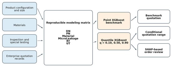
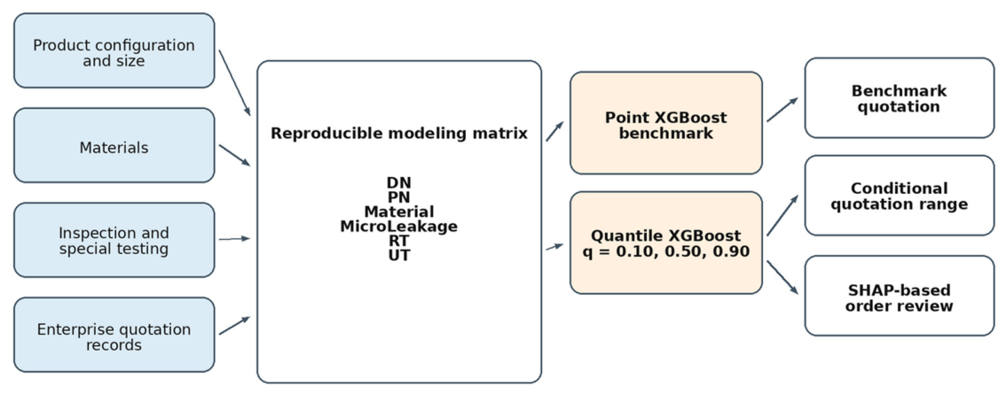
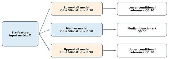
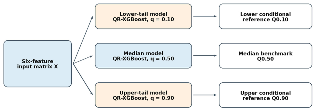
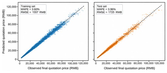
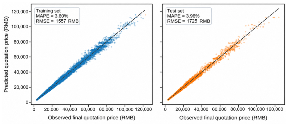
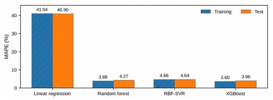
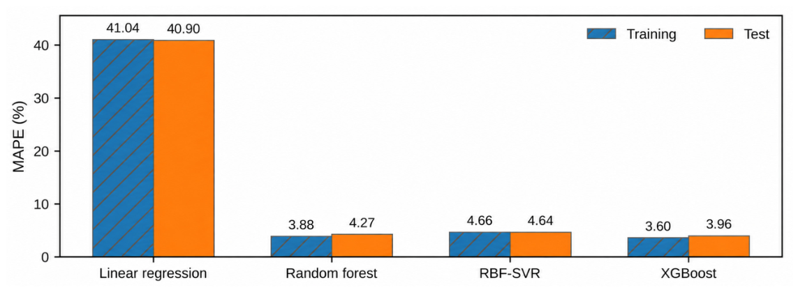
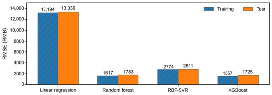
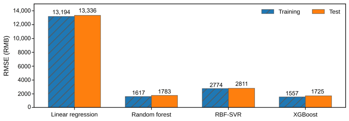
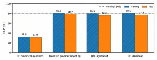
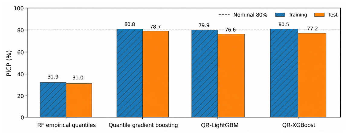
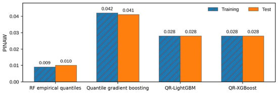
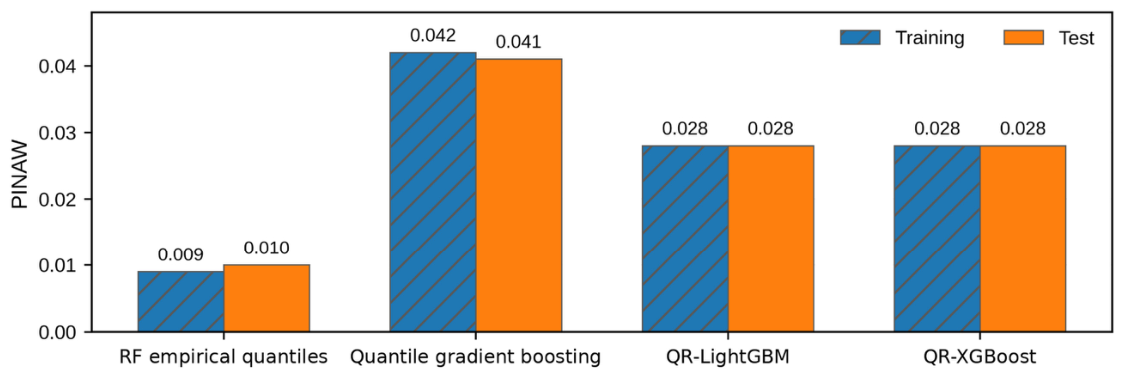
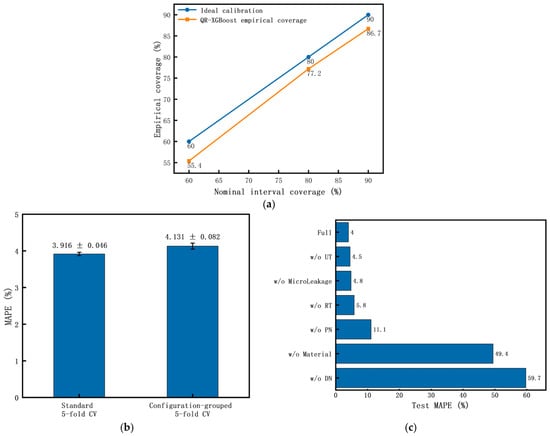
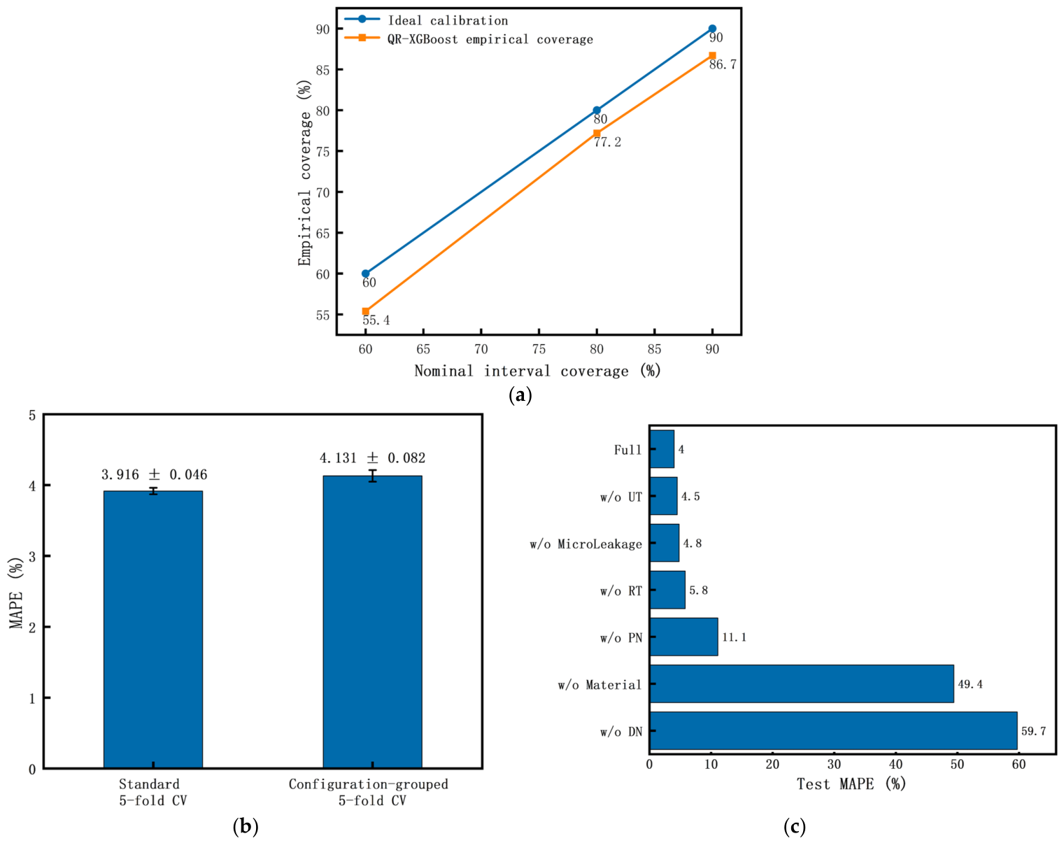
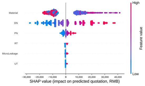
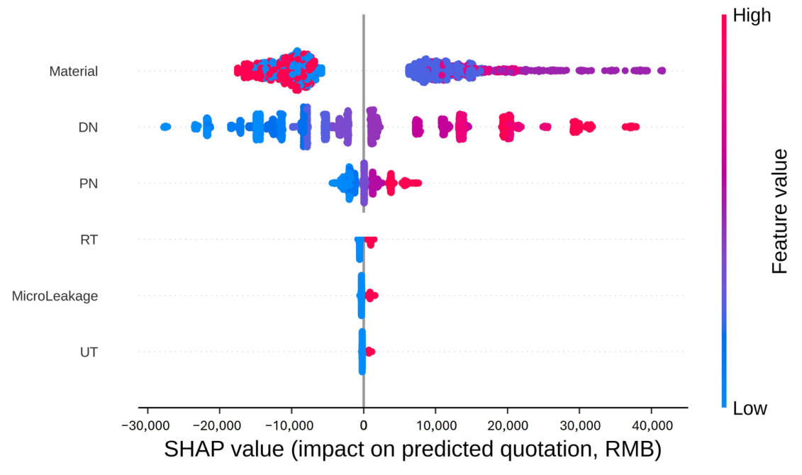
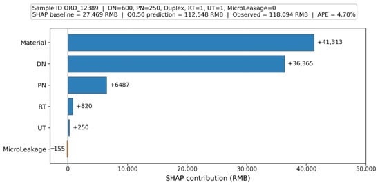
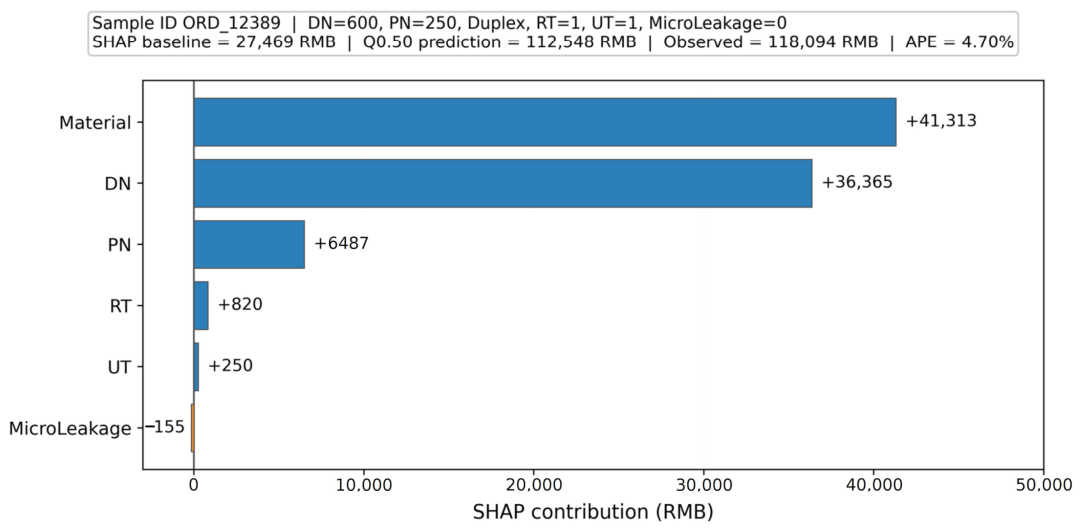

Disclaimer/Publisher’s Note: The statements, opinions and data contained in all publications are solely those of the individual author(s) and contributor(s) and not of MDPI and/or the editor(s). MDPI and/or the editor(s) disclaim responsibility for any injury to people or property resulting from any ideas, methods, instructions or products referred to in the content. |
© 2026 by the authors. Licensee MDPI, Basel, Switzerland. This article is an open access article distributed under the terms and conditions of the Creative Commons Attribution (CC BY) license.