Drone-Based Instant Delivery Hub-and-Spoke Network Optimization

Abstract

Drone-based transportation is emerging as a novel mode in city logistics, featuring first-mile pickup and last-mile instant delivery using drones and truck transshipment. A fundamental challenge involves coordinating merchants, drones, transshipment hubs, trucks, and consumer communities through the hub-and-spoke network (HSN). This study formulated the optimization problem for HSN to minimize logistics costs and loss of orders constrained by service time limits. The ε-constraint model, two evolutionary algorithms based on Non-dominated Sorting Genetic Algorithm II (NSGA-II) using permutation (EAp) and rand key-based (EAr) encoding/decoding schemes were devised to solve the bi-objective mathematical program. Three groups of twelve experiments were conducted using ideal datasets and datasets generated from Shenzhen city to validate the models and algorithms. Relaxing the logistics objective by 10% and subsequently minimizing the loss of orders can significantly reduce average unmet orders by 24.61%; when spokes were beyond 20, the ε-constraint model failed to achieve solutions within an acceptable time. While EAp and EAr demonstrated competence, EAr proved to be more competitive in computation time, hypervolume, spacing metric, and the number of non-dominated solutions on the Pareto fronts. Key parameters influencing the HSN solutions include drone and truck speeds, acceptable delivery times, and the processing and waiting time at hubs.

1. Introduction

Applying drones to urban logistics, particularly in the domain of instant delivery, has emerged as a technological trend, drawing extensive global attention and discourse [1]. Various countries and companies have made significant strides in advancing drone technology and its applications. China continues to develop drone technologies, particularly achieving noteworthy milestones in urban logistics and instant delivery [2]. Companies like Meituan.com, JD.com, and SF Express (sf-express.com) have undertaken substantial efforts in pilot projects for drone-based instant deliveries [3]. Amazon and Google have invested in developing instant-delivery drone technology [4]. European nations actively apply drone technologies in city logistics; e.g., France and the UK are conducting numerous pilot projects [5]. Singapore is a global logistics and technology hub dedicated to advancing drone technologies in city logistics [6].

Large-scale applications of drones in city logistics meet challenges. First, nations must establish pertinent regulations and policies to ensure safe and compliant drone operations within city areas [7]. Second, drone technologies must be mature enough to operate safely and reliably in urban environments while handling complex meteorological and environmental conditions [8]. Implementing an effective air traffic management system for drones is crucial to coordinate and prevent collisions [9]. Given that using drones raises privacy and security concerns, it is essential to take appropriate measures to safeguard personal information and urban infrastructure. Public acceptance also requires extensive societal outreach and education [10]. Constraints and challenges encountered in the application of drones include air traffic congestion, the impact of weather conditions on flights, issues with energy and endurance capabilities, technological barriers, and high costs [10]. With ongoing technical development and the refinement of solutions, the prospects for applying drones to city logistics remain extensive. The benefits of enhancing logistics efficiency, reducing delivery times, and cutting costs will drive the widespread adoption of drones in city logistics. As pertinent regulations are implemented and technology advances [7], the market potential will continue to unfold.

Drone-based logistics harnesses drone technology for urban cargo transportation services, focusing on the swift and immediate delivery of courier services, especially suitable for small packages or urgent items requiring prompt transportation [11]. In contrast to traditional city logistics systems, drone-based instant delivery exhibits distinctive characteristics. Drones can efficiently navigate cities, circumvent traffic congestion, and select the most direct delivery routes, significantly enhancing distribution speed and efficiency [12]. Using drones concurrently reduces labor costs, minimizes energy consumption, and improves overall operational efficiency. Additionally, drone deployment contributes to environmental conservation by mitigating traffic emissions and fostering eco-friendly and sustainable urban development [13]. Lastly, the adaptability of drones enables coverage in a broader range of urban areas, especially within complex urban terrains. Although the drone battery technology is advanced, its flying duration is limited, while mountainous fields and extreme climates may require additional energy consumption.

Drone-based instant delivery addresses a series of decision-making and optimization challenges, including routing drones to minimize time and energy consumption, effectively allocating tasks to drones to maximize overall delivery efficiency, and optimizing the urban storage network to align with the requirements of drone logistics. Addressing these challenges requires applying drone control and navigation technologies, optimization algorithms, theories, methods, and technologies associated with artificial intelligence and big data. Achieving greater efficiency in drone-based instant delivery may require adjustments, optimizations, or reconstructions of existing city logistics networks. For example, constructing infrastructure such as takeoff, landing facilities, and charging stations compatible with drone logistics is necessary [14]. Refactoring the city logistics network to accommodate drone-based instant deliveries is essential. Regulations and policies must also be established to ensure lawful and compliant drone operations.

This study considers the logistics network design and optimization with distinct drone characteristics in urban catering and takeaways orders and delivery: the drones undertake the first-mile pickup and last-mile delivery [15]; the trucks undertake the transshipment; the drones and trucks hand the packages at hubs; the drones conduct pickup and deliver packages from and to specialized intelligent cabinets nearby merchants and consumer communities. Considering these features, we extend the baseline hub-and-spoke network (HSN) model to build a bi-objective program for drone-based instant delivery to minimize logistics costs and loss of orders. The drone and truck speeds affect the transportation time between spokes and hubs and among the hubs. The consumers will raise orders within the accept order engagement time range, e.g., one hour. Thus, the HSN only fulfills such short-time orders, and the network is not fully connected to different general-purpose HSNs. To solve the bi-objective program, we devised an ε-constraint model and then developed two evolutionary algorithms based on Non-dominated Sorting Genetic Algorithm II (NSGA-II) using permutation (EAp) and rand keys (EAr) as encoding/decoding schemes. Using an ideal dataset and the datasets generated in the context of the Shenzhen City case, the devised models and algorithms were compared; the hyperparameters of the evolutionary algorithms were studied; the sensitivities of key parameters were investigated; and some managerial and operations strategies were discussed numerically.

This study contributes to three streams of the literature on drone-based logistics, first- and last-mile logistics, and hub-and-spoke network optimization. First, drone-based logistics mainly focus on routing and coordinating the drones and other devices, e.g., trucks. This study investigates a novel mode featuring drone-based first-mile pickup, last-mile delivery, and truck-based transshipment. Second, most studies are concerned with last-mile distribution by drones, while this study simultaneously formulated first- and last-mile drone operations. Third, consolidation and distribution hubs in logistics networks are generally fully connected. In contrast, this study considered a practical constraint: the order time range that limits the order engagement time upper bounds. Therefore, bi-objective HSN models and algorithms must be developed to optimize the logistics cost and loss of orders.

The rest of the study is organized into six sections. Section 2 reviews the related studies on instant delivery, HSN optimization, and drone-based facility location problems. In Section 3, the problem is described. Section 4 proposes a bi-objective mathematical program by extending a baseline HSN model. Section 5 develops three solution methods based on ε-constraint, NSGA-II, and evolutionary algorithm. In Section 6, three groups and twelve experiments are conducted. Finally, we conclude the study in Section 7.

2. Related Studies

2.1. Instant Delivery

Instant delivery aims to significantly enhance the efficiency of cargo transportation and promptly respond to consumer demands by applying advanced technologies. It integrates the Internet of Things (IoT), artificial intelligence and machine learning (ML), automation and robotics, and big data analytics. It enables the real-time monitoring of the location and status of packages, demand forecasting, routing optimization, and the utilization of autonomous vehicles or robots for delivery tasks. Chinese e-commerce giants such as Alibaba and JD.com have conducted trials of autonomous delivery vehicles [3], and Amazon offers the Prime Now service for two-hour delivery while exploring the possibilities of drone delivery [4]. In instant delivery, drones are considered a robust solution for addressing the last-mile delivery challenge due to their rapidness and flexibility. Drone applications extend beyond last-mile delivery to support emergency supplies transportation and delivery to remote areas.

Instant delivery is limited by the short-order engagement time ranges, e.g., one hour, so advanced technologies and decision-making methods are essential for saving time and speeding the delivery processes. Table 1 lists studies on the operations research of instant delivery, which differs from general delivery in the order engagement time limits [16]. Most studies reviewed apply UAVs (Unmanned Aerial Vehicles) or drones to cooperate with logistics vehicles. The column “TD” (truck and drone) summarizes the transportation devices used. Three studies coordinate trucks and drones for efficient instant delivery. Although even complicated instant delivery problems can be formulated or transferred into mixed-integer linear programs (MILPs), they are challenging to solve by exact algorithms within acceptable times. Various heuristics can be applied to solve the problems. As shown at the end of Table 1, this study investigates the solution of using trucks and drones simultaneously and devises bi-objective MILPs that are solved by algorithms based on $\epsilon$-constraint and NSGA-II.

Table 1. Studies on instant delivery.

Study	Problem Features	TD	Model	Algorithm
[16]	Heterogeneous instant delivery order scheduling and routing problems.	T	MILP	CG
[17]	Instant delivery by vehicles and drones.	TD	MILP	ACO
[18]	An auction-based trading platform to enable procurement for instant delivery.	T	Game	ML
[19]	A facility location and demand allocation problem for drone-based instant delivery.	TD	-	HA
[20]	Online instant delivery with dynamic orders.	T	MILP	GA
[21]	Time-dependent instant delivery considering cost, customer satisfaction, and traffic.	T	MILP	GA, VNS
[22]	A VRP in an instant delivery peak period.	T	MILP	ACO
This study	An HSN coordinating trucks for transshipments among hubs and drones for first-mile pickup and last-mile distribution.	TD	MILP, MO	NSGA-II, GA

Note: ACO = artificial colony algorithm; BG = Benders decomposition; CG = column generation; GA = genetic algorithm; Game = game theory model; HA = heuristic algorithm; MILP = mixed-integer linear program; ML = machine learning; MO = multi-objective optimization; VNS = variable neighborhood search; TD = truck (T) or/and drone (D).

2.2. Hub-and-Spoke Network Optimization

The HSN is a classic model for designing logistics and transportation systems. The network features a set of hubs connecting peripheral spokes, which are interconnected to utilize the economy of scale of logistics. HSN is widely applied in the logistics industry, especially in building efficient supply chain systems for retail and e-commerce [23]. The aviation industry also adopts this concept by connecting different destinations through hub airports to enhance flight operational efficiency [24]. The design of public transportation routes can similarly draw inspiration from the HSN concept to achieve efficient connections [12]. The theoretical and technical challenges in designing and optimizing HSNs include addressing distinct features, developing faster solutions, and considering uncertain and dynamic demands, traffic, and network structures.

Many studies have investigated HSN optimization, as presented in Table 2. The HSNs have been applied in waterways [25], maritime [26], roads [27], railroad [28], and aviation transportation and logistics systems. Generally, the hubs are not fully connected to waterways and maritime transportation systems. In this study, the hub connections are constrained by order engagement time ranges. In the column “PF” (partial or complete connections among hubs), some studies consider the partial connections practically [25,28,29,30]. The HSN involves logistics costs, efficiency, and emissions, so it should be formulated as a multi-objective model. Although it can be formulated as MILPs, due to its complexities, various math-heuristics and metaheuristics have been developed in the literature. As elucidated in the last row in Table 2, we considered minimizing the logistics cost and order loss simultaneously in a bi-objective model, which is solved by $\epsilon$-constraint and NSGA-II.

Table 2. Pioneering studies on hub-and-spoke network optimization.

Study	Problem Features	PF	Model	Algorithm
[31]	A hierarchical urban and rural logistics network with hub capacity and demand uncertainty.	F	MILP	B&C
[32]	Reconfiguring the merged HSNs considering vehicle emissions, on-time delivery, and operating costs.	F	MO, MINLP	SOCP
[28]	An HSN network for railroad freight with links to concentrated freight flows.	P	MILP	HA
[30]	Service networks based on round-trips.	P	MILP	VNS, ML
[25]	Inland container shipping HSN networks, determining hubs, feeder port allocation, and fleet deployment.	P	MILP	BD
[33]	HSN network design considering congested hubs and links.	F	Queue	NSGA-II, ILS
[34]	Hub location considering links with incentive-dependent capacities, affecting the hub selections and flow assignment.	P	Convex	Approx
[24]	A cross-docking HSN with electric truck fleets, mobile charging stations, and capacity constraints.	F	Graph	GA
This study	Drones undertake transportation between spokes and hubs, while trucks undertake transshipment among hubs. Instant delivery time ranges constrain the connections among hubs.	P	MILP, MO	GA, NSGA-II

Note: Approx = outer-approximation algorithm; B&C = branch-and-cut algorithm; BD = Benders decomposition; ILS = Iterated Local Search; MINLP = mixed-integer nonlinear program; SOCP = second-order cone program.

2.3. Drone-Based Facility Location Problems

The application of drone technology to logistics is gradually becoming widespread, bringing forth new features and challenges in facility location problems. These features consider the rational spatial utilization and safety requirements of drone takeoff and landing facilities, charging stations, and maintenance to ensure sustained and stable drone operations. Various new technologies and methods with drone-based logistics systems are applied to facility locations. Virtual reality and simulation technologies are used to simulate location selection scenarios virtually, evaluating the operational effectiveness of drones in different locations [35]. Data analytics and predictive technologies help assess the demands and potential traffic at various locations, while autonomous navigation and environmental perception technologies ensure safe and effective drone flights in urban environments [12]. However, limitations include short endurance [36], susceptibility to weather conditions, regulation challenges [7], and privacy protection.

Table 3 reviews pioneering studies on drone-based routing and location optimization in three aspects: problem features, model, and algorithm. Three classification criteria are further developed to study the problem features: FL (first-mile pickup or last-mile delivery), RN (routing or network optimization), and FD (fixed or dynamic drone launching and returning locations). In all reviewed studies, drones undertake the last-mile delivery tasks. Most studies concern the truck/vehicle and drone routing problem, and some consider the locations of drone launching and returning, while these locations depend on the truck routes. As for models, although some studies formulate the problems as MILPs, they also analyze the problems and devise models by scenario-based sensitivities. The above studies correlate well with methodology, while the large-scale drone application in urban distribution may challenge management, the environment, and safety.

Table 3. Related studies on drone-based routing and location optimization.

Study	Problem Features	FL	RN	FD	Model	Algorithm
[37]	Minimize the makespan in TDRP with non-customer stops.	L	R	D	MILP	SA, VNS
[29]	TDRP with uncertain demands and drone capacity.	L	R	F	MILP	SAA, GA
[38]	TDRP with synchronization on arcs.	L	R	D	MINLP	ALNS
[39]	Drone launch/retrieval with a moving truck.	L	N	F	SP	GA, HA
[12]	Drone routing constrained by traversal time and limited batteries.	L	R	D	SP	SAA
[35]	Locate drone takeoff platforms.	L	R	F	Graph	BD
[11]	Robust drone TSP with uncertain travel time.	L	R	D	RO	B&PC, HA
[40]	Optimize contactless delivery risk and makespan.	L	FN	F	SP	BD
[41]	Minimize customer waiting times in multi-trip one-truck and multi-drone routing.	L	FN	F	MO	NSGA-II, TS
This study	Minimize customer waiting times in multi-trip one-truck and multi-drone delivery.	FL	RN	FD	Model	Algorithm

Note: B&PC = branch-and price-and-cut algorithm; FD = fixed and/or dynamic drone launching and returning locations; FL = first-mile pickup and/or last-mile delivery; MINLP = mixed-integer non-linear program; RO = robust optimization; SA = simulated annealing; SAA = sample average approximation; SP = stochastic program; TS = tabu search algorithm.

Due to the complexities of the truck–drone routing problem (TDRP) and location optimization models, exact algorithms (e.g., B&PC and BD) and various heuristic algorithms (e.g., ALNS, GA, and TS) contribute to obtaining optima or approximate solutions. As indicated in the last row of Table 3, this study was activated by drone-based urban instant delivery and aimed to optimize the HSN coordinating drones and trucks. In particular, the drones undertake the first-mile pickup from merchants to hubs and last-mile delivery from hubs to consumers, while the trucks serve the transshipment among hubs. Therefore, the drone launching and returning hubs incur a strategic decision. We formulated the problem as a bi-objective MILP, which was solved using $\epsilon$-constraints and NSGA-II.

3. Problem Statement

As a Chinese technology retail company, Meituan (www.meituan.com, accessed on 4 June 2024) has launched an advanced drone-based instant delivery service in Shenzhen, primarily applied in scenarios such as tourist attractions, parks, community office buildings, and residential areas, providing consumers with marvelous, efficient, safe, and convenient takeaway ordering experiences. Shenzhen City is critical in developing drone technologies and applications in China and worldwide. The local governments set up positive technology, economy, and regulation environments to promote drone experiments and marketable applications. Meituan’s drone-based instant delivery service began active exploration in 2017 and successfully initiated the first domestic industrial park drone-based instant delivery route in China in Shenzhen in 2021. By 2023, the service operated 17 routes in cities, including Shenzhen and Shanghai, completing over 184,000 orders and delivering efficient consumer services [42].

As a notable feature, drone-based instant delivery utilizes cutting-edge technologies, including navigation, obstacle avoidance, three-dimensional visual mapping, and routing control intelligent devices and technologies. Advanced technologies enable drones to use autonomous flight and airborne traffic management, enhancing flight safety and stability. Drone-based instant delivery effectively mitigates road congestion and environmental pollution [43,44], aligning with green and low-carbon development targets.

Despite the significant achievements, drone-based instant delivery still faces challenges and difficulties, including issues related to the city logistics system with drones, operating costs, technologies, regulations, and consumer behaviors. Addressing these challenges requires further in-depth exploration and refinement to adapt to market demands and enhance the quality and sustainability of the service.

To improve logistics operations management performances, we investigated the solutions based on HSN for cooperating with drone-based first-mile pickup and last-mile delivery.

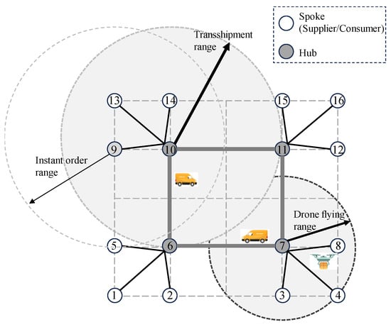
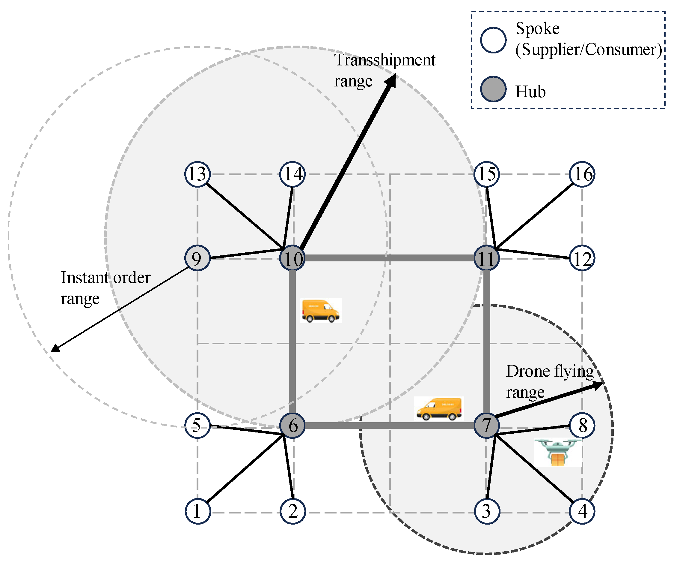
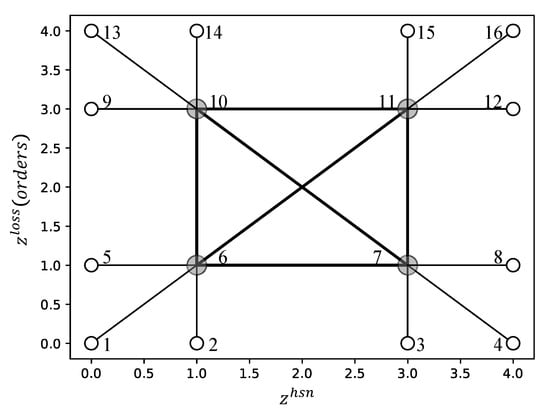
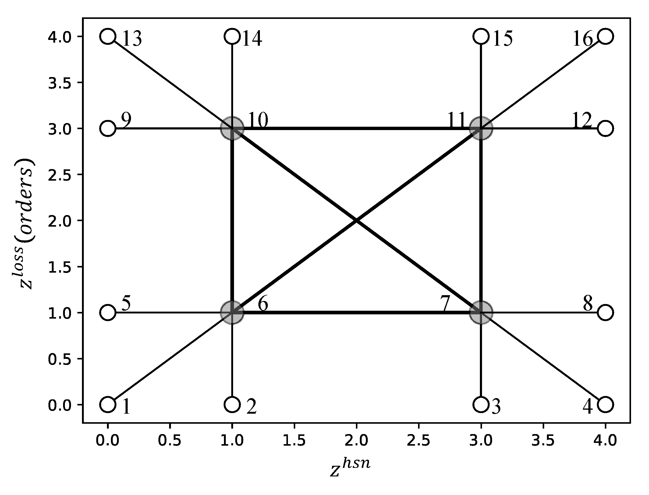
Typically, an HSN consists of a set of spokes ($S$) and a minor set of hubs ($H$). The logistics flow among two given spokes, $i,j$, is denoted by $W_{ij}$, and the distance is $C_{ij}$. Indeed, the terrain will impact the distance between any two points and even the climate. Thus, we can further compute $C_{ij}$ considering real-world 3D trajectories, even considering constraints by airspace regulations and discretization. The HSN operator should select a set of spokes to be fully connected hubs to achieve the economy of scale of logistics operations among the hubs. Thus, the unit consolidation cost is defined from spokes to hubs, the transshipment cost among hubs, and the distribution cost from hubs to spokes as $P^C,P^T,P^D$, generally, $P^C>P^D>P^T$. Without a loss of generality and for simplification purposes, we created an ideal example, as presented in Figure 1, to explain the related concepts and entities. In Figure 1, the HSN has 16 spokes and four hubs. Here, each spoke is assigned to only one hub entitled single-allocation HSN.

Figure 1. A demonstrative diagram of drone-based instant delivery.

As illustrated in Figure 1, drones pick up packages from spokes and send them to hubs. Then, the packages are gathered and transshipped among the hubs by trucks. Finally, some drones load the packages from the hubs and deliver them to the target spokes. In the above processes, the consumers will only raise orders within an instant order engagement time range (denoted by $T^{order}$), generally one hour in the urban catering and takeaway delivery scenarios. The drones can only take tasks within flying duration limits. The trucks and drones can only travel at given speeds (denoted by $S^{truck},S^{drone}$). Under the above premises, the HSN hubs are not always connected entirely under the constraint of $T^{order}$. Thus, the hubs incur transshipment ranges. Considering this feature, the HSN should be sparse because the long connections among hubs will be eliminated.

4. Formulation

4.1. Baseline Hub-and-Spoke Optimization Model

The parameters and decision variables are defined in the baseline HSN optimization model. $S$ is a set of spokes, $S=\left\{\mathrm{1,2},3,\dots \right\}$. $C_{ij}$ is the distance between two spokes, $i,j\in S,C_{ii}=0$. $P^C,P^D,P^T$ are the costs of transporting a unit of packages for a unit of distance from spokes to hubs, among hubs, and from hubs to spokes. The cargo flow from a spoke $i\in S$ to another $j\in S$ is $W_{ij}$. $O_i,D_i$ represent the in- and out-flows of the spoke $i\in S$, namely, $O_i={\sum }_j{W}_{ij},D_i={\sum }_j{W}_{ji}$.

Two decision variables are defined: $x_{ik}$ and $y_{ikh}$. When $x_{ik}=1$, the spoke $i\in S$ is assigned to the hub $k\in S$ and $x_{kk}=1$; then, $k$ is a hub. $y_{ikh}$ is the cargo flow from the spoke $i$ through the hub $k$ and then the hub $h$, $i,k,h\in S$. The hub set is denoted by $H$, $H\subseteq S$. In literature, the cost of $i\in S$ to be a hub is denoted by $F_i$. Hub investment is a strategic problem. We introduced the number of hubs to be chosen, $\overline{H}$, namely, $\overline{H}=\left|H\right|$.

The above notations are summarized as follows.

Sets
$S,H,\overline{H}$	$S$  is a set of nodes, namely, spokes and potential hubs; H is a set of hubs, and $\overline{H}$ is the number of hubs.
Data
$C_{ij}$	Distance from the node $i\in S$ to $j\in S$, $C_{ii}$  = 0 for all $i\in S$; assume that the triangle inequality is satisfied,$C_{ij}\le C_{ik}+C_{kj},i,j,k\in S.$
$P^C,P^D,P^T$	The consolidation (from spokes to hubs), transshipment (among hubs), and distribution (from hubs to spokes) cost discounts.
$W_{ij}$	Cargo flow from the node $i\in S$ to $j\in S$
$O_i={\sum }_j{W}_{ij}$	Cargo flow originated from the node $i\in S$
$D_i={\sum }_j{W}_{ji}$	Cargo flow destinated to the node $i\in S$
$\overline{H}$	Number of hubs.
Variables
$x_{ik}\in \left\{\mathrm{0,1}\right\}$	$x_{ik}=1$  if the spoke i is assigned to the hub k; otherwise, 0. $x_{kk}=1$ represents that k is chosen as a hub.
$y_{ikh}\ge 0$	The flow originated from the spoke $i\in S$, through the hubs k and h sequentially to the target spoke $(i,k,h\in S).$

The HSN optimization problem can be formulated as a cost minimization model [M1], where the total cost ($z^{hsn}$) consists of consolidation ($z^C$), transshipment ($z^T$), and distribution ($z^D$) costs, as denoted by (1), (2), (3), and (4).

$$\left[\mathrm{M}1\right]\min z^{hsn}=z^C+z^T+z^D,$$

(1)

where

$$z^C={\sum }_{ik}{P}^C{C}_{ik}{O}_i{x}_{ik},$$

(2)

$$z^T={\sum }_{ikh}{P}^T{C}_{kh}{y}_{ikh},$$

(3)

$$z^D={\sum }_{ik}{P}^D{C}_{ki}{D}_i{x}_{ik},$$

(4)

subject to

$${\displaystyle \sum _k}{x}_{ik}=1,\forall i$$

(5)

$$x_{ik}\le x_{kk},\forall i,k$$

(6)

$$\sum _k{x}_{kk}=H$$

(7)

$$\sum _h{y}_{ikh}-\sum _h{y}_{ihk}=O_i{x}_{ik}-\sum _j{W}_{ij}{x}_{jk},\forall i,k$$

(8)

$$\sum _{h\ne k}{y}_{ikh}\le O_i{x}_{ik},\forall i,k$$

(9)

$$x_{ik}\in \left\{\mathrm{0,1}\right\},\forall i,k$$

(10)

$$y_{ikh}\ge 0,\forall i,k,h$$

(11)

The constraint (5) constrains that a spoke can be assigned to one and only one hub. In (6), a spoke can accept flows from spokes only when it is chosen as a hub. The number of hubs is given in (7). The flow originating from a spoke is determined by (8) and (9). The variable domains are given in (10) and (11).

4.2. Extended Bi-Objective Optimization Models

Unlike the general HSN solutions defined in [M1], the investigated instant logistics solution uses drones for first-mile pickup and last-mile delivery [45]. The consumers raise takeaways orders under the consideration of the acceptable order engagement time range ($T^{order}$) between their locations and the merchants. Therefore, some orders may be unacceptable because the total logistics time exceeds $T^{order}$.

For a given pair of spokes $i,j$, the total logistics time accomplishing the pickup, transshipment, and delivery is denoted by ${\tilde{t}}_{ij}^{order}$, which consists of five parts: drone-based pickup time, processing and waiting time at the consolidation hub, truck transshipment time from the consolidation hub to the distribution hub, the processing and waiting time at the distribution hub, and the drone-based delivery time. To simplify the formulation, we use $A\left(i\right)$ to represent the hub assigned to the spoke $i$. If ${\tilde{t}}_{ij}^{order}>T^{order}$, the order is likely to be lost because the consumer may not accept a later delivery. Indeed, the consumer raises the order to consider (13), and the takeaway ordering platforms must consider such criteria.

$${\tilde{t}}_{ij}^{order}=\frac{C_{iA\left(i\right)}}{S^{drone}}+T^{tr}+\frac{C_{A\left(i\right)A\left(j\right)}}{S^{truck}}+T^{tr}+\frac{C_{A\left(j\right)j}}{S^{drone}}$$

(12)

$$\frac{C_{ij}}{S^{truck}}\le T^{order}$$

(13)

The drone-based logistics solution changes the components of time in the order engagement. Therefore, the decision-makers must improve the logistics network and operations to minimize the loss of orders.

To formulate the minimization of the loss of orders, we introduced additional variables besides ${\tilde{t}}_{ij}^{order}$. First, $t_{ijkh}^{tr}$ represents the transshipment time by a truck from the hub $k$ to the hub $h$ in the engagement of the order from the spoke $i$ to the spoke $j$. $t_{ijkh}^{tr}$ can be determined by (14) when $k$ and $h$ are hubs of $i$ and $j$. Second, $t_{ij}^{tr}$ is the transshipment time by a truck, which is computed based on $t_{ijkh}^{tr}$, as calculated in (15). Third, a binary variable $z_{ij}$ is defined, indicating whether the order $\left(i,j\right)$ will be lost or not, as denoted in (16). Finally, the loss of orders can be expressed in (17).

$$t_{ijkh}^{tr}\ge \frac{C_{kh}}{S^{truck}}\cdot \left(x_{ik}+x_{hj}-1\right)$$

(14)

$$t_{ij}^{tr}=\sum _{kh}{t}_{ijkh}^{tr}$$

(15)

$$z_{ij}\cdot M\ge {\tilde{t}}_{ij}^{order}-T^{order},\forall i,j$$

(16)

$$f^{loss}=\sum _{ij}{z}_{ij}{W}_{ij}$$

(17)

A revised model was then formulated as [M2].

$$\left[\mathrm{M}2\right]\min \left(z^{hsn},z^{loss}\right)$$

Subject to

Constraints ((1)–(9), (14)–(17)).

$$x_{ik}\in \left\{\mathrm{0,1}\right\},y_{ikh}\ge 0,z_{ij}\in \left\{\mathrm{0,1}\right\},t_{ijkh}^{tr}\ge 0,t_{ij}^{tr}\ge 0,\forall i,k,h$$

The known data of the model can be represented by a vector ($\mathbf{I}$), and the variables can be represented by $\mathbf{X}$, as denoted by (18) and (19).

$$\mathbf{I}=\left[S,W,C,P^C,P^D,P^T,D,O,S^{drone},S^{truck},T^{tr},T^{order}\right]$$

(18)

$$\mathbf{X}=\left[x_{ik},y_{ikh},z_{ij},z^{hsn},z^{sum},z^C,z^T,z^D,t_{ij}^{tr},t_{ijkh}^{tr}|\forall i,j,k,h\right]$$

(19)

5. Solution Algorithm

5.1. Solving Bi-Objective Models by $\epsilon$-Constraints

As formulated in Section 4.2, [M2] is a bi-objective model, which can be solved based on $\epsilon$-constraints

First, we can optimize [M2] by minimizing the single objective $z^{hsn}$, which can be denoted by [M2a], as defined in (20). We can use $f^{\left[\mathrm{M}2\mathrm{a}\right]}\left(\cdot \right)$ to represent the solving process (21), where $z^{hsn\ast },X^{\ast }$ are the solution values of the variables.

$$\left[\mathrm{M}2a\right]\min \left\{z^{hsn}|\left(\left(1\right)-\left(17\right)\right)\right\}$$

(20)

$$z^{hsn\ast }\leftarrow X^{\ast }\leftarrow f^{\left[\mathrm{M}2\mathrm{a}\right]}\left(\mathrm{I}\right)$$

(21)

Second, we can formulate a new model to consider the relaxation of $z^{hsn}$ by considering a new constraint with a relaxation coefficient $\epsilon \ge 0$, as denoted in (22).

$$\left[\mathrm{M}2\left(\epsilon \right)\right]\min \left\{z^{loss}|\left(\left(1\right)-\left(17\right)\right);z^{hsn}\le \left(1+\epsilon \right)z^{hsn\ast }\right\}$$

(22)

Third, by iterating the acceptable values of $\epsilon$, we can obtain the pairs of $\left(z^{hsn},z^{loss}\right)$ to construct Pareto fronts between the two objectives, $z^{hsn}$ and $z^{loss}$.

The $\epsilon$-constraint method, as formulated in (22), converts the bi-objective model [M2] into a computable model. For each value of $\epsilon$, [M2] is solved to obtain the two objectives through the constraint ($z^{hsn}\le \left(1+\epsilon \right)z^{hsn\ast }$) and objective ($z^{loss}$) in (22). When [M2] can be solved mathematically, it can provide a tight Pareto front. However, solving [M2] is time-consuming and does not apply to practical instances with more than 20 nodes (see Section 6.4.4).

5.2. Evaluating Solutions with Determined Hubs

Algorithm 1 evaluates solutions with given hubs, assigns hubs to spokes, and calculates the logistics cost $z^{hsn}$ and the order loss $z^{loss}$.

Algorithm 1. Evaluate an HSN solution determined by given hubs (eval)
Inputs	$\mathrm{Data}: \mathbf{I}.$
	A set of hubs,$hubs$.
Outputs	Logistics cost and loss of orders,$z^{hsn},z^{loss}$.
Steps
Step 1	Assign spokes to hubs
	$A\left(s\right)=\arg \underset{k\in \mathit{hubs}}{\min }distance\left(s,k\right),\forall s\in S$.
Step 2	Calculate logistics cost $z^{hsn}$
	$z^C={\sum }_{i\in S}{P}^C{O}_i{C}_{iA\left(i\right)}$.
	$z^D={\sum }_{i\in S}{P}^D{D}_i{C}_{A\left(i\right)i}$.
	$z^T={\sum }_{i,j\in S}{P}^T{W}_{ij}{C}_{A\left(i\right)A\left(j\right)}$.
	$z^{hsn}=z^C+z^T+z^D$.
Step 3	Calculate loss of orders $z^{loss}$
	$t_{ij}^{order}=\frac{C_{iA\left(i\right)}}{S^{drone}}+T^{tr}+\frac{C_{A\left(i\right)A\left(j\right)}}{S^{truck}}+T^{tr}+\frac{C_{A\left(j\right)j}}{S^{drone}},\forall i,j,W_{ij}>0$.
	$z^{loss}={\sum }_{ij;t_{ij}^{order}>T^{order}}{W}_{ij}$.
Step 4	Return $z^{hsn},z^{loss}$

Algorithm 1 can be denoted by $f^{eval}$ as follows:

$$z^{hsn},z^{sum},x^{\ast }\leftarrow f^{eval}\left(\mathbf{I};hubs\right)$$

5.3. Evolutionary Algorithms Based on NSGA-II

5.3.1. Introducing NSGA-II-Based EAs

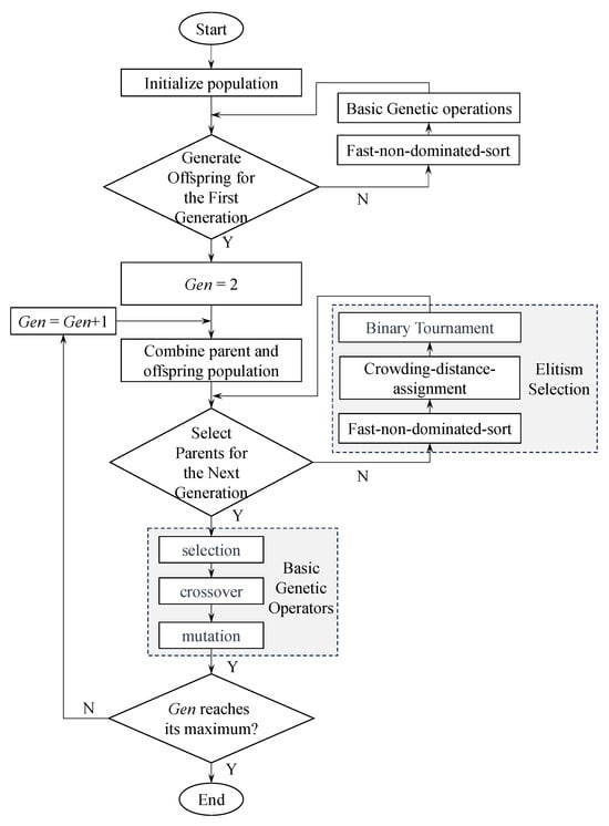
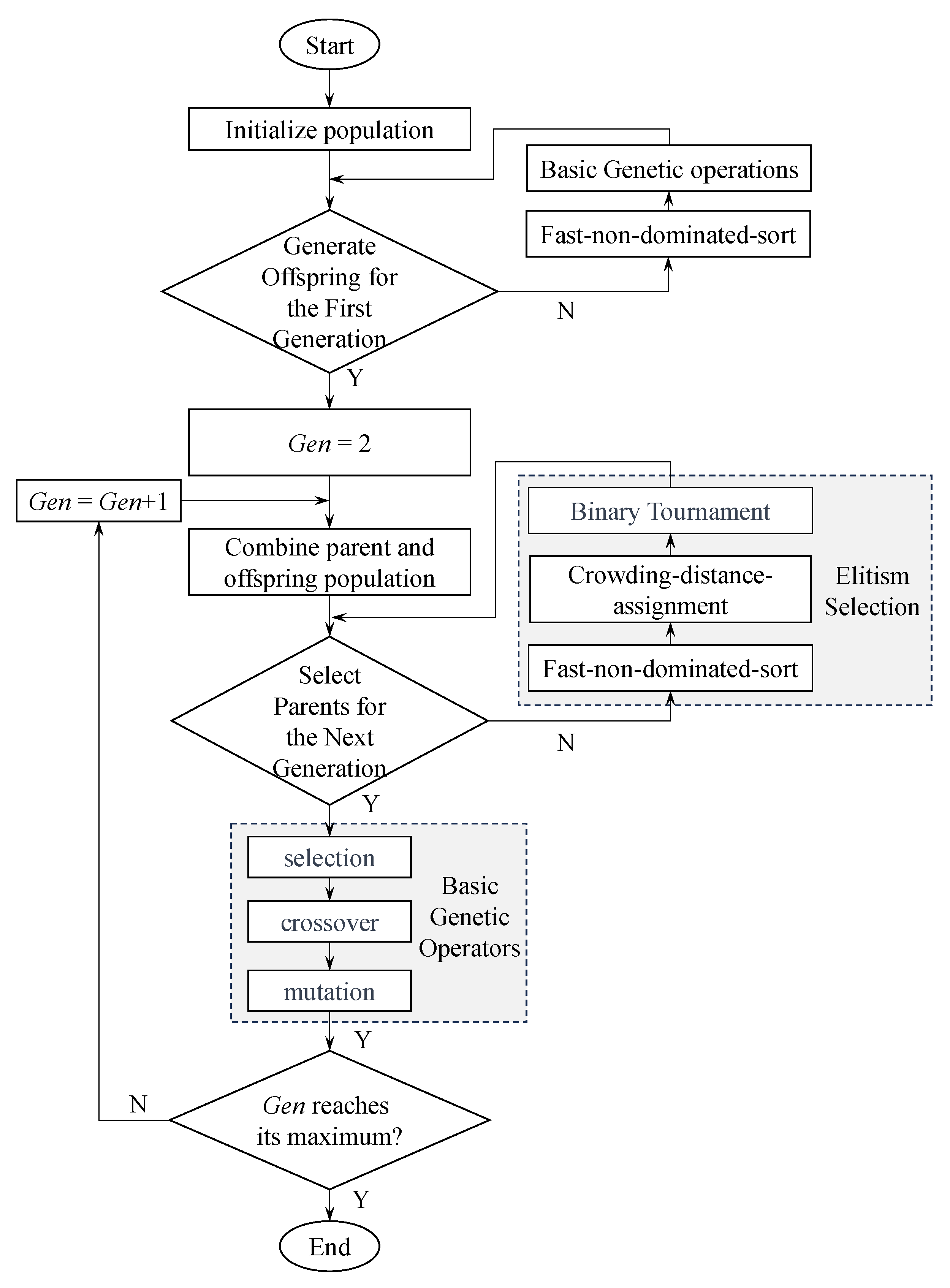
NSGA-II addresses the multi-objective optimization problems (MOP). The algorithm has been proven effective in solving real-world MOPs in various domains, promoting diversity and convergence of Pareto-optimal solutions. Many MOP solution algorithms have been developed, while NSGA-II is widely used in literature and practice and is a typical base of most other MOP algorithms. NSGA-II ranks the population through non-dominated sorting, calculates the crowding distance of individuals in the population to maintain diversity, and obtains an approximate solution when the termination condition is met [46]. The basic flowchart of the NSGA-II algorithm is shown in Figure 2. The algorithm employs a fast, non-dominated sorting method, reducing the algorithm’s computational complexity from $O\left(m{N}^3\right)$ to $O\left(m{N}^2\right)$ ($m$ is the number of objective functions, and $N$ is the population size), significantly decreasing the computation time [47]. The introduced method for calculating crowding distance avoids the issue of manually specifying the sharing radius in fitness-sharing strategies [48]. The elite strategy is adopted, merging parent and offspring individuals for non-dominated sorting, expanding the search space [46]. Individuals with higher priority are selected to generate the next generation of parent populations. Within the same priority level, the binary tournament strategy is employed based on crowding distance to select high-quality individuals in the population [49], which ensures that excellent individuals have a greater chance of being retained.

Figure 2. A diagram of NSGA-II.

5.3.2. An Evolutionary Algorithm Framework Based on NSGA-II

We devised an EA framework (Algorithm 2) based on NSGA-II to obtain Pareto fronts as defined in [M2]. The population size is set to $P^n$, the maximum number of generations is $P^{gen}$, the mutation probability is $p^m$, and the crossover probability is $p^c$. Based on the characteristics of the model, we encoded the decision variables and thus devised decoding schemes correspondingly denoted by $f^{decode}\left(\cdot \right)$, as defined by Algorithms 3 and 4 in Section 5.3.3.

Algorithm 2. An EA based on NSGA-II for HSN optimization (EA)
Inputs	$\mathrm{Data}: I=\left[S,W,C,P^C,P^D,P^T,D_i,O_i,S^{drone},S^{truck},T^{tr},T^{order}\right].$
	Hyperparameters: Population Size $(P^n$); Maximum number of generations $(P^{gen}$); Mutation probability $(P^m$); Crossover probability $(P^c$); Objective function $(f^{decode}\left(\cdot \right)$).
Outputs	Pareto front solutions.
Step 1	Initialization
	Set $Gen=1$
	Generate an initial population $\left({\mathcal{P}}_{gen}\right)$ of $P^n$ individuals randomly in the decision variable space.
	Evaluate the objective values for each individual.
	$\left(z^{hsn},z^{loss}\right)\leftarrow f^{decode}\left(\mathbf{I},pop\right),\forall pop\in PO{P}_{Gen}$.
Step 2	Non-dominated sorting
	Perform non-dominated sorting to divide the population into fronts $\left(F_1,F_2,\cdots ,F_n\right)$.
	Assign a rank to each individual based on its front.
Step 3	Termination
	If the termination criterion (e.g.,$Gen>P^{gen}$) is met, Go to Step 8.
Step 4	Crowding distance assignment
	Calculate the crowding distance for each individual on each front.
	Assign the crowding distance to measure the density of solutions around each individual.
Step 5	Create Offspring Population
	Initialize an empty offspring population.
	${\mathcal{P}}^{os}=\mathrm{\varnothing }$.
	Repeat until the offspring population is filled:
		Perform binary tournament selection based on non-domination and crowding distance to get two individuals $\left(po{p}_1,po{p}_2\right)$ from ${\mathcal{P}}_{gen}$.
		Apply crossover with probability $P^c$ to produce two children. $\left(po{p}_a,po{p}_b\right)\stackrel{crossover}{\leftarrow }\left(po{p}_1,po{p}_2\right)$.
		Apply mutation with probability $P^m$ to each child of $\left(po{p}_a,po{p}_b\right)$. $po{p}_a\stackrel{mutation}{\leftarrow }po{p}_a,po{p}_b\stackrel{mutation}{\leftarrow }po{p}_b$.
		Evaluate the objective values for the children. $\left(z^{hsn},z^{loss}\right)\leftarrow f^{decode}\left(pop\right),\forall pop\in \left\{po{p}_a,po{p}_b\right\}]$.
		Fill the new offspring into ${\mathcal{P}}^{os}$.
		${\mathcal{P}}^{os}\leftarrow {\mathcal{P}}^{os}\cup \left\{po{p}_a,po{p}_b\right\}$.
Step 6	Merge Populations.
	Combine the parent $\left({\mathcal{P}}_{gen}\right)$ and offspring $({\mathcal{P}}^{os}$) populations.
	${\mathcal{P}}^m\leftarrow {\mathcal{P}}_{gen}\cup {\mathcal{P}}^{os}$.
Step 7	Tournament selection
	Perform non-dominated sorting and crowding distance assignment on the combined population.
	Select the top $P^n$ individuals from $2P^n$ individuals in ${\mathcal{P}}^m$ based on non-domination rank and crowding distance.
	$Gen\leftarrow Gen+1$.
	${\mathcal{P}}_{Gen}\stackrel{tournament}{\leftarrow }{\mathcal{P}}^m$.
	Go to Step 2
Step 8	Output
	The final set of non-dominated solutions, $\left(F_1,F_2,\cdots ,F_n\right)$.

Algorithm 2 can be denoted by $f^{\left[\mathrm{E}\mathrm{A}\mathrm{p}\right]}\left(\cdot \right)$ and $f^{\left[\mathrm{E}\mathrm{A}\mathrm{r}\right]}\left(\cdot \right)$, depending on the decoding scheme used, namely, the permutation (EAp) and random key (EAr).

5.3.3. Encoding/Decoding Schemes Based on Permutation and Random Keys

• Permutation-Based Encoding/Decoding Scheme

The permutation-based individual representation encodes the HSN solutions into a vector of spoke indices and chooses the first $\overline{H}$ ones as hubs, and the costs of hubs are evaluated using Algorithm 1. The whole decoding steps are given in Algorithm 3.

Algorithm 3. Permutation-base decoding $(f^p$)
Inputs	The number of hubs,$\overline{H}$; A vector of indexed spokes,$S$; A vector of permutated spokes,$chroms$.
Outputs	Values of the two objectives,$z^{hsn},z^{sum}$.
Steps
Step 1	Slice the first $\overline{H}$ genes in $chroms$ in to $s$. $s=chroms\left[1,\dots ,\overline{H}\right]$.
Step 2	Map each index in s into the spoke as a hub, denoted by $hubs$.
	$hubs=\left\{S\left[i\right]|\forall i\in s\right\}$.
Step 3	Obtain the objective values by Algorithm 1.
	$z^{hsn},z^{loss},x^{\ast }\leftarrow f^{\left[\mathrm{A}1\right]}\left(I;hubs\right)$.
Step 4	Return $z^{hsn},z^{loss}$

Algorithm 3 can be denoted by $f^p\left(\cdot \right)$:

$$z^{hsn},z^{loss}\leftarrow f^p\left(\overline{H},S;chroms\right).$$

Because $\overline{H},S$ are parts of the known data $I$ of the HSN, we can use $f^p\left(chroms\right)$ for simplicity.

2.

Random key-based encoding/decoding scheme

The random key-based encoding scheme uses a vector of $2\overline{H}$ genes with values in $\left[\mathrm{0,1}\right]$. These values are mapped to coordinates in the space determined by the coordinates of all spokes. Then, the spoke closest to each coordinate is set to a hub. Algorithm 4 gives the steps where $X^{-},X^{+},Y^{-},Y^{+}$ are the minimum and maximum of the coordinates of the spokes, calculated as Equation (23).

$$X^{-}=\underset{i\in S}{\min }X\left[i\right]$$

(23)

$$X^{+}=\underset{i\in S}{\max }X\left[i\right]$$

$$Y^{-}=\underset{i\in S}{\min }Y\left[i\right]$$

$$Y^{+}=\underset{i\in S}{\max }Y\left[i\right]$$

Algorithm 4. Random key-based decoding  $(f^r$)
Inputs	The number of hubs,$\overline{H}$; A vector of spokes, and its coordinates,$S,X,Y$; The ranges of spokes’ coordinates,$X^{-},X^{+},Y^{-},Y^{+}$; A vector of random keys,$chroms$.
Outputs	Values of the two objectives,$z^{hsn},z^{sum}$.
Steps
Step 1	Initialize the set of hubs,$hubs=\varnothing$.
Step 2	Get the random keys $(x_i^{rk},y_i^{rk})$ for each potential hub i.
	$x_i^{rk}=chroms\left[i\right],y_i^{rk}=chroms\left[i+\overline{H}\right],\forall i\in \left\{\mathrm{1,2},\cdots ,\overline{H}\right\}$.
Step 3	Map the random keys into coordinates for each hub i.
	$x_i^{co}=X^{-}+x_i^{rk}\left(X^{+}-X^{-}\right),\forall i\in \left\{\mathrm{1,2},\cdots ,\overline{H}\right\}$. $y_i^{co}=Y^{-}+x_i^{rk}\left(Y^{+}-Y^{-}\right),\forall i\in \left\{\mathrm{1,2},\cdots ,\overline{H}\right\}$.
Step 4	For each $i\in \left\{\mathrm{1,2},\cdots ,\overline{H}\right\}$:
	Find the nearest spoke to the coordinates $(x_i^{co},y_i^{co})$ for the hub i.
	$s_i\leftarrow \arg \underset{k\in S}{\min }\left\{distance\left(X\left[k\right],Y\left[k\right],x_i^{co},y_i^{co}\right)|\forall k\in S\backslash hubs\right\}$.
	Update the hub set:$hubs\leftarrow hubs\cup \left\{s_i\right\}$.
Step 5	Obtain the objective values by Algorithm 1.
	$z^{hsn},z^{sum},x^{\ast }\leftarrow f^{\left[\mathrm{A}1\right]}\left(I;hubs\right)$.
Step 6	Return $z^{hsn},z^{sum}$

Algorithm 4 can be denoted by $f^r\left(\cdot \right)$:

$$z^{hsn},z^{loss}\leftarrow f^r\left(\overline{H},S;chroms\right).$$

Because $\overline{H},S$ are parts of the known data $\mathbf{I}$ of the HSN, we can use $f^r\left(chroms\right)$ for simplicity.

The notated function $f^{decode}\left(\cdot \right)$ is introduced to represent the above two algorithms, $f^p$ and $f^r$, namely, $decode\in \left\{p,r\right\}$.

5.3.4. Evolutionary Operators

In NSGA-II, parent individuals are selected using the binary tournament method. The process can be described as four steps. First, two individuals from the current population will be randomly selected as competitors. Second, compare competitors based on non-dominated relationships: if one individual dominates the other, choose the more dominant one. If two individuals have a non-dominated relationship, further compare their crowding distances. Third, select the winner based on the comparison results and add it to the breeding pool. Finally, repeat the above steps until the size of the breeding pool reaches the desired quantity.

The permutation-based encoding/coding scheme employs the partially matched crossover (PMX) operator [50] and the Inversion Mutation (IM) operator. PMX is a crossover operation used in genetic algorithms, typically applied to solve permutation-based problems. PMX exchanges partial genes between two parent individuals to generate offspring individuals. IM selects and reverses a substring to introduce mutation and develop a new individual.

The random key-based encoding/decoding scheme uses the simulated binary crossover (SBX) and polynomial mutation operators [51]. SBX is a real-value crossover operator. It blends information from two parents to create offspring solutions by simulating the binary crossover process for real-value variables. SBX uses a $B \left(beta\right)$ distribution to balance exploration and exploitation, and ensures that the offspring solutions are created within the feasible ranges of the variable spaces. The polynomial mutation operator generates parameters by polynomial distribution to control the magnitude of perturbations.

6. Numerical Experiments

6.1. Datasets

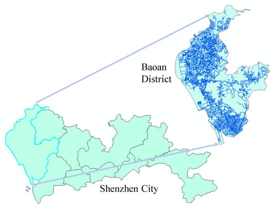
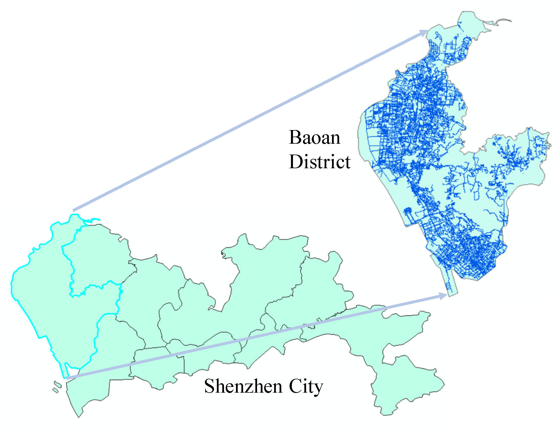
To demonstrate and verify the devised models and solution algorithms, we developed an ideal dataset (as presented in Figure 1, entitled [IDEAL]) with 12 spokes and four hubs and a dataset generated using the geography map of Baoan District, Shenzhen City, China, considering that Baoan should be a leading district for developing drone-based urban logistics system (see Figure 3). The Baoan District provides the environment for applying drones to instant delivery. The dataset is entitled $SaHbic$. For example, $S16H4i3$ is the ith dataset with 16 spokes and four hubs.

Figure 3. Shenzhen City and its Baoan District.

In [IDEAL], the coordinates of the nodes were regularly set to $\left[\mathrm{0,1},\mathrm{2,3},4\right]$. The distances among the nodes were calculated using Euclidean distance. Additional parameters were set to $\overline{H}=4,P^C=P^T=P^D=5,S^{truck}=S^{drone}=1,T^{order}=2.1$. and T^tr = 0.1.

The Baoan dataset was constructed using the following three steps. First, we obtained the geographical map from OpenStreetMap (www.openstreetmap.org, accessed on 4 June 2024). Second, we used the Baoan political polygon to extract the road network and catering positions from the map. Third, the spokes were randomly chosen from the merchant positions, and thus the datasets were generated.

We constructed the datasets based on actual data from Baoan District, Shenzhen City. The datasets are scalable; we can derive new ones from them by choosing nodes and connections. In the models and algorithms devised in Section 4 and Section 5, we focus on the distinct features of coupling HSN and drone technologies in the formulations and computational strategies while they do not impose particular assumptions on the datasets.

6.2. Assessment Metrics for Multi-Objective Optimization Solutions

We used three metrics, namely the number of non-dominated solutions (NS), hypervolume (HV), and Spacing, to assess the performance of multi-objective optimization algorithms. Each metric offers unique insights into different aspects of Pareto fronts, contributing to a comprehensive assessment of algorithmic effectiveness.

(1) The NS measures diversity, emphasizing the quantity and diversity of solutions on Pareto fronts [52]. The higher the NS, the broader the exploration of the Pareto fronts, facilitating the search for global optimal solutions.

(2) The HV measures the volume occupied by the non-dominated set, depicting the spatial coverage of non-dominated solutions, underscoring the convergence of solutions on Pareto fronts [53]. A larger HV is preferable in optimization problems with a minimization objective. The formula for calculating HV is formulated by Equation (24). The Lebesgue measure, denoted as $\delta \left(S\right)$, is employed to quantify the volume of the non-dominated solution set, representing its extent in the objective space; $\left|S\right|$ signifies the number of solutions in the non-dominated set; $v_i$ represents the HV formed by the reference point and the ith solution in the set.

$$\mathrm{Hypervolume} =\delta (S)-\sum _{i=1}^{\left|S\right|} v_i$$

(24)

(3) The Spacing metric quantifies the dispersion of solutions, capturing the relative distances between solutions [54]. Higher Spacing values imply a more favorable distribution of solutions, while lower values may indicate a concentration of the Pareto front solutions in specific local regions. Consequently, higher Spacing values are generally considered indicative of superior performance. The formula for calculating Spacing is as formulated by Equation (25), where $d_i$ represents the minimum distance from the ith solution to other solutions in the set $P,\left|P\right|$ denotes the number of solutions in set $P$, and $\bar{d}$ signifies the mean of all $d_i$.

$$\mathrm{S}\mathrm{p}\mathrm{a}\mathrm{c}\mathrm{i}\mathrm{n}\mathrm{g}(P)=\sqrt{\frac{1}{\left|P\right|}\sum _{i=1}^{\left|P\right|} {\left(d_i-\bar{d}\right)}^2}$$

(25)

6.3. Experimental Settings

In Table 4, we developed three groups of experiments to reveal the distinct features of the devised models and algorithms. In the first group, we compared the models and algorithms’ computing performances and optimality capabilities and determined the recommended values of the critical parameters. In the second group, we investigated the parameter sensitivities and impacts on computing performances. We examined four typical managerial strategies or scenarios in the third group, considering overdue delivery, rush hours, drone delays, and hub busyness and exploration.

Table 4. Experimental purposes, settings, and results.

No.	Purposes	Settings and Steps	Results
1	Demonstration	(1) Dataset: [IDEAL] (2) Models and algorithms: [M1],$\left[\mathrm{M}2\left(\epsilon =0.1\right)\right]$, [EAp], and [EAr].	Figure 4
2	Compare [M1] and [M2]	(1) Dataset: [S10H2i(0–9)]; 2) Models: [M1], [M2], and $\left[\mathrm{M}2\left(\epsilon =0.1\right)\right]$.	Table 5
3	Analyze the EA’s hyperparameters	(1) Dataset: [S60H6i0]; (2) Algorithms: [EAp] and [EAr].	Table 6
4	Compare [M2], [EAh] and [EAr]	(1) Dataset: [S10H3i1]; (2) Model: solve $\left[\mathrm{M}2\left(\epsilon \right)\right]$ for $\epsilon \in \left[\mathrm{0,0.1},\cdots \right]$ until there is no change in the objectives; (3) Algorithms: [EAp] and [EAr].	Figure 5
5	Compare [EAh] and [EAr]	(1) Dataset: [S(40, 60, 80, 100)H(4, 6, 8, 10)i0]; (2) Algorithms: [EAp] and [EAr].	Table 7 Figure 6
6	$\mathrm{Sensitivities} \mathrm{of} S^{truck}$$, S^{drone}$$, T^{order}$$, \mathrm{and} T^{tr}$	(1) Dataset: [S60H6i0]; (2) Algorithm: [EAr]; (3) The reference values of the four parameters: $\left[\mathrm{40.0,50.0,1.0,0.3}\right]$; (4) The ratios for adjusting the parameter values: $\left[-0.1,-\mathrm{0.05,0},\mathrm{0.05,0.10}\right]$;	Table 8 Figure 7
7	Number of hubs impacting on the performances	(1) Dataset: [S60H6i0]; (2) Algorithm: [EAr]; (3) Varying the hubs: $\overline{H}=\left[\mathrm{5,10},\cdots ,30\right]$.	Table 9 Figure 8
8	Number of spokes impacting on the performances	(1) Dataset: all datasets generated; (2) Algorithm: [EAr].	Table 10
9	Study the overdue delivery strategy	(1) Dataset: [S60H6i0]; (2) Algorithm: [EAr]; (3) The reference values of the order time $(T^{order}$): 1 h; (4) The ratios for adjusting the parameter values: $\left[\mathrm{0.00,0.05,0.10,0.15,0.20}\right]$.	Table 11 Figure 9
10	Impacts of urban rush hours on the solutions	(1) Dataset: [S60H6i0]; (2) Algorithm: [EAr]; (3) The reference values of the truck speed $(S^{truck}$): 50 km/h; (4) The ratios for adjusting the parameter values:$\left[0.00,-0.05,-0.10,-0.15,-0.20\right]$.	Table 12 Figure 10
11	Impacts of drone delays on the solutions	(1) Dataset: [S60H6i0]; (2) Algorithm: [EAr]; (3) The reference values of the drone speed $(S^{drone}$): 50 km/h; (4) The ratios for adjusting the parameter values: $\left[0.00,-0.05,-0.10,-0.15,-0.20\right]$.	Table 13 Figure 11
12	Impacts of hub busy and even explosion periods on the solutions	(1) Dataset: [S60H6i0]; (2) Algorithm: [EAr]; (3) The reference values of the hub stay time $(T^{tr}$): 0.3 h; (4) The ratios for adjusting the parameter values: $\left[\mathrm{0.00,0.05,0.10,0.15,0.20}\right]$.	Table 14 Figure 12

Figure 4. A demonstrative diagram of HSN.

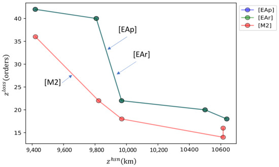
Figure 5. Pareto fronts of the results using [EAp], [EAr], and [M2].

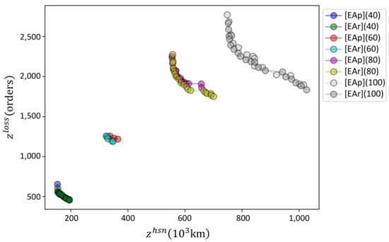
Figure 6. Pareto fronts of [EAp] and [EAr] used for solving four datasets.

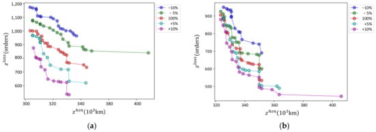
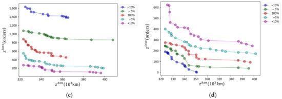
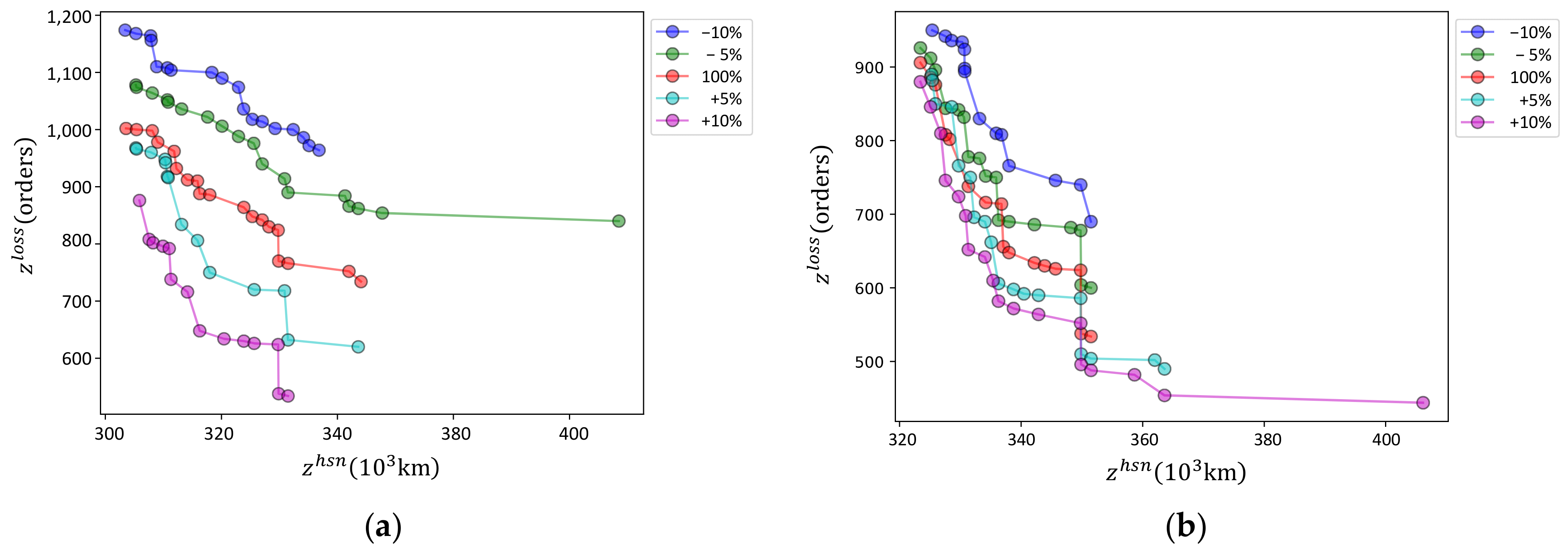
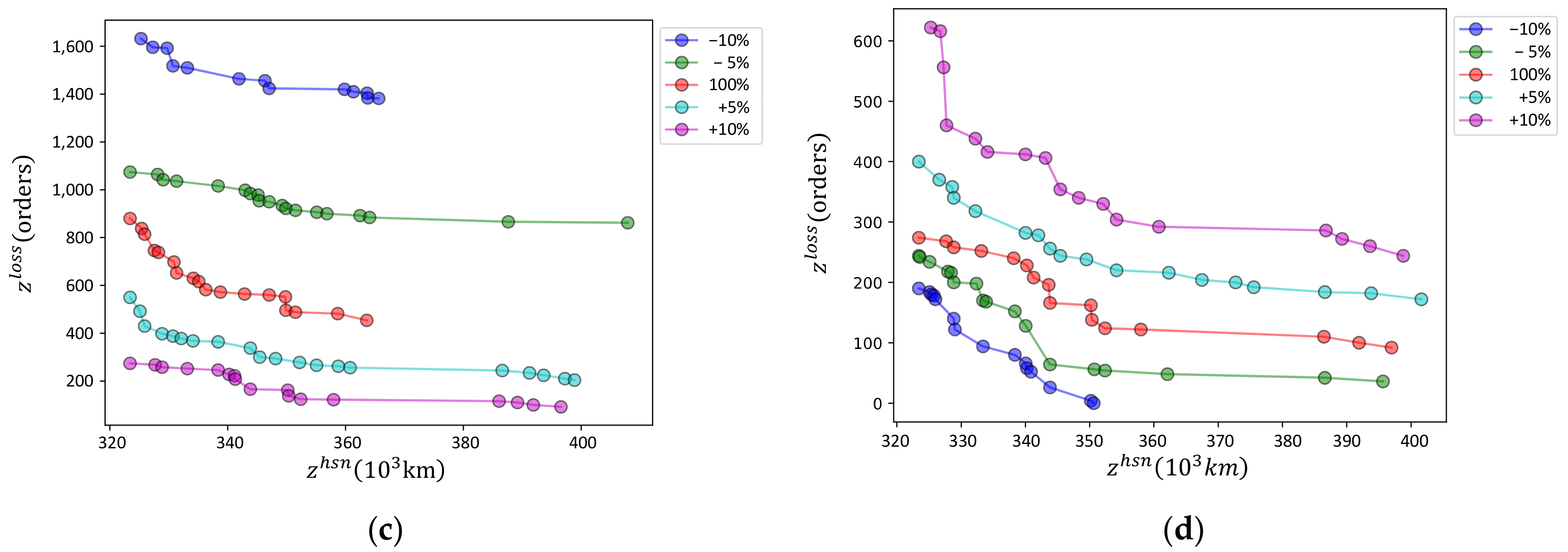
Figure 7. Pareto fronts of sensitivities of four parameters. (a) Truck speed; (b) Drone speeds; (c) Order time range; (d) Process time at hubs.

Figure 8. Pareto fronts of varying hub numbers.

Figure 9. Pareto fronts of extending order time overdue.

Figure 10. Pareto fronts impacted by truck speeds.

Figure 11. Pareto fronts impacted by drone delays in transportation.

Figure 12. Pareto fronts impacted by drone delays at hubs [S60H6i0].

Table 5. Objective values of solving [M1] and [M2].

Dataset	$\left[\mathbf{M}1\right]$	$\left[\mathbf{M}2\mathbf{a}\right]$		$\left[\mathbf{M}2\left(\mathit{\epsilon }=0.1\right)\right]$		$\frac{\left({\mathit{z}}^{\mathit{s}\mathit{u}\mathit{m}}-{\mathit{z}}^{\mathit{h}\mathit{s}\mathit{n}}\left(\mathit{\epsilon }\right)\right)\cdot 100}{{\mathit{z}}^{\mathit{s}\mathit{u}\mathit{m}}}$
	${\mathit{z}}^{\mathit{h}\mathit{s}\mathit{n}}$	${\mathit{z}}^{\mathit{h}\mathit{s}\mathit{n}}$	${\mathit{z}}^{\mathit{s}\mathit{u}\mathit{m}}$	${\mathit{z}}^{\mathit{h}\mathit{s}\mathit{n}}\left(\mathit{\epsilon }\right)$	${\mathit{z}}^{\mathit{s}\mathit{u}\mathit{m}}\left(\mathit{\epsilon }\right)$
S60H6i0	8361	8361	56	8361	26	53.57
S60H6i1	9421	9421	46	9421	36	21.74
S60H6i2	5740	5740	18	5740	18	0.00
S60H6i3	10,152	10,152	72	10,152	36	50.00
S60H6i4	9525	9525	84	9525	44	47.62
S60H6i5	9751	9751	42	9751	30	28.57
S60H6i6	9347	9347	48	9347	46	4.17
S60H6i7	11,439	11,439	78	11,439	52	33.33
S60H6i8	7999	7999	32	7999	32	0.00
S60H6i9	8333	8333	28	8333	26	7.14
Mean	9006.8	9006.8	50.4	9006.8	34.6	24.61

Table 6. Tuning the mutation and crossover probabilities of [EAp] and [EAr].

		[EAp]				[EAr]
		CT	HV	Spacing	NS	CT	HV	Spacing	NS
$p^m$	0.00	18.45	0.032	76.95	20	2.99	0.044	2050.63	16.54
	0.25	17.90	0.048	398.24	20	9.19	0.070	1644.33	18.74
	0.50	17.18	0.052	656.81	20	13.01	0.078	2395.58	18.66
	0.75	16.66	0.048	270.85	20	14.85	0.076	3889.27	16.06
	1.00	16.47	0.056	348.98	20	16.15	0.084	4738.29	14.08
$p^c$	0.00	17.67	0.042	31.81	20	9.77	0.062	3544.90	14.92
	0.25	17.42	0.046	358.84	20	10.78	0.070	2270.35	17.68
	0.50	17.68	0.046	340.67	20	11.48	0.072	2726.01	17.40
	0.75	16.90	0.050	586.60	20	11.98	0.074	2925.85	16.88
	1.00	17.00	0.052	433.91	20	12.18	0.074	3250.99	17.20

Note: CT = Computing time (s); HV = Hyper volume; NS = Number of Non-dominated solutions.

Table 7. Comparisons between [EAp] and [EAr].

	[EAp]				[EAr]
	CT	HV	Spacing	NS	CT	HV	Spacing	NS
S40H4i0	29.80	0.090	693.37	20	6.13	0.072	485.86	20
S60H6i0	66.84	0.018	0.00	20	33.09	0.020	1646.67	12
S80H8i0	109.64	0.052	2155.95	20	96.02	0.074	3145.04	20
S100H10i0	179.93	0.103	8278.05	20	176.28	0.102	7077.65	20

Note: CT = computing time (s); HV = hypervolume; NS = number of non-dominated solutions.

Table 8. Sensitivity analysis of $S^{truck},S^{drone},T^{order}$, and $T^{tr}$.

	${\mathit{S}}^{\mathit{t}\mathit{r}\mathit{u}\mathit{c}\mathit{k}}$					${\mathit{S}}^{\mathit{d}\mathit{r}\mathit{o}\mathit{n}\mathit{e}}$
	CT	HV	Spacing	NS		CT	HV	Spacing	NS
−10%	26.76	0.037	775.43	20	−10%	27.59	0.045	627.47	20
−5%	25.55	0.070	1213.59	20	−5%	27.41	0.056	678.49	20
40 km/h	28.79	0.052	703.80	20	50 km/h	34.00	0.063	840.17	20
+5%	42.30	0.066	2875.58	20	+5%	22.57	0.081	732.21	20
+10%	25.29	0.060	624.55	20	+10%	30.68	0.134	1588.44	20
	${\mathit{T}}^{\mathit{o}\mathit{r}\mathit{d}\mathit{e}\mathit{r}}$					${\mathit{T}}^{\mathit{t}\mathit{r}}$
	CT	HV	Spacing	NS		CT	HV	Spacing	NS
−10%	31.72	0.039	1090.38	20	−10%	27.72	0.130	661.56	20
−5%	37.62	0.065	5948.01	20	−5%	38.73	0.190	3331.42	18
1.0 h	30.01	0.087	1404.75	20	0.3 h	40.02	0.142	1453.31	20
+5%	39.60	0.147	976.20	20	+5%	41.18	0.136	2342.76	20

Note: CT = computing time (s); HV = hypervolume; NS = number of non-dominated solutions.

Table 9. Impacts of hubs on the solutions.

Hubs	CT	HV	Spacing	NS
5	20.26	0.120	873.76	20
10	58.55	0.135	2652.49	20
15	62.64	0.068	2613.29	19
20	65.15	0.016	255.07	6
25	67.16	0.025	6256.34	8

Note: CT = computing time (s); HV = hypervolume; NS = number of non-dominated solutions.

Table 10. Results of datasets with different spokes on the solution performances.

Dataset	Spokes	CT	HV	Spacing	NS
S10H2i(0–9)	10	0.52	0.021	198.67	9.0
S20H2i(0–9)	20	0.91	0.066	808.51	17.8
S30H3i(0–9)	30	2.13	0.084	362.13	20.0
S40H4i(0–9)	40	6.03	0.075	1349.72	18.9
S50H5i(0–9)	50	15.48	0.079	2150.26	20.0
S60H6i(0–9)	60	37.60	0.084	4649.13	19.7
S70H7i(0–9)	70	60.74	0.083	3728.19	19.8
S80H8i(0–9)	80	100.84	0.077	3447.47	19.9
S90H9i(0–9)	90	163.06	0.073	4785.11	20.0
S100H10i(0–9)	100	190.47	0.076	7020.31	19.9

Note: CT = computing time (s); HV = hypervolume; NS = number of non-dominated solutions.

Table 11. Impacts of overdue delivery on the solutions.

${\mathit{T}}^{\mathit{o}\mathit{r}\mathit{d}\mathit{e}\mathit{r}}/\mathbf{h}$	CT	HV	Spacing	NS
1.00	71.23	0.021	390.23	17
1.05	69.21	0.027	295.87	20
1.10	70.67	0.054	1480.62	18
1.15	70.43	0.072	823.20	17
1.20	74.54	0.072	5247.09	17

Note: CT = computing time (s); HV = hypervolume; NS = number of non-dominated solutions.

Table 12. Impacts of truck speeds on the solutions.

${\mathit{S}}^{\mathit{t}\mathit{r}\mathit{u}\mathit{c}\mathit{k}}/(\mathbf{k}\mathbf{m}/\mathbf{h})$	CT	HV	Spacing	NS
(50 km/h) -0%	74.44	0.061	1015.32	11
−5%	69.74	0.026	18,814.66	13
−10%	71.80	0.047	1663.90	16
−15%	70.61	0.058	3305.27	18
−20%	70.44	0.065	802.18	20

Note: CT = computing time (s); HV = hypervolume; NS = number of non-dominated solutions.

Table 13. Impacts of drone speeds on the solutions.

${\mathit{S}}^{\mathit{d}\mathit{r}\mathit{o}\mathit{n}\mathit{e}}/\left(\mathbf{k}\mathbf{m}/\mathbf{h}\right)$	CT	HV	Spacing	NS
(40 km/h) -0%	74.44	0.061	1015.32	11
−5%	69.74	0.026	18,814.66	13
−10%	71.80	0.047	1663.90	16
−15%	70.61	0.058	3305.27	18
−20%	70.44	0.065	802.18	20

Note: CT = computing time (s); HV = hypervolume; NS = number of non-dominated solutions.

Table 14. Impacts of busy hubs on the solutions.

${\mathit{T}}^{\mathit{t}\mathit{r}}/\mathbf{h}$	CT	HV	Spacing	NS
0.300 (+0.00%)	74.10	0.016	463.47	10
0.315 (+0.05%)	74.07	0.017	178.23	13
0.330 (+0.10%)	77.26	0.013	636.95	6
0.345 (+0.15%)	79.38	0.013	338.28	9
0.360 (+0.20%)	82.33	0.013	128.00	9

Note: CT = computing time (s); HV = hypervolume; NS = number of non-dominated solutions.

Table 4. Experimental purposes, settings, and results.

No.	Purposes	Settings and Steps	Results
1	Demonstration	(1) Dataset: [IDEAL] (2) Models and algorithms: [M1],$\left[\mathrm{M}2\left(\epsilon =0.1\right)\right]$, [EAp], and [EAr].	Figure 4
2	Compare [M1] and [M2]	(1) Dataset: [S10H2i(0–9)]; 2) Models: [M1], [M2], and $\left[\mathrm{M}2\left(\epsilon =0.1\right)\right]$.	Table 5
3	Analyze the EA’s hyperparameters	(1) Dataset: [S60H6i0]; (2) Algorithms: [EAp] and [EAr].	Table 6
4	Compare [M2], [EAh] and [EAr]	(1) Dataset: [S10H3i1]; (2) Model: solve $\left[\mathrm{M}2\left(\epsilon \right)\right]$ for $\epsilon \in \left[\mathrm{0,0.1},\cdots \right]$ until there is no change in the objectives; (3) Algorithms: [EAp] and [EAr].	Figure 5
5	Compare [EAh] and [EAr]	(1) Dataset: [S(40, 60, 80, 100)H(4, 6, 8, 10)i0]; (2) Algorithms: [EAp] and [EAr].	Table 7 Figure 6
6	$\mathrm{Sensitivities} \mathrm{of} S^{truck}$$, S^{drone}$$, T^{order}$$, \mathrm{and} T^{tr}$	(1) Dataset: [S60H6i0]; (2) Algorithm: [EAr]; (3) The reference values of the four parameters: $\left[\mathrm{40.0,50.0,1.0,0.3}\right]$; (4) The ratios for adjusting the parameter values: $\left[-0.1,-\mathrm{0.05,0},\mathrm{0.05,0.10}\right]$;	Table 8 Figure 7
7	Number of hubs impacting on the performances	(1) Dataset: [S60H6i0]; (2) Algorithm: [EAr]; (3) Varying the hubs: $\overline{H}=\left[\mathrm{5,10},\cdots ,30\right]$.	Table 9 Figure 8
8	Number of spokes impacting on the performances	(1) Dataset: all datasets generated; (2) Algorithm: [EAr].	Table 10
9	Study the overdue delivery strategy	(1) Dataset: [S60H6i0]; (2) Algorithm: [EAr]; (3) The reference values of the order time $(T^{order}$): 1 h; (4) The ratios for adjusting the parameter values: $\left[\mathrm{0.00,0.05,0.10,0.15,0.20}\right]$.	Table 11 Figure 9
10	Impacts of urban rush hours on the solutions	(1) Dataset: [S60H6i0]; (2) Algorithm: [EAr]; (3) The reference values of the truck speed $(S^{truck}$): 50 km/h; (4) The ratios for adjusting the parameter values:$\left[0.00,-0.05,-0.10,-0.15,-0.20\right]$.	Table 12 Figure 10
11	Impacts of drone delays on the solutions	(1) Dataset: [S60H6i0]; (2) Algorithm: [EAr]; (3) The reference values of the drone speed $(S^{drone}$): 50 km/h; (4) The ratios for adjusting the parameter values: $\left[0.00,-0.05,-0.10,-0.15,-0.20\right]$.	Table 13 Figure 11
12	Impacts of hub busy and even explosion periods on the solutions	(1) Dataset: [S60H6i0]; (2) Algorithm: [EAr]; (3) The reference values of the hub stay time $(T^{tr}$): 0.3 h; (4) The ratios for adjusting the parameter values: $\left[\mathrm{0.00,0.05,0.10,0.15,0.20}\right]$.	Table 14 Figure 12

6.4. Results

As presented in Table 4 for the 12 experiments, the results with figures, tables, and explanations are given in the following sub-section.

6.4.1. Demonstration

The devised models and algorithms solve the dataset [IDEAL] and get the same results as Figure 4. This dataset is typically ideal, and its Pareto front has only one solution. In the solution, $z^{hsn}=874$ and $z^{loss}=216$; namely, there are 216 orders whose engagement times are beyond $T^{order}$. For example, because $T^{order}=2.1$, the order $\left(i=13,j=5\right)$ with direct distance 2 will not be met because the drone-based instant delivery distance contains five parts, $13\to 10\to 6\to 5$. The distance is beyond 2 because there is additional processing time at hubs 10 and 6.

6.4.2. Compare [M1] and [M2]

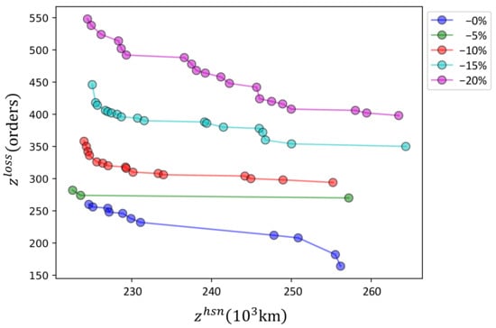
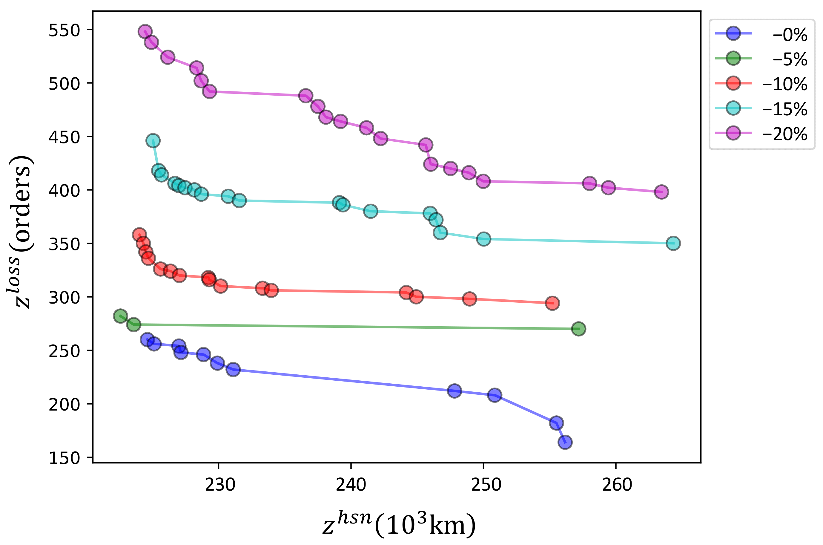
As studied in Section 4, [M1] is a baseline HSN optimization model, while the extended [M2] optimizes the logistics cost and order loss in the bi-objective program. As revealed in Table 5, [M2a] minimizes $z^{hsn}$ and so gets the same results as [M1]. The model $\left[\mathrm{M}2\left(\epsilon =0.1\right)\right]$ relaxes the objective $z^{hsn}$ by 10% and then minimizes $z^{loss}$. We can find that the unmet orders are significantly reduced by 24.61% on average.

6.4.3. Analyze the Hyperparameters of [EAp] and [EAr]

Table 6 presents the results of crossing experiments on the mutation probability ($P^m$) and the crossover probability ($P^c$). Here, $P^m$ and $P^c$ iterate five values, $\left[\mathrm{0,0.25,0.5,0.5,1}\right]$, and we calculate four metrics, namely computing time (CT), hypervolume (HV), Spacing, and the number of non-dominated solutions (NS). We cannot recommend concrete values based on the experimental results because four metrics are involved. However, we can judge that bigger values are more beneficial than minor ones. We set $P^m$ to 0.25 and $P^c$ to 1.00 in the following experiments.

6.4.4. Compare [M2], [EAp], and [EAr]

When solving instances with more spokes (beyond 20), [M1] and [M2] cannot obtain optimal solutions within an acceptable time. In Figure 5, [M2], [EAp], and [EAr] can obtain solutions, while [M2] can obtain better Pareto fronts than [EAp] and [EAr]. In this case, [EAp] and [EAr] obtain the same Pareto front. Although [M2] with $\epsilon$-constraints may find better Pareto fronts, it fails to solve even medium-scale instances. Therefore, we devised [EAp] and [EAr] for medium- and large-scale HSN instances.

6.4.5. Compare [EAp] and [EAr]

Two EAs, [EAp] and [EAr], were devised considering two different encoding/decoding schemes. [EAp] uses individuals with genes of the same length as spokes and encodes them as permutations of spoke indices. [EAr] maps $2\overline{H}$ and keys as coordinates to hubs. So, [EAr] uses fewer genes for solutions. In Table 7, the computing time of [EAr] is less than [EAp]; as for HV and Space, [EAr] is also competitive, while the NS values are not stable. In Figure 6, [EAr] can generate a better Pareto front than [EAp], although the competitiveness is minor. Comprehensively, [EAr] is chosen as the algorithm in the following experiments.

6.4.6. Sensitivities of Four Parameters

As studied in Section 4, the drone-based HSN will be affected much by the key parameters, including $S^{truck},S^{drone},T^{order}$, and $T^{tr}$. As shown in Table 8, the computing time (CT) is unstable for all the parameters and variations; the number of non-denominated solutions (NS) is stable and can obtain enough. The Spacing metrics also incur uncertainties while the trends are apparent. The impacts on HV are clear. Figure 7 gives five Pareto fronts ($-10\%,-5\%,0\%,+5\%,10\%$) for each parameter’s sensitivity analysis results.

6.4.7. Numbers of Hubs Impacting on the Performances

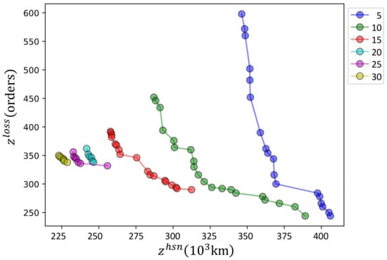
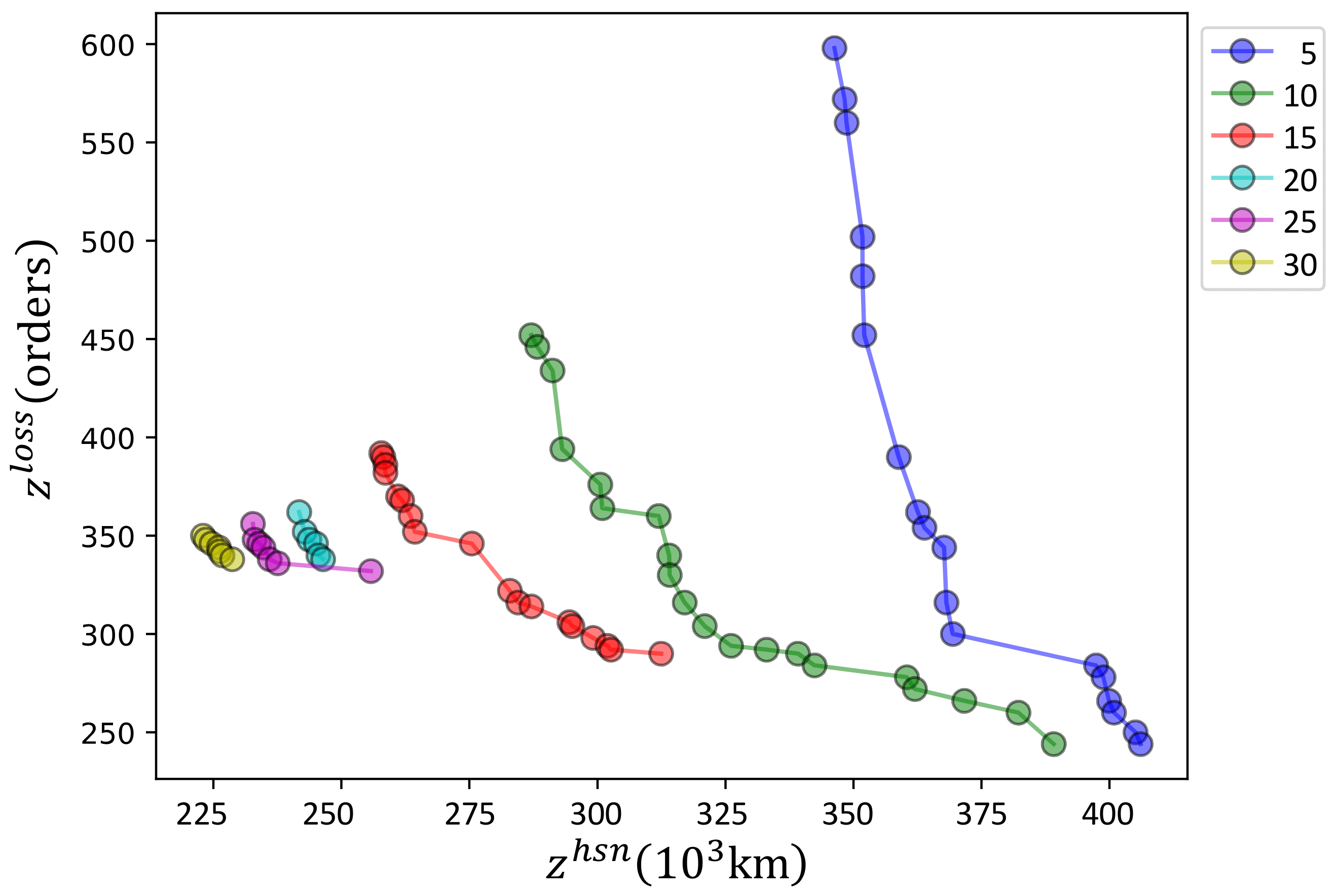
[EAr] uses $2\overline{H}$ individuals in the encoding and decoding schemes so that the hubs will impact the solution performances. In Table 9, when increasing the number of hubs (NS), the computing time (CT) decreases, the HV and NS values also lower with a tendency, while the Space metrics are not stable. In Figure 8, from five to 10 hubs, the Pareto front moves to the corner fast.

6.4.8. Numbers of Spokes Impacting on the Performances

As studied above, the number of hubs can affect the HSN solution difficulty, while Table 10 indicates that the number of spokes is the most affected. The computing time (CT) drastically increases when the number of spokes (NS) increases from 10 to 100. In Spacing metrics, more spokes help find diversities of solutions on the Pareto fronts.

6.4.9. Study the Overdue Delivery Strategy

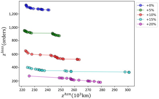
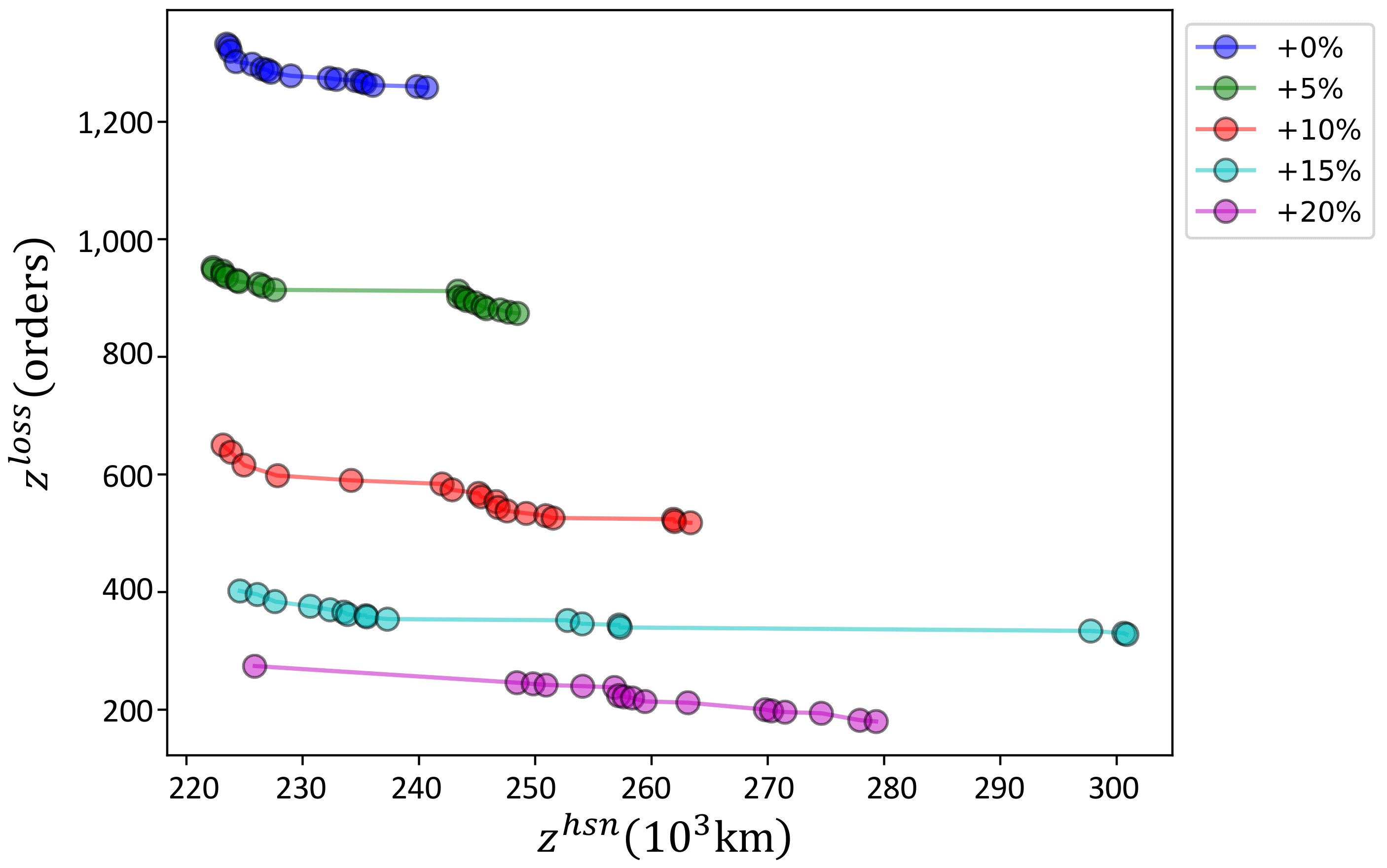
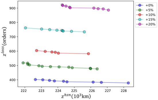
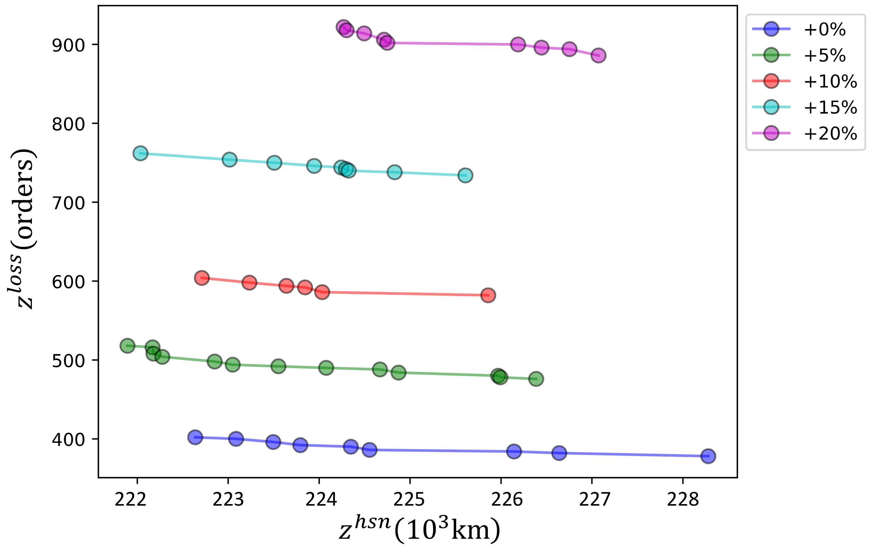
In drone-based instant delivery, the merchants should have a strong attitude to extend the acceptable order engagement time range ($T^{order}$) because it will enlarge the coverage of the transshipment hubs and the consumer group. However, they must consider the costs to extend the overdue delivery. Consumers may accept comparatively delayed delivery for three reasons: first, drone-based delivery is fantastic; second, drone-based delivery is much cleaner and contactless; third, it is at least a new choice. Table 11 presents the results of increasing $T^{order}$, and Figure 9 depicts five Pareto fronts. From 0% to 5% and 5% to 10%, the Pareto front moves fast.

6.4.10. Impacts of Urban Rush Hours on the Solutions

Big cities generally have several rush hours, which will affect the truck speeds in the transshipment stage.

6.4.11. Impacts of Drone Delays on the Solutions

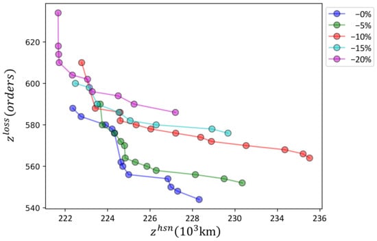
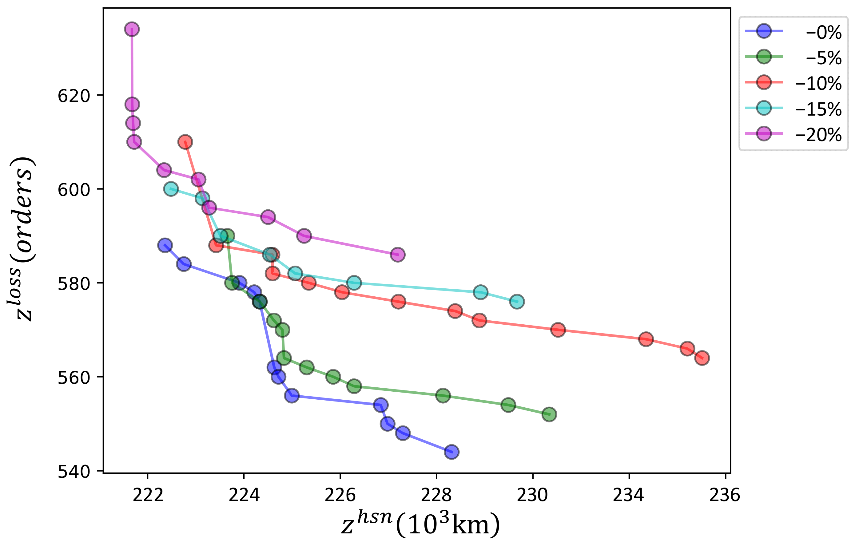
The drones may delay transportation because of air and various emergency conditions. Although the reasons may be diverse, the impacts on the logistics are mainly reflected by reduced drone speeds. Table 13 shows the results of gradually reducing drone speeds. Figure 11 further depicts the Pareto fronts. In the illustrated case, a slight delay (5%) may be acceptable, and a 10% delay is severe.

6.4.12. Impacts of Busy Hubs and Even Explosion Periods on the Solutions

In [M2], the busy hubs and explosion degrees are formulated by the parameter $T^{tr}$, which depends on the efficiency of transshipment at the hubs. Table 14 presents the impacts of the four performance metrics by increasing $T^{tr}$. When its value is tight, CT increases, HV drops, and NS drops, making it difficult to find solutions. Figure 12 indicates that bigger $T^{tr}$ values will drastically make more unmet orders.

6.5. Managerial Implications

Based on the results analyzed above for the devised models and algorithms, we can conclude that the following generations have managerial implications for drone-based instant delivery service providers and merchants.

(1) Drone-based pickup and delivery can utilize the economy of scale of transportation while additional interaction time is incurred, including the processing times at hubs, transshipment operations between drones and trucks, and drones and loading/unloading cabinets (Section 6.4).

(2) Introducing drones for urban instant pickup and delivery may prolong the order engagement time. Optimizing the logistics networks and tuning the parameters can help reduce costs and mitigate order losses (Section 6.4.9).

(3) HSN and extended HSN optimization, particularly when considering urban drone-based instant delivery, pose challenges for on-the-shelf mathematical program solvers. As examined in Section 6, mathematical programs can produce good Pareto fronts for small-scale instances, while [EAr] and [EAp] are competitive in solving large-scale instances and cannot ensure optimality. It is practical to develop heuristics and intelligent algorithms (Section 6.4.4 and Section 6.4.5).

(4) More hubs will demand more computing resources and challenge the solution methods. More hubs could be practical in drone-based instant delivery, given that transshipment hubs should be more flexible than traditional city logistics (Section 6.4.7 and Section 6.4.8).

(5) Practical applications of the devised models and algorithms must address large-scale instances, e.g., with more than 100 spokes. So, fast solution algorithms with promising computing performance are essential (Section 6.4.4 and Section 6.4.5).

(6) Multi-objective Pareto front analysis assesses the impacts of extending the order engagement time ranges on the solutions, which must reflect the costs. So, drone-based instant delivery service providers and merchants should prioritize balancing expenses and revenues (from Section 6.4.7, Section 6.4.8, Section 6.4.9, Section 6.4.10, Section 6.4.11 and Section 6.4.12).

(7) The Pareto front analysis of the drone delays can contribute to investing and backing up additional drones. Drone-based instant delivery service providers should carefully weigh the Pareto front improvement and drone investment costs (from Section 6.4.7, Section 6.4.8, Section 6.4.9, Section 6.4.10, Section 6.4.11 and Section 6.4.12).

(8) Among all parameters and strategies, mitigating drone delays at hubs may impact the solution most, and addressing it is achievable through effective management, advanced technologies, and innovations (Section 6.4).

7. Conclusions

Drone-based instant delivery with simultaneous first and last-mile pickup is a challenging decision-making and optimization problem. Inspired by the Shenzhen City drone-based instant delivery case, this study investigated the hub-and-spoke network (HSN) optimization problem, considering logistics costs and order loss minimization as a bi-objective optimization problem. Extending the baseline HSN model, we devised a bi-objective mixed-integer linear program (MILP), solved by the $\epsilon$-constraint method and two evolutionary algorithms using permutation (EAp) and rand keys (EAr) as encoding and decoding schemes. Using an ideal dataset and the datasets generated in the Shenzhen City scenarios, the solution methods are compared by experiments, the parameter sensitivities are analyzed numerically, and three groups and twelve experiments are conducted to demonstrate the problem features and validate the devised models and algorithms.

The examined drone-based logistics networks and operations optimization problems are exciting and challenging in formulation and algorithm development. Based on the problem and the methods devised, the following research directions should help enable the development of drone-based instant delivery. First, extending the solution algorithms by mathematic heuristics and advanced intelligent algorithms for large-scale practical instances is beneficial. For example, the Baoan District of Shenzhen City contains more than 20,000 takeaway merchants and 200,000 buildings. The existing algorithms based on NSGA-II can be adapted to other multi-objective optimization algorithms that may optimize computation performance and optimality. Further, we will try to find solutions to the multi-objective model by using methods that solve mathematical programs exactly. Second, the instant delivery scenarios are full of uncertainties and dynamics. We should extend the deterministic solutions to stochastic programs and robust optimization. We can even incorporate the potential economic and environmental impacts of widespread drone use in urban logistics into the models. Third, some cities are trying different logistics service modes. The layouts and traffic conditions of other cities may also impact network optimization and scheduling results, and thus, it is beneficial to develop dataset generation schemes. We can create the mode featured by drone-based pickup/delivery and truck-based transshipment to other creative modes, e.g., crowdsourcing and cloud logistics.

References

- Ghelichi, Z.; Gentili, M.; Mirchandani, P.B. Drone logistics for uncertain demand of disaster-impacted populations. Transp. Res. Part C-Emerg. Technol. 2022, 141, 103735. [Google Scholar] [CrossRef] [Scilit]
- Bonini, T.; Treré, E.; Yu, Z.Z.; Singh, S.; Cargnelutti, D.; López-Ferrández, F.J. Cooperative affordances: How instant messaging apps afford learning, resistance and solidarity among food delivery workers. Convergence 2023, 30, 554–571. [Google Scholar] [CrossRef] [Scilit]
- Zhao, Y.L.; Cattaruzza, D.; Kang, N.X.; Roberti, R. Synchronized Deliveries with a Bike and a Self-Driving Robot. Transp. Sci. 2024, 58, 219–239. [Google Scholar] [CrossRef] [Scilit]
- Leon, S.; Chen, C.; Ratcliffe, A. Consumers’ perceptions of last mile drone delivery. Int. J. Logist. Res. Appl. 2023, 26, 345–364. [Google Scholar] [CrossRef] [Scilit]
- Janke, C.; de Haag, M.U. Implementation of European Drone Regulations-Status Quo and Assessment. J. Intell. Robot. Syst. 2022, 106, 33. [Google Scholar] [CrossRef] [Scilit]
- Sawadsitang, S.; Niyato, D.; Tan, P.S.; Wang, P.; Nutanong, S. Shipper Cooperation in Stochastic Drone Delivery: A Dynamic Bayesian Game Approach. IEEE Trans. Veh. Technol. 2021, 70, 7437–7452. [Google Scholar] [CrossRef] [Scilit]
- Macias, J.E.; Angeloudis, P.; Ochieng, W. Optimal hub selection for rapid medical deliveries using unmanned aerial vehicles. Transp. Res. Part C-Emerg. Technol. 2020, 110, 56–80. [Google Scholar] [CrossRef] [Scilit]
- Majd, A.; Loni, M.; Sahebi, G.; Daneshtalab, M. Improving Motion Safety and Efficiency of Intelligent Autonomous Swarm of Drones. Drones 2020, 4, 48. [Google Scholar] [CrossRef] [Scilit]
- Lappas, V.; Zoumponos, G.; Kostopoulos, V.; Lee, H.I.; Shin, H.S.; Tsourdos, A.; Tantardini, M.; Shomko, D.; Munoz, J.; Amoratis, E.; et al. EuroDRONE, a European Unmanned Traffic Management Testbed for U-Space. Drones 2022, 6, 53. [Google Scholar] [CrossRef] [Scilit]
- Smith, A.; Dickinson, J.E.; Marsden, G.; Cherrett, T.; Oakey, A.; Grote, M. Public acceptance of the use of drones for logistics: The state of play and moving towards more informed debate. Technol. Soc. 2022, 68, 101883. [Google Scholar] [CrossRef] [Scilit]
- Bruni, M.E.; Khodaparasti, S.; Moshref-Javadi, M. A logic-based Benders decomposition method for the multi-trip traveling repairman problem with drones. Comput. Oper. Res. 2022, 145, 105845. [Google Scholar] [CrossRef] [Scilit]
- Huang, H.L.; Savkin, A.V.; Huang, C. Reliable Path Planning for Drone Delivery Using a Stochastic Time-Dependent Public Transportation Network. IEEE Trans. Intell. Transp. Syst. 2021, 22, 4941–4950. [Google Scholar] [CrossRef] [Scilit]
- Meng, Z.Y.; Zhou, Y.T.; Li, E.Y.; Peng, X.Y.; Qiu, R. Environmental and economic impacts of drone-assisted truck delivery under the carbon market price. J. Clean. Prod. 2023, 401, 136758. [Google Scholar] [CrossRef] [Scilit]
- Huang, H.L.; Savkin, A.V. Deployment of Charging Stations for Drone Delivery Assisted by Public Transportation Vehicles. IEEE Trans. Intell. Transp. Syst. 2022, 23, 15043–15054. [Google Scholar] [CrossRef] [Scilit]
- Fehling, C.; Saraceni, A. Technical and legal critical success factors: Feasibility of drones & AGV in the last-mile-delivery. Transp. Bus. Manag. 2023, 50, 101029. [Google Scholar]
- Zhen, L.; Wu, J.W.; Laporte, G.; Tan, Z.Y. Heterogeneous instant delivery orders scheduling and routing problem. Comput. Oper. Res. 2023, 157, 106246. [Google Scholar] [CrossRef] [Scilit]
- Gu, Q.C.; Fan, T.J.; Pan, F.; Zhang, C. A vehicle-UAV operation scheme for instant delivery. Comput. Ind. Eng. 2020, 149, 106809. [Google Scholar] [CrossRef] [Scilit]
- Guo, C.J.; Thompson, R.G.; Foliente, G.; Peng, X.S. Reinforcement learning enabled dynamic bidding strategy for instant delivery trading. Comput. Ind. Eng. 2021, 160, 107596. [Google Scholar] [CrossRef] [Scilit]
- Chauhan, D.R.; Unnikrishnan, A.; Boyles, S.D. Maximum Profit Facility Location and Dynamic Resource Allocation for Instant Delivery Logistics. Transp. Res. Rec. 2022, 2676, 697–710. [Google Scholar] [CrossRef] [Scilit]
- Chen, J.Y.; Fan, T.J.; Gu, Q.C.; Pan, F. Emerging technology-based online scheduling for instant delivery in the O2O retail era. Electron. Commer. Res. Appl. 2022, 51, 101115. [Google Scholar] [CrossRef] [Scilit]
- Cui, S.X.; Sun, Q.; Zhang, Q. A Time-Dependent Vehicle Routing Problem for Instant Delivery Based on Memetic Algorithm. Comput. Intell. Neurosci. 2022, 2022, 5099008. [Google Scholar] [CrossRef] [Scilit] [PubMed]
- Hou, Y.; Guo, X.Y.; Han, H.G.; Wang, J.J. Knowledge-driven ant colony optimization algorithm for vehicle routing problem in instant delivery peak period. Appl. Soft Comput. 2023, 145, 110551. [Google Scholar] [CrossRef] [Scilit]
- Snoeck, A.; Winkenbach, M.; Fransoo, J.C. On-demand last-mile distribution network design with omnichannel inventory. Transp. Res. Part E-Logist. Transp. Rev. 2023, 180, 103324. [Google Scholar] [CrossRef] [Scilit]
- Wu, J.; Zhang, P.W.; Wang, Y.; Shi, J.M. Integrated aviation model and metaheuristic algorithm for hub-and-spoke network design and airline fleet planning. Transp. Res. Part E-Logist. Transp. Rev. 2022, 164, 102755. [Google Scholar] [CrossRef] [Scilit]
- Zhou, S.Q.; Ji, B.; Song, Y.L.; Yu, S.S.; Zhang, D.Z.; Van Woensel, T. Hub-and-spoke network design for container shipping in inland waterways. Expert Syst. Appl. 2023, 223, 119850. [Google Scholar] [CrossRef] [Scilit]
- Zheng, J.F.; Meng, Q.; Sun, Z. Liner hub-and-spoke shipping network design. Transp. Res. Part E-Logist. Transp. Rev. 2015, 75, 32–48. [Google Scholar] [CrossRef] [Scilit]
- Arbabi, H.; Nasiri, M.M.; Bozorgi-Amiri, A. A hub-and-spoke architecture for a parcel delivery system using the cross-docking distribution strategy. Eng. Optim. 2021, 53, 1593–1612. [Google Scholar] [CrossRef] [Scilit]
- Jeong, S.J.; Lee, C.G.; Bookbinder, J.H. The European freight railway system as a hub-and-spoke network. Transp. Res. Part A-Policy Pract. 2007, 41, 523–536. [Google Scholar] [CrossRef] [Scilit]
- De Freitas, C.C.; Aloise, D.J.; Fontes, F.F.D.; Santos, A.C.; Menezes, M.D. A biased random-key genetic algorithm for the two-level hub location routing problem with directed tours. OR Spectr. 2023, 45, 903–924. [Google Scholar] [CrossRef] [Scilit]
- Kemmar, O.; Bouamrane, K.; Gelareh, S. Hub location problem in round-trip service applications. Rairo-Oper. Res. 2021, 55, S2831–S2858. [Google Scholar] [CrossRef] [Scilit]
- Li, Z.C.; Bing, X.; Fu, X.W. A hierarchical hub location model for the integrated design of urban and rural logistics networks under demand uncertainty. Ann. Oper. Res. 2023. [Google Scholar] [CrossRef] [Scilit] [PubMed]
- Hu, Q.M. A reconfiguration optimisation model for hub-and-spoke network mergers. Eur. J. Ind. Eng. 2017, 11, 101–132. [Google Scholar] [CrossRef] [Scilit]
- Pirkul, H.; Schilling, D.A. An efficient procedure for designing single allocation hub and spoke systems. Manag. Sci. 1998, 44, S235–S242. [Google Scholar] [CrossRef] [Scilit]
- Gelareh, S.; Nickel, S.; Pisinger, D. Liner shipping hub network design in a competitive environment. Transp. Res. Part E-Logist. Transp. Rev. 2010, 46, 991–1004. [Google Scholar] [CrossRef] [Scilit]
- Zhao, L.; Bi, X.H.; Dong, Z.H.; Xiao, N.; Zhao, A.N. Robust traveling salesman problem with drone: Balancing risk and makespan in contactless delivery. Int. Trans. Oper. Res. 2024, 31, 167–191. [Google Scholar] [CrossRef] [Scilit]
- Zhu, T.K.; Boyles, S.D.; Unnikrishnan, A. Two-stage robust facility location problem with drones. Transp. Res. Part C-Emerg. Technol. 2022, 137, 103563. [Google Scholar] [CrossRef] [Scilit]
- Salama, M.R.; Srinivas, S. Collaborative truck multi-drone routing and scheduling problem: Package delivery with flexible launch and recovery sites. Transp. Res. Part E-Logist. Transp. Rev. 2022, 164, 102788. [Google Scholar] [CrossRef] [Scilit]
- Zou, B.P.; Wu, S.Q.; Gong, Y.M.; Yuan, Z.; Shi, Y.Q. Delivery network design of a locker-drone delivery system. Int. J. Prod. Res. 2023, 62, 4097–4121. [Google Scholar] [CrossRef] [Scilit]
- Li, H.Q.; Chen, J.; Wang, F.L.; Zhao, Y.B. Truck and drone routing problem with synchronization on arcs. Nav. Res. Logist. 2022, 69, 884–901. [Google Scholar] [CrossRef] [Scilit]
- Yin, Y.Q.; Yang, Y.J.; Yu, Y.G.; Wang, D.J.; Cheng, T. Robust vehicle routing with drones under uncertain demands and truck travel times in humanitarian logistics. Transp. Res. Part B-Methodol. 2023, 174, 102781. [Google Scholar] [CrossRef] [Scilit]
- Kim, D.; Lee, K.; Moon, I. Stochastic facility location model for drones considering uncertain flight distance. Ann. Oper. Res. 2019, 283, 1283–1302. [Google Scholar] [CrossRef] [Scilit]
- Shi, Z. Shenzhen Is Piloting a New Model of Drone Delivery for Takeout. Available online: https://www.thepaper.cn/newsDetail_forward_23169009 (accessed on 6 February 2024).
- Shen, L.; Wang, Y.; Liu, K.; Yang, Z.; Shi, X.; Yang, X.; Jing, K. Synergistic path planning of multi-UAVs for air pollution detection of ships in ports. Transp. Res. Part E Logist. Transp. Rev. 2020, 144, 102128. [Google Scholar] [CrossRef] [Scilit]
- Shen, L.; Hou, Y.; Yang, Q.; Lv, M.; Dong, J.-X.; Yang, Z.; Li, D. Synergistic path planning for ship-deployed multiple UAVs to monitor vessel pollution in ports. Transp. Res. Part D Transp. Environ. 2022, 110, 103415. [Google Scholar] [CrossRef] [Scilit]
- Borghetti, F.; Caballini, C.; Carboni, A.; Grossato, G.; Maja, R.; Barabino, B. The Use of Drones for Last-Mile Delivery: A Numerical Case Study in Milan, Italy. Sustainability 2022, 14, 1766. [Google Scholar] [CrossRef] [Scilit]
- Deb, K.; Pratap, A.; Agarwal, S.; Meyarivan, T. A fast and elitist multiobjective genetic algorithm: NSGA-II. IEEE Trans. Evol. Comput. 2002, 6, 182–197. [Google Scholar] [CrossRef] [Scilit]
- Jensen, M.T. Reducing the run-time complexity of multiobjective EAs: The NSGA-II and other algorithms. IEEE Trans. Evol. Comput. 2003, 7, 503–515. [Google Scholar] [CrossRef] [Scilit]
- Srinivas, N.; Deb, K. Muiltiobjective Optimization Using Nondominated Sorting in Genetic Algorithms. Evol. Comput. 1994, 2, 221–248. [Google Scholar] [CrossRef] [Scilit]
- Deng, W.; Zhang, X.; Zhou, Y.; Liu, Y.; Zhou, X.; Chen, H.; Zhao, H. An enhanced fast non-dominated solution sorting genetic algorithm for multi-objective problems. Inf. Sci. 2022, 585, 441–453. [Google Scholar] [CrossRef] [Scilit]
- Yahyaoui, H.; Kaabachi, I.; Krichen, S.; Dekdouk, A. Two metaheuristic approaches for solving the multi-compartment vehicle routing problem. Oper. Res. 2020, 20, 2085–2108. [Google Scholar] [CrossRef] [Scilit]
- Lin, Q.Z.; Chen, J.Y.; Zhan, Z.H.; Chen, W.N.; Coello, C.A.C.; Yin, Y.L.; Lin, C.M.; Zhang, J. A Hybrid Evolutionary Immune Algorithm for Multiobjective Optimization Problems. IEEE Trans. Evol. Comput. 2016, 20, 711–729. [Google Scholar] [CrossRef] [Scilit]
- Tian, Y.; Cheng, R.; Zhang, X.Y.; Li, M.Q.; Jin, Y.C. Diversity Assessment of Multi-Objective Evolutionary Algorithms: Performance Metric and Benchmark Problems. IEEE Comput. Intell. Mag. 2019, 14, 61–74. [Google Scholar] [CrossRef] [Scilit]
- Zapotecas-Martinez, S.; Lopez-Jaimes, A.; Garcia-Najera, A. LIBEA: A Lebesgue Indicator-Based Evolutionary Algorithm for multi-objective optimization. Swarm Evol. Comput. 2019, 44, 404–419. [Google Scholar] [CrossRef] [Scilit]
- Kumar, S.; Tejani, G.G.; Pholdee, N.; Bureerat, S. Multi-objective modified heat transfer search for truss optimization. Eng. Comput. 2021, 37, 3439–3454. [Google Scholar] [CrossRef] [Scilit]
Disclaimer/Publisher’s Note: The statements, opinions and data contained in all publications are solely those of the individual author(s) and contributor(s) and not of MDPI and/or the editor(s). MDPI and/or the editor(s) disclaim responsibility for any injury to people or property resulting from any ideas, methods, instructions or products referred to in the content. |
© 2024 by the authors. Licensee MDPI, Basel, Switzerland. This article is an open access article distributed under the terms and conditions of the Creative Commons Attribution (CC BY) license (https://creativecommons.org/licenses/by/4.0/).