Egocentric Constraint Corridor: Deep Reinforcement Learning for Fixed-Wing UAV Navigation in Vertically Constrained Airspace

Highlights

What are the main findings?

• We propose the Egocentric Constraint Corridor representation, which fuses heterogeneous multi-source constraints into a constraint corridor and encodes it as an egocentric margin field serving as the navigation policy’s observation input, and ablation studies show that this margin field is a necessary condition for reliable corridor navigation: removing it reduces the success rate from 94.0% to 22.7%.
• The deep reinforcement learning navigation policy built on this representation relies solely on local observations, achieving a path efficiency of 0.866 that approaches the globally informed A* (0.942) and exceeds that of Dubins-RRT* (0.738).

What are the implications of the main findings?

• Egocentric encoding makes the margin field depend only on the relative geometry between the vehicle and the surrounding corridor; geometrically similar corridor segments produce consistent observations regardless of their global location, enabling the trained policy to transfer zero-shot to unseen terrains and radar deployments without retraining or fine-tuning.
• The complete observation construction and policy inference pipeline achieves a maximum end-to-end latency of 10.17 ms on an embedded platform, well below the 200 ms decision interval, and hardware-in-the-loop experiments verify the feasibility of real-time closed-loop operation.

Abstract

Fixed-wing UAVs operating in long-range missions often fly through airspace subject to heterogeneous multi-source constraints that vertically compress the flyable space into a constraint corridor of continuously varying thickness. Conventional path planning methods incur high online computational costs in such scenarios. Deep reinforcement learning can generate reactive decisions from local observations, yet existing approaches predominantly target multirotor obstacle avoidance and rely on observations designed for discrete obstacles, lacking a unified representation for corridor constraints. Moreover, constraint conditions vary across mission scenarios, demanding cross-scenario policy generalization. This paper proposes the Egocentric Constraint Corridor (ECC), which fuses multi-source constraints into upper and lower boundary surfaces defining the corridor, then egocentrically encodes the surrounding corridor relative to the vehicle into a margin field serving as structured policy input. A deep reinforcement learning framework built on ECC is trained end-to-end, with its multi-branch network and composite reward function following from the structure of the corridor encoding. Experiments show that ECC-DRL achieves path efficiency approaching that of globally informed A*, and that it is the only one of the compared methods that computes its decisions online within the decision interval. Ablation studies confirm the margin field is necessary for reliable navigation, and the ECC encoding enables zero-shot transfer to scenarios with unseen terrains and radar deployments without retraining. Hardware-in-the-loop experiments on an embedded platform verify real-time closed-loop feasibility.

1. Introduction

In recent years, the rapid development of the low-altitude economy and urban air transportation has led to increasingly diverse applications of unmanned aerial vehicles (UAVs) in the airspace [1,2]. Among them, fixed-wing UAVs—owing to their long endurance [3], high speed [4], and strong payload capacity [5]—are widely deployed in long-range, large-area missions such as wide-area inspection, environmental monitoring, and search and rescue [6,7]. In such missions, autonomous navigation requires the vehicle to fly safely from a start point to a designated goal without human intervention.

In the typical operational environments of these missions, the flight altitude is restricted by heterogeneous multi-source constraints such as terrain, airspace regulations, and detection threats. The flyable space is vertically compressed into a corridor that extends along the route with a vertical thickness that varies continuously with geographic location and may narrow to near zero or even close entirely in certain segments. The central navigation challenge is to maintain flight within this evolving constraint corridor while satisfying all constraints en route to the goal. Unlike multirotor platforms, fixed-wing UAVs cannot hover and are subject to minimum turning radius and climb-rate limitations, which further increase the difficulty of corridor navigation.

Extensive research has addressed path planning in constrained environments, primarily spanning graph search, sampling-based, and optimization paradigms. Graph search methods seek cost-optimal paths on discretized grids or graphs [8]; sampling-based methods incrementally construct feasible paths through random sampling in the configuration space [9]; optimization methods formulate path generation as constrained optimization problems and solve them numerically [10]. Given complete environmental information, these methods can yield high-quality or even optimal paths; however, their online computational cost grows with the scale and constraint complexity of the environment, limiting real-time applicability in large-scale or complex scenarios. Moreover, they typically require re-computation when the scenario or goal changes.

In contrast, deep reinforcement learning (DRL) learns policies through environmental interaction, enabling reactive decisions from local observations after a single training phase, and has been widely applied to UAV autonomous navigation in recent years [11,12]. Existing methods predominantly target multirotor platforms, with policy observations taking the form of depth images, occupancy grids, or LiDAR point clouds—all of which characterize the distribution of surrounding obstacles or the occupancy of free space. In these scenarios, obstacles are physical entities directly perceivable by onboard sensors, and sensor data naturally constitute the policy’s observation input. However, the constraints in corridor navigation are not individual physical obstacles but constraint surfaces jointly defined by heterogeneous sources such as terrain elevation, detection threats, and airspace regulations, which differ significantly in physical properties and data modalities and cannot be uniformly acquired by a single sensor or observation modality. Consequently, an explicit connection between constraint representation and the navigation policy is lacking. Furthermore, constraint conditions vary across mission scenarios, causing the resulting corridor geometry to change accordingly. Since DRL aims to obtain a policy deployable across multiple scenarios through a single training phase, the constructed observation representation must accommodate varying constraint conditions to enable generalization to unseen environments.

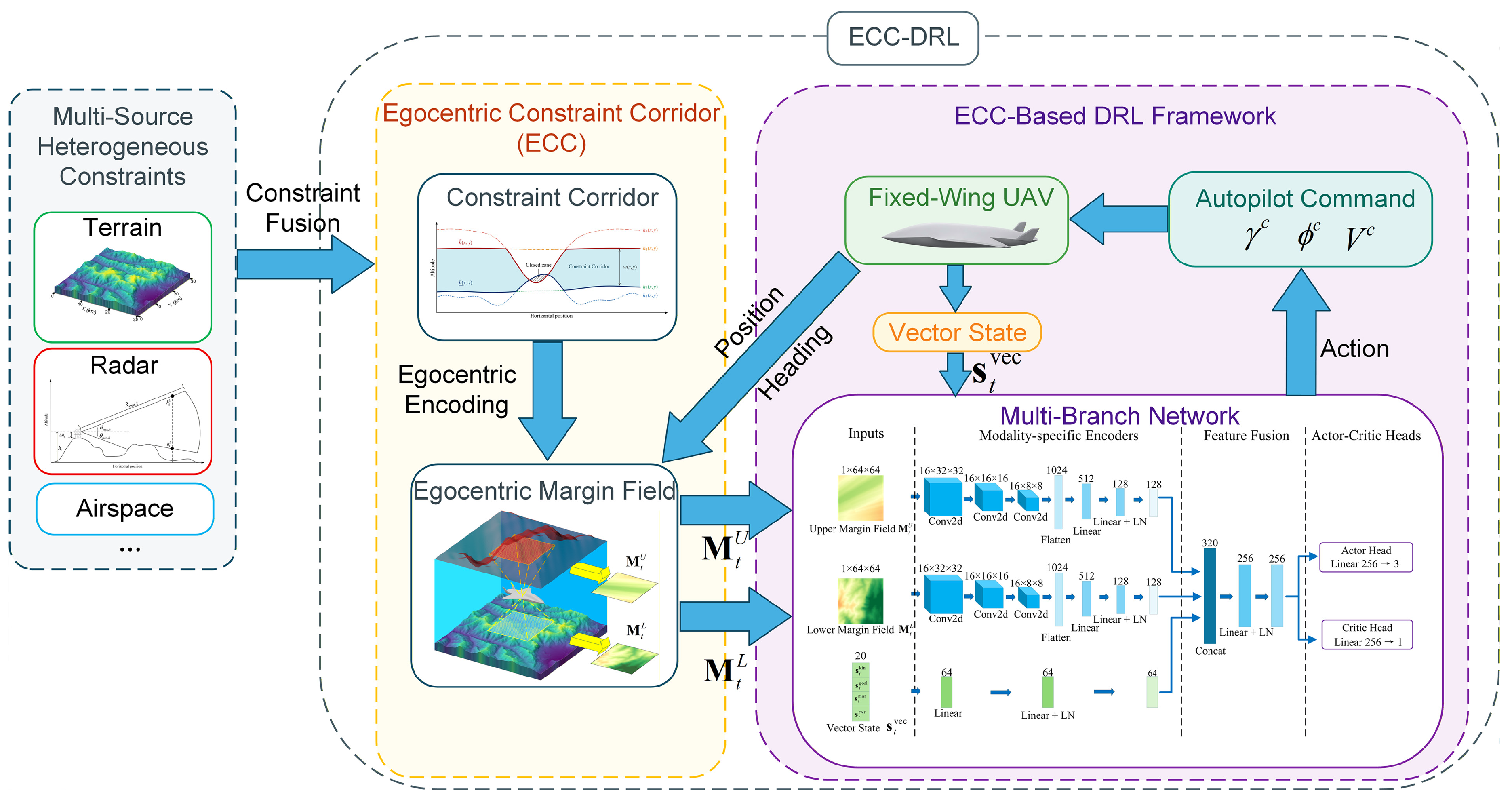
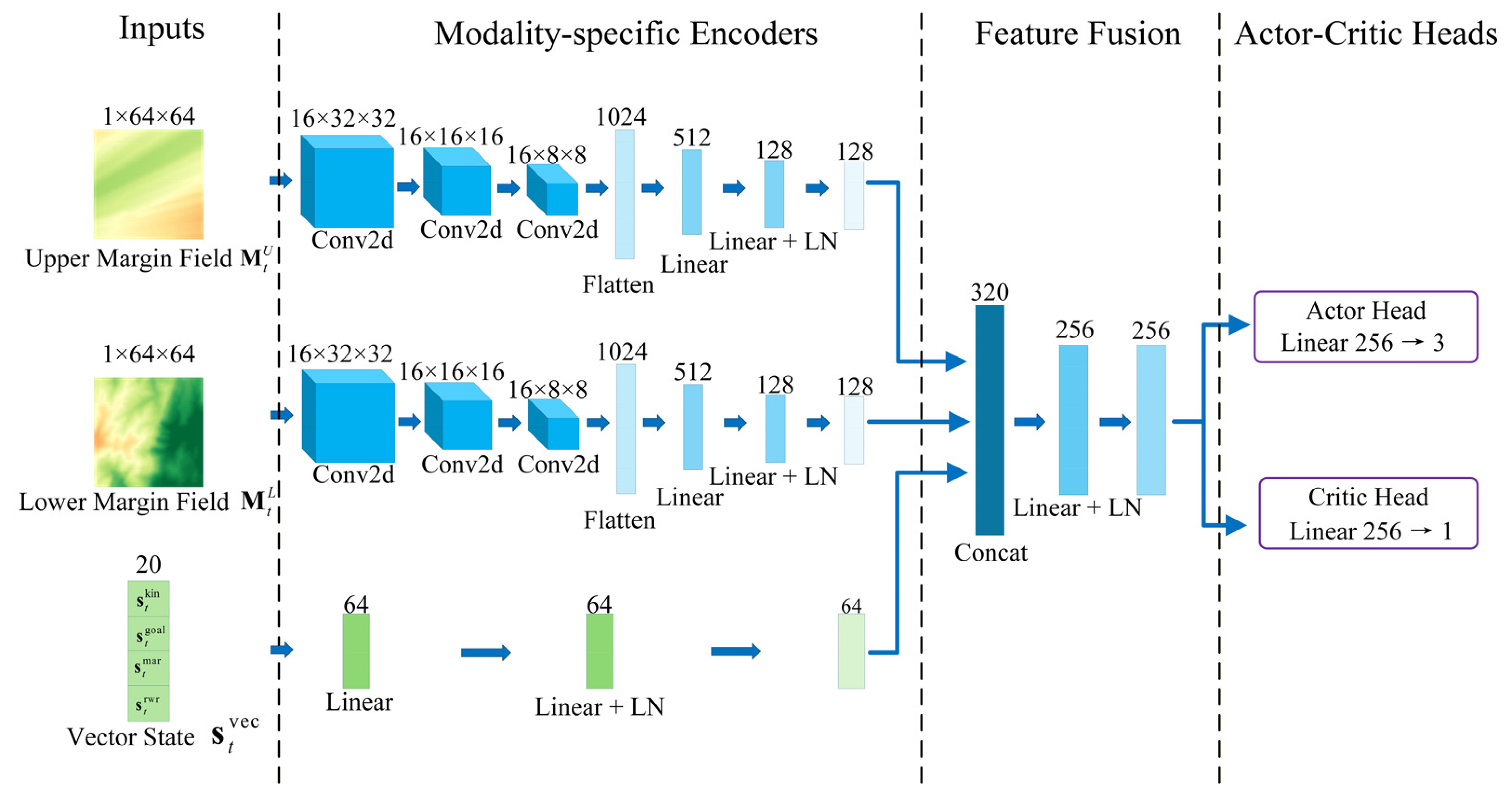
This paper proposes the Egocentric Constraint Corridor (ECC), a constraint representation method that converts heterogeneous multi-source constraints into structured observations directly usable by a navigation policy, and builds a deep reinforcement learning navigation framework upon ECC. ECC performs constraint fusion and egocentric encoding upstream of the policy. Specifically, ECC is constructed in two steps: first, heterogeneous multi-source constraints are fused into upper and lower boundary surfaces to define the constraint corridor; then, the surrounding corridor is egocentrically encoded relative to the vehicle’s current position to produce an egocentric margin field, which provides the policy with spatial constraint information around the vehicle as observation input. On this basis, a multi-branch network is designed to separately extract and fuse features from the egocentric margin field and vector state, and a composite reward function is employed to balance constraint satisfaction with navigation efficiency. The corridor navigation policy is obtained through end-to-end reinforcement learning training. The complete navigation method based on ECC is denoted ECC-DRL. Figure 1 presents the overall framework of ECC-DRL.

Figure 1. Overall framework of ECC-DRL. Heterogeneous multi-source constraints are fused and egocentrically encoded to produce the egocentric margin field, which, together with the vector state, is fed into a multi-branch network that outputs autopilot commands to the vehicle; the vehicle’s kinematic state feeds back into the egocentric encoding and vector state construction, forming a closed-loop navigation system.

The main contributions of this paper are as follows:

• Egocentric Constraint Corridor. Heterogeneous multi-source constraints are fused into upper and lower boundary surfaces to define a constraint corridor, which is then encoded as a normalized vertical margin field centered on the vehicle. This margin field captures the relative geometry between the vehicle and the surrounding corridor, causing geometrically similar corridor segments to produce consistent observations and thereby providing a foundation for cross-scenario policy transfer;
• ECC-based deep reinforcement learning navigation framework. A multi-branch network and a composite reward function are designed around the structure of ECC: the two margin field channels are encoded by independent convolutional branches because the upper and lower boundaries are governed by constraint sources of different spatial character, and the reward function distinguishes hard from soft constraints according to the recoverability of the fused constraint sources. The framework achieves three-dimensional autonomous navigation within vertically constrained corridors;
• Systematic experimental validation. Comparative experiments against A* and Dubins-RRT* demonstrate the online decision efficiency advantage of ECC-DRL. Ablation studies confirm that the egocentric margin field is a necessary condition for reliable corridor navigation. Zero-shot cross-scenario transfer validates the generalization capability of egocentric encoding, and hardware-in-the-loop experiments on an embedded platform verify the feasibility of real-time closed-loop operation under resource constraints.

The remainder of this paper is organized as follows. Section 2 reviews related work. Section 3 establishes the UAV kinematic model and constraint models for terrain, airspace, and radar detection. Section 4 defines the Egocentric Constraint Corridor, including the geometric construction of the constraint corridor and the egocentric encoding method. Section 5 builds the deep reinforcement learning navigation framework on the ECC representation. Section 6 presents comparative, ablation, transfer, and hardware-in-the-loop experiments with analysis. Section 7 discusses the results, limitations, and future work. Section 8 concludes the paper.

2. Related Work

2.1. UAV Path Planning

UAV path planning aims to find a trajectory from a start point to a goal in a three-dimensional constrained environment that satisfies safety and kinematic requirements. Existing methods mainly fall into graph search, sampling-based, and optimization paradigms.

Graph search methods discretize the flight space into grids or graphs and search for cost-optimal trajectories. In three-dimensional UAV path planning, the A* algorithm has been widely adopted and improved owing to its optimality under consistent heuristics: Qi et al. introduced virtual terrain on digital maps to compress the search space and then generated three-dimensional trajectories with an improved heuristic A* [13]; Zhang et al. addressed the limitations of grid resolution and heuristic design by proposing a direction-aware adaptive heuristic to improve planning efficiency and success rate in complex scenarios [14]; Pelosi et al. searched for constrained fixed-wing UAV trajectories on grids that fuse terrain and detection costs using A* [15]. However, the computational and memory costs of these methods grow with grid scale, which is particularly pronounced in large-scale or cluttered environments, and the resulting piecewise-linear trajectories typically require additional smoothing to satisfy kinematic constraints.

Sampling-based methods incrementally construct feasible trajectories through random sampling in the configuration space and are well suited for high-dimensional planning problems. Rapidly-exploring random trees and their asymptotically optimal variants have been widely used in three-dimensional UAV path planning. To address the low sampling efficiency in narrow passages, Huang et al. introduced adaptive bidirectional sampling and cost redefinition to improve convergence speed and success rate in narrow corridors [16]; Lim et al. tackled the problem that fixed-wing aircraft in steep terrain may enter inevitable-collision states due to altitude constraints by efficiently identifying such states via periodic paths and generating kinematically feasible safe trajectories with a sampling-based planner [17]. However, the inherent randomness of sampling leads to unstable planning results without guarantees on trajectory quality, and finding feasible solutions becomes particularly difficult in segments where the feasible space is narrow.

Optimization methods formulate trajectory generation as constrained optimization problems. Model predictive control repeatedly solves optimization problems over a receding horizon to generate UAV trajectories that satisfy dynamic and collision-avoidance constraints [18]. In addition, metaheuristic methods such as particle swarm optimization and genetic algorithms search for near-optimal trajectories under complex constraints through population-based stochastic search and have been widely applied to UAV path planning [19]. Liu et al. proposed the safe flight corridor method, which decomposes free space into a sequence of convex polyhedra to construct a convex feasible region, enabling efficient trajectory optimization for quadrotors under convex constraints [20]; Zhong et al. further generated convex polyhedra directly on onboard point clouds to reduce computational overhead [21]. Optimization methods can explicitly handle constraints but incur substantial online computational costs and rely on relatively accurate environmental and dynamic models.

Overall, the above path planning methods can yield high-quality or even optimal trajectories when complete environmental information is available; however, their online computational cost grows with the scale and constraint complexity of the environment, limiting the real-time applicability of a single planning run in large-scale or complex scenarios.

2.2. Deep Reinforcement Learning for UAV Navigation

Deep reinforcement learning can generate online decisions from local observations, offering a new avenue for the computational cost and re-computation problems described above, and has been widely applied to UAV autonomous navigation and obstacle avoidance in recent years. Existing work primarily targets environments containing obstacles and investigates how to achieve safe navigation based on onboard perception information. Camci et al. used forward-facing depth images as input to generate motion primitives end-to-end, guiding quadrotors through cluttered environments [22]; He et al. introduced expert demonstrations on top of TD3 to accelerate training, likewise using depth images as observations for navigation in unknown three-dimensional environments [23]. Fan et al. compressed multi-frame LiDAR point clouds into two-dimensional obstacle maps to achieve end-to-end obstacle avoidance in dynamic environments [24]. For fixed-wing platforms, Wu et al. used gridded obstacle distributions within the field of view as input for reactive obstacle avoidance [25], and Su et al. achieved lightweight obstacle avoidance under fixed-wing dynamic constraints using single-frame monocular depth estimation as the observation [26]. These studies differ primarily in the sensing modality from which the observation is constructed.

Beyond the choice of sensing modality, the construction of the observation has itself been treated as a design problem in its own right, one that bears on policy performance and cross-environment generalization independently of the policy optimization algorithm. Sheng et al. analyzed how the position and attitude changes of a vehicle affect navigation performance in complex environments and proposed a state space representation incorporating both [27]; Fahmy et al. organized the observation as multichannel cost maps carrying spatial and temporal information, and reported markedly faster convergence and higher navigation efficiency in narrow passages than observations built from raw sensor data or stacked frames [28]. Other work acts on the dimensionality and spatial scale of the observation: Xu et al. compressed raw perception into a compact low-dimensional input [29], and Han et al. employed multi-scale state representations to balance coverage against dimensionality, demonstrating cross-environment policy transferability [30]. Wang et al. instead addressed the information available during training, introducing privileged information to mitigate observation degradation under partial observability [31]. Still other work assembles content of different kinds into a single observation: Jun et al. fused static obstacles with dynamic risk zones into one occupancy map serving as the policy state and encoded it into sector-wise relative spatial features [32], and Mari et al. combined goal-related quantities, a virtual occupancy grid and boundary ray-casting into a single observation vector [33].

Across all of the above work, however the observation is organized, the quantity it encodes is the occupancy of obstacles or of free space, and it is obtained, directly or after processing, from the vehicle’s perception of its surroundings. Corridor navigation calls for a different quantity: the vertical margin from the vehicle to constraint surfaces jointly defined by terrain elevation, detection envelopes and airspace regulations. These sources differ in physical nature and data modality; none of them is directly readable by an onboard sensor, and their fusion must therefore be performed upstream of the policy rather than obtained from perception. Existing observation designs therefore offer no unified representation of these constraints: the difference lies not in the form of the observation but in the quantity it encodes and in where that quantity is obtained.

3. System Model

3.1. UAV Kinematic Model

The UAV is modeled as a three-degree-of-freedom point mass. In the north–east–down (NED) inertial frame, the velocity vector of the UAV can be expressed in terms of the airspeed $V$, course angle $\chi$, and flight-path angle $\gamma$ as [34]

$$\mathbf{v}=V\left(\begin{array}{c}\cos \chi \cos \gamma \\ \sin \chi \cos \gamma \\ -\sin \gamma \end{array}\right).$$

(1)

Denoting the horizontal position by $\left(x, y\right)$ and the altitude by $h$, the kinematic equations are:

$$\left(\begin{array}{c}\dot{x}\\ \dot{y}\\ \dot{h}\end{array}\right)=V\left(\begin{array}{c}\cos \chi \cos \gamma \\ \sin \chi \cos \gamma \\ \sin \gamma \end{array}\right).$$

(2)

This paper assumes a no-wind environment, so that the course angle $\chi$ equals the heading angle $\psi$ and the ground speed equals the airspeed.

Under the coordinated-turn condition with zero sideslip, the rate of change of the course angle is given by the bank angle $\varphi$:

$$\dot{\chi }={\displaystyle \frac{g}{V}}\tan \varphi .$$

(3)

A low-level autopilot is assumed to regulate the airspeed $V$, flight-path angle $\gamma$, and bank angle $\varphi$ toward their respective commanded values $V^c$, ${\gamma }^c$, and ${\varphi }^c$. The closed-loop response of each autopilot channel is approximated as a first-order system:

$$\dot{\varphi }=b_{\varphi }\left({\varphi }^c-\varphi \right),$$

(4a)

$$\dot{\gamma }=b_{\gamma }\left({\gamma }^c-\gamma \right),$$

(4b)

$$\dot{V}=b_V\left(V^c-V\right),$$

(4c)

where $b_{\varphi }$, $b_{\gamma }$, and $b_V$ are positive constants. The state variables are bounded by $\left|\varphi \right|\le {\varphi }_{\mathrm{m}\mathrm{a}\mathrm{x}}$, $\left|\gamma \right|\le {\gamma }_{\mathrm{m}\mathrm{a}\mathrm{x}}$, and $V_{\mathrm{m}\mathrm{i}\mathrm{n}}\le V\le V_{\mathrm{m}\mathrm{a}\mathrm{x}}$. The response rates of the channels in Equation (4) are further limited by $\left|\dot{\varphi }\right|\le {\dot{\varphi }}_{\mathrm{m}\mathrm{a}\mathrm{x}}$, $\left|\dot{\gamma }\right|\le {\dot{\gamma }}_{\mathrm{m}\mathrm{a}\mathrm{x}}$, and $\left|\dot{V}\right|\le a_{\mathrm{m}\mathrm{a}\mathrm{x}}$.

3.2. Terrain and Airspace Model

Terrain elevation is provided by a digital elevation model and represented as a continuous function $h_{\mathrm{T}}\left(x,y\right):{\mathbb{R}}^2\to \mathbb{R}$ that returns the ground elevation at horizontal position $\left(x,y\right)$. The terrain surface is defined as:

$$z=h_{\mathrm{T}}\left(x,y\right).$$

(5)

The airspace altitude ceiling is represented as a continuous function $h_{\mathrm{A}}\left(x,y\right):{\mathbb{R}}^2\to \mathbb{R}$, denoting the maximum permissible flight altitude at that position. The airspace ceiling surface is defined as

$$z=h_{\mathrm{A}}\left(x,y\right).$$

(6)

Both terrain and airspace constraints are assumed to be time-invariant during the mission. The flight altitude of the UAV must satisfy:

$$h_{\mathrm{T}}\left(x\left(t\right),y\left(t\right)\right)+{\delta }_{\mathrm{m}\mathrm{i}\mathrm{n}}\le h\left(t\right)\le h_{\mathrm{A}}\left(x\left(t\right),y\left(t\right)\right),$$

(7)

where ${\delta }_{\mathrm{m}\mathrm{i}\mathrm{n}}$ is the minimum safety clearance above the ground.

3.3. Radar Detection Model

Each ground-based radar $k$ is characterized by its horizontal position $\left(x_k{,y}_k\right)$, antenna height above ground $\Delta h_k$, maximum detection slant range $R_{\mathrm{m}\mathrm{a}\mathrm{x},k}$, maximum elevation angle ${\theta }_{\mathrm{m}\mathrm{a}\mathrm{x},k}$, and minimum elevation angle ${\theta }_{\mathrm{m}\mathrm{i}\mathrm{n},k}$. The absolute elevation of the antenna of radar $k$ is

$$h_k=h_{\mathrm{T}}\left(x_k,y_k\right)+\Delta h_k.$$

(8)

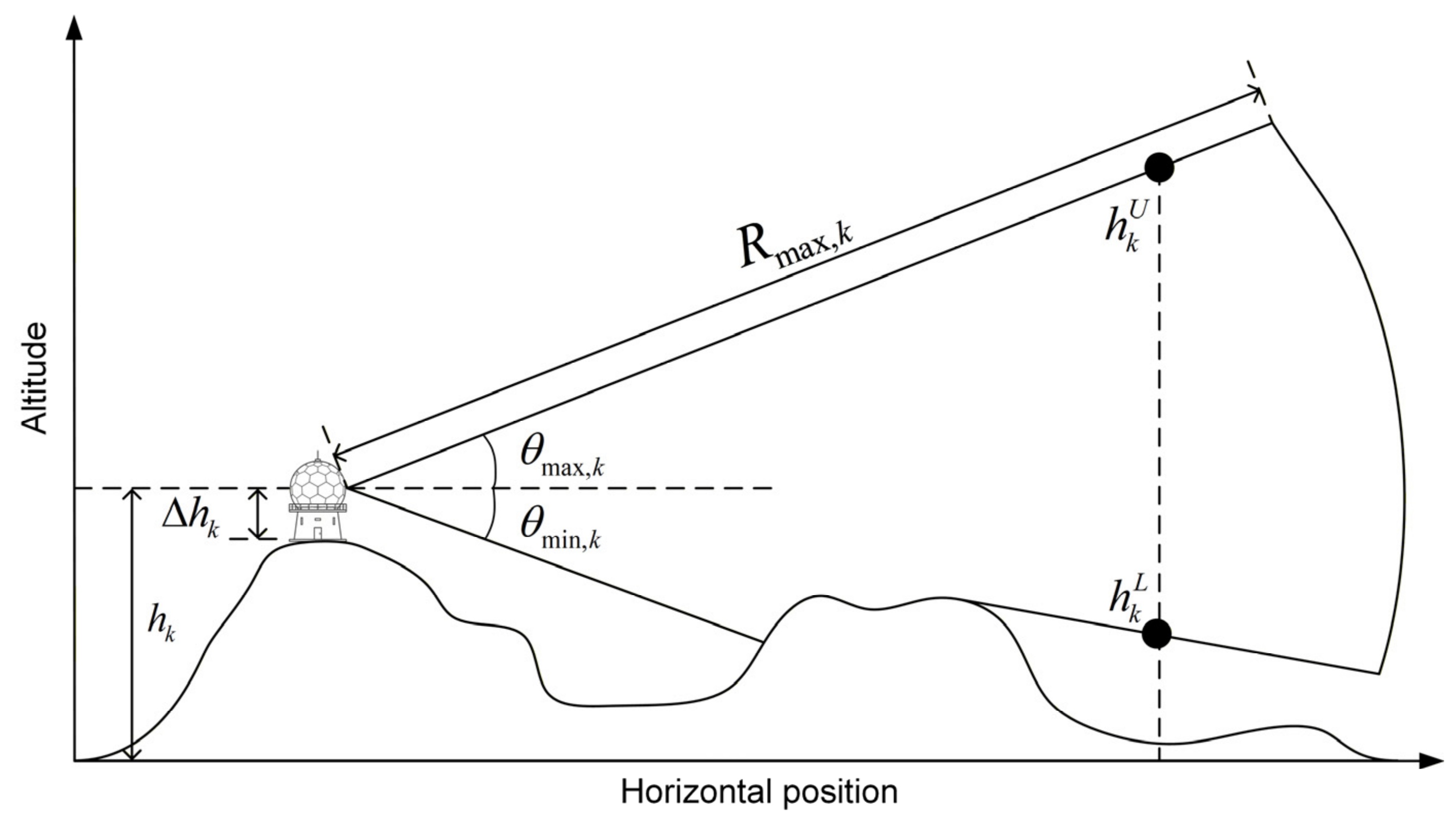
The geometry of the detection envelope of a single radar is illustrated in Figure 2. The detectable altitude range at each horizontal position $\left(x,y\right)$ is bounded by the upper detection altitude $h_k^U\left(x,y\right)$ and the lower detection altitude $h_k^L\left(x,y\right)$. Terrain undulations can mask radar electromagnetic propagation, creating low-altitude detection blind zones behind ridgelines.

Figure 2. Horizontal-range–altitude profile of a single radar detection envelope. $h_k^U$ and $h_k^L$ denote the upper and lower detection altitudes, respectively; terrain masking of the radar line of sight raises the lower detection boundary.

3.3.1. Radar Detection Envelope

Let $d_k=‖\left(x-x_k,\hspace{0.25em}y-y_k\right)‖$ denote the horizontal distance from an arbitrary position $\left(x,y\right)$ to radar $k$.

For the region where $d_k\le R_{\max ,k}$, the upper detection altitude is the lower of the cone corresponding to the maximum elevation angle and the sphere corresponding to the maximum slant range:

$$h_k^U\left(x,y\right)=\min \left(h_k+d_k\mathrm{t}\mathrm{a}\mathrm{n}{\theta }_{\mathrm{m}\mathrm{a}\mathrm{x},k}, h_k+\sqrt{R_{\mathrm{m}\mathrm{a}\mathrm{x},k}^2-d_k^2}\right)+c\left(d_k\right),$$

(9)

where $c\left(d_k\right)={\displaystyle \frac{d_k^2}{\left(2R_e\right)}}$ is the Earth curvature correction and $R_e={\displaystyle \frac{4}{3}}{R}_{\oplus }$ is the effective Earth radius under standard atmospheric refraction [35].

The lower detection altitude is the maximum of four terms—ground elevation, terrain masking, minimum elevation angle, and slant-range lower bound:

$$h_k^L\left(x,y\right)=\max \left(h_{\mathrm{T}}\left(x,y\right), h_k^{\mathrm{mask}}, h_k^{\mathrm{cone}}, h_k^{\mathrm{sphere}}\right),$$

(10)

where $h_{\mathrm{T}}\left(x,y\right)$ is the ground elevation, ensuring the lower detection boundary does not fall below the terrain; $h_k^{\mathrm{mask}}$, $h_k^{\mathrm{cone}}$, and $h_k^{\mathrm{sphere}}$ are the terrain-masking component, the minimum-elevation-angle component, and the slant-range lower-bound component, defined by Equations (11)–(14).

The terrain-masking component reflects the elevation of the line of sight caused by ridges between the radar and the target:

$$h_k^{\mathrm{mask}}\left(x,y\right)=h_k+d_k\mathrm{t}\mathrm{a}\mathrm{n}{\alpha }_k\left(x,y\right)+c\left(d_k\right),$$

(11)

where ${\alpha }_k\left(x,y\right)$ is the maximum masking elevation angle along the terrain profile from the radar to the target:

$${\alpha }_k\left(x,y\right)=\underset{\left(x^{\prime },y^{\prime }\right)\in \mathcal{L}\left(k\to \left(x,y\right)\right)}{\mathrm{m}\mathrm{a}\mathrm{x}}\mathrm{a}\mathrm{r}\mathrm{c}\mathrm{t}\mathrm{a}\mathrm{n}{\displaystyle \frac{h_{\mathrm{T}}\left(x^{\prime },y^{\prime }\right)-h_k-c\left(d^{\prime }\right)}{d^{\prime }}},$$

(12)

where $\mathcal{L}\left(k\to \left(x,y\right)\right)$ is the set of intermediate sample points along the horizontal line from the radar to the target, excluding the target point itself, and $d^{\prime }$ is the horizontal distance from each sample point to the radar.

The minimum-elevation-angle component corresponds to the cone defined by the beam elevation lower limit:

$$h_k^{\mathrm{cone}}\left(x,y\right)=h_k+d_k\mathrm{t}\mathrm{a}\mathrm{n}{\theta }_{\mathrm{m}\mathrm{i}\mathrm{n},k}+c\left(d_k\right).$$

(13)

The slant-range lower-bound component corresponds to the lower hemisphere of the sphere defined by the maximum detection slant range, causing the detection envelope to close vertically as $d_k\to R_{\mathrm{m}\mathrm{a}\mathrm{x},k}$:

$$h_k^{\mathrm{sphere}}\left(x,y\right)=h_k-\sqrt{R_{\mathrm{m}\mathrm{a}\mathrm{x},k}^2-d_k^2}+c\left(d_k\right).$$

(14)

All radars are assumed to operate independently, and a target at $\left(x,y,z\right)$ is considered detected if it lies within the detection interval of at least one radar covering $\left(x,y\right)$. The detected altitude set at $\left(x,y\right)$ is therefore the union of the individual detection intervals, $\mathcal{D}\left(x,y\right)={\bigcup }_{k: d_k\le R_{\max ,k}}\left[h_k^L\left(x,y\right), h_k^U\left(x,y\right)\right]$, which may be disconnected. To provide a single interface for the geometric partition of the corridor, the upper and lower detection altitudes of the fused multi-radar detection envelope are constructed as a single interval by taking the minimum of the lower detection altitudes and the maximum of the upper detection altitudes over the radars covering each horizontal position:

$$h^U\left(x,y\right)=\underset{k: d_k\le R_{\mathrm{m}\mathrm{a}\mathrm{x},k}}{\mathrm{m}\mathrm{a}\mathrm{x}}{h}_k^U\left(x,y\right),$$

(15)

$$h^L\left(x,y\right)=\underset{k: d_k\le R_{\mathrm{m}\mathrm{a}\mathrm{x},k}}{\mathrm{m}\mathrm{i}\mathrm{n}}{h}_k^L\left(x,y\right).$$

(16)

so that $\mathcal{D}\left(x,y\right)\subseteq \left[h^L\left(x,y\right),h^U\left(x,y\right)\right]$. When the detection intervals of two radars are disjoint in altitude, this construction includes the altitude band between them in the constrained region, and Equations (15) and (16) therefore constitute an outer approximation of the union. This approximation is adopted for two reasons. First, the approximation only enlarges the constrained region, and every detected altitude is contained within it, so the error is on the conservative side. Second, such an altitude band is immediately adjacent to the detection intervals above and below it and leaves no vertical margin; therefore, it remains a high-risk region in the presence of radar parameter and altitude tracking errors.

If a horizontal position is not within the detection range of any radar, no radar detection constraint exists at that position.

$$z=h^U\left(x,y\right),$$

(17)

$$z=h^L\left(x,y\right).$$

(18)

3.3.2. Detection Intensity and Warning Signal

The detection intensity of radar $k$ toward a target located at $\left(x,y,z\right)$ is defined using a parametric approximation [15] based on the inverse fourth-power range law of the radar equation [35]:

$$S_k=\left\{\begin{array}{ll}{\displaystyle \frac{\eta }{\eta +{\left(\frac{r_k}{R_{\mathrm{m}\mathrm{a}\mathrm{x},k}}\right)}^4}},& h_k^L\le z\le h_k^U \mathrm{and} d_k\le R_{\mathrm{m}\mathrm{a}\mathrm{x},k}\\ 0,& \mathrm{otherwise}\end{array}\right.,$$

(19)

where $r_k=‖\left(x-x_k,\hspace{0.33em}y-y_k,\hspace{0.33em}z-h_k\right)‖$ is the slant range from the target to the radar and $\eta >0$ is a shape parameter controlling the decay rate of the detection intensity with distance. $S_k$ takes values in $[0,1]$, decreases monotonically with slant range, and is zero outside the detection envelope; it is used as the equivalent detection probability of radar $k$ in the subsequent evaluation.

The UAV is equipped with a radar warning receiver (RWR) that aggregates detection intensity into $N_s$ equal angular sectors relative to the current course angle $\chi$:

$$\mathrm{R}\mathrm{W}\mathrm{R}\left(j\right)=\underset{k\in {\mathcal{K}}_j}{\mathrm{m}\mathrm{a}\mathrm{x}}{S}_k, j=1,\dots ,N_s,$$

(20)

where ${\mathcal{K}}_j$ is the set of radars whose relative bearings fall within the j-th sector, and $N_s$ is the total number of sectors. This sectored aggregation provides the navigation policy with bearing-resolved threat information.

4. Egocentric Constraint Corridor

4.1. Constraint Corridor

In the constrained airspace, the flight altitude of the UAV at each horizontal position is restricted by multiple constraint sources. Each constraint source defines a constraint surface that imposes a one-sided bound on the flight altitude. Denoting the altitude function of each constraint surface as $h_i\left(x,y\right)$, these are classified into two categories by constraint direction: lower-boundary constraint surfaces require the UAV to fly above them, i.e., $h\ge h_i\left(x,y\right)$; upper-boundary constraint surfaces require the UAV to fly below them, i.e., $h\le h_i\left(x,y\right)$. Some constraint sources define altitude intervals to be avoided rather than one-sided bounds. For such sources, the vehicle must be pre-assigned to pass above or below the avoidance interval according to mission requirements, converting it into a one-sided constraint surface before inclusion in the above classification.

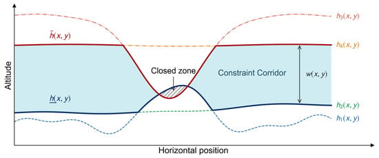
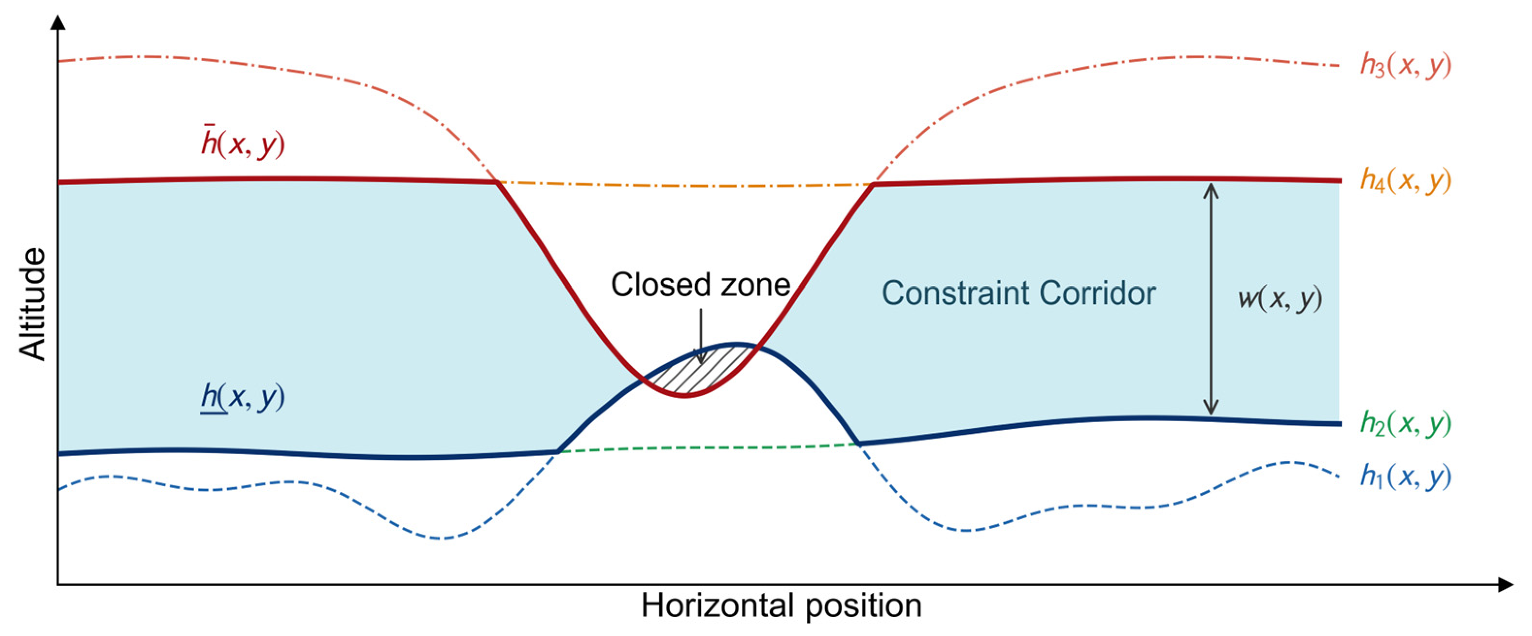
Since the constraint corridor at each horizontal position is a vertical altitude interval, its geometry is fully determined by the two endpoints of the interval. The altitude of the corridor’s lower boundary surface is the maximum of all lower-boundary constraint surfaces at that position, and the altitude of the upper boundary surface is the minimum of all upper-boundary constraint surfaces:

$$\underset{\_}{h}\left(x,y\right)=\underset{i: \mathrm{l}\mathrm{o}\mathrm{w}\mathrm{e}\mathrm{r}}{\mathrm{m}\mathrm{a}\mathrm{x}}{h}_i\left(x,y\right),$$

(21)

$$\overline{h}\left(x,y\right)=\underset{i: \mathrm{u}\mathrm{p}\mathrm{p}\mathrm{e}\mathrm{r}}{\mathrm{m}\mathrm{i}\mathrm{n}}{h}_i\left(x,y\right),$$

(22)

where $\underset{\_}{h}\left(x,y\right)$ and $\overline{h}\left(x,y\right)$ are the altitude functions of the lower and upper boundary surfaces of the constraint corridor, respectively. The lower and upper boundary surfaces are defined as

$$z=\underset{\_}{h}\left(x,y\right),$$

(23)

$$z=\overline{h}\left(x,y\right).$$

(24)

The constraint corridor is defined as the three-dimensional spatial region between the upper and lower boundary surfaces:

$$\mathcal{C}=\{\left(x,y,z\right)\hspace{0.33em}\left|\hspace{0.33em}\underset{\_}{h}\left(x,y\right)\le z\le \overline{h}\left(x,y\right)\right\}.$$

(25)

The vertical thickness of the constraint corridor at position $\left(x,y\right)$ is

$$w\left(x,y\right)=\overline{h}\left(x,y\right)-\underset{\_}{h}\left(x,y\right).$$

(26)

When $w\left(x,y\right)\le 0$, the upper and lower boundary surfaces intersect or coincide, and the constraint corridor closes at that position. Figure 3 illustrates a vertical cross-section of the constraint corridor.

Figure 3. Vertical cross-section of the constraint corridor. Individual constraint surfaces are shown as dashed lines; their fusion yields the corridor’s upper and lower boundary surfaces, shown as solid lines. The lightly shaded region is the constraint corridor, the hatched region marks closed segments, and $w\left(x,y\right)$ denotes the vertical thickness of the corridor.

4.2. Egocentric Margin Field

Section 4.1 defined the geometry of the constraint corridor in the global coordinate frame. However, what the navigation policy needs to perceive is the relative geometry between the vehicle and the surrounding corridor—specifically, how much vertical clearance remains in each direction from the vehicle’s current position and altitude to the upper and lower boundary surfaces. To this end, this section encodes the constraint corridor as an egocentric margin field.

At a horizontal position $\left(x,y\right)$, taking the UAV’s current altitude $h_0$ as the reference, the upper margin and lower margin are defined as

$$m^U\left(x,y\right)=\overline{h}\left(x,y\right)-h_0,$$

(27)

$$m^L\left(x,y\right)=h_0-\underset{\_}{h}\left(x,y\right).$$

(28)

$m^U$ represents the vertical clearance from the current altitude to the upper boundary surface at that horizontal position, and $m^L$ represents the clearance to the lower boundary surface. When both are positive, the UAV is inside the constraint corridor; a negative value of either indicates that the current altitude has exceeded the corresponding boundary at that position; in closed corridor segments, both are simultaneously negative.

To organize the margin information of the surrounding corridor into a spatially structured observation, an egocentric coordinate frame $\left(\xi ,\zeta \right)$ is established with the UAV’s current horizontal position $\left(x_0,y_0\right)$ as the origin and the current course angle ${\chi }_0$ as the forward axis:

$$\left(\begin{array}{c}\xi \\ \zeta \end{array}\right)=\left(\begin{array}{cc}\mathrm{c}\mathrm{o}\mathrm{s}{\chi }_0& \mathrm{s}\mathrm{i}\mathrm{n}{\chi }_0\\ -\mathrm{s}\mathrm{i}\mathrm{n}{\chi }_0& \mathrm{c}\mathrm{o}\mathrm{s}{\chi }_0\end{array}\right)\left(\begin{array}{c}x-x_0\\ y-y_0\end{array}\right),$$

(29)

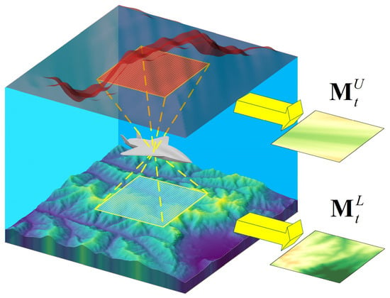
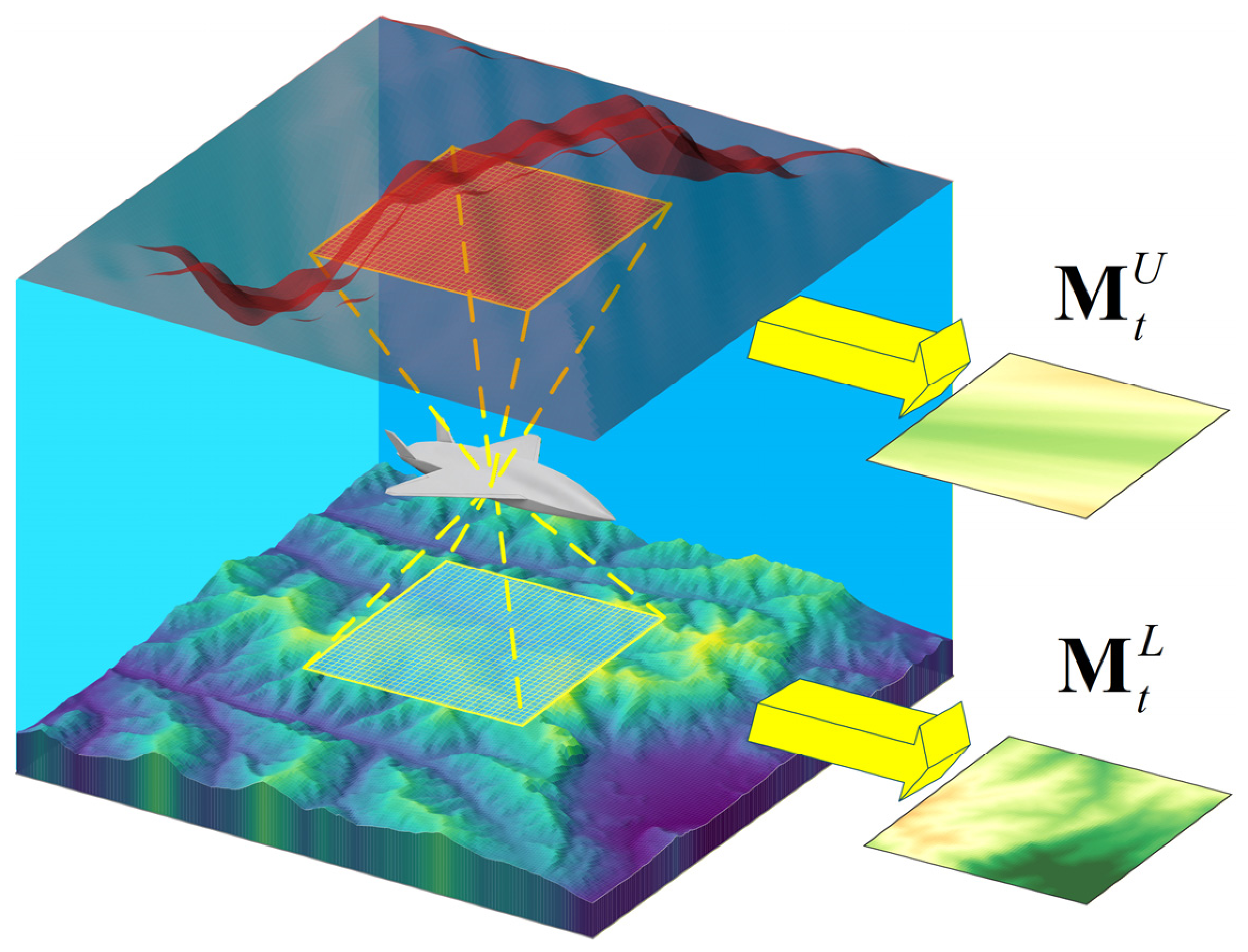
where $\xi$ is aligned with the forward direction and $\zeta$ with the lateral direction. As illustrated in Figure 4, a rectangular sampling grid of size $N_{\xi }\times N_{\zeta }$ is established in the egocentric frame, with grid points $\left\{\left({\xi }_p,{\zeta }_q\right)\right\}$, $p=1,\dots ,N_{\xi }$, $q=1,\dots ,N_{\zeta }$, centered at the origin and symmetrically distributed along both the $\xi$ and $\zeta$ axes. The grid is thus fixed to the vehicle and centered on it, following the construction of robocentric local maps in mobile robot and aerial navigation [36]; since the frame rotates with the course angle, a change of heading rotates the sampled neighborhood about the vehicle, keeping the surrounding corridor covered in all directions. Each grid point is mapped back to global coordinates $\left(x_{pq},y_{pq}\right)$ via the inverse of Equation (29), and margin values are computed by Equations (27) and (28) and normalized by a reference height $h_{\mathrm{r}\mathrm{e}\mathrm{f}}$ to form the upper and lower margin fields:

$${\mathbf{M}}^U\in {\mathbb{R}}^{N_{\xi }\times N_{\zeta }}, M_{pq}^U={\displaystyle \frac{\overline{h}\left(x_{pq}, y_{pq}\right)-h_0}{h_{\mathrm{r}\mathrm{e}\mathrm{f}}}},$$

(30)

$${\mathbf{M}}^L\in {\mathbb{R}}^{N_{\xi }\times N_{\zeta }}, M_{pq}^L={\displaystyle \frac{h_0-\underset{\_}{h}\left(x_{pq}, y_{pq}\right)}{h_{\mathrm{r}\mathrm{e}\mathrm{f}}}}.$$

(31)

Figure 4. Construction of the egocentric margin field. The vehicle establishes a sampling grid centered on its current position along the forward and lateral directions, projects each grid point onto the upper and lower boundary surfaces, and computes the normalized vertical margin at each point, forming the upper margin field ${\mathbf{M}}_t^U$ and the lower margin field ${\mathbf{M}}_t^L$.

${\mathbf{M}}^U$ and ${\mathbf{M}}^L$ constitute the spatial observation input of the navigation policy, encoding the normalized vertical clearance from the vehicle to the upper and lower boundary surfaces in all surrounding directions. Each is a two-dimensional grid of size $N_{\xi }\times N_{\zeta }$ whose structure resembles a single-channel image and can be processed directly by a convolutional network. The coordinate transformation in Equation (29) together with the normalized sampling in Equations (30) and (31) are collectively referred to as egocentric encoding. The key property of egocentric encoding is as follows: the translation in Equation (29) sets the vehicle’s position as the origin, eliminating the margin field’s dependence on the global position; the rotation aligns the course angle with the forward axis, eliminating the dependence on the absolute heading. Consequently, geometrically similar constraint corridors produce consistent margin fields regardless of where they appear on the map or from which direction the vehicle approaches. Normalization further removes the influence of absolute scale. These properties ensure that the policy’s input depends only on the relative geometry between the vehicle and the surrounding constraint corridor, providing the foundation for zero-shot cross-scenario policy transfer.

5. ECC-Based Deep Reinforcement Learning Navigation Framework

5.1. MDP Formulation

The corridor navigation task is formulated as a Markov decision process $\left(\mathcal{S},\mathcal{A},\mathcal{T},R,{\gamma }_d\right)$, where $\mathcal{S}$ is the state space, $\mathcal{A}$ is the action space, $\mathcal{T}$ is the state transition function defined by the kinematic model in Section 3.1, $R$ is the reward function, and ${\gamma }_d$ is the discount factor.

State Space. The state consists of the margin field and a vector state:

$$s_t=\left({\mathbf{M}}_t,\hspace{0.33em}{\mathbf{s}}_t^{\mathrm{v}\mathrm{e}\mathrm{c}}\right).$$

(32)

Here ${\mathbf{M}}_t$ denotes the upper and lower margin fields and ${\mathbf{s}}_t^{\mathrm{v}\mathrm{e}\mathrm{c}}\in {\mathbb{R}}^{n_s}$ denotes the vector state. ${\mathbf{M}}_t$ comprises the upper margin field ${\mathbf{M}}_t^U$ and the lower margin field ${\mathbf{M}}_t^L$ (Equations (30) and (31)):

$${\mathbf{M}}_t=\left({\mathbf{M}}_t^U,\hspace{0.33em}{\mathbf{M}}_t^L\right), {\mathbf{M}}_t^U, {\mathbf{M}}_t^L\in {\mathbb{R}}^{N_{\xi }\times N_{\zeta }}.$$

(33)

In this paper, the upper margin field ${\mathbf{M}}_t^U$ is determined by the airspace ceiling surface (Equation (6)) and the fused multi-radar lower detection boundary surface (Equation (18)), while the lower margin field ${\mathbf{M}}_t^L$ is determined by the terrain surface (Equation (5)). Among these three boundary surfaces, the terrain surface and the airspace ceiling surface are hard constraints: crossing either is irrecoverable, as the vehicle is lost in the first case and the mission is void in the second. The fused multi-radar lower detection boundary is a soft constraint: after penetration, the vehicle remains airworthy and can continue toward the goal, accumulating detection exposure that grows with the depth and duration of the penetration. The values of both margin fields are clipped to $\left[-1,1\right]$; grid points outside the mission region $\mathcal{R}$ are assigned a fixed value of 2.0, outside the clipping range, to indicate the boundary.

The vector state is the concatenation of four components:

$${\mathbf{s}}_t^{\mathrm{v}\mathrm{e}\mathrm{c}}=[{\mathbf{s}}_t^{\mathrm{k}\mathrm{i}\mathrm{n}},\hspace{0.33em}\hspace{0.33em}{\mathbf{s}}_t^{\mathrm{g}\mathrm{o}\mathrm{a}\mathrm{l}},\hspace{0.33em}\hspace{0.33em}{\mathbf{s}}_t^{\mathrm{m}\mathrm{a}\mathrm{r}},\hspace{0.33em}\hspace{0.33em}{\mathbf{s}}_t^{\mathrm{r}\mathrm{w}\mathrm{r}}{]}^{\mathrm{\top }}.$$

(34)

The kinematic state ${\mathbf{s}}_t^{\mathrm{k}\mathrm{i}\mathrm{n}}$ contains the vehicle’s current motion state:

$${\mathbf{s}}_t^{\mathrm{k}\mathrm{i}\mathrm{n}}=[V_t,\hspace{0.33em}\hspace{0.33em}{\gamma }_t,\hspace{0.33em}\hspace{0.33em}{\varphi }_t,\hspace{0.33em}\hspace{0.33em}{\dot{\chi }}_t{]}^{\mathrm{\top }}\in {\mathbb{R}}^4,$$

(35a)

where $V_t$ is the airspeed, ${\gamma }_t$ is the flight-path angle, ${\varphi }_t$ is the bank angle, and ${\dot{\chi }}_t$ is the course rate. The airspeed is linearly mapped from $\left[V_{\mathrm{m}\mathrm{i}\mathrm{n}},V_{\mathrm{m}\mathrm{a}\mathrm{x}}\right]$ to $\left[0,1\right]$; the flight-path angle and bank angle are normalized to $\left[-1,1\right]$ by their respective magnitude limits; the course rate is normalized to $\left[-1,1\right]$ with ${\dot{\chi }}_{\mathrm{m}\mathrm{a}\mathrm{x}}={\displaystyle \frac{g\mathrm{t}\mathrm{a}\mathrm{n}{\varphi }_{\mathrm{m}\mathrm{a}\mathrm{x}}}{V_{\mathrm{m}\mathrm{i}\mathrm{n}}}}$ as the reference.

The goal guidance ${\mathbf{s}}_t^{\mathrm{g}\mathrm{o}\mathrm{a}\mathrm{l}}$ encodes the spatial relationship of the goal relative to the vehicle:

$${\mathbf{s}}_t^{\mathrm{g}\mathrm{o}\mathrm{a}\mathrm{l}}=[d_t,\hspace{0.33em}\hspace{0.33em}\mathrm{s}\mathrm{i}\mathrm{n}{\beta }_t,\hspace{0.33em}\hspace{0.33em}\mathrm{c}\mathrm{o}\mathrm{s}{\beta }_t,\hspace{0.33em}\hspace{0.33em}\mathrm{s}\mathrm{i}\mathrm{n}{\alpha }_t,\hspace{0.33em}\hspace{0.33em}\mathrm{c}\mathrm{o}\mathrm{s}{\alpha }_t{]}^{\mathrm{\top }}\in {\mathbb{R}}^5,$$

(35b)

where $P_t$ is the vehicle’s current three-dimensional position, $P_{\mathrm{g}\mathrm{o}\mathrm{a}\mathrm{l}}$ is the three-dimensional goal position, $d_t={\displaystyle \frac{‖P_{\mathrm{g}\mathrm{o}\mathrm{a}\mathrm{l}}-P_t‖}{d_{\mathrm{r}\mathrm{e}\mathrm{f}}}}$ is the normalized three-dimensional distance, ${\beta }_t$ is the bearing of the goal relative to the current course angle $\chi$, and ${\alpha }_t$ is the elevation angle of the goal relative to the horizontal plane. Bearing and elevation angles are represented as sine–cosine pairs to eliminate angular wrap-around discontinuities.

The per-source margin ${\mathbf{s}}_t^{\mathrm{m}\mathrm{a}\mathrm{r}}$ provides the normalized vertical clearance from each individual constraint source at the vehicle’s current position:

$${\mathbf{s}}_t^{\mathrm{m}\mathrm{a}\mathrm{r}}=[m_t^{\mathrm{T}},\hspace{0.33em}\hspace{0.33em}{m}_t^{\mathrm{R}},\hspace{0.33em}\hspace{0.33em}{m}_t^{\mathrm{A}}{]}^{\mathrm{\top }}\in {\mathbb{R}}^3,$$

(35c)

where $m_t^{\mathrm{T}}={\displaystyle \frac{\left(h-h_{\mathrm{T}}\right)}{h_{\mathrm{r}\mathrm{e}\mathrm{f}}}}$ is the terrain clearance, $m_t^{\mathrm{R}}={\displaystyle \frac{\left(h^L-h\right)}{h_{\mathrm{r}\mathrm{e}\mathrm{f}}}}$ is the radar lower-detection-boundary clearance, and $m_t^{\mathrm{A}}={\displaystyle \frac{\left(h_{\mathrm{A}}-h\right)}{h_{\mathrm{r}\mathrm{e}\mathrm{f}}}}$ is the airspace ceiling clearance. These three values allow the policy to distinguish the tightness of each constraint source and correspond to the per-source decomposition at the center pixel of the margin field.

The threat perception ${\mathbf{s}}_t^{\mathrm{r}\mathrm{w}\mathrm{r}}$ provides bearing-resolved radar threat information:

$${\mathbf{s}}_t^{\mathrm{r}\mathrm{w}\mathrm{r}}=[\mathrm{R}\mathrm{W}\mathrm{R}\left(1\right),\hspace{0.33em}\hspace{0.33em}\dots ,\hspace{0.33em}\hspace{0.33em}\mathrm{R}\mathrm{W}\mathrm{R}\left(N_s\right){]}^{\mathrm{\top }}\in {\mathbb{R}}^{N_s}.$$

(35d)

In this paper, $N_s=8$ equal angular sectors are used, with each sector signal defined by Equation (20). The total dimension of the vector state is $n_s=20$.

Action Space. The policy outputs a normalized action ${\mathbf{a}}_t={\left(a_1,a_2,a_3\right)}^{\mathrm{\top }}\in {\left[-1,1\right]}^3$, which is linearly mapped to autopilot commands:

$${\gamma }^c=a_1\cdot {\gamma }_{\mathrm{m}\mathrm{a}\mathrm{x}}, {\varphi }^c=a_2\cdot {\varphi }_{\mathrm{m}\mathrm{a}\mathrm{x}}, V^c=\overline{V}+\Delta V/2\cdot a_3,$$

(36)

where $\overline{V}={\displaystyle \frac{\left(V_{\mathrm{m}\mathrm{i}\mathrm{n}}+V_{\mathrm{m}\mathrm{a}\mathrm{x}}\right)}{2}}$ and $\Delta V=V_{\mathrm{m}\mathrm{a}\mathrm{x}}-V_{\mathrm{m}\mathrm{i}\mathrm{n}}$.

Reward Function. In the corridor navigation task, the policy must simultaneously satisfy multiple constraints of different natures while achieving the navigation objective. The reward function follows the hard/soft classification established above. The hard constraints—terrain collision and airspace ceiling exceedance—together with departure from the mission region, which is likewise irrecoverable, are handled as termination conditions. Upon violation, the episode ends immediately with a large negative reward, which prevents the policy from learning to tolerate even brief violations. The soft constraint, entering a radar detection region, is handled with a per-step penalty proportional to the penetration depth, allowing the policy to trade off between briefly traversing a narrow detection zone and making a significant detour to avoid it entirely. Regarding navigation guidance, the reward for successfully reaching the goal is given only at the end of an episode and constitutes a sparse signal that provides insufficient gradient direction in the early stages of training. A per-step reward based on the change in goal distance is therefore introduced to accelerate training convergence.

The reward function adopts a composite structure comprising terminal rewards and per-step rewards. The terminal reward is given at the end of an episode:

$$r_{\mathrm{t}\mathrm{e}\mathrm{r}\mathrm{m}}=\left\{\begin{array}{ll}{r}_{\mathrm{s}\mathrm{u}\mathrm{c}\mathrm{c}},& d_T<d_{\mathrm{g}\mathrm{o}\mathrm{a}\mathrm{l}}\\ r_{\mathrm{c}\mathrm{o}\mathrm{l}\mathrm{l}},& h\le h_{\mathrm{T}}+{\delta }_{\mathrm{m}\mathrm{i}\mathrm{n}}\\ r_{\mathrm{o}\mathrm{o}\mathrm{b}},& h\ge h_{\mathrm{A}}\hspace{0.33em}\mathrm{or}\hspace{0.33em}\left(x,y\right)\notin \mathcal{R}\\ r_{\mathrm{t}\mathrm{i}\mathrm{m}\mathrm{e}},& t=T_{\mathrm{m}\mathrm{a}\mathrm{x}}\end{array}\right.$$

(37)

where $d_T$ is the three-dimensional distance to the goal at termination, $d_{\mathrm{g}\mathrm{o}\mathrm{a}\mathrm{l}}$ is the goal arrival radius, and $T_{\mathrm{m}\mathrm{a}\mathrm{x}}$ is the maximum number of time steps. Terrain collision is determined by the minimum safety clearance in Equation (7): a collision is declared when the clearance above the terrain falls below ${\delta }_{\mathrm{m}\mathrm{i}\mathrm{n}}$; the lower margin field and per-source terrain clearance are both referenced to the terrain surface, and the minimum safety clearance is enforced solely through this termination condition. The per-step reward consists of three terms:

$$r_t=r_{\mathrm{n}\mathrm{a}\mathrm{v}}+r_{\mathrm{b}\mathrm{o}\mathrm{u}\mathrm{n}\mathrm{d}}+r_{\mathrm{d}\mathrm{e}\mathrm{t}}.$$

(38)

The navigation reward is defined based on a potential function related to the goal distance. Let ${\Phi }_t=-{\displaystyle \frac{‖P_{\mathrm{g}\mathrm{o}\mathrm{a}\mathrm{l}}-P_t‖}{D}}$, where $D=2000 \mathrm{m}$ is a distance normalization constant. The navigation reward is the difference in the potential function between successive steps:

$$r_{\mathrm{n}\mathrm{a}\mathrm{v}}={\Phi }_{t+1}-{\Phi }_t.$$

(39)

The corridor penetration penalty is proportional to the penetration depth when the vehicle enters the radar detection region:

$$r_{\mathrm{b}\mathrm{o}\mathrm{u}\mathrm{n}\mathrm{d}}=w_{\mathrm{p}\mathrm{e}\mathrm{n}}\cdot \mathrm{m}\mathrm{i}\mathrm{n}\left(m_t^{\mathrm{R}},\hspace{0.33em}0\right),$$

(40)

where $w_{\mathrm{p}\mathrm{e}\mathrm{n}}>0$. Since terrain collision and airspace exceedance are already handled as termination conditions (Equation (37)), the per-step penetration penalty applies only to the radar lower detection boundary. The detection penalty is imposed when the RWR signal exceeds a threshold:

$$r_{\mathrm{d}\mathrm{e}\mathrm{t}}=w_{\mathrm{d}\mathrm{e}\mathrm{t}}\sum _{j: \mathrm{R}\mathrm{W}\mathrm{R}\left(j\right)>{\theta }_{\mathrm{d}\mathrm{e}\mathrm{t}}}\mathrm{R}\mathrm{W}\mathrm{R}\left(j\right),$$

(41)

where $w_{\mathrm{d}\mathrm{e}\mathrm{t}}<0$ and ${\theta }_{\mathrm{d}\mathrm{e}\mathrm{t}}$ is the trigger threshold. The values of all reward parameters are listed in Table 1.

Table 1. Reward parameters.

Parameter	Description	Value
$r_{\mathrm{s}\mathrm{u}\mathrm{c}\mathrm{c}}$	Success reward	+50
$r_{\mathrm{c}\mathrm{o}\mathrm{l}\mathrm{l}}$	Terrain collision penalty	−50
$r_{\mathrm{o}\mathrm{o}\mathrm{b}}$	Out-of-bounds penalty	−50
$r_{\mathrm{t}\mathrm{i}\mathrm{m}\mathrm{e}}$	Timeout penalty	−50
$w_{\mathrm{p}\mathrm{e}\mathrm{n}}$	Penetration penalty coefficient	1.0
$w_{\mathrm{d}\mathrm{e}\mathrm{t}}$	Detection penalty weight	−0.5
${\theta }_{\mathrm{d}\mathrm{e}\mathrm{t}}$	Detection penalty threshold	0.2

5.2. Actor-Critic Network Architecture

The actor-critic network employs a dual-modality, three-branch architecture, as illustrated in Figure 5. The upper margin field ${\mathbf{M}}_t^U$ and the lower margin field ${\mathbf{M}}_t^L$ are each processed by an independent convolutional network to extract features, while the vector state ${\mathbf{s}}_t^{\mathrm{v}\mathrm{e}\mathrm{c}}$ is encoded by a fully connected network; the three feature streams are fused and fed into the actor and critic heads.

Figure 5. Schematic of the actor-critic network architecture. The upper and lower margin fields are encoded by independent convolutional branches; the vector state is encoded by a fully connected branch. The three feature streams are concatenated and fused, then fed into the actor and critic heads, respectively.

The upper margin field encodes the corridor’s upper boundary, which is jointly determined by the radar detection envelope and the airspace ceiling, whereas the lower margin field encodes the lower boundary determined by the terrain. Because the two exhibit different spatial patterns, their convolutional branches are kept independent. In this paper, $N_{\xi }=N_{\zeta }=64$ with a sampling spacing of approximately 90 m (corresponding to one terrain grid cell); surface altitudes at grid points are obtained via bilinear interpolation. The margin field covers a neighborhood of approximately 2.9 km in all directions around the vehicle, corresponding to a look-ahead horizon of about 16 s at cruising speed. Each convolutional branch takes a single-channel $64\times 64$ margin field as input, reduces the spatial dimensions through three strided convolutional layers, flattens the final feature map, and maps it to a 128-dimensional feature vector via two fully connected layers. The vector state ${\mathbf{s}}_t^{\mathrm{v}\mathrm{e}\mathrm{c}}\in {\mathbb{R}}^{20}$ is encoded into a 64-dimensional feature vector by a two-layer fully connected network. LayerNorm is applied at the end of each branch to stabilize the output scale. The outputs of the three branches are concatenated into a 320-dimensional vector, which is mapped to a 256-dimensional feature through a fully connected fusion layer and then fed into the actor and critic heads; both heads share all preceding feature extraction layers. The detailed configuration of each layer is given in Table 2.

Table 2. Actor-Critic network architecture.

Component	Layer	Output Size
Margin CNN	Input: single-channel margin field	$1\times 64\times 64$
	Conv2d($1\to 16$, $3\times 3$, stride 2, pad 1) + ReLU	$16\times 32\times 32$
	Conv2d($16\to 16$, $3\times 3$, stride 2, pad 1) + ReLU	$16\times 16\times 16$
	Conv2d($16\to 16$, $3\times 3$, stride 2, pad 1) + ReLU	$16\times 8\times 8$
	Flatten	1024
	Linear($1024\to 512$) + ReLU	512
	Linear($512\to 128$)	128
	LayerNorm + ReLU	128
Vector MLP	Input: vector state	20
	Linear($20\to 64$) + ReLU	64
	Linear($64\to 64$)	64
	LayerNorm + ReLU	64
Fusion	Concatenate	320
	Linear($320\to 256$)	256
	LayerNorm + ReLU	256
Actor Head	Linear($256\to 3$)	3
Critic Head	Linear($256\to 1$)	1

5.3. Policy Training

This paper adopts Proximal Policy Optimization (PPO) [37] for training. PPO is employed as a standard component. It is chosen because it is an on-policy actor-critic method whose bounded policy updates provide stable training in continuous action spaces, and because it requires no large replay buffer, which would otherwise have to store the 64 × 64 margin fields of every transition. The actor network parameterizes a Gaussian policy ${\pi }_{\theta }$, outputting a mean vector $\mathsf{\mu }\in {\mathbb{R}}^3$; the log standard deviation $\mathrm{l}\mathrm{o}\mathrm{g}\mathsf{\sigma }$ is a state-independent learnable parameter. The critic network outputs a state-value estimate $V_{\omega }\left(s_t\right)$. PPO defines the probability ratio between the new and old policies as

$${\rho }_t\left(\theta \right)={\displaystyle \frac{{\pi }_{\theta }\left({\mathbf{a}}_t\mid s_t\right)}{{\pi }_{{\theta }_{\mathrm{o}\mathrm{l}\mathrm{d}}}\left({\mathbf{a}}_t\mid s_t\right)}},$$

(42)

and constrains it to the interval $\left[1-ϵ,1+ϵ\right]$ via a clipping mechanism. The optimization objective is

$$L^{\mathrm{C}\mathrm{L}\mathrm{I}\mathrm{P}}\left(\theta \right)={\widehat{\mathbb{E}}}_t\left[\mathrm{m}\mathrm{i}\mathrm{n} \left({\rho }_t\left(\theta \right) {\widehat{A}}_t,\hspace{0.33em}\mathrm{c}\mathrm{l}\mathrm{i}\mathrm{p}\left({\rho }_t\left(\theta \right), 1-ϵ, 1+ϵ\right) {\widehat{A}}_t\right)\right].$$

(43)

When ${\widehat{A}}_t>0$, the objective encourages increasing the probability of the action, but once ${\rho }_t\left(\theta \right)$ exceeds $1+ϵ$, the clipping operation removes the gradient for further increase; the converse applies when ${\widehat{A}}_t<0$. This mechanism ensures that the policy undergoes only bounded changes in each update.

The advantage function is computed via Generalized Advantage Estimation (GAE):

$${\widehat{A}}_t={\displaystyle \sum _{l=0}^{T-t}}{\left({\gamma }_d\lambda \right)}^l{\delta }_{t+l}, {\delta }_t=r_t+{\gamma }_d{V}_{\omega }\left(s_{t+1}\right)-V_{\omega }\left(s_t\right),$$

(44)

where ${\delta }_t$ is the temporal-difference residual and $\lambda$ is a decay parameter controlling the bias–variance trade-off. The critic parameters $\omega$ are updated concurrently by minimizing the mean squared error between predicted values and empirical returns.

The complete training procedure is given in Algorithm 1. The agent interacts with the simulation environment using the current policy to collect fixed-length trajectory segments, performs multiple epochs of mini-batch optimization on the same batch of data to update the policy, and iterates until the preset total number of training steps is reached. The specific values of the training hyperparameters are given in the experimental setup of Section 6.

Algorithm 1 ECC-Based Navigation Policy Training

Input: Simulation environment Env, total training steps $N_{\mathrm{t}\mathrm{o}\mathrm{t}\mathrm{a}\mathrm{l}}$ Initialize: Actor network ${\pi }_{\theta }$, Critic network $V_{\omega }$ repeat    // Trajectory collection    for $t=1,\dots ,T_{\mathrm{r}\mathrm{o}\mathrm{l}\mathrm{l}\mathrm{o}\mathrm{u}\mathrm{t}}$ do         Obtain vehicle state and environment data         Construct egocentric margin field ${\mathbf{M}}_t$ per Section 4.2; construct vector state ${\mathbf{s}}_t^{\mathrm{v}\mathrm{e}\mathrm{c}}$ per Equations (34) and (35)         Compose state $s_t=\left({\mathbf{M}}_t,\hspace{0.33em}{\mathbf{s}}_t^{\mathrm{v}\mathrm{e}\mathrm{c}}\right)$         Sample action ${\mathbf{a}}_t\sim {\pi }_{\theta }\left(\cdot \mid s_t\right)$; map to autopilot commands via Equation (36)

Execute commands, advance environment one step; obtain reward $r_t$, terminationflag ${\mathrm{d}\mathrm{o}\mathrm{n}\mathrm{e}}_t$ and next state $s_{t+1}$         Store $\left(s_t,\hspace{0.33em}{\mathbf{a}}_t,\hspace{0.33em}{r}_t,\hspace{0.33em}{\mathrm{d}\mathrm{o}\mathrm{n}\mathrm{e}}_t,\hspace{0.33em}{s}_{t+1}\right)$         if ${\mathrm{d}\mathrm{o}\mathrm{n}\mathrm{e}}_t$, then reset environment; begin new episode end if    end for    // Advantage estimation and policy update    Compute GAE advantage estimates ${\widehat{A}}_t$ via Equation (44), truncating at episode boundaries    for epoch $=1,\dots ,K$ do         Partition collected data into mini-batches         Maximize $L^{\mathrm{C}\mathrm{L}\mathrm{I}\mathrm{P}}\left(\theta \right)$ (Equation (43)) to update actor parameters $\theta$         Minimize value prediction MSE to update critic parameters $\omega$

end for

until total interaction steps $\ge N_{\mathrm{t}\mathrm{o}\mathrm{t}\mathrm{a}\mathrm{l}}$

6. Experiments and Analysis

6.1. Experimental Setup

6.1.1. Simulation Environment

All experiments were conducted on a computing platform equipped with an Intel Core i9-13900HX CPU, an NVIDIA GeForce RTX 4090 Laptop GPU, and 32 GB DDR5 memory. The simulation environment was built on Python 3.9, PyTorch 2.6.0, and CUDA 12.4. Tacview 1.9.5 was used for simulation visualization.

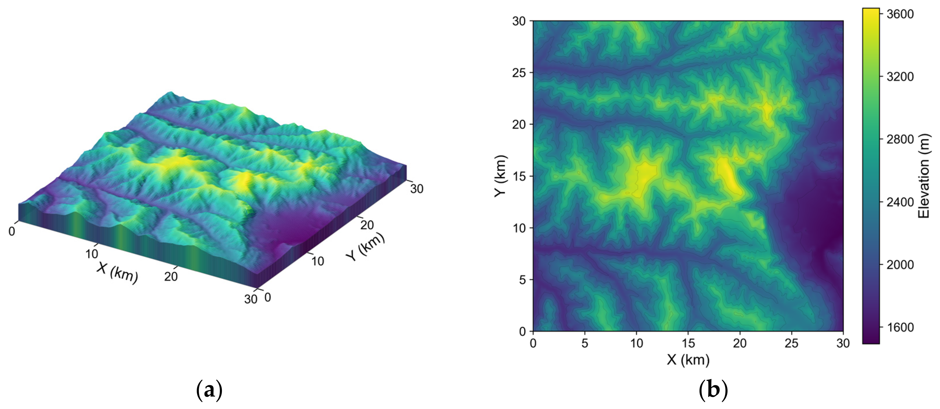
The training terrain covers a 30 km × 30 km region centered at 11.5° N, 39.5° E, derived from the SRTM digital elevation model at a grid resolution of 90 m, as shown in Figure 6.

Figure 6. Elevation visualization of the training terrain. (a) Three-dimensional perspective view; (b) two-dimensional elevation map with the color bar indicating altitude. The terrain is sourced from SRTM and covers 30 km × 30 km.

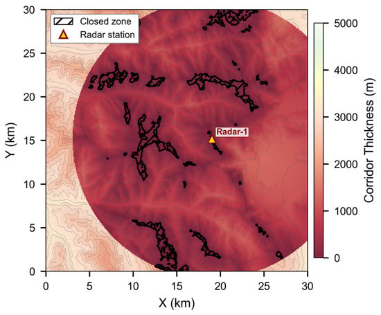
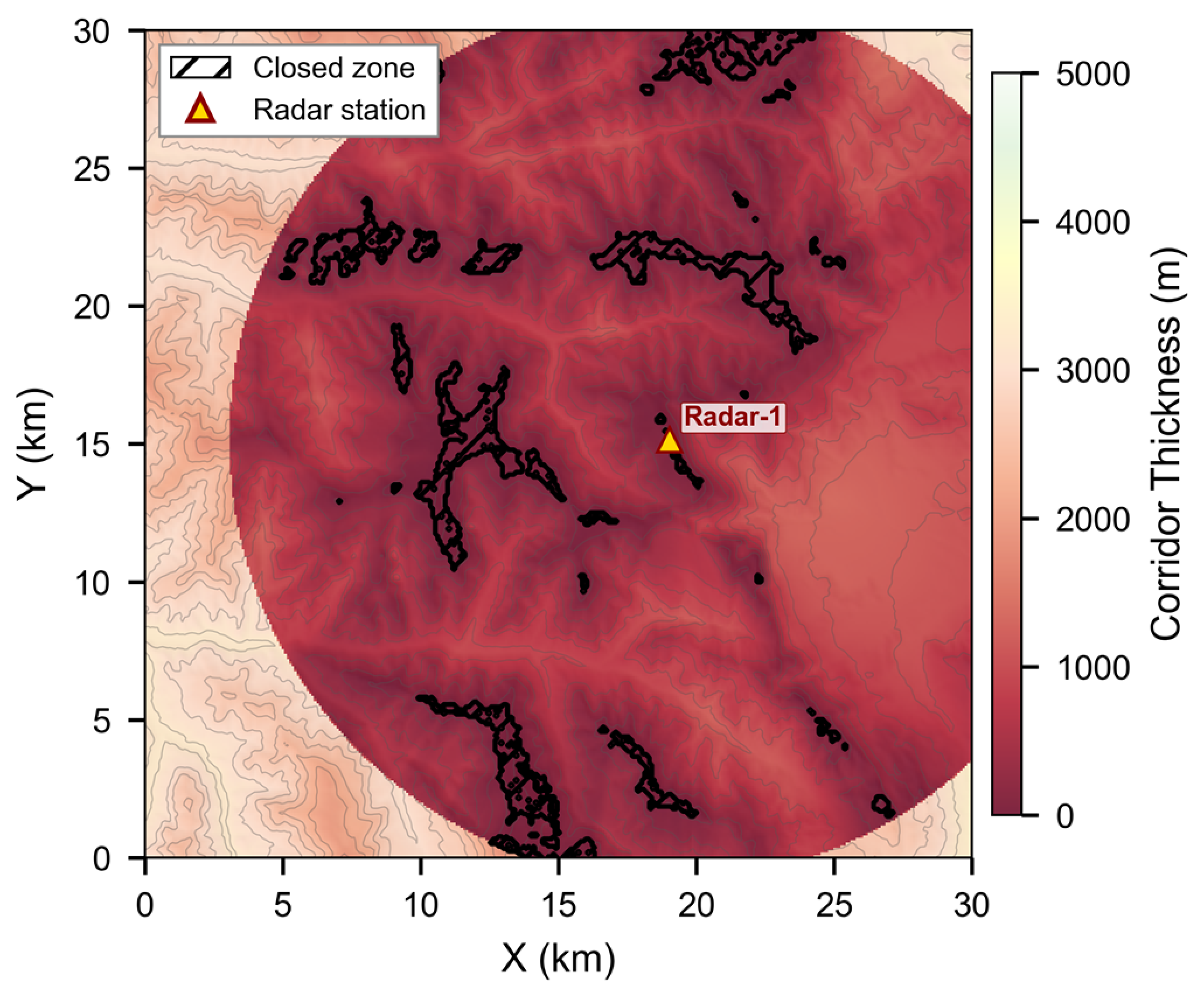
The airspace ceiling within the training region is $h_{\mathrm{A}}=5000$ m. A single radar is deployed with $R_{\mathrm{m}\mathrm{a}\mathrm{x}}=16$ km, ${\theta }_{\mathrm{m}\mathrm{a}\mathrm{x}}=45°$, ${\theta }_{\mathrm{m}\mathrm{i}\mathrm{n}}=-5°$, and an antenna height above ground of 5 m. The radar deployment position and the constraint corridor thickness distribution are shown in Figure 7.

Figure 7. Vertical thickness distribution of the constraint corridor in the training scenario. The color bar indicates corridor thickness; darker regions correspond to smaller thickness, hatched regions mark corridor closures, and triangle markers denote radar positions.

Each episode is reset by generating a start–goal pair together with the initial vehicle state. One of four traversal directions—west-to-east, east-to-west, south-to-north, and north-to-south—is drawn with equal probability. The start is uniformly distributed within the outermost 10% band of the mission region on the near side, and the goal is within the corresponding band on the opposite side. The start altitude is uniformly distributed between 100 m and 500 m above the local terrain, and the goal is placed 500 m above the local terrain.

The vehicle starts in near-level flight roughly heading toward the goal: the flight-path angle is uniformly distributed over a ±2.9° range, the course angle over a ±8.6° range about the direction to the goal, the bank angle and angular rates are zero, and the airspeed is uniformly distributed between 150 m/s and 200 m/s.

The decision interval is set to 0.2 s so that the vehicle advances 30–40 m per decision at cruising speed, less than half the 90 m sampling spacing of the margin field, ensuring that no corridor feature is skipped between consecutive decisions. UAV and environment parameters are listed in Table 3; training hyperparameters are listed in Table 4.

Table 3. UAV and environment parameters.

Parameter	Symbol	Value
Airspace ceiling	$h_{\mathrm{A}}$	5000 m
Decision and integration time step	$\Delta t$	0.2 s
Goal arrival radius	$d_{\mathrm{g}\mathrm{o}\mathrm{a}\mathrm{l}}$	1000 m
Maximum time steps	$T_{\mathrm{m}\mathrm{a}\mathrm{x}}$	2000
Airspeed range	$V_{\mathrm{m}\mathrm{i}\mathrm{n}}$–$V_{\mathrm{m}\mathrm{a}\mathrm{x}}$	150–200 m/s
Maximum bank angle	${\varphi }_{\mathrm{m}\mathrm{a}\mathrm{x}}$	70°
Maximum flight-path angle	${\gamma }_{\mathrm{m}\mathrm{a}\mathrm{x}}$	25°
Maximum roll rate	${\dot{\varphi }}_{\mathrm{m}\mathrm{a}\mathrm{x}}$	90°/s
Maximum flight-path angle rate	${\dot{\gamma }}_{\mathrm{m}\mathrm{a}\mathrm{x}}$	6°/s
Maximum longitudinal acceleration	$a_{\mathrm{m}\mathrm{a}\mathrm{x}}$	5 m/s2
Roll channel gain	$b_{\varphi }$	3.33/s
Flight-path angle channel gain	$b_{\gamma }$	2.0/s
Speed channel gain	$b_V$	0.5/s
Minimum safety clearance	${\delta }_{\mathrm{m}\mathrm{i}\mathrm{n}}$	30 m
Margin normalization reference height	$h_{\mathrm{r}\mathrm{e}\mathrm{f}}$	1000 m
Distance normalization reference	$d_{\mathrm{r}\mathrm{e}\mathrm{f}}$	50 km
Detection intensity shape parameter	$\eta$	0.05

Table 4. Training hyperparameters.

Parameter	Value
Discount factor ${\gamma }_d$	0.99
GAE decay parameter $\lambda$	0.95
Learning rate	3 × 10−4, linearly decayed to 0
Clipping range $ϵ$	0.20
Entropy coefficient	0.0
Value function loss coefficient	0.5
Gradient clipping norm	0.5
Mini-batch size	256
Rollout steps per update (per env)	2048
PPO update epochs $K$	5
Number of parallel environments	8
Total training steps	1 × 107

6.1.2. Evaluation Metrics

The evaluation metrics are organized into four categories. Evaluation is conducted over 100 test episodes. The start–goal pairs are generated once from a fixed random seed following the procedure of Section 6.1.1, and the same set is used by all experiments on the same terrain. In contrast to training, the initial vehicle state is not randomized in evaluation: the vehicle starts in level flight with zero flight-path angle, zero bank angle and zero angular rates, the course angle aligned exactly with the horizontal direction to the goal, and the airspeed set to the midpoint of the admissible range, 175 m/s.

Task completion.

Success rate (SR): the proportion of episodes in which the vehicle reaches the goal.

Collision rate (CR): the proportion of episodes terminated by terrain collision.

Out-of-bounds rate (OOB): the proportion of episodes terminated by horizontal boundary or airspace ceiling exceedance.

Timeout rate (TR): the proportion of episodes exceeding $T_{\mathrm{m}\mathrm{a}\mathrm{x}}$ steps without reaching the goal.

The following three categories are computed only over successful episodes.

Stealth performance.

Detectable equivalent distance (DED) [15]: the cumulative flight distance weighted by detection probability,

$$\mathrm{D}\mathrm{E}\mathrm{D}={\displaystyle \sum _{i=1}^T}\Delta d_i\cdot P_{d,i},$$

(45)

where $\Delta d_i$ is the flight distance at step $i$ and $P_{d,i}$ is the joint detection probability under the independent radar assumption,

$$P_{d,i}=1-{\displaystyle \prod _{k=1}^{N_{\mathrm{R}}}}\left(1-S_{k,i}\right),$$

(46)

where $N_{\mathrm{R}}$ is the number of radars.

Path quality.

Path efficiency (PE): the ratio of the straight-line distance between the start and goal to the actual path length.

Mean AGL: the average above-ground-level altitude of the vehicle along the path.

Average intrusion depth (AID): the mean altitude by which the vehicle exceeds the fused lower detection boundary $h^L$ while within the coverage area:

$$\mathrm{A}\mathrm{I}\mathrm{D}={\displaystyle \frac{1}{\left|\mathcal{I}\right|}}\sum _{i\in \mathcal{I}}\left(h_i-h^L\left(x_i,y_i\right)\right),$$

(47)

where $\mathcal{I}$ is the set of time steps at which the vehicle is within the coverage area and above $h^L$. The average is taken over the episodes for which $\mathcal{I}$ is non-empty.

Computational cost.

Episode computation time (Time): the average total computation time required to complete all decision steps in a single episode.

All experiments are evaluated on the same 100 fixed start–goal pairs under the deterministic initial conditions described above. Policies are trained with three random seeds, and the ± entries of the result tables are sample standard deviations across seeds; they describe dispersion and are not used for inference. Path efficiency, DED, mean AGL and AID are defined only for successful episodes, and the number of successful episodes differs between methods and variants.

6.2. Training Results

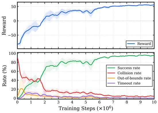
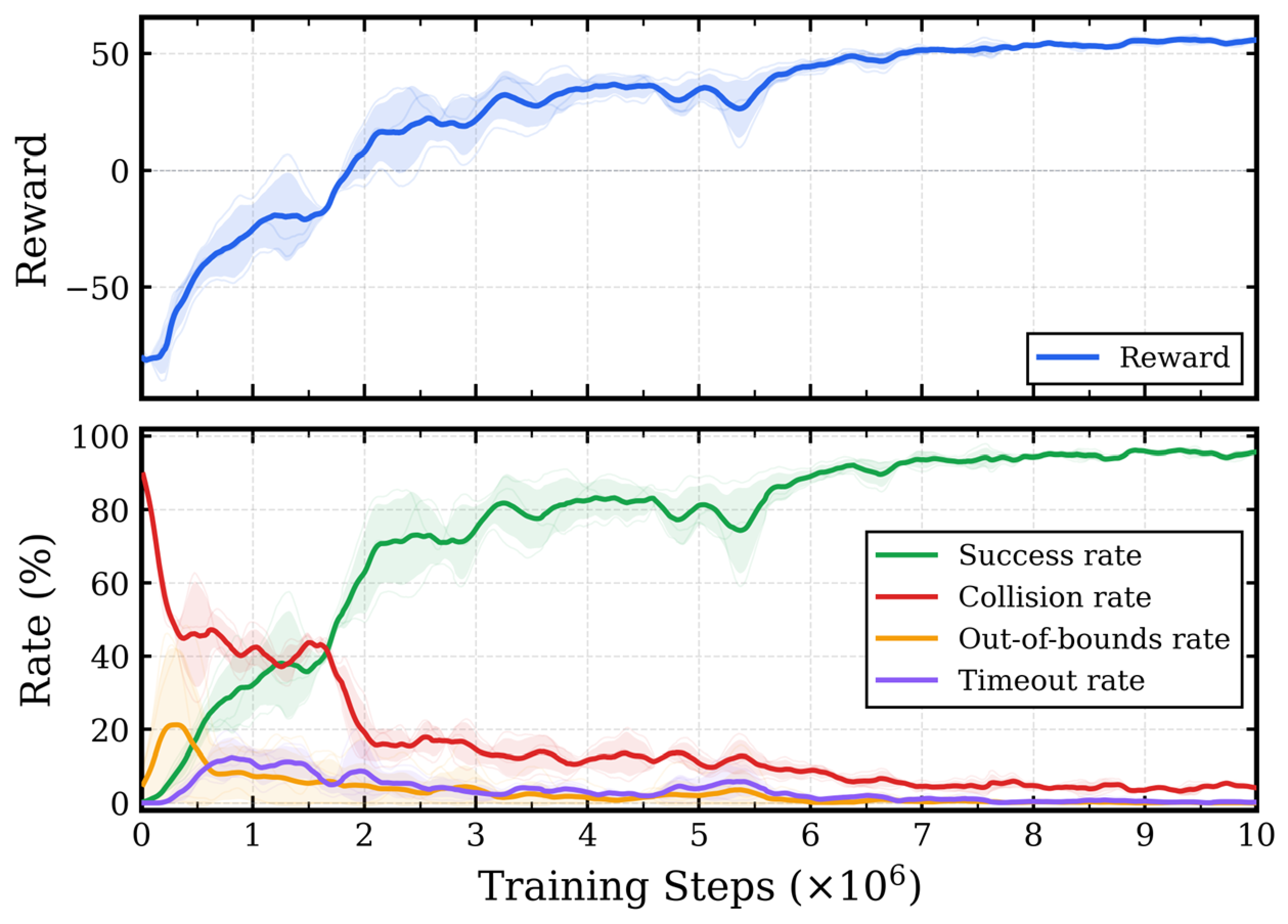
Three independent training runs of $1\times {10}^7$ steps each were conducted with different random seeds. Figure 8 shows the evolution of the mean episode reward and termination metrics over training steps, with shaded bands indicating the standard deviation across seeds. In the first $2\times {10}^6$ steps, the collision rate drops rapidly from approximately 90%, and the success rate rises concurrently to about 70%, indicating that the policy acquires basic navigation capability in this phase. The mean reward plateaus after approximately $6\times {10}^6$ steps; the success rate continues to rise and stabilizes near 95%; the collision rate decreases steadily from its initially high level to approximately 5%; the OOB and timeout rates fall to near zero early in training. The training curves across the three seeds exhibit good consistency, with the inter-seed standard deviation remaining small after convergence.

Figure 8. Training curves. The upper panel shows the mean episode reward; the lower panel shows the termination metrics over training steps. Solid lines are the three-seed mean; shaded bands indicate inter-seed standard deviation.

After training, the final policy of each seed is evaluated on 100 test episodes; the results are summarized in Table 5. Detection exposure is kept at a low level, with a DED of 138.9 m. When traversing radar coverage areas, the average intrusion depth is 56.4 m, indicating that the policy tends to fly at low altitude along terrain-masked regions, staying as much as possible below the fused lower detection boundary. Path efficiency reaches 0.866, meaning the actual path length exceeds the start–goal straight-line distance by about 15%; the policy maintains high navigation efficiency while satisfying corridor constraints. The mean AGL is 392.3 m.

Table 5. Test results on the training terrain (mean ± std over 3 seeds).

Metric	Value
SR (%)	94.0 ± 1.0
CR (%)	5.3 ± 0.6
OOB (%)	0.7 ± 1.2
TR (%)	0.0 ± 0.0
DED (m)	138.9 ± 22.4
PE	0.866 ± 0.018
Mean AGL (m)	392.3 ± 57.5
AID (m)	56.4 ± 4.2

Values are mean ± sample standard deviation over three training seeds, each evaluated on the same 100 test episodes described in Section 6.1.2. DED, PE, Mean AGL and AID are computed over successful episodes; AID is averaged over those episodes in which the vehicle enters the detection envelope.

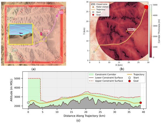
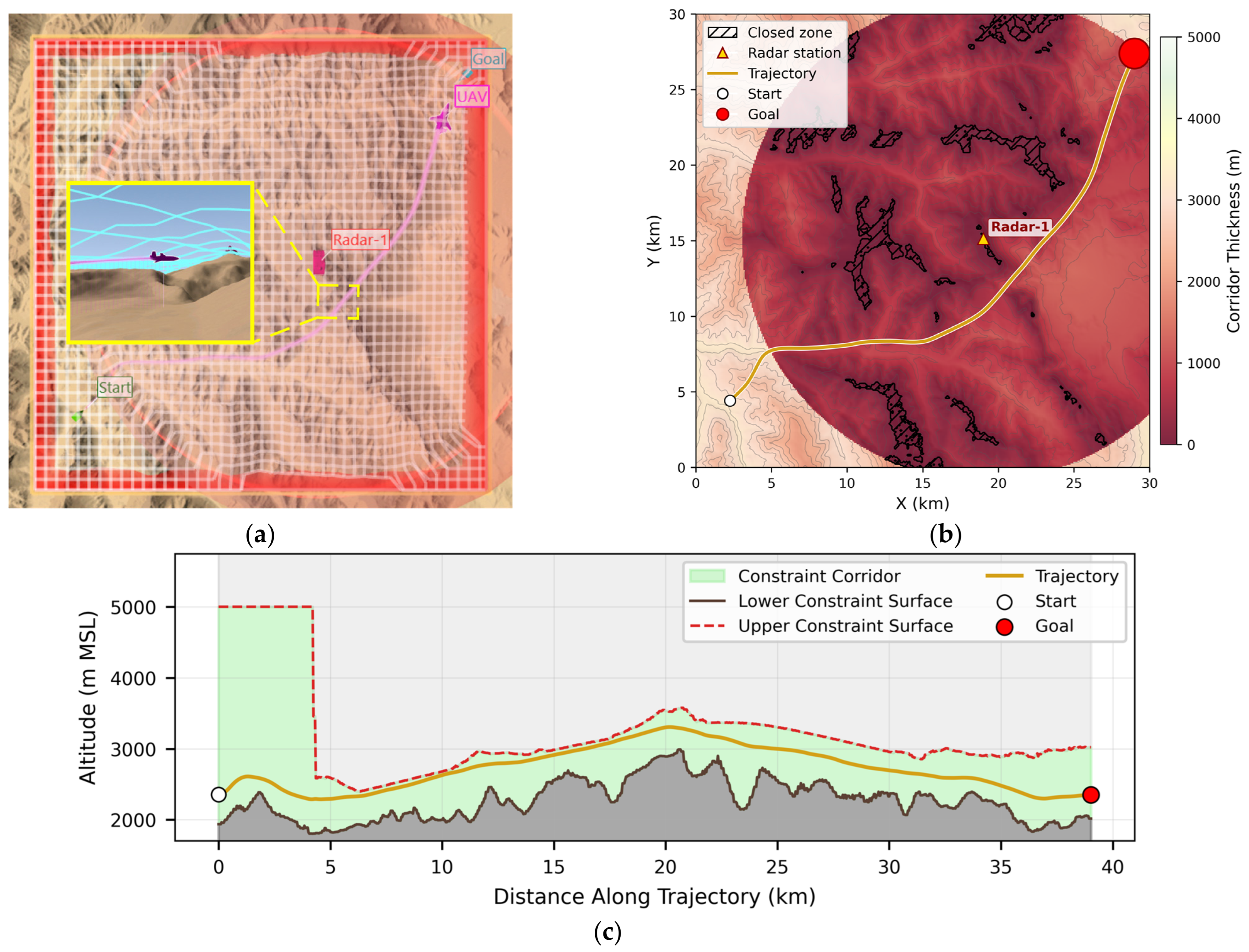
Figure 9 shows a representative trajectory. The three-dimensional perspective view presents the spatial form of the constraint corridor and the flight profile; within the radar coverage area, the corridor’s upper boundary surface closely follows the terrain, compressing the corridor into a narrow spatial layer. The inset provides a close-up of the vehicle navigating through a narrowed corridor segment near the terrain. In the top-down view, the trajectory bypasses closed corridor segments and finds a path through regions where the corridor remains open—a behavior that relies on the margin field’s explicit encoding of corridor closures. The altitude profile shows that after the trajectory enters the radar detection envelope, the fused lower detection boundary replaces the airspace ceiling as the controlling constraint of the corridor’s upper boundary, and the corridor’s vertical thickness drops abruptly from approximately 3000 m to several hundred meters. The policy responds by lowering the flight altitude and flying near the lower boundary within the corridor. At approximately 20 km along the track, the corridor narrows locally, and the trajectory briefly approaches the upper boundary surface. After exiting the narrowed segment, the trajectory returns to the corridor’s mid-region, maintaining vertical clearance to both boundaries.

Figure 9. Representative navigation trajectory. (a) Three-dimensional perspective view showing the spatial form of the constraint corridor and the flight trajectory and attitude of the UAV; (b) top-down view with the trajectory overlaid on the corridor thickness distribution; (c) altitude profile along the track distance, with the light-green region indicating the constraint corridor.

6.3. Comparative Experiments

This section compares ECC-DRL with two representative planning methods to assess its positioning between solution quality and computational cost. The first is three-dimensional voxel A* [15], representing global graph search methods; the second is Dubins-RRT* [17], representing sampling-based planning methods that respect fixed-wing kinematic constraints.

A* searches on the global terrain and fused detection envelope grid. The cost of an edge from node $n_i$ to node $n_j$ is

$$c\left(n_i,n_j\right)=\kappa d_{ij}+\left(1-\kappa \right) S_{\mathrm{m}\mathrm{a}\mathrm{x}}\left(n_j\right) d_{ij},$$

(48)

where $d_{ij}$ is the three-dimensional Euclidean length of the edge, $S_{\mathrm{m}\mathrm{a}\mathrm{x}}\left(n_j\right)=\underset{k}{\max }{S}_k\left(n_j\right)$ is the largest per-radar detection intensity of Equation (19) at the arrival node, and $\kappa \in (0,1]$ is the weight: smaller $\kappa$ increases the weight of stealth, biasing the search toward paths with lower detection exposure but greater length; larger $\kappa$ increases the weight of path length, favoring shorter but more exposed paths. Both terms carry the dimension of length, and $S_{\mathrm{m}\mathrm{a}\mathrm{x}}\in \left[0,1\right]$ bounds the second term by the first, so $\kappa$ alone determines the trade-off. The aggregation of the radars by the maximum in Equation (48) is a monotone surrogate for the joint detection probability of Equations (45) and (46); it affects which paths A* prefers, not how they are scored, since all three methods are scored by the same metrics of Section 6.1.2.

Dubins-RRT* runs RRT* with Dubins airplane motion primitives, enforces safety verification to ensure the path does not enter inevitable-collision states, and requires the entire path to remain within the constraint corridor. At the maximum bank angle ${\varphi }_{\mathrm{m}\mathrm{a}\mathrm{x}}$ of Table 3 and the mid-range airspeed of 175 m/s, Equation (3) gives a minimum turn radius of 1136 m. Motion primitives exceeding the maximum extension are truncated along the primitive itself, so that the heading at the truncation point remains tangent to the path. The near set used in the choose-parent and rewiring steps is of the k-nearest form. As an anytime planner, Dubins-RRT* is stopped by a single criterion, a budget of 150 s per episode, chosen to be of the same order as the solution times of A*.

The settings of the two baseline planners are listed in Appendix A, Table A1. All three methods are evaluated on the same 100 test episodes of Section 6.1.2. Table 6 lists the quantitative results of each method.

Table 6. Comparative experimental results.

Method	SR (%)	DED (m)	PE	Mean AGL (m)	AID (m)	Time (s)
ECC-DRL (ours)	94.0 ± 1.0	138.9 ± 22.4	0.866 ± 0.018	392.3 ± 57.5	56.4 ± 4.2	1.30 ± 0.08
A* (κ = 0.1)	100.0	19.8 ± 33.7 †	0.933 ± 0.021 †	355.0 ± 88.8 †	17.9 ± 24.8 †	54.53
A* (κ = 0.2)	100.0	36.9 ± 59.8	0.936 ± 0.021	356.8 ± 90.9	21.0 ± 26.0	66.82
A* (κ = 0.3)	100.0	65.5 ± 110.5	0.938 ± 0.019	360.6 ± 90.8	26.0 ± 24.6	76.50
A* (κ = 0.4)	100.0	133.5 ± 250.4	0.942 ± 0.020	358.0 ± 94.0	34.6 ± 58.2	84.53
A* (κ = 0.5)	100.0	187.9 ± 320.3	0.943 ± 0.020	361.0 ± 100.1	39.7 ± 59.1	92.18
A* (κ = 0.6)	100.0	229.0 ± 347.3	0.944 ± 0.020	364.2 ± 90.9	55.8 ± 68.0	102.86
A* (κ = 0.7)	100.0	301.2 ± 393.9	0.945 ± 0.021	386.6 ± 99.3	67.1 ± 77.3	113.78
A* (κ = 0.8)	100.0	358.9 ± 461.9	0.946 ± 0.021	371.5 ± 96.7	76.6 ± 79.1	122.95
A* (κ = 0.9)	100.0	616.4 ± 692.6	0.947 ± 0.021	388.7 ± 101.3	101.8 ± 94.9	135.10
A* (κ = 1.0)	100.0	4445.3 ± 3374.8	0.949 ± 0.022	485.8 ± 132.9	199.3 ± 107.0	139.30
Dubins-RRT*	100.0 ± 0.0	0.4 ± 0.3	0.738 ± 0.004	643.1 ± 8.3	10.3 ± 9.3	150

The statistical basis is given in Section 6.1.2 and Section 6.3; entries marked † denote the standard deviation across the 100 test episodes rather than across runs, and apply to all A* rows. For ECC-DRL, each seed contributes the mean over its own successful episodes, and the entry is the mean ± sample standard deviation of the three seed means. AID is averaged over those episodes in which the vehicle enters the detection envelope; the number of such episodes differs between methods and, for A*, between values of $\kappa$. Time denotes cumulative policy inference over all decision steps of one episode for ECC-DRL, and measured single-query planning time for A*. For Dubins-RRT*, Time denotes the per-query planning budget, which is the sole stopping criterion; the planner runs in anytime mode and always exhausts the budget, so all reported quality metrics correspond to the solution held at 150 s.

A* is deterministic and is run once, so the ± entries of its rows in Table 6 are standard deviations across the 100 test episodes rather than across runs; Dubins-RRT* is run three times with different sampling seeds. Comparisons of path efficiency between methods are made on the 89 episodes solved by ECC-DRL under all three seeds, by pairing at the episode level, with the per-episode value of ECC-DRL averaged over its three seeds and that of Dubins-RRT* over its three runs. Paired differences are summarised by the mean difference and a 95% percentile bootstrap confidence interval over 20,000 resamples of the episodes. A comparison conditioned in this way does not reflect the difference in success rate, which is reported separately.

Across the entire $\kappa$ range, the path efficiency of A* remains stable between 0.933 and 0.949, while the DED spans two orders of magnitude, from 19.8 m to 4445.3 m; A* therefore maintains high path efficiency at all stealth levels. The DED of ECC-DRL is 138.9 m, of the same order as the 133.5 m of A* at $\kappa =0.4$, providing a working point at which path efficiency can be compared at a comparable level of average detection exposure. At this working point, the path efficiency of ECC-DRL is 0.866, reaching 91.9% of the 0.942 achieved by A*; over the 89 episodes solved by ECC-DRL under all three seeds, the paired difference is $-0.073$ (95% CI $\left[-0.092, -0.055\right]$). Considering that A* uses complete global information for offline computation while ECC-DRL makes online decisions from local margin fields alone, this indicates that ECC-DRL generates flight paths approaching that of a globally informed A*. In terms of success rate, A* achieves 100% and ECC-DRL 94.0%, and among the 100 test episodes there is no episode in which ECC-DRL succeeds and A* fails. A* searches with complete global information and is guaranteed to find a feasible path in a connected environment; as a reactive policy, ECC-DRL may lack sufficient look-ahead in scenarios where the corridor narrows abruptly, and the vehicle needs to adjust altitude well in advance.

Dubins-RRT* achieves extremely low detection exposure by enforcing the entire path to stay within the constraint corridor, yielding a DED of 0.4 m and a mean AID of 10.3 m. However, the joint restriction of kinematic constraints and corridor safety verification compresses the feasible sampling space, resulting in a path efficiency of 0.738 against 0.866 for ECC-DRL; over the 89 episodes solved by ECC-DRL under all three seeds, the paired difference is $+0.130$ (95% CI $\left[+0.106, +0.154\right]$). The two methods occupy different points of the same trade-off: Dubins-RRT* attains a detection exposure two orders of magnitude below that of ECC-DRL by confining the entire path to the corridor, at the cost of path efficiency, whereas ECC-DRL accepts a detection exposure of 138.9 m and retains the higher path efficiency of the two. Within the 150 s budget, Dubins-RRT* returns a feasible path in all test episodes, as does A*, confirming that path connectivity between start and goal is established in every case; as with A*, there is no episode in which ECC-DRL succeeds and Dubins-RRT* fails.

The three methods differ fundamentally in when their computation must be performed. ECC-DRL is the only one of the three that operates online within the decision interval: its per-step computation completes within the 200 ms decision interval, with a measured end-to-end maximum of 10.17 ms on the embedded platform (Section 6.6), and the cumulative inference time over all decision steps of a single episode is 1.30 s. Both A* and Dubins-RRT* must instead complete their computation offline in advance, at a cost two to three orders of magnitude above the decision interval: A* requires 54.53–139.30 s for a single search, increasing monotonically with $\kappa$ as the heuristic departs from the straight-line distance and the search space expands, and Dubins-RRT* is run under a 150 s budget. This difference stems from a fundamental distinction in computational paradigm: planning methods must solve for a complete path from start to goal in a global search space, with computational cost growing with the search space scale; the policy network of ECC-DRL performs only a single forward pass at each decision step, and the per-step inference time is independent of the environment scale.

Taken together, these results position ECC-DRL as trading approximately 8% of path efficiency for online operation within the decision interval, while maintaining average detection exposure of the same order as A* at $\kappa =0.4$. A* attains lower detection exposure than ECC-DRL only for $\kappa \le 0.4$ where its search time is already 54.53–84.53 s.

6.4. Ablation Study

To verify the necessity of the egocentric margin field and the individual contributions of the upper and lower margin fields, three ablation variants are designed; their configurations are listed in Table 7. The w/o ${\mathbf{M}}^U$ and w/o ${\mathbf{M}}^L$ variants each remove one margin field channel to isolate the contribution of each channel. The Vector-only variant removes all margin field branches to verify the necessity of the spatial field information provided by ECC beyond the scalar information already present in the vector state. When a margin field branch is removed, the corresponding per-source margin scalars in the vector state are retained, so that the ablation removes spatial field information rather than all perception of that constraint dimension. All variants share the same reward function, action space, and training hyperparameters, and each is trained independently with the same three random seeds. Table 8 reports the evaluation results.

Table 7. Ablation variant configurations.

Variant	${\mathbf{M}}^{\mathit{L}}$	${\mathbf{M}}^{\mathit{U}}$	${\mathbf{s}}^{\mathbf{v}\mathbf{e}\mathbf{c}}$
ECC-DRL	✓	✓	✓
w/o ${\mathbf{M}}^U$	✓	✗	✓
w/o ${\mathbf{M}}^L$	✗	✓	✓
Vector only	✗	✗	✓

✓ indicates that the component is retained; ✗ indicates that it is removed.

Table 8. Ablation results (mean ± std over 3 seeds).

Variant	SR (%)	CR (%)	OOB (%)	TR (%)	DED (m)	PE	Mean AGL (m)	AID (m)
ECC-DRL	94.0 ± 1.0	5.3 ± 0.6	0.7 ± 1.2	0.0 ± 0.0	138.9 ± 22.4	0.866 ± 0.018	392.3 ± 57.5	56.4 ± 4.2
w/o ${\mathbf{M}}^U$	88.7 ± 9.3	9.7 ± 9.8	0.0 ± 0.0	1.7 ± 1.2	324.6 ± 17.5	0.783 ± 0.032	346.6 ± 28.4	65.6 ± 9.2
w/o ${\mathbf{M}}^L$	77.3 ± 8.5	10.3 ± 3.1	4.0 ± 6.1	8.3 ± 4.2	737.1 ± 123.1	0.789 ± 0.024	511.0 ± 18.8	72.8 ± 4.1
Vector only	22.7 ± 8.0	65.7 ± 8.3	11.7 ± 12.5	0.0 ± 0.0	2972.5 ± 780.9	0.887 ± 0.059	546.8 ± 11.3	113.3 ± 26.3

Values are mean ± sample standard deviation over three training seeds, each evaluated on the same 100 test episodes. DED, PE, Mean AGL and AID are computed over successful episodes, the number of which differs between variants; AID is averaged over those episodes in which the vehicle enters the detection envelope.

The comparison between removing the upper margin field and removing the lower margin field reveals how the nature of each constraint influences the demand for spatial field information. In the training scenario, the lower margin field encodes terrain constraints—terrain collision terminates the episode and thus constitutes a hard constraint; the upper margin field primarily encodes the fused radar lower detection boundary within coverage areas—entering the detection region incurs a per-step penalty but does not terminate flight, constituting a soft constraint.

After removing the lower margin field branch, the success rate drops by 16.7 percentage points to 77.3%, and the drop is present in every seed (87.0%, 71.0% and 74.0%, against 95.0%, 93.0% and 94.0% for the full model). Without spatial terrain information, the policy cannot anticipate terrain changes ahead. The additional failures are dominated by timeouts (8.3%) and out-of-bounds terminations (4.0%) rather than by collisions, which remain at 10.3%: the policy compensates for the missing terrain preview by climbing, raising the mean AGL from 392.3 m to 511.0 m, and the resulting detours exhaust the step budget or carry the vehicle beyond the mission region. The higher altitude also makes the vehicle more likely to enter radar detection regions, causing DED to increase to 737.1 m—a stealth degradation greater than the 324.6 m observed when removing the upper margin field branch.

After removing the upper margin field branch, the success rate shows no systematic change (88.7 ± 9.3%). The three seeds yield 78.0%, 95.0% and 93.0%, so the reduction in the mean is attributable to a single seed rather than to the ablation itself. The degradation of this variant is instead concentrated in stealth and path quality, where it is consistent across seeds: DED rises from 138.9 m to 324.6 m, AID from 56.4 m to 65.6 m, and path efficiency falls from 0.866 to 0.783. The loss of spatial information about the radar detection envelope prevents the policy from effectively exploiting terrain-masked regions; because radar detection is a soft constraint, however, the vehicle can continue flying and reach the goal even after entering the detection region, which is consistent with the success rate being unaffected. The mean AGL of this variant is 346.6 m; retaining the lower margin field allows the policy to continue flying close to the terrain, which partly suppresses further stealth degradation through terrain masking.

The path efficiency of the two single-channel variants is 0.783 and 0.789, respectively, against 0.866 for the full model, indicating that removing either egocentric margin field impairs navigation efficiency.

After removing all margin field branches, the policy relies solely on the per-source margin scalars and other flight state information in the vector state. The success rate of this variant is only 22.7% with a collision rate as high as 65.7% and a DED of 2972.5 m. Per-source margin scalars provide only the vertical clearance to each constraint source at the vehicle’s current position and contain no spatial information about the surrounding corridor; the policy cannot foresee upcoming terrain undulations or corridor narrowing, leading to numerous terrain collisions. The path efficiency of this variant is 0.887, apparently close to the 0.866 of the full model; this value is, however, computed over only the 22.7% of episodes that succeed, which are those with relatively relaxed constraints, and it is therefore not comparable with the value of the full model, which is computed over 94.0% of the episodes.

In summary, the ablation study yields two key findings. First, spatial margin fields are a necessary condition for reliable corridor navigation. The Vector-only variant relies solely on per-source margin scalars at the vehicle’s current position. These scalars reflect only the instantaneous vertical clearance to each constraint source and contain no information about the spatial structure of the surrounding corridor, leaving the policy unable to anticipate upcoming terrain undulations or corridor narrowing. The resulting success rate of 22.7% with a collision rate of 65.7% confirms that the upgrade from scalar to spatial field representation provided by ECC is indispensable. Second, both margin field channels contribute, but through different mechanisms and to different metrics. Removing the lower margin field, which in this scenario encodes the terrain hard constraint, reduces the success rate by 16.7 percentage points on average, with a reduction present in every seed; the policy is forced to increase flight altitude to reduce collision risk, and the higher altitude in turn exposes the vehicle to the radar detection region, causing DED to worsen from 138.9 m to 737.1 m in a cascading effect. Removing the upper margin field, which encodes the radar soft constraint, leaves the success rate unchanged—consistent with the fact that detection penetration does not terminate the episode—but degrades stealth performance substantially, with DED increasing from 138.9 m to 324.6 m. This indicates that the upper margin field is necessary for the policy to exploit terrain-masked regions for detection avoidance. The path efficiency of both single-channel removal variants falls to approximately 0.78, confirming that the removal of either channel impairs navigation efficiency.

6.5. Zero-Shot Transfer

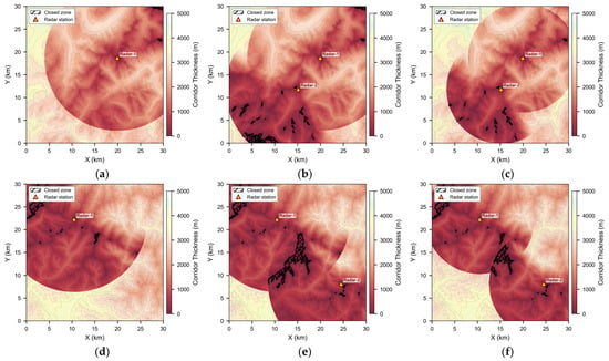
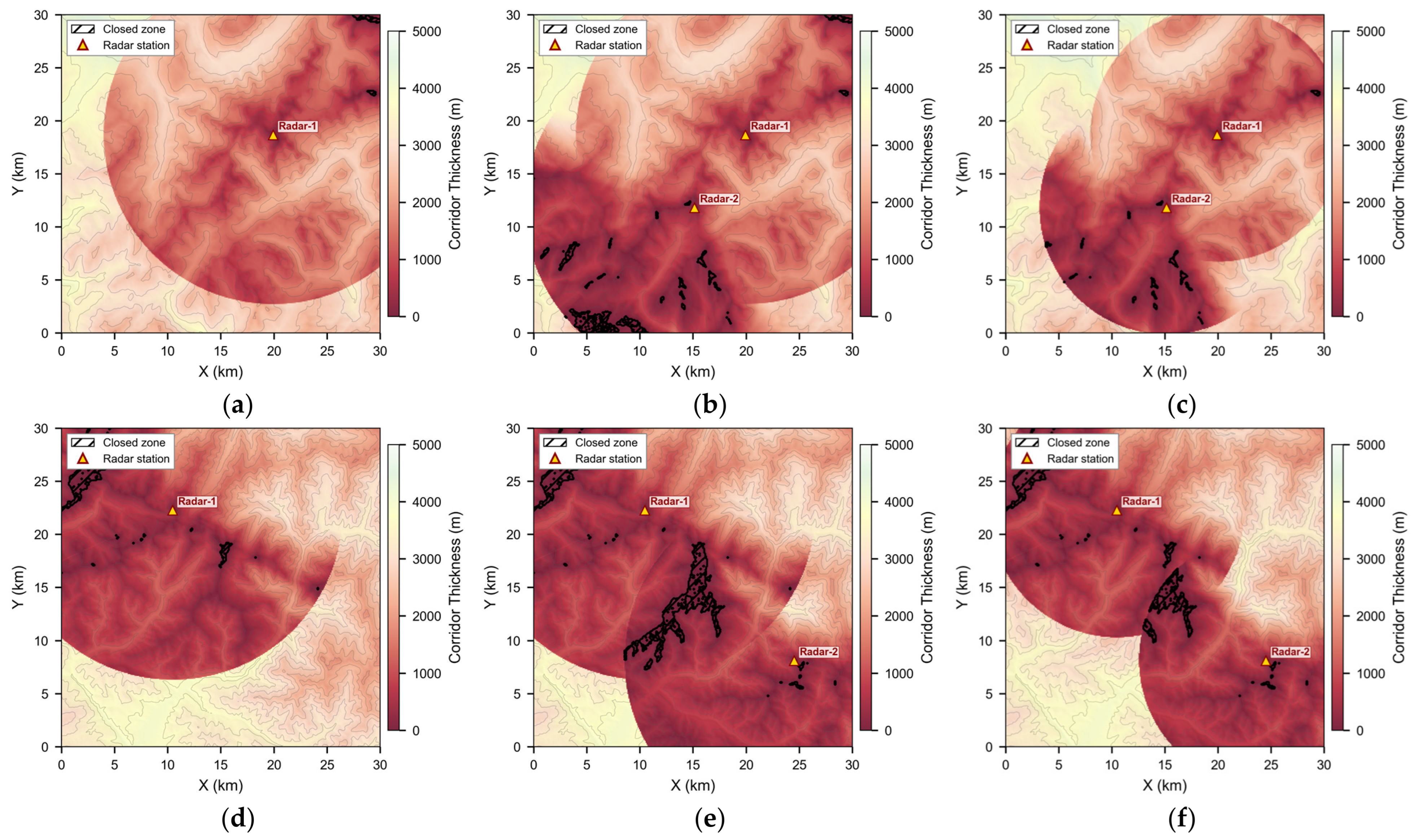
All settings follow the training scenario in Section 6.1.1 except for the terrain elevation data and the radar deployment. To verify the cross-scenario transfer capability conferred by egocentric encoding, a policy trained with a single seed is tested zero-shot on six scenarios formed by combining two unseen terrains with three radar configurations, without any retraining or fine-tuning. Both test terrains are derived from SRTM and cover a 30 km × 30 km area: Terrain A is centered at 45.8° N, 6.8° E; Terrain B is centered at 42.5° N, 44.0° E. The three radar configurations are a single radar with $R_{\mathrm{m}\mathrm{a}\mathrm{x}}=16$ km, two radars with $R_{\mathrm{m}\mathrm{a}\mathrm{x}}=16$ km, and two radars with $R_{\mathrm{m}\mathrm{a}\mathrm{x}}=12$ km; the elevation angle range and antenna height of each radar are identical to those of the training radar. The corridor thickness distributions of the six scenarios are shown in Figure 10, and Table 9 lists the evaluation results.

Figure 10. Corridor thickness distributions of the six zero-shot transfer test scenarios. (a–c) Terrain A; (d–f) Terrain B. Triangle markers denote radar positions; hatched regions mark corridor closures.

Table 9. Zero-shot transfer results across unseen scenarios.

Scenario	Terrain	Radar	SR (%)	CR (%)	OOB (%)	TR (%)	DED (m)	PE	Mean AGL (m)	AID (m)
1	A	1 × 16 km	90.3 ± 3.2	8.3 ± 2.1	1.0 ± 1.0	0.3 ± 0.6	0.4 ± 0.7	0.954 ± 0.014	719.5 ± 250.9	n/a
2	A	2 × 16 km	88.3 ± 2.1	10.0 ± 1.0	1.3 ± 1.5	0.3 ± 0.6	93.7 ± 11.0	0.940 ± 0.007	661.7 ± 210.8	47.6 ± 6.7
3	A	2 × 12 km	88.7 ± 0.6	10.3 ± 0.6	0.7 ± 1.2	0.3 ± 0.6	56.6 ± 12.6	0.942 ± 0.009	669.8 ± 207.4	41.5 ± 7.1
4	B	1 × 16 km	83.7 ± 3.1	15.0 ± 2.0	1.3 ± 2.3	0.0 ± 0.0	121.1 ± 17.6	0.939 ± 0.003	544.4 ± 126.1	49.3 ± 12.7
5	B	2 × 16 km	79.3 ± 4.2	19.7 ± 4.0	1.0 ± 1.7	0.0 ± 0.0	439.1 ± 61.4	0.893 ± 0.016	480.6 ± 85.0	61.9 ± 2.6
6	B	2 × 12 km	84.7 ± 3.8	14.7 ± 3.2	0.7 ± 1.2	0.0 ± 0.0	285.8 ± 63.2	0.921 ± 0.007	510.7 ± 110.4	76.8 ± 6.4

Values are mean ± sample standard deviation over the three policies of Section 6.2, each evaluated on 100 test episodes per scenario. DED, PE, Mean AGL and AID are computed over successful episodes; AID is averaged over those episodes in which the vehicle enters the detection envelope, and is reported as n/a for Scenario 1, in which no episode enters it.

The policy achieves success rates of 79.3% to 90.3% across the six unseen scenarios, with timeout terminations occurring in at most 0.3% of episodes. Failures are predominantly terrain collisions, with a small number of episodes terminated by horizontal boundary exceedance; the failure modes are consistent with those observed on the training terrain. Path efficiency ranges from 0.893 to 0.954, indicating that the policy maintains high navigation efficiency in unseen scenarios. The three Terrain B scenarios have overall lower success rates than Terrain A; as shown in Figure 10, Terrain B exhibits a larger and more concentrated corridor closure area, and the difference in success rates is consistent with the difference in corridor constraints.

The mean AGL is the one metric whose inter-seed standard deviation is large: in Scenario 1, the three seeds give 1008.6 m, 558.5 m and 591.4 m, and a similar spread is observed in the remaining scenarios. This reflects a difference in the cruising altitude adopted by the three policies rather than measurement noise, and it propagates to the detection exposure, since a policy that cruises higher is more likely to enter the detection envelope. The success rates of the three seeds remain within a few percentage points of one another in every scenario, so the transfer capability itself is not affected.

These results demonstrate that a policy trained on a single terrain with a single radar can transfer to unseen terrains and radar deployments without retraining. This transfer capability stems from the egocentric encoding described in Section 4.2: the margin field depends only on the relative geometry between the vehicle and the surrounding corridor, decoupled from the global position and absolute heading, so that geometrically similar corridor segments in different scenarios produce similar margin field inputs and the policy makes consistent decisions accordingly.

6.6. Hardware-in-the-Loop Experiment

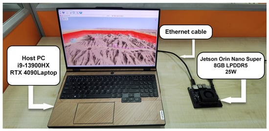
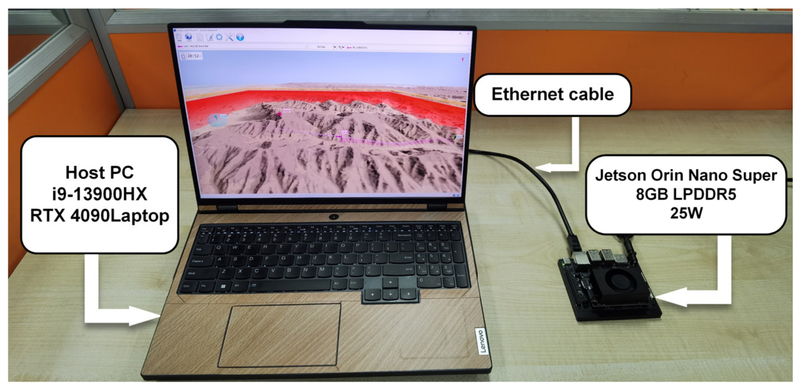
This section conducts a hardware-in-the-loop (HIL) experiment on an NVIDIA Jetson Orin Nano Super (NVIDIA, Santa Clara, CA, USA) to verify whether the policy can meet real-time constraints on an embedded platform. The platform is equipped with a 1024-core Ampere GPU and 8 GB LPDDR5 memory, operating at a power budget of 25 W.

The HIL experiment places the simulation environment and onboard inference on two separate hardware platforms. The host runs the simulation environment and sends the flight state to the Jetson via Ethernet at each decision step; the Jetson receives the state, constructs the margin field and vector state, performs policy inference, and returns the action to the host to advance the simulation, forming a closed loop. The experimental setup is shown in Figure 11.

Figure 11. Hardware-in-the-loop experimental setup. The host runs the simulation environment and communicates with the NVIDIA Jetson Orin Nano Super via Ethernet; the Jetson performs observation construction and policy inference.

The policy network is exported from PyTorch to the ONNX intermediate format and then converted to a half-precision floating-point (FP16) inference engine by NVIDIA TensorRT 10.7 to reduce memory footprint and accelerate inference. The statistical results of the end-to-end computation latency, measured in closed loop over all decision steps of the 100 test episodes, are listed in Table 10. The mean latency is 3.93 ms, and the P95 is 4.33 ms; the maximum of 10.17 ms is an outlier against a standard deviation of only 0.44 ms, and all values remain well below the decision time step of $\Delta t=200$ ms. Observation construction accounts for approximately 73% of the total latency; the online sampling and interpolation of the margin field constitute the primary computational bottleneck of the inference pipeline.

Table 10. End-to-end computation latency.

Stage	Mean (ms)	Std (ms)	P95 (ms)	Max (ms)
Observation construction	2.87	0.29	3.13	4.29
Policy inference	1.06	0.33	1.31	7.16
End-to-end total	3.93	0.44	4.33	10.17

Statistics are computed over 81,677 decision steps of the 100 evaluation episodes, with the first 100 steps discarded as warm-up.

Table 11 compares the closed-loop navigation performance of a policy trained with a single seed on the PC and the Jetson, evaluated on the same 100 test episodes with the same initial vehicle state, so that the two runs differ only in where the observation construction and the policy inference are executed and in which numerical precision. The two runs give identical task-completion statistics, and the agreement holds episode by episode: all 100 episodes terminate in the same manner, and 90 of them have exactly the same length; FP16 quantization does not alter the closed-loop behavior of the policy. These results demonstrate that both observation construction and policy inference of ECC-DRL can be completed in real time on an embedded platform, meeting the latency requirements for closed-loop deployment.

Table 11. PC vs. HIL closed-loop performance.

Metric	PC (PyTorch FP32)	HIL (TensorRT FP16)
SR (%)	94.0	94.0
CR (%)	6.0	6.0
OOB (%)	0.0	0.0
TR (%)	0.0	0.0

7. Discussion

The egocentric margin field supplies the corridor structure that is required for reliable decisions in vertically constrained airspace. A narrowing of the feasible altitude interval may originate either from the upper boundary descending or from the lower boundary rising, and the two call for opposite avoidance responses. Retaining the complete two-sided margin information allows the policy to distinguish between them; removing one channel leaves the policy without information on the boundary that channel encodes, and reducing the observation to a scalar clearance removes the corridor structure from the observation altogether.

The comparison with the two planning methods reveals differences of two distinct origins. Relative to globally informed A*, the difference originates in the information available: A* searches over the complete constraint map, whereas ECC-DRL decides from egocentric local observations alone and, in configurations calling for a long-range detour, can select its turning point only from the corridor geometry within the current neighborhood. At a working point of comparable detection exposure, its path efficiency approaches that of A*, and the remaining gap is the price of this locality. Relative to Dubins-RRT*, the difference originates in how the constraint is handled: confining the entire path to the corridor under fixed-wing kinematic constraints compresses the feasible sampling space, yielding very low detection exposure at reduced path efficiency, whereas ECC-DRL treats the margin as a continuous quantity to be traded off.

7.1. Limitations

The margin field projects the vertical constraints onto a two-dimensional horizontal sampling grid, retaining one pair of upper and lower boundary values at each grid point. It therefore applies where the vertical free space at any horizontal position forms a single interval, as with terrain surfaces, radar detection envelopes, and no-fly volumes of definite ceiling and floor. Where multiple vertical free spaces coexist at one horizontal position, as in bridges passed underneath, multi-level structures, or enclosed tunnels, a single-interval representation cannot distinguish the available passages, and the present form of the ECC is not directly applicable to general three-dimensional volumetric obstacles.

The kinematic model and all experiments reported here are set in wind-free conditions. Crosswind and vertical gusts displace the actual flight path from the commanded one and alter the available climb rate, and because the ECC defines a corridor of limited vertical margin, the consequences are more immediate than in open airspace; terrain-induced disturbances are common in low-altitude terrain-following flight [38]. The observation likewise presumes exact knowledge of the vehicle state and of the constraint-source parameters, whose errors shift the constructed boundary surfaces as a whole, a shift the policy cannot distinguish from the observation. Variations of platform mass and aerodynamic characteristics further alter the attainable climb rate and turn radius.

The hardware-in-the-loop experiments verify feasibility at the computational level: the end-to-end maximum latency of observation construction and policy inference is 10.17 ms, a small fraction of the 200 ms decision interval. Dynamic robustness under real flight conditions lies outside their scope, and a policy verified in simulation alone may degrade under real wind disturbance, sensor noise, actuator delay, and modeling error.

7.2. Future Work

The representation admits extension in two directions. Extending each horizontal grid point from a single interval to several vertical free intervals would cover general three-dimensional volumetric obstacles, at the cost of altering the observation and introducing a passage-selection decision into the action space. The second concerns the sampling geometry. A sampling grid of fixed extent and spacing couples the near-field resolution of the margin field to its look-ahead range, since at a given input dimension one can be extended only at the expense of the other. Encodings whose spatial scale adapts to the vehicle state and to the local corridor geometry would relax this coupling and are a natural direction for extending the representation.

Progress toward real environments can proceed in three steps: bringing wind into the framework, for instance through a wind estimate in the observation or a wind-dependent safety margin; applying domain randomization over wind, sensor noise, aerodynamic coefficients, and actuation delay during training, and repeating the present metric set over a grid of disturbance magnitudes to characterize how performance degrades with disturbance strength; and outdoor flight testing on a scaled platform.

The simulation approximates the closed-loop response of the autopilot as a first-order system with fixed time constants, so the tracking lag of the inner loop is modeled while its variation with flight state and actuator saturation is not, and the bandwidth itself is not treated as a design quantity. Within a corridor of limited vertical margin, tracking lag translates directly into altitude error, an effect that grows as the corridor narrows. Existing research on inner-loop flight control has concentrated on fault-tolerant control under complex flight conditions [39] and on the optimization of convergence performance [40]. Prescribed-time and fixed-time designs are of particular relevance here, since they render the settling time of the inner loop a constant assigned by the designer; pairing the present guidance policy with an inner loop of this class would therefore make the settling time assumed here a quantity guaranteed by the control law rather than an approximation adopted for simulation.

8. Conclusions

This paper proposed the Egocentric Constraint Corridor (ECC), which fuses heterogeneous multi-source constraints into upper and lower boundary surfaces to define a constraint corridor via constraint fusion, then egocentrically encodes the surrounding corridor as an egocentric margin field, and builds on this representation an end-to-end deep reinforcement learning navigation framework whose multi-branch network and composite reward function follow from the structure of the corridor encoding. The approach was systematically validated in a fixed-wing low-altitude penetration scenario, against both a global graph-search planner and a sampling-based planner respecting fixed-wing kinematics. Experimental results show that the egocentric margin field provides corridor constraint information that is necessary for reliable navigation, and that egocentric encoding endows the policy with cross-scenario generalization capability, enabling zero-shot transfer to scenarios with unseen terrains and radar deployments without retraining or fine-tuning. ECC-DRL attains path efficiency approaching that of a globally informed A* at a comparable level of average detection exposure, while being the only one of the compared methods that computes its decisions online within the decision interval, and satisfies the latency requirements for real-time closed-loop operation on a resource-constrained embedded platform. The corridor abstraction underlying this framework is independent of the origin of the constraints it fuses, and the results reported here suggest that it offers a workable basis for learning-based navigation in vertically constrained airspace.

References

- Huang, H.; Su, J.; Wang, F.-Y. The Potential of Low-Altitude Airspace: The Future of Urban Air Transportation. IEEE Trans. Intell. Veh. 2024, 9, 5250–5254. [Google Scholar] [CrossRef] [Scilit]
- Ahmed, S.S.; Fountas, G.; Lurkin, V.; Anastasopoulos, P.C.; Zhang, Y.; Bierlaire, M.; Mannering, F. The State of Urban Air Mobility Research: An Assessment of Challenges and Opportunities. IEEE Trans. Intell. Transp. Syst. 2025, 26, 1375–1394. [Google Scholar] [CrossRef] [Scilit]
- Mohsan, S.A.H.; Khan, M.A.; Noor, F.; Ullah, I.; Alsharif, M.H. Towards the Unmanned Aerial Vehicles (UAVs): A Comprehensive Review. Drones 2022, 6, 147. [Google Scholar] [CrossRef] [Scilit]
- Mohsan, S.A.H.; Othman, N.Q.H.; Li, Y.; Alsharif, M.H.; Khan, M.A. Unmanned Aerial Vehicles (UAVs): Practical Aspects, Applications, Open Challenges, Security Issues, and Future Trends. Intell. Serv. Robot. 2023, 16, 109–137. [Google Scholar] [CrossRef] [Scilit] [PubMed]
- Jagannath, J.; Jagannath, A.; Furman, S.; Gwin, T. Deep Learning and Reinforcement Learning for Autonomous Unmanned Aerial Systems: Roadmap for Theory to Deployment. In Deep Learning for Unmanned Systems; Koubaa, A., Azar, A.T., Eds.; Studies in Computational Intelligence; Springer International Publishing: Cham, Switzerland, 2021; Volume 984, pp. 25–82. [Google Scholar]
- Lyu, M.; Zhao, Y.; Huang, C.; Huang, H. Unmanned Aerial Vehicles for Search and Rescue: A Survey. Remote Sens. 2023, 15, 3266. [Google Scholar] [CrossRef] [Scilit]
- Shriwastav, S.; Song, Z. Heterogeneous Fixed-Wing Aerial Vehicles for Resilient Coverage of an Area. In Proceedings of the AIAA Scitech 2021 Forum, Virtual Event, 11 January 2021; American Institute of Aeronautics and Astronautics: Reston, VA, USA, 2021. [Google Scholar]
- De Filippis, L.; Guglieri, G.; Quagliotti, F. Path Planning Strategies for UAVS in 3D Environments. J. Intell. Robot. Syst. 2012, 65, 247–264. [Google Scholar] [CrossRef] [Scilit]
- Guo, Y.; Liu, X.; Liu, X.; Yang, Y.; Zhang, W. FC-RRT*: An Improved Path Planning Algorithm for UAV in 3D Complex Environment. ISPRS Int. J. Geo-Inf. 2022, 11, 112. [Google Scholar] [CrossRef] [Scilit]
- Zhou, B.; Gao, F.; Wang, L.; Liu, C.; Shen, S. Robust and Efficient Quadrotor Trajectory Generation for Fast Autonomous Flight. IEEE Robot. Autom. Lett. 2019, 4, 3529–3536. [Google Scholar] [CrossRef] [Scilit]
- Aburaya, A.; Selamat, H.; Muslim, M.T. Review of Vision-Based Reinforcement Learning for Drone Navigation. Int. J. Intell. Robot. Appl. 2024, 8, 974–992. [Google Scholar] [CrossRef] [Scilit]
- Theile, M.; Zapata Rodriguez, A.R.; Caccamo, M.; Sangiovanni-Vincentelli, A.L. Continuous World Coverage Path Planning for Fixed-Wing UAVs Using Deep Reinforcement Learning. arXiv 2025, arXiv:2505.08382. [Google Scholar]
- Qi, Z.; Shao, Z.; Ping, Y.S.; Hiot, L.M.; Leong, Y.K. An Improved Heuristic Algorithm for UAV Path Planning in 3D Environment. In Proceedings of the 2010 Second International Conference on Intelligent Human-Machine Systems and Cybernetics, Nanjing, China, 26–28 August 2010; IEEE: Piscataway, NJ, USA, 2010; pp. 258–261. [Google Scholar]
- Zhang, X.; Tan, L.; Chai, J. Direction Aware and Self-Adaptive A* Algorithm with PPO Heuristic for UAV Path Planning of Smart City. Sci. Rep. 2026, 16, 6174. [Google Scholar] [CrossRef] [Scilit] [PubMed]
- Pelosi, M.; Kopp, C.; Brown, M. Range-Limited UAV Trajectory Using Terrain Masking Under Radar Detection Risk. Appl. Artif. Intell. 2012, 26, 743–759. [Google Scholar] [CrossRef] [Scilit]
- Huang, Z.; Gao, Y.; Guo, J.; Qian, C.; Chen, Q. An Adaptive Bidirectional Quick Optimal Rapidly-Exploring Random Tree Algorithm for Path Planning. Eng. Appl. Artif. Intell. 2024, 135, 108776. [Google Scholar] [CrossRef] [Scilit]
- Lim, J.; Achermann, F.; Girod, R.; Lawrance, N.; Siegwart, R. Safe Low-Altitude Navigation in Steep Terrain With Fixed-Wing Aerial Vehicles. IEEE Robot. Autom. Lett. 2024, 9, 4599–4606. [Google Scholar] [CrossRef] [Scilit]
- Lindqvist, B.; Mansouri, S.S.; Agha-mohammadi, A.; Nikolakopoulos, G. Nonlinear MPC for Collision Avoidance and Control of UAVs With Dynamic Obstacles. IEEE Robot. Autom. Lett. 2020, 5, 6001–6008. [Google Scholar] [CrossRef] [Scilit]
- Tang, J.; Duan, H.; Lao, S. Swarm Intelligence Algorithms for Multiple Unmanned Aerial Vehicles Collaboration: A Comprehensive Review. Artif. Intell. Rev. 2023, 56, 4295–4327. [Google Scholar] [CrossRef] [Scilit]
- Liu, S.; Watterson, M.; Mohta, K.; Sun, K.; Bhattacharya, S.; Taylor, C.J.; Kumar, V. Planning Dynamically Feasible Trajectories for Quadrotors Using Safe Flight Corridors in 3-D Complex Environments. IEEE Robot. Autom. Lett. 2017, 2, 1688–1695. [Google Scholar] [CrossRef] [Scilit]
- Zhong, X.; Wu, Y.; Wang, D.; Wang, Q.; Xu, C.; Gao, F. Generating Large Convex Polytopes Directly on Point Clouds. arXiv 2020, arXiv:2010.08744. [Google Scholar]
- Camci, E.; Campolo, D.; Kayacan, E. Deep Reinforcement Learning for Motion Planning of Quadrotors Using Raw Depth Images. In Proceedings of the 2020 International Joint Conference on Neural Networks (IJCNN), Glasgow, UK, 19–24 July 2020; IEEE: Piscataway, NJ, USA, 2020; pp. 1–7. [Google Scholar]
- He, L.; Aouf, N.; Whidborne, J.F.; Song, B. Deep Reinforcement Learning Based Local Planner for UAV Obstacle Avoidance Using Demonstration Data. arXiv 2020, arXiv:2008.02521. [Google Scholar]
- Fan, X.; Lu, M.; Xu, B.; Lu, P. Flying in Highly Dynamic Environments With End-to-End Learning Approach. IEEE Robot. Autom. Lett. 2025, 10, 3851–3858. [Google Scholar] [CrossRef] [Scilit]
- Wu, J.; Wang, H.; Liu, Y.; Zhang, M.; Wu, T. Learning-Based Fixed-Wing UAV Reactive Maneuver Control for Obstacle Avoidance. Aerosp. Sci. Technol. 2022, 126, 107623. [Google Scholar] [CrossRef] [Scilit]
- Su, M.; Chai, H.; Zhao, C.; Lyu, Y.; Hu, J. Lightweight Obstacle Avoidance for Fixed-Wing UAVs Using Entropy-Aware PPO. Drones 2025, 9, 598. [Google Scholar] [CrossRef] [Scilit]
- Sheng, Y.; Liu, H.; Li, J.; Han, Q. UAV Autonomous Navigation Based on Deep Reinforcement Learning in Highly Dynamic and High-Density Environments. Drones 2024, 8, 516. [Google Scholar] [CrossRef] [Scilit]
- Fahmy, T.A.; Shehata, O.M.; Maged, S.A. Trajectory Aware Deep Reinforcement Learning Navigation Using Multichannel Cost Maps. Robotics 2024, 13, 166. [Google Scholar] [CrossRef] [Scilit]
- Xu, G.; Wu, T.; Wang, Z.; Wang, Q.; Gao, F. Flying on Point Clouds with Reinforcement Learning. In Proceedings of the 2025 IEEE/RSJ International Conference on Intelligent Robots and Systems (IROS), Hangzhou, China, 19–25 October 2025; IEEE: Piscataway, NJ, USA, 2025; pp. 7231–7238. [Google Scholar]
- Han, H.; Cheng, J.; Lv, M.; Xi, Z. Autonomous Navigation of UAVs in Unknown 3D Environments Using Deep Reinforcement Learning for Path Planning. IEEE Trans. Veh. Technol. 2025, 74, 16894–16907. [Google Scholar] [CrossRef] [Scilit]
- Wang, J.; Yu, Z.; Zhou, D.; Shi, J.; Deng, R. Vision-Based Deep Reinforcement Learning of Unmanned Aerial Vehicle (UAV) Autonomous Navigation Using Privileged Information. Drones 2024, 8, 782. [Google Scholar] [CrossRef] [Scilit]
- Jun, M.; Park, P.; Jung, H. SOAR-RL: Safe and Open-Space Aware Reinforcement Learning for Mobile Robot Navigation in Narrow Spaces. Sensors 2025, 25, 5236. [Google Scholar] [CrossRef] [Scilit] [PubMed]
- Mari, Z.; Nawaf, M.M.; Drap, P. Deep Reinforcement Learning for Autonomous Underwater Navigation: A Comparative Study with DWA and Digital Twin Validation. Sensors 2026, 26, 2179. [Google Scholar] [CrossRef] [Scilit] [PubMed]
- Beard, R.W.; McLain, T.W. Small Unmanned Aircraft: Theory and Practice; Princeton University Press: Princeton, NJ, USA, 2012. [Google Scholar]
- Skolnik, M.I. Introduction to Radar Systems, 3rd ed.; McGraw-Hill: New York, NY, USA, 2001. [Google Scholar]
- Ren, Y.; Cai, Y.; Zhu, F.; Liang, S.; Zhang, F. ROG-Map: An Efficient Robocentric Occupancy Grid Map for Large-Scene and High-Resolution LiDAR-Based Motion Planning. In 2024 IEEE/RSJ International Conference on Intelligent Robots and Systems (IROS), Abu Dhabi, United Arab Emirates, 14–18 October 2024; IEEE: Piscataway, NJ, USA, 2024. [Google Scholar]
- Schulman, J.; Wolski, F.; Dhariwal, P.; Radford, A.; Klimov, O. Proximal Policy Optimization Algorithms. arXiv 2017, arXiv:1707.06347. [Google Scholar]
- Çağlar, F.; Karimi Sadaghiani, O.; Tunc, İ.; Altunok, T.; Sen, F.N. Comprehensive Review of Atmospheric and Environmental Disturbances Affecting Unmanned Aerial Vehicles. Nat. Hazards Res. 2026, in press. [Google Scholar] [CrossRef] [Scilit]
- Li, Y.; Liu, K.; Wen, C.-Y.; Liu, X.; Zhang, W.; Zheng, Y. Fast Fixed-Time Incremental Backstepping Fault-Tolerant Control for Aircraft with Asymmetric Wing Damage. Aerosp. Sci. Technol. 2025, 164, 110405. [Google Scholar] [CrossRef] [Scilit]
- Ma, W.; Liu, S.; Huang, W. Robust Prescribed-Time Observer-Based Sliding Mode Control: Theoretical Design and Flight Control Applications. ISA Trans. 2025, 167, 1446–1457. [Google Scholar] [CrossRef] [Scilit] [PubMed]
Disclaimer/Publisher’s Note: The statements, opinions and data contained in all publications are solely those of the individual author(s) and contributor(s) and not of MDPI and/or the editor(s). MDPI and/or the editor(s) disclaim responsibility for any injury to people or property resulting from any ideas, methods, instructions or products referred to in the content. |
© 2026 by the authors. Licensee MDPI, Basel, Switzerland. This article is an open access article distributed under the terms and conditions of the Creative Commons Attribution (CC BY) license.