


Highlights
What are the main findings?
- A swarm trajectory replanning method, termed RHCR-Opt, is proposed by integrating rolling-horizon conflict resolution with MINCO-based trajectory optimization.
- On the proposed benchmark, RHCR-Opt achieves significantly higher computational efficiency than state-of-the-art methods while maintaining high-quality trajectories.
What are the implication of the main findings?
- Among CBS-based swarm trajectory replanning approaches, RHCR-Opt is the first method that improves computational efficiency without sacrificing path or trajectory quality at any stage of the replanning process.
- By introducing a time-windowed swarm trajectory joint optimization framework and a two-stage temporal coordination optimization method, RHCR-Opt can flexibly accommodate diverse spatiotemporal constraints.
Abstract
We propose a high-quality and computationally efficient trajectory replanning method for Unmanned Aerial Vehicle (UAV) swarms, termed RHCR-Opt, which is designed to continuously and efficiently generate multiple collision-free trajectories in dense obstacle environments. RHCR-Opt consists of three layers. The first two layers are the rolling-horizon collision resolution (RHCR) algorithm based on the Conflict-Based Search (CBS), while the third layer focuses on trajectory generation and optimization using Minimum Control (MINCO) trajectories. Within the two-layer RHCR framework, the improved Lifelong Planning A* (LPA*) algorithm incorporating spatiotemporal constraints is proposed and employed as the low-level solver of CBS to satisfy the frequent search requirements for feasible paths under varying spatiotemporal constraints, thereby significantly improving computational efficiency. Furthermore, the rolling-horizon collision resolution concept is adopted in the high-level CBS framework, where only the discovery of collision-free paths within a finite time window is considered. This substantially reduces the computational burden associated with trajectory generation and optimization beyond the time window. At the third layer, a MINCO-based trajectory generation scheme is designed, and a swarm trajectory joint optimization framework with a finite time window is proposed to generate dynamically feasible and collision-free trajectories. In addition, for swarm missions requiring simultaneous arrival, a two-stage temporal coordination optimization method is developed. Extensive simulation experiments demonstrate that, compared with state-of-the-art (SOTA) algorithms on the proposed benchmark, RHCR-Opt achieves significant improvements in both trajectory quality and computational efficiency. In particular, when the swarm size becomes large, the computational efficiency is improved by at least 23.7%.
1. Introduction
In autonomous Unmanned Aerial Vehicle (UAV) swarm navigation, swarm motion planning constitutes a core component of the overall navigation framework, aiming to generate multiple collision-free flight trajectories. However, conventional UAV swarm motion planning is typically formulated as a one-shot task [1]. In practical applications such as pesticide spraying [2], search and rescue operations [3], and surveillance and inspection missions [4], UAV swarms are often required to adapt their plans in real time and navigate toward dynamically changing target regions. Consequently, swarm trajectory replanning is more frequently required in real-world operational scenarios and has attracted increasing attention due to its greater practical significance and research value.
According to the communication architecture among swarm members, swarm motion planning methods can be broadly categorized into centralized and decentralized approaches. Centralized approaches generate trajectories for all UAVs within a joint state space, and their computational efficiency is severely constrained by the swarm size [5,6]. In contrast, decentralized approaches, including Velocity Obstacle (VO)-based methods [7,8,9], Distributed Model Predictive Control (DMPC) [10,11,12], and decentralized trajectory optimization methods [13,14,15,16,17,18], distribute computational and communication burdens through an architecture in which each UAV independently performs perception, estimation, planning, and control. As a result, these approaches exhibit excellent flexibility and robustness. However, due to the absence of centralized coordination among UAVs, decentralized approaches are prone to trajectory quality degradation or planning failure when UAVs become densely clustered [19]. Furthermore, deadlock situations may arise in certain symmetric scenarios [20].
Multi-Agent Path Finding (MAPF) is the discrete counterpart of swarm motion planning [21]. The Conflict-Based Search (CBS) algorithm [22] has demonstrated the capability to solve large-scale conflict-free path planning problems by combining decentralized path planning with centralized conflict resolution, thereby providing an effective solution to the MAPF problem. Inspired by the success of CBS, recent swarm motion planning approaches typically employ a CBS-based framework in which conflict-free optimal paths are generated in the front-end, followed by the generation of conflict-free trajectories through decentralized trajectory optimization in the back-end. Moreover, because collision avoidance constraints are effectively addressed by CBS during path planning, the computational burden of the subsequent trajectory optimization process is substantially reduced. In addition, the centralized conflict resolution mechanism in the front-end effectively prevents deadlock situations [23]. However, in existing CBS-based trajectory optimization methods [24,25,26,27,28], the front-end generally relies on suboptimal variants of CBS. Although these variants improve computational efficiency to some extent, they do so at the expense of the quality of the resulting conflict-free paths. Furthermore, the back-end trajectory optimization process still incurs a considerable computational burden when handling complex spatiotemporal constraints.
In summary, centralized approaches suffer from low computational efficiency and limited scalability with respect to swarm size, although they are capable of generating globally optimal trajectories. In contrast, decentralized approaches offer high computational efficiency but are susceptible to trajectory quality degradation and deadlock situations. By combining decentralized planning with centralized conflict resolution, CBS-based trajectory optimization methods effectively address the long-standing challenge of balancing trajectory quality and computational efficiency encountered by both centralized and decentralized approaches. Furthermore, existing CBS-based trajectory optimization methods either adopt techniques that sacrifice path or trajectory quality to improve computational efficiency during path generation and trajectory optimization, or their trajectory optimization methods remain somewhat deficient in flexibility and efficiency. In contrast, our proposed swarm trajectory replanning method builds upon CBS-based trajectory optimization, adopting techniques that improve computational efficiency without sacrificing path or trajectory quality, and employing a flexible and efficient trajectory optimization method, thereby addressing the difficulty in existing work of balancing trajectory quality and computational efficiency. Here, a high-quality flight trajectory refers to one that is optimal with respect to objectives such as flight time, travel distance, or energy consumption.
In response, we propose a UAV swarm trajectory replanning method based on rolling-horizon conflict resolution that balances high trajectory quality with high computational efficiency, namely RHCR-Opt. RHCR-Opt consists of three layers. The first two layers constitute the rolling-horizon collision resolution (RHCR) algorithm based on CBS, while the third layer is dedicated to trajectory generation and optimization using Minimum Control (MINCO) trajectories. Within the RHCR framework, the incremental search algorithm Lifelong Planning A* (LPA*) [29,30] is adopted as the low-level solver of CBS and further enhanced to accommodate the frequent path-search requirements arising from varying spatiotemporal constraints. Subsequently, a rolling-horizon collision resolution concept [1] is incorporated into the high-level CBS framework, where only conflicts within a finite time window are considered and conflict-free paths are searched within the corresponding time window. Consequently, neither path conflicts beyond the time window nor subsequent trajectory generation and optimization processes need to be considered during swarm motion planning. At the third layer, a MINCO-based trajectory generation scheme is developed, including waypoint selection and local target point selection strategies. Furthermore, a swarm trajectory joint optimization framework with a finite time window is proposed. This framework formulates the problem as an unconstrained optimization task, in which dynamic constraints, obstacle avoidance constraints, and collision avoidance constraints are incorporated as penalty costs and optimized together with smoothness and time costs. In particular, penalty cost formulations specifically designed for finite time windows are also developed. Moreover, simultaneous arrival is a common requirement in swarm missions. To address this requirement, a two-stage temporal coordination optimization method is proposed. In the first stage, a task allocation method based on temporal load balancing is developed. The problem is formulated as a Mixed-Integer Quadratic Programming (MIQP) model with the minimization of arrival-time variance as the optimization objective, and a dedicated solver is designed accordingly. In the second stage, a soft-constrained temporal optimization method is proposed, in which the simultaneous-arrival requirement is formulated as a time cost term and incorporated into the objective function of the swarm trajectory joint optimization framework. To the best of our knowledge, RHCR-Opt is the first swarm trajectory replanning method built upon the CBS paradigm that simultaneously achieves high-quality trajectory and high computational efficiency throughout all stages of the planning framework.
The main contributions of this work are summarized as follows:
- (1)
- A swarm trajectory replanning method, termed RHCR-Opt, is proposed based on the CBS paradigm to simultaneously achieve high-quality trajectory and high computational efficiency. The method innovatively integrates the CBS-based RHCR algorithm with a MINCO-based trajectory generation and optimization framework.
- (2)
- An LPA* algorithm incorporating spatiotemporal constraints is developed and employed as the low-level solver of CBS. By leveraging its incremental search capability, the computational efficiency of the CBS low-level search is significantly improved when feasible paths must be repeatedly generated under varying spatiotemporal constraints.
- (3)
- A rolling-horizon collision resolution concept is incorporated into the high-level CBS framework. The proposed approach focuses exclusively on conflicts and corresponding feasible paths within a rolling time window, thereby eliminating the need to consider path generation and trajectory optimization beyond the time window.
- (4)
- A MINCO-based trajectory generation scheme and a swarm trajectory joint optimization framework with a finite time window are developed to generate smooth, dynamically feasible, and collision-free trajectories.
- (5)
- Extensive comparisons with the current state-of-the-art (SOTA) algorithms on the proposed benchmark demonstrate that RHCR-Opt achieves substantial improvements in both trajectory quality and computational efficiency. Furthermore, all source code associated with this work has been publicly released.
2. Related Work
In this section, the technical routes and corresponding algorithms for swarm motion planning and trajectory replanning are presented in detail, and the advantages as well as limitations of existing algorithms are analyzed. Furthermore, since the MAPF problem and its classical algorithm, CBS, constitute the foundation of the technical framework adopted in this work, they are introduced separately.
2.1. Swarm Motion Planning and Trajectory Replanning
According to the computational architecture and inter-UAV communication paradigm, UAV swarm motion planning methods can generally be categorized into centralized and decentralized approaches, both of which have been extensively investigated in the literature. Centralized approaches, such as those presented in References [5,6], formulate swarm planning in continuous space as an MIQP or Sequential Convex Programming (SCP) problem, in which the decision variables corresponding to all parameterized trajectories of the swarm are optimized simultaneously. The complexity of the resulting optimization problem increases exponentially with swarm size, rendering such approaches applicable only to small-scale swarms. Moreover, the substantial computational burden makes them difficult to deploy in trajectory replanning scenarios. To improve the efficiency of centralized planning, the methods proposed in References [31,32] assign priorities to UAVs and require lower-priority UAVs to avoid the flight trajectories of higher-priority UAVs. Although these approaches perform well in relatively simple environments, they are prone to planning failures in congested scenarios. Furthermore, how to assign priorities appropriately without sacrificing trajectory quality remains an open research challenge.
Decentralized approaches are better suited for large-scale UAV swarms because they distribute computational workloads and communication bandwidth requirements among individual UAVs. Moreover, they endow swarm systems with excellent flexibility, including adaptability, scalability, and maintainability, as well as strong robustness in terms of reliability, survivability, and fault tolerance. Reactive controllers based on reciprocal collision avoidance using the VO paradigm [7,8,9] represent a classical class of decentralized planning methods. These methods can rapidly generate collision-free control commands for the next time step. However, because they do not directly generate smooth high-order continuous trajectories, their applicability to mission scenarios with stringent operational constraints is limited. Furthermore, they cannot explicitly optimize mission objectives such as total flight time, travel distance, or energy consumption. DMPC has also been widely applied to UAV swarm motion planning. Nevertheless, its favorable trajectory quality is achieved at the expense of substantial computational effort and strict time synchronization among UAVs [10,11,12].
Among decentralized trajectory optimization methods, the method proposed in Reference [13] projects both dynamic obstacles and the preplanned trajectories of neighboring UAVs onto Spatiotemporal Occupancy Grid Maps (SOGMs), and subsequently generates collision-free trajectories through a Bézier trajectory optimization framework constrained by safe flight corridors. However, the trajectory prediction process and continuous map maintenance introduce a considerable burden on real-time computation. Ego-Swarm [14] is a recently proposed fully decentralized, asynchronous, and online swarm planner. In its front-end, initial trajectories are generated using Ego-Planner [33], which operates without a Euclidean Signed Distance Field (ESDF) map, while in the back-end, B-spline parameterized trajectories are optimized to achieve swarm obstacle avoidance and collision avoidance. However, the inherent properties of B-spline curves make temporal adjustment and optimization difficult. To address this limitation, the subsequent Ego-Swarm-v2 [15] incorporates MINCO trajectories [34] to enable swarm trajectory joint optimization. Owing to their powerful spatiotemporal deformation capability and computational efficiency, MINCO trajectories substantially enhance swarm scalability [16]. Nevertheless, the methods presented in References [14,15,16] tend to suffer from degraded trajectory quality and reduced success rates when UAVs become densely clustered in confined environments. MADER [17] and its communication-delay-aware extension RMADER [18] constitute another class of fully decentralized and asynchronous swarm planners. These methods parameterize trajectories using MINVO curves [35], which possess a minimum-volume property, and achieve collision avoidance in dense dynamic environments through a detect-and-repair mechanism. The methods proposed in References [14,15,16,17,18] feature concise and clear swarm planning architectures, all relying on decentralized swarm trajectory optimization frameworks to handle smoothness costs, time costs, dynamic feasibility constraints, and collision/obstacle avoidance constraints. However, this design also leads to a substantial computational burden associated with trajectory optimization. In addition, due to the lack of explicit coordination mechanisms among swarm members, the aforementioned decentralized approaches are highly susceptible to deadlock situations in symmetric scenarios.
Another line of research in swarm planning augments fully decentralized trajectory optimization frameworks with a centralized coordination mechanism for conflict resolution. MAPF is the discrete counterpart of swarm motion planning. Its classical algorithm, CBS, is an optimal and complete two-level search framework that effectively addresses large-scale conflict-free path planning problems in discrete spatiotemporal environments through the combination of decentralized path planning and centralized conflict resolution. Inspired by CBS, numerous studies [24,25,26,27,28] have extended the CBS paradigm to robotic platforms operating in continuous spaces. PSL [24] combines Priority-Based Search (PBS) with mobile robots moving at constant velocities and subsequently optimizes robot trajectories through Linear Programming (LP). PSB [25] relaxes the constant-velocity assumption adopted in PSL and optimizes dynamically feasible trajectories using Bézier curves. Crazyswarm [26] first employs Enhanced Conflict-Based Search (ECBS) to generate conflict-free paths on grid maps or probabilistic roadmaps and subsequently optimizes flight trajectories using Bézier curves within preconstructed safe flight corridors. RBP [27] extends the Crazyswarm framework by employing relative Bernstein polynomial curves to transform nonconvex collision-avoidance constraints into convex constraints, thereby enabling more efficient trajectory optimization. EDG-TEAM [28] further reduces the search space of ECBS through a tie-breaking strategy and replaces the trajectory optimization module with a MINCO-based framework that is better suited for spatiotemporal optimization. In the aforementioned studies [24,25,26,27,28], the front-end planners, namely PBS and ECBS, are all suboptimal variants of CBS that improve computational efficiency at the cost of a certain degree of path quality degradation. As shown in Table 1, RHCR-Opt follows the same overall technical framework as the existing methods by first generating collision-free discrete paths through front-end discrete path planning and then producing collision-free trajectories via back-end continuous trajectory optimization. Unlike previous works, however, RHCR-Opt employs optimal-search CBS in the front-end and the flexible and efficient MINCO trajectory representation in the back-end, while further enhancing computational efficiency from multiple aspects.
Table 1.
Comparison between RHCR-Opt and planners following the same technical framework.
UAV swarm trajectory replanning inevitably imposes more stringent requirements on the computational efficiency of swarm motion planning algorithms. Existing swarm replanning strategies can generally be categorized into event-triggered, distance-triggered, and time-triggered approaches [36]. Among these, time-triggered replanning has become the dominant paradigm. For example, DMPC [12] solves the trajectory optimization problem corresponding to an optimal control formulation within a fixed time horizon and predicts all swarm actions to be executed during the subsequent planning horizon. Similarly, decentralized trajectory optimization frameworks such as Ego-Swarm-v2 [15] and EDG-TEAM [28] utilize an initially planned global trajectory to guide local target selection and subsequently perform trajectory replanning within a rolling time horizon. However, due to the stringent computational efficiency requirements of real-time replanning, these methods typically incorporate a variety of techniques that improve computational performance at the expense of trajectory quality.
2.2. MAPF and CBS
2.2.1. MAPF
A MAPF problem involving K agents, denoted as , can be represented by the tuple [21]. Here, denotes an undirected graph, where defines the mapping from agents to their start vertices, and defines the mapping from agents to their goal vertices. V denotes the set of vertices, with , and E denotes the set of edges, where represents an edge connecting vertex v and vertex . Time is discretized into . At each time step, an agent is allowed to execute only one action, denoted by , where . Two types of actions are permitted: wait and move. A wait action corresponds to the agent remaining at its current vertex for one time step, i.e., , whereas a move action corresponds to the agent moving to an adjacent vertex , i.e., . Both actions incur a unit cost of 1. After reaching its goal vertex, an agent typically follows one of two behaviors: it either remains at the goal vertex until all agents have reached their respective goals or disappears upon arrival at the goal vertex. The latter convention is commonly adopted to prevent conflicts between the occupied goal vertex and the paths planned for other agents.
A path is defined as a sequence of wait and move actions that enables an agent to travel from its start vertex to its goal vertex, i.e., . The solution to a MAPF problem consists of a set of K paths, denoted by , such that all paths are conflict-free. Two common types of conflicts are vertex conflicts and edge conflicts. A vertex conflict, denoted by , occurs when agents and occupy or attempt to move to the same vertex v at time step t. An edge conflict, denoted by , occurs when agent traverses edge while agent simultaneously traverses edge at time step t, resulting in a head-on collision.
The MAPF problem seeks to generate K conflict-free paths, , by minimizing either the Makespan or the SumOfCosts objective. The Makespan objective represents the total time required for all agents to reach their goal vertices, which is equivalent to the travel time of the agent with the longest path. Formally,
where denotes the length of path , i.e., the length of the corresponding action sequence. The SumOfCosts objective represents the total travel time accumulated by all agents before reaching their goal vertices and is defined as:
2.2.2. CBS
MAPF is a classical NP-hard problem that has attracted extensive research attention due to its significant theoretical and practical value. In recent years, a variety of solvers have been proposed [37,38], including A*-based joint-search methods, reduction-based methods, priority-planning methods, and CBS [22]. Among these approaches, CBS [22] is a state-of-the-art optimal and complete two-level search algorithm that has achieved remarkable success in solving large-scale conflict-free path planning problems.
At the low level, CBS independently computes an optimal path for each agent under a given set of constraints in a decentralized manner, typically using algorithms such as A* or Safe Interval Path Planning (SIPP) [39]. At the high level, CBS maintains a binary constraint tree (CT). Each node contains three components: (1) the set of constraints imposed on all agents, denoted by ; (2) a feasible solution satisfying all imposed constraints, denoted by ; and (3) the cost of the current feasible solution, denoted by .
CBS begins by constructing a root node containing an empty constraint set, the corresponding unconstrained solution, and its associated cost. Subsequently, a best node is selected from the constraint tree according to a best-first search strategy for expansion. After conflict detection is performed on the selected node, the earliest conflict in time is chosen for resolution. Conflicts are converted into corresponding constraints. For example, a vertex conflict can be divided into two vertex constraints, and . The vertex constraint specifies that agent is prohibited from occupying vertex v at time step t, and the interpretation of is analogous. Similarly, an edge conflict can be decomposed into two edge constraints, and . The edge constraint prohibits agent from traversing the edge from vertex to vertex at time step t, while is defined analogously. Next, child nodes are generated by inheriting all information from the currently expanded node, including its constraint set and solution. After a newly generated constraint is added, the low-level solver is invoked to compute a feasible solution satisfying the updated constraint set. The resulting child nodes are then inserted into the constraint tree. This process is repeated iteratively until the currently expanded node is free of conflicts, at which point CBS terminates and returns an optimal conflict-free path solution.
3. Problem Description
Consider a homogeneous quadrotor swarm consisting of K UAVs, denoted by , operating within a workspace W, where and or 3. Let the static obstacle space be denoted by , which consists of a set of obstacles , i.e., . The corresponding obstacle-free space is defined as .
The state of at time t is represented as , which includes the position , velocity , and derivatives up to order . The state satisfies , where . Here, s denotes the order of the integrator chain in the UAV dynamic model (3). The control input is defined as the s-th derivative of the position , namely, . The quadrotor swarm is assumed to be homogeneous, and the dynamics of each UAV are described by the following linear system:
For simplicity, the UAV index i and time index t are omitted here. Detailed definitions of the system matrices and can be found in Reference [30].
In addition, each UAV is subject to kinematic constraints, including a maximum velocity and a maximum acceleration . Accordingly, the safe state space of , denoted by , is defined as:
The geometric models adopted for obstacle avoidance and inter-UAV collision avoidance are illustrated in Figure 1. For obstacle avoidance, each UAV is modeled as a sphere with geometric radius . For collision avoidance among UAVs, the downwash effect is taken into consideration, and each UAV is modeled as an ellipsoid with semi-major axis and semi-minor axis , where and .
Figure 1.
Geometric models for obstacle avoidance and inter-UAV collision avoidance.
Accordingly, the swarm trajectory replanning problem for K UAVs can be formulated as follows. Given the initial state of and its target region , where the target region may vary over time and is typically generated according to mission requirements or selected as a local target based on the replanning time , the objective is to generate a trajectory for each UAV while satisfying the dynamic model (3) and the kinematic constraints (4). The planned trajectory must satisfy the boundary conditions , , where and denote the initial time and arrival time of , respectively. Consequently, the set of K conflict-free trajectories obtained through swarm trajectory replanning, , must satisfy the following requirements:
where the UAV trajectory corresponds to its position trajectory , and denotes the geometric space occupied by the UAV at a given time instant, as defined by the obstacle-avoidance and inter-UAV collision avoidance models illustrated in Figure 1. Equation (5) requires that each UAV remain collision-free with respect to obstacles at all times, whereas Equation (6) enforces collision avoidance between any pair of UAVs throughout the entire flight process.
4. RHCR-Opt Algorithm
The proposed UAV swarm system architecture is illustrated in Figure 2. The entire swarm operates under a decentralized architecture, where information is exchanged through a wireless broadcast network. All UAVs are homogeneous and are equipped with independent perception, localization, planning, and control modules. Each UAV acquires environmental map information and self-localization information through an open-source Visual-Inertial Odometry (VIO) perception module and broadcasts this information to the other UAVs via the wireless communication network. Subsequently, one UAV is designated to perform the swarm trajectory replanning task. In practice, the designated UAV may be selected either in a round-robin manner or randomly. After receiving the mission information of the entire swarm, the designated UAV employs the proposed RHCR-Opt algorithm to compute collision-free trajectories for all UAVs. The resulting trajectories are then transmitted to the rest of the swarm through the wireless broadcast network. Finally, each UAV receives its corresponding trajectory and executes the assigned flight mission through its onboard control module. It should be particularly noted that the information transmission throughout the UAV swarm system is assumed to be reliable and in real time, and that failures of designated UAVs are not considered.
Figure 2.
System framework diagram of the UAV swarm.
The proposed RHCR-Opt framework consists of three layers. The first two layers constitute the CBS-based RHCR algorithm, while the third layer is dedicated to MINCO-based trajectory generation and optimization. Specifically, the RHCR algorithm modifies the original CBS framework by replacing the low-level planner with an improved LPA* algorithm and incorporating a rolling-horizon collision resolution concept into the high-level search process. As illustrated in Figure 3, Figure 3a presents a set of discrete collision-free paths generated by RHCR on a grid map. However, these discrete paths cannot be executed directly by UAVs. Figure 3b shows the smooth and continuous flight trajectories generated based on MINCO. Nevertheless, it can be observed that some trajectories pass excessively close to obstacles, while others exhibit unnecessary distortions. To address these issues, a MINCO-based swarm trajectory joint optimization framework is further developed, as shown in Figure 3c. This framework produces more intuitive and well-structured trajectories while explicitly incorporating UAV dynamic models and kinematic constraints, thereby ensuring that the generated trajectories are fully executable by the UAVs.
Figure 3.
RHCR-Opt algorithm schematic diagram. The gray irregular regions represent randomly generated static obstacles, the dark green solid circles denote the target regions of the UAV swarm, and the light green polylines correspond to the generated initial paths. The colored curves, such as the blue and purple trajectories, represent the trajectories generated or subsequently optimized using the MINCO framework.
4.1. LPA* Considering Spatiotemporal Constraints
In the classical CBS framework, the low-level planner employs A* or SIPP to independently generate discrete paths for individual agents, while the high-level planner detects conflicts among all paths and resolves them by introducing corresponding spatiotemporal constraints. The constrained paths are then replanned at the low level. This process is repeated iteratively until a conflict-free solution is identified by the high-level search. During this iterative procedure, the low-level planner must repeatedly compute feasible paths under varying sets of spatiotemporal constraints. To this end, the low-level planning problem is formally defined as follows. Given an undirected graph , where V denotes the set of vertices with , and E denotes the set of edges such that indicates that a transition from vertex v to vertex is permitted. Consider a set of K agents, where agent has a start vertex and a goal vertex , with and . Let denote the set of spatiotemporal constraints associated with agent . The objective is to compute a feasible path that satisfies . In general, consists of a collection of vertex constraints and edge constraints, and can be represented as where denotes a vertex constraint and denotes an edge constraint.
In the A* algorithm, constraint satisfaction is typically enforced by performing validity checks on each neighboring node and the corresponding edge connecting the current node to that neighbor during node expansion. In this manner, constraint violations can be detected and excluded from the search process. Indeed, the low-level planner employed in the classical CBS framework [22] adopts precisely this strategy. However, it is observed that the A*-based low-level search repeatedly expands nodes in graph G during successive CBS iterations, resulting in substantial redundant computation and consequently reduced search efficiency. In contrast, Lifelong Planning A* (LPA*) [29,30] is an incremental search algorithm designed for dynamic environments with fixed start and goal nodes. By reusing information obtained from previous search results, LPA* avoids performing a complete replanning process from scratch. Instead, only the costs of the affected nodes and edges in graph G need to be updated when environmental changes occur, thereby enabling efficient replanning through incremental search.
For each search node in graph G, LPA* maintains three cost values. The value represents the actual path cost from the start node to the current node . The value denotes the one-step lookahead cost of reaching the current node from the start node through one of its predecessor nodes , and is defined as:
where denotes the actual traversal cost from the predecessor node to the current node , and represents the set of all predecessor nodes of . The heuristic function estimates the cost from the current node to the goal node . To guarantee the optimality of the search result, is generally required to be admissible, i.e., it must not overestimate the true cost-to-go. When the environment changes, a node may become either locally underconsistent, i.e., , or locally interventionist, i.e., . These two situations correspond to the appearance of an obstacle at the node or the removal of an obstacle previously occupying the node, respectively. After the costs of all locally inconsistent nodes have been updated and local consistency is restored, namely , the optimal path can be recovered through backtracking. Figure 4 illustrates the search process of the LPA* algorithm. Figure 4a shows the search result obtained during the first iteration, whereas Figure 4b presents the result of the second iteration after the introduction of additional obstacles. It can be clearly observed that, in Figure 4b, only the locally inconsistent nodes (represented by gray solid circles) are expanded and updated. Consequently, the search efficiency is significantly improved compared with that of the first iteration.
Figure 4.
Expanded nodes and path result of the LPA* algorithm during path search. The black solid dots represent static obstacles, the gray solid dots denote expanded nodes, and the light blue polylines indicate the backtracked path.
To incorporate LPA* into the low-level search of CBS, each vertex constraint or edge constraint contained in is first transformed into a corresponding dynamic vertex obstacle or dynamic edge obstacle. The affected nodes and edges in graph G are then updated according to these dynamic obstacles. Furthermore, the original workflow of LPA* is modified such that the relevant data structures generated during the initial LPA* search are preserved and subsequently restored in later iterations. In addition, the same tie-breaking strategy adopted in Reference [28] is incorporated into the proposed method. A more detailed description is provided below in conjunction with the pseudocode of Algorithm 1. Lines 1–7 initialize the data structures OpenList and CloseList used during the LPA* search process. Specifically, Lines 2–4 perform the initialization for the first iteration under the unconstrained setting, whereas Line 6 restores the data structures OpenList and CloseList for the second and subsequent iterations when constraints are present. Here, LastOpenList and LastCloseList store the corresponding data structures obtained from the initial search. It should be noted that, in the implementation, only the modified portions of OpenList and CloseList are restored, rather than performing a complete deep copy of all contents from LastOpenList and LastCloseList. Lines 8–18 process the spatiotemporal constraints , where AffectedNode is used to store the affected nodes. Specifically, Line 10 adds the nodes associated with each vertex constraint to the affected node set. Lines 13–14 process each edge constraint by adding the two nodes incident to the constrained edge into the affected node set. Subsequently, Line 17 updates the costs of all affected nodes and invoke the corresponding node update procedure. Lines 19–30 compute the shortest path and are identical to the original LPA* algorithm. During the first iteration, Lines 31–33 back up the contents of OpenList and CloseList, while Line 34 reconstructs and returns the optimal path solution through backtracking. As evident from the above algorithmic procedure, the improved LPA* handles the spatiotemporal constraints imposed by the CBS algorithm solely by updating the cost values of the affected nodes. Consequently, it preserves the completeness and optimality guarantees of the original LPA* [29,30].
4.2. Rolling-Horizon Collision Resolution
The concept of receding-horizon control has been widely adopted in swarm trajectory replanning. Unlike existing approaches that directly compute swarm trajectories within a rolling time window, the proposed method applies the receding-horizon principle to the front-end of the trajectory optimization framework, namely, the generation of multiple conflict-free paths for the MAPF problem. WHCA* [40] searches for feasible paths within a time window of length w using Cooperative A* (CA*) and continuously shifts the planning window forward. Building upon this idea, the proposed method takes a further step by avoiding the direct computation of finite-window paths. Instead, the receding-horizon strategy is integrated with the state-of-the-art CBS framework to resolve conflicts only within a finite time window, resulting in the RHCR approach. Accordingly, the original MAPF problem is decomposed into a sequence of Windowed MAPF problems [1]. A Windowed MAPF problem considers only the generation of conflict-free paths within the first w time steps while disregarding conflicts beyond the time window. Let denote the user-defined replanning time duration; in general, is required. As illustrated in Figure 5, only the conflict-free paths within the first w time steps are computed. Subsequently, conflict-free trajectories are generated using the MINCO-based framework described in Section 4.3. As a result, the trajectory generation and optimization processes associated with potentially conflicting paths beyond the time window are avoided, thereby reducing the overall computational burden.
| Algorithm 1: Improved LPA* |
Input: , , ; Output: a collision-free path that satisfies the , ; 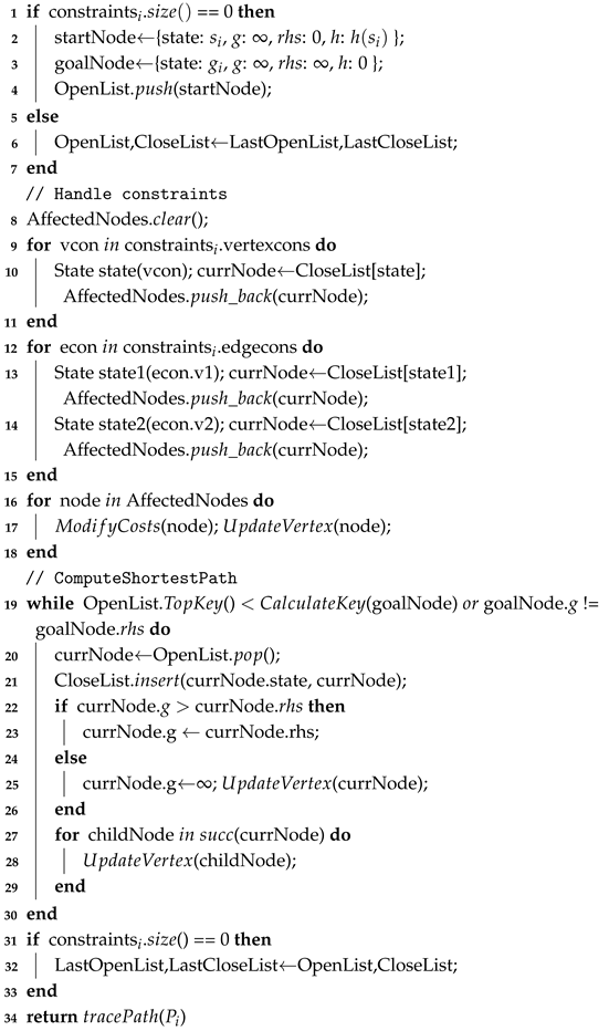 |
Figure 5.
Schematic diagram of the RHCR algorithm computation flow.
The CBS-based RHCR algorithm consists of two main stages: (1) updating the swarm’s initial states and target regions, and (2) generating conflict-free paths using a CBS framework that considers only the first w time steps. In addition, two key improvements are introduced. First, the CBS low-level planner is implemented using the improved LPA* algorithm described in Section 4.1. Second, the time-window parameter w is dynamically adjusted during execution. Since the computational complexity of conflict-free path planning varies across replanning cycles, the corresponding computation time may differ significantly. To address this issue, the time-window parameter is adaptively adjusted whenever the planning time exceeds a predefined threshold. Specifically, the time window is updated according to where , denotes the replanning time and is a scaling factor that typically satisfies . The detailed workflow of RHCR is described in Algorithm 2. Line 1 records the algorithm execution time and updates the initial states and target regions of the swarm. Line 2 constructs the root node, where the low-level planner, denoted by , computes an optimal path that satisfies the specified constraints. Line 3 inserts the root node into OpenList, a priority queue used to represent the constraint tree , and the iterative search process is performed in Lines 4–21. At Line 5, the currently best node is extracted from OpenList, and conflicts within the first w time steps are detected in Line 6. If no conflict is found, the current solution is returned in Line 9. Otherwise, Lines 11–17 identify the earliest conflict in time, generate the corresponding constraints, and construct child nodes. The low-level planner is then invoked to replan paths under the updated constraints, and the resulting child nodes are inserted into OpenList. Finally, Lines 18–20 dynamically adjust the time window w according to the actual computation time.
4.3. MINCO-Based Trajectory Generation Scheme
The set of conflict-free discrete paths generated by the CBS-based RHCR algorithm cannot be executed directly by UAVs. Consequently, an additional trajectory generation and optimization stage is required to produce smooth, dynamically feasible, and collision-free flight trajectories. In trajectory generation and optimization problems, the parameterization of trajectories plays a critical role in determining both the trajectory quality and computational efficiency of the optimization process. Owing to the differential flatness property of quadrotors, motion planning can be performed directly in the flat-output space without considering the full state space, thereby eliminating the differential constraints imposed by the system dynamics [41]. As a result, the position trajectory of a multirotor UAV can be parameterized directly. Unlike conventional polynomial trajectories, Bézier curves, or B-spline curves, the proposed framework adopts the MINCO trajectory representation [34], which features highly sparse parameterization and complete decoupling between temporal and spatial optimization variables. These characteristics make MINCO particularly suitable for efficient trajectory generation and optimization.
As illustrated in Figure 6, let the waypoint vector be denoted by , where and are fixed start and goal waypoints, respectively. The sequence may be obtained from any discrete path generated by RHCR. Let denote the time steps corresponding to waypoints , and let the time duration vector be defined as , where each element represents the duration between two consecutive waypoints. Specifically, , , . A MINCO trajectory is defined such that all M trajectory segments connecting the waypoint sequence are minimum-control trajectories, i.e.,
where is an m-dimensional piecewise polynomial curve consisting of M segments, each of degree . The i-th polynomial segment is expressed as:
where denotes the polynomial coefficient matrix, and is the basis function vector of the polynomial trajectory.
| Algorithm 2: RHCR based on CBS |
Input: , , K; Output: K collision-free paths ; 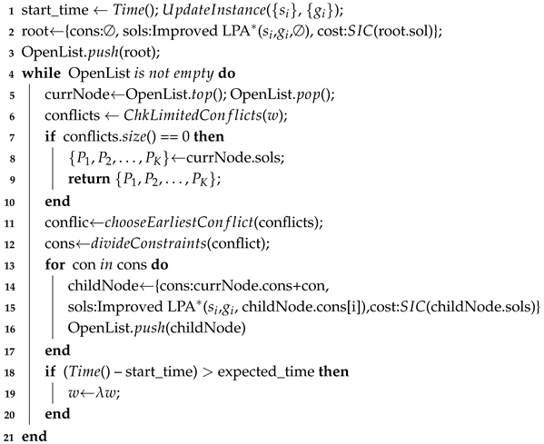 |
Figure 6.
Schematic illustration of MINCO trajectory generation.
The entire MINCO trajectory is parameterized by the waypoint vector and the time duration vector . One of the key properties of MINCO trajectories is that their coefficient matrix can be obtained by solving the linear system , according to Theorem 2 in Reference [34]. It should be noted that and are the notations adopted in Reference [34], and both are constructed directly from and . The coefficient matrix is given by , where . This coefficient matrix is unique and can be computed with linear complexity through PLU decomposition. Furthermore, since the time duration vector is uniformly parameterized, the computational efficiency of MINCO trajectory generation can be further improved by employing a normalized time representation.
4.3.1. Waypoint Selection
During MINCO trajectory generation, the dimension of the linear system is directly related to the computational efficiency of the trajectory generation process. The path generated by RHCR is closely associated with the map resolution and typically consists of a long sequence of discrete waypoints. Since the dimension of the coefficient matrix is directly proportional to the number of trajectory segments, and consequently to the size of the waypoint vector , the dimensionality of is constrained in the proposed framework. As illustrated in Figure 7, the gray waypoints represent the discarded waypoints, whereas the yellow waypoints denote the retained waypoints. A fixed sampling interval is employed for waypoint selection, thereby reducing the number of waypoints and, consequently, the dimension of the coefficient matrix , which improves the computational efficiency of MINCO trajectory generation.
Figure 7.
Schematic illustration of waypoint selection in MINCO trajectory generation.
4.3.2. Local Target Selection
During MINCO trajectory generation, the selection of the start state and target state is of critical importance. Specifically, the complete state information from the 0th-order to the th-order derivatives must be specified for both the start and target states. The full state of the start point can be obtained directly from the VIO system. However, the full state information of the target point may be unavailable in swarm trajectory replanning tasks. Consequently, local target points must be selected along the initially planned global trajectory to recover the corresponding target-state information required for trajectory generation. In general, local targets are selected within a predefined local target selection range. Nevertheless, the local target points assigned to different UAVs are unlikely to be mutually collision-free. However, this does not affect the proposed planning framework because the CBS-based RHCR algorithm considers conflicts only within the first w time steps. Therefore, collisions occurring among local target points beyond the time window do not influence the path-planning process. As illustrated in Figure 8, the local targets of two UAVs may overlap and thus result in a collision. Despite this, the generated paths are only required to remain conflict-free within the first w time steps. Moreover, only the trajectory segment corresponding to the replanning time is actually executed by the UAVs. Here, denotes the local target selection range.
Figure 8.
Illustration of local target selection in MINCO trajectory generation process.
4.4. Time-Windowed Swarm Trajectory Joint Optimization Framework
After a trajectory has been generated using the MINCO framework, further trajectory optimization is required to satisfy specific mission objectives and operational constraints. Let denote the cost function or constraint penalty function, which is assumed to be twice continuously differentiable. The optimization objective of the MINCO trajectory can then be formulated as:
A key property of MINCO trajectories is that the gradients and can be computed with linear complexity from and . Consequently, the MINCO-based swarm trajectory joint optimization framework only requires the design of an appropriate cost function or constraint penalty function and the computation of its corresponding gradients. The gradients of the objective function can then be obtained through gradient propagation, enabling efficient gradient-based optimization of the trajectory.
The proposed MINCO-based swarm trajectory joint optimization framework consists of a smoothness cost, a time cost, and penalty costs arising from dynamic feasibility constraints, obstacle avoidance constraints, and inter-UAV collision avoidance constraints. To enable unconstrained optimization, all dynamic feasibility, obstacle avoidance, and collision avoidance constraints are formulated as soft constraints and incorporated into the objective function in the form of penalty terms. Accordingly, the proposed MINCO-based swarm trajectory joint optimization framework is formulated as:
where , , , and denote the weighting coefficients associated with the respective cost terms. Specifically, represents the smoothness cost, represents the time cost, represents the penalty cost associated with continuous-time constraints, such as dynamic feasibility, collision avoidance, and obstacle avoidance, while represents the cost for enforcing a uniform distribution of sampled constraint points. The waypoint vector and the time duration vector are taken as the optimization decision variables. The design of each cost component is described in detail as follows.
(1) Smoothness cost : is defined as the integral of the squared control input along the MINCO trajectory, which corresponds to the control effort. Specifically,
(2) Time cost : is generally defined as the sum of the durations of the M trajectory segments, i.e.,
However, to eliminate the time constraint , a simple diffeomorphic transformation is adopted, following Reference [34], to convert the constrained variable into the unconstrained variable , i.e.,
(3) Penalty cost associated with continuous-time constraints : The dynamic feasibility constraint , obstacle avoidance constraint , and collision avoidance constraint are all continuous-time constraints , which can be uniformly expressed as:
These continuous-time inequality constraints are incorporated into the objective function as a penalty cost . As illustrated in Figure 9, each MINCO trajectory segment is uniformly sampled along the time dimension, generating constraint points, denoted by . The position of constraint point is given by , and the corresponding constraint is evaluated as , where . For the continuous-time constraint , the penalty cost defined on the MINCO trajectory is formulated as:
where denotes the penalty cost of the i-th trajectory segment. are the weighting coefficients derived from the trapezoidal rule, and represents the penalty incurred when the constraint at the sampling point is violated. The vector is a weighting vector associated with the degree of constraint violation. Specifically, each element of is set to zero when the corresponding constraint is satisfied and takes a positive value when the constraint is violated, thereby characterizing the severity of the violation.
Figure 9.
Illustration of constrained points after sampling the i-th segment of the MINCO trajectory.
In the CBS-based RHCR algorithm, only conflicts occurring within the time window w are considered, while conflicts beyond the time window w are not explicitly addressed. In fact, since the MINCO trajectory segments outside the time window w are not executed, handling their constraint violations is unnecessary. Therefore, within a complete replanning time duration , constraint violations occurring beyond the time window w are ignored. Specifically, for , the corresponding elements of the weighting vector are set to zero, thereby eliminating any penalty associated with constraint violations in this interval.
(3-1) Dynamic feasibility constraints : Based on the maximum velocity and maximum acceleration , the dynamic feasibility constraints can be formulated as:
(3-2) Obstacle avoidance constraint : Let denote the distance between the UAV and an obstacle located at , and let denote the required obstacle-clearance distance. Following Reference [33], when the distance between the UAV and the obstacle, , is smaller than the safety clearance , the obstacle avoidance constraint is defined as
where is the unit vector directed from toward the tangent plane of the obstacle at .
(3-3) Inter-UAV collision avoidance constraint : As illustrated in Figure 10, , , and denote the k-th, -th, and -th UAV trajectories, respectively, where . Assuming that the swarm collision-checking timestamp is , the following relationship holds:
According to Figure 10, the corresponding times of the trajectory segments associated with trajectories and at the collision-checking timestamp are and , respectively.
Figure 10.
Schematic illustration of the computation of inter-UAV collision-avoidance constraints for swarm trajectories.
Let denote the minimum safe separation distance between UAVs. The constraint imposed on the constraint point of trajectory by other trajectories at the timestamp is defined as:
Specifically, the constraint imposed by trajectory is given by:
where
The weighting matrix is defined as:
where the diagonal matrix characterizes the weighted Euclidean distance in different dimensions. Specifically, indicates that the UAV is modeled as a sphere, whereas corresponds to an ellipsoidal UAV model that accounts for the downwash effect.
(4) Uniform distribution cost of sampled constraint points : In the penalty formulation for continuous-time constraints, a non-uniform sampling distribution may cause certain constraint violations to be missed between adjacent sampling points. As a result, all sampled constraint points may appear to satisfy the constraints, while the underlying continuous trajectory may, in fact, violate them. To mitigate this issue, a uniform distribution of constraint points is encouraged by penalizing the variance of the squared distances between adjacent constraint points. For a MINCO trajectory, the total number of constraint points is . The vector of squared distances between adjacent constraint points is defined as:
Accordingly, the uniform distribution cost of the sampled constraint points is defined as:
This cost term penalizes variations in the spacing between adjacent constraint points, thereby promoting a more uniform sampling distribution along the trajectory and reducing the likelihood of undetected constraint violations between neighboring samples.
The computation of the gradients of the smoothness cost , time cost , continuous-time constraint penalty cost , and uniform sampling distribution cost with respect to and , as well as the computation of the gradients of the dynamic feasibility constraint , obstacle avoidance constraint , and inter-UAV collision avoidance constraint with respect to and , can be carried out following the methods presented in References [15,28]. Subsequently, by applying the gradient propagation relationships between , and , provided in Reference [34], the optimization problem associated with the objective function H can be efficiently solved.
4.5. Two-Stage Temporal Coordination Optimization Method
In the proposed MINCO-based swarm trajectory joint optimization framework, a wide range of practical constraints and operational requirements encountered in real-world scenarios have been comprehensively considered. In particular, the optimization methods for obstacle avoidance and inter-UAV collision avoidance in the spatial domain are both highly flexible and computationally efficient. However, time optimization remains a major challenge for swarm motion planning solvers due to its computational complexity. On the one hand, time optimization is highly dependent on the initial values of the time duration vector . In the proposed framework, this issue is largely alleviated by the front-end planner, which generates a time-uniform waypoint sequence and thereby provides a favorable initialization for . On the other hand, the objectives of swarm time optimization are generally either to minimize the overall mission duration or to achieve simultaneous arrival times among all UAVs, both of which are frequently adopted in swarm task execution. The objective of minimizing the overall mission duration has already been addressed in Section 4.4. However, simultaneous arrival has not been adequately handled. To address this issue, a two-stage temporal coordination optimization method is proposed. Since all UAVs in a swarm are treated as equivalent agents, the assignment of individual UAVs to different target regions can be adjusted accordingly. Therefore, in the first stage, a task allocation method oriented toward temporal load balancing is developed to minimize the variance of flight times across all UAVs. This stage also provides a favorable initialization for the subsequent time optimization process. In the second stage, a soft-constrained temporal coordination optimization method is proposed to encourage all UAVs to arrive at their respective destinations as simultaneously as possible.
4.5.1. Task Allocation Method for Temporal Load Balancing
In the first stage, the problem is formulated as an MIQP problem. Let the number of UAVs be K, and define the binary decision variable to indicate whether is assigned to the j-th target region , i.e.,
Let denote the estimated time cost for to reach the j-th target region. It is defined as:
where is the distance precomputed using the A* algorithm, is a velocity scaling factor, and . The expected arrival time is then given by:
Here, represents the average estimated arrival time of all UAVs under a given task assignment and serves as a reference for achieving temporal load balancing across the swarm.
The objective function is designed to minimize the variance of the arrival times. Accordingly, the optimization problem can be formulated as:
subject to:
The optimization variable is the assignment matrix , and the objective is to minimize the variance of the estimated arrival times. The constraints require that each UAV be assigned to exactly one target region and that each target region be assigned to exactly one UAV. The resulting MIQP problem is solved using OR-Tools, Google’s open-source optimization suite. This approach provides efficient task-allocation performance and is capable of handling swarm sizes of up to 1000 UAVs within practical computational time limits.
4.5.2. Time Optimization Based on Soft Constraints
Based on the assignment solution obtained in the first stage, the expected arrival time can be recomputed. In the second stage, the variance of the UAV arrival times is further optimized. To this end, the time cost in the MINCO-based joint swarm trajectory optimization framework is redefined as:
With this modification, the gradients of the time cost are recalculated as and . By incorporating the expected arrival time as a soft constraint into the objective function, the optimization process encourages the flight durations of individual UAVs to converge toward a common value, thereby improving arrival-time simultaneity across the swarm while preserving the flexibility of the trajectory optimization framework.
5. Experiments
The RHCR-Opt algorithm is executed on a computer equipped with an Intel Core i7-8700 CPU running at 3.2 GHz and 16 GB of memory. The software platform consists of a ROS environment based on the Ubuntu operating system. The complete C++ implementation of the project is open-sourced on GitHub at https://github.com/ucas-zihaowang/RHCR-Opt.git, accessed on 10 August 2026. To evaluate the performance of the proposed RHCR-Opt algorithm, we have conducted five experiments, including: (1) performance improvement of CBS through the improved LPA* algorithm, (2) performance analysis of RHCR-Opt, (3) swarm flight in special scenarios, (4) comparison with baseline algorithms, and (5) analysis of the effectiveness of the two-stage temporal coordination optimization. Through these five simulation experiments, we have comprehensively validated the performance improvements achieved by the various components of RHCR-Opt with respect to their corresponding evaluation metrics, confirming that RHCR-Opt maintains high-quality trajectories while simultaneously achieving high computational efficiency.
5.1. Performance Improvement of CBS by Improved LPA*
Compared with A*, the improved LPA* algorithm is more efficient when repeatedly searching for paths under identical spatiotemporal constraints. We employ A* and LPA* as the low-level planners within CBS, respectively, and analyze the performance of CBS (A*) and CBS (LPA*) when solving the same test instances.
5.1.1. Setting
As shown in Figure 11, a map is generated with 20 randomly distributed obstacles of varying sizes. The map resolution is set to 0.1 m, resulting in a grid map of size . We design a test instance involving four agents that cross paths while moving toward each other’s initial positions, with each agent having a radius of 0.25 m. The MAPF problem illustrated in Figure 11 is solved using both CBS (A*) and CBS (LPA*). The high-level planner remains identical to that of the classical CBS algorithm, while A* and the improved LPA* are respectively employed as the low-level planners to search for paths under identical spatiotemporal constraints whenever a conflict is resolved.
Figure 11.
Path planning results in dense obstacle environments using CBS(LPA*). The gray regions represent static obstacles. The solid dark-blue and dark-green circles denote the start and goal positions of the agents, respectively. The four agents move toward their respective goal locations along intersecting routes. The light-green polyline segments represent the agent paths generated by the CBS (LPA*) algorithm.
5.1.2. Results
As shown in Figure 12, the numbers of expanded nodes and computation times of agent 0 and agent 1 are presented for different low-level planners during the high-level iterations of CBS. From the node expansion results in Figure 12a,c, LPA* expands a relatively large number of nodes during the initial planning stage because it needs to process the global consistency of all nodes in the search graph. Except for this initial planning process, the number of expanded nodes remains at a single-digit level, whereas A* consistently expands nodes on the order of hundreds. Correspondingly, as shown in Figure 12b,d, the computation time of LPA* is longer only during the initial planning stage. For all subsequent replanning processes, its computation time is significantly lower than that of A*. It should be noted that when the MAPF problem is extremely simple and CBS requires only a few iterations to resolve conflicts, the improved LPA* does not outperform A*. However, when the MAPF problem becomes moderately complex or the swarm size increases, the improved LPA* exhibits clear advantages over A*. Table 2 presents the performance evaluation results of CBS (A*) and CBS (LPA*) for the problem shown in Figure 11. Compared with CBS (A*), CBS (LPA*) achieves a 73.3% reduction in the number of iterations and an 82.2% reduction in computation time. Therefore, by dynamically maintaining the search graph and flexibly accommodating spatiotemporal constraints, the improved LPA* substantially improves the computational efficiency of CBS when solving MAPF problems in complex environments.
Figure 12.
Node expansions and computational time of CBS under different low-level planners (A* and LPA*).
Table 2.
Performance evaluation metrics of the CBS algorithm under different low-level planners.
5.2. Performance Analysis of RHCR-Opt
To analyze the contribution of each component of RHCR-Opt to the overall performance improvement, we design four algorithmic configurations for the performance analysis experiments: CBS (A*)-Opt, CBS (LPA*)-Opt, CBS (LPA*)-Opt-R, and RHCR (LPA*)-Opt. CBS (A*)-Opt employs A* as the low-level planner within CBS and integrates the MINCO-based swarm trajectory joint optimization framework. In contrast, CBS (LPA*)-Opt adopts LPA* as the low-level planner. Both CBS (A*)-Opt and CBS (LPA*)-Opt perform a one-shot global planning process and do not possess online replanning capability. CBS (LPA*)-Opt-R is the replanning version of CBS (LPA*)-Opt, in which replanning is performed at fixed time intervals. RHCR (LPA*)-Opt, on the other hand, is a swarm trajectory replanning framework based on the RHCR concept, enabling trajectory replanning through rolling-horizon collision resolution.
5.2.1. Setting
As shown in Figure 13, the map size is with a resolution of 0.1 m, and contains 15 cylindrical obstacles of randomly generated sizes. Four UAVs travel from the initial region to the target region along intersecting routes. Each UAV is modeled as a sphere with a radius of 0.25 m, with a maximum velocity of 1 m/s and a maximum acceleration of 6 m/, subject to jerk-based control, i.e., . In addition, the replanning time is set to 2 s, and the local target selection range is set to 3 m. The algorithm performance is analyzed from two perspectives. The first focuses on the performance of CBS in generating conflict-free paths, including the swarm conflict-free path cost, the number of CBS high-level iterations, and the CBS computation time. The second focuses on the performance of the MINCO-based swarm trajectory joint optimization framework, including the flight time cost of swarm trajectories, the control effort cost (i.e., the smoothness cost), and the computation time required for trajectory optimization.
Figure 13.
Flight trajectories of RHCR-Opt under four different algorithm configurations. The gray pillars represent static obstacles. The UAV swarm has successfully flown from the initial swarm region to the target region. The trajectories of individual UAVs are illustrated by curves of different colors.
5.2.2. Results
Figure 13 presents the flight trajectories generated by the four algorithmic configurations for the same test instance, while the detailed performance evaluation metrics are reported in Table 3. As observed from the flight trajectories in Figure 13a,b, the final trajectories generated by CBS (A*)-Opt and CBS (LPA*)-Opt exhibit slight differences, which arise from the different initial paths produced by A* and LPA*, respectively. According to the quantitative results in Table 3, both methods achieve identical path costs. However, CBS (LPA*)-Opt significantly reduces the number of CBS high-level iterations and computation time, with reductions of 67.7% and 90.4%, respectively. In terms of the MINCO-based swarm trajectory joint optimization, CBS (A*)-Opt and CBS (LPA*)-Opt produce nearly identical trajectory time costs and control effort costs, while their trajectory optimization times differ only by a few milliseconds. These results further validate the effectiveness of the improved LPA* in improving the computational efficiency of the overall front-end planning framework, as discussed in Section 5.1. Figure 13c,d illustrate the flight trajectories generated by CBS (LPA*)-Opt-R and RHCR (LPA*)-Opt, both of which perform swarm trajectory replanning at fixed time intervals. The resulting trajectories are largely consistent between the two methods. However, the experimental results in Table 3 indicate that neither CBS (LPA*)-Opt-R nor RHCR (LPA*)-Opt guarantees globally optimal paths or trajectories because of the continuous replanning process. Consequently, both the path cost and trajectory cost are noticeably higher than those of CBS (A*)-Opt and CBS (LPA*)-Opt. Nevertheless, the iterative replanning strategy substantially reduces both the CBS computation time and the trajectory optimization computation time. Figure 14 compares the performance evaluation metrics of CBS (LPA*)-Opt-R and RHCR (LPA*)-Opt throughout the replanning process. Compared with the baseline algorithm CBS (LPA*)-Opt-R, RHCR (LPA*)-Opt achieves significant reductions in the number of CBS high-level iterations, CBS computation time, and MINCO-based swarm trajectory optimization computation time. This improvement is attributed to the fact that RHCR (LPA*)-Opt resolves conflicts only within a finite time window at the CBS high level. Furthermore, Figure 14 more clearly demonstrates that the swarm path cost and swarm trajectory flight time cost remain highly consistent throughout the replanning process, while RHCR (LPA*)-Opt achieves a lower swarm trajectory control effort cost. Therefore, RHCR-Opt substantially improves computational efficiency in both path searching and trajectory optimization while maintaining high trajectory quality. Based on the quantitative results in Table 3, the overall computation time is reduced by approximately 37.5%.
Table 3.
Performance evaluation metrics of RHCR-Opt under four different algorithm configurations.
Figure 14.
Comparison of performance evaluation metrics between RHCR-Opt and baseline algorithms during replanning iterations.
5.3. Swarm Flight in Special Scenarios
Scenarios such as wall-passage traversal and symmetric position exchange are commonly used in swarm flight experiments to evaluate algorithm performance under extreme conditions. We employ the state-of-the-art decentralized planning algorithm Ego-Swarm-v2 [15] as a benchmark and conduct flight tests in both wall-passage traversal and symmetric exchange scenarios under identical algorithmic parameters. As shown in Figure 15, Figure 15a,b present a test scenario in which eight UAVs cross through a wall opening, while Figure 15c,d illustrate a symmetric exchange scenario in which eight UAVs, initially arranged in a circular formation, move toward one another’s initial positions. In the wall-passage traversal scenario shown in Figure 15a,b, Ego-Swarm-v2 [15] does not successfully pass through the wall opening. Instead, as the UAVs approach the opening, the increasing complexity of the swarm trajectories causes several UAVs to choose paths that fly over the wall. This phenomenon reflects a limitation of decentralized planning algorithms such as Ego-Swarm-v2 [15]: when UAVs become densely clustered or operate within narrow spaces, each UAV focuses solely on locally optimal trajectories, which may lead to inferior overall swarm trajectory quality. Consequently, the final flight trajectories generated by RHCR-Opt exhibit higher trajectory quality. Similarly, in the symmetric exchange scenario shown in Figure 15c,d, Ego-Swarm-v2 [15] exhibits frequent hovering behaviors, trajectory distortions, and trajectory backtracking. These phenomena arise from the lack of global coordination during real-time swarm flight. In contrast, RHCR-Opt avoids such issues through its decentralized front-end planning and centralized conflict-resolution mechanism. Therefore, RHCR-Opt generates smoother and more intuitive flight trajectories in challenging scenarios such as wall-passage traversal and symmetric position exchange.
Figure 15.
UAV swarm flight trajectories in special scenarios. The gray walls or gray pillars represent static obstacles. The UAV swarm has successfully flown from the initial swarm region to the target region. The trajectories of individual UAVs are depicted by curves of different colors. (a) Ego-Swarm-v2 [15]. (b) RHCR-Opt. (c) Ego-Swarm-v2 [15]. (d) RHCR-Opt.
5.4. Comparison with Baseline Algorithms
We further conduct large-scale performance comparison experiments between RHCR-Opt and baseline algorithms. Two recent state-of-the-art methods that follow a technical framework similar to that of RHCR-Opt, namely RBP [27] and EDG-TEAM [28], are selected as baseline algorithms. Among them, RBP [27] is employed as a global planning baseline for comparison with RHCR-Opt. Its front-end planner consists of ECBS, a bounded-suboptimal variant of CBS, while its back-end adopts a swarm trajectory joint optimization framework based on Bernstein polynomial trajectories. In contrast, EDG-TEAM [28] is employed as a replanning baseline. Similar to RBP [27], its front-end planner also utilizes ECBS; however, its back-end adopts a MINCO-based swarm trajectory joint optimization framework.
5.4.1. Setting
As shown in Figure 16, the map size is with a resolution of 0.1 m, and six cylindrical obstacles are randomly generated. The UAV radius is set to 0.1 m, with the maximum velocity being 1.7 m/s and the maximum acceleration being 6.2 m/, subject to jerk-based control, i.e., . For replanning tasks, the replanning time is set to 2.0 s, and the local target selection range is set to 6 m. To evaluate performance under different swarm scales, we consider UAVs. For each swarm size, 20 test instances with randomly generated start and goal regions are created. If the computation time of a swarm planning algorithm exceeds 5 s, the corresponding instance is regarded as unsolved. In the front-end ECBS planner used by both RBP [27] and EDG-TEAM [28], the bounded-suboptimality factor is set to 1.0 to ensure that the front-end planners of the baseline methods and RHCR-Opt all maintain optimality. To ensure a fair comparison, the batch size parameter in RBP [27] is set equal to the swarm size, thereby disabling priority-based techniques such as batch processing. Furthermore, when comparing RHCR-Opt with RBP [27], we introduce an additional variant, denoted as RHCR-Opt*. To facilitate a clearer analysis of the performance differences among the various components of the overall framework, RHCR-Opt* replaces the CBS-based RHCR module with an ECBS-based RHCR module while keeping all other modules identical to those of RHCR-Opt.
Figure 16.
Flight trajectories planned by RHCR-Opt for a swarm size of . The gray pillars represent static obstacles, and curves of different colors represent flight trajectories of UAVs.
5.4.2. Results
In a single global planning task, we conduct large-scale batch experiments on RHCR-Opt, RHCR-Opt*, and RBP [27] under different swarm sizes. The corresponding results are presented in Table 4. As shown in Table 4, for problems with different swarm sizes, RBP [27] and RHCR-Opt achieve nearly identical path costs in the front-end planning stage. However, the front-end computation time of RBP [27] is substantially lower than that of RHCR-Opt. This outcome is expected because, in a single global planning task, the CBS-based RHCR framework employs LPA* as the low-level planner, whose node expansion count is considerably higher than that of A*. This characteristic has already been discussed in Section 5.1. Furthermore, RHCR-Opt* adopts an ECBS-based RHCR framework similar to that of RBP [27], and its front-end computation time is also largely comparable to that of RBP [27]. Therefore, the relatively higher front-end computation time of RHCR-Opt in global planning tasks is consistent with expectations. In the back-end optimization stage, the Bernstein polynomial trajectory framework adopted by RBP [27] is theoretically less capable of spatiotemporal trajectory deformation than the MINCO-based framework employed by RHCR-Opt. Consequently, RBP [27] performs noticeably worse than RHCR-Opt in terms of trajectory length, trajectory flight time, and Makespan. It should be noted that Makespan here refers to the maximum trajectory flight time among all UAVs in the swarm. In particular, regarding trajectory flight time and Makespan, RBP [27] relies on fixed time-step settings and essentially lacks the capability to dynamically adjust time duration. Naturally, the longer trajectory flight times and larger Makespan values also result in lower control effort costs for RBP [27] compared with RHCR-Opt. In terms of computational efficiency, RHCR-Opt significantly outperforms RBP [27]. Across all test instances with different swarm sizes, the trajectory optimization time of RHCR-Opt remains within 4 ms to 34 ms and exhibits only a modest approximately linear increase as the swarm size grows. Compared with RBP [27], the computation time is reduced by at least one to two orders of magnitude. Considering the complete planning framework, including both the front-end and back-end stages, RHCR-Opt achieves improvements in success rate across all swarm sizes. Moreover, as the swarm size increases, the overall computation time exhibits a reduction approaching one order of magnitude relative to the baseline method.
Table 4.
Performance evaluation metrics of RHCR-Opt and baseline algorithms in global planning tasks.
In replanning tasks, Figure 16 presents the flight trajectories generated by RHCR-Opt for a swarm size of . Similarly, we conduct large-scale batch experiments to compare RHCR-Opt with the baseline method EDG-TEAM [28] under different swarm sizes in swarm trajectory replanning scenarios. The corresponding results are summarized in Table 5. As shown in Table 5, regarding front-end computation time, when the swarm size is relatively small, or , the replanning task is comparatively simple. Consequently, RHCR-Opt requires slightly more computation time than EDG-TEAM [28] because the initial planning stage of the LPA* low-level planner involves a larger number of node expansions. However, when the swarm size increases to or , the benefits of the proposed improvements to LPA* become increasingly evident, enabling RHCR-Opt to achieve significantly lower front-end computation times than EDG-TEAM [28]. In the back-end optimization stage, the time-window-based swarm trajectory joint optimization framework employed by RHCR-Opt processes fewer conflicts and constraints within each replanning iteration. As a result, RHCR-Opt consistently requires less back-end computation time than EDG-TEAM [28] across all swarm sizes, with the computational advantage becoming more pronounced as the swarm size increases. Moreover, RHCR-Opt achieves superior performance in terms of trajectory length, trajectory flight time, and control effort cost. Overall, RHCR-Opt achieves improvements in success rate over EDG-TEAM [28] for swarm sizes of , , and . When the swarm size is relatively small, or , the larger number of node expansions during the initial execution of LPA* results in a longer overall computation time for RHCR-Opt. However, as the swarm size increases, or , the combined benefits of the front-end and back-end improvements lead to increasingly significant reductions in total computation time, exceeding 23.7% in all cases. For example, when , RHCR-Opt reduces the total computation time by 54 ms. When , the reduction reaches 97 ms.
Table 5.
Performance evaluation metrics of RHCR-Opt and baseline algorithms in replanning tasks.
Based on the above results, RHCR-Opt incurs a certain computational overhead in the front-end planning stage when the swarm size is relatively small, regardless of whether the task involves one-shot global planning or online replanning. However, as the swarm size increases, the computational efficiency of the RHCR-Opt front-end improves significantly. Furthermore, owing to the time-window-based swarm trajectory joint optimization framework employed in the back-end, the computational efficiency of the overall planning process becomes substantially higher. At the same time, RHCR-Opt achieves superior performance in terms of trajectory length, trajectory flight time, and control effort cost. Specifically, the improved LPA* primarily reduces the redundant low-level searches in computationally intensive CBS instances, whereas RHCR mainly decreases the number of conflicts to be resolved and the optimization constraints to be handled during each replanning cycle. Subsequently, the MINCO-based swarm trajectory joint optimization transforms the resulting discrete paths into dynamically feasible trajectories without sacrificing trajectory quality. For small and simple instances, the initialization overhead of LPA* may limit its advantages. However, as the swarm size and conflict density increase, the benefits of search reuse and rolling-horizon processing become increasingly significant.
5.5. Effect of Two-Stage Temporal Coordination Optimization
To address swarm missions that require simultaneous arrival, RHCR-Opt incorporates an additional two-stage temporal coordination optimization method. The effectiveness of the proposed method is evaluated using three metrics: the average flight time, the flight-time range, and the variance of flight times.
5.5.1. Setting
In Figure 17, we design a swarm mission in which all UAVs are required to arrive at a designated target region simultaneously from their initial region. Three different schemes are considered. In Scheme 1, neither the temporal load-balancing-based task assignment method nor the soft-constraint-based temporal optimization method is employed. Instead, each UAV is randomly assigned a target location within the target region. Scheme 2 extends Scheme 1 by incorporating the soft-constraint-based temporal optimization method. Scheme 3 further extends Scheme 2 by additionally introducing the temporal load-balancing-based task assignment method. Under these three schemes, the simultaneous arrival swarm mission illustrated in Figure 17 is executed, and the resulting performance is analyzed and compared.
Figure 17.
Flight trajectories of RHCR-Opt under the two-stage temporal coordination optimization method. The gray pillars represent static obstacles, and curves of different colors represent flight trajectories of UAVs.
5.5.2. Results
Table 6 summarizes the performance evaluation results under different temporal coordination optimization methods. The results clearly indicate that the proposed two-stage temporal coordination optimization method substantially improves the simultaneous arrival performance of the swarm. Specifically, the flight-time range, defined as the time difference between the earliest-arriving UAV and the latest-arriving UAV, decreases from 0.941 s to 0.386 s. In addition, the variance of flight times decreases from 0.164 to 0.027.
Table 6.
Performance evaluation metrics of RHCR-Opt under different temporal coordination schemes.
6. Conclusions
Balancing trajectory quality and computational efficiency in UAV swarm trajectory replanning represents a fundamental challenge, particularly as swarm size grows and operating environments become more densely cluttered. In this paper, we have proposed RHCR-Opt, a CBS-based swarm trajectory replanning framework that addresses this challenge through rolling-horizon collision resolution. The RHCR-Opt framework consists of three layers. The first two layers comprise the CBS-based RHCR framework, while the third layer performs MINCO-based trajectory generation and optimization. Within the RHCR framework, we propose an LPA*-based low-level planner that explicitly considers spatiotemporal constraints and integrates it into CBS. At the high level of CBS, conflicts are resolved using a rolling-horizon collision-resolution concept. After multiple conflict-free paths are generated by RHCR, a MINCO-based trajectory generation scheme is employed, and a time-window-based swarm trajectory joint optimization framework is developed. Furthermore, to satisfy simultaneous arrival requirements in swarm missions, a two-stage temporal coordination optimization method is proposed. All the proposed contributions have undergone comprehensive experimental validation and quantitative analysis. The simulation results demonstrate that, on the proposed benchmark, RHCR-Opt achieves superior trajectory quality and higher computational efficiency compared with state-of-the-art methods. In particular, when the swarm size becomes large, the computational efficiency improvement exceeds 23.7%.
RHCR-Opt also has several practical limitations. Although trajectory execution is decentralized among UAVs, conflict resolution is performed by a designated planning UAV; thus, the framework relies on reliable and sufficiently low-latency communication as well as the availability of that planner. Its real-time advantage may decrease when swarm size, conflict density, or environmental change rate causes the planning time to approach the replanning interval. Moreover, the present validation assumes a static environment and accurate state information, and therefore does not establish robustness against communication loss, perception error, dynamic obstacles, or model mismatch. These conditions define the current applicability of RHCR-Opt and motivate future work on hybrid decentralized coordination and uncertainty-aware replanning.
Author Contributions
Conceptualization, Y.M.; Methodology, Z.W.; Software, Z.L.; Validation, Z.L.; Formal analysis, Y.M. and H.Y.; Investigation, H.Y.; Resources, Q.Z.; Writing—original draft, Z.W.; Visualization, Q.Z.; Supervision, Q.Z.; Project administration, Y.M. and M.Z.; Funding acquisition, Y.M. and M.Z. All authors have read and agreed to the published version of the manuscript.
Funding
This research was funded by Network and Electromagnetic Cross-Domain Collaborative Protection Technology grant number 2023YFC3321404.
Data Availability Statement
The original contributions presented in this study are included in the article. Further inquiries can be directed to the corresponding author.
Conflicts of Interest
The authors declare no conflicts of interest.
References
- Li, J.; Tinka, A.; Kiesel, S.; Durham, J.W.; Kumar, T.K.S.; Koenig, S. Lifelong multi-agent path finding in large-scale warehouses. In AAMAS ’20: Proceedings of the 19th International Conference on Autonomous Agents and MultiAgent Systems; International Foundation for Autonomous Agents and Multiagent Systems: Richland, SC, USA, 2020; pp. 1898–1900. [Google Scholar]
- Lal, R.; Prabhakar, P. Time-optimal multi-quadrotor trajectory planning for pesticide spraying. In Proceedings of the 2021 IEEE International Conference on Robotics and Automation (ICRA), Xi’an, China, 30 May–5 June 2021; pp. 7965–7971. [Google Scholar]
- Tian, Y.; Liu, K.; Ok, K.; Tran, L.; Allen, D.; Roy, N.; How, J.P. Search and rescue under the forest canopy using multiple uavs. Int. J. Rob. Res. 2020, 39, 1201–1221. [Google Scholar] [CrossRef] [Scilit]
- Asghar, A.B.; Sundaram, S.; Smith, S.L. Multirobot persistent monitoring: Minimizing latency and number of robots with recharging constraints. IEEE Trans. Robot. 2025, 41, 236–252. [Google Scholar] [CrossRef] [Scilit]
- Mellinger, D.; Kushleyev, A.; Kumar, V. Mixed-integer quadratic program trajectory generation for heterogeneous quadrotor teams. In Proceedings of the 2012 IEEE International Conference on Robotics and Automation, St. Paul, MN, USA, 14–18 May 2012; pp. 477–483. [Google Scholar]
- Augugliaro, F.; Schoellig, A.P.; D’Andrea, R. Generation of collision-free trajectories for a quadrocopter fleet: A sequential convex programming approach. In Proceedings of the 2012 IEEE/RSJ International Conference on Intelligent Robots and Systems, Algarve, Portugal, 7–12 October 2012; pp. 1917–1922. [Google Scholar]
- Alonso-Mora, J.; Breitenmoser, A.; Rufli, M.; Beardsley, P.; Siegwart, R. Optimal reciprocal collision avoidance for multiple non-holonomic robots. In Distributed Autonomous Robotic Systems: The 10th International Symposium; Springer: Berlin/Heidelberg, Germany, 2013; pp. 203–216. [Google Scholar]
- Xu, G.; Zhu, D.; Cao, J.; Liu, Y.; Yang, J. Shunted collision avoidance for multi-uav motion planning with posture constraints. In Proceedings of the 2023 IEEE International Conference on Robotics and Automation (ICRA), London, UK, 29 May–2 June 2023; pp. 3671–3678. [Google Scholar]
- Qin, J.; Qin, J.; Qiu, J.; Liu, Q.; Li, M.; Ma, Q. SRL-ORCA: A socially aware multi-agent mapless navigation algorithm in complex dynamic scenes. IEEE Robot. Autom. Lett. 2024, 9, 143–150. [Google Scholar] [CrossRef] [Scilit]
- Jiang, Y.; Hu, S.; Damaren, C.; Luo, L.; Liu, B. Trajectory planning with collision avoidance for multiple quadrotor uavs using dmpc. Int. J. Aeronaut. Space Sci. 2023, 24, 1403–1417. [Google Scholar] [CrossRef] [Scilit]
- Scheffe, P.; Pedrosa, M.V.A.; Flaßkamp, K.; Alrifaee, B. Receding horizon control using graph search for multi-agent trajectory planning. IEEE Trans. Control Syst. Technol. 2023, 31, 1092–1105. [Google Scholar] [CrossRef] [Scilit]
- Toumieh, C.; Floreano, D. High-speed motion planning for aerial swarms in unknown and cluttered environments. IEEE Trans. Robot. 2024, 40, 3642–3656. [Google Scholar] [CrossRef] [Scilit]
- Wu, S.; Chen, G.; Shi, M.; Alonso-Mora, J. Decentralized multi-agent trajectory planning in dynamic environments with spatiotemporal occupancy grid maps. In Proceedings of the 2024 IEEE International Conference on Robotics and Automation (ICRA), Yokohama, Japan, 13–17 May 2024; pp. 7208–7214. [Google Scholar]
- Zhou, X.; Zhu, J.; Zhou, H.; Xu, C.; Gao, F. Ego-swarm: A fully autonomous and decentralized quadrotor swarm system in cluttered environments. In Proceedings of the 2021 IEEE International Conference on Robotics and Automation (ICRA), Xi’an, China, 30 May–5 June 2021; pp. 4101–4107. [Google Scholar]
- Zhou, X.; Wang, Z.; Wen, X.; Zhu, J.; Xu, C.; Gao, F. Decentralized spatial-temporal trajectory planning for multicopter swarms. arXiv 2021, arXiv:2106.12481. [Google Scholar]
- Zhou, X.; Wen, X.; Wang, Z.; Gao, Y.; Li, H.; Wang, Q.; Yang, T.; Lu, H.; Cao, Y.; Xu, C.; et al. Swarm of micro flying robots in the wild. Sci. Robot. 2022, 7, eabm5954. [Google Scholar] [CrossRef] [Scilit] [PubMed]
- Tordesillas, J.; How, J.P. Mader: Trajectory planner in multiagent and dynamic environments. IEEE Trans. Robot. 2022, 38, 463–476. [Google Scholar] [CrossRef] [Scilit]
- Kondo, K.; Figueroa, R.; Rached, J.; Tordesillas, J.; Lusk, P.C.; How, J.P. Robust mader: Decentralized multiagent trajectory planner robust to communication delay in dynamic environments. IEEE Robot. Autom. Lett. 2024, 9, 1476–1483. [Google Scholar] [CrossRef] [Scilit]
- Chen, Y.; Guo, M.; Li, Z. Deadlock resolution and recursive feasibility in mpc-based multirobot trajectory generation. IEEE Trans. Autom. Control 2024, 69, 6058–6073. [Google Scholar] [CrossRef] [Scilit]
- Grover, J.; Liu, C.; Sycara, K. Why does symmetry cause deadlocks? IFAC-PapersOnLine 2020, 53, 9746–9753. Available online: https://www.sciencedirect.com/science/article/pii/S2405896320334042 (accessed on 10 August 2026). [CrossRef] [Scilit]
- Stern, R. Multi-agent path finding–an overview. In Proceedings of the Artificial Intelligence: 5th RAAI Summer School, Dolgoprudny, Russia, 4–7 July 2019; pp. 96–115. [Google Scholar]
- Sharon, G.; Stern, R.; Felner, A.; Sturtevant, N.R. Conflict-based search for optimal multi-agent pathfinding. Artif. Intell. 2015, 219, 40–66. Available online: https://www.sciencedirect.com/science/article/pii/S0004370214001386 (accessed on 10 August 2026). [CrossRef] [Scilit]
- Dergachev, S.; Yakovlev, K. Distributed multi-agent navigation based on reciprocal collision avoidance and locally confined multi-agent path finding. In Proceedings of the 2021 IEEE 17th International Conference on Automation Science and Engineering (CASE), Lyon, France, 23–27 August 2021; pp. 1489–1494. [Google Scholar]
- Li, J.; Hoang, T.A.; Lin, E.; Vu, H.L.; Koenig, S. Intersection coordination with priority-based search for autonomous vehicles. In Proceedings of the AAAI Conference on Artificial Intelligence, Washington, DC, USA, 7–14 February 2023; Volume 37, pp. 11578–11585. Available online: https://ojs.aaai.org/index.php/AAAI/article/view/26368 (accessed on 10 August 2026).
- Yan, J.; Li, J. Multi-agent motion planning with bézier curve optimization under kinodynamic constraints. IEEE Robot. Autom. Lett. 2024, 9, 3021–3028. [Google Scholar] [CrossRef] [Scilit]
- Hönig, W.; Preiss, J.A.; Kumar, T.K.S.; Sukhatme, G.S.; Ayanian, N. Trajectory planning for quadrotor swarms. IEEE Trans. Robot. 2018, 34, 856–869. [Google Scholar] [CrossRef] [Scilit]
- Park, J.; Kim, J.; Jang, I.; Kim, H.J. Efficient multi-agent trajectory planning with feasibility guarantee using relative bernstein polynomial. In Proceedings of the 2020 IEEE International Conference on Robotics and Automation (ICRA), Paris, France, 31 May–31 August 2020; pp. 434–440. [Google Scholar]
- Hou, J.; Zhou, X.; Gan, Z.; Gao, F. Enhanced decentralized autonomous aerial robot teams with group planning. IEEE Robot. Autom. Lett. 2022, 7, 9240–9247. [Google Scholar] [CrossRef] [Scilit]
- Koenig, S.; Likhachev, M.; Furcy, D. Lifelong planning a. Artif. Intell. 2004, 155, 93–146. [Google Scholar] [CrossRef] [Scilit]
- Liu, S.; Mohta, K.; Atanasov, N.; Kumar, V. Towards search-based motion planning for micro aerial vehicles. arXiv 2018, arXiv:1810.03071. [Google Scholar]
- Chen, J.; Li, J.; Fan, C.; Williams, B.C. Scalable and safe multi-agent motion planning with nonlinear dynamics and bounded disturbances. In Proceedings of the AAAI Conference on Artificial Intelligence, Virtual Event, 2–9 February 2021; Volume 35, pp. 11237–11245. [Google Scholar] [CrossRef] [Scilit]
- Li, J.; Ran, M.; Xie, L. Efficient trajectory planning for multiple non-holonomic mobile robots via prioritized trajectory optimization. IEEE Robot. Autom. Lett. 2021, 6, 405–412. [Google Scholar] [CrossRef] [Scilit]
- Zhou, X.; Wang, Z.; Ye, H.; Xu, C.; Gao, F. Ego-planner: An esdf-free gradient-based local planner for quadrotors. IEEE Robot. Autom. Lett. 2021, 6, 478–485. [Google Scholar] [CrossRef] [Scilit]
- Wang, Z.; Zhou, X.; Xu, C.; Gao, F. Geometrically constrained trajectory optimization for multicopters. IEEE Trans. Robot. 2022, 38, 3259–3278. [Google Scholar] [CrossRef] [Scilit]
- Tordesillas, J.; How, J.P. Minvo basis: Finding simplexes with minimum volume enclosing polynomial curves. Comput.-Aided Des. 2022, 151, 103341. Available online: https://www.sciencedirect.com/science/article/pii/S0010448522000975 (accessed on 10 August 2026). [CrossRef] [Scilit]
- Honda, K.; Yonetani, R.; Nishimura, M.; Kozuno, T. When to replan? an adaptive replanning strategy for autonomous navigation using deep reinforcement learning. In Proceedings of the 2024 IEEE International Conference on Robotics and Automation (ICRA), Yokohama, Japan, 13–17 May 2024; pp. 6650–6656. [Google Scholar]
- Stern, R.; Sturtevant, N.; Felner, A.; Koenig, S.; Ma, H.; Walker, T.; Li, J.; Atzmon, D.; Cohen, L.; Kumar, T.; et al. Multi-agent pathfinding: Definitions, variants, and benchmarks. Proc. Int. Symp. Comb. Search 2019, 10, 151–158. [Google Scholar] [CrossRef] [Scilit]
- Felner, A.; Stern, R.; Shimony, S.; Boyarski, E.; Goldenberg, M.; Sharon, G.; Sturtevant, N.; Wagner, G.; Surynek, P. Search-based optimal solvers for the multi-agent pathfinding problem: Summary and challenges. Proc. Int. Symp. Comb. Search 2017, 8, 29–37. [Google Scholar] [CrossRef] [Scilit]
- Phillips, M.; Likhachev, M. Sipp: Safe interval path planning for dynamic environments. In Proceedings of the 2011 IEEE International Conference on Robotics and Automation, Shanghai, China, 9–13 May 2011; pp. 5628–5635. [Google Scholar]
- Silver, D. Cooperative pathfinding. In Proceedings of the AAAI Conference on Artificial Intelligence and Interactive Digital Entertainment, Marina Del Rey, CA, USA, 1–3 June 2005; Volume 1, pp. 117–122. Available online: https://ojs.aaai.org/index.php/AIIDE/article/view/18726 (accessed on 10 August 2026).
- Mellinger, D.; Kumar, V. Minimum snap trajectory generation and control for quadrotors. In Proceedings of the 2011 IEEE International Conference on Robotics and Automation, Shanghai, China, 9–13 May 2011; pp. 2520–2525. [Google Scholar]
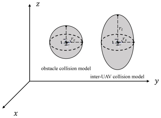
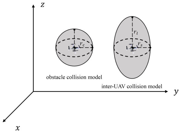
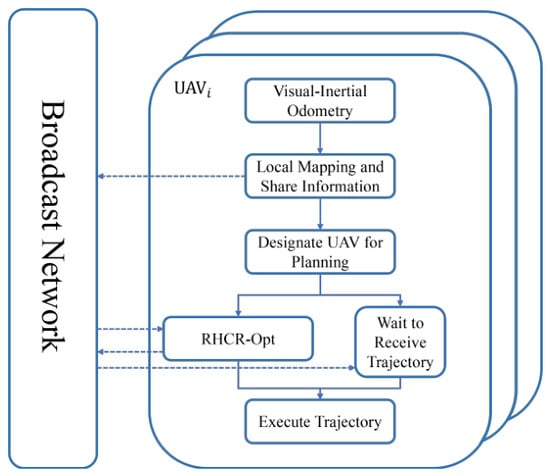
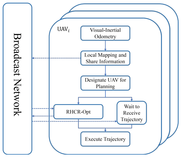
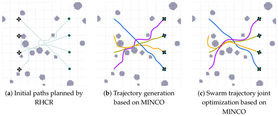
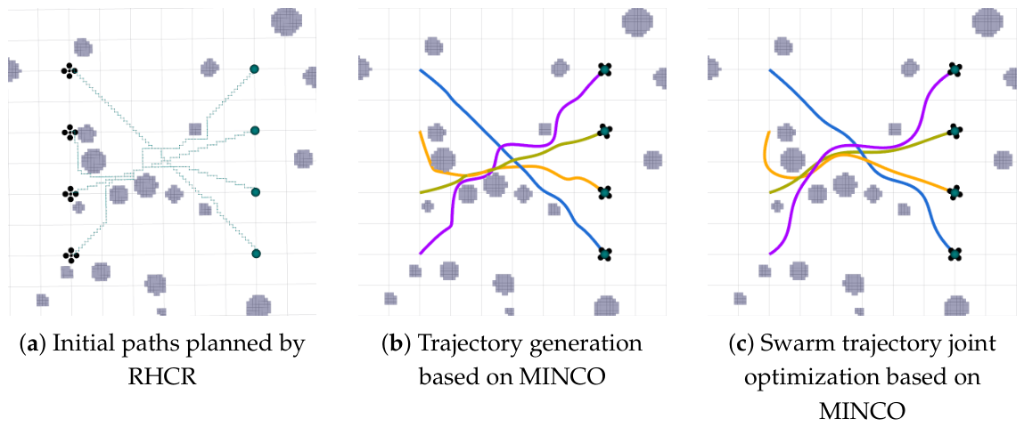
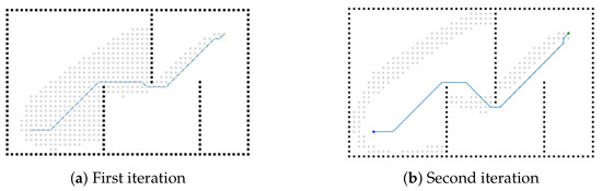
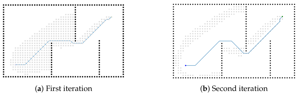
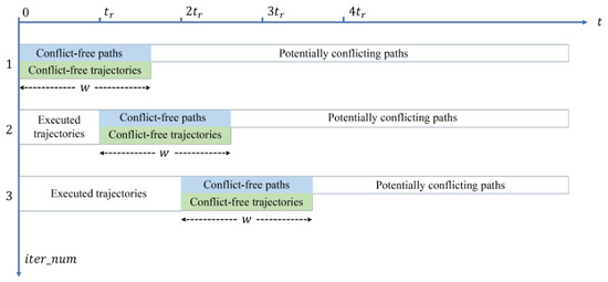
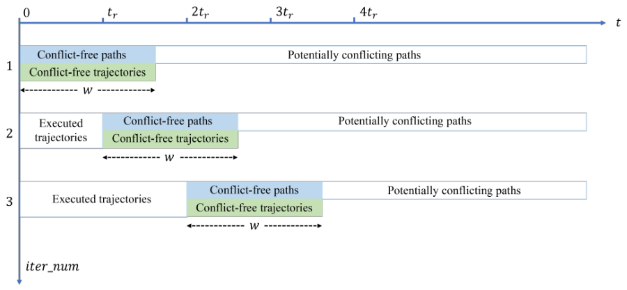
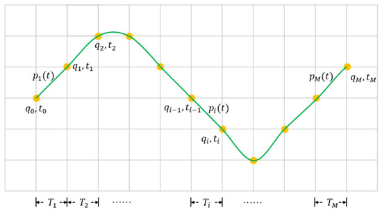
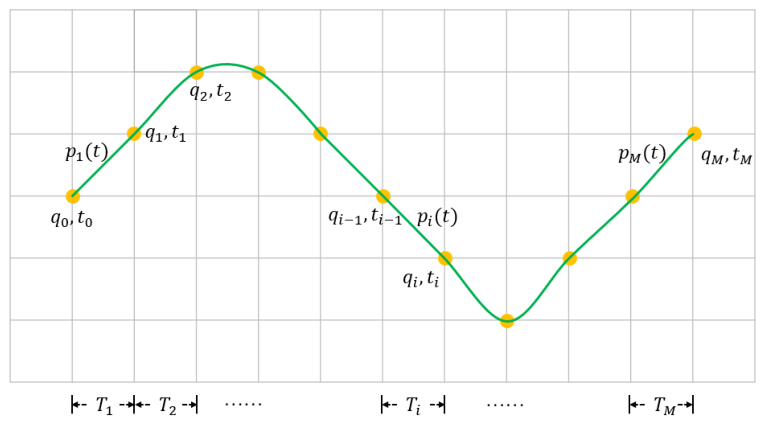
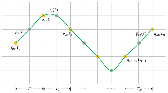
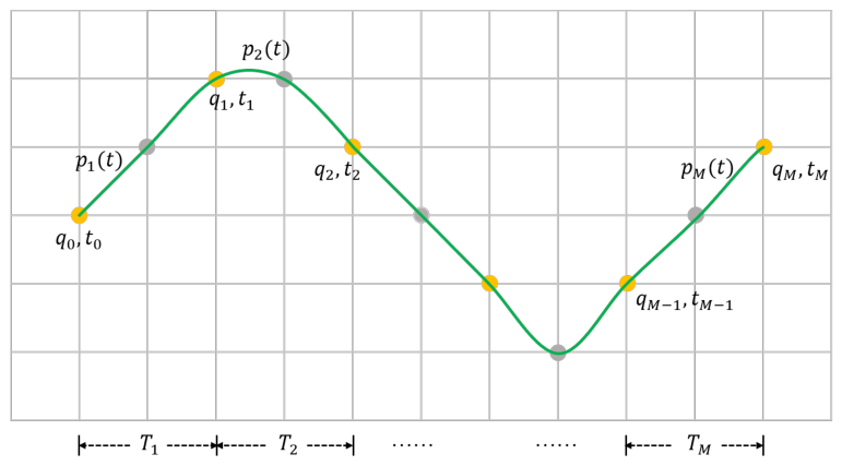
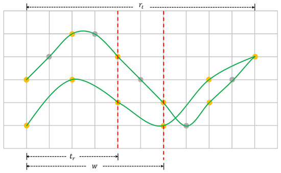
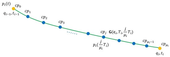
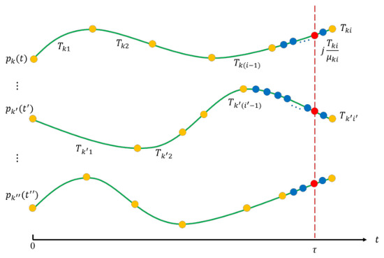
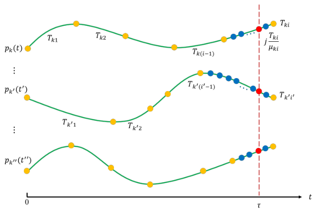
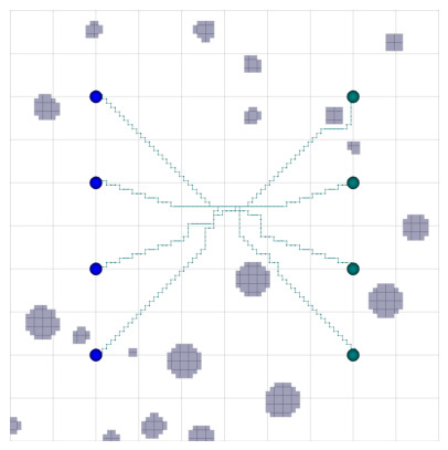
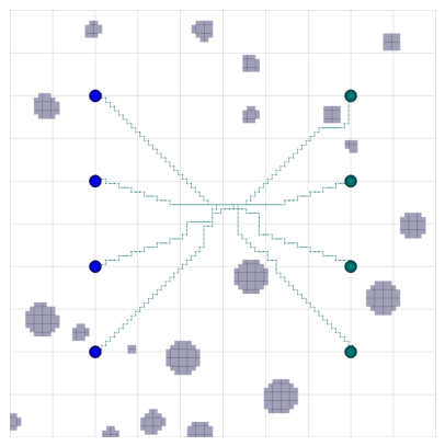
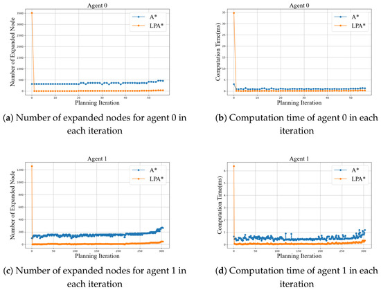
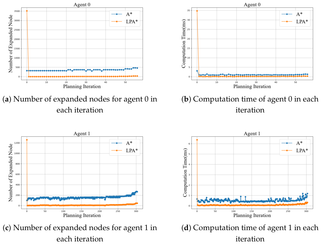
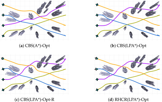
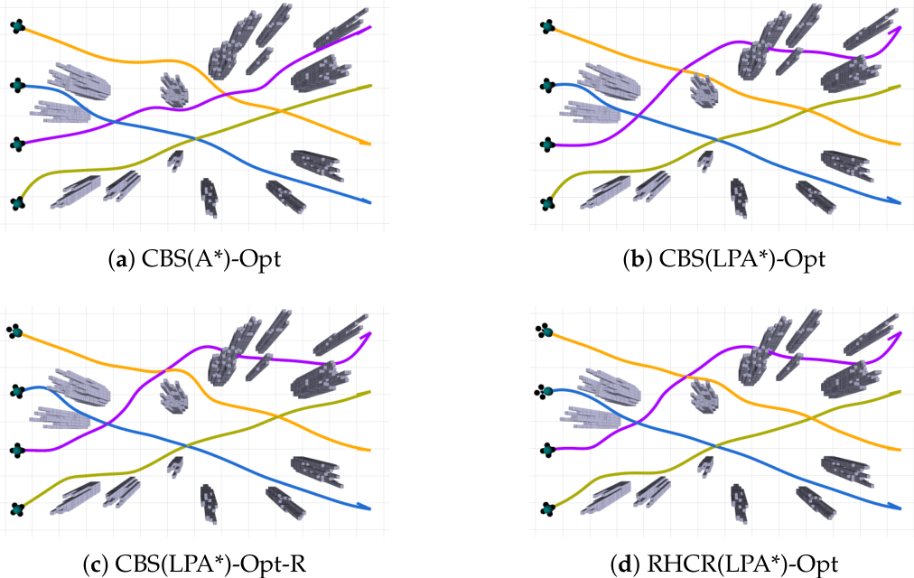
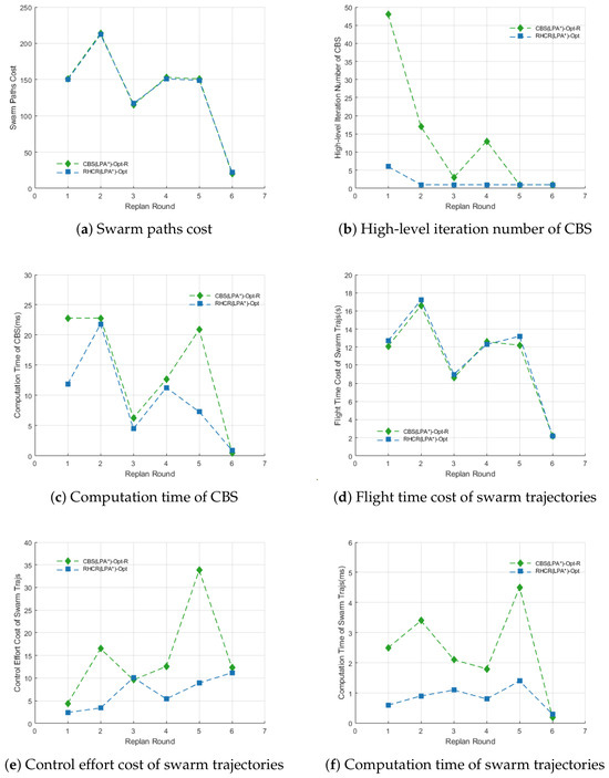
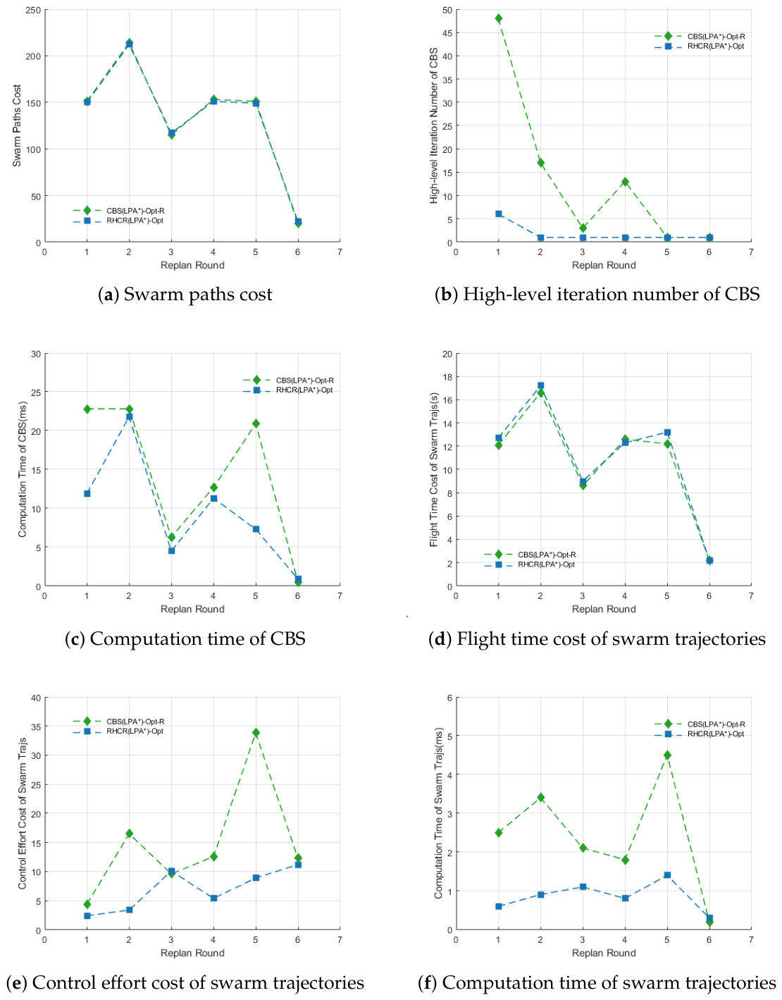
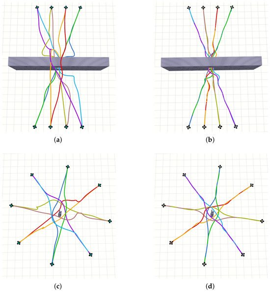
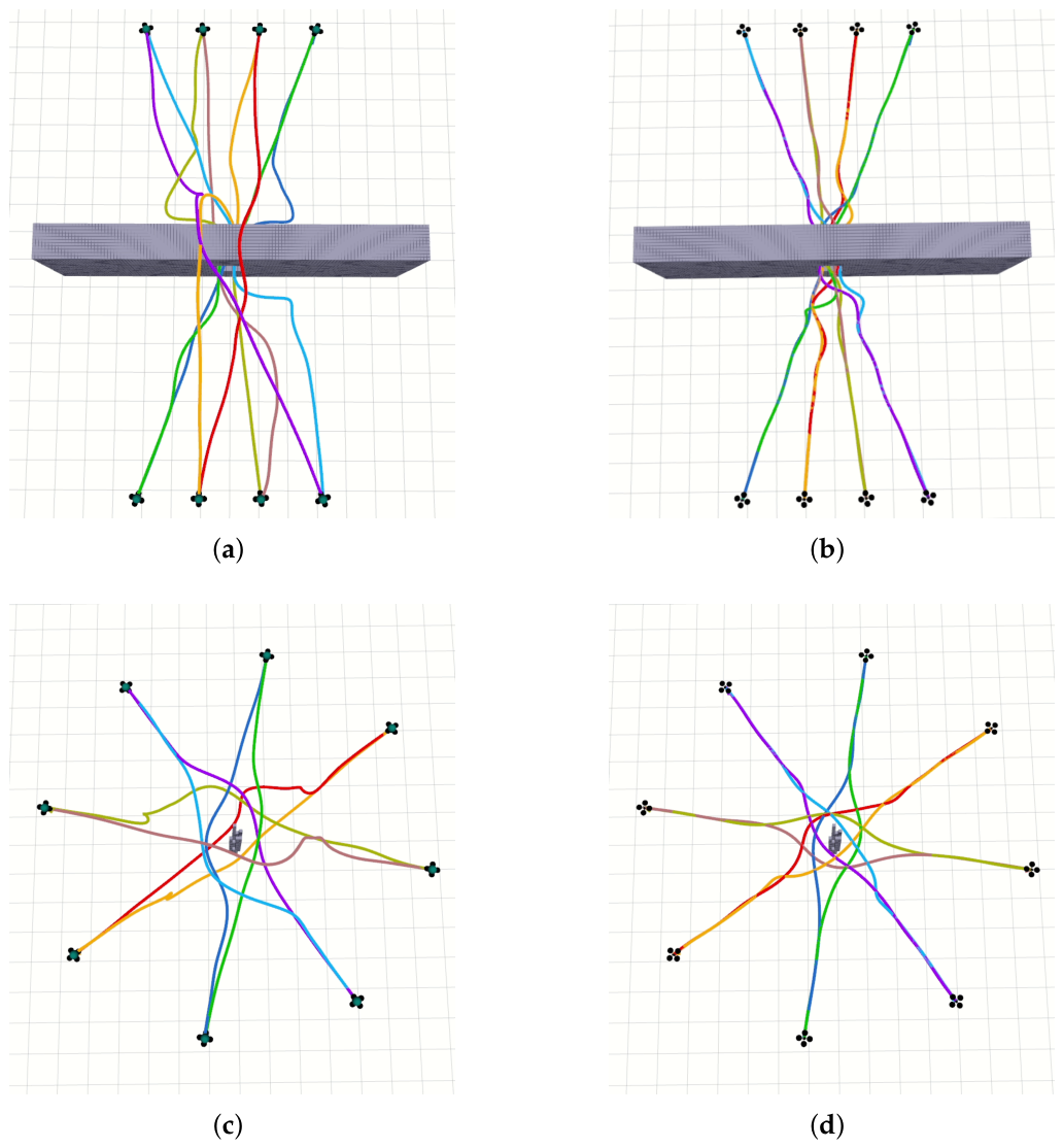
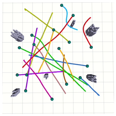
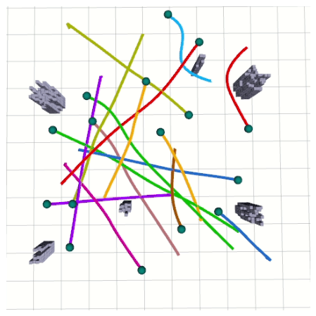
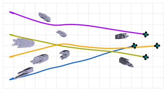
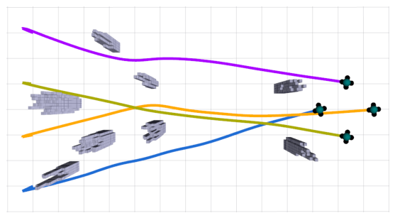

Disclaimer/Publisher’s Note: The statements, opinions and data contained in all publications are solely those of the individual author(s) and contributor(s) and not of MDPI and/or the editor(s). MDPI and/or the editor(s) disclaim responsibility for any injury to people or property resulting from any ideas, methods, instructions or products referred to in the content. |
© 2026 by the authors. Licensee MDPI, Basel, Switzerland. This article is an open access article distributed under the terms and conditions of the Creative Commons Attribution (CC BY) license.