


Highlights
What are the main findings?
- In single-seed training, penalty-dominated reward configurations coincided with exploration collapse in DRL-based drone navigation; controlled multi-seed retraining shows that exploration-noise initialization co-determines this failure mode, while a continuous positive reward gradient remains necessary for convergence.
- Through iterative reward engineering and corrected training mechanics, our PPO-based quadrotor agent achieves 95.0% ± 6.2% navigation success at Stage 0 conditions (2 m targets, no obstacles) and 89.6% ± 6.9% with one obstacle at 4 m, declining to 48.4% ± 10.8% at the full Stage 2 task (7 m, three obstacles); the policy is therefore characterized by a difficulty curve rather than a single figure, with obstacle collisions identified as the dominant failure mode at the hardest setting.
What are the implications of the main findings?
- The documented reward version history provides practical guidance for DRL practitioners on which reward design and training mechanics choices actually govern convergence in continuous control, filling a gap in published methodology on how reward polarity affects continuous control performance.
- A continuous positive shaping gradient is necessary for convergence: removing it yields 0% success across seven seeds. Reward polarity by itself is not the driver, however, since a penalty-heavy reward converges and outperforms the positive-gradient design once the exploration-noise initialization is corrected, so exploration-noise settings should be reported alongside reward weights. The incentive-dominant (positive gradient) reward design principle, supported by the neuroscience literature on reward–punishment asymmetry, suggests that positive-gradient reward design may be more effective than punitive approaches for continuous robotic control tasks similar to the one studied here.
Abstract
This paper presents a systematic reward engineering methodology for training a Proximal Policy Optimization (PPO) quadrotor navigation policy in the Webots simulator, using a hierarchical architecture in which a PID controller handles low-level stabilization and a PPO policy issues velocity commands. We document the complete evolution of a composite ten-term reward function across seven versions (v5 through v11) and retrain the key versions with multiple independent training seeds. The multi-seed study revises the single-seed history: penalty-dominated configurations (v8, v10) fail across all seeds, while the strongest historical version proves seed-sensitive (v11: 32.2 +/− 15.8%). An ablation removing the continuous distance-shaping term from v11 yields 0% success across seven seeds, identifying that term as necessary for convergence. We further isolate a previously hidden co-factor: with the library-default exploration-noise initialization (sigma_0 = 1.0), sampled actions saturate the bounded action space, the exploration variance receives no learning gradient, and curriculum progression deadlocks regardless of reward design; initializing sigma_0 = 0.37 restores gradient flow. With this correction and a deterministic evaluation-gated curriculum, the final configuration is evaluated across the full curriculum rather than at a single operating point: across five independent training seeds under a deterministic protocol, it attains 95.0% ± 6.2% navigation success at Stage 0 conditions (2 m targets, no obstacles), 89.6% ± 6.9% at Stage 1 conditions (4 m, one obstacle), and 48.4% ± 10.8% at Stage 2 conditions (7 m, three obstacles). Reporting this difficulty curve, rather than a single headline value, exposes a substantial generalization gap whose dominant failure mode is obstacle collision (45–52% of episodes at Stage 2). Matched retraining of Soft Actor-Critic and TD3 baselines under identical reward and curriculum conditions yields one completed seed each both baselines show non-monotonic difficulty curves, and at Stage 2 conditions, TD3 (64.0%) exceeds PPO (48.4% ± 10.8%) while SAC (43.0%) falls just below it, whereas at Stage 0, PPO (95.0%) leads both, so the ranking is operating point-dependent on the current single-seed evidence. We conclude that a continuous shaping gradient and the exploration-noise initialization, interacting with the curriculum advancement criterion, determine convergence in continuous control deep reinforcement learning, and that reward polarity by itself does not.
1. Introduction
Autonomous navigation of Unmanned Aerial Vehicles (UAVs) in environments with obstacles remains a challenging problem in robotics, with applications spanning inspection, search-and-rescue, and autonomous logistics [1]. Classical control methods, such as PID controllers, and classical obstacle avoidance techniques, such as potential-field methods [2], can stabilize a drone in hover and avoid nearby obstacles, but they require explicit models of the environment and do not generalize well to dynamic or cluttered scenarios [3]. Deep reinforcement learning (DRL) offers a model-free alternative where the agent learns navigation policies directly from interaction with the environment [4].
This challenge is especially acute for micro-UAVs such as the Bitcraze Crazyflie 2.1, a 27 g open-source quadrotor with approximately seven minutes of flight time and a maximum payload of 15 g. Such platforms cannot carry heavy sensors like LiDAR or depth cameras, limiting the observation space to lightweight inertial and proximity sensors. Furthermore, their limited onboard resources (an STM32F405 at 168 MHz) make running large neural networks in real time infeasible without dedicated hardware acceleration. These platform-specific constraints directly shape the RL system design: the observation space must be compact, the policy network must be small enough for edge deployment, and the control architecture must integrate with existing low-level flight firmware. Addressing these constraints while achieving reliable autonomous navigation is the central engineering challenge of this work.
Among the available DRL algorithms, Proximal Policy Optimization (PPO) has become widely adopted for continuous robotic control due to its training stability, computational efficiency, and tolerance to hyperparameter variation [5]. PPO uses a clipped surrogate objective that constrains policy updates to a trust region, which prevents the destructive large updates that can cause catastrophic failure in systems with sensitive dynamics like quadrotors. Combined with established implementations such as Stable-Baselines3 [6], PPO provides a reliable foundation for UAV control research.
However, even with a good algorithm choice, the design of the reward function remains the most critical and least systematic aspect of DRL for robotic navigation. Small changes in reward component weights or penalty magnitudes can drastically alter the learned behavior, shifting the policy from functional navigation to complete failure. Despite this sensitivity, most published works present only the final reward function without documenting the design iterations that led to it. This gap leaves practitioners without practical guidance on how to tune rewards for their own systems.
In this paper, we address this gap by presenting the complete iterative reward engineering process for training a PPO-based quadrotor navigation policy. We document seven versions of our reward function (v5 through v11), including the failures, and analyze the relationship between reward design choices and resulting agent behavior. The single-seed history initially suggested that the balance between positive incentives and negative penalties, what we call reward polarity, was the critically overlooked factor. The controlled multi-seed experiments reported here revise that reading. What the reward must supply is a continuous positive shaping gradient toward the goal, whose removal causes complete failure across every seed; penalty magnitude is not by itself decisive, since a penalty-heavy reward converges and outperforms the forgiving, positive-gradient design once the exploration-noise initialization and the curriculum advancement criterion are corrected.
The objectives and scope of this study are stated explicitly. Purpose: To document and quantify how reward design and training mechanics jointly determine convergence of a DRL navigation policy for a nano-quadrotor, and to characterize the resulting policy’s performance across the full range of task difficulty rather than at a single operating point. Goals: (i) Evaluate a documented sequence of reward formulations under a multi-seed protocol; (ii) isolate, through controlled experiments, which factors (shaping gradient, penalty magnitudes, exploration-noise initialization, curriculum gating) causally determine convergence; and (iii) benchmark the resulting pipeline against SAC and TD3 on the same task under matched conditions. Scope delimitation: All experiments are conducted in the Webots simulator with a Crazyflie-class model, static obstacles, and full state observability; real-flight validation, moving obstacles, and camera-based sensing are outside the present scope and are identified as future work.
The contributions of this paper are: (1) a documented iterative reward engineering methodology for DRL-based UAV navigation, now supported by quantitative multi-seed retraining of the key reward versions; (2) a hierarchical PID + PPO control architecture validated in Webots with a three-stage curriculum; (3) a controlled identification of exploration-noise initialization as a co-determinant of convergence, experimentally separable from reward design; (4) an ablation establishing the continuous distance-shaping term as necessary for convergence; and (5) a matched-conditions comparison protocol against SAC and TD3 baselines on the same task, environment, and reward, together with the first completed TD3 seed evaluated under that protocol.
The rest of this paper is organized as follows. Section 2 reviews related work. Section 3 describes the system design, environment parameters, and reward function methodology. Section 4 presents experimental results across all versions. Section 5 discusses the findings, and Section 6 concludes the paper.
2. Related Works
2.1. DRL for UAV Navigation
DRL has been applied extensively to UAV control problems in recent years [3]. The most commonly used algorithms for continuous control are PPO [5], Soft Actor-Critic (SAC), Deep Deterministic Policy Gradient (DDPG) [7], and Twin Delayed DDPG (TD3). PPO is particularly suited for robotics applications because of its clipped objective function, which provides stable training even with noisy sensor inputs and nonlinear dynamics [5,6]. Several works have demonstrated PPO-based navigation for drones in simulation environments, typically using some a combination of distance-to-goal rewards, collision penalties, and stability terms.
Within the drone-specific DRL literature, several recent studies are particularly relevant. Lee et al. [3] provided a comprehensive survey of deep learning methods for drone navigation autonomy, categorizing approaches by sensor modality, control level, and simulation platform. Koch et al. [8] demonstrated PPO-based attitude control for quadrotors, showing that RL can match or exceed hand-tuned PID controllers for low-level stabilization. Pham et al. [9] applied DRL to UAV obstacle avoidance using depth images, achieving collision-free navigation but requiring onboard cameras that add significant weight and power draw. Song et al. [10] developed the Flightmare simulator specifically for high-throughput drone RL training, demonstrating that simulation speed directly impacts the feasibility of training. In contrast to these works, our approach uses a sensor-only observation space (IMU and proximity sensors, no cameras) designed for deployment on resource-constrained micro-UAVs like the Crazyflie 2.1, and focuses specifically on the reward engineering methodology rather than novel network architectures or sensor modalities.
2.2. Reward Shaping in DRL
The theory of potential-based reward shaping [11] established that certain classes of supplementary rewards can speed up learning without changing the optimal policy. However, in practice, reward design in deep reinforcement learning for robotics goes beyond simply adding a potential function. When designing reward–penalty functions, multiple competing objectives must be balanced. These objectives include target achievement, flight stability, energy efficiency, and obstacle avoidance. Each of these objectives has its own corresponding reward or penalty. The sensitivity of deep reinforcement learning agents to reward magnitude and sign has been observed in numerous contexts [4,12], yet studies documenting the iterative tuning of rewards for drone navigation are scarce in the scientific literature. Some recent studies have highlighted the ongoing challenges of manually engineering rewards in deep reinforcement learning for drone navigation. Chen and Xuan [13] proposed an inverse deep reinforcement learning framework for learning an unknown reward function from expert demonstrations. Sheng et al. [14] studied deep reinforcement learning strategies for autonomous UAV navigation in highly dynamic, high-density environments. This highlights the crucial role of sophisticated and iterative reward design in achieving robust quadcopter performance.
2.3. Simulation Environments for Drone RL
Training DRL policies requires millions of environment interactions, making simulation essential. Popular platforms include AirSim [15], Gazebo [16], Flightmare [10], and Webots [17]. AirSim provides photorealistic rendering but can be slow for non-visual tasks. Gazebo is widely used with ROS integration but has a complex setup. Webots offers a good balance between physics fidelity and computational efficiency, with a native Python API and built-in support for various robotic platforms including quadrotors [17,18]. We selected Webots for its lightweight simulation loop, which allows running millions of training steps within reasonable time frames.
2.4. Curriculum Learning for Robotic Tasks
Curriculum learning [19] structures the training process by gradually increasing task difficulty. For drone navigation, this typically means starting with short-distance targets and no obstacles, then progressively adding longer distances and more obstacles. This strategy helps the agent build basic navigation competence before facing complex scenarios, and prevents early training from being dominated by sparse terminal rewards that provide no learning signal.
2.5. Hierarchical Control Architectures
A common approach in DRL-based drone control is to separate the control into two levels. The high-level DRL policy outputs velocity or waypoint commands, while a low-level PID controller handles the attitude stabilization and motor commands [3]. This simplifies the DRL task by abstracting away the complex nonlinear dynamics of the quadrotor and allows the DRL agent to focus on navigation decision-making.
Recent work (2023–2025) sharpens the context for this study. End-to-end DRL navigation with collision avoidance in unknown environments has been demonstrated at increasing scale [20], including high-density dynamic scenes [14] and perception-constrained settings addressed with guided exploration [21]. On resource-limited platforms comparable to ours, depth-based obstacle avoidance has been deployed fully onboard nano-UAVs [22]. Algorithmically, PPO variants with representation enhancement [23] and TD3 variants with prioritized replay [24]—building on distributed prioritized replay foundations for scaling deep RL [25]—report strong path-planning results, while sim-to-real transfer at the state of the art has reached champion-level drone racing with policies trained largely in simulation [26,27]. Across this literature, however, the reward function is typically presented as a finished artifact and exploration-noise settings are rarely reported at all; the systematic documentation of the reward engineering process, and the isolation of exploration-noise initialization as a co-determinant of convergence, are the gaps this paper addresses.
3. Materials and Methods
3.1. Drone Platform and System Architecture
The target drone platform is the Bitcraze Crazyflie 2.1 (Bitcraze AB, Malmö, Sweden), a 27 g open-source nano-quadrotor widely used in UAV research due to its small size, low cost, and extensible firmware [28]. The Crazyflie is equipped with a BMI088 6-axis IMU (Bosch Sensortec, Reutlingen, Germany) (accelerometer and gyroscope), a BMP388 barometric pressure sensor for altitude estimation, and supports up to four time-of-flight proximity sensors via expansion decks, providing distance measurements up to 2 m in the cardinal directions. The platform’s maximum flight time is approximately seven minutes on a 250 mAh LiPo battery, and its maximum payload capacity is 15 g. These constraints, particularly the limited payload and short flight time, motivated several key design decisions in this work: (1) the observation space uses only IMU and proximity data rather than camera imagery, keeping the sensor suite lightweight; (2) the policy network was deliberately kept small (two hidden layers of 64 units, the Stable-Baselines3 (v2.9.0) default, verified from the saved checkpoints) to enable future onboard deployment; and (3) a fixed-point FPGA toolchain was validated on a separate and much smaller network as preliminary work (Section 5.4). The inference latency of the navigation policy itself is estimated analytically rather than measured, and no timing claim for that policy is made here.
In simulation, the Crazyflie is modeled using Webots’ built-in quadrotor model with four brushless DC motors, each providing up to 14.5 g of thrust. The Webots model includes rotor drag, motor response dynamics, and gravitational effects, providing sufficient fidelity for policy training while maintaining the simulation speed required for reinforcement learning (the 32 ms timestep allows for the completion of 20 million training steps in approximately 42 h). The simulated sensor suite mirrors the physical platform: an IMU providing roll, pitch, and yaw at each timestep, a GPS module for position feedback (analogous to an optical flow deck on the real Crazyflie), and four distance sensors with a 2 m detection range positioned at 0, 90, 180, and 270 degrees around the drone body.
The system uses a two-level hierarchical control architecture implemented in the Webots robotics simulator [17]. At the high level, a PPO agent [5] receives a 20-dimensional observation vector and outputs 4-dimensional continuous velocity commands. At the low level, a PID controller converts these velocity commands into individual motor speeds through attitude control and motor mixing. Figure 1 summarizes the resulting pipeline.
Figure 1.
System architecture: hierarchical PID + PPO control with curriculum learning.
The observation space S consists of 20 continuous values: goal vector (3D), attitude angles (3D), linear velocity (3D), angular velocity (3D), altitude (1D), distance to target (1D), normalized progress (1D), four proximity sensor readings (4D), and current speed magnitude (1D). All inputs are normalized to prevent gradient saturation [29]. The action space A is a 4-dimensional continuous vector: forward/backward velocity Vx, lateral velocity Vy, vertical velocity Vz, and Yaw_rate, each in the range [−1, 1], which the environment scales to physical units (max 1.5 m/s translational, 1.0 rad/s yaw).
3.2. PID Baseline and Motor Mixing
In detail, the control law is a cascaded PID structure executed at the 32 ms simulation step. Altitude channel: the altitude error, the vertical speed, gains , and the integral term clipped to [−2, 2] for anti-windup; the commanded collective is T = + with = 55 rad/s. Horizontal position hold maps position error to desired tilt: = clip( − , −0.3, 0.3) and = −clip( − , −0.3, 0.3) with (, ) = (0.5, 2.0). Attitude stabilization is a PD law on the IMU angles and gyro rates: = ( − ) − p and with , plus yaw rate damping with .
Motor mixing follows the standard X-configuration: ; ; ; each clipped to [0, 600] rad/s. With these gains, the platform reaches hover with a measured settling time of 3.10 s, mean altitude error of 9.49 cm (std 4.85 cm, max 31.6 cm), and mean horizontal drift of 1.42 cm (max 4.13 cm) over a 37 s hold—the baseline stability on which the learned velocity command policy operates.
Before DRL training, a classical PD controller was implemented to achieve stable hover and validate the simulation environment. The base hover velocity is derived analytically from the drone mass and thrust coefficient, as shown in Equation (1):
Individual motor speeds are then computed using standard quadrotor mixing equations that combine collective thrust with differential pitch, roll, and yaw commands.
3.3. PPO Training Configuration
The PPO agent was implemented using Stable-Baselines3 [6] with an MlpPolicy consisting of two hidden layers of 64 units each for both the actor and the critic (the library default, verified from the saved checkpoints; approximately 11,000 trainable parameters in total). Table 1 lists all training hyperparameters. The historical versions (v5 through v11) were each trained once, with a budget of up to 20 million timesteps for v11 (approximately 42 h on an NVIDIA RTX-class GPU, comprising roughly 129,964 episodes). The multi-seed experiments introduced in this revision (Section 4.6, Section 4.7, Section 4.8 and Section 4.9) train every configuration for 5 million steps per independent seed, with the final configuration receiving an additional 3 million fine-tuning steps at Stage 2, for a total budget of 8 million steps per seed; the matched algorithm baselines of Section 4.8 use the same 8 million-step budget. The multi-seed experiments introduced in this revision (Section 4.6, Section 4.7 and Section 4.8) train every configuration for 5 million steps per independent seed, with the final configuration receiving an additional 3 million fine-tuning steps at Stage 2. In these experiments, the run seed is applied to the Python (v4.14.5) and NumPy (v2.5.2) random-number generators and to the PPO constructor, and the Gaussian policy’s initial log standard deviation is set to −1.0 (sigma_0 approximately 0.37) and verified programmatically at model construction (Section 4.7).
Table 1.
PPO training hyperparameters and configurations.
3.4. Curriculum Learning Strategy
Training followed a three-stage curriculum with automatic advancement based on evaluation success rate. Stage 0 uses 2 m targets with no obstacles. Stage 1 increases to 4 m targets with one obstacle placed between the drone and the target. Stage 2 uses 7 m targets with three obstacles distributed along the path. In the historical versions (v5–v12), advancement required a 30% success rate over a rolling window of stochastic training episodes. Because success measured under exploration-noise systematically underestimates the deterministic policy (Section 4.7), the final configuration replaces this criterion with a periodic deterministic evaluation: at most every 100,000 steps (after a per-stage minimum episode count), 20 episodes are executed with the deterministic policy, and the stage advances when the success rate reaches 60% (Stage 0) or 50% (Stage 1); a fallback budget of 2 million steps per stage guarantees progression. Mid-training evaluation shares the single Webots environment with training; consistency is preserved by resetting the environment and re-synchronizing the learner’s cached observation after each evaluation. This progression ensures the agent learns basic flight before facing obstacles.
Target positions are generated at random angles around the drone to prevent directional bias:
where and d is the stage distance with 10% jitter. Obstacles are placed along the drone-to-target vector at random fractions with lateral offsets, ensuring they are always relevant to the navigation path.
3.5. Environment Parameters and Evaluation Metrics
The small Crazyflie drone was run inside Webots with a step time of 32 ms. We designed the simulation area as a 20 m square ranging from −10 to +10 m, and we put the termination boundary at ±9.5 m so the drone would not fly out. The obstacles were cylinders about 20 cm in radius, placed along the line to the target at fixed fractions with random side shifts of ±1.5 m.
Regarding the evaluation criteria, we defined them as follows: Success means the drone reaches a distance of less than 70 cm from the target and remains in that area for at least three steps (cumulative, not consecutive). We chose 70 cm because it allows for natural deviation during hovering and noise in the assessment. These three steps are relatively short (approximately 0.1 s); Section 4.10 re-reports the headline result under progressively stricter consecutive-dwell requirements up to 1.0 s. Where a single proportion is at issue, we report 95% Wilson confidence intervals (Section 4.10), while results across multiple independent training seeds are reported as the mean ± standard deviation across seeds. Table 2 use the same cumulative in-zone definition of success as this section. Crucially, every reported success rate is accompanied by the curriculum stage at which it was measured, since the stage determines both the obstacle layout and the target distance (2 m/4 m/7 m). An earlier version of our evaluation harness constructed the environment at Stage 0 without overriding the target distance, so results later described as Stage 2 measurements were in fact Stage 0 measurements; all numbers in this revision were regenerated with the stage set explicitly and recorded in every output file.
Table 2.
Complete reward component weights for version 11.
As for navigation efficiency, we defined it based on the percentage of useful progress towards the target compared to the total distance traveled by the drone (Equation (4)). The difference from the old method is that this does not produce falsely high scores if the drone does not reach the target at all.
where is the initial Euclidean distance from the drone to the target, is the remaining distance to the target at the end of the episode, and is the total trajectory length. The metric is bounded to the interval , where 1.0 represents an ideal straight-line trajectory that reaches the target with no unnecessary motion, while lower values indicate reduced navigation efficiency due to detours, oscillatory behavior, or incomplete progress toward the goal. Unlike the previous straight-line-to-path-length ratio, this formulation incorporates the remaining distance to the goal, ensuring that failed episodes cannot achieve artificially high efficiency scores despite making insufficient progress toward the target.
The obstacle collision rate was the percentage of episodes that ended due to the sensor reading being less than 30 cm, and policy deviation was the average deviation in the distribution of actions during the evaluation. The episode ends in six cases: reaching the goal, falling to the ground (height less than 5 cm), excessive tilt (roll or pitch greater than approximately 29 degrees), hitting the obstacle, going outside the boundary, or completing the 300 steps.
3.6. Reward Function Design
Designing the reward function is the most important part of the entire process. The reward at each step was the sum of ten items (Equation (5)). We experimented with dozens of combinations and observed that the weights and the plus or minus sign (+) were far more important than the items themselves.
Each item has its role: the Survival item provides a small reward to encourage the drone to keep flying; the Progress item encourages approaching the target; the Altitude item penalizes incorrect altitude; the Stability item reduces tilt; and the Efficiency item encourages lower speed. There are also penalties for obstacles and boundaries, a bonus for hovering near the target, and a penalty for retreating after approaching.
In Table 2, we list the weights for version v11 for documentation purposes, but the final version we used in the results (4.7–4.8) includes further modifications to the weights and new restrictions.
Terminal rewards are applied only once at the end of the episode, while other rewards are calculated at each subsequent timestep. For clarification, we rely on several dynamic state variables to compute the reward components summarized in Table 2. We denote the current Euclidean distance to the target as (m), the distance at the episode start as (m), and the closest distance achieved so far as (m).
The Progress term relies on the improvement in the closest distance, , defined as:
For obstacle and boundary avoidance, we define normalized proximity metrics and that scale linearly as the drone approaches a threshold:
To discourage the agent from moving away from a previously reached waypoint, we apply an abandonment penalty using , which represents the distance retreated beyond a 1.0 m threshold:
Finally, continuous distance shaping uses the fraction of the initial distance covered, , while the efficiency penalty utilizes a maximum speed threshold of m/s:
3.7. Iterative Reward Engineering Process
Our work from version 1 to 4 focused solely on building the fundamentals: setting up the environment, configuring the PID controller, implementing the Gymnasium wrapper [30], and confirming that the entire pipeline was functioning correctly. These versions were all about building the basics (sensor integration, motor mixing, loop management), and we never delved into systematic reward design.
After confirming that everything was working and the training was stable, we began the real work with version 5. From this point on, we had a clear and structured cycle: (1) We monitor the agent’s behavior using records and metrics. (2) We try to understand the root cause of the problem by analyzing the reward items. (3) We adjust the weights or add a new item. (4) We train and evaluate. (5) We compare the results with previous versions.
We repeated this cycle seven times (from version 5 to version 11), each time building upon the data and observations from the previous version.
Important note: All these experiments were single-seed training, but the evaluation was multi-layered. After receiving very valuable feedback from reviewers focusing on the importance of “not being random” in the results (because one result is not enough), we spent more than 15 days and nights working continuously testing, developing, and modifying, and this is exactly what we will explain in detail in the following sections.
The overall training procedure is summarized in Algorithm 1:
| Algorithm 1: Curriculum-based PPO training with iterative reward engineering. |
|
4. Results
All experiments use the following scenario. The arena is a 20 × 20 m bounded workspace (soft boundary penalties beginning 1.5 m inside the +/−9.5 m edges). Episodes last at most 300 steps of 32 ms (9.6 s). At each reset, the drone starts from hover near the arena center and a target is sampled at a random angle at the stage’s nominal distance: Stage 0 = 2 m with no obstacles; Stage 1 = 4 m with one obstacle; Stage 2 = 7 m with three obstacles placed between start and target. The 20-D observation comprises inertial attitude and rates, position and velocity from the simulator state, the target vector, and Multiranger-class proximity readings with 2.0 m range, consistent with small-form-factor detect-and-avoid sensor evaluations for sUAS [31]; the 4-D action is a velocity/yaw rate command passed to the PID layer. Success, terminations, and metrics are as defined in Section 3.5. Qualitatively, this places the method among end-to-end velocity command DRL policies [20,21,23] rather than planner-hybrid pipelines [32]; the quantitative in-environment comparison against SAC and TD3 appears in Section 4.8.
In the following sections, we will present the results of our work, which is divided into two phases. The first phase consists of initial trials with a single seed and multiple evaluations, while the second phase focuses on multiple seeds and progress from the second stage.
4.1. Version History and Key Changes
Figure 2 visualizes these historical single-seed results, which are superseded by the multi-seed retraining of Section 4.6.
Figure 2.
Historical single-seed navigation success by reward version (v5–v11). Gray bars represent the early designs, dark bars the punitive configurations, and blue bars the final positive-gradient strategy; the dashed line at 50% marks the predefined target threshold. Each bar is a single training run and is superseded by the multi-seed values of Table 3 and Figure 3.
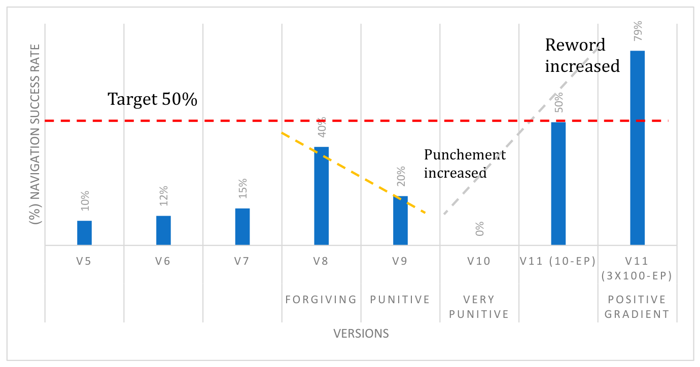
Figure 3.
Multi-seed results (mean +/− SD across independent training seeds): (a) navigation success by reward configuration, including the v11 distance-shaping ablation; (b) algorithm comparison under identical environment, task, and reward conditions. The dashed line marks the 50% target.
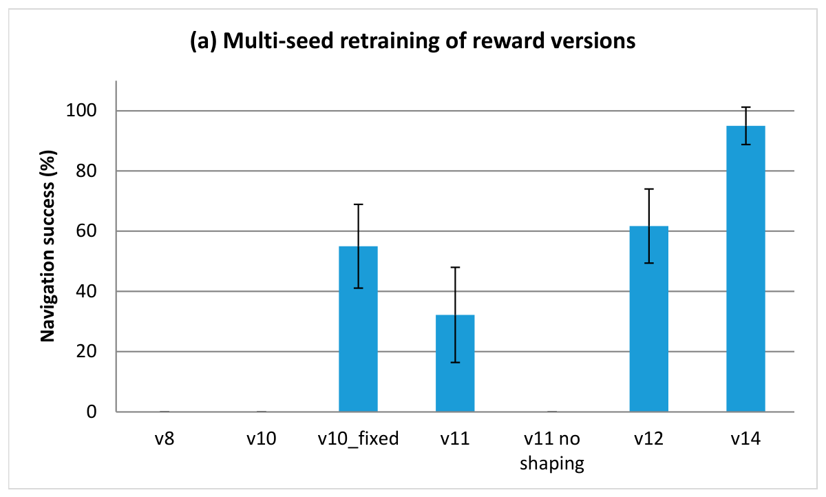
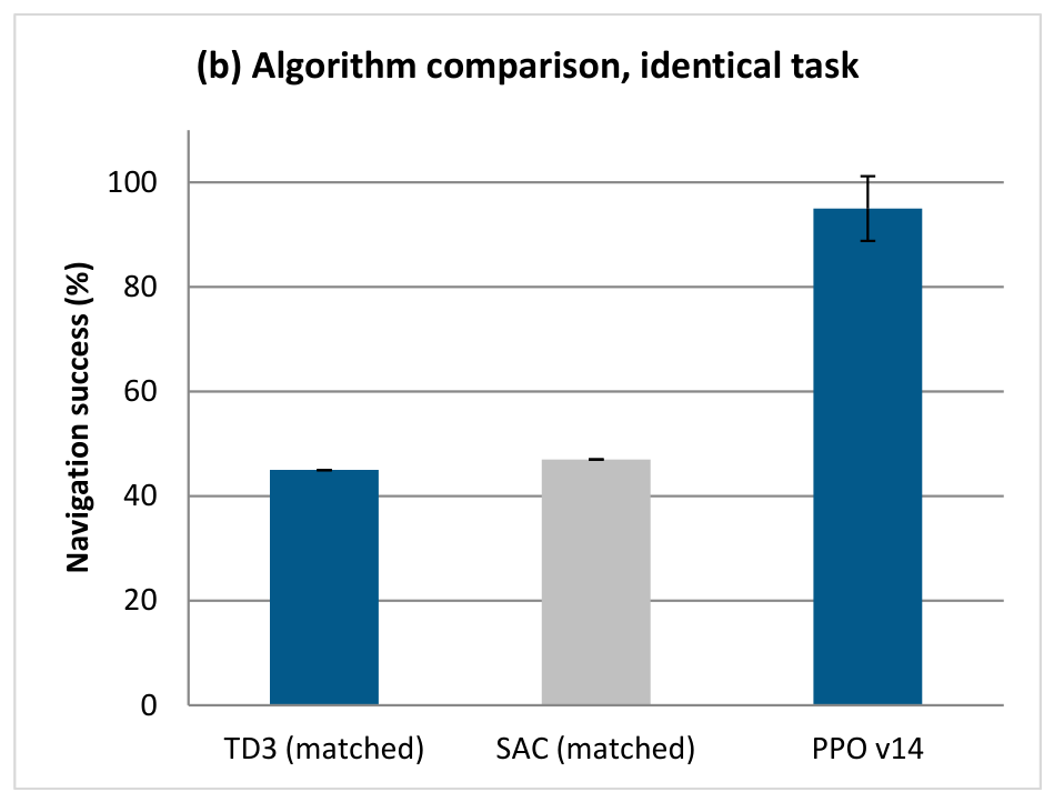
Table 3.
Multi-seed retraining of key reward configurations, evaluated deterministically at Stage 0 conditions (2 m targets, no obstacles). Values are mean +/− standard deviation across independent training seeds; failure percentages are mean episode shares. These are the operating points that the evaluation harness defect described in Section 3.5 had previously mislabeled as Stage 2 measurements; the corrected Stage 2 values, and all three operating points together, appear in Section 4.11.
4.2. Penalty-Dominated Regression: v8 to v10
Version 8 achieved the best performance to that point (40%) with a forgiving design. Increasing punishment in v9 and v10 produced progressive collapse: v9 dropped to 5–20%, and v10 reached complete failure (0% success). The agent converged to a no-movement policy, as evidenced by deeply negative evaluation returns and stalled learning.
4.3. The Recovery: Version 11
The pattern from v8 through v10 was clear: every increase in punishment produced worse results. This led us to reverse the strategy entirely for v11, adopting an incentive-dominant (positive gradient) reward strategy. The key changes were:
- (a)
- Survival reward increased from 0.1 back to 0.3, restoring the exploration incentive.
- (b)
- Crash penalty reduced from −200 to −50, a middle ground between v8 and v9.
- (c)
- Timeout penalty was completely removed, since penalizing the agent for surviving the full episode contradicts the survival reward.
- (d)
- Abandonment penalty softened from −15 to −8 with the trigger relaxed from 0.5 m to 1.0 m.
- (e)
- A new continuous distance-shaping reward was added:
Version 11 was trained for 20 million steps (approximately 42 h, 129,964 episodes). The policy standard deviation converged to 0.228, the lowest across all versions, indicating confident, well-learned actions. The agent advanced through all three curriculum stages and reached Stage 2 (7 m targets, three obstacles).
4.4. Multi-Seed Evaluation of the v11 Best Checkpoint (Evaluation Seeds Only)
In version 11, the evaluation results showed the best checkpoint across three evaluation seeds, each with 100 episodes, achieving a success rate of 79.0 ± 1.7% and a path efficiency of 84.2 ± 2.5%. This was an obstacle-free trial at Stage 0 conditions, exceeding all predefined acceptance criteria (Table 4). In contrast, the baseline based solely on the PID system achieved a 0% success rate under the same conditions, highlighting the necessity of a DRL component. Because both columns of Table 4 are measured at Stage 0 conditions, they should be read together with the full difficulty curve presented later in Section 4.11.
Table 4.
Evaluation results versus predefined objectives: best historical checkpoint of version 11 (mean ± standard deviation across 300 evaluation episodes, three evaluation seeds) and the final configuration of Section 4.7 (mean ± standard deviation across five independent training seeds, deterministic protocol). Both columns are measured at Stage 0 conditions (2 m targets, no obstacles); the corresponding Stage 1 and Stage 2 values for the final configuration are 89.6 ± 6.9% and 48.4 ± 10.8% (see Section 4.11). The obstacle collision rate is counted only on direct contact and is necessarily zero at Stage 0, where no obstacles are present; terminations caused by tilt are recorded separately.
4.5. Cross-Version Comparison
Table 5 places the historical single-seed outcomes of Section 4.1, Section 4.2, Section 4.3 and Section 4.4 alongside the multi-seed retraining introduced in Section 4.6, and the comparison is instructive. Three historical readings do not survive reseeding: v8’s 40% collapses to 0.0% across four seeds; v11’s best checkpoint 79.0% corresponds to a per-training seed mean of 32.2 +/− 15.8%; and the ranking of v11 above the corrected punitive configuration v10-fixed (55.0 +/− 13.9%) reverses. One reading is confirmed: v10 fails across every seed. With inter-seed standard deviations of 12–16 percentage points, differences in that order between versions in the single-seed history are indistinguishable from initialization variance.
Table 5.
Cross-version comparison: historical single-seed results versus multi-seed retraining (deterministic evaluation at Stage 0 conditions, 2 m targets, and no obstacles; see Section 4.6 and Table 6 for all three stages). The divergence between the two columns quantifies seed sensitivity; single-seed entries are observational.
The strongest configurations under the multi-seed protocol are those that combine the continuous shaping gradient with bounded ancillary income and corrected training mechanics: v12 (61.7 +/− 12.3%) and the final configuration (95.0 ± 6.2%), both at Stage 0 conditions.
4.6. Multi-Seed Retraining of Key Reward Versions and Ablation
In response to the seed-sensitivity concern, we retrained the key reward versions with multiple independent training seeds (3–7 seeds per configuration; each seed governs the network initialization, the action-sampling stream, and the environment randomization). Every seed’s final policy was evaluated with the deterministic post hoc protocol of Section 3.5; the values reported in Table 6 are those measured at Stage 0 conditions (2 m targets, no obstacles), and the corresponding Stage 1 and Stage 2 values appear in Section 4.11. Table 6 reports mean +/− standard deviation across training seeds, and Figure 3a visualizes the comparison.
Table 6.
This table summarizes the seven reward versions together with their observed single-seed performance (historical training runs).
The multi-seed results materially revise the single-seed history of Table 6. The forgiving v8 configuration, whose single documented run reached 40%, fails across all four retrained seeds (0.0%), dominated by attitude instability. The punitive v10 fails across all five seeds, as before. The corrected punitive configuration v10-fixed reaches 55.0 +/− 13.9%, whereas v11, whose single best checkpoint produced the previous headline result, averages 32.2 +/− 15.8% across six seeds. Two conclusions follow. First, inter-seed variance is large (standard deviations of 12–16 percentage points), confirming that single-seed comparisons between reward versions are unreliable; the historical version ranking of Section 4.1 should therefore be read as observational. Second, the earlier ranking of v11 above the corrected punitive configuration does not survive the multi-seed protocol.
To isolate the contribution of the distance-shaping term, we additionally trained an ablated variant, v11-no-shaping, identical to v11 except for the removal of the continuous distance-shaping reward of Equation (11). It achieves 0% success across seven independent seeds, with policies predominantly crashing or drifting out of bounds. The continuous positive gradient is therefore necessary for convergence in this task. This supports the positive-gradient element of our original claim while decoupling it from penalty magnitudes: the v11 improvement was driven primarily by the added shaping gradient rather than by penalty softening alone.
4.7. Exploration-Noise Correction and the Final Configuration
The v12 configuration combines the corrected punitive penalty structure of v10-fixed with v11’s distance-shaping and adds boundedness constraints on the hover income: an episodic cap of 40% of the success bonus and a multiplicative obstacle clearance throttle. Together, these guarantee that completing the task strictly dominates loitering near the target for every policy. Across three independent seeds, v12 reaches 61.7 +/− 12.3%. Its training logs, however, exposed a hidden pathology: the policy’s exploration standard deviation remained at 0.95–1.03 for the entire five million steps (verified from the saved checkpoints of all three runs), 96% of training episodes ended in noise-induced attitude crashes at a mean length of roughly 60 steps, the stochastic training success rate was pinned near 3%, and the curriculum never advanced past Stage 0. The very same checkpoints, evaluated deterministically, scored 49.5–71.5% on the Stage 0 sub-task. The mechanism is the interaction of the default noise initialization (sigma_0 = 1.0) with the bounded action space: roughly one third of sampled actions saturate the clipping boundary, so the log-probability used by the policy gradient refers to actions that were never executed, corrupting the gradient with respect to both the action mean and the noise parameter itself. The final configuration therefore applies four corrections at once: (i) the initial log standard deviation is set to −1.0 (sigma_0 approximately 0.37) and verified at model construction; (ii) the stochastic 30% training success gate is replaced by the periodic deterministic evaluation gate of Section 3.4; (iii) the run seed is passed to the PPO constructor in addition to the Python and NumPy generators; and (iv) each seed receives a further three million Stage 2 fine-tuning steps. Section 4.9 tests correction (i) in isolation.
With these corrections, the exploration standard deviation anneals monotonically (0.368 to 0.258 by five million steps, reaching approximately 0.23 by the end of the Stage 2 fine-tuning phase), the curriculum completes all three stages, and the final policies are evaluated across the whole curriculum. Across five independent seeds, they reach 95.0% ± 6.2% success at Stage 0 conditions (2 m targets, no obstacles) and 89.6% ± 6.9% at Stage 1 conditions (4 m, one obstacle); at Stage 2 conditions (7 m, three obstacles), success falls to 48.4% ± 10.8%, with obstacle collisions accounting for 45–52% of episodes and attitude instability for under 3%. (see Section 4.11) reports the full curve for every configuration, and Figure 4 summarizes the final configuration outcome. Because the reward function is identical to v12, the improvement over v12 at matched conditions is attributable to the training mechanics corrections as a group; Section 4.9 tests the noise initialization factor in isolation. The complete reward specification and parameter bounds for this final configuration are detailed in Table 7.
Figure 4.
Final configuration results across five independent training seeds under the deterministic protocol: (a) mean termination breakdown at Stage 0 conditions(obstacle collision and out-of-bounds rates are zero); (b) achieved metrics versus predefined targets at Stage 0 conditions; (c) per-seed success at each of the three curriculum stages. Error bars denote standard deviation across training seeds. Panels (a,b) characterize the Stage 0 operating point only; the Stage 1 and Stage 2 values are those of panel (c) and Table 10.
Table 7.
Complete reward specification of the final configuration (identical to v12; used unchanged by the runs producing the headline result). Notation: d = distance to target (m); = initial distance; = closest approach so far; v = speed; = environment maximum speed; = target altitude; phi, theta = roll and pitch; s = normalized proximity reading in [0, 1]; c = minimum s over all sensors; B = success bonus (3000).
4.8. Comparison with SAC and TD3 Baselines
To address algorithm specificity, we trained Soft Actor-Critic (SAC) and TD3 agents in the same environment and on the same task with multiple independent seeds. During this revision, we established that those runs were not conducted under conditions matched to the final PPO configuration: they used the environment’s default v11 reward rather than the v12 reward used by the PPO pipeline, retained the earlier stochastic curriculum gate rather than the deterministic gate, and were allocated a different step budget. A comparison across differing reward functions cannot isolate the effect of the algorithm, so we withdraw the earlier baseline numbers rather than report them. Matched retraining—identical v12 reward, identical deterministic curriculum gate, identical eight-million-step budget (5 M steps plus 3 M Stage 2 fine-tuning steps)—was completed for TD3 and SAC (one seed each to date). Under the deterministic curriculum gate, the TD3 run advanced from Stage 0 to Stage 2 after only 322,000 steps and consequently spent 95,348 of its 99,018 training episodes (96.3%) at Stage 2 conditions. The deterministic post hoc evaluation of this run (100 episodes per stage; Table 8) gives a markedly non-monotonic curve: 45.0% at Stage 0, 93.0% at Stage 1, and 64.0% at Stage 2 (mean episodic return 2001.9, 3600.0, and 3084.3 respectively)—the opposite pattern from every reward version and PPO result in this paper, all of which decline monotonically with difficulty (see Section 4.11). The termination breakdown localizes the cause: at Stage 0, the dominant termination is attitude instability rather than any obstacle-related failure (Stage 0 has no obstacles), consistent with a policy that, having received only 2689 of its 99,018 training episodes under near-target, obstacle-free conditions, may have specialized around the long-approach deceleration profile demanded by Stage 2 and lost precision at very short range. This is a second, independent illustration of the curriculum-speed effect noted throughout this paper: how quickly a run passes through easier stages shapes what the final policy is competent at, for better (extensive Stage 2 practice) and for worse (possible loss of easy-task competence), simultaneously. A single seed is not sufficient to establish this pattern as general to TD3 rather than a property of this particular run, and we treat it as a preliminary observation pending further seeds. SAC under the same matched protocol reaches 47.0% at Stage 0, 80.0% at Stage 1, and 43.0% at Stage 2 (single seed); like TD3, its curve is non-monotonic, peaking at Stage 1, though its Stage 2 value falls below both TD3 and PPO. We do not presuppose the algorithmic ranking: off-policy methods are frequently more sample-efficient than PPO in continuous control, and at Stage 2, specifically, the single-seed TD3 run (64.0%) exceeds PPO (48.4% ± 10.8%), while the single-seed SAC run (43.0%) falls just below it; at Stage 0, by contrast, PPO (95.0%) is well ahead of both baselines (TD3 45.0%, SAC 47.0%). The ranking therefore depends on the operating point, and no single algorithm dominates across the full difficulty range on the evidence of one seed per baseline. Table 9 presents the statistical comparison of Stage 2 success rates between the different configurations using pairwise Welch tests.
Table 8.
Algorithm comparison under matched reward, curriculum, and step budget conditions, at all three curriculum stages (100 deterministic episodes per stage). TD3 and SAC each reflect a single completed seed under the matched protocol (TD3: run td3_v12reward_seed1009). PPO values are the Table 10 final configuration figures (n = 5 seeds), reproduced here for direct comparison.
Table 9.
Pairwise Welch tests on Stage 2 success (Table 10), Holm-corrected across the family, with Hedges g effect sizes. v8, v10, and the v11-no-shaping ablation are zero-variance across all seeds and are excluded from pairwise testing. SAC and TD3 are excluded from pairwise testing because each currently has a single matched seed (Section 4.8), precluding a variance estimate. Comparisons surviving Holm correction (p < 0.05): v10-fixed vs. v11, v10-fixed vs. v14, v11 vs. v14, v12 vs. v14.
4.9. Single-Factor Test of the Noise Initialization Effect
Because the final configuration differs from v12 in several ways simultaneously (Section 4.7), we ran a single-factor variant that is exactly v12—same reward, same original stochastic curriculum gate, five million steps, no fine-tuning—changing only the exploration-noise initialization from sigma_0 = 1.0 to sigma_0 = 0.37. The per-run seed is additionally passed to the PPO constructor, repairing a seeding defect in the historical v12 runs that is required for any valid multi-seed comparison. Across three seeds, this variant reached 3.0% ± 1.5% deterministic success at Stage 2 conditions (4.5%, 1.5%, and 3.5% for seeds 42, 123, and 43; 200 episodes each), and the training logs show that all three runs remained at Stage 0 for the entire five million steps: the stochastic 30% gate never fired, exactly as it failed to fire for the historical v12 runs.
This result refutes the simplest reading of our own hypothesis, and we report it as such. Correcting the noise initialization in isolation does not reproduce the final configuration’s performance; it does not even match v12’s own Stage 2 result of 12.3% ± 12.3% obtained under sigma_0 = 1.0. The training logs localize the reason: with the stochastic gate retained, no run escaped Stage 0, so all three policies were evaluated at 7 m with three obstacles having been trained only at 2 m without obstacles. The correct conclusion is an interaction rather than a main effect. Reduced exploration-noise is necessary for the training signal to become informative, but without a curriculum gate able to act on that signal, the policy never reaches the conditions it is later asked to solve; conversely, a deterministic gate cannot rescue a policy whose rollouts are destroyed by noise. Neither component is sufficient alone, which is why the final configuration changes both. The initialization contrast underlying this test—the default sigma_0 = 1.0 shared by v8–v12 versus the corrected sigma_0 = 0.37—is shown in Figure 5.
Figure 5.
Exploration-noise initialization across reward versions: the library-default initial policy standard deviation (sigma_0 = 1.0 for v8–v12) and the final policy standard deviation reached at the end of training, by version. The final configuration’s corrected initialization (sigma_0 = 0.37) is shown as the sigma-ablation bar. This complements Figure 6a; the final sigma value is omitted for the sigma-ablation run, which never left Stage 0 and did not produce a converged policy.
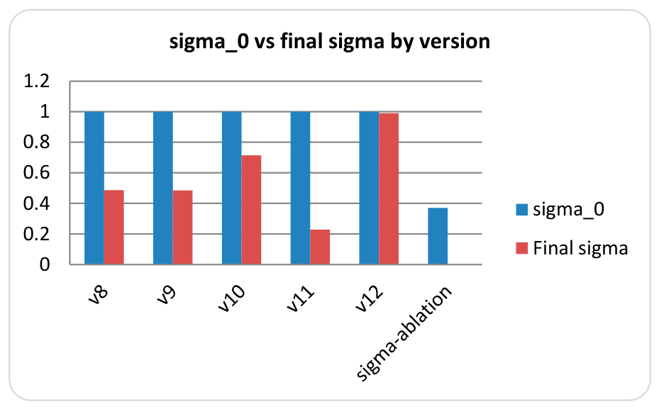
Figure 6.
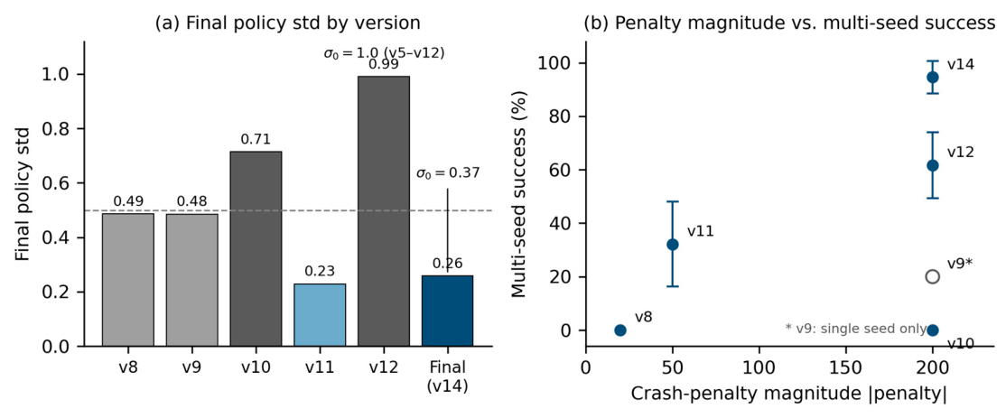
Exploration and polarity analysis revisited: (a) final policy standard deviation by version, annotated with its initialization sigma_0 (the horizontal grey dashed line at 0.5 denotes the convergence threshold; v10 and v12 exhibit two distinct failure signatures); (b) crash penalty magnitude versus multi-seed navigation success. The inverse relationship suggested by the single-seed history does not persist under multi-seed evaluation (the asterisk * and hollow marker for v9 indicate a single-seed evaluation.
4.10. Success Criterion Sensitivity and Robustness Under Perturbations
Success criterion sensitivity. To address the concern that a dwell of roughly 0.1 s could reward a fast fly-through, we re-evaluated all five final configuration seeds with target-reached termination disabled, recording each episode’s longest consecutive in-zone streak (200 episodes per seed, Stage 2 conditions). Averaged across seeds, success under progressively stricter criteria was 40.3% at three consecutive steps (0.10 s), 39.4% at ten steps (0.32 s), 37.9% at sixteen steps (0.51 s), and 30.5% at thirty-one steps (1.0 s), with Wilson 95% intervals reported per seed in the supplementary data. Requiring a five-fold longer dwell therefore costs roughly ten percentage points, and the strongest seed retains 43.5% at a full second. Figure 7 plots this curve. The baseline of this protocol (40.3% at the three-step criterion) is lower than the 48.4% ± 10.8% of Table 10 because target-reached termination is disabled here, so an episode does not end on first arrival in the goal zone and may subsequently terminate in a collision or a tilt violation; the two values are therefore not interchangeable and each is reported with its protocol. The policies hold position at the target rather than passing through it, so the original criterion does not materially inflate the reported success rate.
Figure 7.
Success criterion sensitivity: mean deterministic success across the five final configuration seeds as the required consecutive in-zone dwell is increased from three steps (0.10 s) to thirty-one steps (1.0 s), evaluated at Stage 2 conditions with target-reached termination disabled (200 episodes per seed).
Table 10.
Difficulty-dependent performance: deterministic success rate (%) by curriculum stage, mean ± standard deviation across independent training seeds (100 episodes per model per stage). Stage 0 = 2 m targets, no obstacles; Stage 1 = 4 m, one obstacle; Stage 2 = 7 m, three obstacles. Every configuration was evaluated at all three stages in a single session on a fixed model set, guaranteeing comparability across columns and rows.
Robustness under perturbations. The five final policies were additionally evaluated under injected perturbations without retraining (100 episodes per model per condition, Stage 2 conditions): zero-mean Gaussian observation noise at 2% and 5% relative standard deviation, and actuator-gain errors of ±10% emulating motor response and battery voltage variation. Mean success across seeds was 37.6% nominal, 43.2% at 2% noise, and 40.0% at 5% noise; with gain factors of 0.9 and 1.1, it was 41.2% in both cases. Every value lies within the inter-seed spread of the nominal condition (standard deviation 9.4 percentage points), so no perturbation produced a detectable degradation, and the collision-terminated share remained between 44% and 52% throughout. The policy is insensitive to these two sim-to-real factors at the magnitudes tested. Figure 8 summarizes these results. The nominal value of this harness (37.6%) likewise sits below the 48.4% ± 10.8% of Table 10, since the perturbation runs draw an independently seeded set of 100 episodes per model; the gap lies within the inter-seed spread, and the comparison that matters here is between the perturbed conditions and the nominal condition of the same harness. Steady-wind perturbation was not evaluated because the required robot-node reference was unavailable in our harness; domain-randomized retraining remains future work (Section 5.5).
Figure 8.
Robustness under injected perturbations without retraining, at Stage 2 conditions (100 episodes per model per condition, five seeds): zero-mean Gaussian observation noise at 2% and 5% relative standard deviation, and actuator-gain errors of ±10%. Every perturbed condition lies within the inter-seed standard deviation of the nominal condition (9.4 percentage points).
4.11. Difficulty-Dependent Performance
Reporting a single success rate for a curriculum-trained policy conceals how performance depends on task difficulty. Following standard practice in curriculum-based navigation studies, which evaluate trained agents across the full range of difficulty levels rather than at one operating point, we re-evaluated every configuration at each curriculum stage under the deterministic protocol (100 episodes per model per stage; target distance and obstacle layout set explicitly). Table 10 reports the resulting curves.
Three observations follow. First, the decline is markedly nonlinear for the final configuration. Moving from 2 m with no obstacles to 4 m with one obstacle costs only five points (95.0% ± 6.2 to 89.6% ± 6.9), whereas moving on to 7 m with three obstacles costs a further forty-one (48.4% ± 10.8). Distance alone, and the presence of a single obstacle, are therefore both handled well; what defeats the policy is obstacle density along a long traverse, and the termination breakdown agrees, with collisions the dominant failure mode at Stage 2. Second, inter-seed variability grows with difficulty (standard deviations of 6.2, 6.9, and 10.8 points across the three stages for the final configuration), so the hardest condition degrades not only the mean but the reliability of what training produces. Third, the ranking of reward versions is not preserved across stages: v11, among the stronger historical versions at Stage 0, falls to 1.2% ± 1.2 at Stage 2, while v12—weaker than v11 at Stage 0—overtakes it from Stage 1 onward (54.7% ± 7.4 versus 8.0% ± 5.2), consistent with a policy that never trained beyond 2 m targets losing its advantage as soon as the task changes. Cross-stage evaluation is therefore necessary rather than merely informative.
5. Discussion
5.1. Reward Polarity and Exploration
The single-seed version history initially suggested a strong negative correlation between punishment magnitude and agent performance, and the asymmetry between learning from positive and negative feedback in biological agents made this reading attractive. Frank et al. [33] demonstrated in human subjects that dopamine-mediated learning treats rewards and punishments through distinct neural pathways, and Galea et al. [34] showed in motor learning that punishment accelerates short-term adaptation but impairs long-term retention, while reward has the opposite effect. The multi-seed and controlled experiments of Section 4.5, Section 4.6 and Section 4.7, however, require a more careful statement for the DRL setting. In continuous control with high-dimensional action spaces, exploration relies on the policy maintaining usable action variance, and our experiments show that this variance can be destroyed through two distinct mechanisms: penalty-dominated gradients that push the policy toward zero-variance inaction (the conservatism analog of [34]), and a purely mechanical pathology in which an oversized noise initialization saturates the bounded action space and disconnects the variance parameter from its own gradient (Section 4.7). The single-seed v10 collapse conflated the two.
The policy standard deviation values, now logged at every rollout, separate the failure modes directly (Figure 6a). v8 (0.486) and v9 (0.485) retained exploration but not competence; v10’s 0.714 reflects a policy whose gradient direction was lost; and v12’s final values of 0.95–1.03, essentially unmoved from the initialization sigma_0 = 1.0 across five million steps in all three seeds, are the signature of the mechanical saturation pathology, in which the noise parameter receives no usable gradient at all. The two converged configurations reached low final values by different routes: v11 (0.228) under the positive-gradient reward, and the final configuration (0.258) under a penalty-heavy reward once the initialization was corrected to sigma_0 = 0.37, from which it annealed monotonically. Both reflect genuine convergence rather than suppression, and the near-identical final values under opposite reward polarities are themselves evidence that polarity does not determine exploration health once the noise mechanics are sound.
The multi-seed and controlled experiments added in this revision require a more precise statement of this finding. The v10 collapse signature (policy standard deviation stuck at 0.714, deeply negative returns) is also the signature of an exploration-noise pathology that we later isolated directly (Section 4.7): with the library-default initialization sigma_0 = 1.0 on a [−1, 1] action space, roughly one third of sampled actions saturate the clipping boundary, the log-probability used by the policy gradient refers to actions that were never executed, and the noise parameter itself receives no usable gradient. When we corrected only this initialization while keeping a penalty-heavy reward configuration, training converged and completed the full curriculum. Reward polarity is therefore not a sufficient explanation of the v8–v10 regression; it acts jointly with exploration-noise initialization. What polarity demonstrably still governs, confirmed by the ablation of Section 4.6, is the presence of a continuous positive gradient: removing the distance-shaping term from v11 produces 0% success across seven seeds.
Two further methodological observations follow. First, because the entropy coefficient was zero in all versions, the evolution of the policy’s standard deviation is driven purely by the policy gradient; we now log this quantity at every rollout, and in the final configuration, it anneals monotonically from 0.368 to 0.258 over five million steps, indicating genuine convergence rather than entropy-forced expansion or collapse. Cross-version comparisons of raw standard deviation values (Table 5; Figure 6a) should therefore state each version’s initialization. Second, Stable-Baselines3 normalizes advantages within each minibatch, which partially mitigates the magnitude differences between per-step shaping terms and terminal penalties; nevertheless, unbounded per-step income streams can still dominate terminal signals over long episodes, which is what motivated the episodic cap on hover income in the final configuration (Section 4.7).
5.2. The Role of Distance Shaping
The continuous distance-shaping term introduced in v11 (Equation (11)) was a key factor in the performance improvement. Unlike the progress reward, which only provides a signal when the drone moves (and provides a negative signal when it drifts backward), the distance-shaping term gives a static positive reward based on position. This means that even a hovering drone at 50% of the way to the target receives +2.5 per step. This serves two purposes: it prevents the policy from converging to a no-movement strategy (which was the v10 failure mode), and it creates a smooth gradient that is easy for the neural network to learn. The ablation added in this revision confirms this analysis causally: v11 with the distance-shaping term removed, all other terms unchanged, achieves 0% success across seven independent training seeds (Table 6, Section 4.6).
5.3. Checkpoint Selection: Best vs. Final Model
An important practical observation concerns checkpoint selection. All results reported in Section 4.4 and Table 4 use the best model checkpoint, selected by peak evaluation performance during Stage 2 training, and evaluated rigorously over 300 episodes (3 seeds × 100 episodes). During development, we also ran an informal 10-episode spot-check on the final model (the last checkpoint at the end of the 20M-step run), which yielded approximately 50% success. Although this comparison is not rigorous due to the different sample sizes (300 vs. 10 episodes) and should not be treated as a definitive performance claim, it suggests that continued training past the performance peak may lead to overfitting on late-training episode distributions. For practitioners, this highlights the importance of checkpoint selection based on validation performance rather than using the last saved model. The v11 results of Section 4.4 refer to that best checkpoint; the paper’s headline results now come from the final configuration (Section 4.7), whose per-seed final models are evaluated directly after Stage 2 fine-tuning. The revised pipeline additionally saves per-stage best checkpoints and logs every mid-training deterministic evaluation, making checkpoint selection systematic rather than anecdotal.
5.4. Implications for Drone Deployment
The system architecture described in this work was designed with physical drone deployment as an explicit downstream goal. Several design decisions reflect this intent. First, the 20-dimensional observation space relies exclusively on sensors available on the Crazyflie 2.1 platform (IMU, barometer, and time-of-flight proximity sensors), deliberately avoiding camera-based inputs that would add weight, power consumption, and computational load incompatible with a 27 g airframe. Second, the 4-dimensional action space outputs velocity commands rather than direct motor signals, allowing the learned policy to interface with the Crazyflie’s existing PID-based flight controller firmware without modification. Third, the MLP policy network (two hidden layers of 64 units for each of the actor and the critic, 11,337 trainable parameters in total) was kept deliberately small to ensure compatibility with edge inference hardware.
As preliminary validation of the quantization toolchain only—using a small network unrelated to the flight policy, and supporting no claim about the navigation network itself—we implemented a proof-of-concept FPGA design on the Intel/Altera DE1-SoC (Cyclone V 5CSEMA5F31C6). A purpose-trained neural network (three inputs, eight hidden units with ReLU activation, three outputs) was designed for an obstacle avoidance task using HC-SR04 ultrasonic sensor data: three distance readings (left, center, right) are classified into FORWARD, STOP, or TURN commands. The network was trained on 5000 synthetically generated samples with rule-based labels, then quantized from 32-bit floating-point to Q6.10 fixed-point (16-bit) and implemented in hand-coded Verilog RTL. The FPGA deployment achieved 93.9% classification accuracy with zero mismatch between the floating-point reference model and the bit-accurate FPGA simulation, sub-microsecond inference latency (~50 clock cycles at 50 MHz), and approximately 2.5% ALM utilization using a single DSP block and no Block RAM. The system was validated in closed-loop operation with a ground robot chassis, where the HC-SR04 sensor fed live distance measurements through UART to the FPGA, which returned motor commands in real time. This exercise validates only the Verilog/fixed-point toolchain. For the actual navigation policy (20-64-64-4, 11,337 parameters, approximately 5.6 k multiply-accumulate operations per inference), an analytical estimate gives approximately 0.12 ms per inference at one MAC per DSP cycle at 50 MHz on the same FPGA, and roughly 0.1–0.15 ms on the Crazyflie’s STM32F405 (168 MHz, single-precision FPU)—two orders of magnitude inside the 32 ms control period. Hardware measurement of the full policy remains future work.
5.5. Limitations
This work has several limitations that should be acknowledged. First, all experiments were conducted in simulation (Webots), and sim-to-real transfer [35,36,37] was not addressed. The learned policy may not directly transfer to physical hardware due to unmodeled dynamics, sensor noise, and latency differences. Second, the historical v5–v11 comparisons were each trained with a single seed; this revision addresses that concern for the key versions by retraining v8, v10, v10-fixed, v11, a v11 ablation, and the final configuration with 3–7 independent training seeds each (Section 4.6, Section 4.7 and Section 4.8), which materially revised the single-seed picture. The remaining historical versions (v5–v7, v9) are still single-seed and should be read as observational. Third, the evaluation targets were generated within the training distribution, and performance degraded for targets outside the trained distance range (6–8 m targets had lower success rates). Fourth, we did not perform a systematic hyperparameter search for the PPO algorithm itself, using the default SB3 settings throughout. It is possible that tuning learning rate, batch size, or network architecture could yield further improvements. Fifth, the reward function contains ten terms with multiple interacting parameters. While we documented the main changes across versions, a full factorial analysis or ablation study of all parameter combinations was not feasible within the scope of this work. Additionally, the environment contains only static obstacles, with no wind disturbances, injected sensor noise, or moving targets; the reported results therefore do not support claims about dynamic or partially observable settings, which we identify as necessary extensions. Finally, we did not analyze whether the learned policies follow globally efficient routes rather than locally greedy ones beyond the aggregate path efficiency metric (77.6% for the final configuration); trajectory-level analysis is left to future work. Two further limitations are introduced by this revision. First, performance at the full task remains modest (48.4% ± 10.8%), with obstacle collisions the dominant failure mode; the contribution should be read as a study of what governs convergence rather than as a state-of-the-art navigation result. Second, an evaluation harness defect meant that results in the previous version were measured at Stage 0 conditions while being described as Stage 2; all affected numbers were regenerated, and every reported value now carries its measurement conditions explicitly. We further note that deterministic evaluations used 100 episodes per model per stage, which carries a Wilson 95% interval of roughly ten points at the Stage 2 success level; differences in that order between individual seeds should not be over-interpreted.
6. Conclusions
This paper presented a systematic study of iterative reward engineering for PPO-based autonomous quadrotor navigation with obstacle avoidance. Through seven versions of the reward function (v5–v11) and more than 200 million training steps across the historical and multi-seed experiments, we show that the reward polarity effect suggested by the single-seed history does not survive controlled retraining. Multi-seed retraining and controlled experiments show instead that the shaping gradient, the exploration-noise initialization, and the curriculum advancement criterion jointly determine convergence: penalty-dominated configurations failed across all training seeds under the default noise initialization; an ablation establishes that the continuous distance-shaping gradient is necessary for convergence; and correcting the noise initialization allows even penalty-heavy configurations to converge and complete the curriculum.
Our final agent achieves 95.0% ± 6.2% navigation success at Stage 0 conditions (2 m targets, no obstacles), 89.6% ± 6.9% at Stage 1 conditions (4 m, one obstacle), and 48.4% ± 10.8% at Stage 2 conditions (7 m, three obstacles), evaluated deterministically across five independent training seeds, using a hierarchical PID + PPO architecture with curriculum learning in the Webots simulator. Inter-seed variability is modest at the easiest condition (±6.2 points) but grows with difficulty (±10.8 points at Stage 2), so robustness must be stated per stage rather than as a single figure. Based on our experiments, we suggest that practitioners designing reward functions for DRL-based robot navigation ensure that the reward supplies a continuous positive gradient toward the goal, and that they report and verify the exploration-noise initialization together with the curriculum advancement criterion, since our controlled tests show that these factors interact with reward design in determining whether training converges at all. We do not claim that softening penalties is beneficial in itself: under corrected training mechanics, a penalty-heavy reward converged and outperformed the forgiving one.
Future work will prioritize physical flight validation on the Crazyflie 2.1 platform. The immediate next step is deploying the trained PPO policy in a controlled indoor environment using the Crazyradio PA link, where a ground station runs the policy and streams velocity commands to the drone’s onboard PID controller in real time. This setup will enable direct comparison of trajectory accuracy, obstacle clearance margins, and flight stability between simulation and physical hardware. To narrow the sim-to-real gap, we plan to apply domain randomization and sensor noise injection [36,37] during retraining, systematically varying inertial parameters, motor response curves, and sensor latencies to produce a more transfer-robust policy. In parallel, the validated FPGA quantization pipeline (Section 5.4) will be extended to accommodate the full 20-64-64-4 navigation network, targeting either an on-drone lightweight FPGA module or the Crazyflie’s STM32F405 microcontroller for fully autonomous onboard inference. Additional directions include extending training to longer-range navigation with denser obstacle fields and investigating whether the shaping-gradient and exploration-noise findings generalize to other DRL algorithms such as SAC and TD3.
Author Contributions
Conceptualization, M.A.A.-A. and A.B.A.; methodology, M.A.A.-A. and A.B.A.; software, M.A.A.-A. and A.B.A.; validation, M.A.A.-A., A.B.A. and Y.A.; formal analysis, M.A.A.-A. and A.B.A.; investigation, M.A.A.-A. and A.B.A.; writing—original draft preparation, M.A.A.-A. and A.B.A.; writing—review and editing, A.B.A. and Y.A.; supervision, A.B.A. All authors have read and agreed to the published version of the manuscript.
Funding
This research received no external funding.
Data Availability Statement
The source code for the Webots environment, reward function implementation, curriculum trainer, and evaluation scripts will be released in a public GitHub repository upon acceptance of this manuscript. Training logs, model checkpoints, and multi-seed evaluation data will also be included. The reward function weights, training hyperparameters, and symbol definitions are fully documented in Table 1, Table 2 and Table 8 of this manuscript to support independent reproducibility.
Acknowledgments
During the preparation of this manuscript, the authors used Claude 3.5 Sonnet and Claude Opus 4 (Anthropic, San Francisco, CA, USA) for the initial drafting of certain sections, code debugging, and language editing assistance. All AI-generated output was thoroughly reviewed, substantially edited, and rewritten by the authors, who take full responsibility for the final content of this publication.
Conflicts of Interest
The authors declare no conflicts of interest.
Abbreviations
The following abbreviations are used in this manuscript:
| DRL | Deep Reinforcement Learning |
| PPO | Proximal Policy Optimization |
| PID | Proportional–Integral–Derivative |
| UAV | Unmanned Aerial Vehicle |
| MDP | Markov Decision Process |
| MLP | Multilayer Perceptron |
| SB3 | Stable-Baselines3 |
| IMU | Inertial Measurement Unit |
| GPS | Global Positioning System |
| SAC | Soft Actor-Critic |
| TD3 | Twin Delayed DDPG |
| DDPG | Deep Deterministic Policy Gradient |
| GAE | Generalized Advantage Estimation |
References
- Alyassi, R.; Khonji, M.; Karapetyan, A.; Chau, S.C.-K.; Elbassioni, K.; Tseng, C.-M. Autonomous Recharging and Flight Mission Planning for Battery-operated Autonomous Drones. IEEE Trans. Autom. Sci. Eng. 2023, 20, 1034–1046. [Google Scholar] [CrossRef] [Scilit]
- Khatib, O. Real-time obstacle avoidance for manipulators and mobile robots. In IEEE International Conference on Robotics and Automation; IEEE: New York, NY, USA, 1985; Volume 2, pp. 500–505. [Google Scholar]
- Lee, T.; Mckeever, S.; Courtney, J. Flying free: A research overview of deep learning in drone navigation autonomy. Drones 2021, 5, 52. [Google Scholar] [CrossRef] [Scilit]
- Sutton, R.S.; Barto, A.G. Reinforcement Learning: An Introduction, 2nd ed.; MIT Press: Cambridge, MA, USA, 2018. [Google Scholar]
- Schulman, J.; Wolski, F.; Dhariwal, P.; Radford, A.; Klimov, O. Proximal policy optimization algorithms. arXiv 2017, arXiv:1707.06347. [Google Scholar]
- Raffin, A.; Hill, A.; Gleave, A.; Kanervisto, A.; Ernestus, M.; Dormann, N. Stable-Baselines3: Reliable reinforcement learning implementations. J. Mach. Learn. Res. 2021, 22, 1–8. [Google Scholar]
- Lillicrap, T.P.; Hunt, J.J.; Pritzel, A.; Heess, N.; Erez, T.; Tassa, Y.; Silver, D.; Wierstra, D. Continuous control with deep reinforcement learning. arXiv 2015, arXiv:1509.02971. [Google Scholar]
- Koch, G.; Mancuso, I.; West, B.; Ganguly, S. Reinforcement Learning for UAV Attitude Control. ACM Trans. Cyber-Phys. Syst. 2019, 3, 1–21. [Google Scholar] [CrossRef] [Scilit]
- Pham, H.X.; La, H.M.; Feil-Seifer, D.; Nguyen, L.V. Autonomous UAV Navigation Using Reinforcement Learning. arXiv 2018, arXiv:1801.05086. [Google Scholar]
- Song, Y.; Naji, S.; Kaufmann, E.; Loquercio, A.; Scaramuzza, D. Flightmare: A Flexible Quadrotor Simulator. arXiv 2021, arXiv:2009.00563. [Google Scholar]
- Ng, A.Y.; Harada, D.; Russell, S. Policy invariance under reward transformations: Theory and application to reward shaping. In Proceedings of the 16th International Conference on Machine Learning, Bled, Slovenia, 27–30 June 1999; pp. 278–287. [Google Scholar]
- Peng, X.B.; Abbeel, P.; Levine, S.; van de Panne, M. DeepMimic: Example-Guided Deep Reinforcement Learning of Physics-Based Character Skills. ACM Trans. Graph. (TOG) 2018, 37, 143. [Google Scholar]
- Chen, Z.; Xuan, J. Learning unknown reward function for drone navigation based on inverse deep reinforcement learning. Neural Comput. Appl. 2026, 38, 51. [Google Scholar] [CrossRef] [Scilit]
- Sheng, Y.; Liu, H.; Li, J.; Han, Q. UAV autonomous navigation based on deep reinforcement learning in highly dynamic and high-density environments. Drones 2024, 8, 516. [Google Scholar] [CrossRef] [Scilit]
- Shah, S.; Dey, D.; Lovett, C.; Kapoor, A. AirSim: High-fidelity visual and physical simulation for autonomous vehicles. In Field and Service Robotics; Springer: Cham, Switzerland, 2018; pp. 621–635. [Google Scholar]
- Koenig, N.; Howard, A. Design and use paradigms for Gazebo, an open-source multi-robot simulator. In 2004 IEEE/RSJ International Conference on Intelligent Robots and Systems (IROS); IEEE: New York, NY, USA, 2004; Volume 3, pp. 2149–2154. [Google Scholar]
- Michel, O. Webots: Professional mobile robot simulation. J. Adv. Robot. Syst. 2004, 1, 39–42. [Google Scholar] [CrossRef] [Scilit]
- Gu, X.; Shi, N.; Liu, C.; Lin, Y. Design and Dynamics Simulation of a Triphibious Robot in Webots Environment. In Proceedings of the 2021 IEEE International Conference on Mechatronics and Automation (ICMA); IEEE: New York, NY, USA, 2021; pp. 1268–1273. [Google Scholar]
- Bengio, Y.; Louradour, J.; Collobert, R.; Weston, J. Curriculum learning. In Proceedings of the 26th International Conference on Machine Learning; ACM: New York, NY, USA, 2009; pp. 41–48. [Google Scholar]
- Fei, W.; Xiaoping, Z.; Zhou, Z.; Tang, Y. Deep-reinforcement-learning-based UAV autonomous navigation and collision avoidance in unknown environments. Chin. J. Aeronaut. 2024, 37, 237–257. [Google Scholar] [CrossRef] [Scilit]
- Zhang, Y.; Yan, C.; Xiao, J.; Feroskhan, M. NPE-DRL: Enhancing perception constrained obstacle avoidance with nonexpert policy guided reinforcement learning. IEEE Trans. Artif. Intell. 2025, 6, 184–198. [Google Scholar] [CrossRef] [Scilit]
- Mueller, H.; Niculescu, V.; Polonelli, T.; Magno, M.; Benini, L. Robust and efficient depth-based obstacle avoidance for autonomous miniaturized UAVs. IEEE Trans. Robot. 2023, 39, 4935–4951. [Google Scholar] [CrossRef] [Scilit]
- Huang, X.; Wang, W.; Ji, Z.; Cheng, B. Representation enhancement-based proximal policy optimization for UAV path planning and obstacle avoidance. Int. J. Aerosp. Eng. 2023, 2023, 6654130. [Google Scholar] [CrossRef] [Scilit]
- Luo, X.; Wang, Q.; Gong, H.; Tang, C. UAV path planning based on the average TD3 algorithm with prioritized experience replay. IEEE Access 2024, 12, 38017–38029. [Google Scholar] [CrossRef] [Scilit]
- Horgan, D.; Quan, J.; Budden, D.; Barth-Maron, G.; Hessel, M.; van Hasselt, H.; Silver, D. Distributed Prioritized Experience Replay. In Proceedings of the International Conference on Learning Representations, Vancouver, BC, Canada, 30 April–3 May 2018. [Google Scholar]
- Kaufmann, E.; Bauersfeld, L.; Loquercio, A.; Mueller, M.; Koltun, V.; Scaramuzza, D. Champion-level drone racing using deep reinforcement learning. Nature 2023, 620, 982–987. [Google Scholar] [CrossRef] [Scilit]
- Song, Y.; Romero, A.; Mueller, M.; Koltun, V.; Scaramuzza, D. Reaching the limit in autonomous racing: Optimal control versus reinforcement learning. Sci. Robot. 2023, 8, eadg1462. [Google Scholar] [CrossRef] [Scilit]
- Giernacki, W.; Skwierczyński, M.; Witwicki, W.; Wroński, P.; Kozierski, P. Crazyflie 2.0 quadrotor as a platform for research and education in robotics and control engineering. In 2017 22nd International Conference on Methods and Models in Automation and Robotics (MMAR); IEEE: New York, NY, USA, 2017; pp. 37–42. [Google Scholar]
- Ioffe, S.; Szegedy, C. Batch normalization: Accelerating deep network training by reducing internal covariate shift. In Proceedings of the International Conference on Machine Learning, PMLR, Lille, France, 7–9 July 2015; pp. 448–456. [Google Scholar]
- Brockman, G.; Cheung, V.; Pettersson, L.; Schneider, J.; Schulman, J.; Tang, J.; Zaremba, W. Openai gym. arXiv 2016, arXiv:1606.01540. [Google Scholar]
- de Haag, M.U.; Bartone, C.G.; Braasch, M.S. Flight-test evaluation of small form-factor LiDAR and radar sensors for sUAS detect-and-avoid applications. In 2016 IEEE/AIAA 35th Digital Avionics Systems Conference (DASC); IEEE: New York, NY, USA, 2016; pp. 1–11. [Google Scholar]
- Zuo, X.; Zhou, J.; Yang, F.; Su, F.; Zhu, H.; Li, L. Real-time Global Action Planning for Unmanned Ground Vehicle Exploration in Three-Dimensional Spaces. Expert Syst. Appl. 2023, 215, 119264. [Google Scholar] [CrossRef] [Scilit]
- Frank, M.J.; Seeberger, L.C.; O’Reilly, R.C. By carrot or by stick: Cognitive reinforcement learning in Parkinsonism. Science 2004, 306, 1940–1943. [Google Scholar] [CrossRef] [Scilit]
- Galea, J.M.; Mallia, E.; Rothwell, J.; Diedrichsen, J. The dissociable effects of punishment and reward on motor learning. Nat. Neurosci. 2015, 18, 597–602. [Google Scholar] [CrossRef] [Scilit]
- Jakobi, N.; Husbands, P.; Harvey, I. Noise and the reality gap: The use of simulation in evolutionary robotics. In European Conference on Artificial Life; Springer: Berlin/Heidelberg, Germany, 1995; pp. 704–720. [Google Scholar]
- Tobin, J.; Fong, R.; Ray, A.; Schneider, J.; Zaremba, W.; Abbeel, P. Domain randomization for transferring deep neural networks from simulation to the real world. In 2017 IEEE/RSJ International Conference on Intelligent Robots and Systems (IROS); IEEE: New York, NY, USA, 2017; pp. 23–30. [Google Scholar]
- Peng, X.B.; Andrychowicz, M.; Zaremba, W.; Abbeel, P. Sim-to-Real Transfer of Robotic Control with Dynamics Randomization. In 2018 IEEE International Conference on Robotics and Automation (ICRA); IEEE: New York, NY, USA, 2018. [Google Scholar]
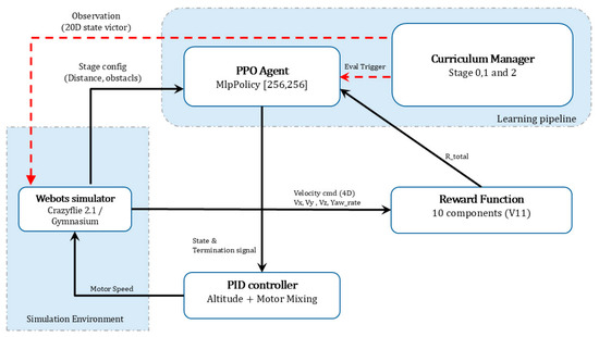
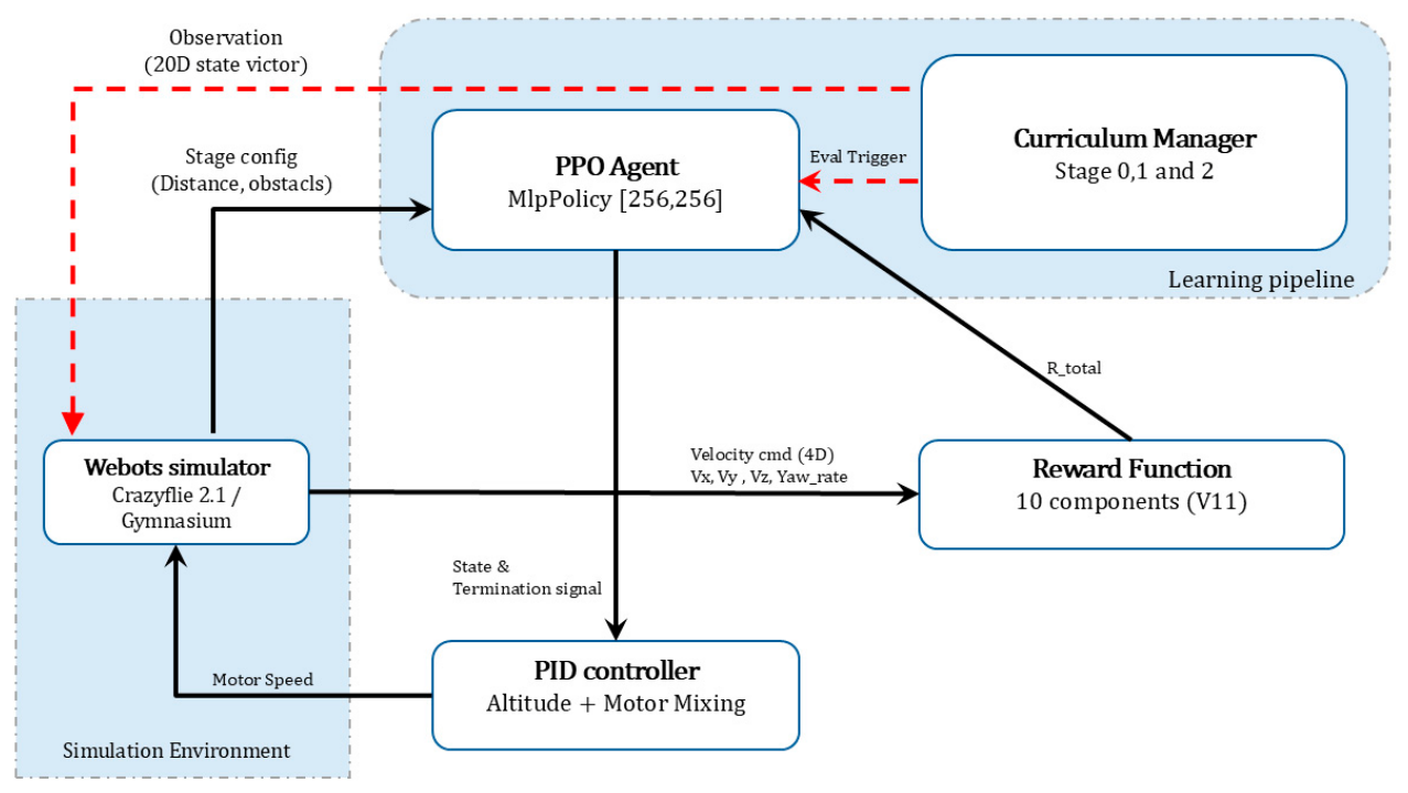
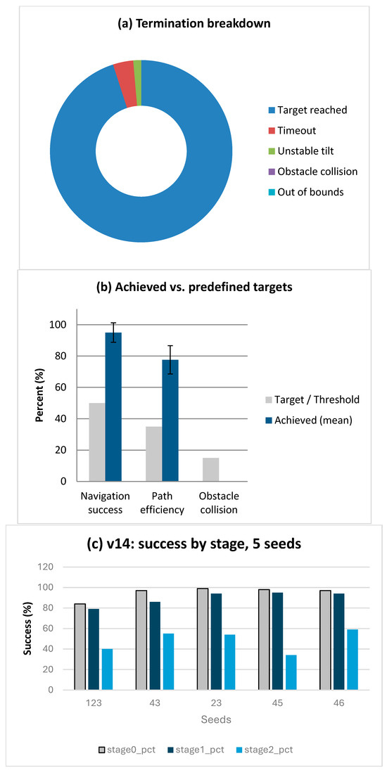
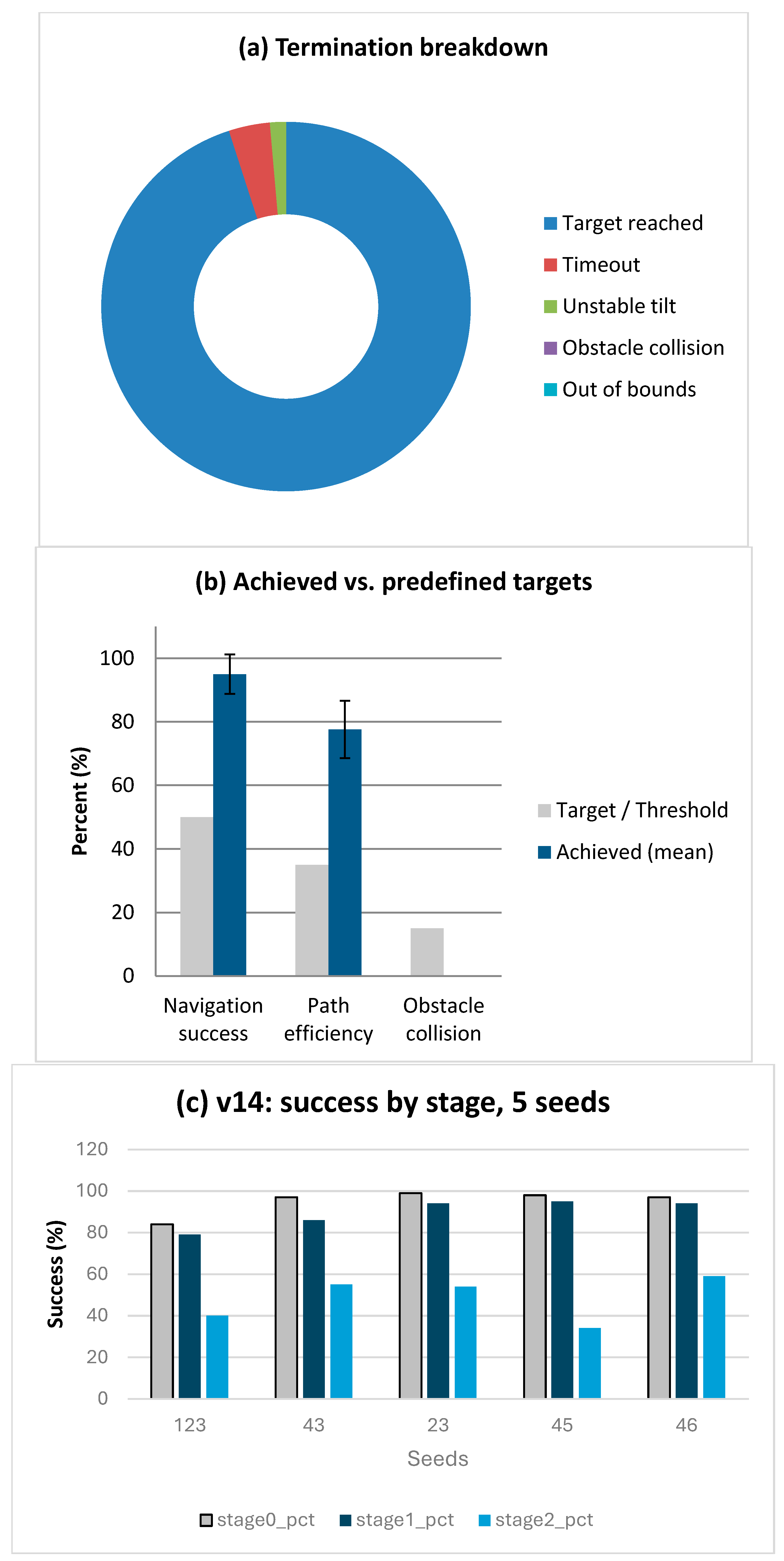
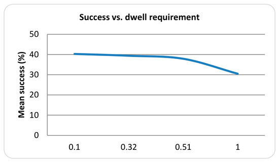
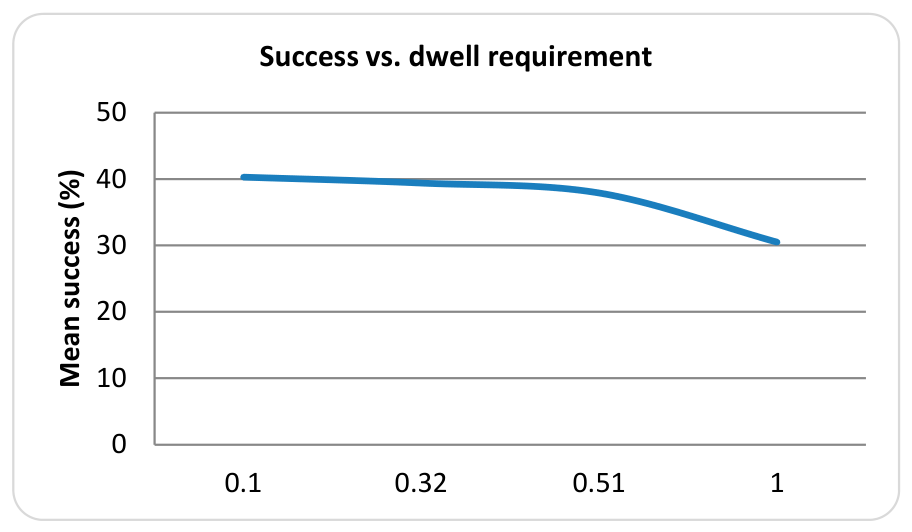
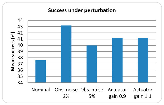
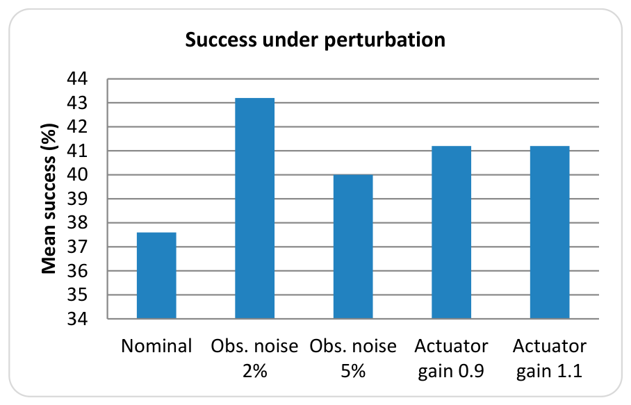

Disclaimer/Publisher’s Note: The statements, opinions and data contained in all publications are solely those of the individual author(s) and contributor(s) and not of MDPI and/or the editor(s). MDPI and/or the editor(s) disclaim responsibility for any injury to people or property resulting from any ideas, methods, instructions or products referred to in the content. |
© 2026 by the authors. Licensee MDPI, Basel, Switzerland. This article is an open access article distributed under the terms and conditions of the Creative Commons Attribution (CC BY) license.