


Highlights
What are the main findings?
- A ResNet18 model based on transfer learning was developed to classify BBCH-defined phenological stages of five crops from low-altitude RGB imagery acquired by UAVs.
- Using 11,489 images of sunflower, rapeseed, soybean, wheat, and barley, the crop-specific models achieved high accuracy on internal test sets, with a mean accuracy of 99.73% under the studied low-altitude UAV imaging conditions.
What are the implications of the main findings?
- The results support the potential of low-altitude UAV imagery and deep learning for localized phenological assessment of selected field zones in precision agriculture.
- BBCH-based labeling with both single stages and stage ranges can represent heterogeneous or transitional field conditions. However, broader deployment requires validation across independent fields, seasons, regions, and survey conditions.
Abstract
This study investigates the automatic classification of crop phenological stages from low-altitude UAV RGB imagery. The dataset included 11,489 images of five crops: sunflower, rapeseed, soybean, wheat, and barley. The images were annotated using the Biologische Bundesanstalt, Bundessortenamt und Chemische Industrie (BBCH) scale, with labels corresponding to either single stages or stage ranges to reflect heterogeneous field conditions and transitional crop states. A pretrained ResNet18 model was adapted to the task using transfer learning. Training was conducted in two stages: first, the classification head was optimized while the backbone remained frozen; second, the entire network was fine-tuned. The model achieved strong internal test accuracy across all crops, with 100% test accuracy for rapeseed and barley, more than 99% for the remaining crops, and a mean accuracy of 99.73% under the studied survey conditions. The results also compare favorably with previously reported studies on UAV-based phenological classification. Overall, the findings support the potential of low-altitude UAV imagery and deep learning for localized phenological assessment of selected field zones in precision agriculture, while broader deployment requires validation across independent fields, seasons, regions, and survey conditions.
1. Introduction
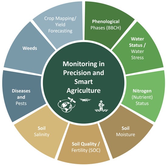
The need to improve the sustainability and productivity of agricultural production in the face of climate change, resource scarcity, and increasing environmental demands is driving the transition from traditional technologies to precision agriculture (PA) [1,2] and smart agriculture (SA) [3]. A key component of these technologies is monitoring, which provides regular spatial and temporal information on the condition of crops, soil, and environmental factors to support decision-making (from work planning to differentiated resource application and outcome forecasting). In the modern literature, the most common monitoring tasks include the following: (1) determining the phenological stages of crop development [4], (2) assessing the water status of plants and water stress to support irrigation decisions [5], (3) monitoring the nutrient (primarily nitrogen) status of crops to optimize fertilizers [6], (4) identifying diseases and pests [7], (5) monitoring weeds for targeted protection [8], (6) crop mapping [9] and forecasting yields based on observation data during the season [10], (7) monitoring soil condition, where along with the water regime, quality/fertility indicators (for example, organic carbon content as an integral indicator) are becoming increasingly important [11], and for arid regions—(8) soil salinization as a factor of degradation and reduced productivity [12,13]. To address these challenges, modern agricultural monitoring utilizes remote, proximal, and ground-based sensing data, which differ primarily in the distance of the sensor from the observed object, spatial coverage, and level of detail. Remote sensing enables regular monitoring of large areas using satellite, aerial, and Unmanned Aerial Vehicle (UAV) platforms, while proximal and ground-based sensing focus on obtaining more detailed measurements near plants and from the field surface, making these approaches complementary in precision and intelligent farming systems [14,15] (Figure 1).
Figure 1.
Key monitoring tasks in precision and smart agriculture using remote and proximal sensing.
This paper addresses the automatic classification of crop phenological stages using low-altitude UAV imagery, a task that is important for optimizing the timing of agronomic interventions and improving yield forecasting [16]. The proposed approach is intended for detailed phenological assessment of selected field zones identified during preliminary large-area monitoring using satellite imagery or higher-altitude UAV.
Traditional methods for determining phenological phases, based on visual observations by experts, are labor-intensive, limiting their use for monitoring large areas. The development of remote sensing technologies, including the use of satellite data and images from unmanned aerial vehicles (UAVs), has significantly expanded the possibilities for collecting information on crop conditions [4,17]. These data provide high spatial and temporal resolution and are widely used in agricultural monitoring.
In recent years, deep learning methods have played a key role in image analysis in agriculture. Reviews [18,19] show that deep learning models demonstrate higher accuracy compared to traditional image processing methods. Convolutional neural networks (CNNs) are widely used for plant image classification and remote crop monitoring [20,21,22]. Pre-trained architectures such as ResNet [23] and detection models of the YOLO family, which have been successfully applied in agricultural tasks [24], can achieve high accuracy even with limited data.
Despite the progress made, automatic classification of phenological stages remains a challenging task in practice. This is due to the high variability in plant appearance, the gradual nature of the transition between stages, and the limited availability of detailed labeled data. Crop heterogeneity further complicates the task: within a single field, plants at different stages of development may be present simultaneously.
In real-world settings, image labeling is often performed at the field level and reflects a mixture of phenological states. Therefore, this study uses an approach in which the label describes the dominant state of the plot and can correspond to either a single stage or a range of stages on the Biologische Bundesanstalt, Bundessortenamt und Chemische Industrie (BBCH) scale. This allows transitional field states to be represented explicitly during annotation.
Accordingly, this study investigates the use of deep learning for automatic classification of the phenological stages of five crops—sunflower, rapeseed, soybean, wheat, and barley—from UAV images labeled according to the BBCH scale, including both single stages and stage ranges. To achieve this goal, the following tasks were completed: dataset formation and labeling, image preprocessing, model development and training based on the ResNet18 architecture, classification quality assessment, and analysis of the obtained results.
The paper is organized into six sections. Section 2, Related Work, provides a focused overview of previous studies relevant to phenological classification of agricultural crops. Section 3 briefly describes the study area, initial data, and methods. Section 4 presents the experimental results, Section 5 discusses the results and limitations, and Section 6 summarizes the work and outlines directions for further research.
2. Related Work
Previous studies have addressed crop phenological classification using manual field observations, semi-automated proximal sensing, satellite time series, and image-based approaches, including UAV and ground-based imagery [14,16,25,26,27]. These studies demonstrate that phenological information can be derived from different sensing platforms and modeling strategies, but performance and transferability depend strongly on data type, spatial and temporal resolution, labeling strategy, and validation design.
2.1. Methods of Phenological Classification
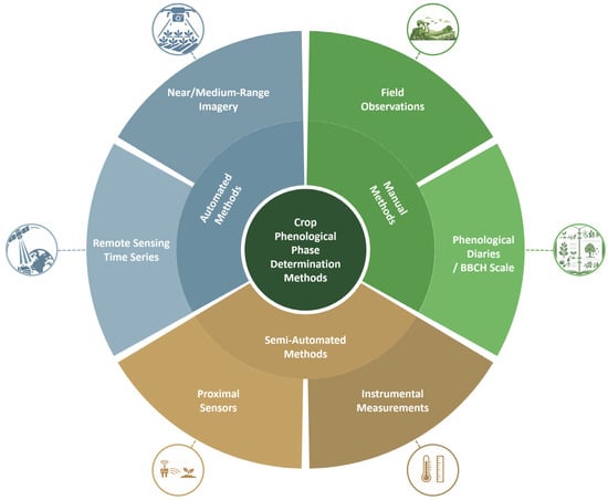
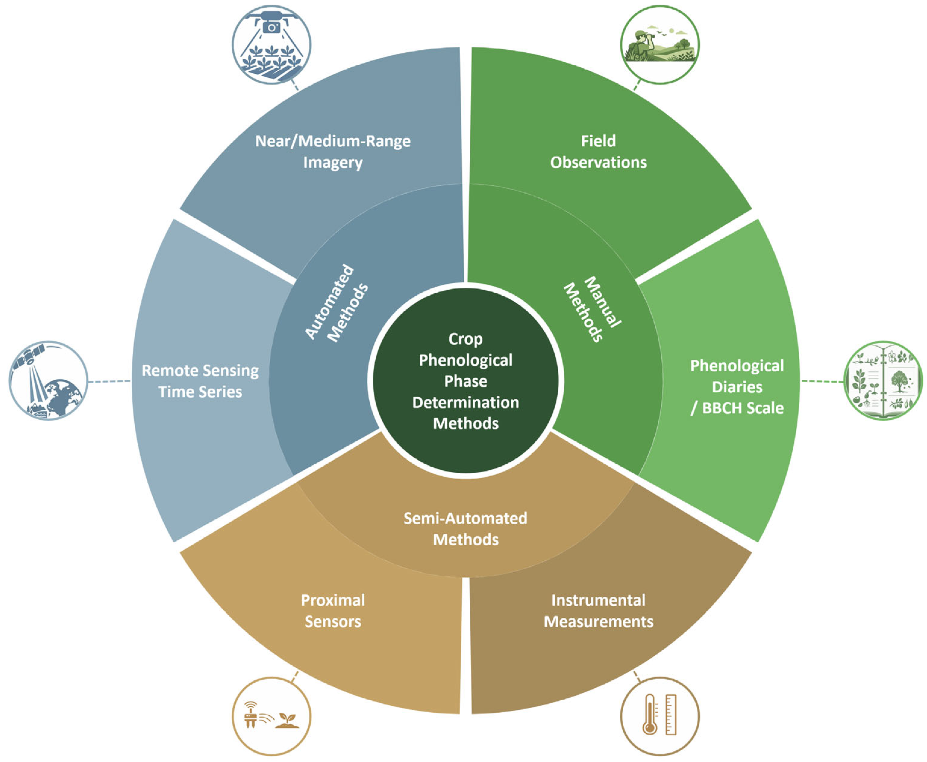
For clarity, phenological classification methods can be grouped by the degree of automation and the type of data used (Figure 2). Manual methods include visual observations by experts in the field, the use of phenological diaries and scales, particularly the BBCH scale, as well as protocols for selective crop sampling [25].
Figure 2.
Classification of methods for determining crop phenological stages: manual, semi-automated, and automated approaches.
Manual observations are biologically interpretable and can capture transitional states, but they are labor-intensive, subjective, and difficult to scale. Semi-automated methods combine visual observations with proximal or handheld measurements and determine the stage using selected features or rules [14].
Automatic approaches can be divided into methods based on remote sensing time series and methods based on near- or mid-range imagery. Time-series methods use spectral-index dynamics, threshold rules, seasonal-curve approximations, and machine learning models such as Support Vector Machines (SVMs) and k-Nearest Neighbors (kNNs) [4,28], as well as deep learning and transformer-based architectures [29,30].
Phenological normalization of the time axis can improve model portability [31]. However, satellite-based approaches remain limited by spatial resolution, cloudiness, and mixed pixels, especially in heterogeneous fields and small plots.
Image-based approaches determine phenology from plant morphology and canopy structure using ground cameras, PhenoCam systems, mobile imagery, or UAV data. PhenoCam studies combine CNN classification with temporal post-processing such as Hidden Markov Models to obtain robust daily field-state sequences [32,33]. UAV imagery provides lower temporal continuity but much higher spatial resolution, enabling plant- or row-level analysis and detection of within-field heterogeneity [16,34]. Image-based phenological tasks include scene classification [35], organ detection [24], and segmentation-based analysis [20].
2.2. Machine Learning Methods for Phenological Classification
Early automated phenological classification relied on manually designed spectral, textural, and canopy features followed by classical machine learning methods, including SVM and kNN [28]. Such methods can perform well under stable conditions, for example, in sugarcane stage identification from Sentinel-2 vegetation-index time series [36], but their transferability between regions and seasons is limited by differences in cultivars, management, weather, and phenological timing.
Recent studies increasingly use deep learning, attention mechanisms, and temporal models. For UAV orthomosaics, MaizeHT combines CNNs and self-attention and reaches 97.7–98.7% accuracy in maize growth-stage recognition [35]. ResNet-50 has been applied to rice growth-stage classification from ground images [37], while CNN-LSTM and CNN-GRU models are used when image sequences are available [38]. For PhenoCam imagery, DL classification combined with HMM post-processing improves temporal consistency under management events such as plowing, harvesting, and crop rotation [32].
2.3. Phenological Classification Using UAV Data and Deep Learning
For the present study, the most relevant works are those that classify phenological stages directly from UAV RGB or multispectral imagery using deep learning. Reviews confirm that UAVs are valuable for such tasks because they combine high spatial resolution, flexible survey timing, and operation below cloud cover [17,18]. However, adjacent phenological stages often differ only in subtle morphological details, so classification errors commonly occur between neighboring classes [39,40].
A further limitation concerns data and labeling. Many studies rely on local datasets collected in one region with a fixed sensor and survey protocol, which may overestimate performance because of hidden correlations in background, illumination, and management conditions. Consequently, practical deployment requires attention to domain shifts and stronger evaluation protocols such as leave-one-field or leave-one-season-out validation [41].
In Central Asia, including Kazakhstan, UAV-based phenological classification remains underrepresented despite the region’s agro-climatic diversity and the importance of grain and oilseed production. A relevant dataset for wheat, barley, and soybean in East Kazakhstan has been published using multispectral UAV imagery [42]. Related studies from Kazakhstan also show the potential of UAVs and machine learning methods for soybean plant and weed detection [24] and agricultural salinity mapping [13], but available datasets remain limited in crops, years, and survey conditions. Standardized BBCH labeling is therefore important for comparability and for representing mixed field states [25].
Overall, recent research highlights several persistent limitations:
- Weak separability of adjacent stages and continuous transitions between phases [36,38,40];
- Heterogeneous crop states within a field, which complicate the assumption of one stage per image [28];
- Limited availability of labeled BBCH datasets covering different seasons, cultivars, regions, and management conditions [42];
- Limited transferability between regions, crops, and sensors, requiring phenological normalization, robust evaluation protocols, or transfer learning [31,41,43].
A broader comparison of related machine-learning-based classification and prediction tasks is provided in Appendix A, including growth-stage recognition, BBCH estimation, and maturity prediction.
The proposed approach responds to these limitations by using UAV data collected in Kazakhstan, applying BBCH-based labels that retain stage ranges across heterogeneous field states, and employing transfer learning with a ResNet architecture [23]. The study also considers several crop groups within one experimental framework, providing a basis for future studies aimed at developing more transferable multi-crop phenological models [18,19,42].
3. Materials and Methods
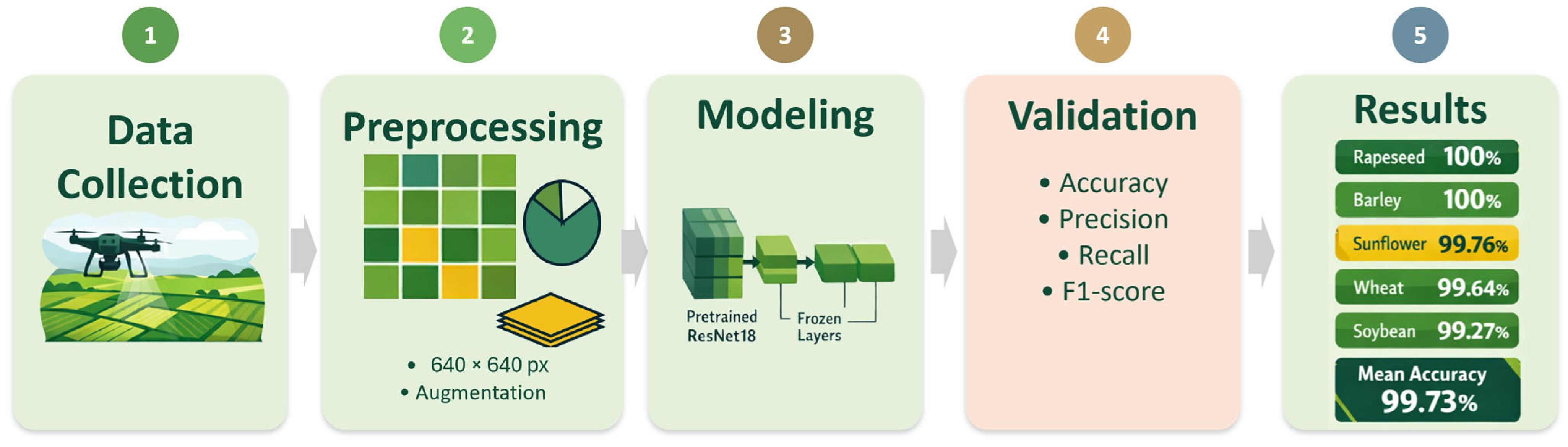
The study followed the workflow shown in Figure 3. Initially, a set of UAV images of agricultural crops was collected and compiled, after which the data was labeled using the BBCH scale, taking into account both individual stages and their ranges.
Figure 3.
Research workflow.
Next, we preprocessed and augmented the images, prepared the training, validation, and test sets, and then trained the models based on the ResNet18 architecture using a transfer learning strategy. The final step was to assess the classification quality using standard multi-class classification metrics. The individual stages of the research workflow shown in Figure 3 are described step by step in Section 3.1, Section 3.2, Section 3.3, Section 3.4 and Section 3.5, including initial data preparation, preprocessing and augmentation, model architecture, training, and evaluation metrics.
3.1. Initial Data
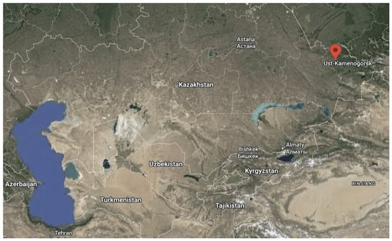
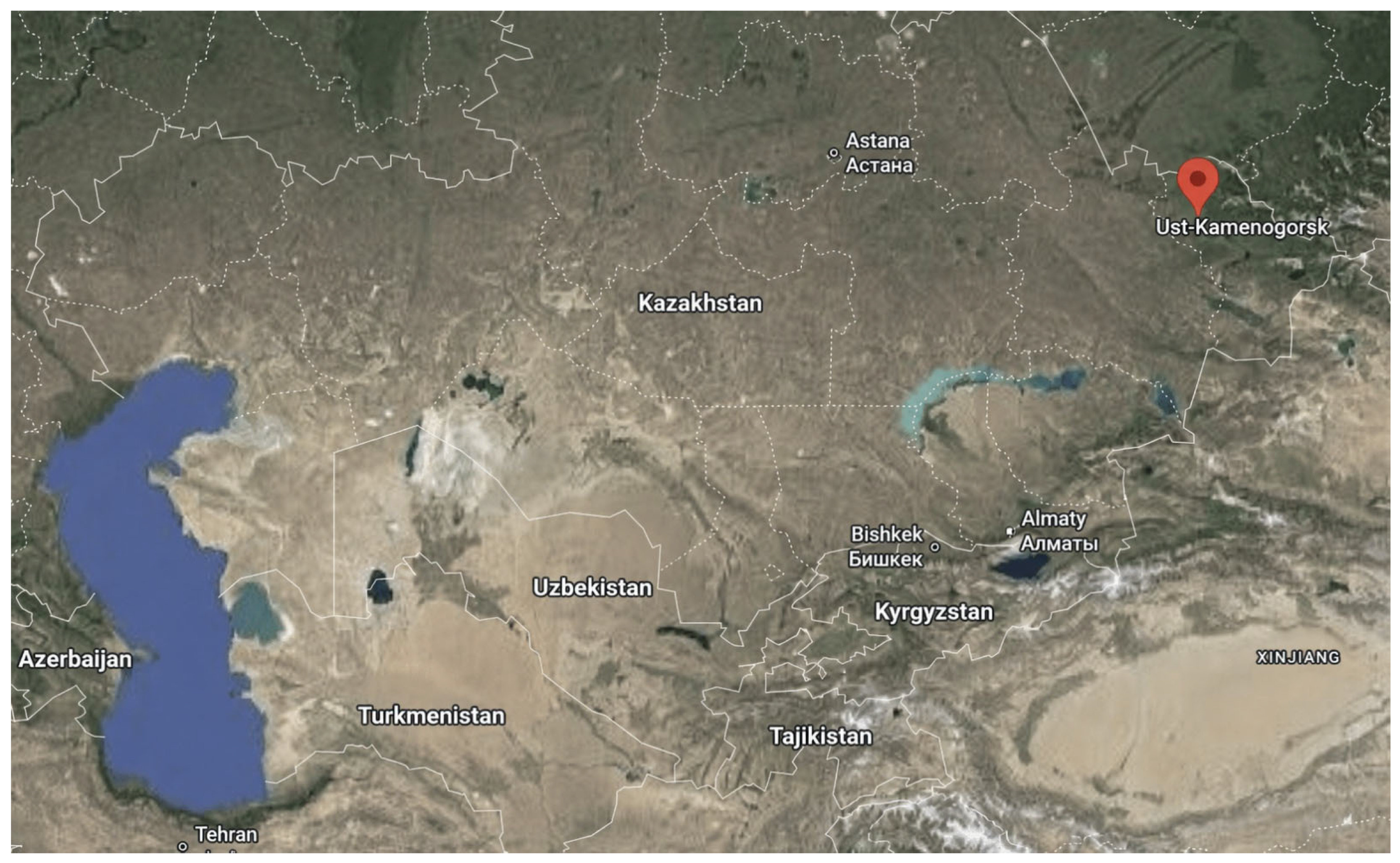
A dataset of UAV images was compiled for five crops: sunflower, rapeseed, soybean, wheat, and barley. The total number of images was 11,489. The surveys were conducted in agricultural fields near Ust-Kamenogorsk (Kazakhstan), in the village of Vinnoye, and on land owned by Aitas Agro LLC. The geographic coordinates of the survey area are approximately 50°03′ N, 82°50′ E (Figure 4).
Figure 4.
Location of the plant image acquisition site in East Kazakhstan.
The fields where the aforementioned crops are cultivated are located in the rainfed agriculture zone of Eastern Kazakhstan and are primarily occupied by spring wheat and barley, as well as oilseeds (sunflower, rapeseed) and soybeans. The soil cover is predominantly alkaline and ordinary chernozems (in some places, dark chestnut). The climate of the region is sharply continental (humid continental according to Köppen–Geiger, Dfb): the average annual temperature is approximately 4.2 °C, the annual precipitation is approximately 600 mm, the average January temperature is ≈−14.7 °C, and the average July temperature is ≈20.7 °C [44].
The images of the fields were obtained using a DJI Mavic 3E drone (SZ DJI Technology Co., Ltd., Shenzhen, China) equipped with a 20 MP wide-angle 4/3 CMOS camera with a 24 mm equivalent focal length, an adjustable aperture of f/2.8–f/11, and a mechanical shutter [45].
Flights were conducted at altitudes of 3–10 m to capture detailed images of individual plants. The camera was oriented primarily vertically downwards (tilt angle of approximately –80° to –90°), corresponding to nearly orthogonal imaging.
The dataset consisted of original UAV photographs acquired during field flights, mainly without overlap or with only limited overlap of approximately 10–20% between neighboring images; no additional overlapping cropped fragments were generated from the same photographs.
The UAV image campaigns were conducted during the 2025 growing season, from 18 June to 11 August. The acquisition period covered June, July, and August and comprised 15 distinct calendar dates and 32 UAV acquisition sessions. The crop-level and BBCH-stage-level distribution of fields, survey dates, UAV sessions, image counts, and acquisition times are provided in Appendix B.
Synchronized field-level meteorological measurements were not collected during the UAV surveys. Therefore, temperature, wind speed, cloud cover, and precipitation were not included as experimental covariates, which limits the assessment of model robustness to weather-related variability in illumination and canopy appearance.
The BBCH scale [25] was used as the unified coding system for plant development stages, enabling consistent annotation and comparison of phenological stages across the studied crops.
Data labeling was performed at the field-survey level: all images obtained during a single survey were assigned a single label corresponding to the dominant phenological stage or range of plant development stages in the field as a whole. Therefore, classes could represent both individual stages (e.g., “19”) and phase intervals (e.g., “16–19,” “19–30”), reflecting the heterogeneity of crops. The BBCH annotations were prepared by two agronomists. When the crop state was visibly heterogeneous or transitional, a BBCH interval was used instead of forcing the survey dataset into a single-stage class. Thus, BBCH intervals represent intentionally retained stage ranges within a field survey. A formal numerical inter-annotator agreement coefficient was not calculated during dataset preparation.
The overall composition of the dataset and the distribution of images by phenological stages are presented in Table 1. The number of BBCH stages varies for different crops: 9 stages are allocated for sunflower, 5 for soybeans, 3 for rapeseed, 6 for wheat, and 4 for barley.
Table 1.
Datasets used for training phenological stage classification models.
Although wheat and barley are morphologically similar cereal crops, their class definitions were not forced to be identical because the available field surveys covered different observed BBCH stages and stage ranges for the two crops. The class set for each crop was therefore determined by the actual phenological states represented in the collected images rather than by a predefined common cereal-stage scheme. This crop-specific labeling strategy avoided introducing artificial or poorly represented classes and ensured that each model was trained only on stages that were sufficiently represented in the corresponding dataset.
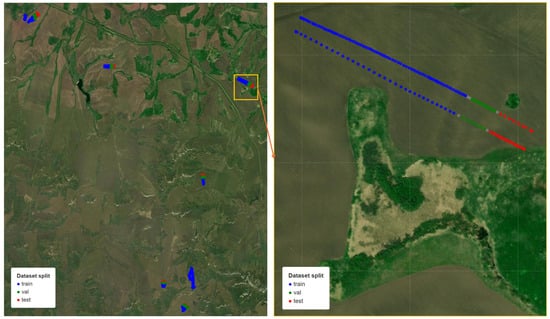
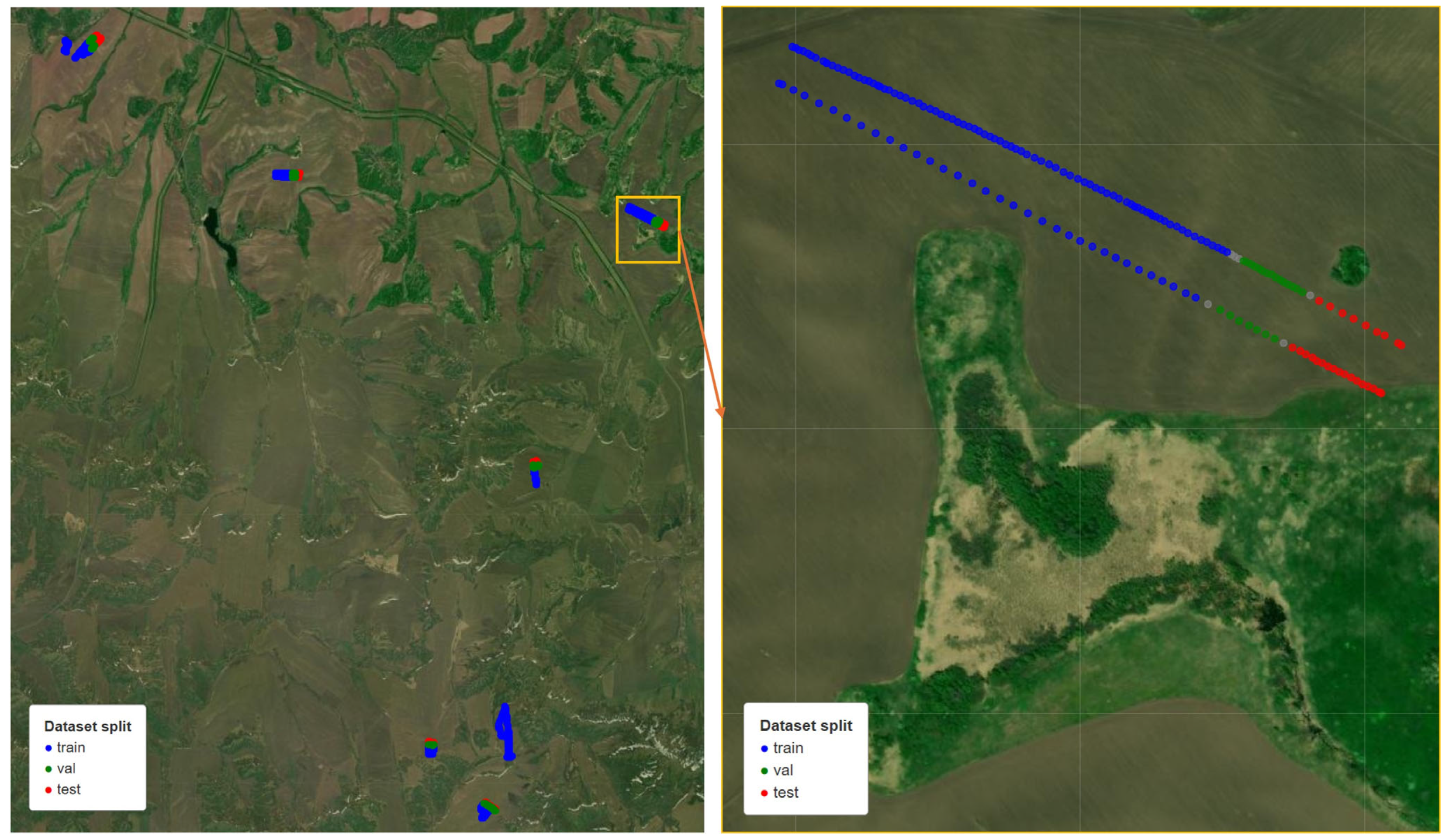
The data were divided into training, validation, and test sets (70:15:15) using GroupShuffleSplit. Each data source/field-survey group was assigned to only one subset, preventing images from the same local survey group from being shared between the training, validation, and test sets. This group-based split reduced the risk of data leakage caused by visually similar images acquired from the same field area or survey sequence. The spatial distribution of the split is illustrated for sunflower in Figure 5, and the corresponding split maps for all crops are provided in the Supplementary File dataset_splits_map.html. The training set was used to optimize model parameters, the validation set was used to select hyperparameters and monitor the training process, and the test set was used exclusively for the final evaluation of classification performance. A separate model was trained for each crop, allowing crop-specific hyperparameter tuning and avoiding class imbalance across crops.
Figure 5.
Spatial distribution of sunflower UAV images assigned to the training, validation, and test subsets. The figure illustrates the group-based split used to reduce data leakage risk by avoiding the allocation of images from the same local survey group to different subsets.
3.2. Data Preprocessing and Augmentation
Before feeding the images into the neural network, they underwent a preprocessing step. All images were scaled to a size of 224 × 224 pixels, corresponding to the input size of the ResNet architecture.
To improve the generalization ability of the model, data augmentation methods were used. Augmentation was performed exclusively on the training set, while the validation and test sets were used without any additional transformations, ensuring an accurate assessment of the model’s quality.
The following transformations were used as part of the augmentation:
- Random horizontal reflection (probability 0.5);
- Random rotation in the range of ±15°.
After augmentation, the images were normalized using the mean and standard deviations of the RGB color channels calculated for the ImageNet dataset:
- Mean = [0.485, 0.456, 0.406];
- Std = [0.229, 0.224, 0.225].
This normalization ensures that the distribution of the input data matches the distribution on which the model was pretrained, which promotes more efficient training.
3.3. Model Architecture
The ResNet18 [23] architecture, a convolutional neural network pretrained on the ImageNet dataset, was used as the classification model. The ResNet architecture is based on the use of residual connections, which allow for the efficient training of deep neural networks.
ResNet18 was selected because it offers a practical balance between model capacity, training stability, and computational efficiency. Its residual connections support stable fine-tuning, while ImageNet pretraining provides reusable visual features relevant to crop color, texture, and canopy structure. During preliminary development, ResNet18 was compared with a lightweight custom SimpleCNN baseline and showed more stable and reliable performance. This comparison was used for model selection and was not intended as an exhaustive benchmark against other CNN or transformer architectures.
The ResNet18 model consists of an initial convolutional layer followed by four sequential residual blocks. Each block contains two convolutional layers with a ReLU activation function and batch normalization layers. Finally, the network is terminated with global average pooling and a fully connected classification layer.
To solve the problem of classifying crop phenological stages, the basic architecture was modified (Figure 6). The final fully connected layer was replaced with a layer with a number of output neurons corresponding to the number of classes for a specific crop. Thus, the number of output classes was as follows:
- Sunflower—9;
- Rapeseed—3;
- Soybean—5;
- Wheat—6;
- Barley—4.
Figure 6.
ResNet18-based architecture for UAV crop phenology classification.
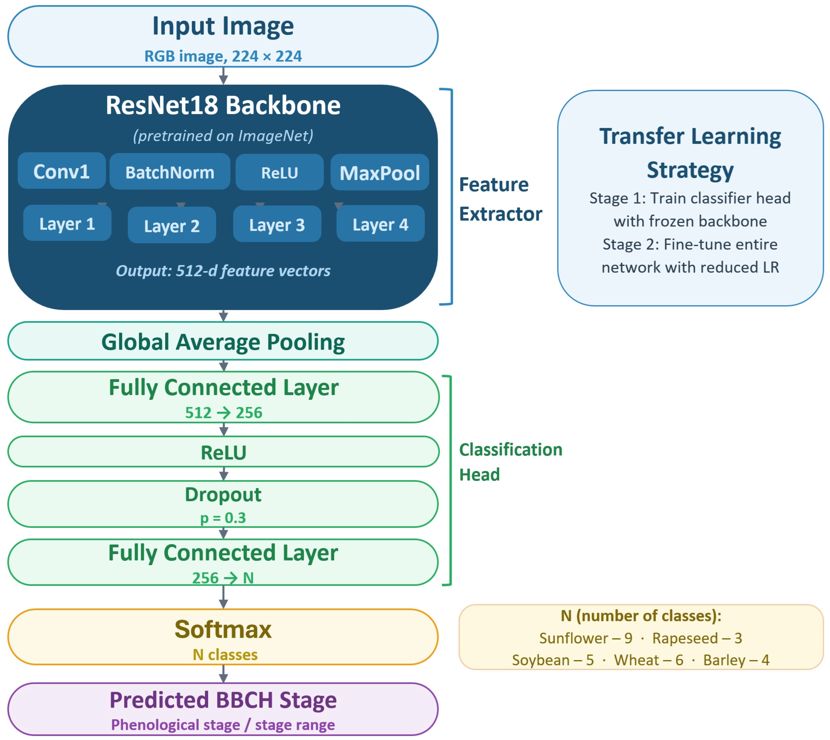
To reduce overfitting in the classification part of the model, a Dropout layer with a probability of 0.3 was used.
3.4. Model Training
Models were trained using the AdamW optimizer (weight decay = 1 × 10⁻⁴). The main hyperparameters are as follows:
- Learning rate—0.001;
- Batch size—32;
- Number of epochs—10;
- Loss function—Cross-Entropy Loss.
Training was conducted in two stages using a transfer learning strategy. In the first stage (feature extraction), only the output classification layer was trained with frozen base network weights. All layers of the ResNet18 architecture, except for the last fully connected layer, were fixed (including conv1, bn1, and blocks layer1–layer4). Only the upper part of the network remained trainable, represented by a sequence of layers: Linear (512→256) → ReLU → Dropout (regularization layer) → Linear (256→N), where N is the number of classes. The total number of trainable parameters at this stage was approximately 131,000 out of ~11.3 million. Training at this stage was conducted over 7 epochs.
In the second stage (fine-tuning), the network was completely unfrozen, followed by retraining of all model parameters. To prevent degradation of the pre-trained weights, the learning rate was reduced by a factor of 10 relative to the initial value. Retraining was performed over three epochs.
To ensure reproducibility of the results, the random number generator seed (random seed = 42) was fixed in all experiments for the NumPy (2.5.0), PyTorch (2.12.1+cu130), and the standard random modules.
The selection of training parameters was based on preserved preliminary experiments. For ResNet18, the main grid evaluated learning rates of 10−4, 5 × 10⁻⁴, and 10−3 with batch sizes of 16, 32, and 64. The final settings were selected from these experiments, which are summarized in Appendix B, Table A3.
Model training and inference were performed using CUDA (13.2) acceleration on an NVIDIA (Santa Clara, CA, USA) GeForce RTX 3070 Ti Laptop GPU with 8 GB of VRAM. Mixed-precision training, implemented using torch.cuda.amp (2.12.1+cu130), was used to accelerate computations. Training time for each model was approximately 7–10 min.
3.5. Evaluation Metrics
Standard multi-class classification metrics were used to assess classification quality:
- Accuracy—the proportion of correctly classified images;
- Precision—the proportion of correct predictions within each class;
- Recall—the proportion of correctly identified positive examples;
- F1-score—the harmonic mean of Precision and Recall.
The metrics were calculated on the test set for each crop separately.
4. Classification Results
The classification results for each crop studied are presented below.
4.1. Sunflower
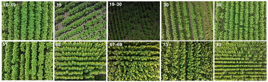
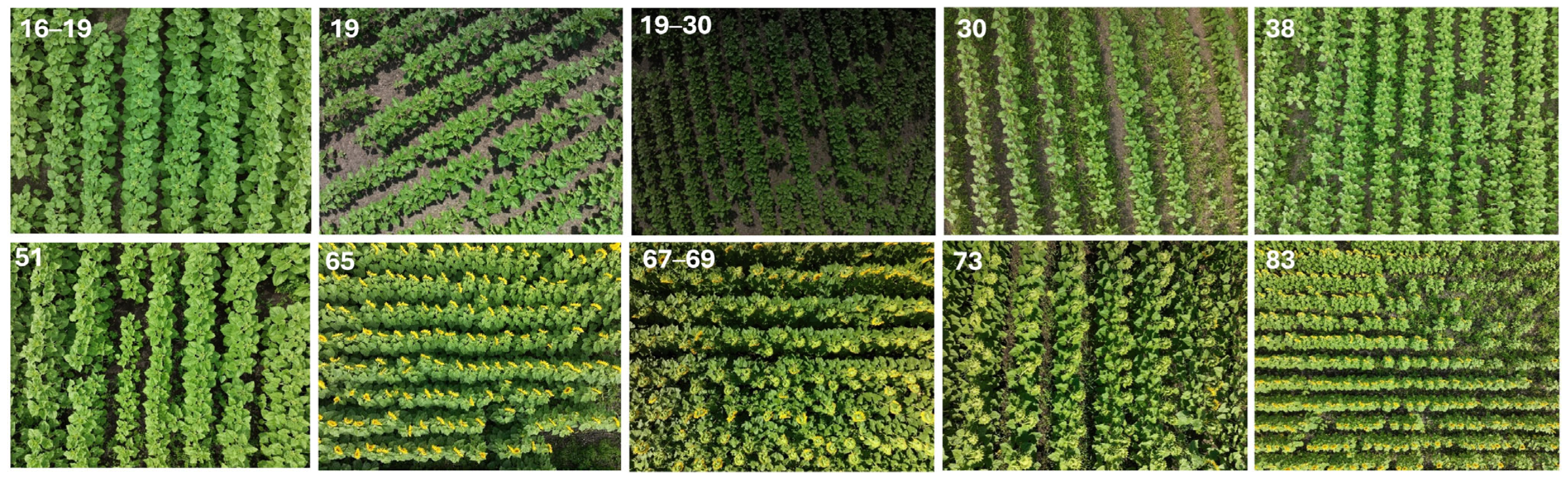
Sunflower had the largest number of classes (nine), making it the most challenging classification task among the studied crops. Despite this, the model demonstrated high accuracy for most phenological states. Representative sunflower images corresponding to the analyzed BBCH stages will be presented in Figure 7.
Figure 7.
Representative UAV RGB images of sunflowers at the analyzed BBCH phenological stages.
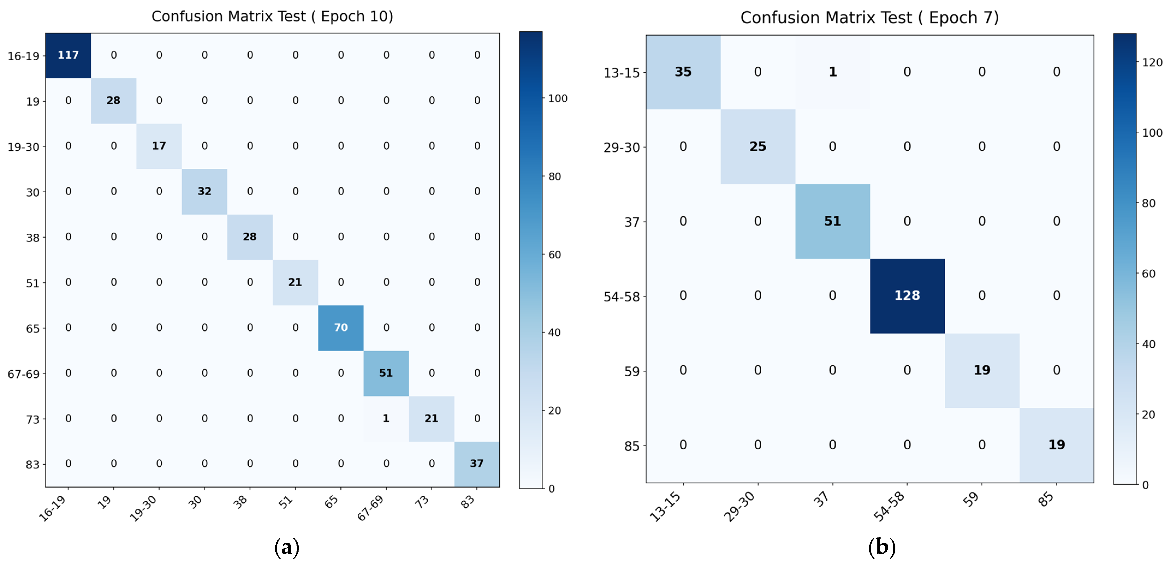
A slight decrease in quality is observed for stages 67–69 and 73 (F1-score 0.99 and 0.98, respectively), which correspond to the late stages of flowering and seed formation. This is explained by the weak visual differences between adjacent stages.
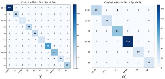
Analysis of the confusion matrix (Figure 8a) reveals a single error: one sample at stage 73 was classified as a 67–69 sample.
Figure 8.
(a) Sunflower confusion matrix; (b) wheat confusion matrix.
Given the proximity of these stages, this error is expected. Detailed metric values are presented in Table 2.
Table 2.
Sunflower stage classification metrics.
4.2. Wheat
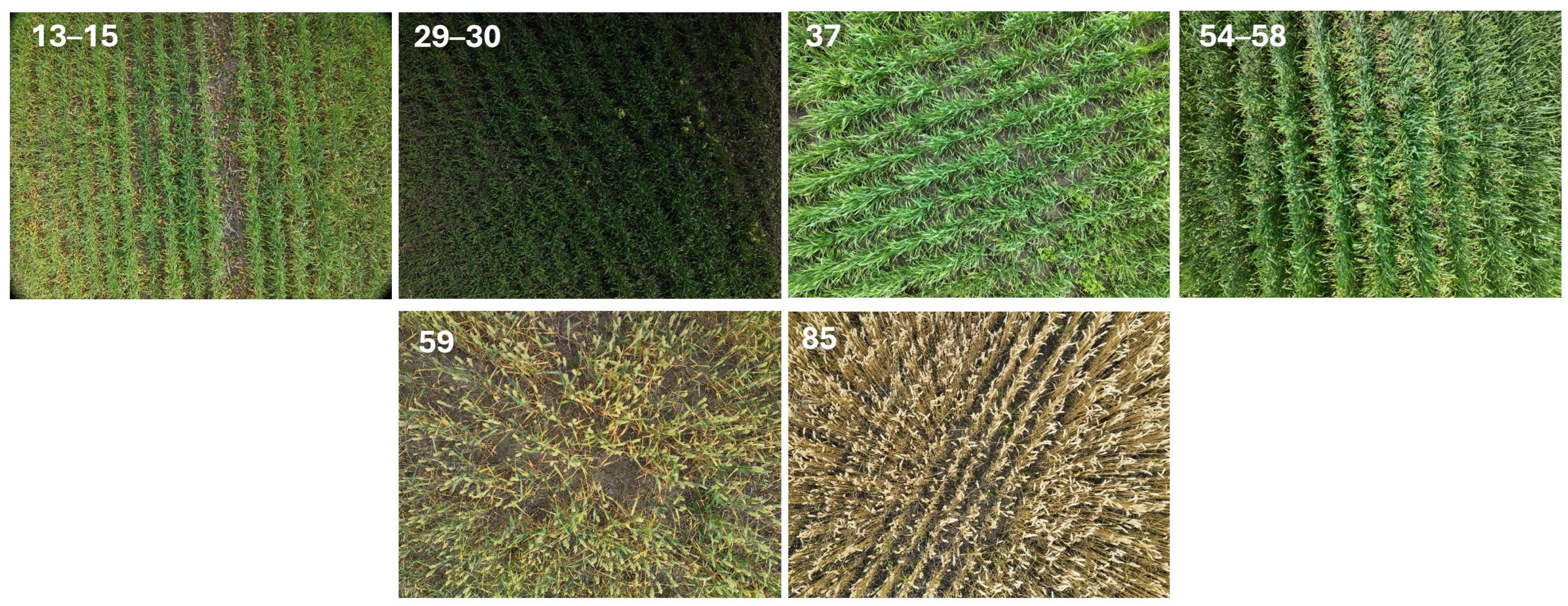
Six phenological stages are considered for wheat. The model demonstrates high accuracy for all classes (Table 3), with a slight decrease in F1-score (0.98) observed for stage 85, which is late in ripening.
Table 3.
Wheat stage classification metrics.
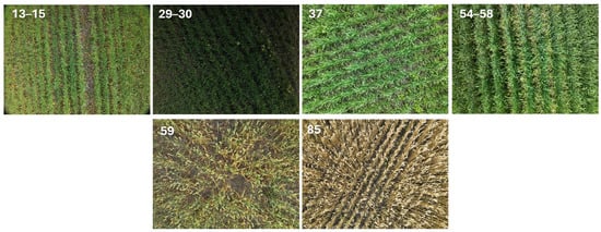
Representative wheat images corresponding to the analyzed BBCH stages will be presented in Figure 9.
Figure 9.
Representative UAV RGB images of wheat at the analyzed BBCH phenological stages.
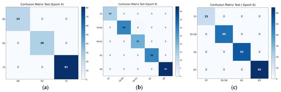
According to the confusion matrix (Figure 8b), one error was detected: a sample from stages 13–15 was classified as stage 37.
4.3. Rapeseed
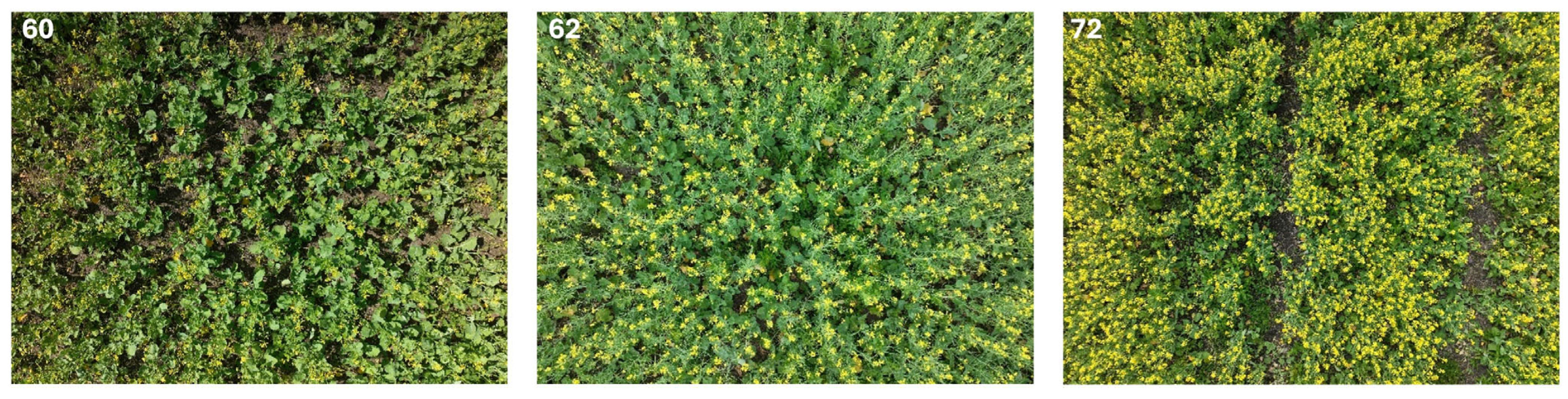
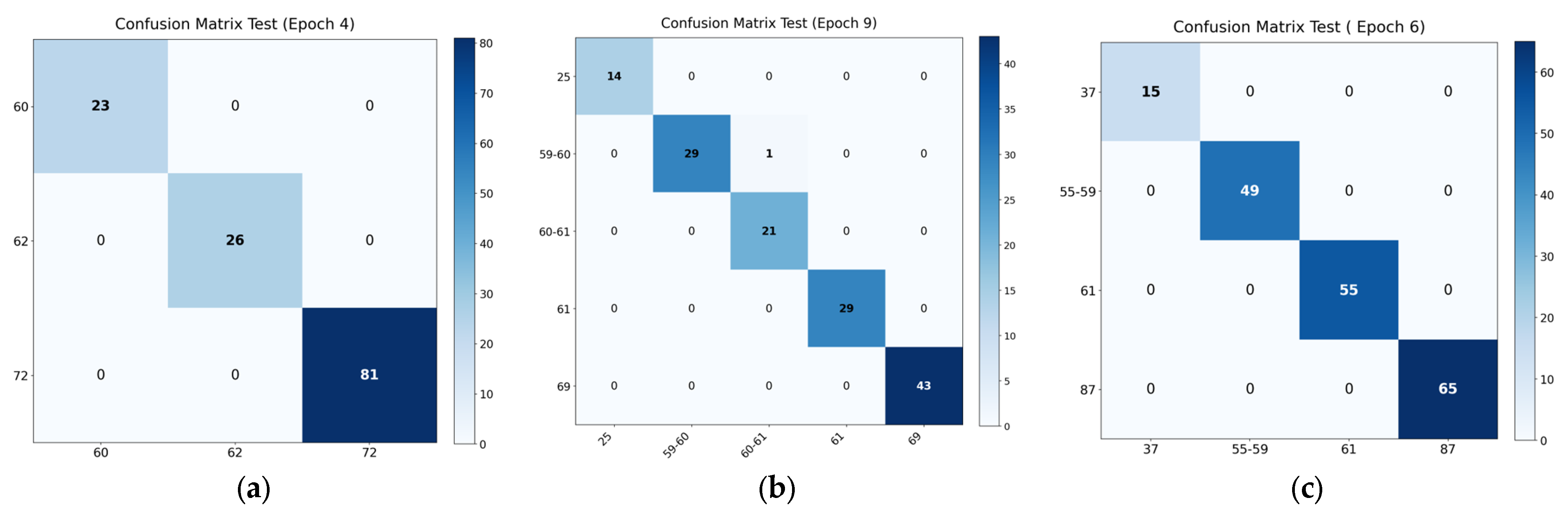
Three phenological stages were analyzed for rapeseed: 60, 62, and 72. The classification results are presented in Table 4.
Table 4.
Rapeseed stage classification metrics.
For all stages considered, the model achieved maximum values for the Precision, Recall, and F1-score metrics.
Representative rapeseed images corresponding to the analyzed BBCH stages are shown in Figure 10.
Figure 10.
Phenological stages of rapeseed development. Stage numbers are shown in the upper left corner of each image.
The confusion matrix (Figure 11a) shows a complete absence of classification errors in the test set. This is likely due to the small number of classes and the clearly distinguishable morphological features of the corresponding stages.
Figure 11.
(a) Rapeseed confusion matrix; (b) soybean confusion matrix; (c) barley confusion matrix.
4.4. Soybean
Five phenological stages are analyzed for soybean. The model provides high accuracy, with a slight decrease in F1-score (to 0.99) observed for stages 60–61. Representative soybean images corresponding to the analyzed BBCH stages will be presented in Figure 12.
Figure 12.
Representative UAV RGB images of soybean at the analyzed BBCH phenological stages.
The confusion matrix (Figure 11b) shows a single error: a sample at stage 59–60 was classified as 60–61. The two stages are adjacent, and their visual differences are weak, which explains this discrepancy.
Detailed results are presented in Table 5.
Table 5.
Soybean stage classification metrics.
4.5. Barley
Four phenological stages were analyzed for barley. Maximum metric values were obtained for all classes (Table 6), and there were no classification errors (Figure 11c). Representative barley images corresponding to the analyzed BBCH stages will be presented in Figure 13.
Table 6.
Barley stage classification metrics.
Figure 13.
Representative UAV RGB images of barley at the analyzed BBCH phenological stages.
5. Discussion
Table 7 presents the summary results of phenological stage classification for all studied crops. The ResNet18 model demonstrated high accuracy in classifying phenological stages for all studied crops. The highest scores were obtained for rapeseed and barley, for which classification accuracy on the test set was 100%. Accuracy for sunflower, wheat, and soybean was also high, exceeding 99%. The average accuracy across all crops was 99.73%. These values should be interpreted in the context of the experimental design: rapeseed and barley had relatively few classes, the corresponding stages were visually well separated, and the images were acquired under comparatively homogeneous low-altitude UAV survey conditions.
Table 7.
Summary classification results by crop.
Another factor that may have contributed to the high accuracy is the use of separate crop-specific models. This design reduced the complexity of the classification task compared with a single universal multi-crop model and allowed the output layer and training procedure to be adapted to the number of BBCH classes available for each crop.
These results indicate that the proposed approach can distinguish the studied crop-stage combinations. At the same time, the values in Table 7 should be interpreted together with the crop-specific class structure, visual separability of the analyzed stages, and relatively homogeneous acquisition conditions.
To further examine the generalizability of the sunflower model, an additional external evaluation was performed using newly acquired sunflower UAV photographs from field locations, dates, and survey sessions that were absent from the original model-development dataset (Table 8). The trained sunflower model was kept frozen, and no additional fine-tuning was performed. Because the additional dataset was limited in size and included only two BBCH intervals, the results should be treated as preliminary external validation rather than as a full leave-one-field/date/session-out benchmark.
Table 8.
Performance of the frozen sunflower model on newly acquired external survey data.
The frozen sunflower model achieved an overall weighted accuracy of 90.48% and a weighted F1-score of 0.9471 on the external set. This lower accuracy compared with the original internal sunflower test accuracy supports a more cautious interpretation of the near-perfect internal metrics and indicates the need for further validation on independent fields, dates, seasons, and locations.
A comparison with studies using satellite data and classical machine learning methods suggests that the higher spatial resolution of UAV imagery may provide an advantage for phenological-stage discrimination in the studied setting. For example, for maize, when recognizing phenological stages from Sentinel images, the best classical models (LD, SVM, kNN) provided an accuracy of approximately 82.3% [28], while for sugarcane, when using Sentinel-2 vegetation-index time series and kNN, Random Forest, SVM, and Naïve Bayes algorithms, the maximum accuracy was 92.45% [36]. These differences should be interpreted with caution because the compared studies differ in crops, sensors, spatial resolution, classification schemes, and validation protocols.
Comparison with recent deep learning studies shows that the performance values obtained in the present study are comparable to or higher than those reported in previously published studies. In rice phenological-stage recognition from RGB images acquired by a terrestrial camera, the ResNet-50 architecture provided an accuracy of about 87.33% [37]. For maize UAV orthophotos, the hybrid CNN + Self-Attention MaizeHT model achieved 97.71–98.71% accuracy [35], and an improved YOLOv6-based model for maize phenological-stage identification from UAV images reported mAP75 = 80.5% and recall = 98.57% [40]. In grape growth-stage recognition, the best ResNet-based architecture provided an average accuracy of 88.1% [39]. However, these comparisons should be interpreted in light of differences in datasets, crops, sensors, and evaluation metrics.
However, direct quantitative comparison between studies is limited by differences in problem formulation, data types, and evaluation metrics. For example, in a study on wheat phenology monitoring using UAV time series, spatiotemporal CNN-GRU and CNN-LSTM architectures were evaluated through BBCH estimation using the coefficient of determination and RMSE rather than multiclass classification accuracy [38]. Similarly, a soybean study addressed maturity-date prediction using multispectral UAV imagery; the best transfer learning strategy yielded R2 = 0.74–0.79 and an RMSE of 1.70–1.96 days [43]. These differences prevent the comparison from being interpreted as a strict ranking of methods. Nevertheless, the combination of UAV data, deep learning, and transfer learning indicates potential for phenological monitoring, while further validation is required for broader deployment.
The use of RGB imagery in this study was intentional because UAVs equipped with RGB cameras are relatively inexpensive, widely available, and easier to deploy in practical agricultural monitoring than systems equipped with multispectral or hyperspectral sensors. However, RGB images mainly capture visible crop appearance and do not directly provide physiological information such as chlorophyll content, canopy biochemical properties, or plant water status. Multispectral and hyperspectral imagery could therefore further improve phenological-stage classification by adding spectral features, including near-infrared, red-edge, and narrow-band reflectance information related to vegetation condition and stress responses. Accordingly, multisensor data fusion is considered a promising direction for future work. In practical applications, such detailed low-altitude surveys may be focused on representative or problematic field zones identified during an initial large-area monitoring stage.
From an operational perspective, the present acquisition protocol should therefore be interpreted as a low-altitude plot- or local-area phenological assessment rather than as whole-field operational mapping. At an altitude of 3–10 m, the DJI Mavic 3E RGB camera used in this study, with a 24 mm-equivalent lens, 4:3 image aspect ratio, and 5280 × 3956 pixel images, provides an approximate nadir footprint of 4.5 × 3.4 m to 15.0 × 11.3 m and an approximate ground sampling distance of 0.85–2.84 mm pixel−1. These values are theoretical and may vary with canopy height, terrain, camera tilt, and altitude-reference accuracy. Such imaging provides detailed top-canopy morphology but requires substantially more images to cover an entire commercial field than a conventional higher-altitude mapping flight. Moreover, nadir RGB images incompletely represent vertical traits such as plant height, ear position, and pod development. Operational whole-field validation should therefore quantify coverage rate, battery use, flight duration, storage requirements, and the benefit of additional oblique or multisensor observations.
The experiments were conducted under relatively favorable weather and imaging conditions. Consequently, factors such as illumination variability, cloud cover, camera viewing angle, shadows, haze, and soil background were not investigated explicitly in the present study. Previous studies have shown that variable illumination, shadow effects, and image degradation may influence UAV-based image analysis, while image enhancement and illumination-correction procedures can improve robustness under changing acquisition conditions [46,47,48,49]. Therefore, evaluating the influence of these factors and corresponding normalization strategies remains an important direction for future research.
The above-mentioned experimental factors, together with the limited geographic scope of the dataset, restrict the extent to which the reported accuracy can be generalized beyond the studied conditions. Therefore, the reported performance should be understood as accuracy under the studied low-altitude UAV imaging conditions rather than as evidence that the same performance would necessarily be obtained for other crops, growing seasons, cultivars, regions, or environmental conditions without additional validation and adaptation. This is especially important in the context of studies focused on the transferability of models between seasons, regions, and different field conditions [43]. Furthermore, as in a number of previous studies, errors in the present study are predominantly associated with adjacent phenological stages, reflecting the continuous nature of the transitions between phases and the limited visual separability of adjacent stages [39,40].
Overall, the results show that UAV RGB imagery combined with transfer learning has potential for automatic crop phenological-stage classification under the present experimental setup, while broader deployment requires validation across additional seasons, regions, crops, cultivars, and survey conditions.
6. Conclusions
This study demonstrates the potential of UAV imagery and deep learning for automatic classification of crop phenological stages. Using a dataset of 11,489 images of sunflower, rapeseed, soybean, wheat, and barley, a ResNet18 model adapted through transfer learning achieved high classification accuracy across all studied crops, with an average test accuracy of 99.73%. The comparison with published studies indicates that the obtained results are competitive for discrete phenological-stage classification from UAV images, although direct quantitative comparison remains limited by differences in crops, data sources, problem formulations, and evaluation metrics.
The reported accuracy should be interpreted within the limitations of the current study. The relative homogeneity of the survey conditions, limited geographic coverage, and the use of crop-specific models may have contributed to the high final metrics. Therefore, the results should be considered as performance under the studied low-altitude UAV imaging conditions rather than as evidence of broad transferability. Accordingly, the proposed workflow should be regarded as a tool for localized phenological assessment of representative or problematic field zones identified during preliminary large-area monitoring, rather than as a direct substitute for full-field large-scale UAV mapping. Moreover, near-vertical low-altitude RGB imagery primarily represents upper-canopy appearance and does not fully capture vertical crop structure; therefore, further validation under different flight altitudes, viewing geometries, and field-scale survey scenarios is required.
The proposed approach is based on a computationally efficient ResNet18 architecture and standard RGB UAV imagery, which facilitates its practical use in agricultural monitoring workflows. Phenological-stage information derived from the model may also serve as input for precision-agriculture decision-support systems related to crop management and agronomic planning.
Future work should include validation across independent fields, seasons, cultivars, regions, and environmental conditions, as well as the exploration of multi-crop models, temporal image sequences, video-based monitoring, integration with weather data, multisensor data fusion, yield prediction based on phenological information, and transfer-learning strategies to improve robustness under domain shift. Future research should also include a systematic benchmark against alternative architectures, including EfficientNet, Vision Transformer, DenseNet, and MobileNet, to further assess the architecture-dependent performance of the proposed workflow.
Supplementary Materials
The following supporting information can be downloaded at: https://www.dropbox.com/scl/fo/9gfo0ld1vwydy5zrd3t3w/AFPIM9Jzw5mzQ1g2B9cWRh4?rlkey=7yg352q6rtxg8orjqd0uy040z&dl=0 (accessed on 7 August 2026): high-resolution versions of Figure 1, Figure 2, Figure 3, Figure 4, Figure 5, Figure 6, Figure 7, Figure 8, Figure 9, Figure 12, and Figure 13; split maps: dataset_splits_map.html.
Author Contributions
Conceptualization, R.I.M.; methodology, R.I.M. and V.S.; software, V.S.; validation, V.S., Y.K., and A.D.; formal analysis, R.I.M., V.S., and L.G.; investigation, R.I.M., V.S., and L.G.; data curation, A.S., I.F., and N.K.; visualization, R.I.M., V.S., and N.K.; writing—original draft preparation, R.I.M. and L.G.; writing—review and editing, Y.K., A.D., and A.S.; language editing and translation, A.D.; supervision, R.I.M. and I.F.; project administration, R.I.M., I.F., and A.S.; funding acquisition, R.I.M. All authors have read and agreed to the published version of the manuscript.
Funding
This work was carried out with the financial support of the Science Committee of the Ministry of Science and Higher Education of the Republic of Kazakhstan (grant No. BR24992908, ‘Support system for agricultural crop production optimization via remote monitoring and artificial intelligence methods (Agroscope)).
Data Availability Statement
The data presented in this study are available from the corresponding author upon reasonable request.
Conflicts of Interest
Author Irina Fedorovic was employed by the company AgriSoft LLP. The remaining authors declare that the research was conducted in the absence of any commercial or financial relationships that could be construed as a potential conflict of interest.
Abbreviations
The following abbreviations are used in this manuscript:
| AdamW | Adaptive Moment Estimation with Decoupled Weight Decay |
| BBA | Federal Biological Research Center for Agriculture and Forestry |
| BBCH | Biologische Bundesanstalt, Bundessortenamt and Chemische Industrie |
| CARS | Competitive Adaptive Reweighted Sampling |
| CMOS | Complementary Metal-Oxide-Semiconductor |
| CNN | Convolutional Neural Network |
| CNN-GRU | Convolutional Neural Network with Gated Recurrent Unit |
| CNN-LSTM | Convolutional Neural Network with Long Short-Term Memory |
| CUDA | Compute Unified Device Architecture |
| CVPR | Conference on Computer Vision and Pattern Recognition |
| DL | Deep Learning |
| GPU | Graphics Processing Unit |
| GRU | Gated Recurrent Unit |
| HMM | Hidden Markov Model |
| ImageNet | Large-Scale Image Database for Visual Object Recognition |
| kNN | k-Nearest Neighbors |
| LBP | Local Binary Patterns |
| LD | Linear Discriminant |
| LISA | Local Indicators of Spatial Association |
| LSTM | Long Short-Term Memory |
| mAP | Mean Average Precision |
| ML | Machine Learning |
| MODIS | Moderate Resolution Imaging Spectroradiometer |
| MSI | Multispectral Instrument |
| NB | Naïve Bayes |
| NDVI | Normalized Difference Vegetation Index |
| NIR | Near-Infrared |
| NumPy | Numerical Python |
| OA | Overall Accuracy |
| PA | Precision Agriculture |
| PCHIP | Piecewise Cubic Hermite Interpolating Polynomial |
| PhenoCam | Phenological Camera |
| R2 | Coefficient of Determination |
| ReLU | Rectified Linear Unit |
| ResNet | Residual Network |
| RGB | Red, Green, Blue |
| RF | Random Forest |
| RMSE | Root Mean Square Error |
| RNN | Recurrent Neural Network |
| SA | Smart Agriculture |
| SVM | Support Vector Machine |
| UAV | Unmanned Aerial Vehicle |
| VIF | Variance Inflation Factor |
| YOLO | You Only Look Once |
Appendix A
Table A1.
Supplementary overview of key results in phenological classification, growth-stage recognition, BBCH estimation, and related crop developmental-stage prediction tasks.
Appendix B
Table A2.
Detailed information on fields, acquisition dates, UAV sessions, image counts, and acquisition times by crop and BBCH stage.
Table A3.
Preserved preliminary model-selection and hyperparameter experiments.
References
- Franzen, D.; Mulla, D. A history of precision agriculture. In Precision Agriculture Technology for Crop Farming; Zhang, Q., Ed.; CRC Press: Boca Raton, FL, USA, 2015; pp. 1–20. [Google Scholar] [CrossRef] [Scilit]
- Huedepohl, C. A Very Short History of Precision Agriculture; GPS World: Cleveland, OH, USA, 2025; Available online: https://www.gpsworld.com/a-very-short-history-of-precision-agriculture/ (accessed on 6 March 2026).
- Ahmed, B.; Shabbir, H.; Naqvi, S.R.; Peng, L. Smart agriculture: Current state, opportunities, and challenges. IEEE Access 2024, 12, 144456–144478. [Google Scholar] [CrossRef] [Scilit]
- Htitiou, A.; Möller, M.; Riedel, T.; Beyer, F.; Gerighausen, H. Towards optimising the derivation of phenological phases of different crop types over Germany using satellite image time series. Remote Sens. 2024, 16, 3183. [Google Scholar] [CrossRef] [Scilit]
- Ndlovu, H.S.; Odindi, J.; Sibanda, M.; Mutanga, O. A systematic review on the application of UAV-based thermal remote sensing for assessing and monitoring crop water status in crop farming systems. Int. J. Remote Sens. 2024, 45, 4923–4960. [Google Scholar] [CrossRef] [Scilit]
- Berger, K.; Verrelst, J.; Féret, J.-B.; Wang, Z.; Wocher, M.; Strathmann, M.; Danner, M.; Mauser, W.; Hank, T. Crop nitrogen monitoring: Recent progress and principal developments in the context of imaging spectroscopy missions. Remote Sens. Environ. 2020, 242, 111758. [Google Scholar] [CrossRef] [Scilit] [PubMed]
- Shahi, T.B.; Xu, C.-Y.; Neupane, A.; Guo, W. Recent advances in crop disease detection using UAV and deep learning techniques. Remote Sens. 2023, 15, 2450. [Google Scholar] [CrossRef] [Scilit]
- Zhao, H.; Wang, Y. Deep learning-based approaches for weed detection in crops. Front. Plant Sci. 2026, 16, 1746406. [Google Scholar] [CrossRef] [Scilit] [PubMed]
- Tufail, R.; Tassinari, P.; Torreggiani, D. Deep learning applications for crop mapping using multi-temporal Sentinel-2 data and red-edge vegetation indices: Integrating convolutional and recurrent neural networks. Remote Sens. 2025, 17, 3207. [Google Scholar] [CrossRef] [Scilit]
- Yuan, J.; Zhang, Y.; Zheng, Z.; Yao, W.; Wang, W.; Guo, L. Grain crop yield prediction using machine learning based on UAV remote sensing: A systematic literature review. Drones 2024, 8, 559. [Google Scholar] [CrossRef] [Scilit]
- Lima, A.A.J.; Lopes, J.C.; Lopes, R.P.; de Figueiredo, T.; Vidal-Vázquez, E.; Hernández, Z. Soil organic carbon assessment using remote-sensing data and machine learning: A systematic literature review. Remote Sens. 2025, 17, 882. [Google Scholar] [CrossRef] [Scilit]
- Wang, F.; Han, L.; Liu, L.; Bai, C.; Ao, J.; Hu, H.; Li, R.; Li, X.; Guo, X.; Wei, Y. Advancements and perspective in the quantitative assessment of soil salinity utilizing remote sensing and machine learning algorithms: A review. Remote Sens. 2024, 16, 4812. [Google Scholar] [CrossRef] [Scilit]
- Mukhamediev, R.I. Application of UAVs and machine learning methods for mapping and assessing salinity in agricultural fields in Southern Kazakhstan. Drones 2025, 9, 865. [Google Scholar] [CrossRef] [Scilit]
- Laveglia, S.; Altieri, G.; Genovese, F.; Matera, A.; Di Renzo, G.C. Advances in sustainable crop management: Integrating precision agriculture and proximal sensing. AgriEngineering 2024, 6, 3084–3120. [Google Scholar] [CrossRef] [Scilit]
- Alexopoulos, A.; Koutras, K.; Ben Ali, S.; Puccio, S.; Carella, A.; Ottaviano, R.; Kalogeras, A. Complementary use of ground-based proximal sensing and airborne/spaceborne remote sensing techniques in precision agriculture: A systematic review. Agronomy 2023, 13, 1942. [Google Scholar] [CrossRef] [Scilit]
- Pei, J.; Tan, S.; Zou, Y.; Liao, C.; He, Y.; Wang, J.; Huang, H.; Wang, T.; Tian, H.; Fang, H.; et al. The role of phenology in crop yield prediction: Comparison of ground-based phenology and remotely sensed phenology. Agric. For. Meteorol. 2025, 361, 110340. [Google Scholar] [CrossRef] [Scilit]
- Gano, B.; Bhadra, S.; Sagan, V.; Shakoor, N. Drone-based imaging sensors, techniques, and applications in plant phenotyping for crop breeding: A comprehensive review. Plant Phenome J. 2024, 7, e20100. [Google Scholar] [CrossRef] [Scilit]
- Kamilaris, A.; Prenafeta-Boldú, F.X. Deep learning in agriculture: A survey. Comput. Electron. Agric. 2018, 147, 70–90. [Google Scholar] [CrossRef] [Scilit]
- Albahar, M. A survey on deep learning and its impact on agriculture: Challenges and opportunities. Agriculture 2023, 13, 540. [Google Scholar] [CrossRef] [Scilit]
- Zheng, Z.; Yuan, J.; Yao, W.; Yao, H.; Liu, Q.; Guo, L. Crop classification from drone imagery based on lightweight semantic segmentation methods. Remote Sens. 2024, 16, 4099. [Google Scholar] [CrossRef] [Scilit]
- Kussul, N.; Lavreniuk, M.; Skakun, S.; Shelestov, A. Deep learning classification of land cover and crop types using remote sensing data. IEEE Geosci. Remote Sens. Lett. 2017, 14, 778–782. [Google Scholar] [CrossRef] [Scilit]
- Ferentinos, K.P. Deep learning models for plant disease detection and diagnosis. Comput. Electron. Agric. 2018, 145, 311–318. [Google Scholar] [CrossRef] [Scilit]
- He, K.; Zhang, X.; Ren, S.; Sun, J. Deep residual learning for image recognition. In Proceedings of the IEEE Conference on Computer Vision and Pattern Recognition (CVPR), Las Vegas, NV, USA, 27–30 June 2016; pp. 770–778. [Google Scholar] [CrossRef] [Scilit]
- Mukhamediev, R.I.; Smurygin, V.; Symagulov, A.; Kuchin, Y.; Popova, Y.; Abdoldina, F.; Tabynbayeva, L.; Gopejenko, V.; Oxenenko, A. Fast detection of plants in soybean fields using UAVs, YOLOv8x framework, and image segmentation. Drones 2025, 9, 547. [Google Scholar] [CrossRef] [Scilit]
- Meier, U. (Ed.) Growth Stages of Mono- and Dicotyledonous Plants: BBCH Monograph, 2nd ed.; Federal Biological Research Centre for Agriculture and Forestry (BBA): Braunschweig, Germany, 2001.
- Athar, U. Phenology-aware in-season crop yield estimation through UAV multispectral imagery and deep neural networks. Comput. Electron. Agric. 2026, 240, 111210. [Google Scholar] [CrossRef] [Scilit]
- Zhang, X.; Zhang, Q. Monitoring interannual variation in global crop yield using long-term AVHRR and MODIS observations. ISPRS J. Photogramm. Remote Sens. 2016, 114, 191–205. [Google Scholar] [CrossRef] [Scilit] [PubMed]
- Murguia-Cozar, A.; Macedo-Cruz, A.; Fernandez-Reynoso, D.S.; Salgado Transito, J.A. Recognition of maize phenology in Sentinel images with machine learning. Sensors 2021, 22, 94. [Google Scholar] [CrossRef] [Scilit] [PubMed]
- Jha, S.K.; Brinkhoff, J.; Robson, A.J.; Dunn, B.W. Integrating remote sensing and weather time series for Australian irrigated rice phenology prediction. Remote Sens. 2025, 17, 3050. [Google Scholar] [CrossRef] [Scilit]
- Guo, Y.; Zeng, W.; Zhang, H.; Shao, J.; Liu, Y.; Ao, C. Monitoring maize phenology using multi-source data by integrating convolutional neural networks and transformers. Remote Sens. 2026, 18, 356. [Google Scholar] [CrossRef] [Scilit]
- Yang, Z.; Diao, C.; Gao, F. Towards scalable within-season crop mapping with phenology normalization and deep learning. IEEE J. Sel. Top. Appl. Earth Obs. Remote Sens. 2023, 16, 1390–1402. [Google Scholar] [CrossRef] [Scilit]
- Taylor, S.D.; Browning, D.M. Classification of daily crop phenology in PhenoCams using deep learning and hidden Markov models. Remote Sens. 2022, 14, 286. [Google Scholar] [CrossRef] [Scilit]
- Li, H.; Yan, E.; Jiang, J.; Mo, D. Monitoring of key Camellia oleifera phenology features using field cameras and deep learning. Comput. Electron. Agric. 2024, 219, 108748. [Google Scholar] [CrossRef] [Scilit]
- Agrawal, J.; Arafat, M.Y. Transforming farming: A review of AI-powered UAV technologies in precision agriculture. Drones 2024, 8, 664. [Google Scholar] [CrossRef] [Scilit]
- Ni, X.; Wang, F.; Huang, H.; Wang, L.; Wen, C.; Chen, D. A CNN- and self-attention-based maize growth stage recognition method and platform from UAV orthophoto images. Remote Sens. 2024, 16, 2672. [Google Scholar] [CrossRef] [Scilit]
- Cruz-Sanabria, H.; Sánchez, M.G.; Rivera-Caicedo, J.P.; Avila-George, H. Identification of phenological stages of sugarcane cultivation using Sentinel-2 images. In Proceedings of the 2020 9th International Conference on Software Process Improvement (CIMPS), Mazatlán, Mexico, 21–23 October 2020. [Google Scholar] [CrossRef] [Scilit]
- Qin, J.; Hu, T.; Yuan, J.; Liu, Q.; Wang, W.; Liu, J.; Guo, L.; Song, G. Deep-learning-based rice phenological stage recognition. Remote Sens. 2023, 15, 2891. [Google Scholar] [CrossRef] [Scilit]
- Feng, Z.; Zhao, Z.; Suo, L.; Long, H.; Yang, H.; Song, X.; Feng, H.; Xu, B.; Ma, X.; Feng, W. Advancing UAV-based wheat phenology monitoring: A dual-mode framework integrating time-series reconstruction, noise augmentation, and deep learning for robust BBCH estimation. Artif. Intell. Agric. 2026, 16, 240–265. [Google Scholar] [CrossRef] [Scilit]
- Schieck, M.; Krajsic, P.; Loos, F.; Hussein, A.; Franczyk, B.; Kozierkiewicz, A.; Pietranik, M. Comparison of deep learning methods for grapevine growth stage recognition. Comput. Electron. Agric. 2023, 211, 107944. [Google Scholar] [CrossRef] [Scilit]
- Wu, H.; Wang, M.; Zhu, B.; Ren, J.; Song, K. Deep learning-based identification of maize phenological stages in UAV imagery. Smart Agric. Technol. 2025, 12, 101443. [Google Scholar] [CrossRef] [Scilit]
- Barbedo, J.G.A. Transferability and robustness in proximal and UAV crop imaging. Agronomy 2026, 16, 364. [Google Scholar] [CrossRef] [Scilit]
- Maulit, A.; Nugumanova, A.; Apayev, K.; Baiburin, Y.; Sutula, M. A multispectral UAV imagery dataset of wheat, soybean and barley crops in East Kazakhstan. Data 2023, 8, 88. [Google Scholar] [CrossRef] [Scilit]
- Zhou, J.; Zhou, J.; Scaboo, A.; Beche, E.; Xu, Z.; Zhang, Z. Transfer learning for improving generalizability in predicting soybean maturity date using UAV imagery. Front. Plant Sci. 2026, 16, 1720819. [Google Scholar] [CrossRef] [Scilit] [PubMed]
- Climate-Data.org. Ust-Kamenogorsk Climate: Weather Ust-Kamenogorsk and Temperature by Month. Available online: https://en.climate-data.org/asia/kazakhstan/east-kazakhstan-region/ust-kamenogorsk-569/ (accessed on 14 May 2026).
- DJI. Mavic 3 Enterprise Series—Specs. Available online: https://www.dji.com/mavic-3-enterprise/specs (accessed on 14 May 2026).
- Wang, Y.; Yang, Z.; Kootstra, G.; Khan, H.A. The impact of variable illumination on vegetation indices and evaluation of illumination correction methods on chlorophyll content estimation using UAV imagery. Plant Methods 2023, 19, 51. [Google Scholar] [CrossRef] [Scilit] [PubMed]
- Aboutalebi, M.; Torres-Rua, A.F.; McKee, M.; Kustas, W.; Nieto, H.; Coopmans, C. Behavior of vegetation/soil indices in shaded and sunlit pixels and evaluation of different shadow compensation methods using UAV high-resolution imagery over vineyards. Proc. SPIE 2018, 10664, 68–80. [Google Scholar] [CrossRef] [Scilit] [PubMed]
- Yin, C.; Wang, Z.; Lv, X.; Qin, S.; Ma, L.; Zhang, Z.; Tang, Q. Reducing soil and leaf shadow interference in UAV imagery for cotton nitrogen monitoring. Front. Plant Sci. 2024, 15, 1380306. [Google Scholar] [CrossRef] [Scilit] [PubMed]
- Tariku, G.; Ghiglieno, I.; Simonetto, A.; Gentilin, F.; Armiraglio, S.; Gilioli, G.; Serina, I. Advanced Image Preprocessing and Integrated Modeling for UAV Plant Image Classification. Drones 2024, 8, 645. [Google Scholar] [CrossRef] [Scilit]





Disclaimer/Publisher’s Note: The statements, opinions and data contained in all publications are solely those of the individual author(s) and contributor(s) and not of MDPI and/or the editor(s). MDPI and/or the editor(s) disclaim responsibility for any injury to people or property resulting from any ideas, methods, instructions or products referred to in the content. |
© 2026 by the authors. Licensee MDPI, Basel, Switzerland. This article is an open access article distributed under the terms and conditions of the Creative Commons Attribution (CC BY) license.