


Highlights
What are the main findings?
- Mean-squared-error-based adaptive beamforming algorithms are robust to the non-idealities intrinsic to motion-dynamic distributed arrays.
- Experiments with a random array testbed demonstrate successful nulling of an interfering signal while maximizing gain in the direction of a target signal using adaptive beamforming.
What are the implications of the main findings?
- Antenna arrays formed by UAVs in motion-dynamic swarms can use adaptive beamforming to receive target signals while suppressing interference.
- Mean-squared-error-based beamforming algorithms are robust to localization error and other non-idealities in heterogeneous UAV swarms.
Abstract
This paper investigates the use of adaptive beamforming algorithms for communication systems and sensing networks using motion-dynamic distributed random arrays. These distributed arrays include swarms of unmanned aerial vehicles (UAVs) and are formed by unconnected antennas mounted on independent mobile platforms. This paper investigates the robustness of adaptive beamforming algorithms subject to nonidealities intrinsic to distributed random arrays such as positional error, hardware noise variations, and non-uniform elements. A simulation framework developed to evaluate various beamforming algorithms in the presence of non-idealities demonstrates that minimum variance distortionless response (MVDR) beamforming is sensitive to nominal positional errors, while minimum mean squared error (MMSE) beamforming maintains interference suppression regardless of positional error and is robust to non-uniform elements. Experiments confirm that MMSE beamforming demonstrates interference suppression in real-world channels with heterogeneous hardware. These results establish adaptive mean-squared-error-based beamforming as a robust solution for distributed random arrays.
1. Introduction
Communication and sensing systems use antenna arrays to increase gain and achieve spatial selectivity. Advances in position, navigation, and timing (PNT) technologies enable the possibility of using swarms of randomly positioned unmanned aerial vehicles (UAVs) as motion-dynamic distributed random arrays [1]. In this type of distributed array, each antenna element is not physically connected to the other elements, and the relative positions of the elements change over time. Swarming distributed arrays are desirable because they lead to increased directivity due to the ability to create a large synthetic aperture [1,2,3,4,5] and increased mobility, as they can be easily deployed anywhere [1].
UAV swarms are an interesting application of distributed random arrays [1,3]. Future 6G networks hope to use UAV swarms to provide high coverage, low latency, and high-bandwidth connectivity. With advancements in swarm control algorithms [6] and resiliency to real-life conditions [7], it is feasible to operate a UAV swarm where each UAV contains a single antenna element in a distributed phased array [1]. Other studies examine UAVs equipped with Reconfigurable Intelligent Surfaces (RISs), which can reflect and steer energy from a single base station towards multiple targets while minimizing the likelihood of detection by eavesdroppers [8,9,10]. This paper focuses specifically on the challenge of using UAV swarms to receive weak signals from mobile devices or small deployable sensors in high-interference environments.
When the distance between UAVs in a swarm becomes much greater than several wavelengths, the swarm forms a sparse random array with grating and/or peaking sidelobes that result in energy being transmitted and received in unwanted directions [11]. Motion dynamic systems like UAV swarms mitigate the effects of peaking sidelobes by changing the direction of sidelobes over time as elements move within the swarm. In this framework, the time-averaged sidelobe level in any direction is expected to be less than the peaking sidelobe levels in the static case [2,11,12]. While controlling the geometry of the swarm can be used to improve the performance of an array [8], this paper examines the use of adaptive beamforming to minimize energy received from the directions of interferers by controlling only the amplitude and phase of each element in a random array.
UAV swarm arrays must be robust to intentional and unintentional interference [7]. Anti-swarm interference techniques [13] will limit the use of UAV swarms if interference cannot be mitigated. This paper examines the use of beamforming algorithms to null out interference, which could prevent intentional interference attacks.
Past research in this space works towards using motion-dynamic drone swarms in communication systems. Yeh et al. examine the effects of amplitude tapering to lower sidelobe levels in random arrays [3]. Chen et al. show that UAV swarm arrays are effective for determining the direction of arrival of incoming signals [14]. Campbell examines using minimum mean squared error (MMSE) and least mean squares (LMS) beamforming to null interference with ideal random arrays and concludes that these algorithms work well for random arrays [4].
Distributed arrays introduce many challenges, such as wireless frequency and phase synchronization, precise localization, and beamforming algorithms for cooperatively assigning a phase and attenuation to each element [5,15]. This work focuses on the challenge of beamforming with a distributed random array to receive a narrow-band signal while suppressing interference. It uses modern digital communication waveforms to examine the performance of these algorithms in the presence of realistic non-idealities intrinsic to motion-dynamic arrays, such as the following:
- Positional measurement errors arising from imperfect localization of array elements;
- Hardware heterogeneity, such as unequal noise powers in different receiver chains due to non-uniform temperatures, battery voltage, or hardware degradation;
- Non-uniform antennas, including variations in antenna gain patterns and orientation.
Previous work on non-ideal distributed arrays examines the effects of positional measurement error on array gain [16,17]. Buchannan concludes that an average error of results in a 3 dB decrease in array gain [18] where represents the wavelength of the signal. Harmer and Novi conclude that errors of less than do not significantly degrade the beam pattern [1]. They claim that these error bounds are achievable using modern global navigation satellite systems (GNSS) if the array operates at less than 1 GHz.
The gap in research that this paper addresses is the application of beamforming algorithms to real, non-ideal random arrays. While previous statistical studies have shown that beamforming is achievable with random volumetric arrays [4], they lack an analysis of how real non-idealities affect the performance of different beamforming algorithms. Previous studies that examine the effects of positional error in random arrays only focus on conventional beamforming [1,16]. Through both simulation and real experimental data, this paper provides a very practical analysis of how beamforming with random arrays could be used with current UAV technology.
This paper examines the application of various existing beamforming algorithms to non-ideal random volumetric arrays and demonstrates that mean-squared-error-based algorithms remain robust and effective in suppressing interference when applied to non-ideal random volumetric arrays. This paper addresses the following questions:
- How does positional error in element locations affect the interference suppression capability of steering-vector-based beamforming algorithms?
- To what extent do non-uniform element characteristics (e.g., variations in noise power or antenna gain patterns) impact the effectiveness of mean-squared-error-based beamforming algorithms?
- How well do algorithms validated in simulation maintain their interference suppression performance when applied to experimental hardware?
This paper answers these questions through a combination of simulation and experimental approaches. Section 2 gives background on various beamforming algorithms. Section 3 describes the creation of simulations to evaluate the robustness of various beamforming algorithms in the presence of positional error, non-uniform noise powers, and non-uniform element orientations. Section 4 gives the results of these simulations. Section 5 discusses the setup of experiments that use the Medusa random array testbed developed by Campbell [4] to demonstrate interference suppression with a real, non-ideal random volumetric array. Section 6 gives the results of these experiments. Section 7 includes a discussion of the implications of these findings.
2. Beamforming in Distributed Arrays
This paper focuses only on receive-based applications, where the goal of beamforming is to maximize the signal-to-interference-plus-noise ratio (SINR) of a system (Equation (1)). SINR determines how much information can be sent over a given channel.
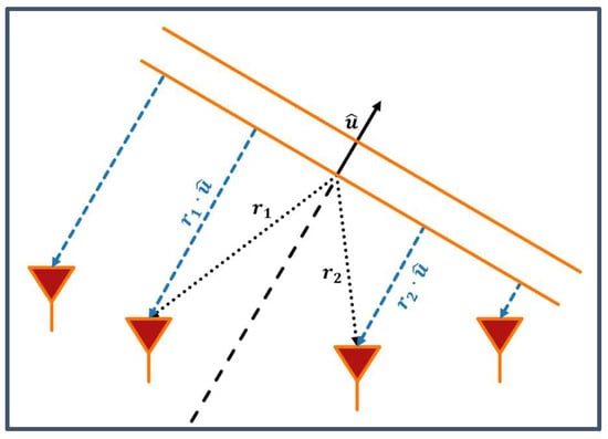
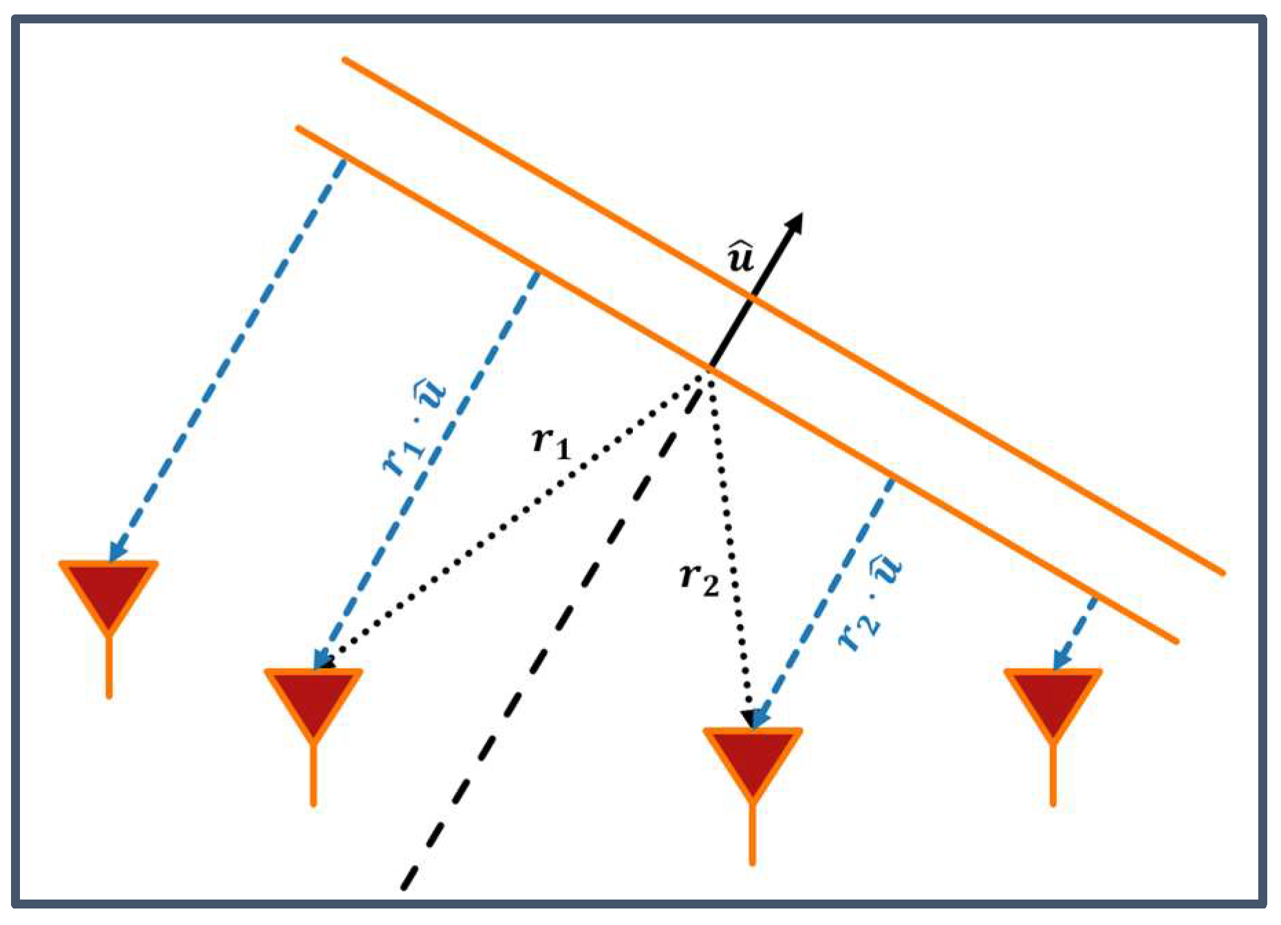
A beamforming algorithm assigns a complex weight to each antenna element, which represents both an attenuation and phase shift [19]. The simplest form of beamforming is conventional beamforming, where all weights are set with a magnitude of one and a phase shift such that all signals constructively interfere in some target direction (. Equation (2) shows the calculation for the weights that satisfy these requirements. These weights form the steering vector (). represents the location of element , represents a unit vector in the target receive direction, and is the wavenumber. Figure 1 gives a visual representation of how a phase shift proportional to results in a coherent phase front in the direction of .
Figure 1.
Illustration of how phase delays proportional to the distance between each element and a plane of constant phase result in a coherent phase front. The orange lines represent planes of constant phase. The blue arrows show the perpendicular distances between each element and a plane of constant phase. The dashed black line shows the direction of travel of the wave.
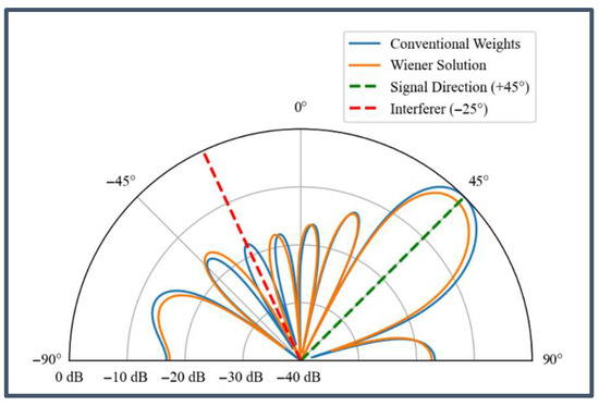
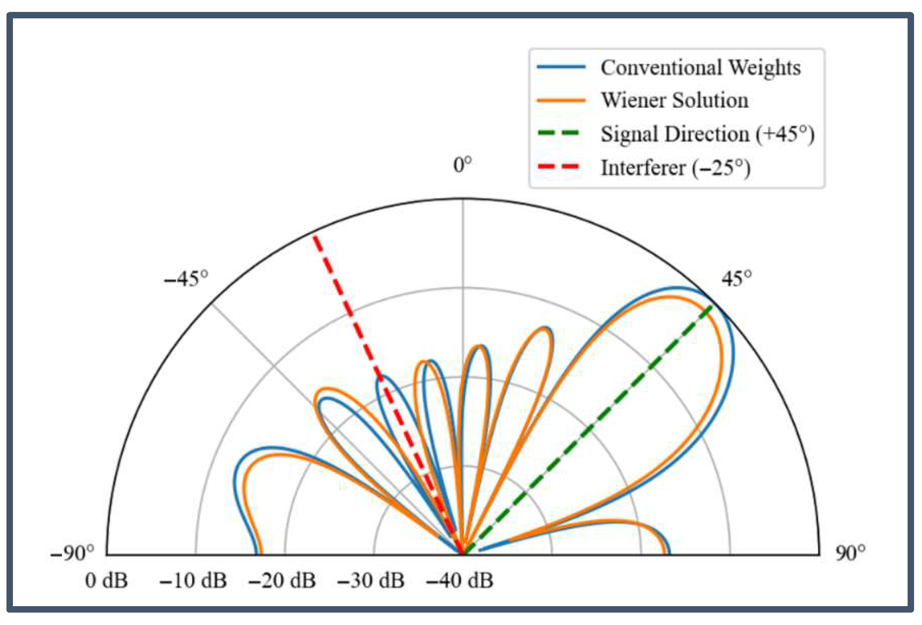
Other beamforming algorithms focus on maximizing SINR by minimizing interfering power rather than only maximizing the signal of interest (SOI) power. The optimal weights for maximizing the SINR form the Wiener solution (Equation (3)) [19] (pp. 945–959). is the inverse of the covariance of the input matrix () and is the cross correlation between and the target signal (). Figure 2 shows array gain patterns using both conventional beamforming weights, where the gain in the direction of the SOI is maximized, and the Wiener solution weights where SINR is maximized. In Figure 2, conventional beamforming results in a gain in the direction of the SOI that is 17 dB higher than the gain in the direction of the interferer. With the Wiener solution weights, the gain in the direction of the SOI is 39 dB higher than the gain in the direction of the interferer, which will result in a higher SINR.
Figure 2.
Array gain pattern using conventional beamforming (blue) and the Weiner solution (orange). The green line represents the signal of interest (SOI) and the red line represents an interferer. The Wiener solution results in a larger difference between the gain in the direction of the SOI and the gain in the direction of the interferer than conventional beamforming (39 dB vs. 17 dB).
Two methods of calculating the Weiner solution weights exist. First is minimum mean squared error (MMSE) beamforming, where the value of the SOI at each sample in time is known. MMSE beamforming sets the weights to minimize the average square difference between the target signal and the output of the array (Equation (4)). Solving Equation (4) yields Equation (3). Using MMSE beamforming requires knowledge of the target value of the SOI at each sample in time. In practice, this works through first transmitting a known header waveform for the beamformer to use to converge on the optimal weights, then sending data after the weights have been set.
The second method of calculating the Weiner solution is minimum variance distortionless response (MVDR) beamforming. MVDR beamforming works by constraining the weights to have a non-zero gain in a target direction while minimizing the total power received by the array. Equation (5) gives the formula for calculating the optimal weights using MVDR beamforming. Averaged over infinite samples, Equations (5) and (3) are identical and both result in the Wiener solution [4]. MVDR beamforming does not require knowledge of the SOI, but it does require knowledge of the steering vector (), which requires knowing the position of each element and the angle of arrival of the SOI (Equation (2)).
3. Simulated Beamforming with Non-Ideal Random Distributed Arrays
The purpose of these simulations is to determine the effectiveness of conventional, MVDR, and MMSE beamforming when applied to random arrays with non-idealities. The simulated non-idealities include positional error, non-uniform noise powers, and non-uniform element orientations. Simulations measure the SINR of 16-element arrays in the presence of different numbers of interferers. Each interferer has the same power level as the SOI. Unless otherwise specified, each element has an isotropic gain pattern and a noise power of 20 dB below the SOI power. Simulations assume that both the SOI and the interferers originate in the far-field and are therefore perfect plane waves incident on the array. Simulations ignore multipathing, channel distortion, and interactions between elements. Each simulation represents a snapshot in time of a motion-dynamic UAV swarm. These assumptions are made to provide a simple comparison between beamforming algorithms that could later be adapted to more specific environments with multipathing or moving elements. The goal of this paper is to strictly examine beamforming in the presence of the non-idealities listed above.
Both MMSE and MVDR beamforming calculate weights that seek to undo the effects of the communication channel and outside interference. If UAVs move quickly enough, the channel changes during the course of a single packet transmission, which invalidates the assumptions made in these simulations. Without future work, the results of these simulations can only be applied to swarms in which each element only moves a small fraction of a wavelength over the course of a transmission.
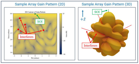
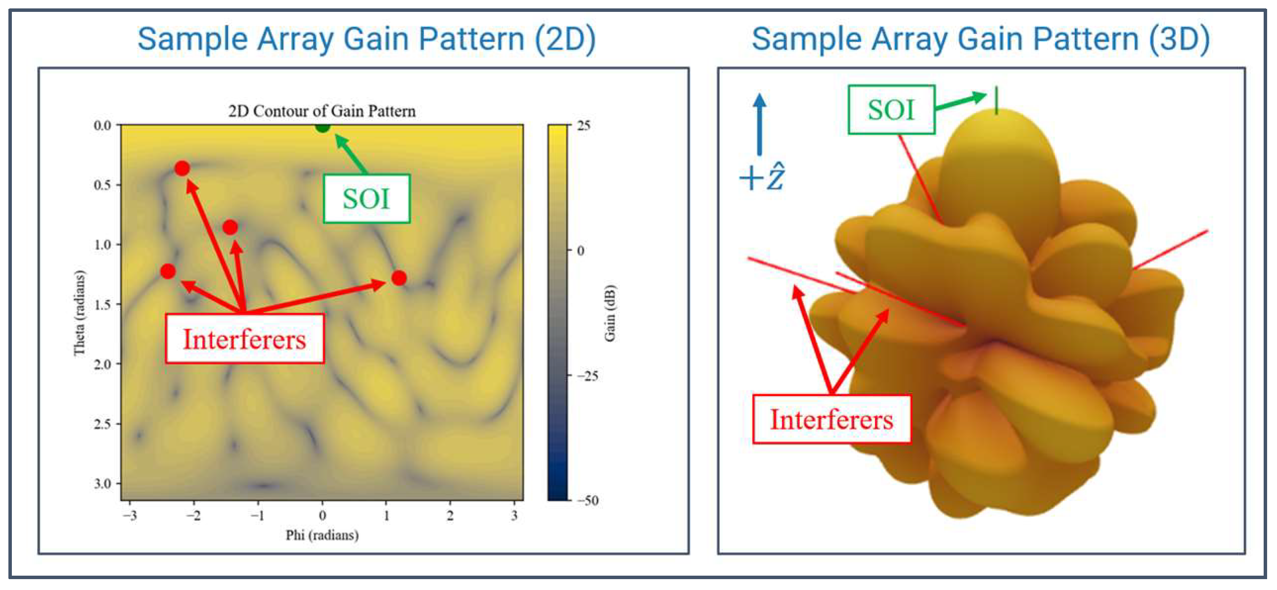
Campbell shows that MMSE beamforming works with ideal random arrays and places nulls in the direction of interferers [4], and the simulations designed for this paper confirm this finding. Figure 3 shows an example of this paper’s simulations using MMSE beamforming to null out four interferers using an ideal 16-element random array.
Figure 3.
Minimum mean squared error (MMSE) beamforming with a 16-element random array, resulting in high gain in the direction of the SOI and low gain in the directions of interferers. The heatmap on the (left) is a 2D projection of the 3D gain pattern on the (right). Red lines represent the directions of arrival of the interferers and the green line represents the SOI.
3.1. Imperfect Localization
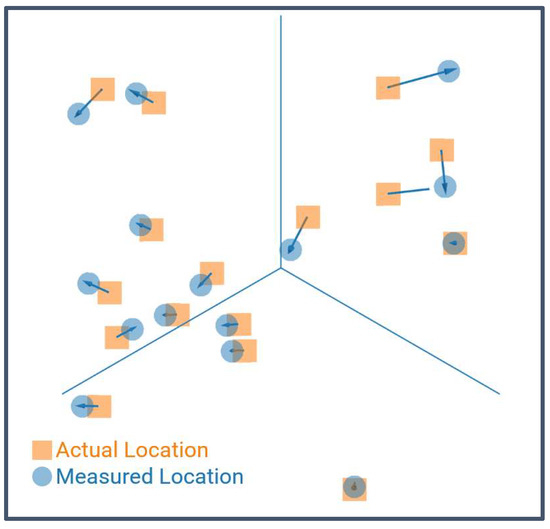
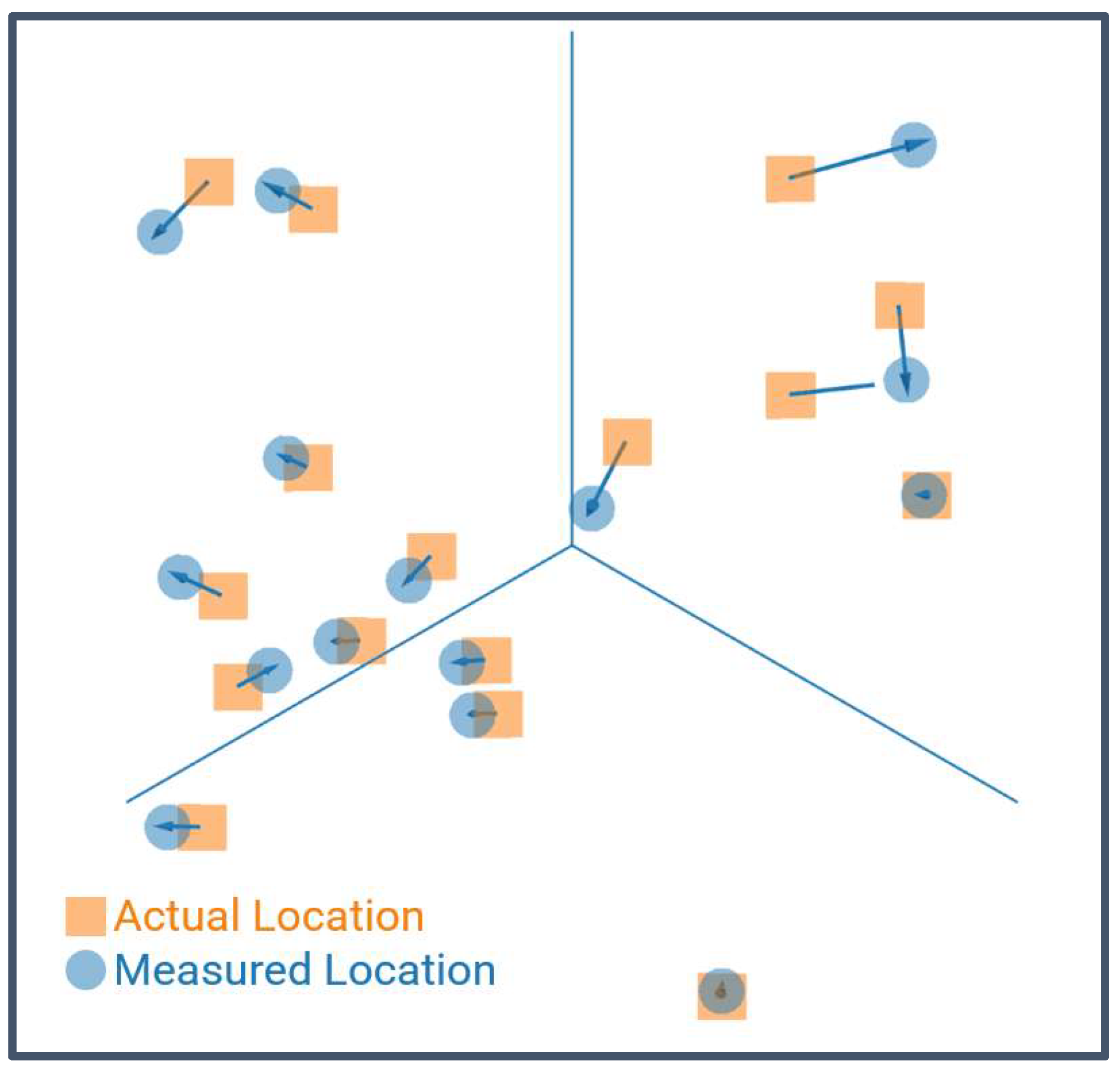
This simulation assigns each element a measurement error vector in a random direction in 3D space. The magnitudes of the errors follow a normal distribution with a mean of zero and a standard deviation of . The element location fed to the beamforming algorithms is the actual element location plus the error vector (Figure 4).
Figure 4.
Measurement error for a 16-element random array. The orange squares show the actual location of each element. The blue circles show the location fed to the beamformers.
Simulations measure SINR for various aperture sizes, numbers of interferers, and positional error standard deviation () for both conventional and MVDR beamforming. Localization error simulations do not include MMSE beamforming since MMSE beamforming does not require knowledge of the position of each element and is therefore unaffected by localization error. Additionally, MVDR beamforming becomes more robust to steering vector error through the use of diagonal loading [20,21,22]. Equation (6) gives the calculation of MVDR weights with diagonal loading, where is the identity matrix and is a constant that can be tuned for optimal robustness. Simulations include various values for from zero (normal MVDR weights) to (conventional beamforming weights).
3.2. Non-Uniform Noise Powers
This simulation assigns each element a noise power relative to the received power of the SOI. Element noise powers follow a standard deviation with a mean of 20 dB below the SOI power and a standard deviation of 5 dB.
Equation (7) shows the calculation for the signal-to-noise-ratio (SNR) of an array with no interference. Solving for the optimal weight magnitudes that maximize yields Equation (8). Equation (8) states that if an element has an SNR -times lower than another element, it should be assigned a weight magnitude that is -times lower than the other element in order to maximize the array output SNR. This simulation examines whether the magnitudes of the weights assigned using MMSE beamforming with non-uniform element SNRs agree with Equation (8) and therefore maximize array SNR.
Equation (8) implies that conventional beamforming never achieves maximum array SNR in the presence of non-uniform element SNRs since the magnitudes of all weights in conventional beamforming are equal.
3.3. Non-Uniform Element Orientations
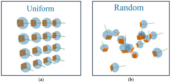
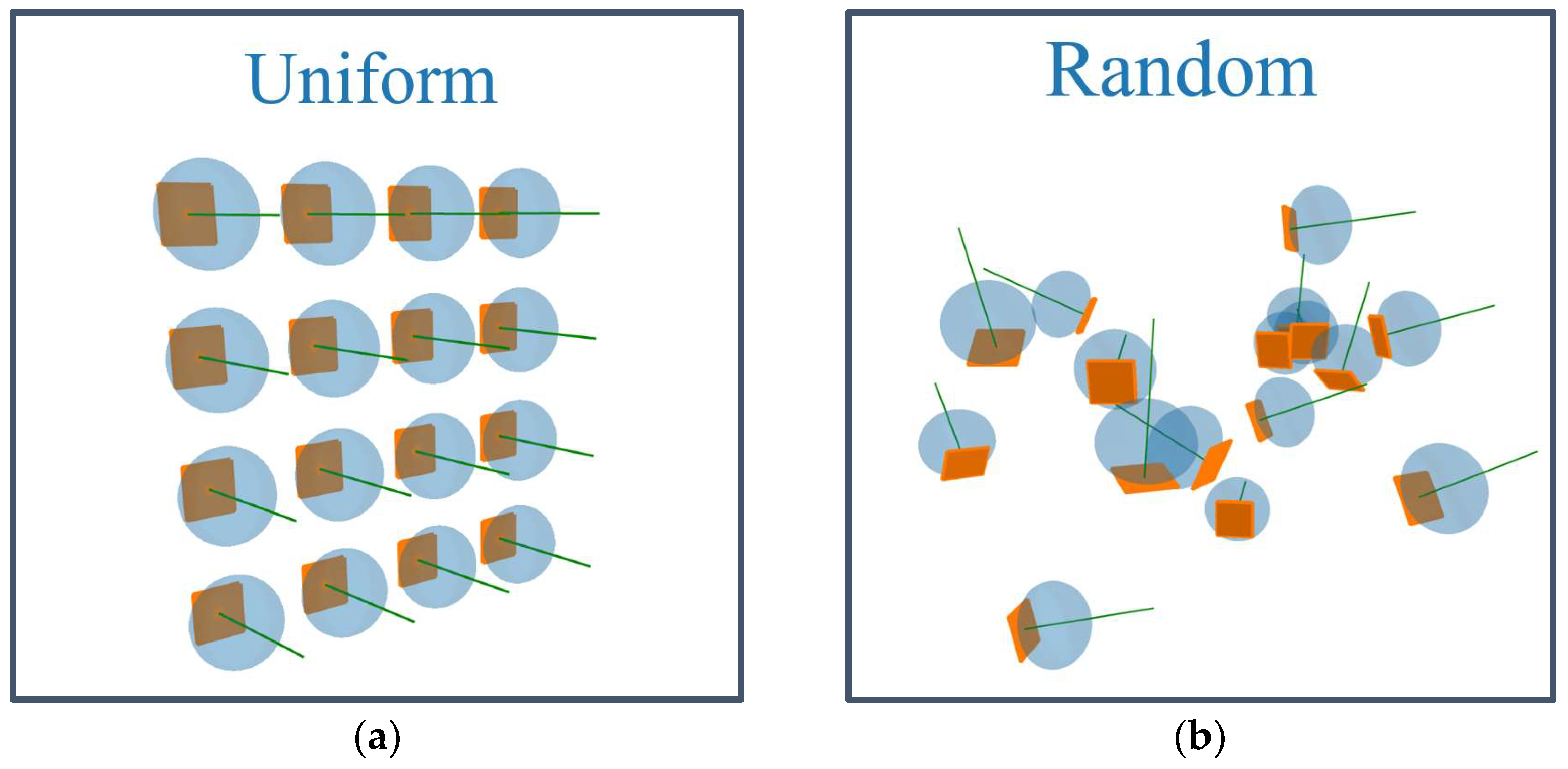
This simulation assigns all elements a gain pattern defined by where is the angle between the element’s broadside direction and the direction in which the gain is measured. The simulation assigns all elements a random broadside direction that is within of the angle of arrival of the SOI. Figure 5 gives a comparison between a fixed uniform array, where all elements are oriented in the same direction, and a random array, where all elements are oriented randomly. Randomly oriented elements have non-uniform gains in the directions of the SOI and interferers.
Figure 5.
Comparison of (a) uniform and (b) non-uniform arrays. Orange squares represent patch antennas, the green lines show the broadside directions, and the blue shapes show the gain patterns.
4. Simulated Beamforming Results
4.1. Imperfect Localization
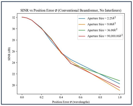
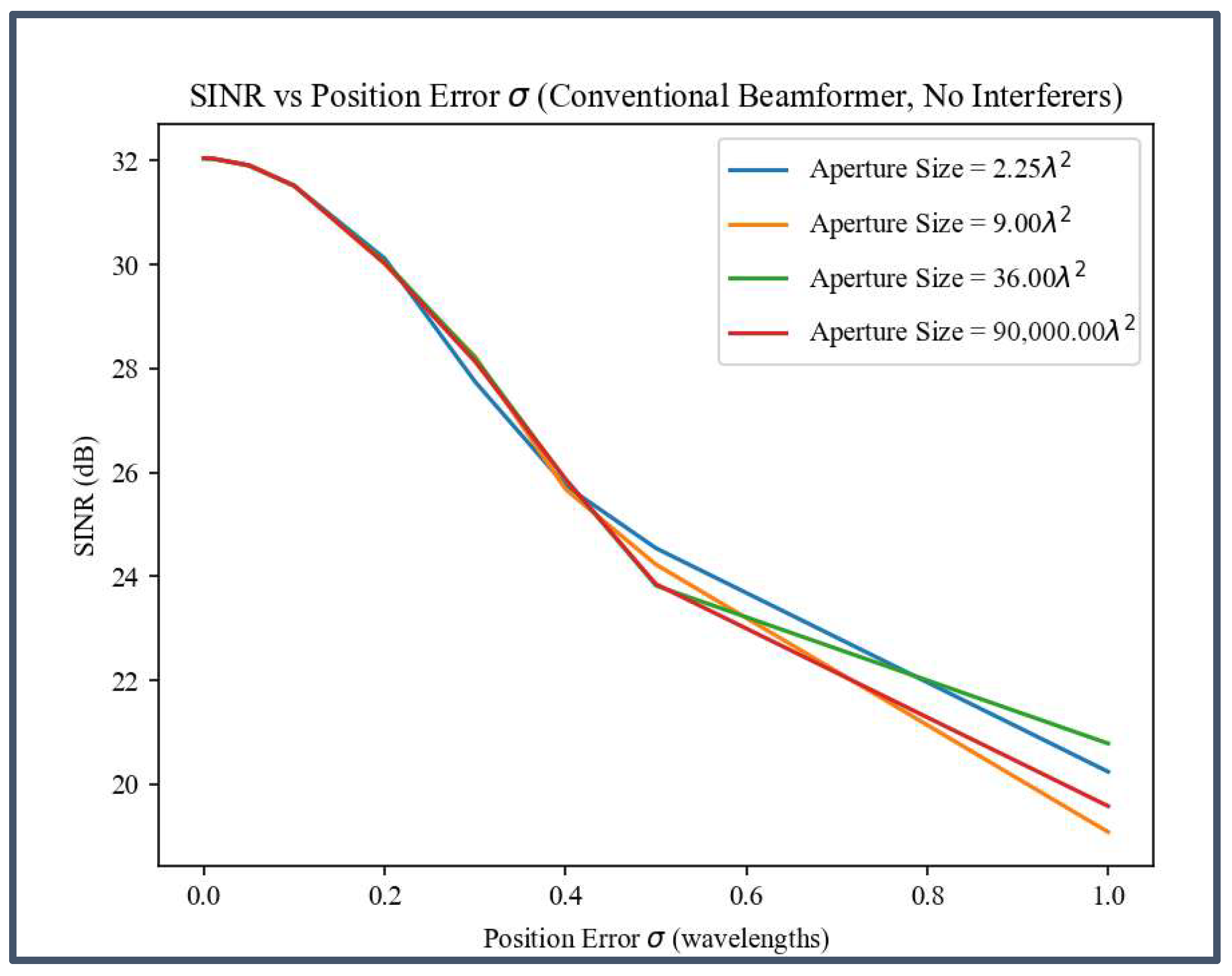
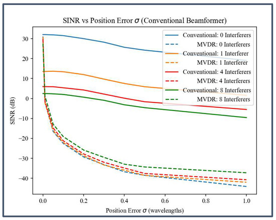
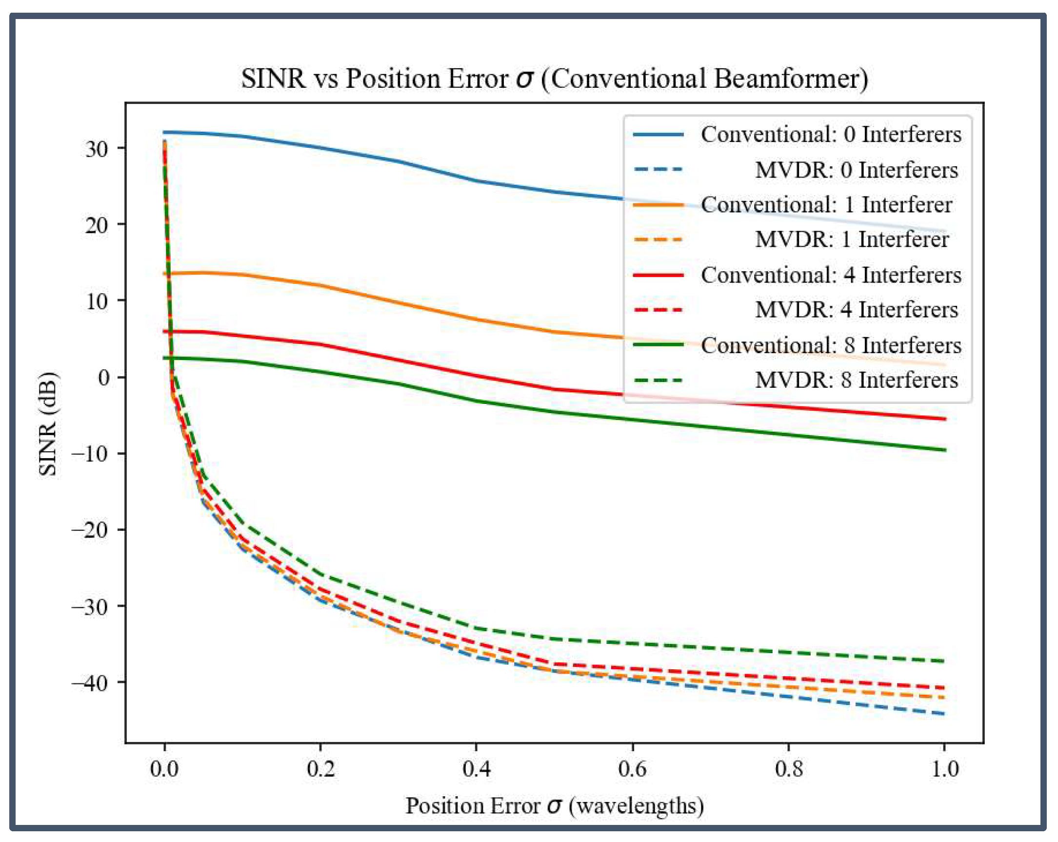
Figure 6 shows simulation results for conventional beamforming with no interferers. A positional error of around 0.25 results in a 3 dB decrease in average output SINR regardless of aperture size. Figure 7 shows the average SINR vs. positional error for both conventional and MVDR beamforming in the presence of various numbers of interferers. Adding interferers decreases the average SINR of conventional beamforming significantly since conventional beamforming does not attempt to null out interferers. MVDR beamforming is relatively unaffected by the presence of interferers when there is no positional error. With positional error introduced, the array SINR decreases significantly. A positional error of only results in a 30 dB decrease in array SINR regardless of the number of interferers.
Figure 6.
Average signal-to-interference-plus-noise ratio (SINR) vs. positional error over 1000 simulated 16-element arrays with various aperture sizes.
Figure 7.
Average SINR vs. positional error over 1000 simulated 16-element random arrays for both conventional and minimum variance distortionless response (MVDR) beamforming with various numbers of interferers. The aperture size is 90,000 to create a very sparse array.
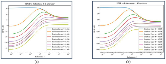
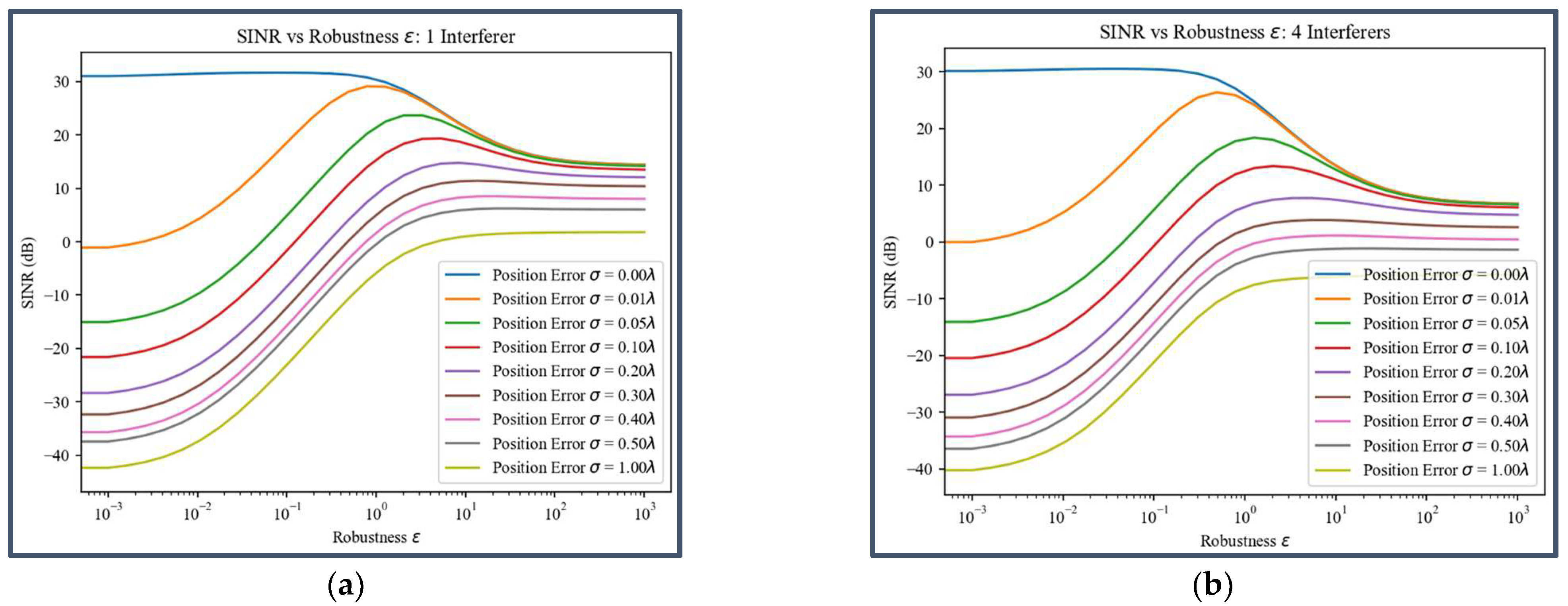
With diagonal loading, MVDR beamforming becomes more robust to localization error (Figure 8). However, even with the ideal value of , positional error significantly reduces array SINR. For a positional error of 0.01 (orange lines), the maximum achievable SINR with 1 interferer is 29.1 dB and with 4 interferers is 26.4 dB. These correspond to a 2.5 dB and 4.1 dB decrease in SINR compared to the case with no positional error. If the positional error increases to 0.05, then the maximum achievable SINR with 1 interferer is 23.7 dB and with 4 interferers is 18.4 dB. These correspond to a 7.9 dB and 12.1 dB decrease in SINR compared to the case with no positional error. For S-Band frequencies, a positional error of 0.01 corresponds to errors of a few millimeters, and for K-Band frequencies, it corresponds to errors of less than a millimeter. Errors at this scale are inevitable in many distributed array applications. This implies that MVDR beamforming is not ideal for distributed array applications.
Figure 8.
Average SNIR vs. for various positional error s with (a) 1 interferer and (b) 4 interferers. These simulations use robust MVDR beamforming and sparse 16-element random arrays.
4.2. Non-Uniform Noise Powers
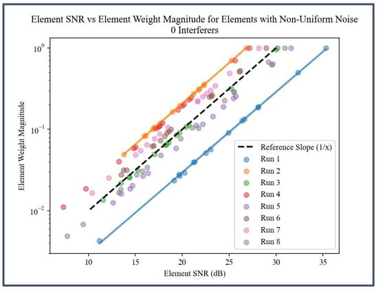
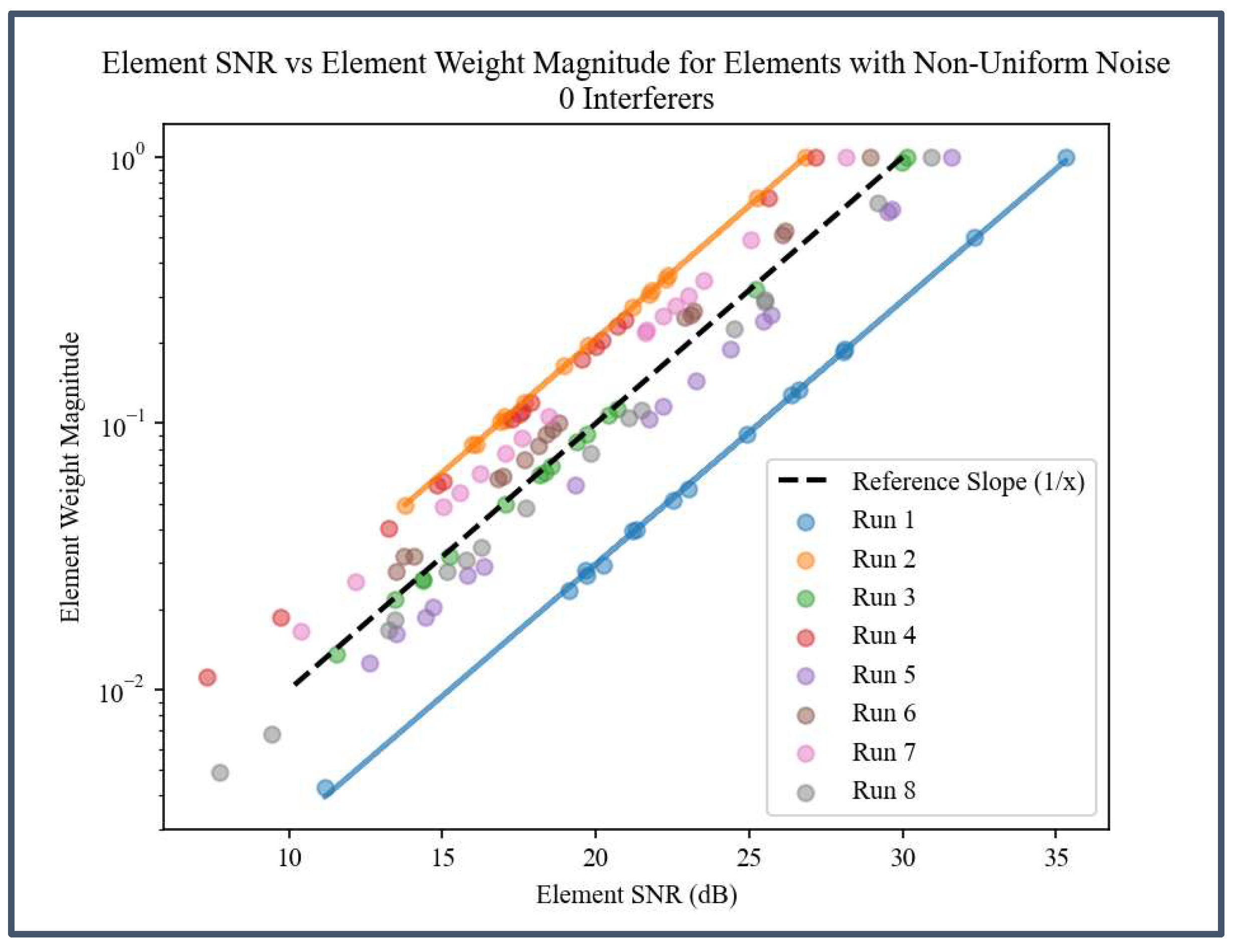
Figure 9 shows the results of eight representative simulations of MMSE beamforming with 16-element random arrays with non-uniform noise and no interferers. The average correlation between element SNR and assigned weight magnitude over 200 simulations is 0.9999. This shows that MMSE beamforming assigns the ideal weights for maximizing array SNR as defined in Equation (8).
Figure 9.
Plot of 8 representative simulations of sparse 16-element random arrays with no interferers. Each point shows the signal-to-noise ratio (SNR) of an element and the magnitude of the weight assigned to that element. The blue and orange lines are linear regression lines for runs 1 and 2 respectively.
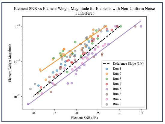
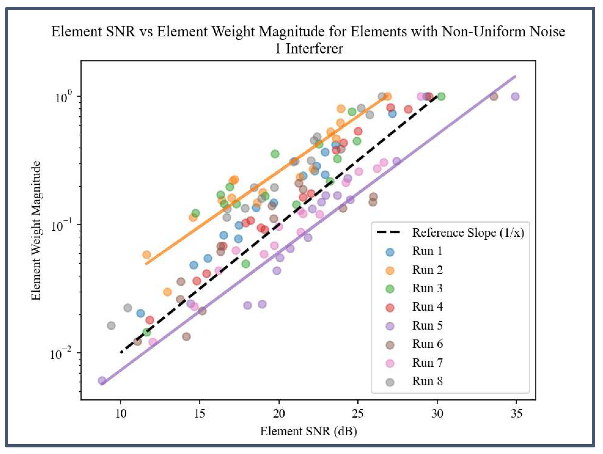
With the addition of an interferer (Figure 10), the average correlation between element SNR and assigned weight magnitude over 200 simulations drops to 0.9607. This occurs because maximizing array SINR requires both placing a null in the direction of the interferer as well as assigning higher weight magnitudes to less noisy elements.
Figure 10.
Plot of 8 representative simulations of 16-element random arrays with one interferer. Each point shows the SNR of an element and the magnitude of the weight assigned to that element. The orange and purple lines are linear regression lines for runs 2 and 5 respectively.
Table 1 shows the average correlation coefficient and average array SINR for various numbers of interferers. As the number of interferers increases, the average correlation coefficient decreases. Nulling out interferers becomes more important for maximizing SINR than assigning higher weight magnitudes to less noisy elements. The average array SINR only decreases 5.86 dB with the addition of eight interferers. This shows MMSE beamforming nulls out interference and maximizes array SINR even with non-uniform noise powers.
Table 1.
Average output SINR and correlation coefficient between element SNR and assigned weight magnitude over 200 simulations for each number of interferers.
4.3. Non-Uniform Element Orientations
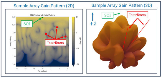
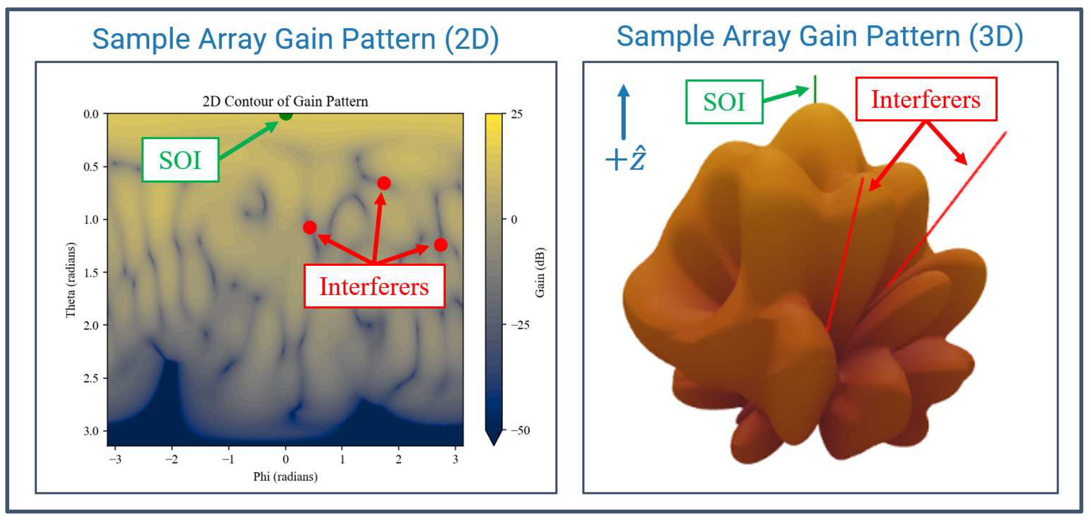
Figure 11 shows a representative sample of a 2D and 3D array gain pattern of a 16-element random array using MMSE beamforming with elements oriented in random directions. Elements have gain patterns and point within of the angle of arrival of the SOI (), so the gain in in the direction is low.
Figure 11.
Representative sample of a 2D and 3D array gain pattern of a 16-element random array with elements oriented in random directions.
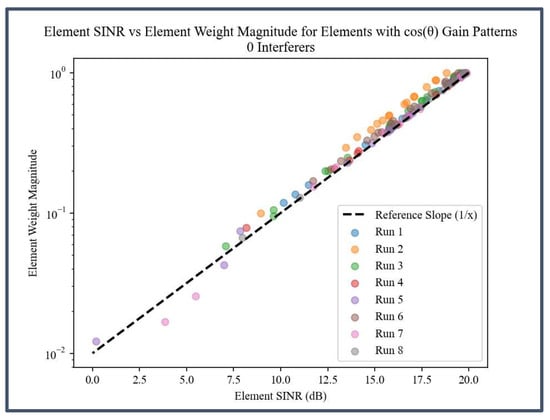
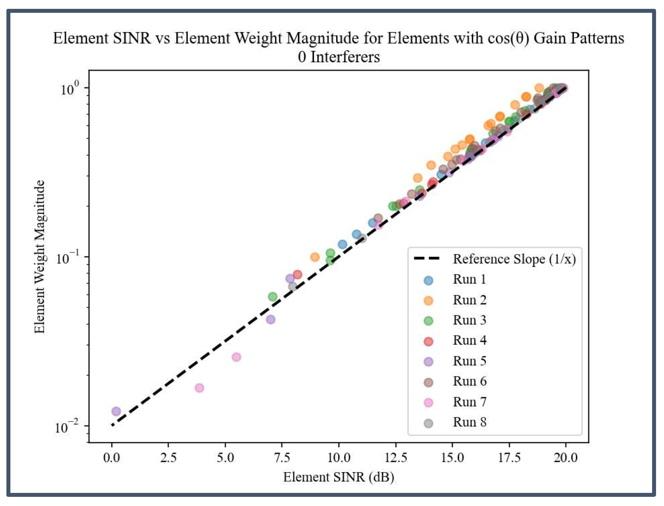
Figure 12 shows the results of eight representative simulations of MMSE beamforming with non-uniform element orientations. Elements that point towards the SOI () have a higher SNR, while elements that point closer to the XY-plane have a lower SNR. Data points closely follow the dashed reference line, which demonstrates that MMSE beamforming assigns the ideal weights for maximizing array SNR as defined in Equation (8).
Figure 12.
Plot of 8 representative simulations of 16-element random arrays with non-uniform element orientations and no interferers. Each point shows the SNR of an element and the magnitude of the weight assigned to that element.
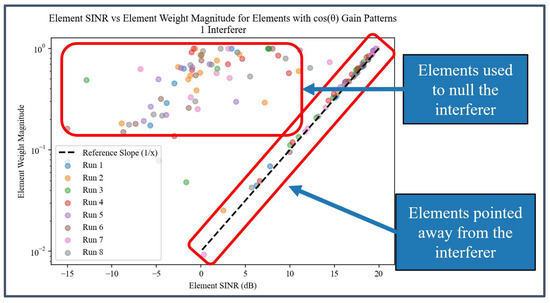
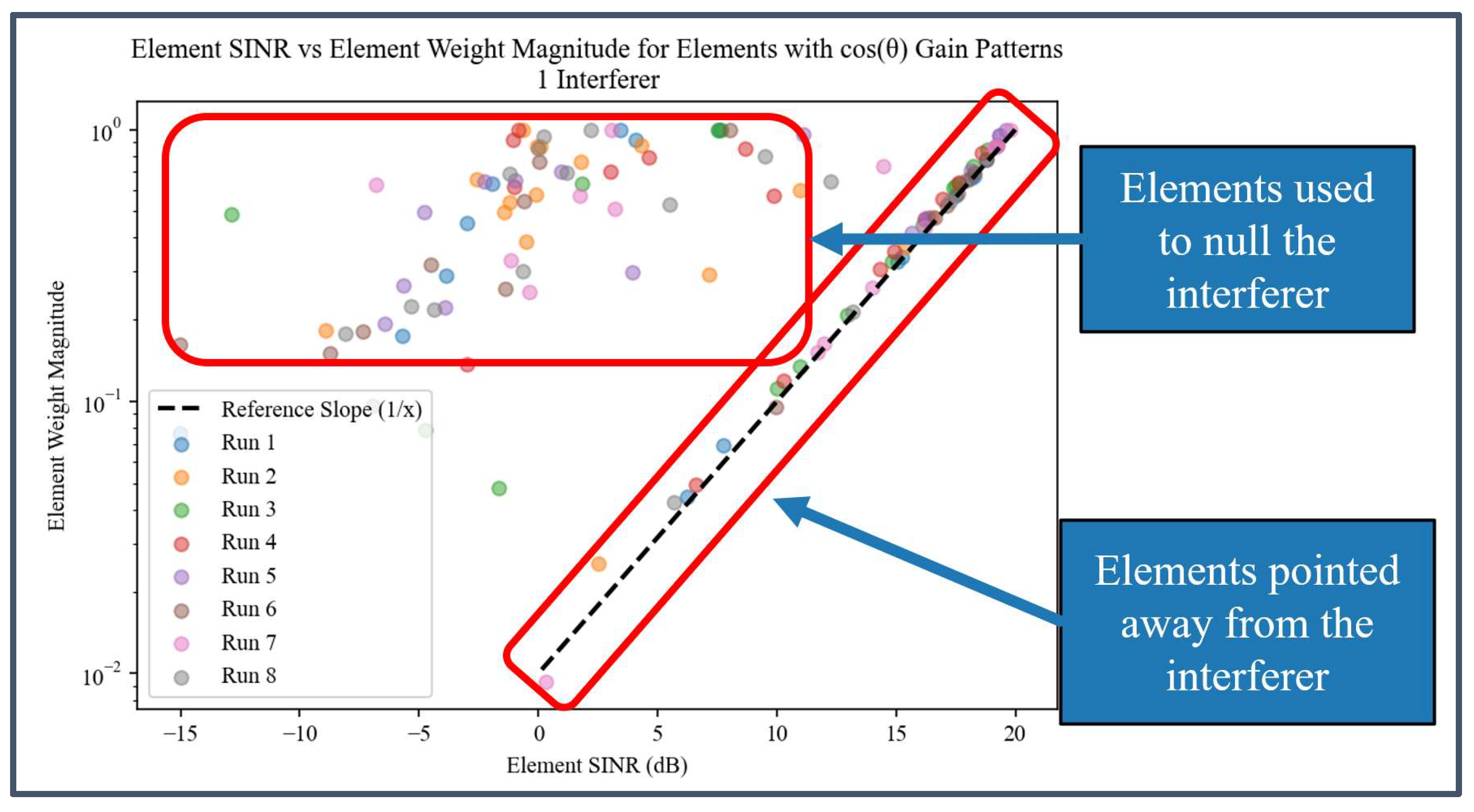
With the addition of an interferer (Figure 13), elements divide into two categories. Elements pointed away from the interferer continue to follow the trend given in Equation (8). Elements pointed toward the interferer have a higher weight magnitude than predicted by Equation (8) in order to null out the interferer. Those elements do not fit well on the reference line. Table 2 shows that the average array SINR only decreases 3.54 dB with the addition of 8 interferers, demonstrating that MMSE beamforming nulls out interfering signals and maximizes array SINR even in the presence of non-uniform element orientations.
Figure 13.
Plot of 8 representative simulations of 16-element random arrays with non-uniform element orientations and one interferer. Each point shows the SNR of an element and the magnitude of the weight assigned to that element.
Table 2.
Average output SINR with non-uniform element orientations over 200 simulations for each number of interferers.
5. Demonstrating MMSE Beamforming with an Experimental Random Array
The goal of this experiment is to demonstrate interference suppression with MMSE beamforming with a real antenna system. The demonstrations use the random volumetric array Medusa testbed [4]. Stationary elements represent the location of a motion-dynamic UAV swarm during a single snapshot in time. Between measurements, the location of each element changes to represent the motion of the UAV swarm. These experiments show interference suppression without knowledge of the location of each element and with non-ideal elements.
5.1. Setup
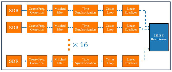
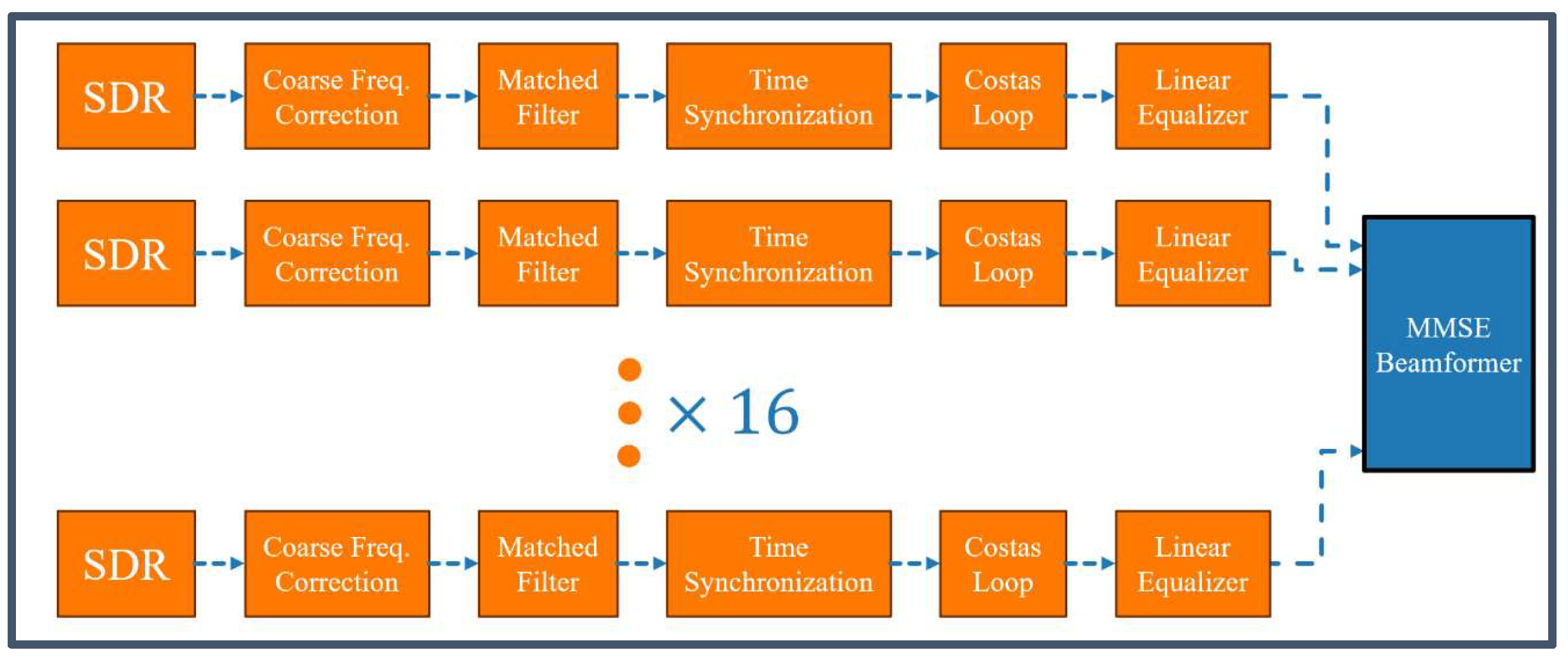
The experiment setup consists of two transmitting antennas. One transmits a known binary phase shift key (BPSK) waveform while the other transmits random gaussian noise as an interferer. Each of the 16 channels on Medusa decodes the BPSK waveform and measures the SINR of that specific antenna element. The decoding process consists of course frequency correction, a matched filter, Miller–Meuler time synchronization, a Costas loop, and a linear equalizer [23] (Figure 14). The samples from each channel are the inputs to an MMSE beamformer.
Figure 14.
Block diagram of Medusa receiver architecture. Samples from each channel’s software-defined radio (SDR) are filtered and corrected for phase and frequency offsets then fed into an MMSE beamformer.
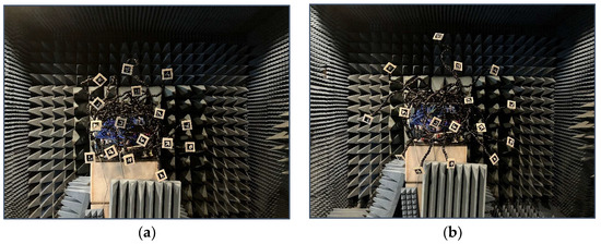
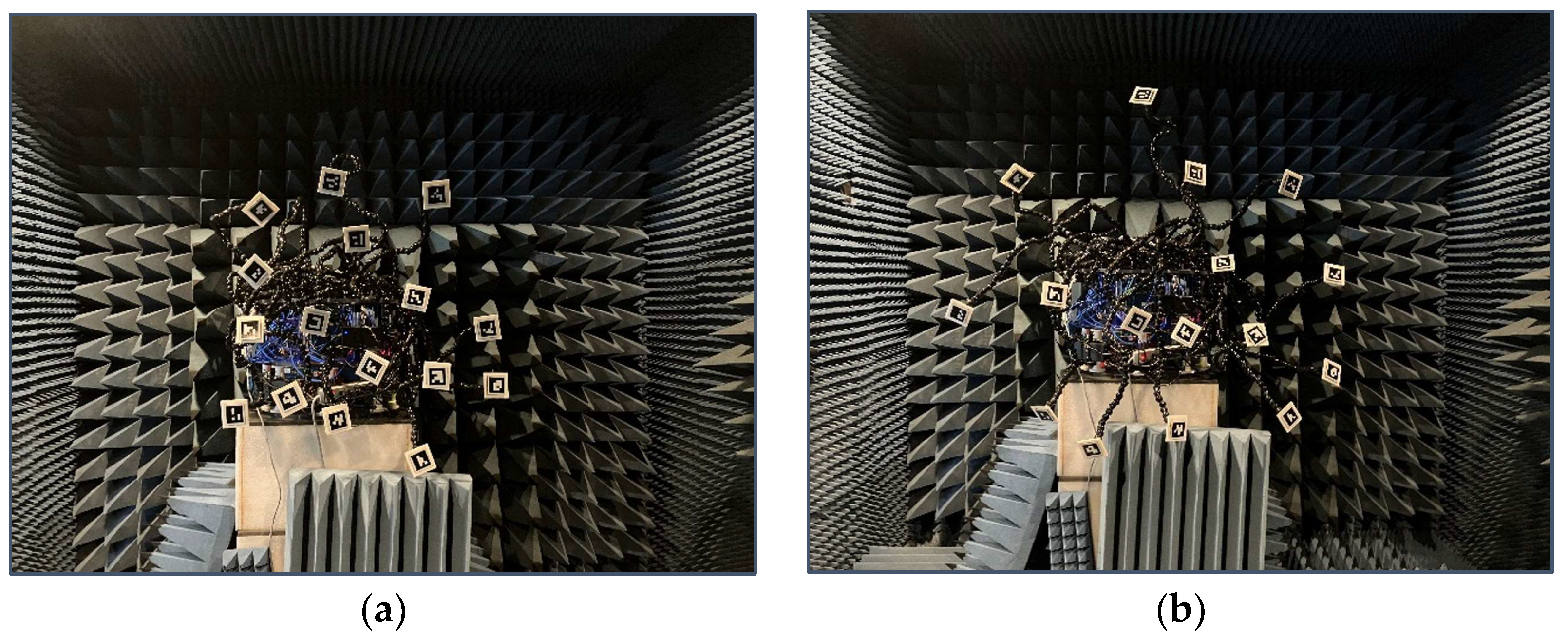
The following sections include data from a variety of configurations of Medusa with different aperture sizes and element rotations. Aperture size configurations include “small aperture” (around 1 m diameter) and “large aperture” (around 1.5 m diameter). Figure 15 shows Medusa in both of these configurations. Element rotation configurations include “broadside” (all elements broadside to the target antenna) and “tilted” (all elements randomly angled within 45 degrees of broadside to the target antenna).
Figure 15.
(a) Medusa in “small aperture” configuration; (b) Medusa in “large aperture” configuration.
Each measurement consists of the following steps:
- Randomize the position of each antenna element according to the configuration used for that measurement (small vs. large aperture and tilted vs. broadside rotation).
- Turn on the SOI, capture samples, and record SINR of each element.
- Calculate weights using MMSE beamforming and record array SINR.
- Turn on the interferer and SOI, capture samples, and record SINR of each element.
- Record array SINR without changing weights from step 3.
- Update weights using MMSE beamforming and record array SINR.
The results compare the array SINR to the maximum possible SINR given the SINR of each channel and assuming that all noise is gaussian and uncorrelated between channels. Equation (9) shows the calculation of the maximum SNR assuming all noise is uncorrelated. Equation (9) derives from using the weights given by Equation (8).
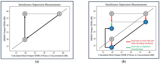
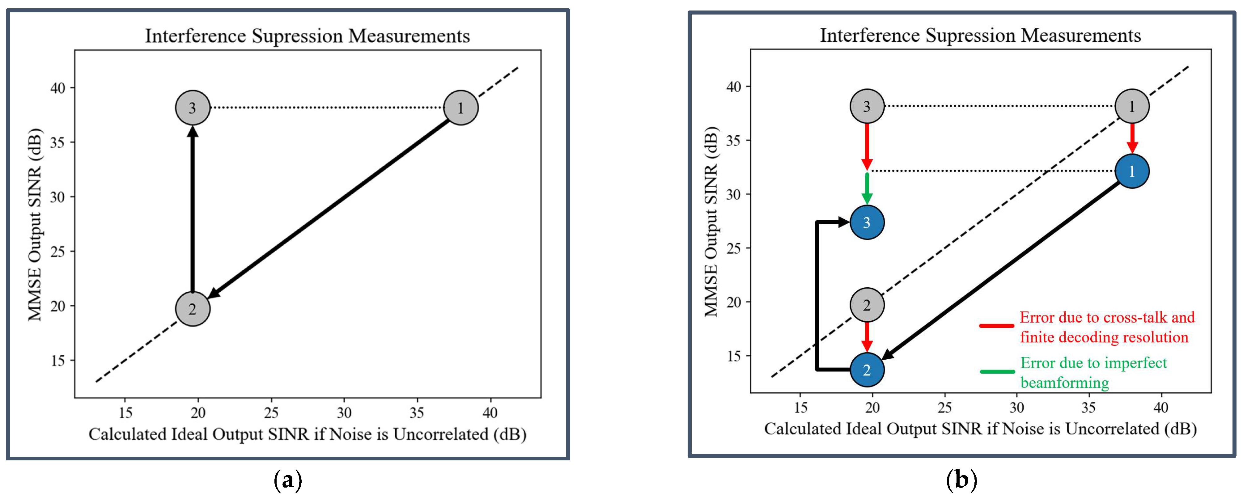
Figure 16a shows the ideal results for the data points described above. Bubble 1 shows the ideal datapoints with the SOI on and the interferer off. In this case, all noise is gaussian and uncorrelated, so measurements fall along the dashed black line. With the interferer on and the weights unchanged, the noise on each channel will increase and measurements fall in Bubble 2. With the weights recalculated to null out the interferer, the measurements fall in Bubble 3. The increase in output SINR from Bubble 2 to Bubble 3 is measured as . The dotted black line shows that the array SINR in Bubble 1 and Bubble 3 are equal. While the interferer adds more noise to each individual channel, it has no effect on the array SINR if it is perfectly nulled out. The difference in output SINR from Bubble 1 to Bubble 3 is measured as and is ideally equal to 0 dB.
Figure 16.
(a) Ideal locations and (b) expected locations of recorded array SINR vs. ideal array SINR. The gray bubbles represent ideal measurements while the blue bubbles represent the expected measurements. Bubble 1 includes datapoints with the interferer turned off. Bubble 2 includes datapoints with the interference on but weights unchanged. Bubble 3 includes data points with the interferer on and nulled using MMSE beamforming. The dashed line represents points at which the calculated ideal SINR and the MMSE output SINR are equal.
In reality, non-idealities in the Medusa system cause the measurements to not match the ideal locations. The blue bubbles in Figure 16b show the expected measurement locations since Medusa is a non-ideal system. Crosstalk between channels, coupling between antennas, and a finite resolution in the decoding process all cause the array SINR to fall below the ideal value. Imperfect nulling of the interferer causes the array SINR with the interferer on (Bubble 3) to be less than the array SINR with the interferer off (Bubble 1).
5.2. Anechoic Chamber Experiments
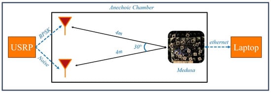
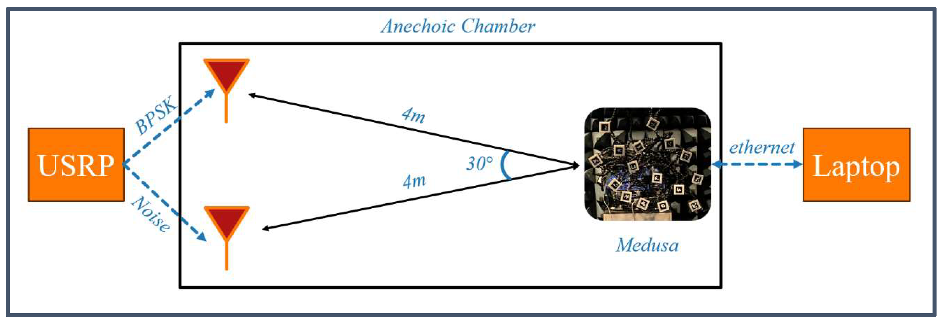
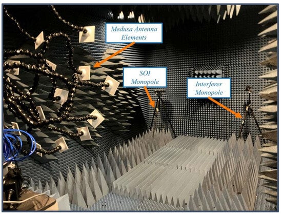
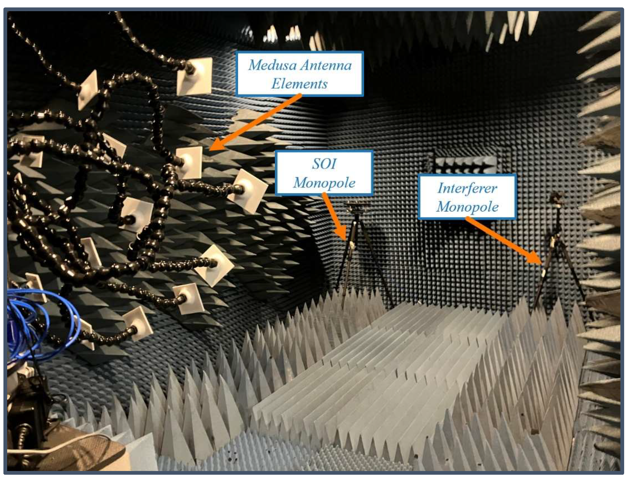
A set of measurements performed inside an anechoic chamber provides a demonstration of successful MMSE beamforming using a non-ideal random volumetric array. Figure 17 provides a diagram of the setup used in this experiment. Figure 18 provides a picture of the test setup.
Figure 17.
Block diagram of Medusa test setup in an anechoic chamber. A Universal Software Radio Peripheral (USRP) from Ettus Research in Santa Clara, CA, USA transmits both the target binary phase shift key (BPSK) signal and random noise as an interferer. The SDRs on Medusa receive the signals and send samples to a computer for processing.
Figure 18.
Medusa test setup in an anechoic chamber. Two monopoles 4 m from Medusa’s antenna elements transmit the SOI and an interfering signal.
The anechoic chamber minimizes outside interference, but other sources of error include the following:
- The monopole antennas are in the far-field compared to each individual antenna on Medusa, but they are in the near-field compared to the size of the array. This means that the waves reaching Medusa have a significant curvature across the face of the array and are not plane waves. This results in phase errors that cause imperfect nulling of the interferer since MMSE beamforming expects phase shifts proportional to the distance from a planar phase front (See Figure 1). Detailed analysis on the effects of near-field curvature on MMSE beamforming is outside the scope of this paper.
- Coupling between elements and crosstalk between channels inside Medusa exist. This results in noise that has some correlation between channels and cannot be suppressed through beamforming.
- The time synchronization and Costas loop have a limited resolution driven by the step sizes programmed into the algorithms. There is a limit to how well they can decode a given signal.
5.3. Uncontrolled Lab Environment Experiments
A set of measurements outside of the anechoic chamber gives a demonstration of mean-squared error beamforming in a non-ideal environment with multipathing, which was not tested in the simulations explained in Section 2. The purpose of this experiment is not to provide rigorous proof that MMSE beamforming works in any environment, but instead to provide a representative demonstration. The channel used in these tests is uncharacterized, so no quantitative conclusions can be made on the effectiveness of MMSE beamforming with random arrays in the presence of multipathing.
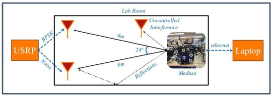
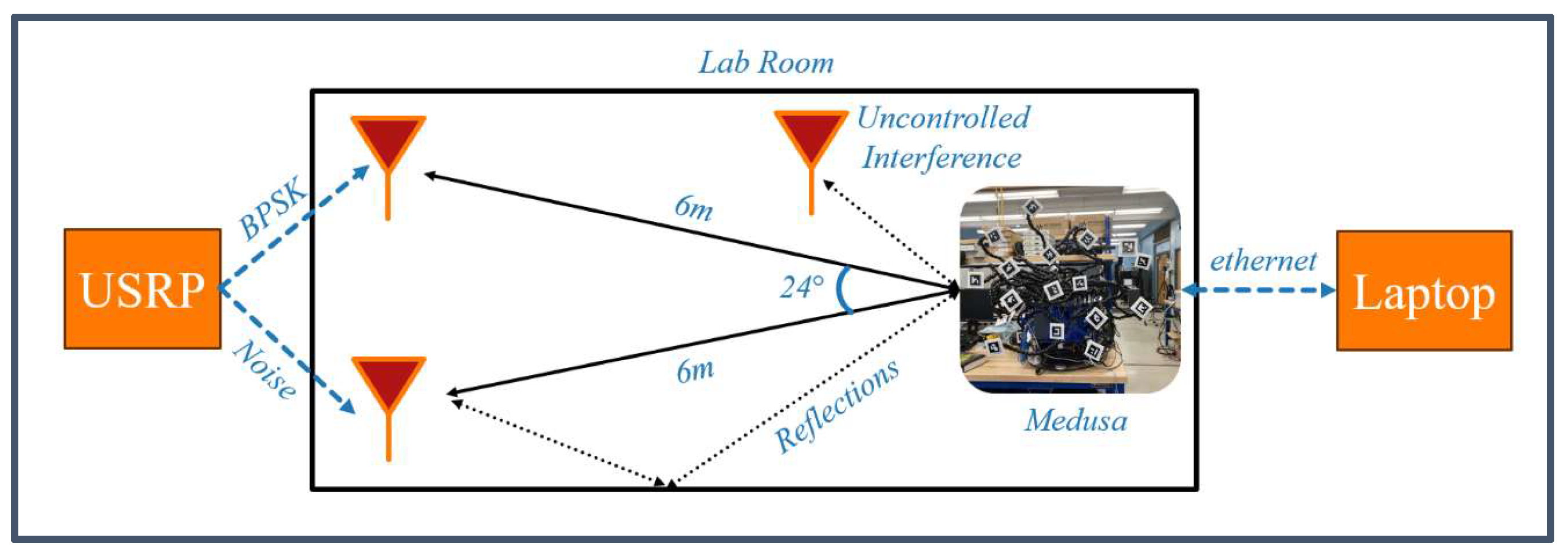
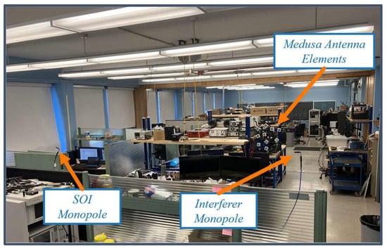
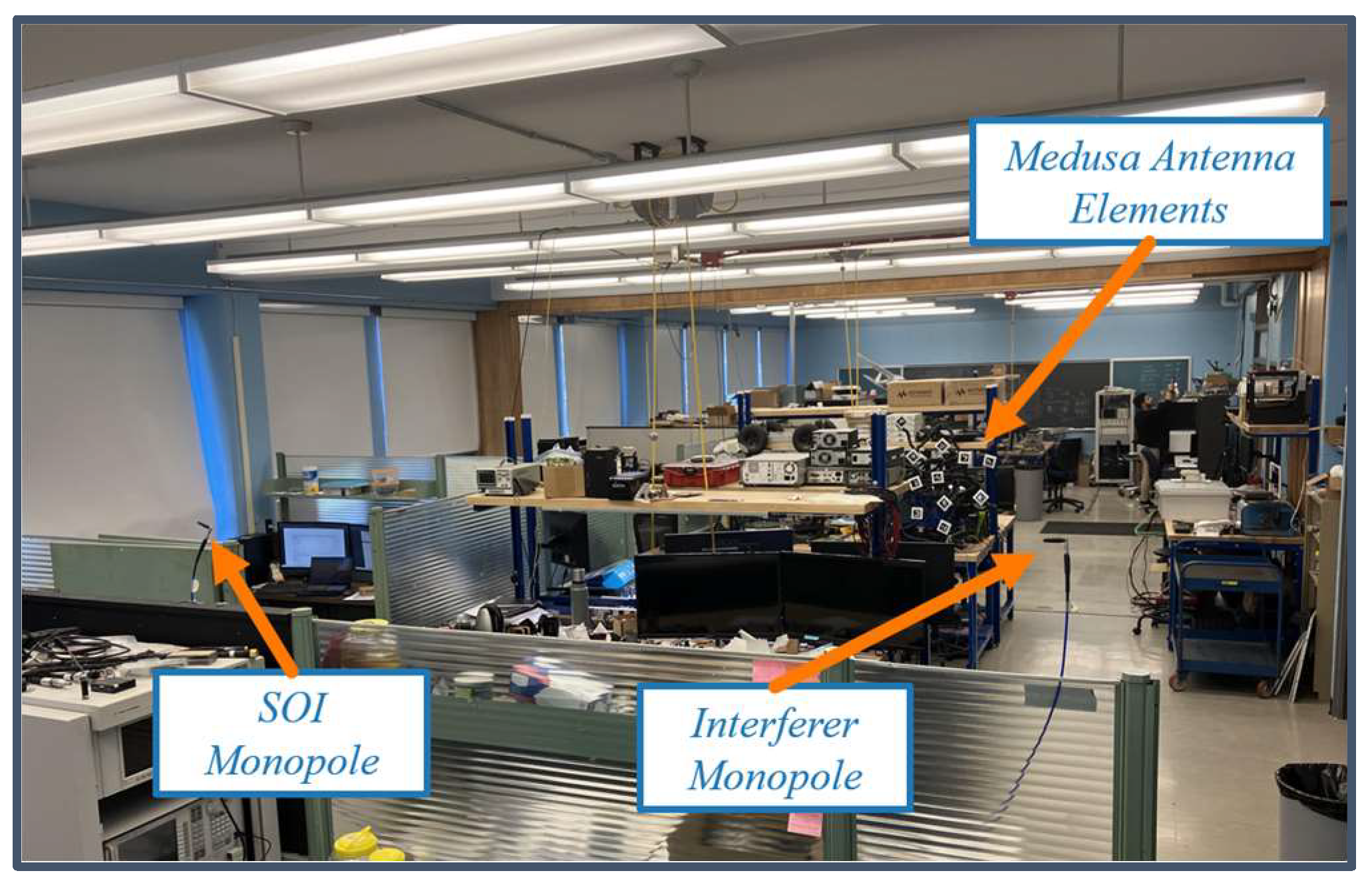
Figure 19 gives a block diagram of the setup in the lab environment. Figure 20 shows a picture of the test setup. The desk between the monopoles and Medusa impedes line of sight communication, and various objects in the room provide surfaces for reflections. Wi-Fi and other systems in the room provide uncontrolled sources of interference.
Figure 19.
Block diagram of Medusa test setup in an uncontrolled lab environment. A USRP transmits both the target BPSK signal and random noise as an interferer. The lab environment creates reflections of both signals as well as uncontrolled interference from other sources. The SDRs on Medusa receive the signals and send samples to a computer for processing.
Figure 20.
Medusa test setup in an uncontrolled lab environment. Two monopoles 6 m from Medusa’s antenna elements transmit the SOI and an interfering signal.
6. Experimental Beamforming Results
Results both in the anechoic chamber and in the lab match the expected results given in Figure 16b. A small sample of twelve measurements for each environment demonstrates interference suppression with non-ideal random arrays. These measurements require a significant amount of time and human resources, as each antenna element must be moved between measurements. A future study with improved automation could provide more statistically rigorous results. The purpose of the measurements taken for this study is only to demonstrate the feasibility of MMSE beamforming with random arrays.
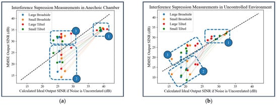
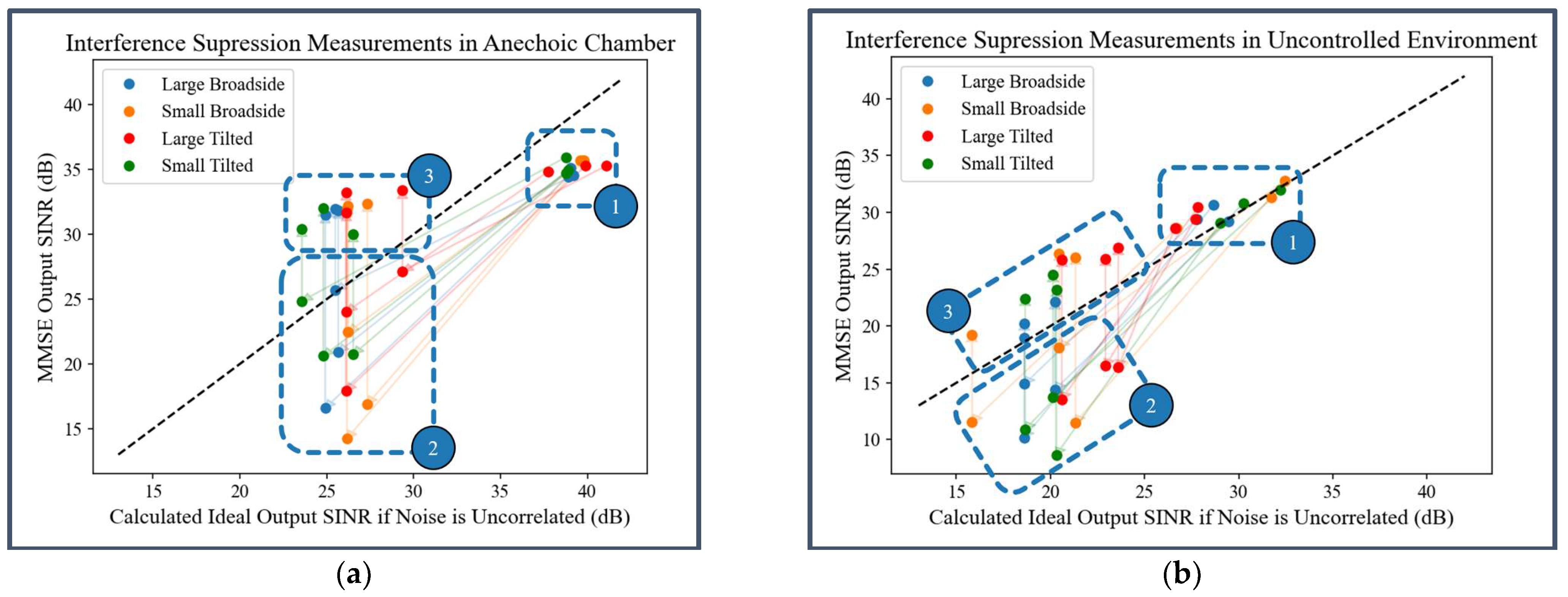
Figure 21a shows the twelve measurements taken within the anechoic chamber. All 12 measurements show an increase in array SINR after the MMSE beamformer recalculates the weights to suppress the interferer (Group 2 to Group 3 in Figure 21a), with the average increase being 10.87 dB (Table 3). Over all twelve measurements, the average decrease between when the interferer is off and when the interferer is nulled is only 3.32 dB (Group 1 to Group 3 in Figure 21a). This shows MMSE beamforming successfully nulls the interferer. Because of the limited number of samples, no statistically significant conclusions can be made to quantify the effectiveness of MMSE beamforming, but the results clearly demonstrate that MMSE beamforming improves the output SINR by partially nulling out the interferer.
Figure 21.
Plot of measurements taken within (a) the anechoic chamber and (b) the uncontrolled lab environment. The x-axis shows the ideal SINR assuming all noise on each channel is uncorrelated. The y-axis shows the measured array SINR. The four distinct colors represent different configurations of Medusa. Group 1 contains datapoints with no interferer present. Group 2 contains datapoints with the interferer present but the weights unchanged. Group 3 contains datapoints with the weights updated to null out the interferer. Arrows connect data points in the same measurement.
Table 3.
Mean and sample standard deviation of Medusa measurements taken in the anechoic chamber for each configuration, as well as all configurations combined. represents the change in output SINR from when the interferer is on, but not nulled, to when it is nulled using MMSE beamforming. represents the change in output SINR from when the interferer is off to when the interferer is on and nulled.
These results illustrate that MMSE beamforming can null out an interferer without requiring knowledge of element locations and while operating with non-ideal antenna elements. Since the data only includes three measurements in each configuration of Medusa, no conclusive claims about the difference between configurations can be made. A more rigorous future study may provide more detail on how aperture size and element orientation affect interference suppression.
Measurements in the uncontrolled lab environment still show an increase in array SINR after the MMSE beamformer recalculates the weights to suppress the interferer (Group 2 to Group 3 in Figure 21b). However, there is a larger decrease between the array SINR when the interferer is off (Group 1) and the array SINR when the interferer is nulled (Group 3). The mean increased from 3.32 dB in the anechoic chamber to 6.73 dB in the uncontrolled lab environment (Table 4). This indicates that while MMSE beamforming still works, it may become less effective in uncontrolled environments with multipathing. More measurements must be taken to make conclusive statements about the effects of multipathing and uncontrolled interference.
Table 4.
Mean and sample standard deviation of Medusa measurements taken in the uncontrolled lab environment for each configuration, as well as all configurations combined. represents the change in output SINR from when the interferer is on, but not nulled, to when it is nulled using MMSE beamforming. represents the change in output SINR from when the interferer is off to when the interferer is on and nulled.
Unlike in Figure 21a, some of the measurements in Group 1 of Figure 21b lie above the dashed black line, meaning that the array SINR is higher than the calculated ideal SINR if all noise is uncorrelated. This indicates that some noise seen by the elements in Medusa is correlated and caused by an uncontrolled interferer. This confirms that the lab contains sources of interference other than the intentional interferer, and MMSE beamforming suppresses them.
7. Discussion
This paper focused on determining the feasibility of various adaptive beamforming algorithms for use in real distributed array applications. Simulations showed that MVDR beamforming degrades significantly when the localization error is on the order of . MMSE beamforming works to maximize array SINR and is robust to localization error and non-uniform elements. This is due to the fact that MMSE beamforming seeks to minimize the error between the received signal and the known target signal. By finding weights that minimize that error, MMSE beamforming estimates the transmission channel and accounts for any phase and gain errors caused by localization errors and non-uniform elements. MMSE beamforming provides strong interference suppression as long as the channel estimates update quickly enough to account for changes in the channel as elements move. MVDR beamforming, on the other hand, seeks to maximize gain in a target direction given perfect knowledge of the location and gain pattern of all elements. If there are errors in those inputs, the interference suppression will decrease.
However, MMSE beamforming requires transmitting a known header waveform for calculating array weights. This means that MMSE beamforming requires the transmitter and receiver to agree on a pre-determined header waveform, and it results in lower data rates as some portion of the transmission must be used for the header waveform. Future work needs to be done on optimizing the structure and length of header waveforms for distributed array applications. MMSE beamforming also significantly reduces the complexity of distributed swarm array applications since it does not require measuring the location of each element.
Experiments with the Medusa random array testbed confirmed that MMSE beamforming suppresses interference under real-world hardware and channel conditions. MMSE beamforming demonstrated interference suppression in both an anechoic chamber and an uncontrolled lab environment. These experiments represent the first real-world demonstrations of digital beamforming with a random volumetric array to suppress interfering signals.
Previous work suggests that in an environment with no interferers, approximately equal element SNRs, and localization error on the order of , conventional beamforming works well for both transmitting and receiving signals [1,18]. MMSE beamforming should only be used in swarming applications where the above conditions are not true, as it adds the extra complexity of a header waveform.
Areas for future work needed to make motion-dynamic distributed arrays a reality include the following:
- Wireless phase and frequency synchronization between distributed elements.
- Near-field beamforming with random arrays. Many distributed array applications result in targets and interferers in the “near-field” relative to the size of the array.
- Investigation into improvements when using moving elements. This paper assumes that elements are static during each transmission, which may not be a valid assumption for long transmissions or extremely fast elements. When elements move, the transmission channel changes, and weights must be adjusted in order to maintain high gain in the desired direction and interference suppression. Future research will determine if certain beamforming algorithms are more susceptible to small changes in the transmission channel.
- Receiving samples and performing beamforming in real time. The experiments in this paper perform beamforming on samples captured and saved at an earlier point in time.
- Transmission with random distributed arrays. This paper solely focused on adaptive beamforming for receive-based applications.
- Analysis of ideal header waveform, length, and repetition interval for MMSE beamforming.
- Application of other modern robust beamforming algorithms to non-ideal distributed arrays. This paper only examines MMSE and MVDR beamforming.
- Analysis of computation strategies for performing MMSE or MVDR beamforming on computationally constrained UAVs or offloading beamforming calculations to a more capable computer on the ground.
Findings from this paper, along with future work listed above, will serve to make motion-dynamic distributed UAV swarm arrays a reality.
Author Contributions
Conceptualization, R.K., G.H. and B.C.; Methodology, R.K.; Software, R.K., T.B. and B.C.; Validation, R.K.; Formal analysis, R.K.; Investigation, R.K.; Resources, R.K.; Data curation, R.K.; Writing—original draft, R.K.; Writing—review & editing, R.K. and G.H.; Visualization, R.K.; Supervision, G.H.; Project administration, G.H. All authors have read and agreed to the published version of the manuscript.
Funding
This research received no external funding.
Data Availability Statement
The dataset is available on request from the authors.
Conflicts of Interest
The authors declare no conflicts of interest.
Abbreviations
The following abbreviations are used in this manuscript:
| PNT | Position, Navigation, and Timing |
| UAV | Unmanned Aerial Vehicle |
| MVDR | Minimum Variance Distortionless Response |
| MMSE | Minimum Mean Squared Error |
| LMS | Least Mean Squares |
| GNSS | Global Navigation Satellite Systems |
| SINR | Signal to Interference plus Noise Ratio |
| SNR | Signal to Noise Ratio |
| SOI | Signal of Interest |
| SDR | Software Defined Radio |
| USRP | Universal Software Radio Peripheral |
| BPSK | Binary Phase Shift Key |
References
- Harmer, S.W.; Novi, G.D. Distributed Antenna in Drone Swarms: A Feasibility Study. Drones 2023, 7, 126. [Google Scholar] [CrossRef] [Scilit]
- Lo, Y. A Mathematical Theory of Antenna Arrays with Randomly Spaced Elements. IEEE Trans. Antennas Propag. 1964, 12, 257–268. [Google Scholar] [CrossRef] [Scilit]
- Yeh, S.; Chamberland, J.-F.; Huff, G.H. An Investigation of Geolocation-Aware Beamforming Algorithms for Swarming UAVs. In Proceedings of the 2017 IEEE International Symposium on Antennas and Propagation & USNC/URSI National Radio Science Meeting, San Diego, CA, USA, 9–14 July 2017; pp. 641–642. [Google Scholar]
- Campbell, B. Distributed Hybrid Beamforming Techniques for Random Three-Dimensional Arrays. Ph.D. Thesis, The Pennsylvania State University, University Park, PA, USA, 2024. [Google Scholar]
- Buchanan, K.; Wheeland, S.; Manzano-Roth, R.; Loaiza, G.; Sills, M.; Li, J.; Lin, A.; Patefield, M.; Jones, A.; Rodriguez, A.; et al. Final Report Swarm-Enabled Distributed Sensing; NIWC Pacific: San Diego, CA, USA, 2024. [Google Scholar]
- Bu, Y.; Yan, Y.; Yang, Y. Advancement Challenges in UAV Swarm Formation Control: A Comprehensive Review. Drones 2024, 8, 320. [Google Scholar] [CrossRef] [Scilit]
- Phadke, A.; Medrano, F.A. Towards Resilient UAV Swarms—A Breakdown of Resiliency Requirements in UAV Swarms. Drones 2022, 6, 340. [Google Scholar] [CrossRef] [Scilit]
- Sheemar, C.K.; Mahmood, A.; Thomas, C.K.; Alexandropoulos, G.C.; Querol, J.; Chatzinotas, S.; Saad, W. Joint Beamforming and 3D Location Optimization for Multi-User Holographic UAV Communications. IEEE Trans. Commun. 2026, 74, 4974–4988. [Google Scholar] [CrossRef] [Scilit]
- Lin, Z.; Niu, H.; He, Y.; Kang, A.; Zhong, X.; Zheng, C.; Pei, X. Self-Powered Absorptive Reconfigurable Intelligent Surfaces for Securing Satellite-Terrestrial Integrated Networks. China Commun. 2024, 21, 276–291. [Google Scholar]
- Huroon, A.M.; Huang, Y.-C.; Wang, L.-C. Energy-Efficient Transmission Strategy for UAV-RIS 2.0 Assisted Communications Using Rate Splitting Multiple Access. IEEE Trans. Wirel. Commun. 2026, 25, 5246–5261. [Google Scholar] [CrossRef] [Scilit]
- Panicali, A.; Lo, Y. A Probabilistic Approach to Large Circular and Spherical Arrays. IEEE Trans. Antennas Propag. 1969, 17, 514–522. [Google Scholar] [CrossRef]
- Unz, H. Linear Arrays with Arbitrarily Distributed Elements. IRE Trans. Antennas Propag. 1960, 8, 222–223. [Google Scholar] [CrossRef] [Scilit]
- Zhang, X.; Bai, Y.; He, K. On Countermeasures against Cooperative Fly of UAV Swarms. Drones 2023, 7, 172. [Google Scholar] [CrossRef] [Scilit]
- Chen, Z.; Yeh, S.; Chamberland, J.-F.; Huff, G.H. A Sensor-Driven Analysis of Distributed Direction Finding Systems Based on UAV Swarms. Sensors 2019, 19, 2659. [Google Scholar] [CrossRef] [Scilit] [PubMed]
- Yeh, S.-Y. Volumetric Random Phased Arrays and Their Applications. Ph.D. Thesis, A&M University, College Station, TX, USA, 2018. [Google Scholar]
- Jensen, J.S.; Buchanan, K.; Chamberland, J.-F.; Huff, G.H. A Computer Vision-Based Framework for the Synthesis and Analysis of Beamforming Behavior in Swarming Intelligent Systems. In Proceedings of the 2017 IEEE Radar Conference (RadarConf), Seattle, WA, USA, 8–12 June 2017; pp. 118–122. [Google Scholar]
- Zhao, Y.; Li, L.; Hu, D.; Huang, Z.; Guo, X.; Ba, J.; Huang, H.; Yuan, S.; Zhou, J. Positioning Error Analysis of Distributed Random Array Based on Unmanned Aerial Vehicles in Collaborative Jamming. Drones 2025, 9, 234. [Google Scholar] [CrossRef] [Scilit]
- Buchanan, K.; Rockway, J.; Huff, G.H. Random Antenna Array Phase and Range Limitations. In Proceedings of the 2015 IEEE International Symposium on Antennas and Propagation & USNC/URSI National Radio Science Meeting, Vancouver, BC, Canada, 19–24 July 2015; pp. 2499–2500. [Google Scholar]
- Balanis, C.A. Antenna Theory: Analysis and Design, 4th ed.; Wiley: Hoboken, NJ, USA, 2016; ISBN 978-1-118-642060-1. [Google Scholar]
- Cox, H.; Zeskind, R.; Owen, M. Robust Adaptive Beamforming. IEEE Trans. Acoust. Speech Signal Process. 1987, 35, 1365–1376. [Google Scholar] [CrossRef] [Scilit]
- Li, J.; Stoica, P.; Wang, Z. On Robust Capon Beamforming and Diagonal Loading. IEEE Trans. Signal Process. 2003, 51, 1702–1715. [Google Scholar] [CrossRef] [Scilit]
- Yang, L.; Yang, Y.; Yang, J. Robust Adaptive Beamforming for Uniform Linear Arrays with Sensor Gain and Phase Uncertainties. IEEE Access 2019, 7, 2677–2685. [Google Scholar] [CrossRef] [Scilit]
- Litchtman, M. Synchronization | PySDR: A Guide to SDR and DSP Using Python. Available online: https://pysdr.org/content/sync.html (accessed on 9 September 2025).

Disclaimer/Publisher’s Note: The statements, opinions and data contained in all publications are solely those of the individual author(s) and contributor(s) and not of MDPI and/or the editor(s). MDPI and/or the editor(s) disclaim responsibility for any injury to people or property resulting from any ideas, methods, instructions or products referred to in the content. |
© 2026 by the authors. Licensee MDPI, Basel, Switzerland. This article is an open access article distributed under the terms and conditions of the Creative Commons Attribution (CC BY) license.