Physics-Informed Convolutional Neural Network for Localizing and Identifying Rotor Unbalance in the Long-Endurance UAV Turbine Engine

Highlights

What are the main findings?

• The frequency response function (FRF) can achieve robust unbalance localization without requiring a high-fidelity simulation model.
• Compared to pure data-driven or model-based benchmarks, the proposed PICNN achieves higher precision, as demonstrated on an experimental setup representative of the engine installation status on the UAV platform.

What are the implications of the main findings?

• Facing the rotor–stator coupling vibration in most UAV turbine engines, the FRF-based method exhibits its broad engineering practicality because of its flexible requirements for model precision.
• The efficient and physically interpretable method proposed in this paper provides a better tool for UAV turbine engine rotor health monitoring.

Abstract

Various types of turbine engines have been chosen as the primary power source of the long-endurance unmanned aerial vehicles (UAVs) because of their high propulsive efficiency and low specific fuel consumption. To ensure the healthy operation of UAV turbine engines, rotor unbalance should be monitored and constrained to a preset limit. This paper proposes an efficient and physically interpretable method to achieve rotor unbalance monitoring. This method enables the frequency response function (FRF) to inform the neural network design, bringing the physics-informed convolutional neural network (PICNN). Firstly, the FRF gives a qualitative judgment of the axial positions of dominant faulty parts. Then, the following subnet proceeds to achieve quantitative identification. This method is demonstrated on a series of numerical cases and on a twin-disk rotor-bearing-casing experimental setup with anisotropic supporting stiffness. This setup is representative of engine installation status on the UAV platform. The results show that the PICNN can achieve higher precision compared to pure data-driven or model-based benchmarks. The PI layer does not require a high-fidelity model that generates responses identical to the actual ones. The robustness against modeling errors in stiffness and damping ratios is demonstrated. The achieved relative errors are less than 1.5% under various experimental datasets.

1. Introduction

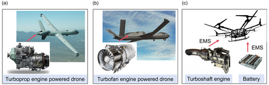
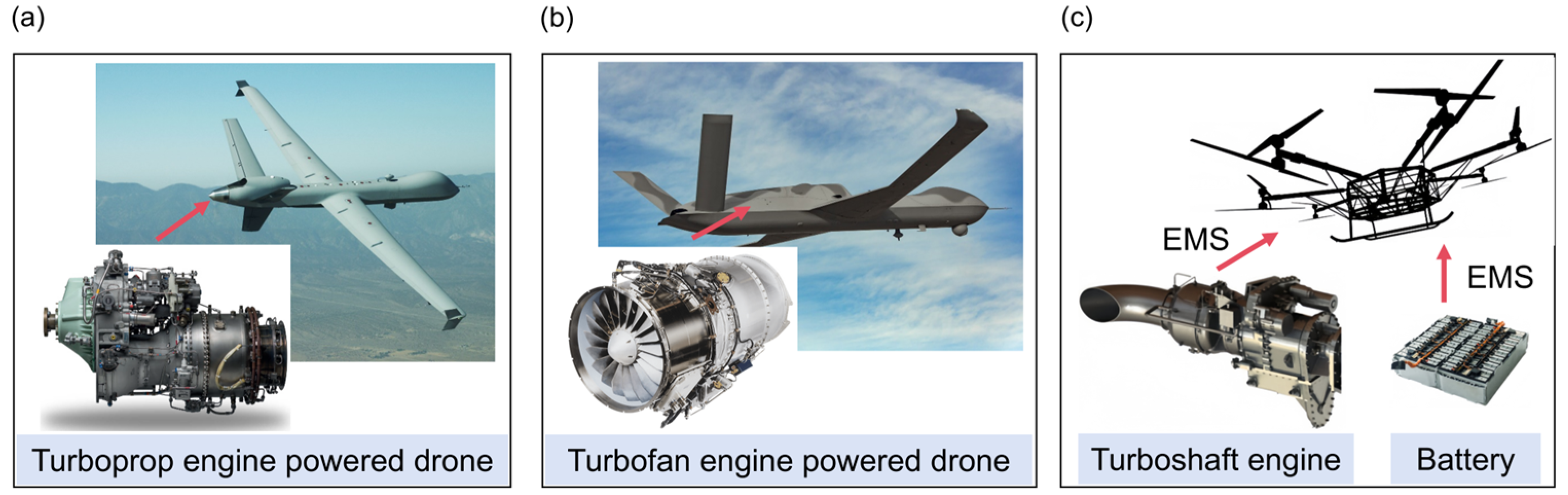
For long-endurance UAVs, especially those with significant weight operating at medium-to-high altitudes, conventional turbine engines still play a crucial role in the propulsion system [1,2], as shown in Figure 1. Turboprop engines occupy a great market share by virtue of their economic performance [3]. The widely used MQ-9 Reaper UAV, relying on its powerful TPE331-10 turboprop engine, can achieve 27 h endurance, while lithium-ion battery UAVs generally sustain flight of 2–10 h [4,5]. Turbofan engines can provide great thrust, which reduces the runway length requirement, lifts the accessible altitudes, and extends the endurance. Hybrid electric UAVs tend to equip turboshaft engines because of their high power-to-mass ratio [6]. Through an efficient energy management strategy (EMS), a hybrid drone that comprises a turboshaft engine generator pack and a battery pack can extend the flight range that a pure-electric one is limited to [7].

Figure 1. Turbine engine-powered long-endurance drones. (a) Turboprop engine; (b) turbofan engine; and (c) hybrid electric power system [8].

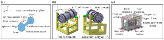
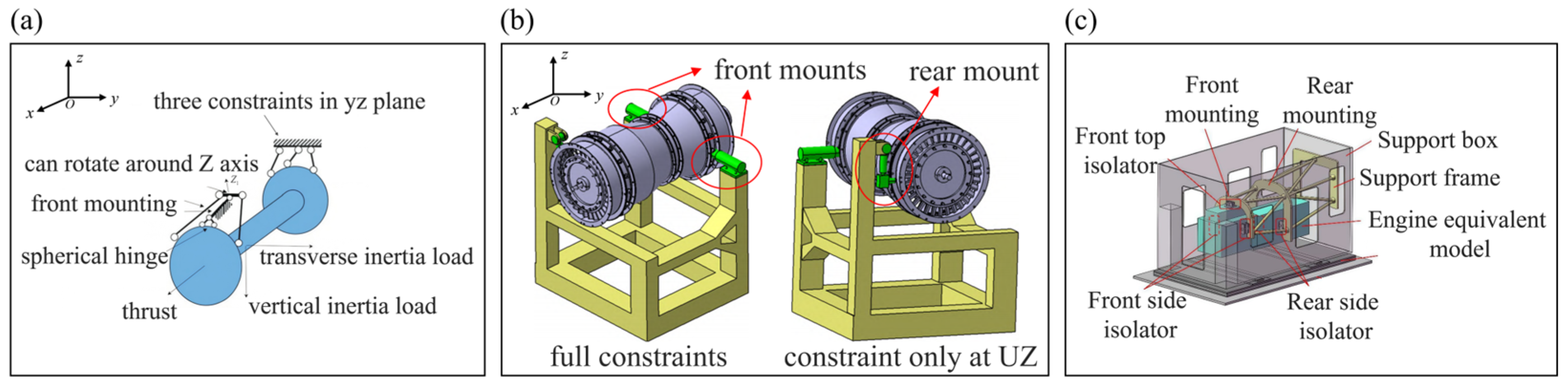
Monitoring rotor unbalance is an indispensable function of the UAV turbine engine health monitoring system [9]. Similar to the potential risks that quadrotor aircraft may face [10,11], foreign object damage (FOD), unexpected high-cycle fatigue cracks, erosion, and so forth can cause mass loss of turbine engine rotors, thereby inducing excessive unbalance-induced vibration [12,13,14]. Nevertheless, monitoring rotor unbalance in UAV turbine engines (and in some ducted engines) may be more challenging, because the rotor-stator coupling vibration effect has to be considered [15,16,17]. This effect is essentially absent in quadrotor aircraft [18,19,20]. Moreover, different engine mounting strategies result in different coupling vibration effects. Typical strategies applied in the long-endurance UAV platforms are shown in Figure 2. These mounting strategies can complicate the stator’s mechanical properties, for example, resulting in anisotropic supporting stiffness.

Figure 2. Typical engine mounting strategies applied in long-endurance UAV platforms. (a) Strategy1 [21]; (b) strategy2 [22]; and (c) strategy3 [23].

The diagnostic challenges introduced by the UAV installations mainly stem from two aspects. Firstly, achieving high-precision simulation modeling is more difficult, which particularly impacts the performance of model-based diagnostic methods. For one thing, it is hard to accurately characterize the mechanical properties of the installation constraints. For another, the anisotropic supporting stiffness results in additional critical speeds [24], making it difficult to ensure the consistency between the simulation model and the actual setup. Secondly, the response characteristics are more complex, posing challenges to data-driven diagnostic methods. Compared to the circular precession orbits observed under isotropic stiffness, it is harder to depict the features of elliptical precession orbits; moreover, the latter are influenced by more modal shapes than the former.

In the scope of rotor unbalance localization and identification, existing methods can be generally categorized into two groups: model-based methods and data-driven methods [25]. Model-based methods include the influence coefficient method (ICM), the modal balancing method (MBM), the equivalent load minimization method, etc. Among those, the ICM is one of the most classic techniques. Xia [26] investigated the unbalance identification of a single-disk system under sudden unbalance. MBM is another classic technique, designed especially for flexible rotors. The equivalent load minimization tackles unbalance diagnosis problems from the perspective of directly identifying the unbalance excitation itself, rather than specific amplitudes or phases. Liang [27] chose the augmented Kalman filter as the optimization algorithm to minimize the unbalance equivalent load and improved it with the convergence criterion.

Data-driven methods have flourished over the past two decades due to their robust mapping capabilities. Garoli [28] compared deterministic and stochastic approaches. Diverse machine learning tools have been investigated for rotor unbalance fault diagnosis, as well as for various other anomaly detection applications [29,30]. Among these, the convolutional neural network (CNN) is one of the most widely used architectures owing to its exceptional performance in image learning. Although direct application of raw time-domain signals is theoretically feasible, some studies prefer to incorporate a preprocessing step before inputting data into the CNN. For instance, Zhu [31] transformed vibration signals into symmetrized dot patterns.

In this work, the physics-informed neural network (PINN) acts as the guideline for solving unbalance localization and identification. To the best of the authors’ knowledge, little research has been conducted on designing an efficient PINN method for the multi-disk rotor-bearing-casing system with anisotropic supporting stiffness. By capturing the characteristics of actual engine mounts, this system is representative of engine installation status on the UAV platform [22,32]. In spite of recent advances, the PINN technique applied to fault diagnosis is still in its infancy [33,34,35,36].

Deng [37] categorized existing work into three classes: physics-informed input space, physics-embedded algorithm structure, and physics-constrained learning. The first class involves compensating for the lack of certain datasets or obtaining measurements from inaccessible locations. Freeman [38] combined the fault features from the high-fidelity numerical model with the environmental condition data. The second class features physical knowledge merged into the input layer, the hidden layer, or the process of the weight update. Liu [39] assessed the health condition by identifying the ordinary differential equations of the system under rotor unbalance excitation. The third class means that the loss function of a neural network contains analytical expressions from physical principles. Garpelli [40] investigated the performance of the proposed PGNN, whose highlight lies in the physical loss function.

According to the above taxonomy of PINN, the proposed PICNN in this paper belongs to the second class, namely the physics-embedded algorithm structure. Moreover, the physical knowledge here is in the form of FRF of the dynamic system and is embedded in the input layer of PICNN. Vibration response signals, along with the speed signal, first go into the PI layer and then go into different lightweight CNNs based on outputs from the PI layer. The core idea of the proposed PICNN is to spare the CNN from directly mapping the relations between unbalance parameters of multiple disks and measurements under various situations. It is the FRF of the dynamic model that takes responsibility for localizing the axial positions of dominant faulty disks. Afterwards, the lightweight CNN takes its turn to identify the unbalance amplitude and phase. In this paper, the terminology “dominant faulty disk” refers to the disk whose unbalance amplitude is the biggest among all the disks, and is more than ten times the amplitudes of others.

The novelty of the proposed PICNN method lies in three aspects. First, a physically interpretable FRF-based unbalance localization approach is demonstrated to be feasible even when the anisotropic supporting stiffness exists. The robustness against various sources of modeling errors (bearing stiffness, mounting stiffness, and damping ratio) is thoroughly investigated. Although the FRF is not new to the field, the capacity of FRF-based unbalance localization has not been thoroughly demonstrated before, especially the insensitivity to model precision in the multi-disk rotor-bearing-casing system. Second, with the aid of the PI layer, the identification precision can increase compared to pure data-driven counterparts. The elimination of negligible unbalance parameters has been demonstrated to promote more precise mapping, which has not yet been disclosed for a multi-disk rotor unbalance regression task. Third, the strength in computational efficiency is also observed.

The remaining part of this paper is organized as follows. Section 2 thoroughly presents the framework of the proposed method, from the general roadmap to detailed layer structures. Then, numerical cases (Section 3) and the experimental case (Section 4) are provided. The Discussion (Section 5) demonstrates the reliability of PICNN. Conclusions are summarized in Section 6.

2. The Framework of PICNN

2.1. The Roadmap of the Proposed Method

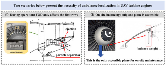
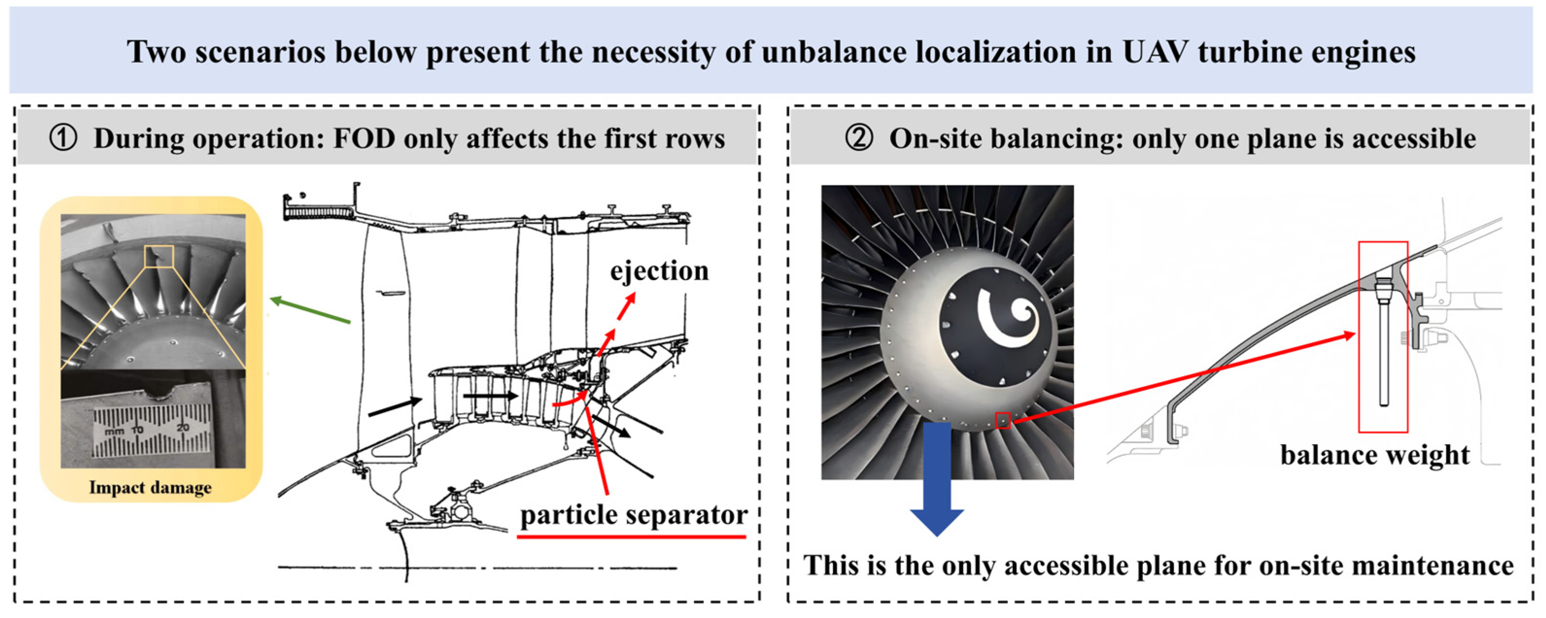
Taking the turbofan engine as an example, in engineering practice (Figure 3), it is meaningful to first determine the unbalance (or equivalent weight) positions, whether during the operation or during the on-site balancing scenario. For example, the foreign object damage (FOD) tends to affect the first rows of compressor blades [41], while the axially back part of blades may be safe and sound thanks to devices such as the particle separator located after the boosting stages. In that scenario, attention should be focused on the first rows. For another, during the on-site balancing, parameters of equivalent weights are the concern, including the mass, phases, and balancing planes. Considering that there is only one accessible plane for the on-site maintenance [42,43], it is crucial to first judge the axial positions of the equivalent weights. As long as the only accessible plane for the on-site maintenance belongs to the effective balancing planes, adding weights is effective; otherwise, more inaccessible balancing planes are entailed, and that means the engine has to be disassembled.

Figure 3. The engineering scenarios for the necessity of unbalance localization in UAV turbine engines.

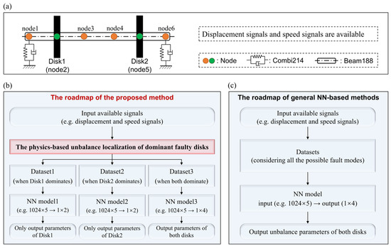
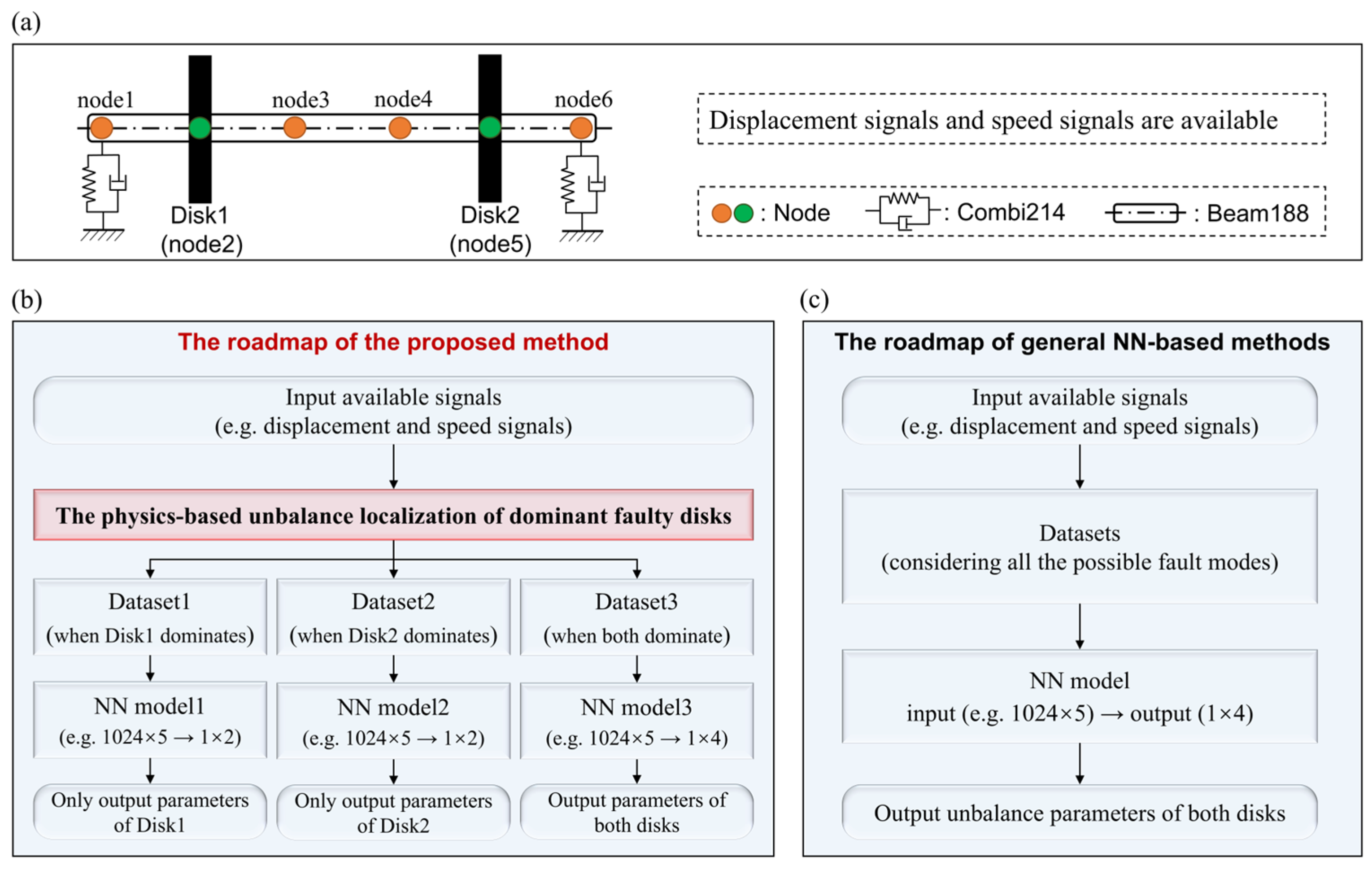
The roadmap of the proposed method is shown in Figure 4b. Taking the rotor-bearing system in Figure 4a as an example, the differences between the proposed method and the general NN-based methods can be summarized in three aspects below (roadmap A represents the proposed method, and roadmap B represents the general one in the literature). In addition, it is necessary to point out that the roadmap A differs from the ensemble learning method [44]. Only one of the NN models (1, 2, and 3) in the roadmap A is triggered, while all the sub-networks are triggered in the ensemble learning method.

Figure 4. The differences in roadmaps: (a) the schematic diagram of a typical rotor-bearing system; (b) the roadmap of the proposed method; and (c) the roadmap of general NN-based methods.

• Datasets. According to the outputs from the localization procedure, roadmap A divides the datasets and allocates them to different sub-networks trained for different tasks. Roadmap B gathers all the datasets under various fault modes to nurture an all-round neural network that can handle the unbalance identification of all possible components.
• Outputs. Roadmap A only focuses on the dominant parameters, while the outputs of roadmap B consist of the unbalance parameters of all disks.
• Precision and efficiency. Based on the same datasets and network structures, the precision achieved by roadmap A is higher, and that will be detailed in the following sections. Additionally, because the network models involved in the roadmap A and B are totally the same except for the output dimension, the hyperparameters involved in the roadmap A are consequently fewer, which means better training efficiency.

2.2. The Structure of the Unbalance Localization Layer

It is the frequency response function of the dynamic system that helps judge the dominant faulty disk. That distinguishes the PICNN method from purely data-driven methods and ensures the physical interpretability of the localization procedure. Unbalance identification is a typical inverse problem in dynamics. The excitation can be precisely obtained when we can get access to responses of all the degrees of freedom (DOFs) and establish the precise dynamic equations. Certainly, that prerequisite is nearly impossible in reality. However, what can be feasible is obtaining the excitation with some errors through measurements from a small number of DOFs. In terms of those reconstruction errors of excitation, they can be different according to different assumptions of the dominant excitation position.

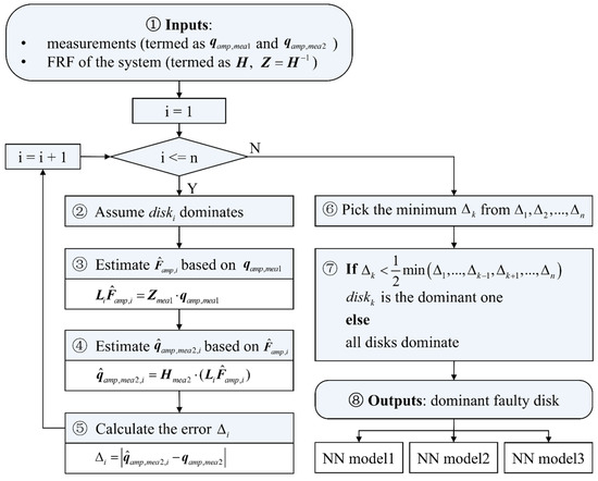
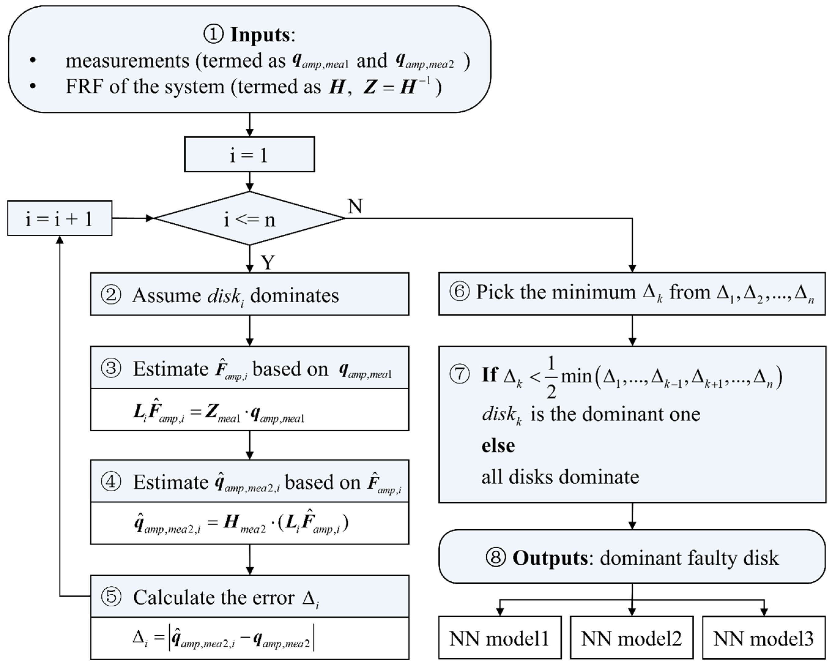
The reconstruction errors mentioned above inspire the core idea of the PI layer in this paper. The operational process is summarized in the flowchart as shown in Figure 5. Details are given below.

Figure 5. The structure of the localization layer (PI layer).

• Step ①: Inputs. What is needed includes the responses from two different positions (like node3-ux and node4-ux) and the FRF of the system.

Taking the twin-disk rotor-bearing system in Figure 4a as an example, the dynamic equations of the system under the healthy condition are presented in Equation (1):

$$\mathit{M}{\ddot{\mathit{q}}}_0+\left(\mathit{C}-\omega \mathit{G}\right){\dot{\mathit{q}}}_0+\mathit{K}{\mathit{q}}_0={\mathit{F}}_0$$

(1)

where $\mathit{M},\mathit{K},\mathit{C},\mathit{G}\in {ℝ}^{n_{dof}\times n_{dof}}$ are the mass matrix, stiffness matrix, damping matrix, and gyroscopic matrix, respectively. $n_{dof}$ is the number of DOFs of the dynamic system. $\omega$ is the rotating speed. ${\mathit{F}}_0\in {ℝ}^{n_{dof}\times 1}$ is the initial unbalance force and is inevitable in reality. ${\mathit{q}}_0\in {ℝ}^{n_{dof}\times 1}$ is the corresponding displacement.

When the system encounters extra unbalance excitation, the equation is given in Equation (2):

$$\mathit{M}{\ddot{\mathit{q}}}_f+\left(\mathit{C}-\omega \mathit{G}\right){\dot{\mathit{q}}}_f+\mathit{K}{\mathit{q}}_f={\mathit{F}}_0+{\displaystyle \sum _{e=1}^m{L}_e\cdot F_e}$$

(2)

where ${\mathit{F}}_e\in {ℝ}^{n_{excite}\times 1}$ is the extra unbalance force, ${\mathit{L}}_e\in {ℝ}^{n_{dof}\times n_{excite}}$ specifies the excitation position, and m is the number of nodes where unbalance may exist. Subtract Equation (1) from Equation (2), and the resulting Equation (3) is given below:

$$\mathit{M}\ddot{\mathit{q}}+\left(\mathit{C}-\omega \mathit{G}\right)\dot{\mathit{q}}+\mathit{Kq}={\displaystyle \sum _{e=1}^m{L}_e\cdot F_e}$$

(3)

where the residual response $\mathit{q}$ can be obtained as $\mathit{q}={\mathit{q}}_f-{\mathit{q}}_0$.

Then, expand $\mathit{q}$ and ${\mathit{F}}_e$, following the Fourier law:

$$\mathit{q}={\displaystyle \sum _{k=0}^{\infty }({\mathit{q}}_{amp}^{[k]}\cdot e^{jkwt})}, {\mathit{F}}_e={\displaystyle \sum _{k=0}^{\infty }({\mathit{F}}_{amp,e}^{[k]}\cdot e^{jkwt})}$$

(4)

where k is the harmonic order.

• Step ②: Make assumptions. The parameter n (in the previous decision box) is equal to the number of disks.

Considering that only the unbalance excitation is involved, Equation (4) is transformed into Equation (5):

$$\mathit{q}={\mathit{q}}_{amp}^{[1]}\cdot e^{jwt}={\mathit{q}}_{amp}\cdot e^{jwt}, {\mathit{F}}_e={\mathit{F}}_{amp,e}^{[1]}\cdot e^{jwt}={\mathit{F}}_{amp,e}\cdot e^{jwt}$$

(5)

where ${\mathit{q}}_{amp}^{[1]}$ and ${\mathit{F}}_{amp,e}^{[1]}$ are represented as ${\mathit{q}}_{amp}$ and ${\mathit{F}}_{amp,e}$ respectively, which is to simplify the representation.

• Steps ③–⑤: Calculate a criterion. An estimation error is finally obtained to represent the precision of the assumption.

Substitute Equation (5) into Equation (3), and the resulting equation is presented in Equation (6):

$$\mathit{Z}\cdot {\mathit{q}}_{amp}={\displaystyle \sum _{e=1}^m({\mathit{L}}_e\cdot {\mathit{F}}_{amp,e})}$$

(6)

where $\mathit{Z}=(-{\omega }^2\mathit{M}+j\omega (\mathit{C}-\omega \mathit{G})+\mathit{K})$.

For the twin-disk rotor-bearing system, the parameter m in Equation (6) is equal to 2. Now, let us first assume the dominant faulty disk is Disk1. For the situation that disk2 dominates, the deduction is similar. Assuming that Disk1 dominates, which means only the excitation on Disk1 is considered, Equation (6) is transformed into Equation (7):

$${\mathit{L}}_1{\hat{\mathit{F}}}_{amp,1}={\mathit{Z}}_{mea1}\cdot {\mathit{q}}_{amp,mea1}$$

(7)

where mea1 represents the response from one of the DOFs (e.g., node3-ux). Through ${\mathit{Z}}_{mea1}$ and ${\mathit{q}}_{amp,mea1}$, the complex amplitude of the excitation on Disk1, namely ${\hat{\mathit{F}}}_{amp,1}$, can be estimated.

Substitute the ${\hat{\mathit{F}}}_{amp,1}$ obtained from Equation (7) into Equation (8):

$${\hat{\mathit{q}}}_{amp,mea2,1}={\mathit{H}}_{mea2}\cdot ({\mathit{L}}_1{\hat{\mathit{F}}}_{amp,1})$$

(8)

where $\mathit{H}$ is the FRF of the dynamic system, $\mathit{H}=inv(\mathit{Z})$, and mea2 is the response from another DOF (e.g., node4-ux).

Compare the estimation ${\hat{\mathit{q}}}_{amp,mea2,1}$ and the real value ${\mathit{q}}_{amp,mea2}$ at mea2, the error can be obtained by Equation (9)

$${\Delta }_1=\left|{\hat{\mathit{q}}}_{amp,mea2,1}-{\mathit{q}}_{amp,mea2}\right|$$

(9)

where ${\Delta }_1$ physically represents the error when Disk1 is assumed to be the dominant one.

• Steps ⑥–⑧: Choose the best assumption and output the dominant faulty disk. The assumption whose error is smaller than half of the minimum of the others is determined as the best one.

Similarly, ${\Delta }_2$ can be obtained. If ${\Delta }_1\ll {\Delta }_2$, that means Disk1 exerts much more influence on the measured responses; consequently, the PI layer outputs Disk1 as the dominant disk, and vice versa. Here, the exact metric of outputting Disk1 as the dominant disk is ${\Delta }_1<{\Delta }_2/2$.

It is noteworthy that the procedure above totally depends on the dynamic model of the system (more specifically, the FRF) and therefore belongs to model-based techniques. That distinguishes itself from some data-driven localization methods, such as BP-ANN [45] and 1D-CNN [46].

2.3. The Structure of the Unbalance Identification Layer

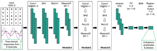
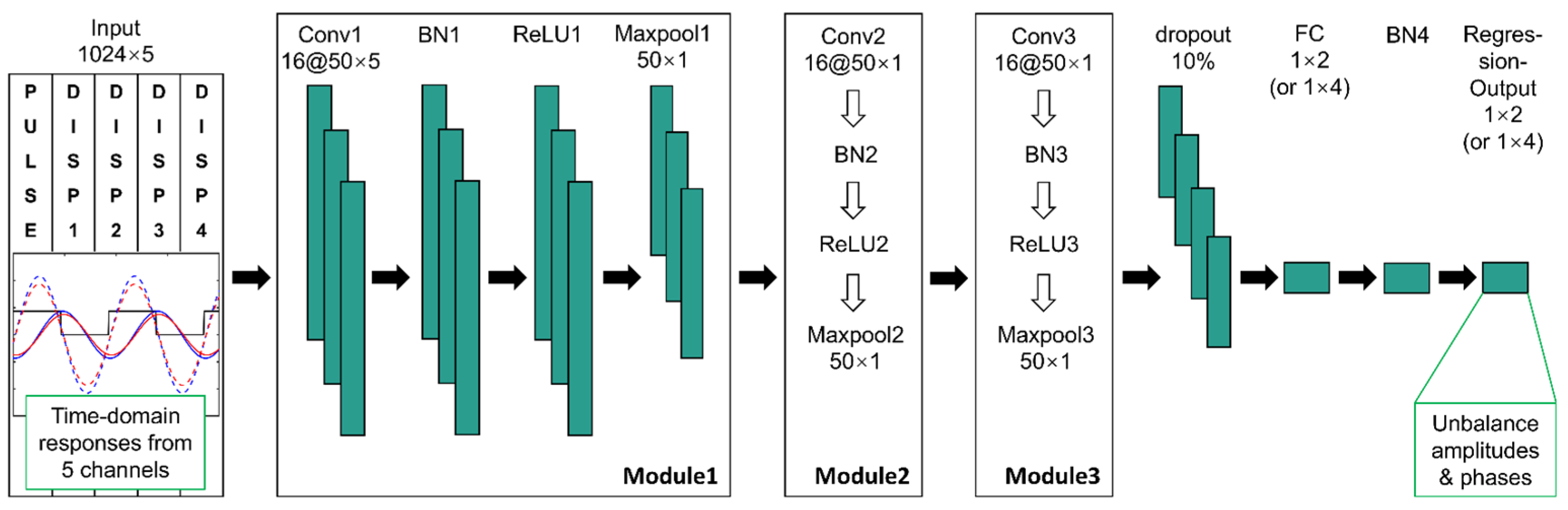
Following the roadmap in Figure 4b, the NN model is illustrated in Figure 6. Here, according to the output from the PI layer, a lightweight CNN is established to further identify the unbalance parameters.

Figure 6. The lightweight CNN employed in the PICNN method.

The inputs include the pulse signal (reflecting the rotating speed) and vibration responses from four different DOFs, all of which are in the time domain. The dimension of the input sample is 1024 × 5, where 1024 represents the number of time-domain sampling data, and 5 represents the number of data-collection channels. The outputs are the unbalance amplitudes and phases of the dominant faulty disks. The dimension of outputs is 1 × 2 or 1 × 4, which depends on the number of dominant disks. The regression processes of unbalance amplitudes and phases operate simultaneously.

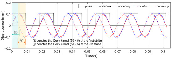
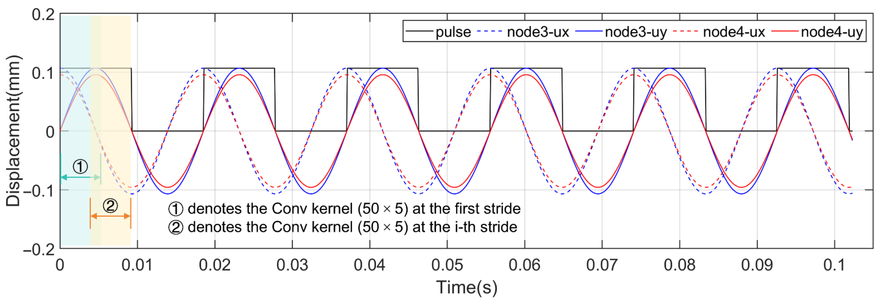
The lightweight CNN only consists of three convolution layers. The structures of modules 1–3 in Figure 6 are similar. In the beginning, the number of channels in the input sample is 1. The convolution layer 1, whose kernel size is 50 × 5, firstly processes the input sample and produces 16 channels. Figure 7 provides insight into the design rationale of the kernel size. The 50-dimensional length is designed to encompass the global features of sinusoidal waveforms, extracting both amplitude and phase information concurrently. The five-dimensional length is set to ensure the parallel processing of the five-channel input. An ablation study on kernel size will be presented afterwards to demonstrate the insensitivity to such variations. The stride is 1; no padding is applied. Here, the response phase means the value that the response peak is behind the pulse’s rising edge.

Figure 7. The illustration about the function of the first convolution kernel (in the size of 50 × 5).

The above settings (except the kernel size) of Conv1 are the same in Conv2 and Conv3. The input size of the batch-normalization (BN) layer (1–3) is 16. The activation function is ReLU. The max pooling layer (1–3) works after the activation, with its kernel size of 50 × 1 and a stride of 1. The dropout layer with a probability of 10% is designed to avoid overfitting. Following the dropout layer, the fully connected (FC) layer linearly transforms the incoming data (resized to one-dimensional tensors) to fit the output sample, whose dimension is 1 × 2 for NN models 1 and 2 (in Figure 4b), and is 1 × 4 for NN model 3 (in Figure 4b). In the end, the batch-normalization layer 4 works, and its size also depends on the triggered sub-networks.

The training hyperparameters are listed in Table 1. The training optimizer is Adam, with a learning rate of 0.01. The loss function is based on the mean absolute error (MAE). The batch size during training is 40. The training epoch is 2000. The early stopping strategy is given a tolerant patience mechanism to prevent both overfitting and underfitting. When the validation loss does not decrease, a tolerant patience mechanism is applied, which allows the validation loss to search for its lower value within the upper bound of 2000 epochs. Under the prerequisite that the training loss declines, the best epoch is the one where the validation loss declines to the minimum during the given epochs. The random seed is fixed with an index of 300, ensuring replication. The system hardware and software specifications are shown in Table 2. The above settings are applied consistently across the following numerical and experimental cases.

Table 1. The training hyperparameters.

Item	Setting
Optimizer	Adam
LR schedule	Keep 0.01
Epochs	2000
Batch size	40
Early stopping	Yes
Loss function	Mean absolute error
The criterion for selecting the best epoch	The one that achieves the minimum validating loss

Table 2. System hardware and software specifications.

Operating System	Processor	RAM	Execution Environment	GPU	Execution Mode
Microsoft Windows 10 Enterprise (Build 19045)	Intel Core i7-10700 (8 cores, 16 threads, 2.90 GHz)	64 GB (63.8 GB usable)	PyCharm (Community Edition 2023.3.4) (Python 3.11.8, with PyTorch 2.2.1.)	NVIDIA GeForce GTX 1660 SUPER	GPU

The structure in Figure 6 only consists of three convolution layers, which is lightweight compared to other classical CNN models such as ResNet34 [47]. In the following pages, the performance of the proposed PICNN will be compared with pure data-driven methods, including the pure-CNN method and the pure ResNet34 method.

2.4. The Arrangement of the Datasets

The previous section focuses on the NN structure and briefly introduces the input and output samples. In this section, more details about the datasets are presented. The arrangement strategy is applied consistently across the following numerical and experimental cases. Taking the rotor-bearing system in Figure 4a as an example, details of the inputs are given below.

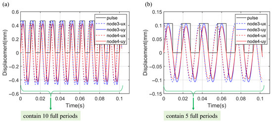
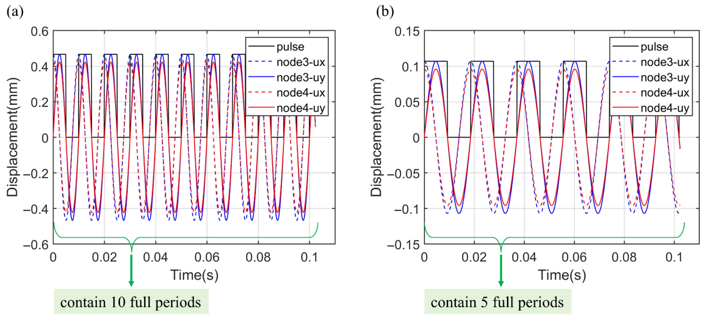
Firstly, the number 1024 is determined to contain enough full periods. As illustrated in Figure 8, when the sampling frequency is set to 10 kHz, the number of full periods varies under different rotating speeds. Here, the input requires at least five full periods to include sufficient information for CNN feature extraction. The chosen number, 1024, can meet that requirement within the concerned speed range (over 50 Hz). In addition, the number 1024 can be represented as 32 × 32, whose representation conforms to the input format of some benchmark CNN models like ResNet34; therefore, choosing the number 1024 is also convenient to conduct a comparison among different methods. In terms of other higher sampling frequencies, e.g., 50 kHz, down-sampling can be applied to meet the five-full-period requirement.

Figure 8. The illustration of the requirement of the time length: (a) under the rotating speed of 100 Hz and (b) under the rotating speed of 54 Hz.

Secondly, the amplitude of the square pulse is set to be the same as that of the displacement response (e.g., node3-ux). That processing aims to avoid extremely big (or small) values spoiling the feature extraction. For the numerical datasets, the rising edge of the pulse signal is fixed on the origin of the time-axis, and therefore can simulate the response-phase differences under different unbalance configurations. For the experimental datasets, pulse signals (from the photoelectric transducer) and response signals (from eddy current sensors) are collected simultaneously, without the need for manual alignment. Thirdly, the min-max normalization is applied to the input samples. All of the training, validating, and testing input samples are normalized according to the minimum and maximum of the training datasets.

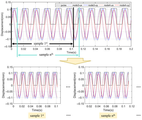
The input samples consist of multiple segments, each comprising 1024 sampling points extracted from the time-domain responses. Considering that the CNN model maps relations from the perspective of image recognition, it is meaningful to accommodate different segments under the same unbalance configuration (Figure 9). Those segments appear to be different in the view of the images. Actually, they physically belong to the same unbalance configuration and are expected to output the same unbalance parameters. The number of segments under the same unbalance mode will be presented in the following cases. The input response signals from experiments are filtered through FFT, and only the fundamental rotating frequency is retained.

Figure 9. The illustration of dividing the time-domain results under the same unbalance mode.

The output normalization is similar to the input normalization, namely the min–max approach. The unbalance amplitudes are scaled to the range [1 × 10⁻³, 1] according to their minimum and maximum in the training datasets; so are the unbalance phases. The value 1 × 10⁻³ is chosen as the normalized minimum to avoid potential risks such as the denominator being zero during the calculation of relative errors.

3. Numerical Cases

3.1. A Twin-Disk Rotor-Bearing System

The illustration and physical parameters of the twin-disk rotor-bearing system are presented in Figure 4a and Table 3, respectively. The rotating speed is 100 Hz. Adhering to the principle of the PICNN, the simulated pulse signal and the displacement responses from node3-ux, node3-uy, node4-ux, and node4-uy are chosen as the inputs. The datasets for training, validating, and testing are listed in Table A1 (see Appendix A), where the unbalance amplitude ranges from 1.0 × 10⁻⁴ to 9.487 × 10⁻⁴, and the phase ranges from −0.9 × $\pi$ to 0.998 × $\pi$. It is noteworthy to point out that the training, validating, and testing datasets do not overlap. For example, the same sample does not exist in both the training and the testing, ensuring the effectiveness of the results.

Table 3. The physical parameters of the twin-disk rotor-bearing system.

Shaft	Disk	Bearing
Density: 7.8 × 10−9 t/mm3	Disk1-mass: 1 × 10−2 t	Stiffness: 2.5 × 106 N/mm
Elastic modulus: 2.1 × 105 MPa	Disk2-mass: 4 × 10−3 t	Damping: 1 × 103 Ns/mm
Poisson’s ratio: 0.3	Disk1 polar moment of inertia: 100 t∙mm2
Length: 500 mm	Disk2 polar moment of inertia: 70 t∙mm2
Diameter: 36 mm	Disk1 diametric moment of inertia: 50 t∙mm2
	Disk2 diametric moment of inertia: 35 t∙mm2

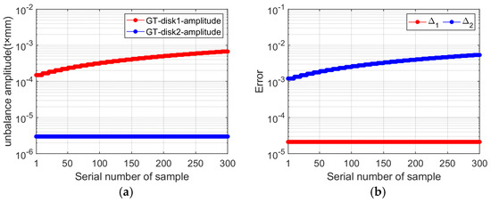
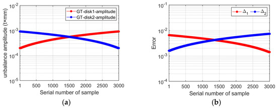
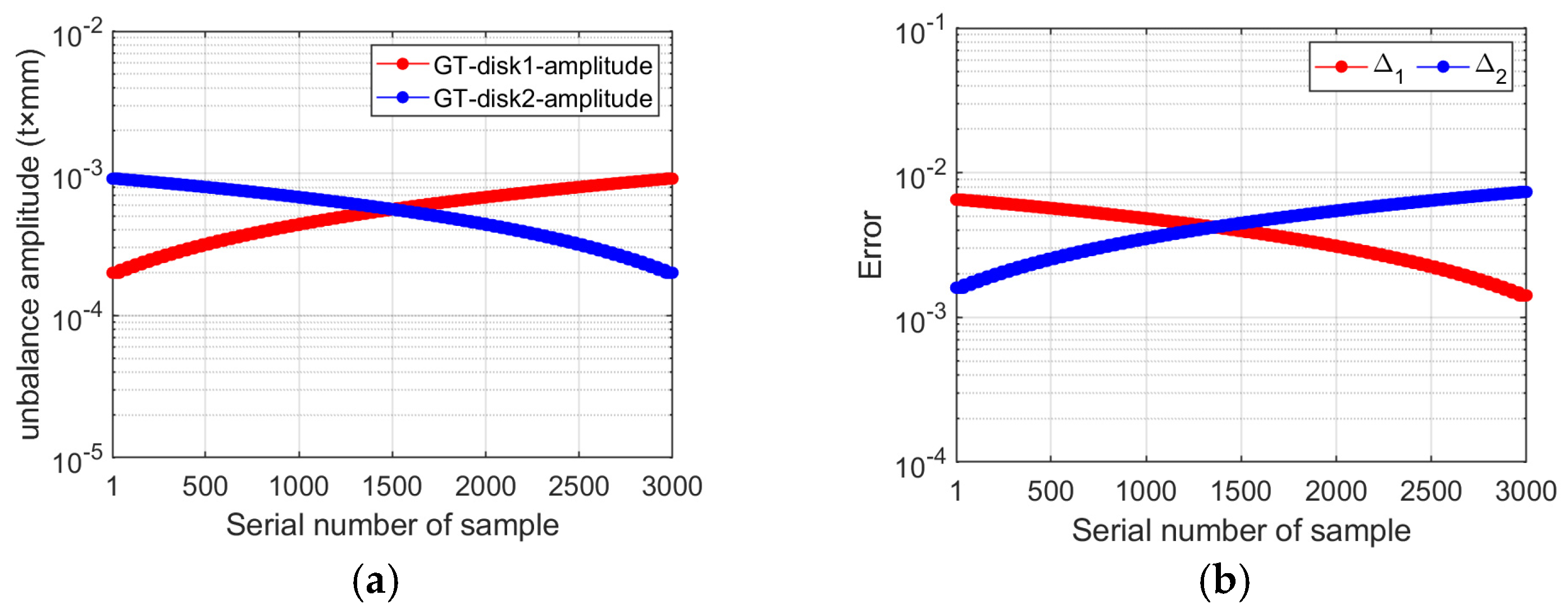
Firstly, the input signals go into the PI layer, and that layer outputs the judgment of the dominant faulty disk, as shown in Figure 10. It can be seen from Figure 10 that, when the ground truth (GT) of disk1-amplitude is greater than that of disk2-amplitude, the error of disk1 (denoted as ${\Delta }_1$) is remarkably smaller than ${\Delta }_2$. This represents that disk1 exerts much more influence on the measured responses than disk2. According to the criterion shown in Figure 5, the dominant faulty disk is localized to disk1.

Figure 10. The outputs of the PI layer for testing samples in dataset 1: (a) the ground truth and (b) the error output from the PI layer.

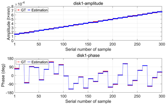
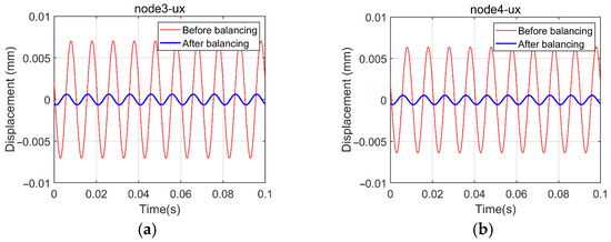
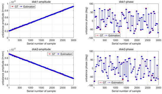
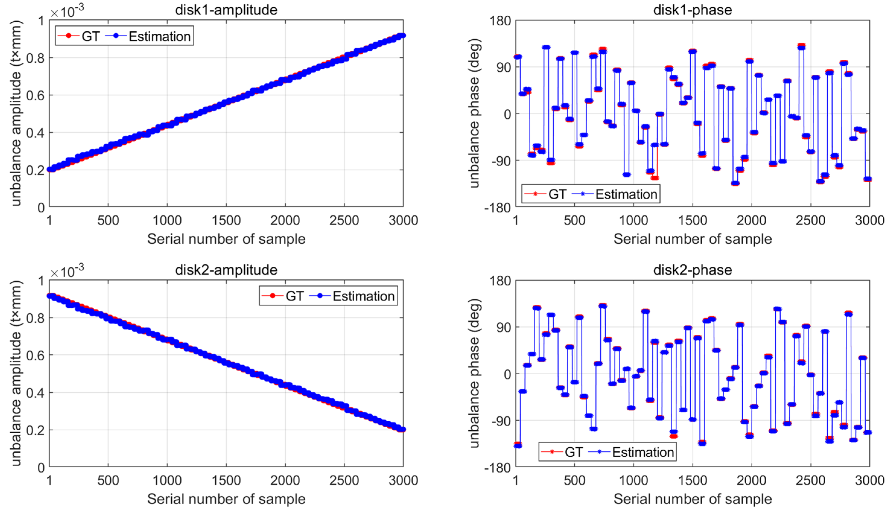
Afterwards, the NN model 1 trained by dataset 1 is triggered to predict the unbalance amplitude and phase of disk1, results presented in Figure 11. The relative error of disk1-amplitude is 0.798%, and that of disk1-phase is 5.15%. In this numerical case, the unbalance phase identification results all fall into the range of −180 degrees to 180 degrees. In addition, the scenario where the phase GT is 0 degrees is not designed; therefore, the calculation method for the relative error of the phase identification results is identical to that of the amplitude. Furthermore, the balancing results based on the estimated values from PICNN are given in Figure 12, where the first testing sample is presented as an instance. The amplitude reductions are 90.9% and 91.2% for node3-ux and node4-ux, respectively. In terms of dataset 2, the performance of PICNN is close to what we achieved in dataset 1. In dataset 2, the relative errors of the identification results are 0.973% for the disk2-amplitude and 3.43% for the disk2-phase.

Figure 11. The identification results from the PICNN when disk1 dominates.

Figure 12. The balancing results obtained by only considering the dominant faulty disk: (a) the displacement of node3 in the x-direction and (b) the displacement of node4 in the x-direction.

In the case that both disks dominate, the results from the PI layer are given in Figure 13. As can be seen from Figure 13, the differences in errors are less significant than those in Figure 10, particularly for the samples from 1000th to 2000th. This is because the ground truths of disk1 and disk2 are comparable in dataset 3. For these samples, according to the criterion shown in Figure 5, the PI layer then triggers the following NN model 3 to carry on the identification. The reliability of the PI layer will be further discussed in the following sections.

Figure 13. The outputs of the PI layer for testing samples in dataset 3: (a) the ground truth and (b) the error output from the PI layer.

When both disks dominate, the identification results from the PICNN are shown in Figure 14. The relative errors for disk1-amplitude, disk1-phase, disk2-amplitude, disk2-phase are 1.03%, 6.41%, 0.955%, 4.03%, respectively.

Figure 14. The identification results from the PICNN when both disks dominate.

Turning now to the results without the PI layer. To demonstrate the advantages of the proposed PICNN, pure-data-driven methods (pure-CNN and pure-ResNet34) are employed as comparisons. Lack of acquaintance with the dominant faulty disk, the pure-data-driven methods directly map the relations between input signals and unbalance parameters of all disks. The datasets assemble all three in Table A1. The structure of the pure-CNN in this paper is the same as what is shown in Figure 6, ensuring that the difference between PICNN and pure-CNN is only the PI layer. Results are presented in Figure 15 and Figure 16.

Figure 15. The identification results from the pure-CNN when only disk1 dominates.

Figure 16. The identification results from the pure-ResNet34 when only disk1 dominates.

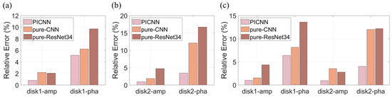
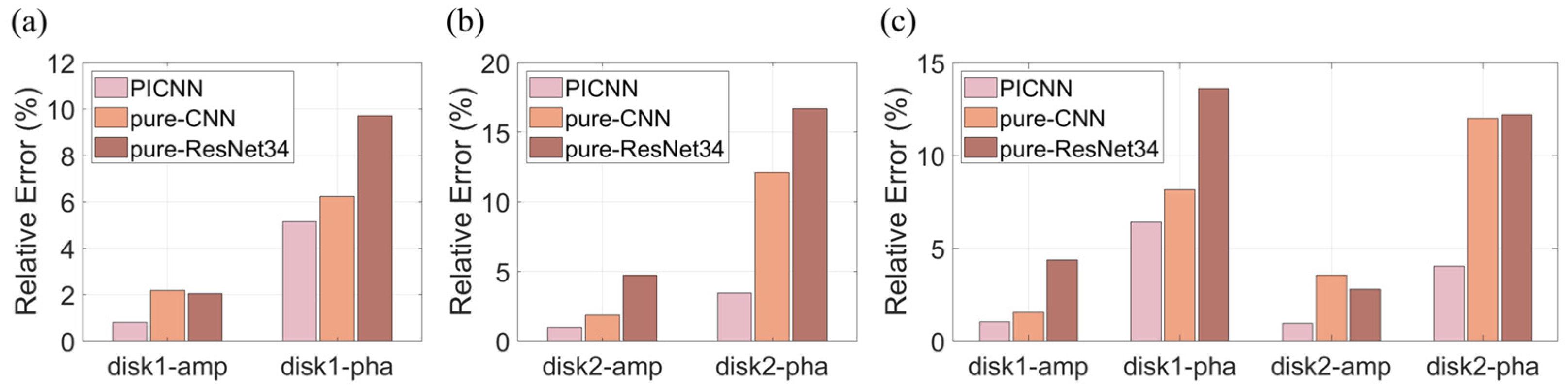
Figure 15 presents the estimated parameters based on the pure-CNN when disk1 dominates. The relative error of disk1-amplitude is 2.19%, and that of disk1-phase is 6.22%. Both are bigger than what is obtained in the PICNN (0.798% for the disk1-amplitude and 5.15% for the disk1-phase). In terms of the results for disk2, the relative errors are over 100%. Through the comparison between Figure 11 and Figure 15, it can be found that, when only disk1 dominates, the weakness of the pure-CNN is sparing its mapping ability for something unimportant. Consequently, it achieves lower precision on disk1 (main focus) and fails to identify the parameters of disk2; that is to say, under the same datasets and network structures, giving up the negligible components is conducive to improving the identification precision on what really counts. A similar phenomenon is presented in Figure 16, where the relative errors are 2.05% and 9.70% for disk1-amplitude and disk1-phase, respectively. Comparisons for other fault modes are provided in Figure 17, demonstrating the strengths of the proposed PICNN method.

Figure 17. The comparison among different methods: (a) when disk1 dominates, (b) when disk2 dominates, and (c) when both dominate.

The comparison of computational cost among different methods is shown in Table 4. Based on the same samples, the total time cost of PICNN is lower than that of other methods. Moreover, a great time saving (1.39 h vs. 18.7 h) for fault mode 1 (or 2) is noteworthy.

Table 4. Summary of the computational cost of different methods.

Method	Fault Mode	Total Samples	Number of Trainable Parameters	Time Cost
PICNN	mode 1	2400	5.31 × 104	1.39 h
	mode 2	2400	5.31 × 104	1.39 h
	mode 3	24,000	7.65 × 104	15.6 h
pure-CNN	cannot distinguish	28,800	7.65 × 104	18.7 h
pure-ResNet34	cannot distinguish	28,800	4.02 × 106	19.4 h

3.2. A Rotor-Bearing-Casing System

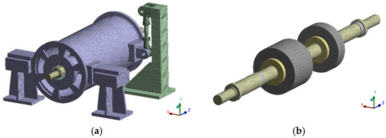
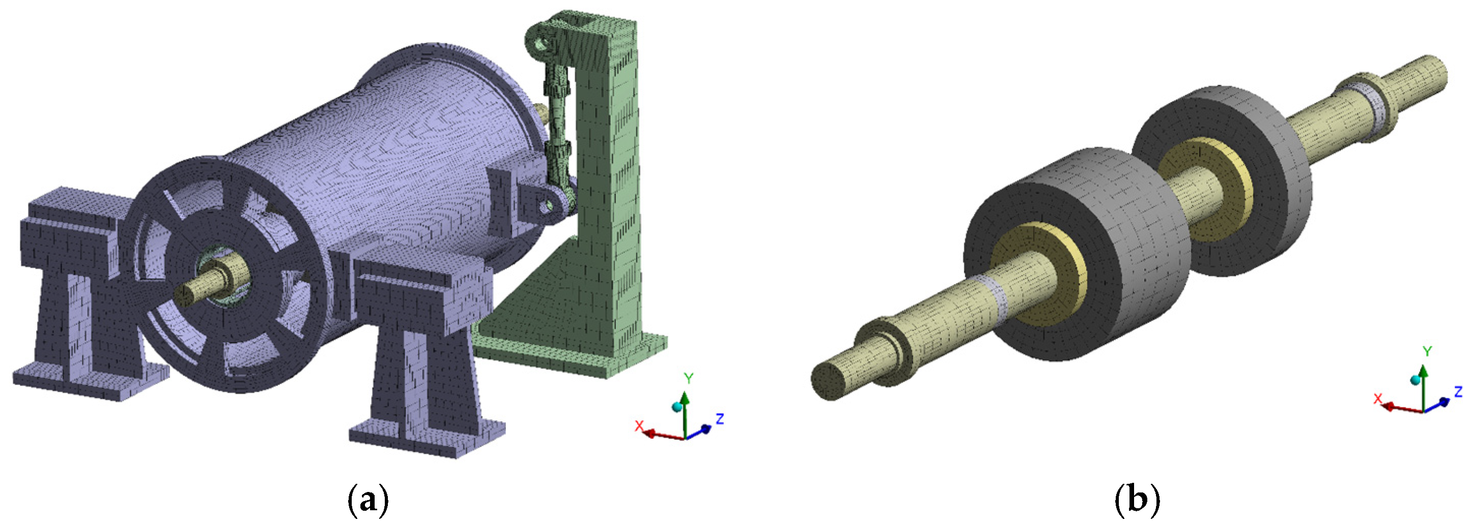
Next, we consider a more complex system, namely a rotor-bearing-casing system, as shown in Figure 18. This finite element model corresponds to the experimental setup in Section 4.1. The twin-disk rotor is supported by two bearings, while the flexible casing is supported by three mounts, one of which is achieved by a hinge joint. The Craig–Bampton component mode synthesis (CB-CMS) method is employed for model reduction with the first twenty modes retained. For simplification, the thicker disk in Figure 18b is termed the big disk, while the other is termed the small disk.

Figure 18. The finite element model of a rotor-bearing-casing system. (a) is the whole model; (b) is the rotor component.

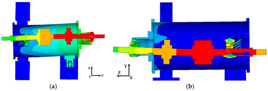
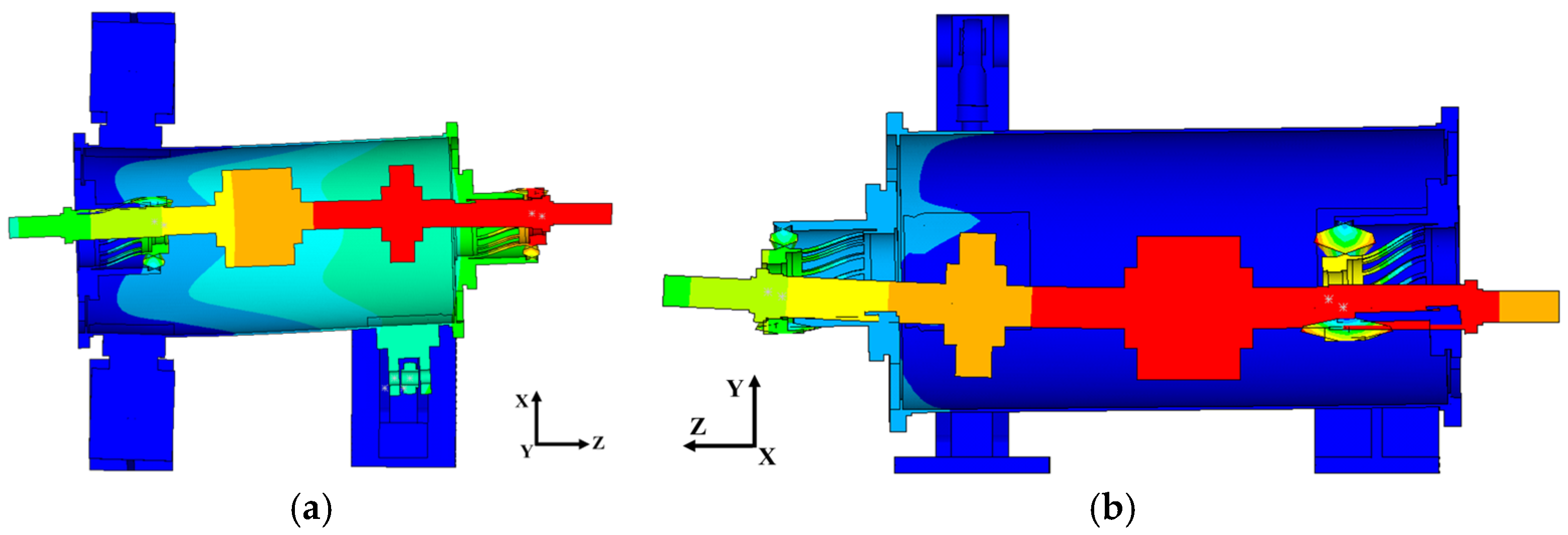
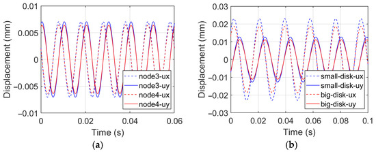
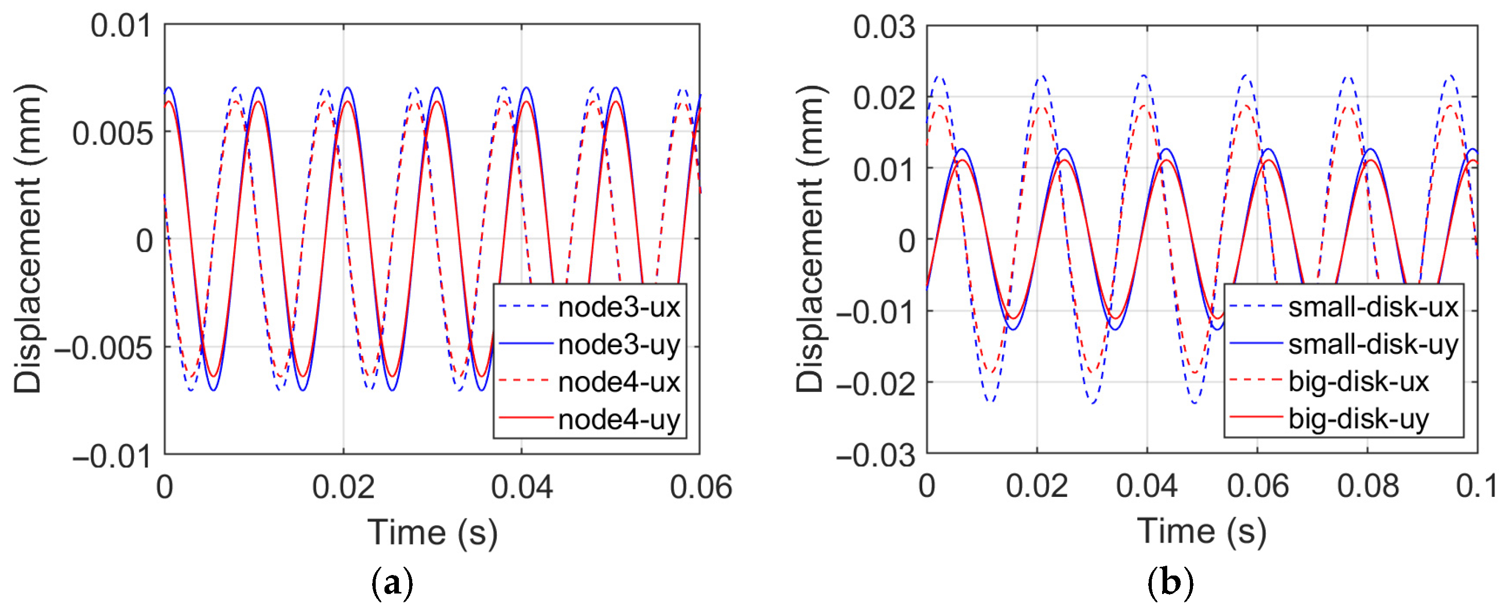
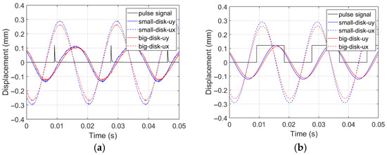
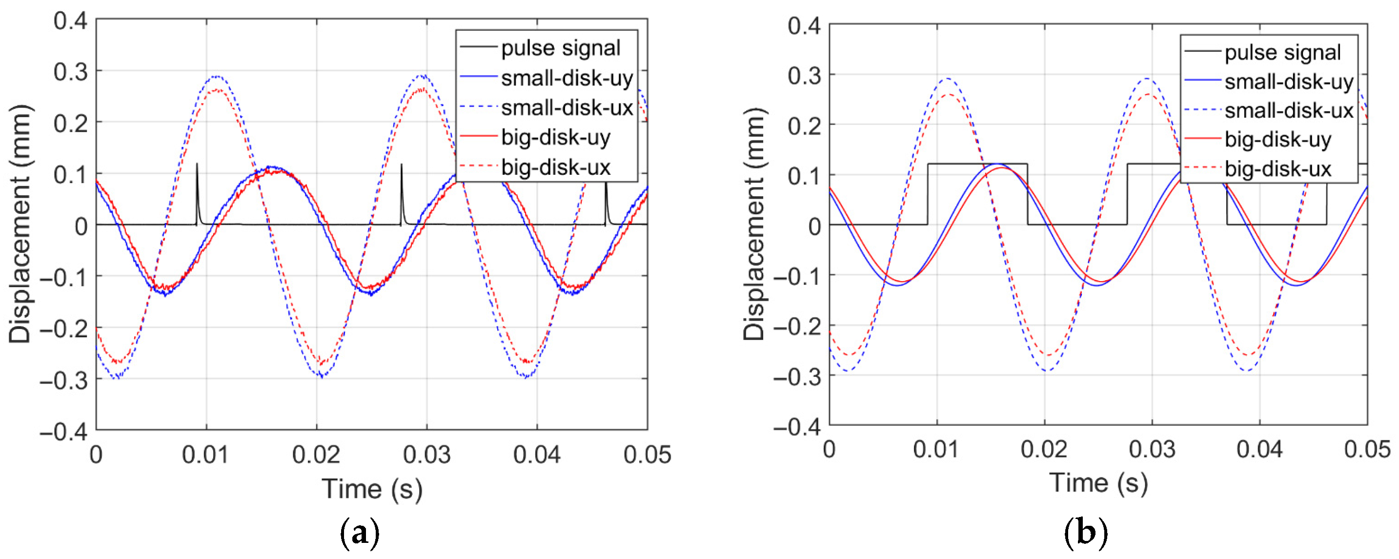
Before elaborating on the prediction performance, this section begins with the difficulty challenging the diagnostic method, namely, the anisotropic supporting stiffness, which was not involved in the previous section. Figure 19 presents the first backward and forward whirl modes of the system. Because of the anisotropic supporting stiffness, the modal frequencies of those modes differ greatly. Moreover, the differences in the horizontal (X-axis) and vertical (Y-axis) responses caused by the anisotropic supporting stiffness are given in Figure 20, which introduces additional feature-extraction pressure on the CNN model. In Figure 20b (and also the remaining parts of this paper), “small-disk-ux” means the horizontal displacement response of the small disk, while “small-disk-uy” means the vertical response.

Figure 19. The first two modes of the rotor-bearing-casing system: (a) the first backward whirl (68.2 Hz) and (b) the first forward whirl (75.2 Hz).

Figure 20. The differences in the displacement responses: (a) from the previous system without casing and (b) from the rotor-bearing-casing system in this section.

The input responses here include the speed pulse signal and displacements (both horizontal and vertical) of disks. The rotating frequency is 54 Hz. The dataset configuration is the same as Table A1, where the settings related to disk1 are applied to the small disk and those related to disk2 are applied to the big disk. The outputs of the PI layer are similar to previous results, succeeding in localizing the dominant disk.

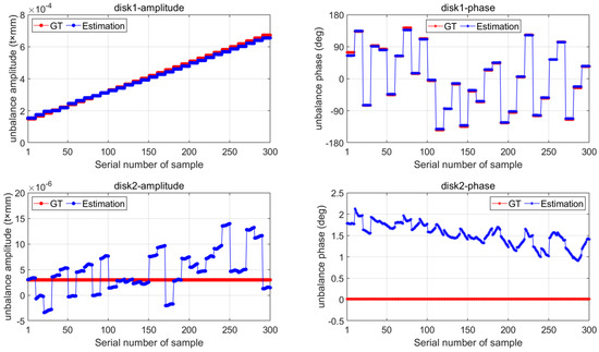
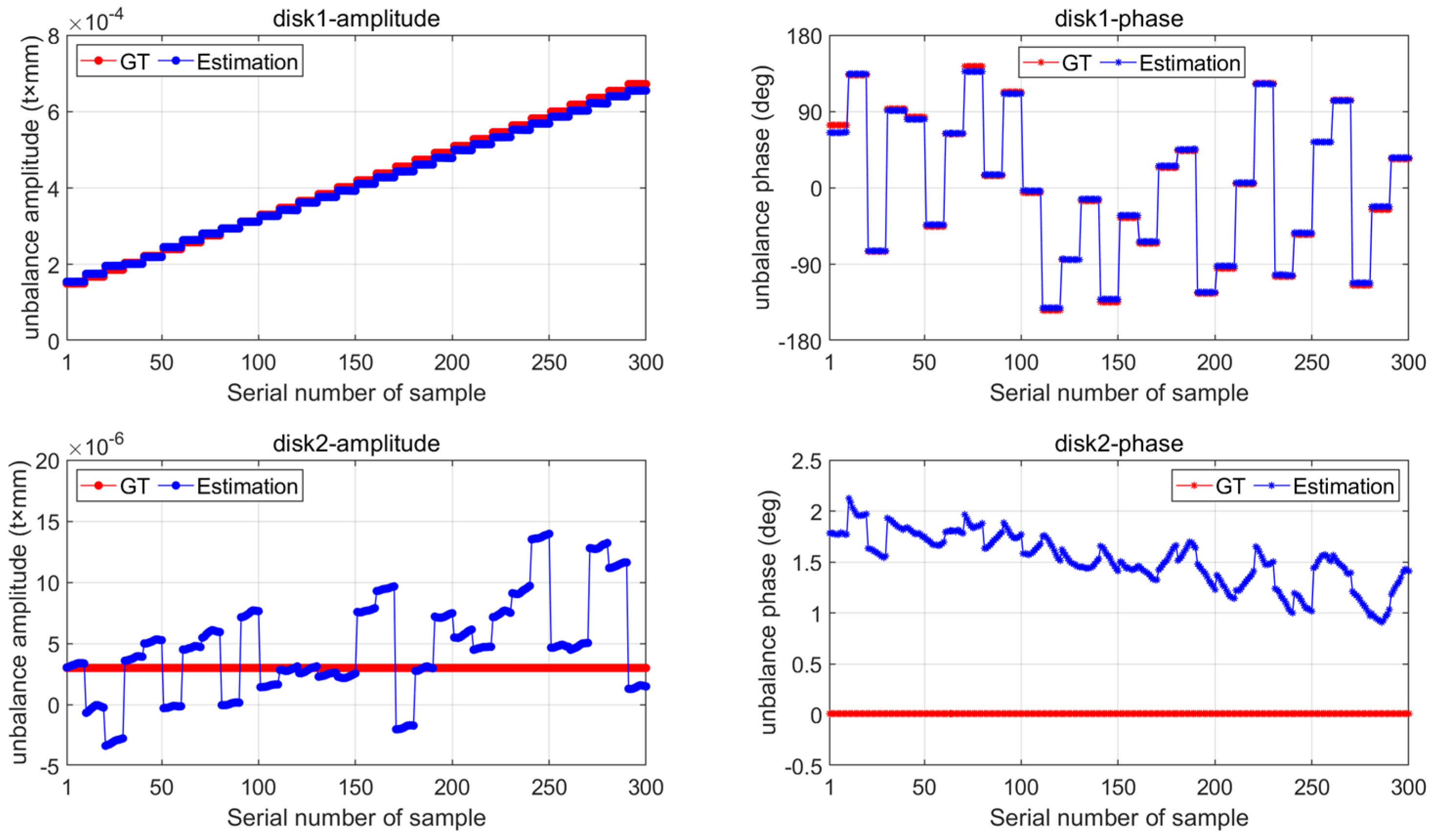
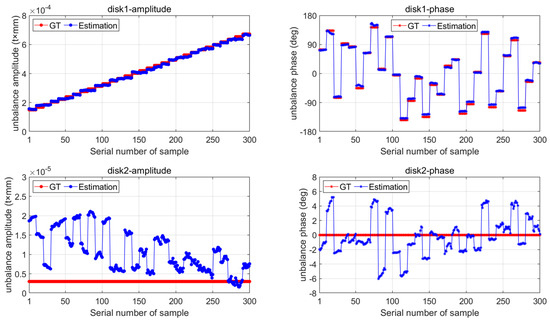
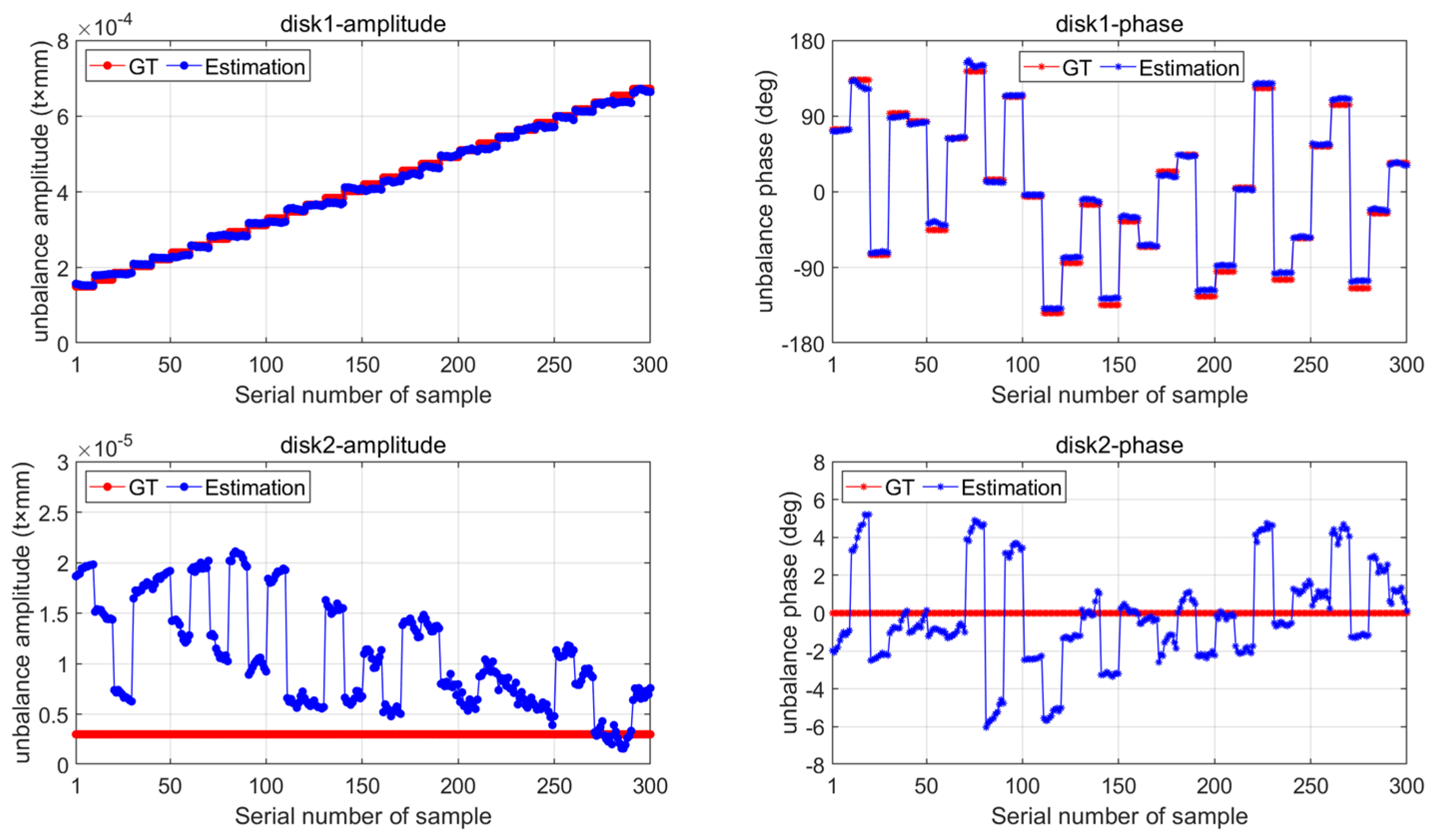
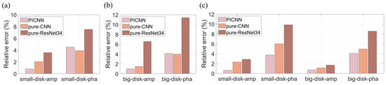
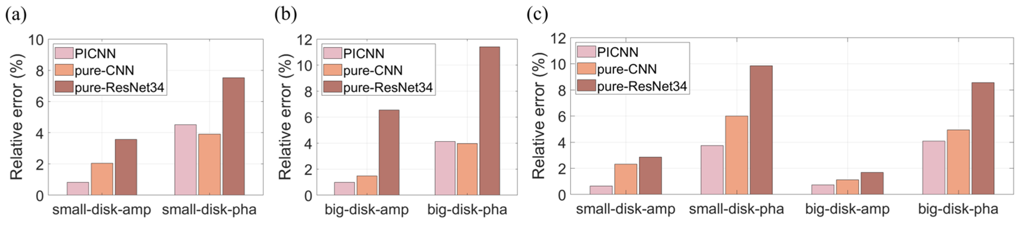
When the small disk dominates, the identification results from the PICNN, the pure-CNN, and the pure-ResNet34 are provided in Figure 21, Figure S1, and Figure S2 (see Supplementary Materials), respectively. Similar to the preceding finding, the PICNN can achieve better precision on the dominant disk, whose relative errors are 0.816% for the amplitude and 4.51% for the phase, while the pure data-driven methods achieve lower precision on the focus, messing up the identification of the other disk as well. Detailed comparisons are presented in Figure 22, where the abbreviation “small-disk-amp” represents the unbalance amplitude of the small disk, and “small-disk-pha” represents the unbalance phase of the small disk.

Figure 21. The identification results from the PICNN when the small disk dominates in the simulation model. (a) unbalance amplitude results; (b) unbalance phase results.

Figure 22. The comparison among different methods applied in the simulation model: (a) when the small disk dominates, (b) when the big disk dominates, and (c) when both dominate.

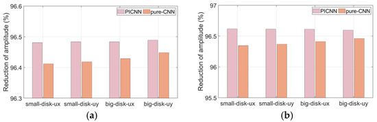
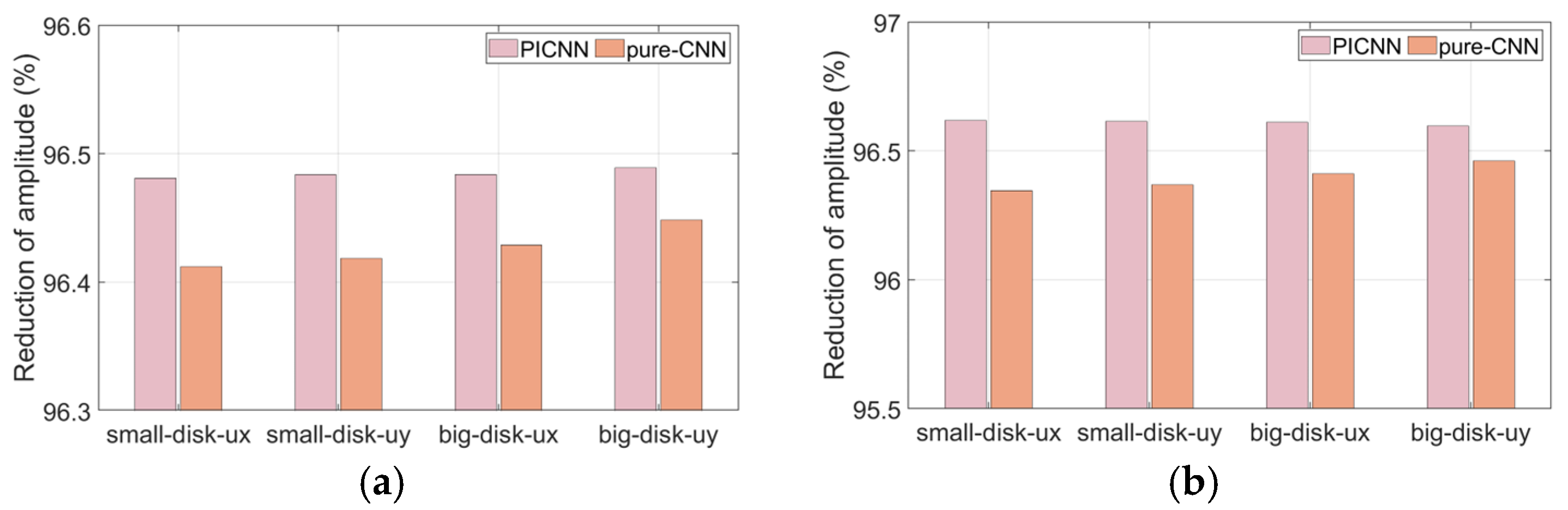
From Figure 22, we can see that the errors from the PICNN are generally lower than those from other methods except for the phase results when the small disk (or the big disk) dominates. When the small disk dominates, although the identification error of small-disk-pha from PICNN is slightly higher than that from pure-CNN (4.51% vs. 3.91%), the error of small-disk-amp from PICNN is lower (0.816% vs. 2.05%); a similar contrast presents in the results when the big disk dominates. To more directly demonstrate the strength of the PICNN, the measurement response reductions after balancing are given in Figure 23, proving that the unbalance identification performance of the PICNN is still superior.

Figure 23. The response reduction based on different methods: (a) when the small disk dominates and (b) when the big disk dominates.

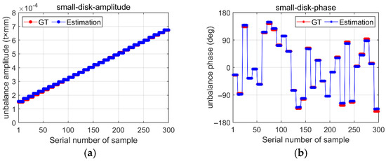
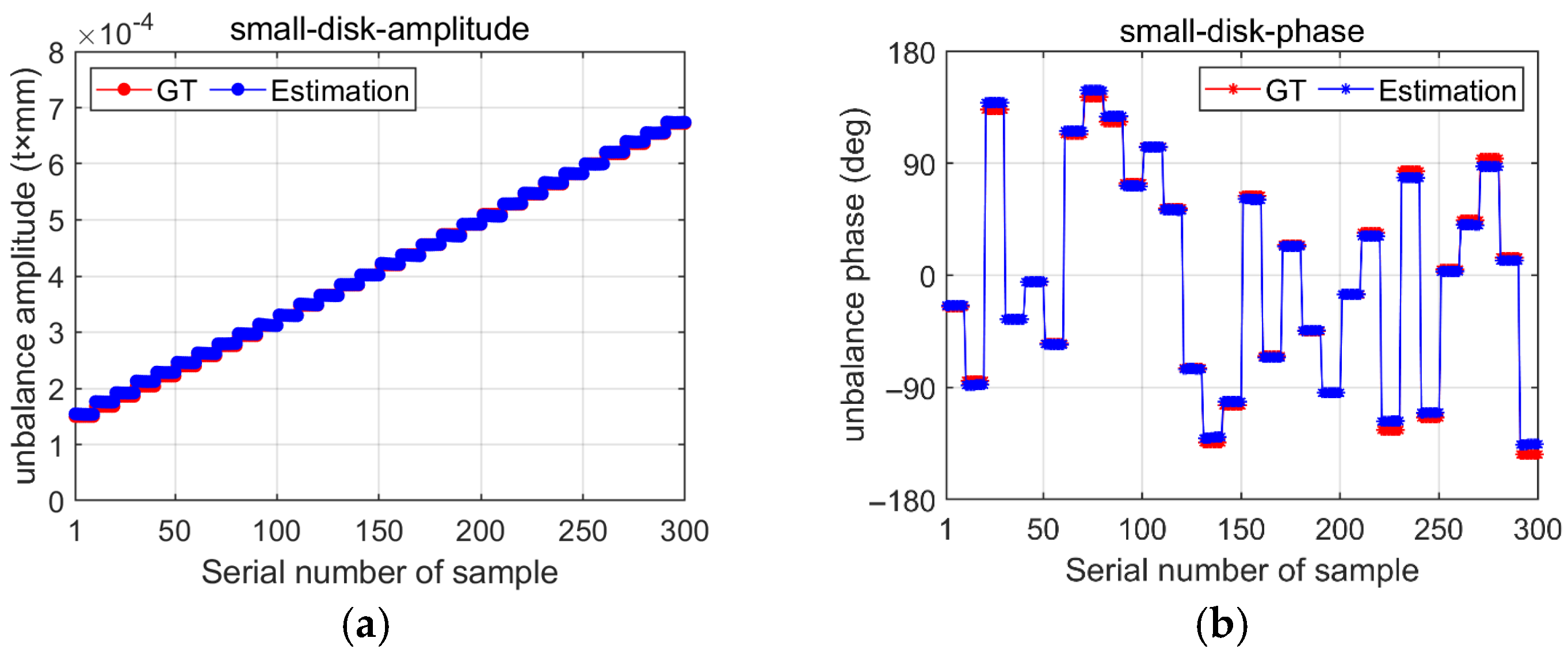
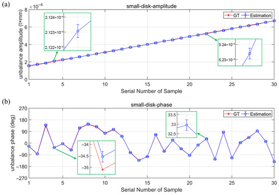
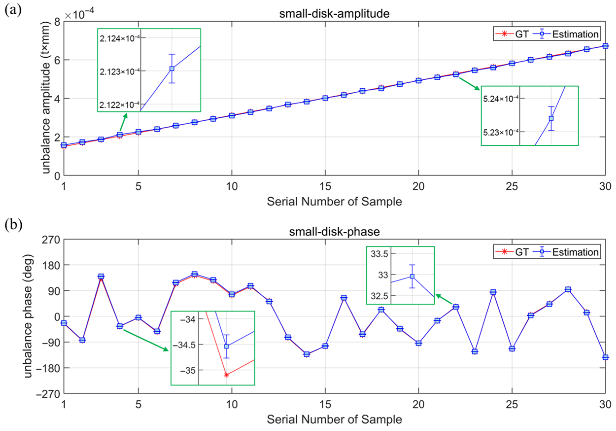
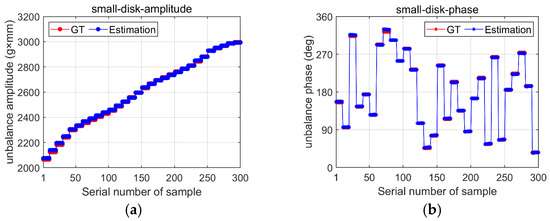
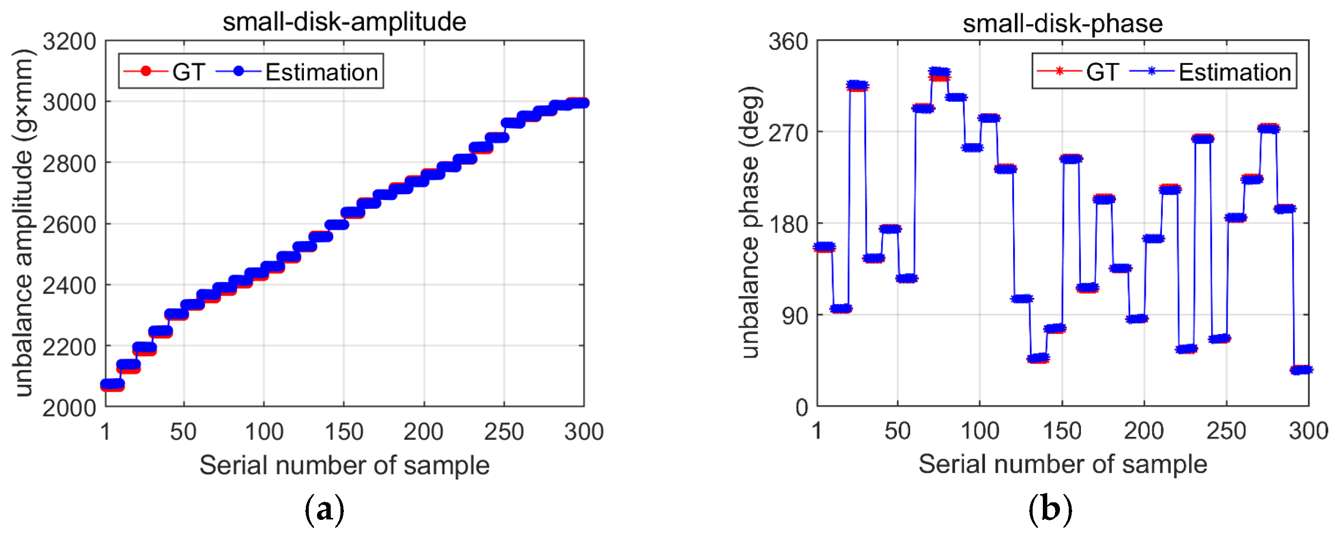
In addition to relative error, the mean and standard deviation (std) are adopted as criteria to evaluate the PICNN identification results. When the small disk dominates, the testing set comprises 30 unbalance modes, as detailed in Table A1. According to the dataset arrangement strategy, 10 samples corresponding to the same unbalance mode are set, and they share the same output. Thus, the stability of PICNN is assessed based on the mean and std of outputs for these samples. In Figure 24, each estimation result represents the mean and std of the 10 samples under the same unbalance mode. The estimation results show strong agreement with the ground truth, and the minimal std demonstrates the stability of PICNN.

Figure 24. The mean and std of the identification results when the small disk dominates: (a) the small-disk-amplitude results and (b) the small-disk-phase results.

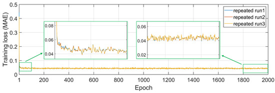
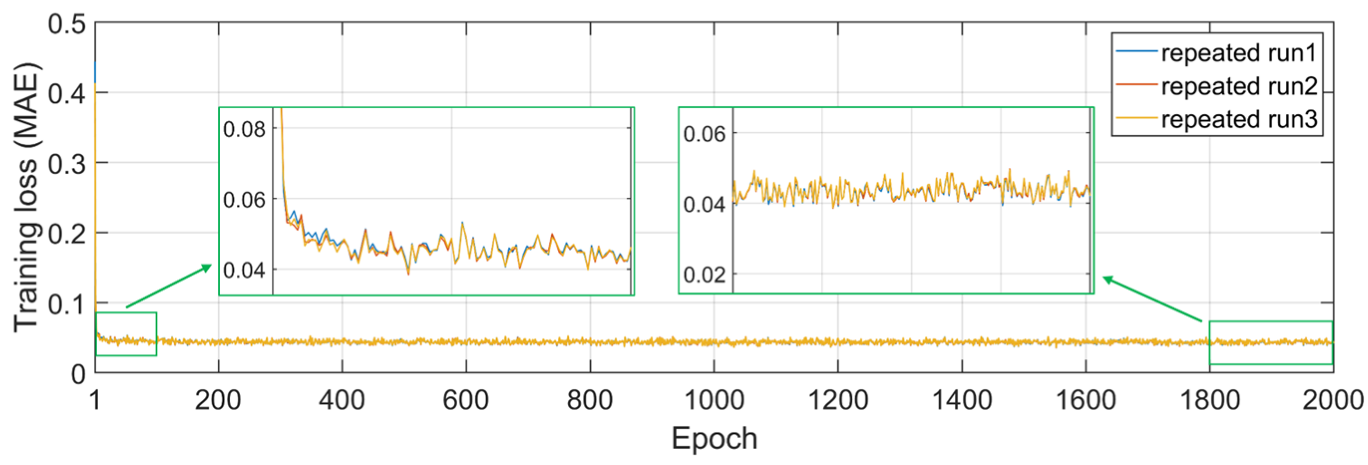
When the small disk dominates, the training losses of the PICNN during three repeated runs are compared, as shown in Figure 25. Although the random seed is fixed (see details in Section 2.3), there are still some random factors in PyTorch that generate a slight difference among repeated runs. Figure 25 can demonstrate the reliability of the PICNN identification results. More details are available through the open-access link at the end of this paper.

Figure 25. The comparison of training loss among three repeated runs.

4. Experimental Case

4.1. Test Rig and Data Collection

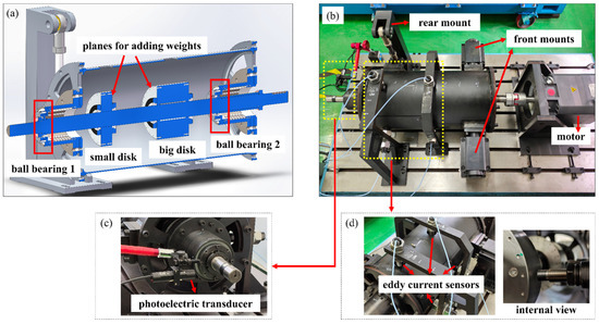
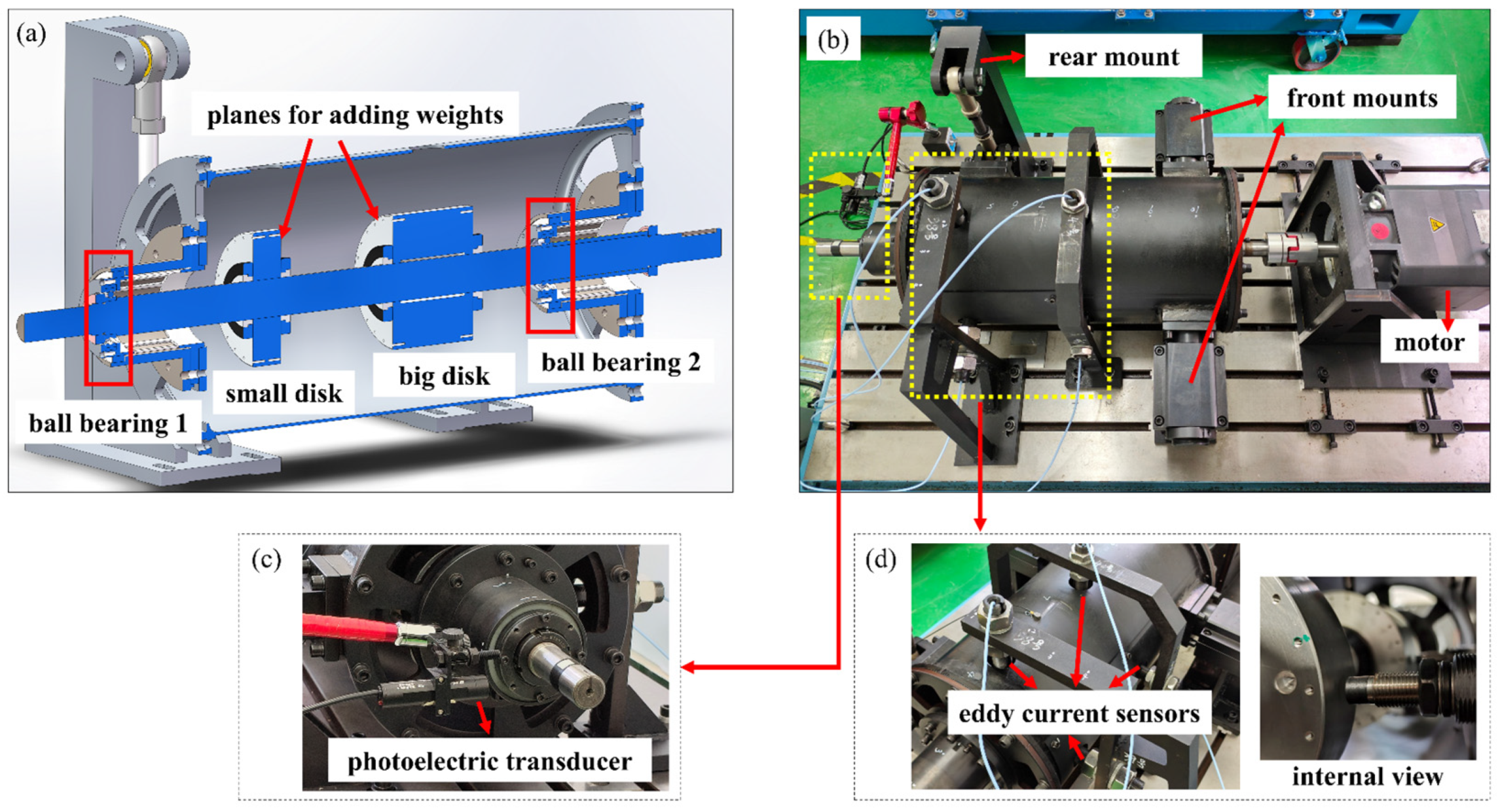
As shown in Figure 26, a twin-disk rotor-bearing-casing test rig is established to verify the performance of the proposed PICNN method. Different from the rotor-bearing bench in most of the literature, the casing is considered to be closer to the actual on-wing status. The engine mounting structures primarily result in the anisotropic supporting stiffness. Inspired by typical mounting design strategies [22,23], the experimental setup incorporates three mounts. The rear mount is in the form of a hinge joint and allows the horizontal displacement of the system. The two front mounts exert full constraints on the system. Those mounts result in the anisotropic supporting stiffness. The twin-disk rotor is supported by two ball bearings. Both supports are elastic. A flexible coupling connects the electric motor and the shaft. The length of the shaft is 870 mm. The diameter of the journal is 35 mm. The inner and outer diameters of the disks are 40 mm and 140 mm, respectively. The distance between the shaft center and the hole center (holes for adding weights) is 65 mm. The thickness of the small disk is 35 mm, and that of the big disk is 100 mm. Different weights are added to the disks to generate different unbalance configurations.

Figure 26. The test rig and data-collection devices: (a) the cross-section view of the test rig; (b) the global view; (c) the photoelectric transducer; and (d) the eddy current sensors.

Here, the measurements include the pulse signal (from the photoelectric transducer) and four displacement signals (from the eddy current sensors). The probes penetrate through the casing (Figure 26d) to measure the horizontal and vertical displacement of disks. The eddy current sensors are powered by a 24 V DC stabilized power supply, which provides stable output signals. Repeated trials under identical unbalance conditions show that the variation in measured response amplitudes remains below 0.0005 mm, while the maximum absolute response amplitude exceeds 0.2 mm. Thus, measurement errors have a negligible impact on the input samples. The sampling frequency is 50 kHz. The rotating speed is 3240 rpm. The 24 V DC stabilized power supply employs the product WPS305B from Shenzhen WANPTEK Electronic Technology CO., LTD, Shenzhen, China. The photoelectric transducer employs the product DH5640 from Jiangsu DONGHUA Testing Technology CO., LTD, Jiangsu, China. The eddy current sensors employ the product ZH21 from Zhuzhou ZhongHang Technology Development CO., LTD, Zhuzhou, China.

Before presenting the experimental identification results, several distinctive signal features should be noted. The comparison between the original experimental signals and the preprocessed ones is shown in Figure 27. The preprocessing includes the pulse signal transformation and the response signal filtering. The pulse signal transformation involves converting the original triangular pulse into an equivalent square pulse, while maintaining the consistency of the rising edge. That transformation aims to avoid having too many meaningless zeros in the inputs. The response signal filtering means that all the original responses are filtered through FFT, and only the fundamental component is retained. For this test rig, the filtering can guarantee the diagnostic information is not spoiled because there are few sub-harmonic or super-harmonic components in the original experimental signals (as shown in Figure 27). Harmonics introduced by misalignment/rub may change the relation between the unbalance excitation amplitude and the fundamental component amplitude in responses. That embodies the limitation of this paper and can be discussed in future work.

Figure 27. The comparison between the original experimental signals and the preprocessed ones. (a) original experimental signals; (b) preprocessed experimental signals.

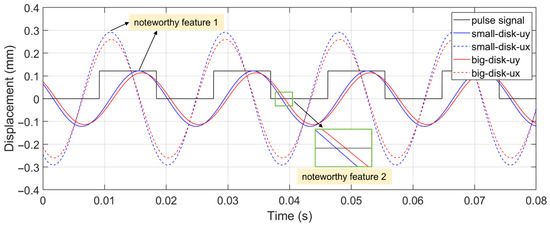
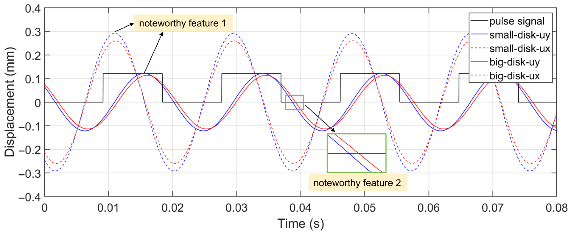
Considering that the CNN model, which is adept at image recognition, is applied to extract details from time-domain input matrices, the image-related features of the collected signals can have a strong influence on the unbalance identification performance. Taking an example where the small disk dominates, the residual responses are presented in Figure 28. The procedures of obtaining the residual responses are based on Equations (1)–(3). Noisy components are filtered through the fast Fourier transform (FFT), and only the fundamental component is retained. There are two noteworthy features. Firstly, because of the anisotropic supporting stiffness, the horizontal and vertical response amplitudes at the axially same position are different (noteworthy feature 1). Moreover, unlike the responses in Figure 20b, the response phases of small-disk-uy and big-disk-uy present a difference (noteworthy feature 2) because of the dynamic characteristics of the experiment device. Those features do not exist in some rotor benches in the open published literature [40,48,49].

Figure 28. The noteworthy features of the experimental signals when the small disk dominates.

The dataset configuration is given in Table S1 (see Supplementary Materials), where the unbalance mass is between 13.14 g and 46.68 g, and the phase is between 0.1 × $\pi$ and 1.998 × $\pi$. All of the training, validating, and testing data are from experiments. The sample leakage (e.g., the same sample appears in both training and testing sets) is avoided.

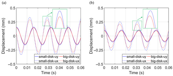
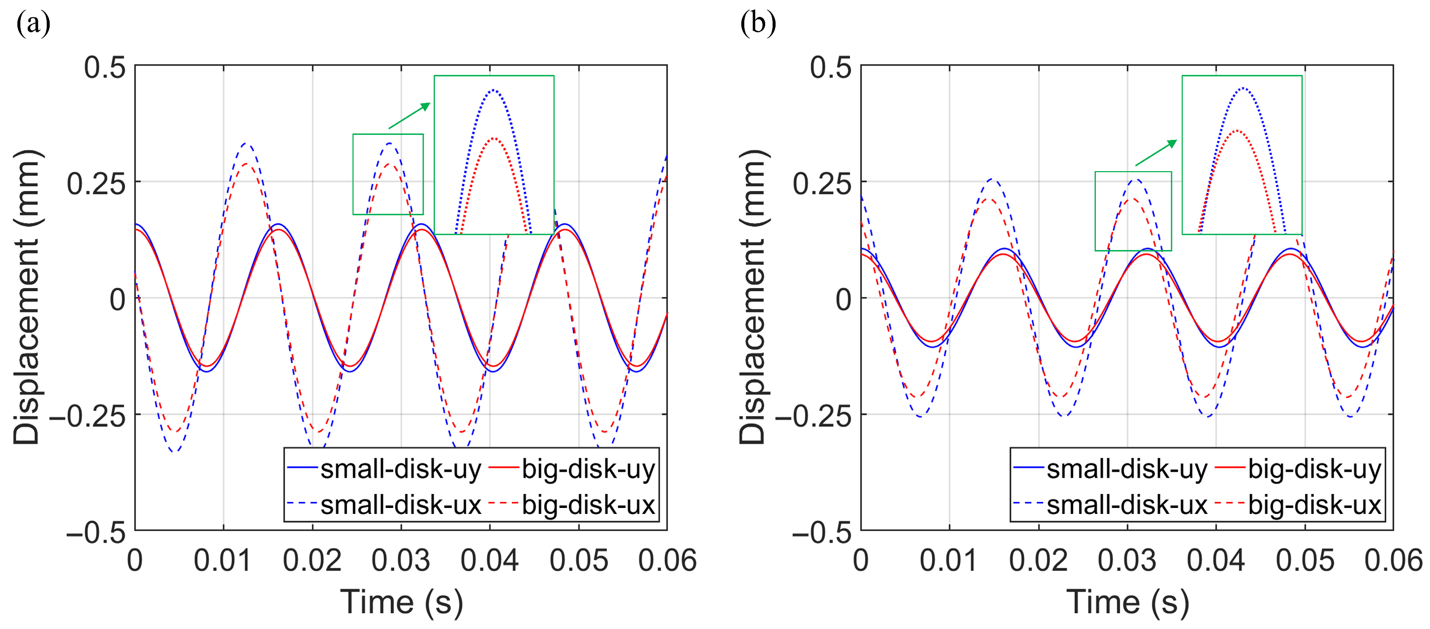
The relation between the rotor-bearing-casing simulation model and the experimental data is reflected in the PI layer of the PICNN method. It is the FRF from the simulation model that processes the collected experimental signals and outputs the judgment of the dominant faulty disk. The critical speeds of the simulation model and those of the real test rig are listed in Table 5. The relative errors are less than 5%, roughly ensuring the consistency between the simulation model and the actual system. More visibly, the simulated and experimental responses under the same unbalance excitation are presented in Figure 29. It can be seen that, not only are the amplitudes different, but the relative phases also differ. For example, as shown in the insets of Figure 29, the phase difference between “small-disk-ux” and “big-disk-ux” shows variation in the simulated and experimental responses. In the following sections, this approximate simulation model is applied to the PI layer.

Table 5. The comparison of the critical speeds between the simulation model and the test rig.

Order	Simulation Result (rpm)	Experiment Result (rpm)	Relative Error
1st	4092	4020	1.79%
2nd	4512	4740	4.81%

Figure 29. The comparison between simulated and experimental responses under the same unbalance excitation. (a) Simulated responses and (b) experimental responses.

4.2. Experimental Results

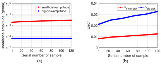
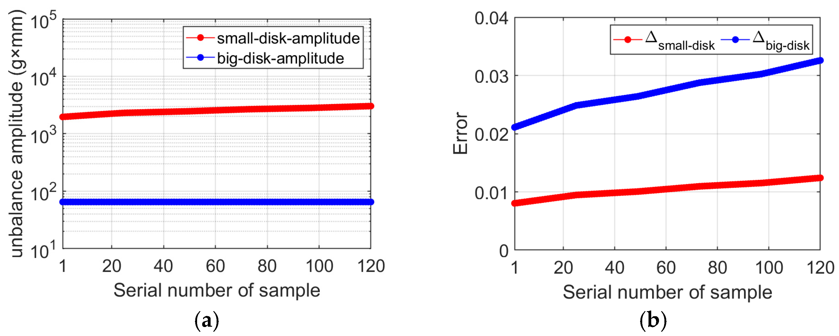
Firstly, the PI layer is triggered to conduct unbalance localization. When the small disk dominates, the outputs of the PI layer are presented in Figure 30, where 120 samples represent 120 different unbalance modes in the dataset. We can see that the criterion ${\Delta }_{big-disk}$ is more than twice as big as ${\Delta }_{small-disk}$. According to the metric in Figure 5, the small disk is determined as the dominant faulty part.

Figure 30. The outputs of the PI layer when the small disk dominates in the experimental setup: (a) the ground truth and (b) the error output from the PI layer.

When both disks dominate, the results are shown in Figure 31. In this case, the errors obtained under different assumptions are close to each other, guiding the PICNN to trigger the NN model 3 in Figure 4b.

Figure 31. The outputs of the PI layer when both disks dominate in the experimental setup: (a) the ground truth and (b) the error output from the PI layer.

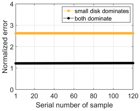
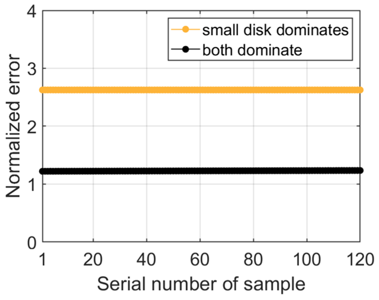
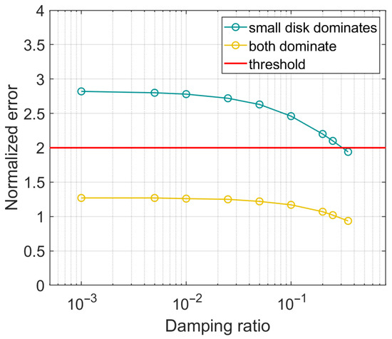
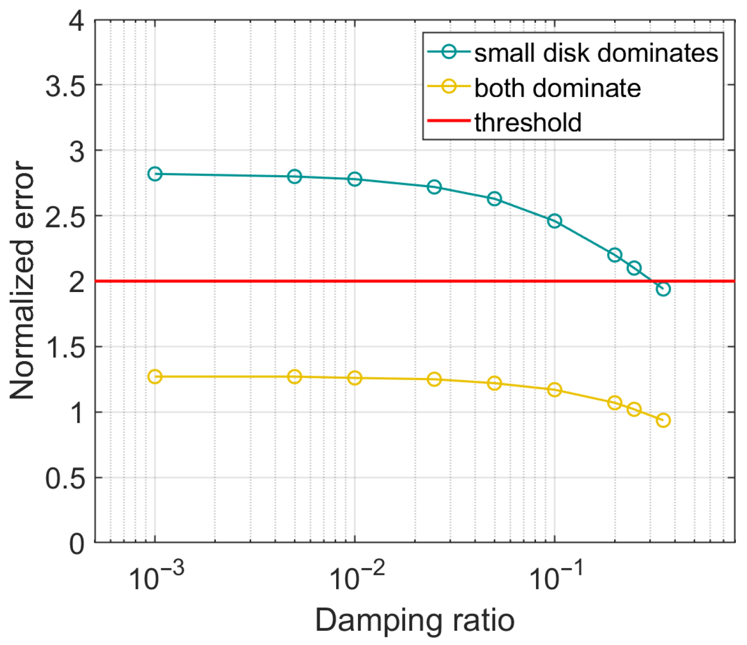
A normalized comparison is shown in Figure 32. Here, the normalized error is calculated by ${\Delta }_{big-disk}/{\Delta }_{small-disk}$. The results for “both dominate” are based on the first 120 samples in Figure 31b. When only the big disk dominates, the performance is similar to what is achieved in the case of when the“small disk dominates”. As shown in Figure 32, the normalized error is near 1 in the case of “both dominate”, while that value is far over 2 for the “small disk dominates”. That distinct difference can demonstrate the reliability of triggering the correct sub-network. Again, it is noteworthy that the PI layer does not require a high-fidelity simulation model; just a rough one will do.

Figure 32. A normalized comparison of the outputs from the PI layer under different fault modes.

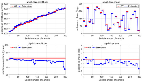
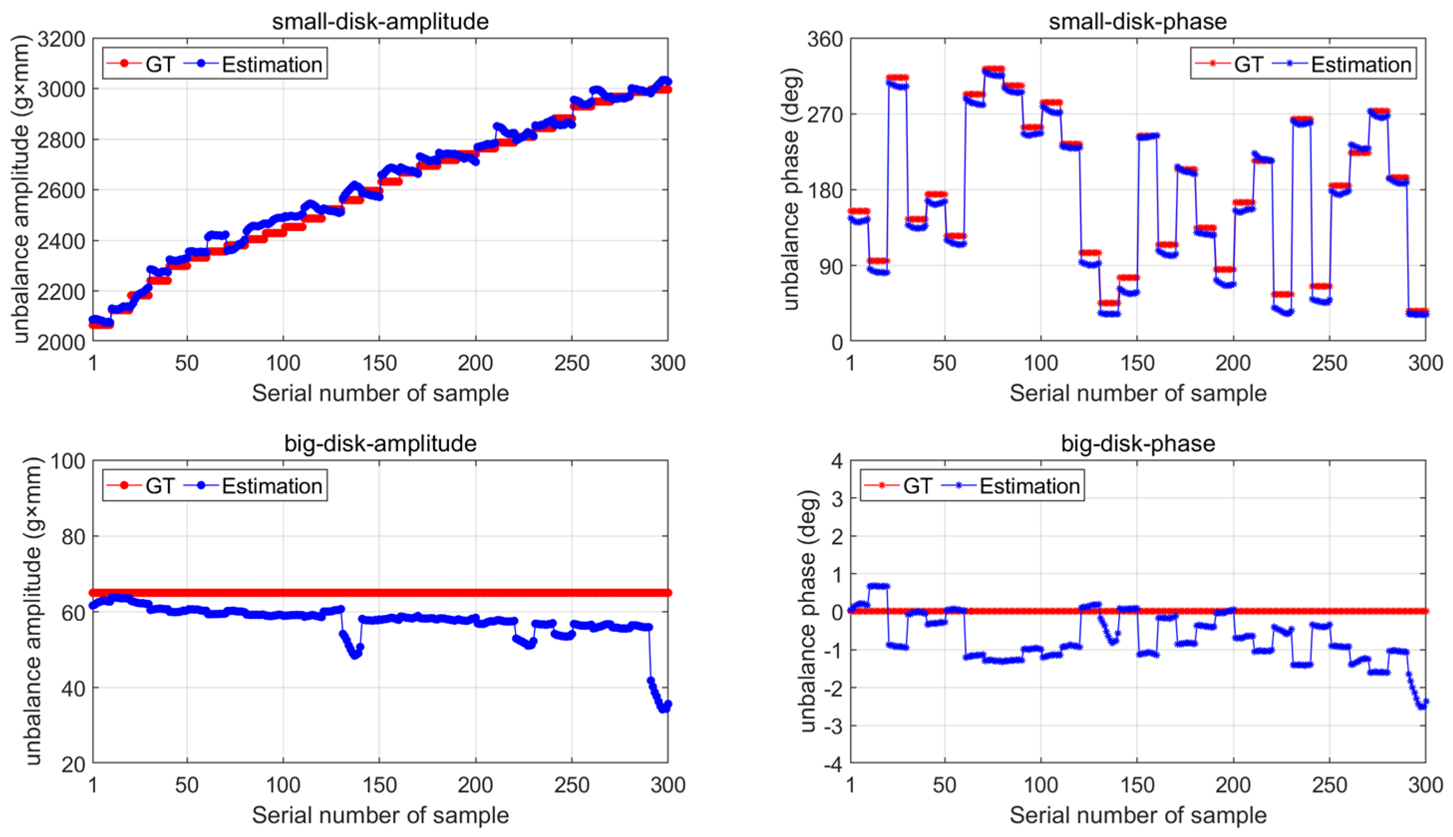
Following the isolation, the identification results when the small disk dominates are provided in Figure 33. The relative error for the amplitude is only 0.228%, while the value for the phase is 0.824%.

Figure 33. The identification results from the PICNN when the small disk dominates in the experimental setup. (a) unbalance amplitude results; (b) unbalance phase results.

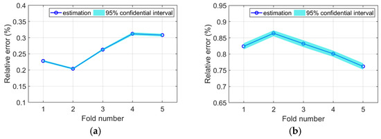
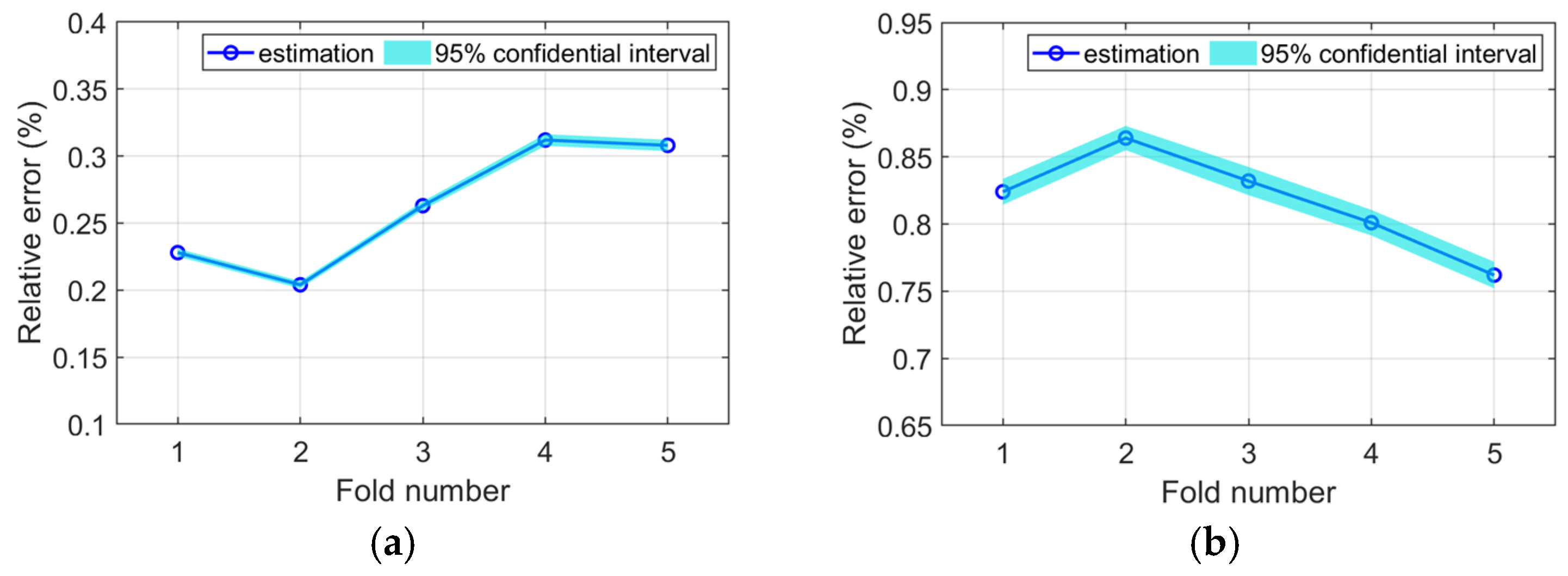
Furthermore, the five-fold cross-validation is conducted, with 95% confidential intervals evaluated through the Monte Carlo (MC) dropout method. As shown in Figure 34, the fluctuation across different folds is small. All relative errors of unbalance amplitudes are less than 0.35%, and those for unbalance phases are consistently below 0.90%. The confidential intervals are narrow, with widths generally around 3.0% of their respective central values.

Figure 34. The identification results with confidential intervals under the 5-fold cross-validation: (a) unbalance amplitude and (b) unbalance phase.

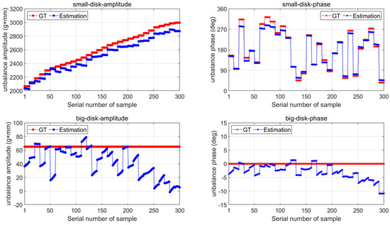
An ablation study comparing different kernel sizes is also conducted. As shown in Table 6, the identification performance is virtually insensitive to the kernel size.

Table 6. The ablation study comparing different kernel sizes.

Kernel Size	Unbalance Amplitude		Unbalance Phase
	Relative Error (%)	95% Confidential Interval	Relative Error (%)	95% Confidential Interval
50 × 5	0.228	[0.225, 0.231]	0.824	[0.814, 0.834]
60 × 5	0.262	[0.255, 0.269]	0.872	[0.848, 0.896]
70 × 5	0.253	[0.246, 0.260]	0.856	[0.833, 0.879]

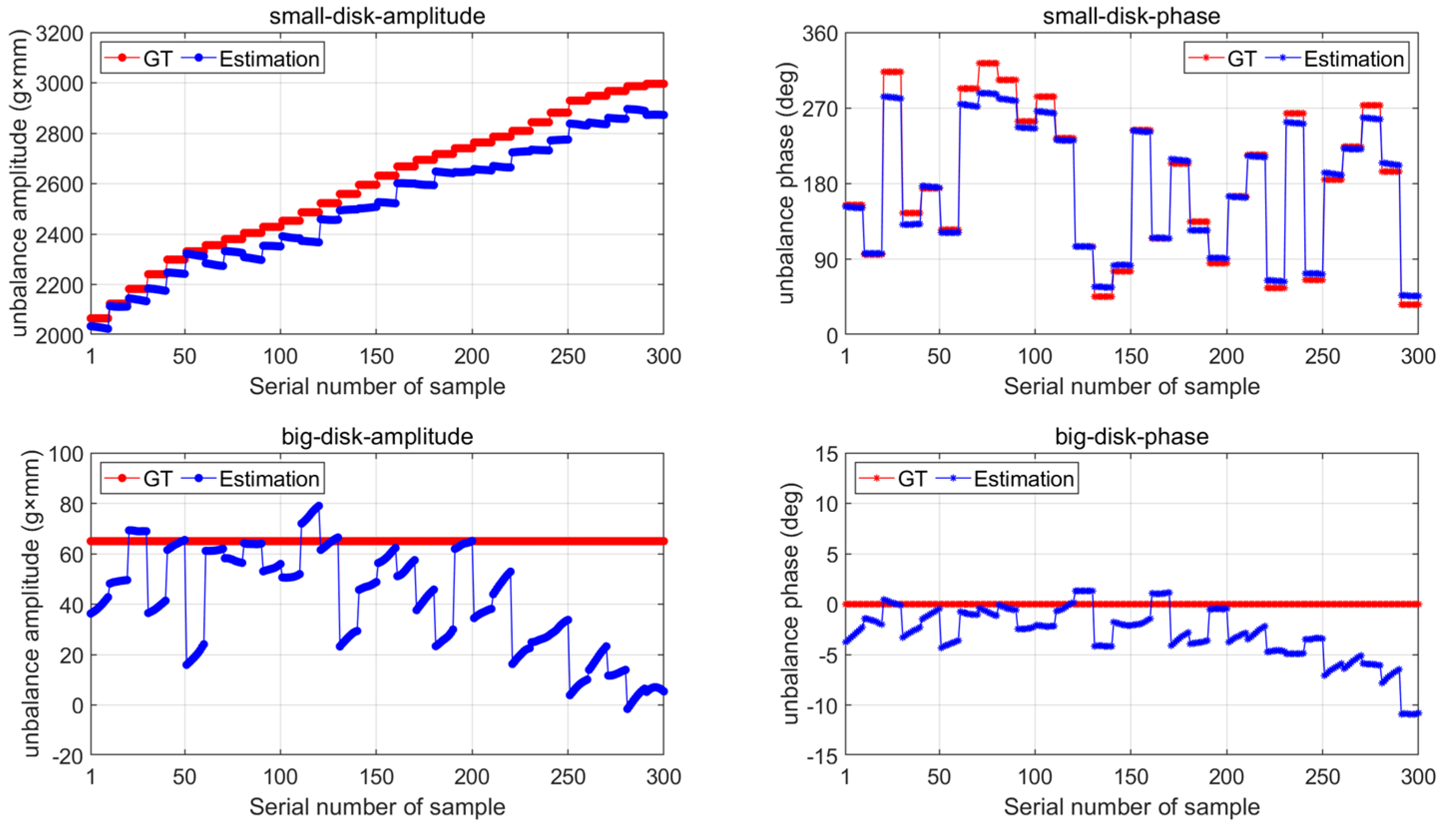
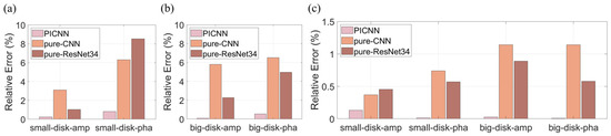
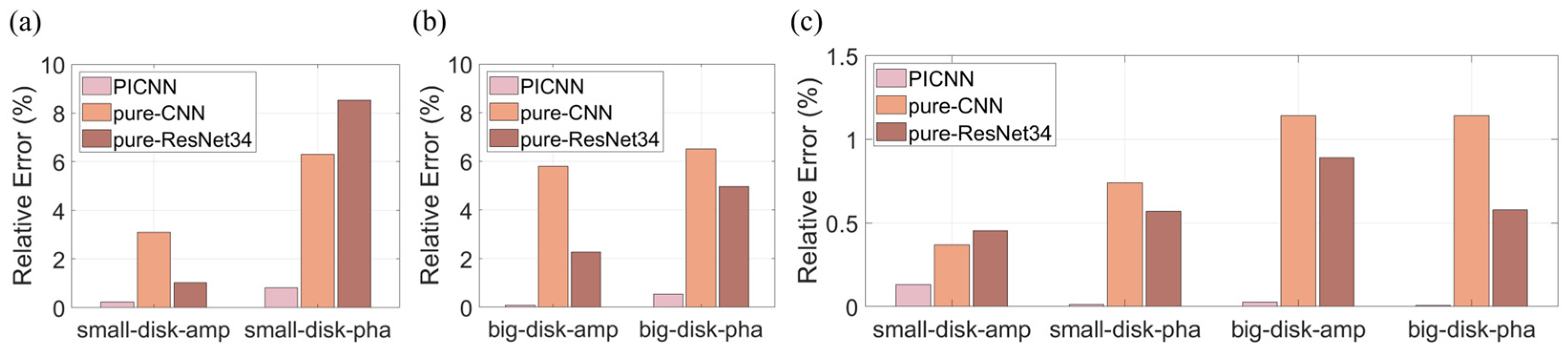
The results from the pure-CNN and the pure-ResNet34 are given in Figure 35 and Figure 36, respectively. Through the comparison among Figure 33, Figure 35 and Figure 36, it is apparent that the results from the PICNN stand out for the highest precision. The phenomenon here is similar to what we find in the simulation datasets. That is to say, the insignificant parameters can be the encumbrances for identifying the dominant unbalance amplitudes and phases. The comparison under different fault modes is provided in Figure 37. The reason why the PICNN achieves better results in experimental datasets than simulation datasets can be the noteworthy feature 2 marked in Figure 28, which does not exist in the simulation datasets. Moreover, the proportion of the horizontal amplitude to the vertical amplitude is bigger than that in the simulation model. Considering that the CNN model is noted for its capability in image recognition, the enrichment of the input may further improve the mapping performance. Taking the small-disk-amp in Figure 37a as an example, in contrast to its counterpart in Figure 22a, the relative errors of all three methods drop by a certain degree.

Figure 35. The identification results from the pure-CNN when the small disk dominates in the experimental setup.

Figure 36. The identification results from the pure-ResNet34 when the small disk dominates in the experimental setup.

Figure 37. The comparison among different methods applied in the experimental setup: (a) when the small disk dominates, (b) when the big disk dominates, and (c) when both dominate.

5. Discussion

5.1. Effect of the Model Precision on the PI Layer

In this section, the robustness of the PI layer is discussed. In engineering practice, determining highly precise values for the stiffness and damping parameters in the simulation model remains challenging. That limitation mainly lies in two aspects. First, it is difficult to accurately characterize and model the real mechanical states of multiple components after assembly. Second, the occurrence of structural damage in the rotor unbalance system can change the original characteristics of the system. In that case, it is necessary to assess the unbalance identification methods when the stiffness and damping vary.

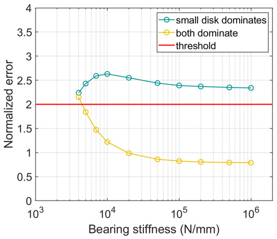
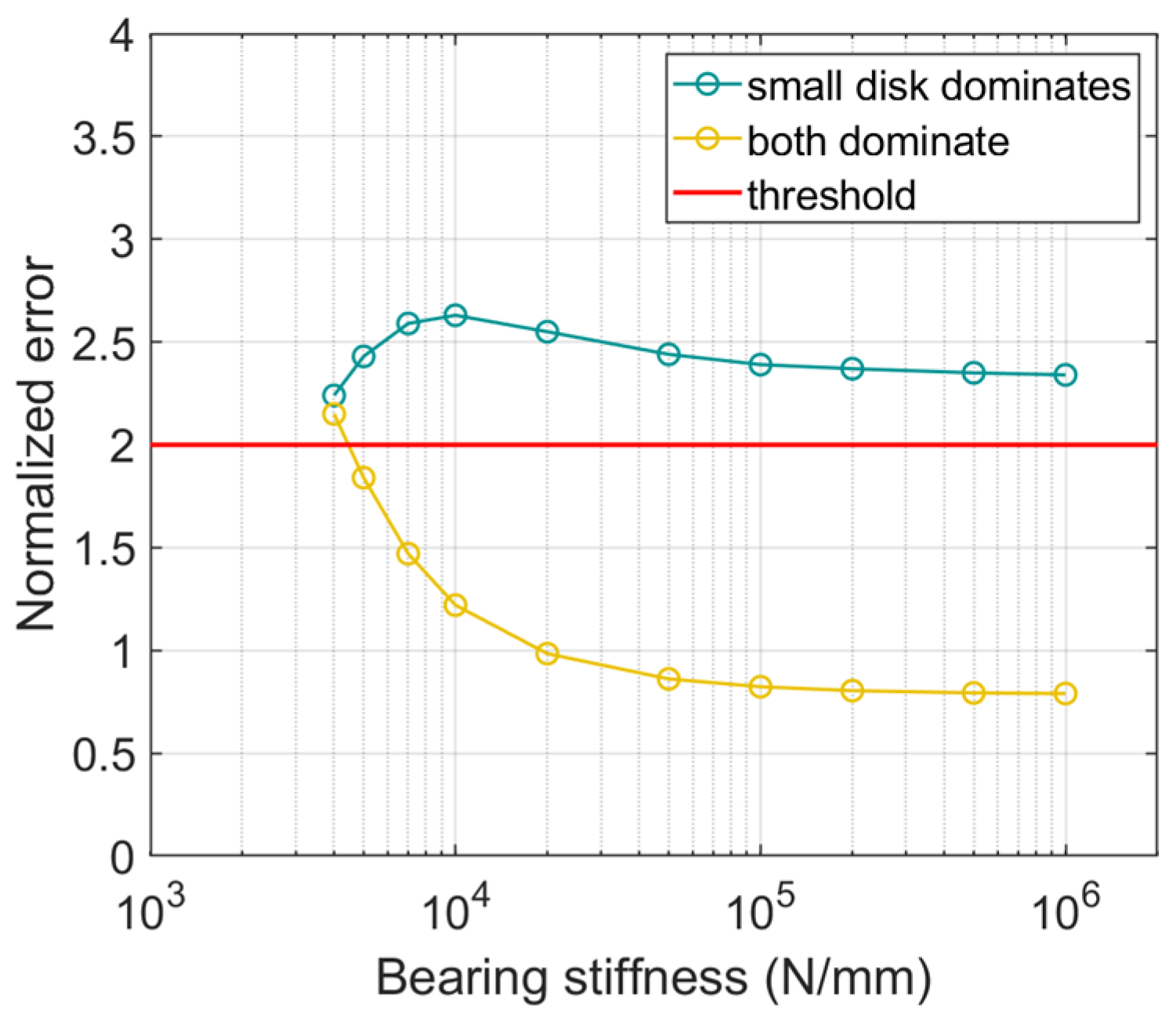
The effects of the bearing stiffness, mount stiffness, and the damping ratio on the PI layer are discussed here. Firstly, the robustness against bearing stiffness is presented. Figure 38 presents the normalized errors output from the PI layer under different bearing stiffness. The stiffness 1 × 10⁴ (N/mm) generates the best fit between the simulation model and experiment setup in terms of critical speeds. For clarity, let us refer to the failure mode in which the small disk dominates as mode 1, and the failure mode in which both disks dominate as mode 3. In Figure 38, the threshold is set to 2, which means the errors for mode 1 are required to be greater than 2, and the errors for mode 3 are required to be less than 2. When the stiffness ranges from 4.5 × 10³ to 1.0 × 10⁶ (N/mm), the normalized errors for mode 1 remain above the threshold, while the results for mode 3 stay below the threshold. This demonstrates the robustness of the PI layer against stiffness discrepancies and provides a practical design guideline: the allowable deviation in bearing stiffness lies within [4.5 × 10³, 1 × 10⁶] (N/mm). Some typical results are also listed in Table 7 and Table 8. In Table 7, “Err-1st-order” means the relative error between the simulation value and the experimental value at the first critical speed. The experimental critical speeds at the first two modes are 67 Hz and 79 Hz, respectively. In Table 8, the experimental results for the mode shape in the x (horizontal) and y (vertical) directions are 1.158:1 (small disk to big disk) and 1.160:1, respectively.

Figure 38. The normalized error outputs from the PI layer under different bearing stiffness.

Table 7. The first two critical speeds of the simulation model under different bearing stiffness.

Stiffness (N/mm)	1st-Order (Hz)	2nd-Order (Hz)	Err-1st-Order (%)	Err-2nd-Order (%)	Err-Mean (%)
7 × 103	66.6	72.6	0.60%	8.1%	4.4%
1 × 104	68.2	75.2	1.8%	4.8%	3.3%
1 × 105	71.7	81.4	7.0%	3.0%	5.0%

Table 8. The mode shapes under different bearing stiffnesses.

Stiffness (N/mm)	Mode Shape ux (Small Disk:Big Disk)	Mode Shape uy (Small Disk:Big Disk)	Err-ux (%)	Err-uy (%)
7 × 103	1.179:1	1.121:1	1.8%	3.4%
1 × 104	1.204:1	1.145:1	4.0%	1.3%
1 × 105	1.257:1	1.193:1	8.5%	2.8%

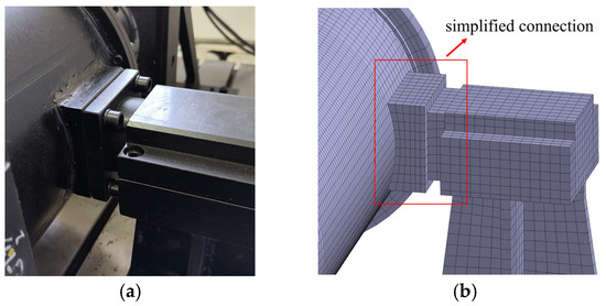
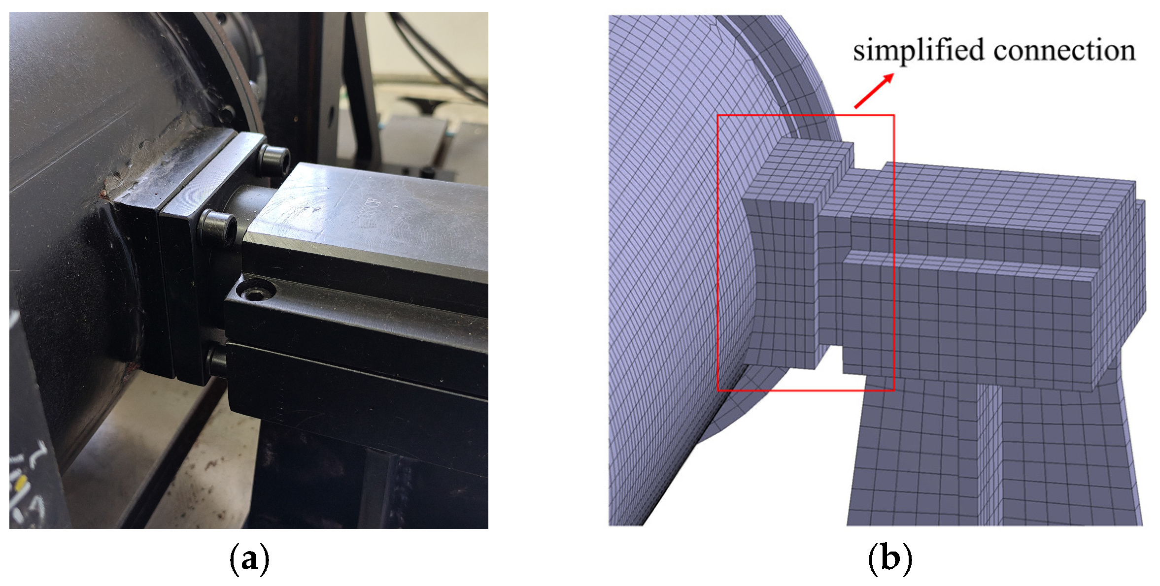
Secondly, the sensitivity to variations in mounting stiffness is further investigated. As shown in Figure 39, the front mount-to-casing connection is simplified in the finite element model (FEM). This simplification can result in the mounting stiffness discrepancy between the actual test rig and the FEM. Different elastic moduli of the front mount-to-casing connection elements are applied to achieve different mount stiffness. The material of the connection is a kind of carbon structural steel, with the elastic modulus design value of 200 GPa. When this value varies from 100 GPa to 300 GPa, the resulting changes are listed in Table 9. In Table 9, the response anisotropy is obtained under the unbalance amplitude of 1.07 × 10³ (g × mm) at the small disk.

Figure 39. The connection between the front mount and the casing. (a) Actual connection in the experimental setup and (b) simplified connection in the FE model.

Table 9. The resulting changes under different elastic moduli.

Elastic Modulus (GPa)	1st-Order (Hz)	2nd-Order (Hz)	Small-Disk Response Anisotropy (uy:ux)	Big-Disk Response Anisotropy (uy:ux)
100	65.2	74.9	1:1.82	1:1.68
150	67.1	75.1	1:1.61	1:1.51
200	68.2	75.2	1:1.51	1:1.43
250	68.9	75.2	1:1.44	1:1.38
300	69.4	75.3	1:1.40	1:1.35

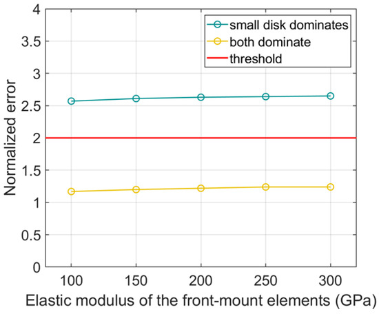
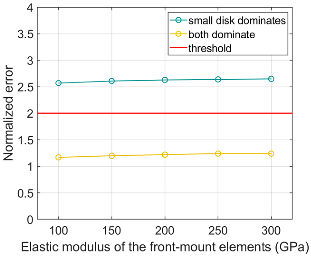
As listed in Table 9, with the increase in the front mount-to-casing connection stiffness, the mount anisotropy tends to decrease, resulting in smaller response anisotropy. Facing different mount anisotropies in the FEM, the PI layer outputs normalized errors, presented in Figure 40. The input sample is from the test rig, and the FRF-based PI layer is from FEMs of different mount anisotropies. It can be seen from Figure 40 that, although different degrees of discrepancy between the test rig and the FE model exist, none of the outputs violates the threshold, demonstrating the robustness of the PI layer against mount stiffness. The results in this part can be summarized as a practical design guideline. In terms of the front mount-to-casing connection stiffness, the investigation verifies a feasible deviation range of $\pm 50\%$, which is promising for practical application.

Figure 40. The normalized error outputs from the PI layer under different mount stiffnesses.

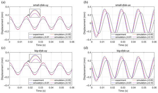
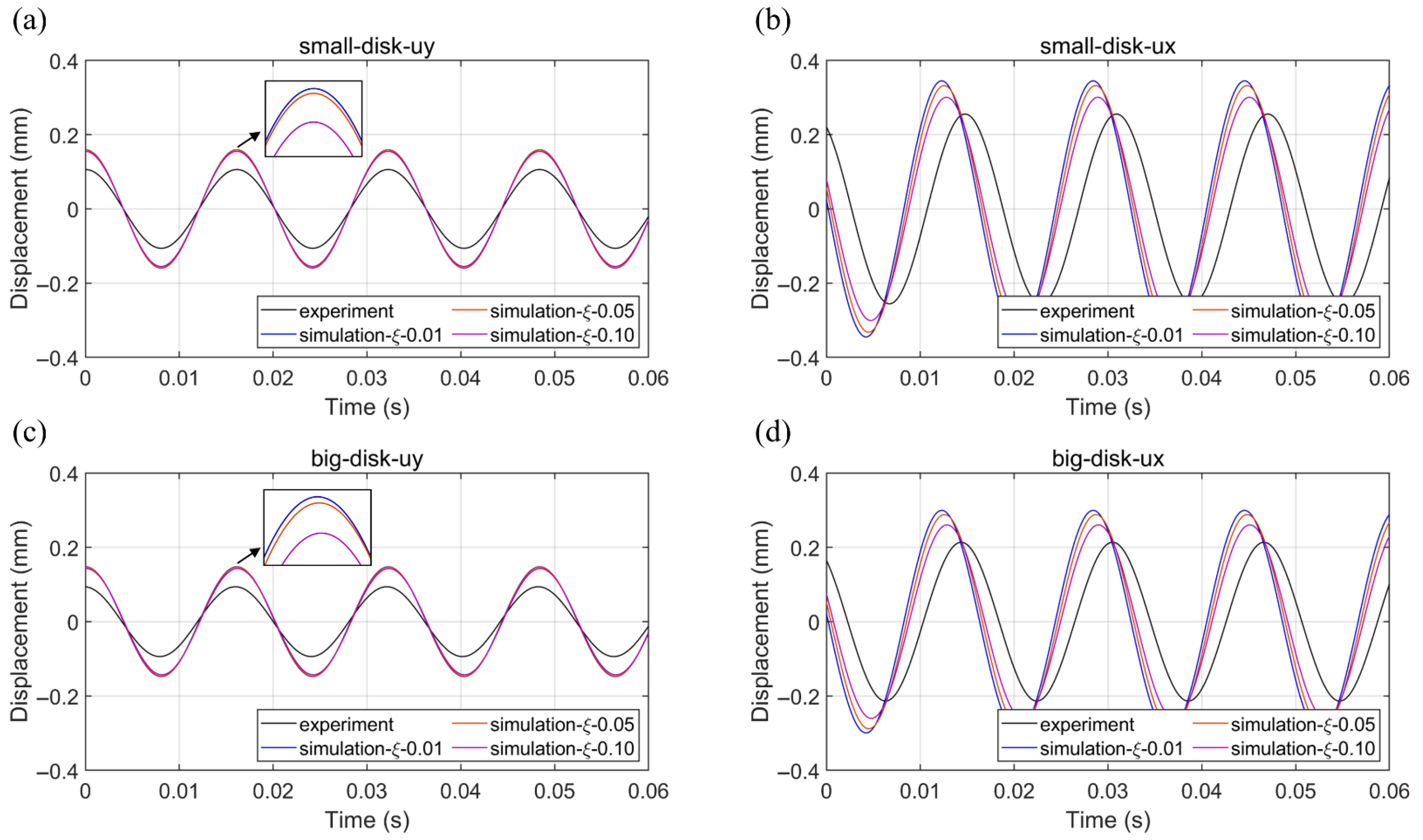
Thirdly, the effect of the damping ratio is further discussed. The damping ratio means the parameter $\xi$ in the Rayleigh damping C, where $\mathit{C}=\alpha \mathit{M}+\beta \mathit{K}$, $\alpha =\left(2{\omega }_i{\omega }_j\xi \right)/\left({\omega }_i+{\omega }_j\right)$, and $\beta =\left(2\xi \right)/\left({\omega }_i+{\omega }_j\right)$. The parameters ${\omega }_i,{\omega }_j$ here are 428.3 and 472.3, respectively. The damping matrix in this paper only includes the Rayleigh damping and the gyroscopic effect. The differences between simulated and experimental responses under the same unbalance excitation are presented in Figure 41. It can be seen that the amplitudes and phases of the simulated measurement are not consistent with the experimental results. Facing that challenge, the outputs from the PI layer are presented in Figure 42.

Figure 41. The comparison between simulated and experimental responses under the same unbalance excitation. (a) Small-disk-uy; (b) small-disk-ux; (c) big-disk-uy; and (d) big-disk-ux.

Figure 42. The normalized error outputs from the PI layer under different damping ratios.

According to the results in Figure 42, the lower bound of the tolerance range is below 1 × 10⁻³, while the upper bound is 0.30. This broad tolerance range demonstrates the robustness of the PI layer against damping ratio discrepancies.

5.2. Effect of Different Levels of Noise

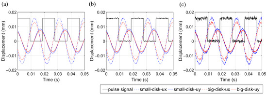
In this section, the time-domain input signals are subject to different levels of noise. A direct comparison of inputs under various signal-to-noise ratios (SNRs) is presented in Figure 43. Here, the noise injection is in time responses obtained from the rotor-bearing-casing system in the previous numerical case. When the SNR reaches 25 dB, the time-domain waveform distortion is remarkable, especially for the response phase (the phase by which the displacement peak lags behind the pulse rising edge). The response phase has shifted by 6° to 8° under the noise interference. Considering that the phase variation among different testing samples is only 12°, this disparity has already posed a great challenge for unbalance phase identification.

Figure 43. The input signals under different SNRs: (a) 70 dB; (b) 35 dB; and (c) 25 dB.

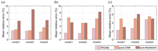
The identification results from the PICNN and the benchmark models are compared in Figure 44. Here, for simplification, modes 1, 2, and 3 are used to represent when the small disk dominates, the big disk dominates, and both dominate, respectively. The mean relative error is the mean of the relative errors achieved on unbalance amplitudes and phases of dominant disks. As shown in Figure 44, the proposed PICNN achieves the lowest error compared to other methods, demonstrating its strength in anti-noise.

Figure 44. The comparison among different methods under different SNRs: (a) 70 dB; (b) 35 dB; and (c) 25 dB. Modes 1, 2, and 3 represent when the small disk dominates, the big disk dominates, and both dominate, respectively.

5.3. Effect of Sensor Placement Errors

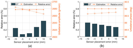
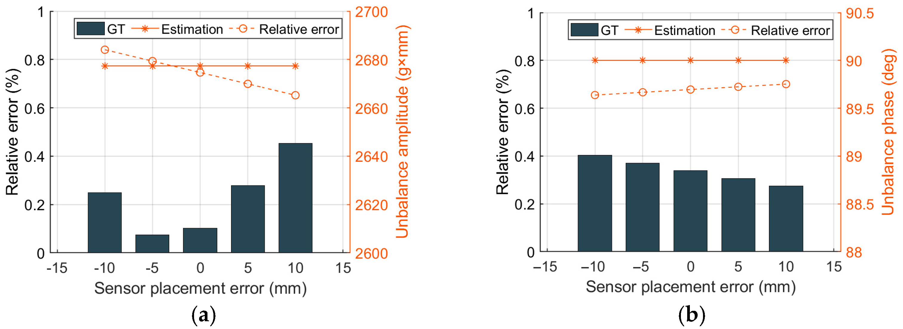
In this section, the effect of sensor placement errors is further discussed. In practice, the actual sensor placements can be different from those involved in the datasets. The effect of the placement errors on the identification performance is shown in Figure 45. The sensor placement error in Figure 45 means the deviation occurs in the small-disk measurement from its ideal axial position. The identification results in Figure 45 are from the PICNN trained on the experimental datasets under the rotating speed of 54 Hz. In view of the fact that the axial thickness of the small disk is 35 mm, the considered deviation from the ideal position (disk center) ranges from −10 mm to 10 mm. The effect of the sensor placement error on the PI layer is tiny, resulting in changes of less than 0.1%. As shown in Figure 45, the relative errors of the identified unbalance amplitudes and phases are all less than 0.5%. The reason why the result under the sensor placement error of 0 does not achieve the lowest relative error is that Figure 45 typically presents the influence under one specific unbalance mode, while the trained PICNN accommodates 60 different unbalance modes.

Figure 45. The identification results under different sensor placement errors. (a) Unbalance amplitudes and (b) unbalance phases.

5.4. Comparison with the Model-Based Method

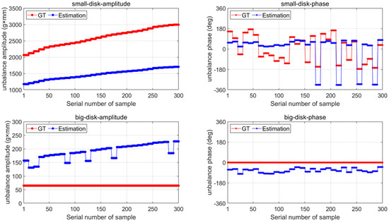
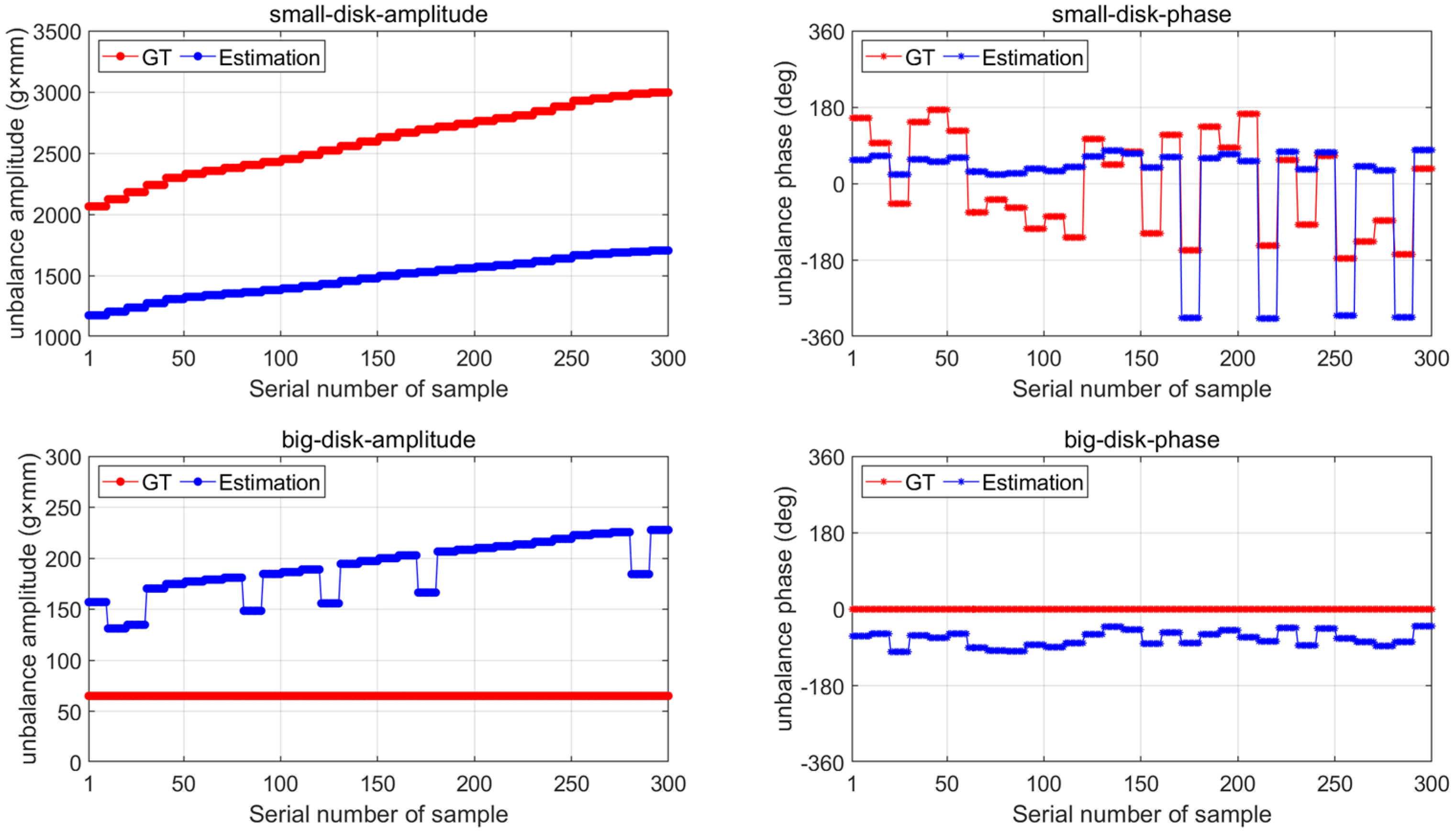
In this section, the comparison with the classical model-based influence coefficient method (ICM) in the same setup is further investigated. Here, the entailed influence coefficients are obtained by virtually applying trial weights on the small disk and the big disk in the FEM, which is a typical approach when the ICM is put into practice [50,51,52]. When the small disk dominates, the identification results from the ICM are shown in Figure 46. In contrast to the PICNN results in Figure 33, the errors in Figure 46 are noticeable. The relative error of small-disk amplitude is 43.1%, and that of small-disk phase is 88.8%. Additionally, it is noteworthy that, although the ICM yields results with limited accuracy, it can qualitatively distinguish the dominant disk. The estimated unbalance amplitudes of the small disk are nearly ten times those of the big disk. This finding, from another perspective, demonstrates that the simulation model consistent with the actual setup in modal characteristics can effectively achieve unbalance localization, without the need for a high-fidelity model generating identical responses.

Figure 46. The identification results from the ICM when the small disk dominates.

5.5. Performance Under Different Rotating Speeds

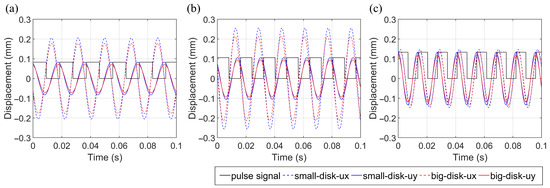
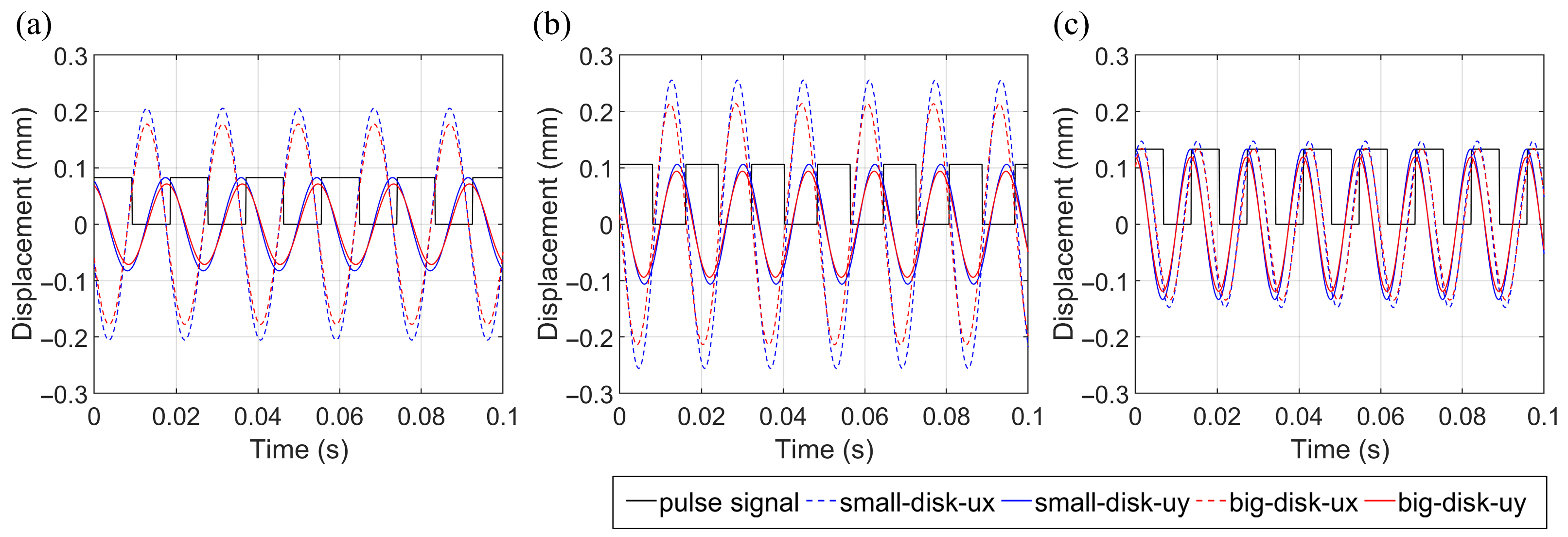
In this section, the performance of the PICNN under different rotating speeds is demonstrated. The operating conditions where the rotating speed is below, near, or above (54 Hz, 62 Hz, 73 Hz, respectively) the first-order critical speed (67 Hz) are all considered. Here, the time responses are all collected from the test rig, shown in Figure 47. The PICNN is retrained for each speed. This section focuses on the challenges related to the variation in time-domain waveforms. Firstly, the number of periods included in the given time length is different. The higher the rotating speed, the denser the waveform is. Secondly, not only do the absolute amplitudes of measurements change with the rotating speeds, but the relative amplitudes between each other also vary. Since the time-domain signals directly constitute the input samples, the above waveform-related challenges can have a direct impact on the PICNN performance.

Figure 47. The time-domain inputs under different rotating speeds: (a) 54 Hz; (b) 62 Hz; and (c) 73 Hz.

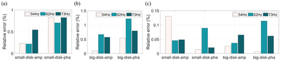
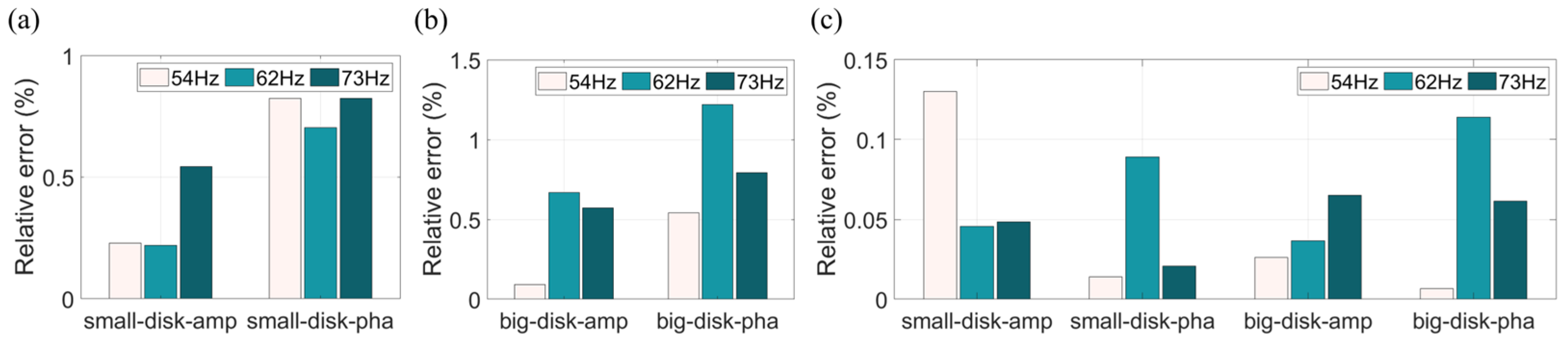
The outputs from the PI layer are similar to Figure 32. The identification precision from the PICNN is presented in Figure 48. The involved datasets are listed in Tables S2 and S3 (see Supplementary Materials). As shown in Figure 48, the PICNN can achieve great identification with the highest relative error of less than 1.5%.

Figure 48. The identification precision of the PICNN under different rotating speeds. (a) When the small disk dominates, (b) when the big disk dominates, and (c) when both dominate.

6. Conclusions

In this paper, a physics-informed convolutional neural network is proposed and applied to the unbalance localization and identification of a multi-disk rotor-bearing-casing system with anisotropic supporting stiffness. By capturing the characteristics of actual engine mounts, this system is representative of engine installation status on the UAV platform. To the best of the authors’ knowledge, little research has been done to design and experimentally verify an efficient physics-informed neural network applied to the aforementioned complex system. Both numerical and experimental cases are presented to demonstrate the strengths of the PICNN method, which can be summarized in three aspects below.

(1)

Compared to the pure-CNN methods, the proposed PICNN features in providing identification with higher precision, whose relative errors are all below 1.5% under various experimental datasets, and possesses physical interpretability.

(2)

The PI layer is based on the FRF of the simulation model. It does not require a high-fidelity model that generates responses identical to the actual ones. The robustness against modeling errors in bearing stiffness, mounting stiffness, and damping ratios is demonstrated. This greatly ensures the practicality of the proposed method.

(3)

Different from the rotor-bearing test bench in most of the literature, a twin-disk rotor-bearing-casing experimental setup with anisotropic supporting stiffness is established to get closer to the actual on-wing status. The horizontal response amplitude is more than twice that of the vertical one, which can be addressed in the proposed method.

Due to the scope of this study, more scenarios can be further investigated in future work. The extension of this PICNN framework to other specific NN models can be investigated, which are not limited to image-recognition tools. In addition, the domain adaptation across operational variabilities, temperature, and other faults can be further investigated.

References

- Kurt, E.; Arabul, A.Y.; Keskin Arabul, F.; Senol, I. Parallel hybrid propulsion system with integration of designed electric machine for medium altitude long endurance UAV. Heliyon 2025, 11, e42871. [Google Scholar] [CrossRef] [Scilit] [PubMed]
- Hung, J.Y.; Gonzalez, L.F. On parallel hybrid-electric propulsion system for unmanned aerial vehicles. Prog. Aerosp. Sci. 2012, 51, 1–17. [Google Scholar] [CrossRef] [Scilit]
- Ismail, N.; Norhashim, N.; Hamid, S.A.; Mohd Kamal, N.L.; Sahwee, Z.; Shah, S.A.; Yusoff, W.Y.W. Utilizing solar energy for UAVs: Advancements, challenges and future perspectives in defense and military applications—A review. Sol. Energy Mater. Sol. Cells 2026, 296, 114075. [Google Scholar] [CrossRef] [Scilit]
- Xiao, C.; Wang, B.; Zhao, D.; Wang, C. Comprehensive investigation on Lithium batteries for electric and hybrid-electric unmanned aerial vehicle applications. Therm. Sci. Eng. Prog. 2023, 38, 101677. [Google Scholar] [CrossRef] [Scilit]
- Zountouridou, E.; Kiokes, G.; Dimeas, A.; Prousalidis, J.; Hatziargyriou, N. A guide to unmanned aerial vehicles performance analysis—The MQ-9 unmanned air vehicle case study. J. Eng. 2023, 2023, e12270. [Google Scholar] [CrossRef] [Scilit]
- Chen, Y.; Wang, W.; Yang, C.; Liang, B.; Qin, H.; Liu, W. An efficient energy management strategy for hybrid electric unmanned aerial vehicles considering exhaust gas temperature of the turboshaft engine. Energy Convers. Manag. 2026, 348, 120753. [Google Scholar] [CrossRef] [Scilit]
- Yan, Y.; Wang, B.; Wang, C.; Xiao, C.; Zhao, D. Adaptive maximum available energy evaluation for lithium battery in hydrogen-electric hybrid unmanned aerial vehicle applications considering dynamic ambient temperature and aging level. Energy Convers. Manag. 2024, 314, 118685. [Google Scholar] [CrossRef] [Scilit]
- Chen, Y.; Wang, W.; Yang, C.; Liang, B.; Liu, W. An efficient energy management strategy of a hybrid electric unmanned aerial vehicle considering turboshaft engine speed regulation: A deep reinforcement learning approach. Appl. Energy 2025, 390, 125837. [Google Scholar] [CrossRef] [Scilit]
- Ntib, A.; Manias, D.M.; Shami, A. Real-time scalable UAV condition monitoring framework with hardware-level acceleration for IoT applications. Internet Things 2026, 36, 101865. [Google Scholar] [CrossRef] [Scilit]
- Yang, P.; Geng, H.; Wen, C.; Liu, P. An Intelligent Quadrotor Fault Diagnosis Method Based on Novel Deep Residual Shrinkage Network. Drones 2021, 5, 133. [Google Scholar] [CrossRef] [Scilit]
- Charnsethikul, C.; Huo, S.; Ruan, D.; Verhagen, W.; Das, R.; Silva, J.M. Damage severity evaluation of UAM rotor blades towards impact events. Aerosp. Sci. Technol. 2026, 173, 111555. [Google Scholar] [CrossRef] [Scilit]
- Witek, L. Numerical stress and crack initiation analysis of the compressor blades after foreign object damage subjected to high-cycle fatigue. Eng. Fail. Anal. 2011, 18, 2111–2125. [Google Scholar] [CrossRef] [Scilit]
- Song, Z.; Hong, J.; Yang, Z.; Cao, Y.; Ma, Y. Dynamical analysis of propeller rotors whirl flutter considering complex blade geometries and induced velocities. Mech. Syst. Signal Proc. 2025, 230, 112621. [Google Scholar] [CrossRef] [Scilit]
- Zhang, H.; Hu, D.; Ye, X.; Chen, X.; He, Y.; Ma, X. Prediction on aeroengine blade foreign object damage validated by air gun tests. Eng. Fail. Anal. 2023, 143, 106919. [Google Scholar] [CrossRef] [Scilit]
- Jiang, W.; Liu, K.; Yuan, X.; Cao, H.; Shi, J.; Qin, Q. Nonlinear dynamics of rotor-support-casing system with support looseness fault. Int. J. Mech. Sci. 2025, 300, 110482. [Google Scholar] [CrossRef] [Scilit]
- Wu, Z.; Hao, L.; Zhao, W.; Ma, Y.; Bai, S.; Zhao, Q. Modeling and vibration analysis of an aero-engine dual-rotor-support-casing system with inter-shaft rub-impact. Int. J. Non-Linear Mech. 2024, 165, 104757. [Google Scholar] [CrossRef] [Scilit]
- Li, Z.; Wu, J.; Zhang, P.; Wang, L.; Chen, L.; Zou, Z.; Lin, H. Layout and Rotation Effect on Aerodynamic Performance of Multi-Rotor Ducted Propellers. Drones 2025, 9, 561. [Google Scholar] [CrossRef] [Scilit]
- Sonmezocak, T. Intelligent UAV health monitoring: Detecting propeller and structural faults with MEMS-based vibration. Eng. Sci. Technol. Int. J. 2025, 69, 102130. [Google Scholar] [CrossRef] [Scilit]
- Zou, Y.; Xia, H.; Yang, X.; Li, P.; Yi, Y. Dynamics Model of a Multi-Rotor UAV Propeller and Its Fault Detection. Drones 2025, 9, 176. [Google Scholar] [CrossRef] [Scilit]
- Abdullah Salem, B.T.S.; Abdullah, M.N.i.; Mustapha, F.; Kanirai, N.S.A.; Mustapha, M. Vibration Analysis Using Multi-Layer Perceptron Neural Networks for Rotor Imbalance Detection in Quadrotor UAV. Drones 2025, 9, 102. [Google Scholar] [CrossRef] [Scilit]
- Chen, Y.; Wang, J.; Zhou, R.; Chen, C.; Yan, Q.; Zhang, Z. Research on vibration isolation optimization design technology for the articulated link mount of turbofan engine. J. Phys. Conf. Ser. 2024, 2736, 012040. [Google Scholar] [CrossRef] [Scilit]
- Chen, G. Vibration modelling and verifications for whole aero-engine. J. Sound Vib. 2015, 349, 163–176. [Google Scholar] [CrossRef] [Scilit]
- Zhang, D.; Pan, Y.; Bin, G.; Zou, B.; Chen, A.; Li, C.; Yang, J. Effect of carrier landing impact loads on the damping performance of turboprop engine vibration isolation systems. Aerosp. Sci. Technol. 2025, 165, 110503. [Google Scholar] [CrossRef] [Scilit]
- Muszynska, A. Forward and Backward Precession of a Vertical Anisotropically Supported Rotor. J. Sound Vib. 1996, 192, 207–222. [Google Scholar] [CrossRef] [Scilit]
- Chen, H.; Lou, S.; Lv, C. Hybrid physics-data-driven online modelling: Framework, methodology and application to electric vehicles. Mech. Syst. Signal Proc. 2023, 185, 109791. [Google Scholar] [CrossRef] [Scilit]
- Xia, Y.; Ren, X.; Qin, W.; Yang, Y.; Lu, K.; Fu, C. Investigation on the transient response of a speed-varying rotor with sudden unbalance and its application in the unbalance identification. J. Low Freq. Noise Vib. Act. Control 2020, 39, 1065–1086. [Google Scholar] [CrossRef] [Scilit]
- Zhou, L.; Zhang, D.; He, T.; Wang, H. Unbalance identification for a practical turbofan engine using augmented Kalman filter improved with the convergence criterion. J. Vib. Control 2023, 30, 1566–1579. [Google Scholar] [CrossRef] [Scilit]
- Garoli, G.Y.; Alves, D.S.; Machado, T.H.; Cavalca, K.L.; de Castro, H.F. Fault parameter identification in rotating system: Comparison between deterministic and stochastic approaches. Struct. Health Monit. 2021, 20, 3182–3200. [Google Scholar] [CrossRef] [Scilit]
- Wang, J.; Song, Y.; He, T. A novel adaptive monitoring framework for detecting the abnormal states of aero-engines with maneuvering flight data. Reliab. Eng. Syst. Saf. 2025, 258, 110910. [Google Scholar] [CrossRef] [Scilit]
- Fu, J.; He, T.; Guo, C.; Bao, Y.; Li, X.; Liu, X. An additional structure with power-law thickness for weak acoustic emission signal enhancement. Thin-Walled Struct. 2025, 211, 113071. [Google Scholar] [CrossRef] [Scilit]
- Zhu, X.; Hou, D.; Zhou, P.; Han, Z.; Yuan, Y.; Zhou, W.; Yin, Q. Rotor fault diagnosis using a convolutional neural network with symmetrized dot pattern images. Measurement 2019, 138, 526–535. [Google Scholar] [CrossRef] [Scilit]
- Cirigliano, D.; Frisch, A.M.; Liu, F.; Sirignano, W.A. Diesel, spark-ignition, and turboprop engines for long-duration unmanned air flights. J. Propuls. Power 2018, 34, 878–892. [Google Scholar] [CrossRef] [Scilit]
- Hu, C.; Goebel, K.; Howey, D.; Peng, Z.; Wang, D.; Wang, P.; Youn, B.D. Editorial: Special issue on Physics-informed machine learning enabling fault feature extraction and robust failure prognosis. Mech. Syst. Signal Proc. 2023, 192, 110219. [Google Scholar] [CrossRef] [Scilit]
- Qin, Y.; Liu, H.; Wang, Y.; Mao, Y. Inverse physics–informed neural networks for digital twin–based bearing fault diagnosis under imbalanced samples. Knowl. -Based Syst. 2024, 292, 111641. [Google Scholar] [CrossRef] [Scilit]
- Tama, B.A.; Vania, M.; Lee, S.; Lim, S. Recent advances in the application of deep learning for fault diagnosis of rotating machinery using vibration signals. Artif. Intell. Rev. 2023, 56, 4667–4709. [Google Scholar] [CrossRef] [Scilit]
- Amin, A.A.; Mubarak, A.; Waseem, S. Application of physics-informed neural networks in fault diagnosis and fault-tolerant control design for electric vehicles: A review. Measurement 2025, 246, 116728. [Google Scholar] [CrossRef] [Scilit]
- Weikun, D.; Nguyen, K.T.; Medjaher, K.; Christian, G.; Morio, J. Physics-informed machine learning in prognostics and health management: State of the art and challenges. Appl. Math. Model. 2023, 124, 325–352. [Google Scholar] [CrossRef] [Scilit]
- Freeman, B.; Tang, Y.; Huang, Y.; VanZwieten, J. Physics-informed turbulence intensity infusion: A new hybrid approach for marine current turbine rotor blade fault detection. Ocean Eng. 2022, 254, 111299. [Google Scholar] [CrossRef] [Scilit]
- Liu, X.; Cheng, W.; Xing, J.; Chen, X.; Zhao, Z.; Gao, L.; Zhang, R.; Huang, Q.; Zhou, H.; Zheng, W.X.; et al. Hierarchical Physics-Informed Neural Network for Rotor System Health Assessment. IEEE Trans. Autom. Sci. Eng. 2025, 22, 10392–10405. [Google Scholar] [CrossRef] [Scilit]
- Garpelli, L.N.; Alves, D.S.; Cavalca, K.L.; de Castro, H.F. Physics-guided neural networks applied in rotor unbalance problems. Struct. Health Monit. 2023, 22, 4117–4130. [Google Scholar] [CrossRef] [Scilit]
- Silveira, E.; Atxaga, G.; Irisarri, A.M. Failure analysis of a set of compressor blades. Eng. Fail. Anal. 2008, 15, 666–674. [Google Scholar] [CrossRef] [Scilit]
- Sun, C.; Wang, Y.; Lu, Q.; Liu, Y.; Tan, J. Research on balancing method of single-stage rotor blade mass moment based on pointer network. J. Comput. Sci. 2023, 67, 101957. [Google Scholar] [CrossRef] [Scilit]
- Zhang, M.; Liu, D.; Liu, Y. Recent progress in precision measurement and assembly optimization methods of the aero-engine multistage rotor: A comprehensive review. Measurement 2024, 235, 114990. [Google Scholar] [CrossRef] [Scilit]
- Dietterich, T.G. Ensemble Methods in Machine Learning. In Multiple Classifier Systems; Springer: Berlin/Heidelberg, Germany, 2000; pp. 1–15. [Google Scholar]
- Walker, R.B.; Vayanat, R.; Perinpanayagam, S.; Jennions, I.K. Unbalance localization through machine nonlinearities using an artificial neural network approach. Mech. Mach. Theory 2014, 75, 54–66. [Google Scholar] [CrossRef] [Scilit]
- Han, S.; Yang, T.; Zhu, Q.; Zhao, Y.; Han, Q. Unbalance position of aeroengine flexible rotor analysis and identification based on dynamic model and deep learning. Proc. Inst. Mech. Eng. Part C J. Mech. Eng. Sci. 2023, 237, 4410–4429. [Google Scholar] [CrossRef] [Scilit]
- He, K.; Zhang, X.; Ren, S.; Sun, J. Deep residual learning for image recognition. In 2016 IEEE Conference on Computer Vision and Pattern Recognition; IEEE: New York, NY, USA, 2016; pp. 770–778. [Google Scholar]
- Zaparoli Cunha, B.; Droz, C.; Zine, A.-M.; Foulard, S.; Ichchou, M. A review of machine learning methods applied to structural dynamics and vibroacoustic. Mech. Syst. Signal Proc. 2023, 200, 110535. [Google Scholar] [CrossRef] [Scilit]
- Zou, D.; Zhao, H.; Liu, G.; Ta, N.; Rao, Z. Application of augmented Kalman filter to identify unbalance load of rotor-bearing system: Theory and experiment. J. Sound Vib. 2019, 463, 114972. [Google Scholar] [CrossRef] [Scilit]
- Ranjan, G.; Tiwari, R. On-site high-speed balancing of flexible rotor-bearing system using virtual trial unbalances at slow run. Int. J. Mech. Sci. 2020, 183, 105786. [Google Scholar] [CrossRef] [Scilit]
- Ye, R.; Wang, L.; Hou, X.; Luo, Z.; Han, Q. Balancing method without trial weights for rotor systems based on similitude scale model. Front. Mech. Eng. 2018, 13, 571–580. [Google Scholar] [CrossRef] [Scilit]
- Wang, Y.; Fang, J.; Zheng, S. A Field Balancing Technique Based on Virtual Trial-Weights Method for a Magnetically Levitated Flexible Rotor. J. Eng. Gas Turbines Power 2014, 136, 092502. [Google Scholar] [CrossRef] [Scilit]
Disclaimer/Publisher’s Note: The statements, opinions and data contained in all publications are solely those of the individual author(s) and contributor(s) and not of MDPI and/or the editor(s). MDPI and/or the editor(s) disclaim responsibility for any injury to people or property resulting from any ideas, methods, instructions or products referred to in the content. |
© 2026 by the authors. Licensee MDPI, Basel, Switzerland. This article is an open access article distributed under the terms and conditions of the Creative Commons Attribution (CC BY) license.