Cotton Growth Stage Identification Integrating Unmanned Aerial System Images and Artificial Intelligence Algorithm

Highlights

What are the main findings?

• DeepLabv3+ delivered the most reliable field-scale cotton growth-stage segmentation from UAS RGB imagery across irrigation treatments, with superior boundary fidelity.
• The combination of UAS and artificial intelligence algorithms has great potential in identifying cotton growth stages at the field scale.

What are the implications of the main findings?

• UAS-based remote sensing coupled with deep semantic segmentation enables robust mapping of cotton growth stages under graded drought stress at the field scale.
• The training sample thresholds identified in this study delineate a cost-effective target for field data collection, thereby providing technical support for precision agricultural management in arid cotton-growing regions.

Abstract

Unmanned aerial systems (UASs) and artificial intelligence (AI) allow for the effective monitoring of the plants, but it is difficult to determine the stages of cotton development in the process of irrigation gradients. In this paper, UAS images were combined with deep learning to conduct field-scale cotton phenology classification in graded drought situations. SegNet, U-Net, and DeepLabv3+ were trained on various sample sizes and tested on global accuracy (GA), mean intersection-over-union (mIoU), and mean boundary F-score (mBF). It was found that DeepLabv3+ outperformed all other methods and yielded the most uniform delineation of crop row spacing, canopy edges, and boll opening boundaries throughout the entire growing season. Under single-stage training, performance became stable at training sample sizes ≥ 960 for the seedling and squaring stages, whereas the boll and boll-opening stages required ≥ 1280; for full-season training, performance became stable when the sample size reached 4480 (GA = 0.98, mIoU = 0.95, mBF = 0.81). Cross-treatment evaluation indicated that errors were mainly concentrated between adjacent stages, with higher confusion under the 0% irrigation treatment and more stable identification results under the 90% irrigation treatment. A DAP 138 field survey (36 points) confirmed an irrigation-gradient phenological shift from boll-opening dominance at 0% irrigation to universal boll at 90% irrigation, consistent with spatial phenology maps. Overall, the proposed framework provides a cost-effective, field-scale solution to support precision irrigation management in arid cotton-growing regions.

1. Introduction

Cotton (Gossypium hirsutum L.) serves as one of the most important cash crops worldwide. The output of cotton has consolidated the stability of the textile supply chain and ensured the livelihood of farmers [1]. Since the growth and development of cotton are related to particular growth stages, correct forecasting and exact determination of these growth stages play an important role in optimizing the effectiveness of agricultural management strategies, as well as in advancing the yield and quality of cotton [2,3,4]. Precise growth-stage data are the basis of many important field activities such as irrigation scheduling, fertilization, plant growth regulation, pest and disease control, defoliant application, and harvest timing [5,6,7,8]. In addition, growth-stage development can be spatially non-uniform across a field because of differences in irrigation uniformity, and this development may also be affected by drought stress that increases or interferes with phenological growth [9]. All these factors encourage the requirement of early identification of cotton growth stages at the field level, which is robust in both favorable and water-stressed conditions. Until now, various approaches have been created to measure and predict crop growth stages, such as conventional field measurements, flux measuring devices, and remote sensing systems. Of all these methods, remote sensing has found a wide use in crop growth stage monitoring, mainly owing to its peculiar advantages of low labor requirements, capacity to observe on different scales and provide non-destructive results [8,10,11].

To overcome the problem regarding the large volume of image data required in high-throughput plant phenotyping, unmanned aerial systems (UASs) have emerged as a potential solution, which improves the time and efficiency compared to conventional remote sensing, particularly when used at the field level [12]. Not only do UASs offer higher resolution data useful for use at the field level compared to conventional satellite- and manned-aircraft-based remote sensing platforms (e.g., multi-spectral satellite imagery or crewed aerial surveys), they also reduce the constraints related to revisit interval, weather interference, and operation costs [13]. This benefit enables agricultural managers to integrate real-time UAS-generated information with ground measurements in order to create more credible phenotyping data, which in turn can be highly supportive to scientific field management [14]. An example is the multi-date normalized difference vegetation index (NDVI) of UAS images that has been used to derive biomass, water content and leaf area index, and that further helps in determining the phenostage [15,16,17]. Furthermore, the combination of high-resolution UAS multispectral data with multi-date vegetation indices (e.g., NDVI) offers a strong proxy to monitor the growth and development of cotton throughout the season, with UAS indicators showing a close relationship to ground measurements [18,19,20]. In addition to index-based phenotyping, UAS imagery has seen increasing exploration with deep semantic segmentation networks to obtain pixel-by-pixel maps of crop canopy and within-field classes to enable precise monitoring of crop condition and development over the field [21,22].

Mass data collection is the basis for research on the features of cotton growth stages; however, it is necessary to interpret them properly to derive valuable biological data [23]. Interdisciplinary approaches thus become paramount in carrying out biologically significant analysis using large datasets [24]. With the introduction of artificial intelligence (AI) algorithms, a new research paradigm has emerged, which helps to increase the accuracy of phenotype information extraction and analysis during crop studies [25]. Over the past few years, machine learning and deep learning methods have been popularly applied to identify and study multidimensional phenotypic datasets [26]. Using both high-accuracy remote sensing data and AI algorithms, scientists may also acquire dynamic information about cotton growth stages, supplying data and theoretical background to crop breeding, precision farming, and the creation of smart agriculture [27,28]. Researchers employed a Mask R-CNN model to extract wheat phenotypic features (ear count, ear size, and anomaly index) at the ripening stage, achieving an F1 score of 0.87 in ear segmentation and an R² of 0.86 in yield prediction [29]. In rice growth stage monitoring, a lightweight Ghost Bilateral Network (GBiNet) was proposed to extract growth-stage-specific traits from UAS image sequences, achieving a mean Intersection-over-Union (mIoU) of 91.50%, while EfficientNetB4 achieved 99.47% accuracy for seedling-stage recognition [30,31]. Regarding sunflowers, an improved PSPNet that integrates multi-spectral UAS imagery and a weighted loss function classified growth stages with an overall accuracy of 89.01% [32].

UAS provide a flexible and efficient means to capture crop growth information with high spatial and temporal resolution, even under variable environmental conditions [33]. However, studies that integrate UAS-based remote sensing and deep learning for monitoring cotton growth stages under drought stress remain relatively limited. The main problem is the lack of a stage-resolved and field-scalable approach that remains reliable under drought-induced domain shifts, while also clarifying the training data requirement (sample size) and the transferability of models trained under normal irrigation to water-stress conditions. We hypothesize that: (i) semantic segmentation models trained with multi-temporal UAS imagery can accurately identify each individual cotton growth stage, and DeepLabV3+ will outperform SegNet and U-Net in overall accuracy and boundary stability; (ii) segmentation performance improves with increasing training sample size, but the optimal sample size is stage-dependent and exhibits diminishing returns beyond a stage-specific saturation point; and (iii) models trained under normal irrigation can be transferred to water-stress plots with a quantifiable (and potentially stage-dependent) performance drop, and the magnitude of this drop reflects the drought-induced domain shift. The objectives of this study are: (1) to quantify the performance of semantic segmentation for identifying individual cotton growth stages from multi-temporal UAS imagery; (2) to compare SegNet, U-Net, and DeepLabV3+ under varying training sample sizes and identify the optimal model–sample size combination for each growth stage; and (3) to evaluate the accuracy of cotton growth stage recognition under water-stress conditions and examine the transferability of models trained under normal irrigation.

2. Materials and Methods

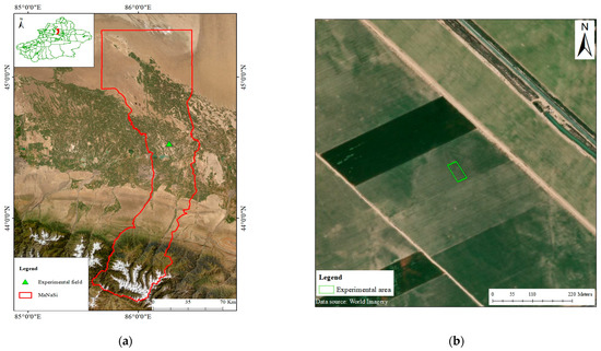
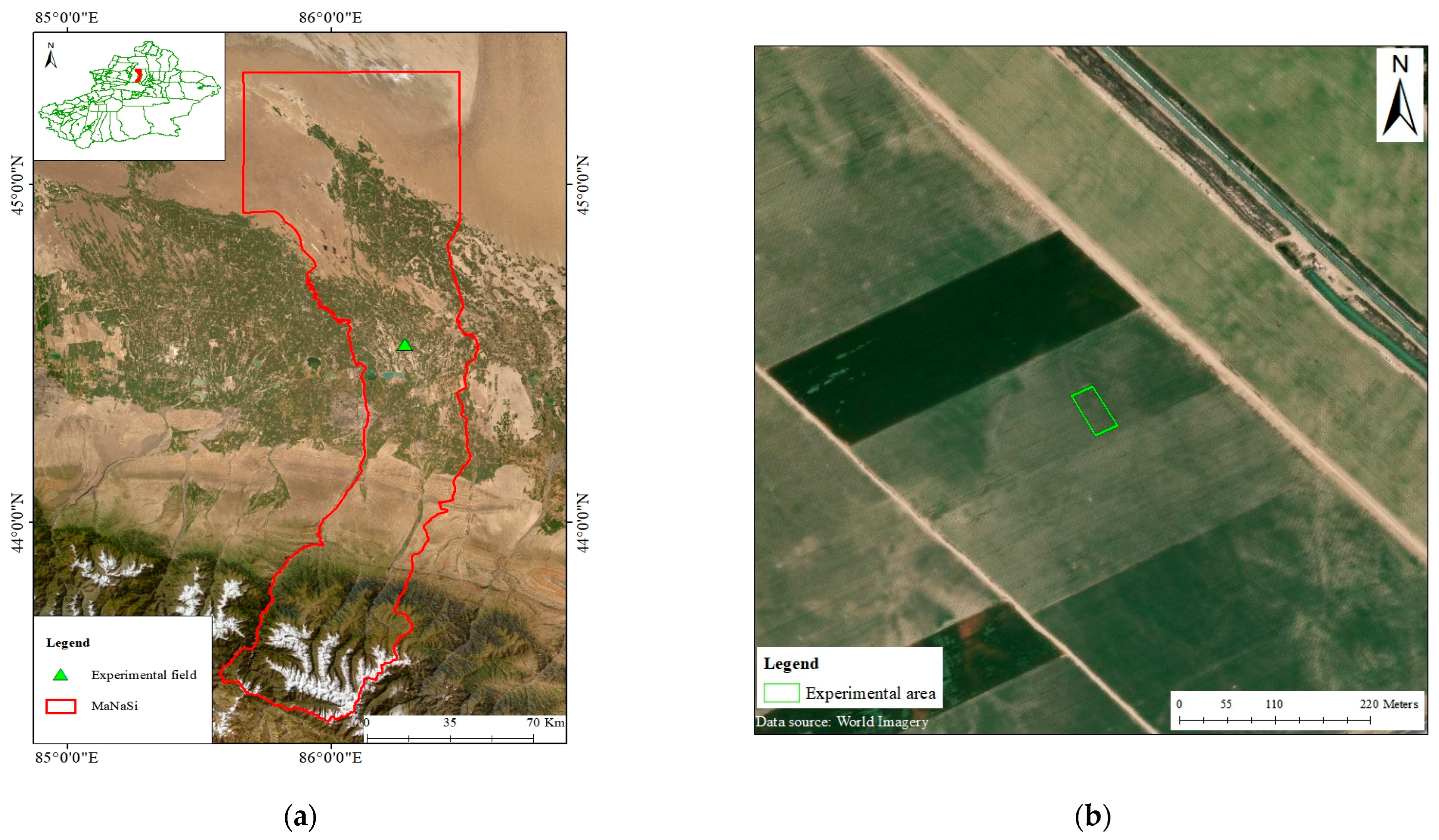
2.1. Experimental Sites

The field experiment was conducted in Manas County, China (86°16′42″ E, 44°31′47″ N), Figure 1. The study area features a typical mid-temperate continental climate, with significant diurnal temperature variations. In 2024, the mean daily maximum air temperature (Tmax) was 15 °C, the mean daily minimum air temperature (Tmin) was 3 °C, and the total precipitation amounted to 232.6 mm. Irrigation was applied using drip irrigation under plastic mulch, with drip tapes laid directly beneath the plastic film and surface-installed at a shallow depth of 1–3 cm below the soil surface; soil preparation followed conventional tillage practices.

Figure 1. Location of the study area and experimental field. (a) The geographical location of Manas County, Xinjiang, China, with the study area outlined in red and the triangle indicating the location of the experimental site. (b) The area within the green line is the field experimental area.

2.2. Experimental Design

In this study, irrigation regime was used as the experimental factor. Four irrigation treatments (0%, 30%, 60%, and 90%) were applied to represent graded water-stress conditions, with three replicates per treatment. Cotton was sown on 15 April 2024 at a sowing density of 2.7 × 10⁵ seeds ha⁻¹. Individual plots measured 25 m in length and 4.5 m in width. Irrigation treatments were initiated 59 days after planting (DAP) in 2024, during which cumulative rainfall totaled 7.03 mm. After treatment initiation, no irrigation was applied in the 0% treatment. The irrigation schedules for all treatments are summarized in Table 1.

Table 1. The irrigation schedule of four treatments at different cotton growth stages in 2024.

Day After Planting (DAP)	0% Irrigation (m3/ha)	30% Irrigation (m3/ha)	60% Irrigation (m3/ha)	90% Irrigation (m3/ha)
6	300	300	300	300
59	0	81	162	243
71	0	82.5	165	247.5
79	0	126	252	378
90	0	123	246	369
97	0	127.5	255	382.5
106	0	124.5	249	373.5
114	0	93	186	279
120	0	90	180	270
127	0	91.5	183	274.5

2.3. Data Acquisition

2.3.1. Field Data Collection

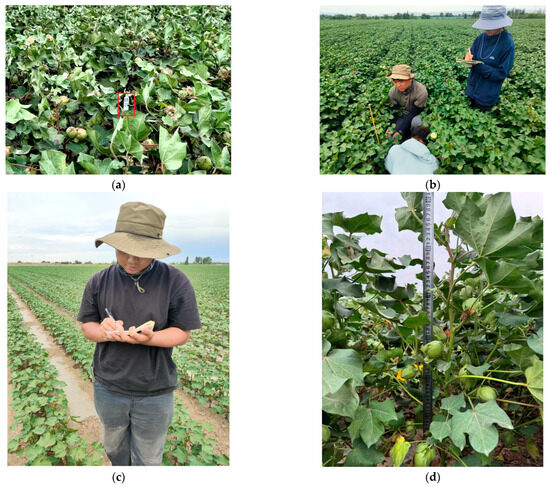
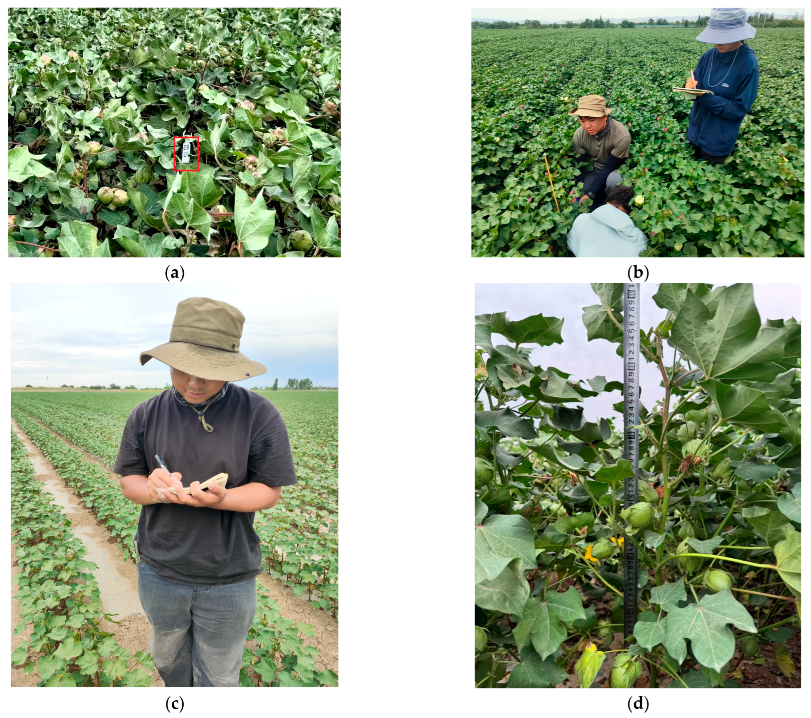
Field data collection was carried out at 41, 71, 112, 138, and 158 days after planting (DAPs) in 2024 (Table 2). In each sampling period, agronomic traits of cotton were measured within 2.25 m × 3 m quadrats, including plant height, flower number, boll number per plant, open boll number, and plant density. Within every quadrat, nine uniform, pest-free plants were randomly selected and tagged with unique barcodes, enabling consistent tracking of the same individuals throughout the growing season (Figure 2). These data were used to evaluate the model’s performance in identifying cotton growth stages under different irrigation treatments.

Table 2. The field data collection under four irrigation treatments at different cotton growth stages in 2024.

Year	UAS Sensor	Day After Planting (DAP)
2024	D-CAM5000	41
		71
		112
		138
		158

Figure 2. The field sampling and plant identification for cotton phenology monitoring. (a) Cotton plant marked with red boxes are used for repeated monitoring of the same individual; (b) field sampling at the boll stage; (c) field sampling at the squaring stage; (d) plant height measurement.

2.3.2. UAS Image Collection and Processing

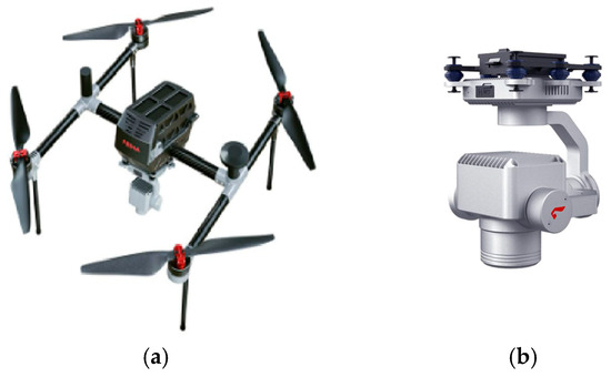
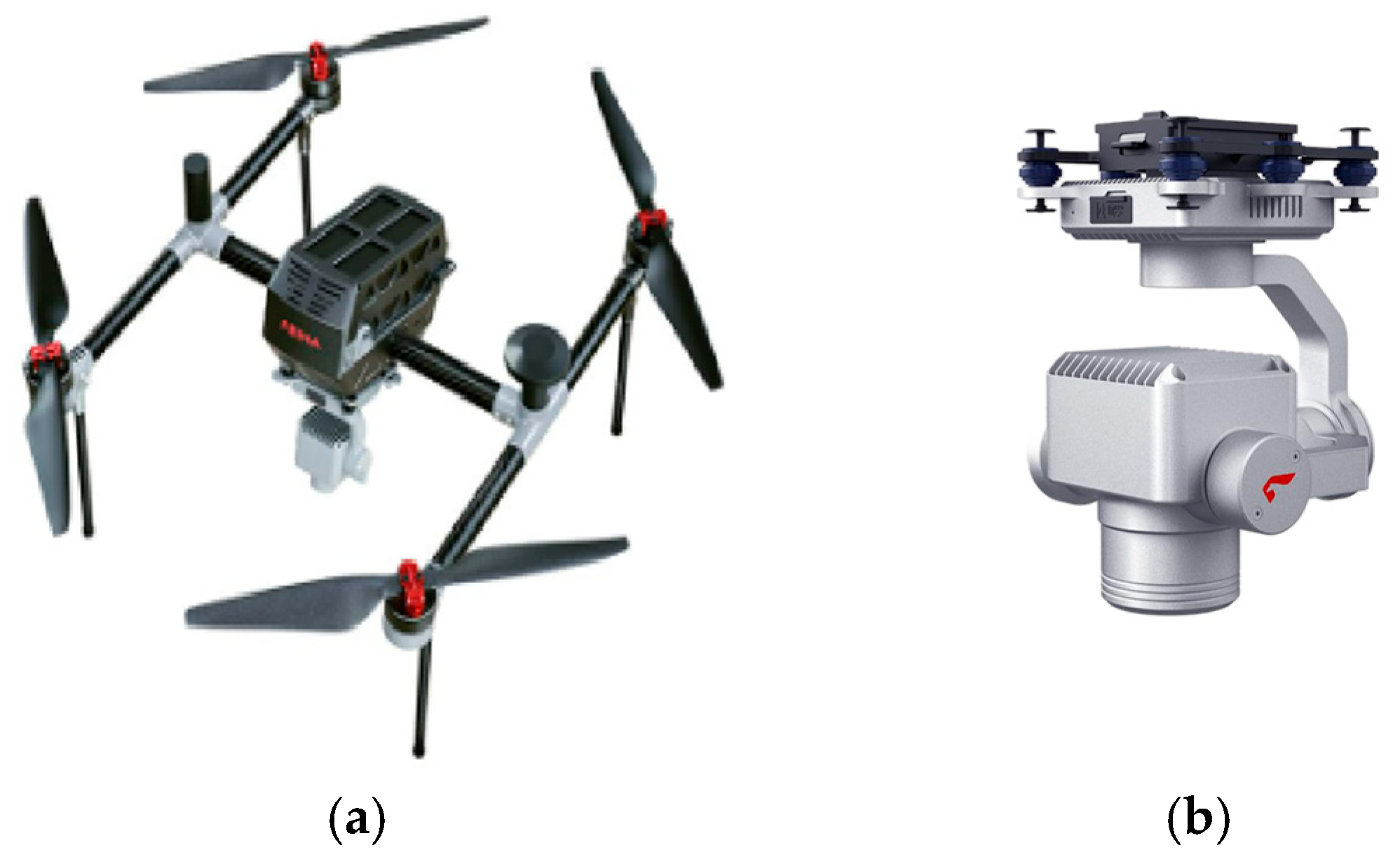
In this study, a D2000S unmanned aerial system (UAS; Feima Robotics, Shenzhen, China) was employed as the aerial platform for high-resolution image acquisition (Figure 3). The UAS was equipped with a D-CAM5000 photogrammetric module (Feima Robotics, Shenzhen, China) integrated with a global-shutter 26-megapixel imaging sensor (6144 × 4096 pixels), with a pixel size of 3.76 μm, an effective sensor size of 23.1 mm × 15.4 mm, and a fixed focal length of 28 mm. UAS data acquisition was synchronized with ground measurements on the same day, with image collection performed prior to the corresponding field observations. Flight plans for image capture were designed and executed using UAVManager software (v1.5.4; Feima Robotics, Shenzhen, China). All flights were conducted at an altitude of 60 m above ground level, with forward and side overlaps both set to 80%, yielding a ground sampling distance (GSD) of 0.8 cm. A total of five flights were carried out from April to October 2024, each corresponding to a key cotton growth stage, as detailed in Table 2. To minimize shadow effects and ensure stable irradiance, image acquisition was performed within approximately two hours around local solar noon (12:00–14:00).

Figure 3. UAS platform and optical (RGB) sensors for visible imaging. (a) Feima Robotics D2000S UAS platform; (b) D-CAM5000 aerial-survey module.

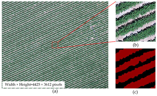
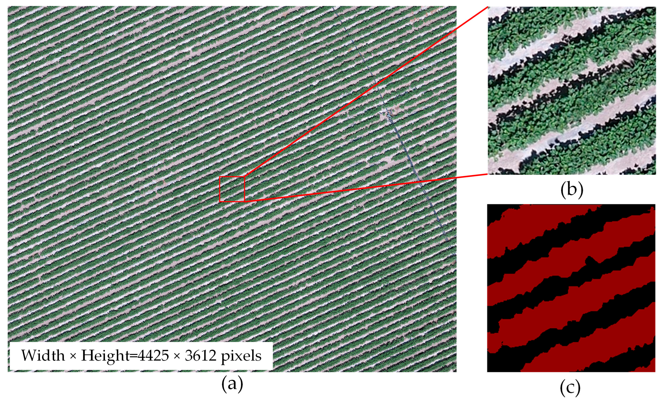
Figure 4a shows the RGB channels of the orthomosaic (partial view) generated from the UAV-acquired imagery. The orthomosaics were processed using the “Smart-Process” and “Smart-Map” modules in UAVManager software (Feima Robotics, Shenzhen, China) to ensure accurate stitching and high image quality. The orthomosaic was then tiled into 256 × 256-pixel image chips using Python (v3.12.6) (Figure 4b). Each image was assigned to one of five semantic classes, including four cotton growth stages (seedling, squaring, boll, and boll-opening) and a background class representing all non-cotton areas. Ground-truth labels were created using the polygon annotation tool in LabelMe and verified by manual visual inspection (Figure 4c).

Figure 4. The UAS image used in this study. (a) The orthomosaic image (partial view); (b) a cropped patch (256 × 256 pixels); (c) the corresponding labeled map for (b).

2.4. Dataset Partitioning

Each single growth-stage dataset contained 2000 images, and the four-stage dataset comprised 8000 images in total. Training and test images were extracted from the surrounding non-treatment large-field area outside the water-stress experimental plots. To reduce spatial autocorrelation and prevent spatial leakage, the large-field dataset was partitioned into non-overlapping spatial blocks (i.e., blocks), and the blocks were then split into training (80%, 1600 images per stage) and testing (20%, 400 images per stage), ensuring that images from the same block were not shared between the two sets. In addition, an external prediction set was reserved from the water-stress treatment plots, including 100 images for each growth stage (400 images in total). These fully unseen images were used exclusively for external prediction and evaluation to assess model generalization under treatment conditions.

2.5. Convolutional Neural Networks (CNN)

In this study, a pixel-level semantic segmentation framework for cotton growth stages was established using three deep learning models (DeepLabv3+, SegNet, and U-Net). The encoder–decoder structure adopted by all the models is appropriate when using high-resolution field-acquired imagery. SegNet decodes by reusing pooling indices in order to conserve spatial topology and lessen computational load [34]. Skip connections are used to incorporate low-level texture and high-level semantic features into U-Net [35]. DeepLabv3+ employs atrous (dilated) convolutions together with an atrous spatial pyramid pooling (ASPP) module in the encoder to capture multi-scale contextual information while keeping the output stride small, rather than further reducing spatial resolution [36,37,38]. Model building was implemented in MATLAB R2023a with the Deep Learning Toolbox (MathWorks, Inc., Natick, MA, USA).

Paired input images and corresponding pixel-level labels were prepared to support cross-growth stage evaluation. To improve robustness and cross-stage generalization, data augmentation was applied on-the-fly (online) to the training set during each epoch rather than via offline preprocessing. Specifically, for each mini-batch, image–label pairs were synchronously transformed using random rotations within −10° to +10° and horizontal flipping [39]. In addition, color jitter was applied to the input images by randomly adjusting brightness and contrast: pixel intensities were multiplied by a factor in the range 0.8–1.2 for brightness, and image contrast was scaled by a factor in the range 0.8–1.2 [40]. Model training was conducted using stochastic gradient descent with momentum (SGDM) with an initial learning rate of 0.01, a mini-batch size of 16, and 50 epochs, with a stepwise learning-rate decay during optimization. These strategies expanded the effective training distribution and enhanced the resilience of the segmentation models.

2.6. Model Accuracy Evaluation

Image-segmentation performance was quantified using Global Accuracy (GA), mean intersection-over-union (mIoU), and mean boundary F1 score (mBF), which collectively capture pixel-level accuracy, boundary alignment, and class balance [41,42,43]:

GA is one of the most fundamental metrics in image segmentation. It measures the overall proportion of correctly classified pixels across all classes and thus offers a direct snapshot of model performance [41]. The metric is calculated as follows:

$$\mathrm{N}={\sum }_{\mathrm{i}=1}^{\mathrm{k}}\left({\mathrm{T}\mathrm{P}}_{\mathrm{i}}+{\mathrm{F}\mathrm{P}}_{\mathrm{i}}+{\mathrm{F}\mathrm{N}}_{\mathrm{i}}\right)$$

(1)

$$\mathrm{G}\mathrm{A}={\displaystyle \frac{{\sum }_{\mathrm{i}=1}^{\mathrm{k}}{\mathrm{T}\mathrm{P}}_{\mathrm{i}}}{\mathrm{N}}}$$

(2)

where N is the total number of pixels in the reference data, TP_i denotes the number of true-positive pixels for class i (pixels that are correctly identified as belonging to class i), FP_i is the number of false-positive pixels for class i (pixels that are incorrectly labeled as class i), FN_i is the number of false-negative pixels for class i (pixels that truly belong to class i but are misclassified as other classes), and k is the total number of classes.

The mBF measures the degree of alignment between the identified object boundaries and the ground-truth boundaries, expressed in the form of an F1-score averaged over all classes [44]. The metric is calculated as follows:

$${\mathrm{P}}_{\mathrm{i}}^{\mathrm{B}}={\displaystyle \frac{{\mathrm{TP}}_{\mathrm{i}}^{\mathrm{B}}}{{\mathrm{TP}}_{\mathrm{i}}^{\mathrm{B}}+{\mathrm{FP}}_{\mathrm{i}}^{\mathrm{B}}}}$$

(3)

$${\mathrm{R}}_{\mathrm{i}}^{\mathrm{B}}={\displaystyle \frac{{\mathrm{TP}}_{\mathrm{i}}^{\mathrm{B}}}{{\mathrm{TP}}_{\mathrm{i}}^{\mathrm{B}}+{\mathrm{FN}}_{\mathrm{i}}^{\mathrm{B}}}}$$

(4)

$${\mathrm{BF}}_{\mathrm{i}}={\displaystyle \frac{2{\mathrm{P}}_{\mathrm{i}}^{\mathrm{B}}{\mathrm{R}}_{\mathrm{i}}^{\mathrm{B}}}{{\mathrm{P}}_{\mathrm{i}}^{\mathrm{B}}+{\mathrm{R}}_{\mathrm{i}}^{\mathrm{B}}+\mathsf{\epsilon }}}$$

(5)

$$\mathrm{mBF}={\displaystyle \frac{1}{\mathrm{C}}}{\sum }_{\mathrm{i}=1}^{\mathrm{C}}{\mathrm{BF}}_{\mathrm{i}}$$

(6)

where TP_i^B denotes the number of correctly identified boundary pixels for class i; FP_i^B and FN_i^B are the numbers of false-positive and false-negative boundary pixels, respectively; ε is a small constant (10⁻⁶) introduced to prevent division by zero; and C represents the total number of classes.

The mIoU quantifies the per-class spatial overlap between identified and reference regions using the intersection-over-union (IoU) and then averages the class-wise IoU scores, yielding a more class-balanced assessment than global pixel accuracy under class imbalance [41]. The metric is calculated as follows:

$$\mathrm{mIOU}={\displaystyle \frac{1}{\mathrm{K}}}{\sum }_{\mathrm{i}=1}^{\mathrm{k}}\left({\displaystyle \frac{{\mathrm{TP}}_{\mathrm{i}}}{{\mathrm{TP}}_{\mathrm{i}}+{\mathrm{FP}}_{\mathrm{i}}{+\mathrm{FN}}_{\mathrm{i}}}}\right)$$

(7)

where TP_i is the number of true-positive pixels for class i, FP_i is the number of false-positive pixels for class i, FN_i is the number of false-negative pixels for class i, and k is the total number of classes.

For all three indices (GA, mIoU, and mBF), values range from 0 to 1, with higher values indicating better overall pixel-wise accuracy, class-averaged region overlap, and boundary localization, respectively [41,45].

2.7. Data Analysis

This study used three evaluation metrics (GA, mIoU, and mBF) to compare three semantic segmentation networks (SegNet, U-Net, and DeepLabv3+) and select the best-performing model. To determine an efficient training sample size, ten repeated experiments were conducted under the optimal model using independent images that were not involved in model development. By progressively increasing the training set size and analyzing performance trends, the sample size that achieved the best and most stable results across repetitions was identified as the optimal training volume. The optimal model and optimal training volume validation were performed using field-measured plots to quantify phenology recognition accuracy and identification consistency across different irrigation treatments under water-stress conditions.

3. Results

3.1. Performance Evaluation of Semantic Segmentation for Individual Cotton Growth Stages

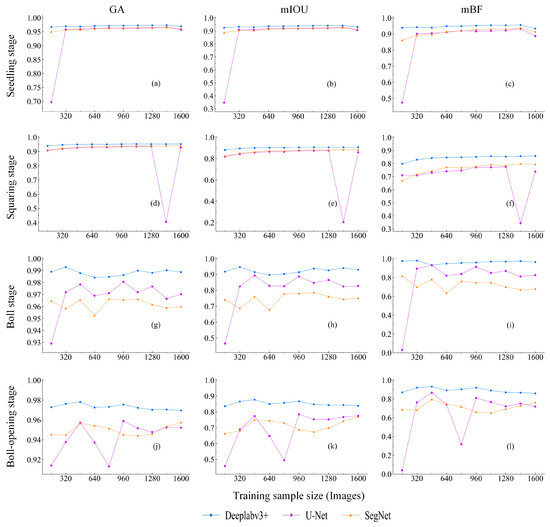
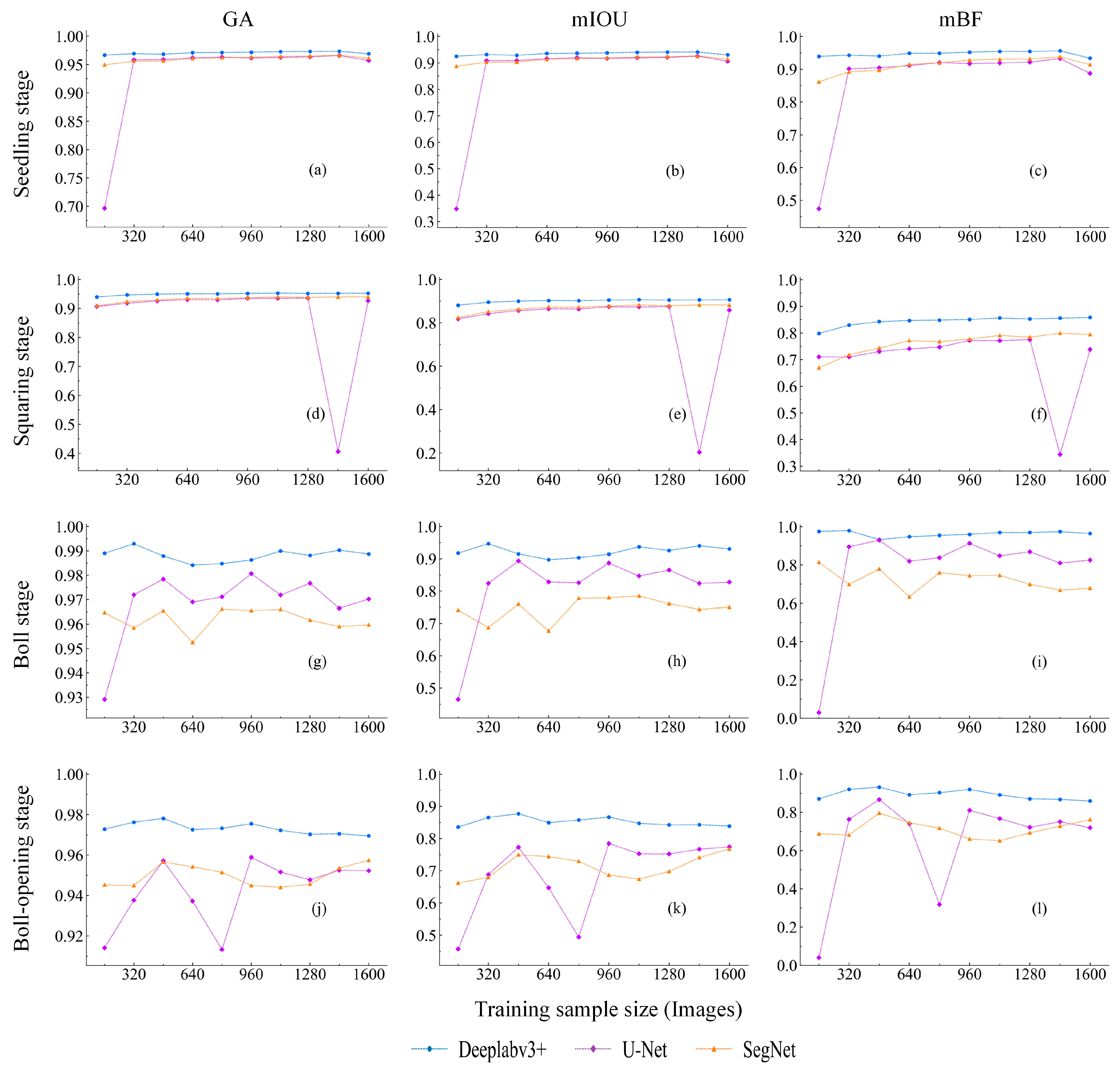
Figure 5 shows the performance evaluation of different algorithms for individual cotton growth stages. At the seedling phase (Figure 5a), DeepLabv3+ demonstrated the highest level of segmentation performance when it was trained on 1440 images, and its mIoU was 0.94, GA was 0.97, and mBF was 0.96. Although SegNet and U-Net achieved GA results similar to DeepLabv3+ with a training sample size of 800 images, their mIoU and mBF rates were always lower than those of DeepLabv3+. The peak performance of DeepLabv3+ was achieved at a training sample size of 1120 images in the squaring stage, where the respective measures of mIoU, GA and mBF were 0.91, 0.95 and 0.86 (Figure 5b). Even though SegNet and U-Net had a close approximation of DeepLabv3+ GA at 960 training images, their continual inability to perform as well in terms of mIoU and mBF points to their low effectiveness in the task of representing growth stage features and boundaries of target regions.

Figure 5. The accuracy evaluation of three deep learning models (DeepLabv3+, U-Net, and SegNet) using three evaluation metrics (GA, mIoU, and mBF) under different training sample sizes for each individual cotton growth stage in 2024.

During the boll stage (Figure 5c), DeepLabv3+ showed the best segmentation results even with a fairly small training sample of 320 images, with a result of mIoU of 0.95, GA of 0.99, and mBF of 0.98. Conversely, although SegNet and U-Net produce similar GA values, their much smaller mIoU and mBF scores signify that they are less effective in separating bolls from the background environment. At the boll-opening stage (Figure 5d), DeepLabv3+ reached its peak performance, which was at 480 training images, with measurements of mIoU = 0.88, GA = 0.98 and mBF = 0.93. At this same sample size, in which SegNet and U-Net once again demonstrated GA equal to DeepLabv3+, their mIoU and mBF scores were still significantly low across all experiment settings.

Figure 6 shows how DeepLabv3+ has qualitative gains over SegNet and U-Net on a per-stage basis. As shown in Figure 6a, DeepLabv3+ successfully identified inter-row weeds as weeds and cotton seedlings as seedlings, whereas SegNet and U-Net had low separability with frequent mislabeling of weeds as seedlings. In Figure 6b, DeepLabv3+ is highly reliable in determining sparsely spaced cotton plants at the squaring stage, but SegNet and U-Net tend to miss individual specimens, leading to incomplete segmentation masks. DeepLabv3+ in Figure 6c was able to distinctly separate the bare soil and cotton canopy, whereas SegNet and U-Net misidentified part of the soil as cotton and almost all the soil was misidentified as a target object, respectively. In Figure 6d, DeepLabv3+ offered a more precise distinction between cotton and weeds when the cotton reached the stage of opening the bolls. The SegNet was able to partially define weed patches, but its boundaries were not as accurately defined, and the U-Net did not detect most of the weeds. All these observations support the fact that DeepLabv3+ always outperforms SegNet and U-Net in all four stages of cotton growth.

Figure 6. Representative cotton segmentation results on the test set for different deep learning models and training sample sizes at four growth stages. (a) Seedling stage; (b) squaring stage; (c) boll stage; (d) boll-opening stage.

3.2. Performance Evaluation of Deep Learning Models in Cotton Growth Stages Identification

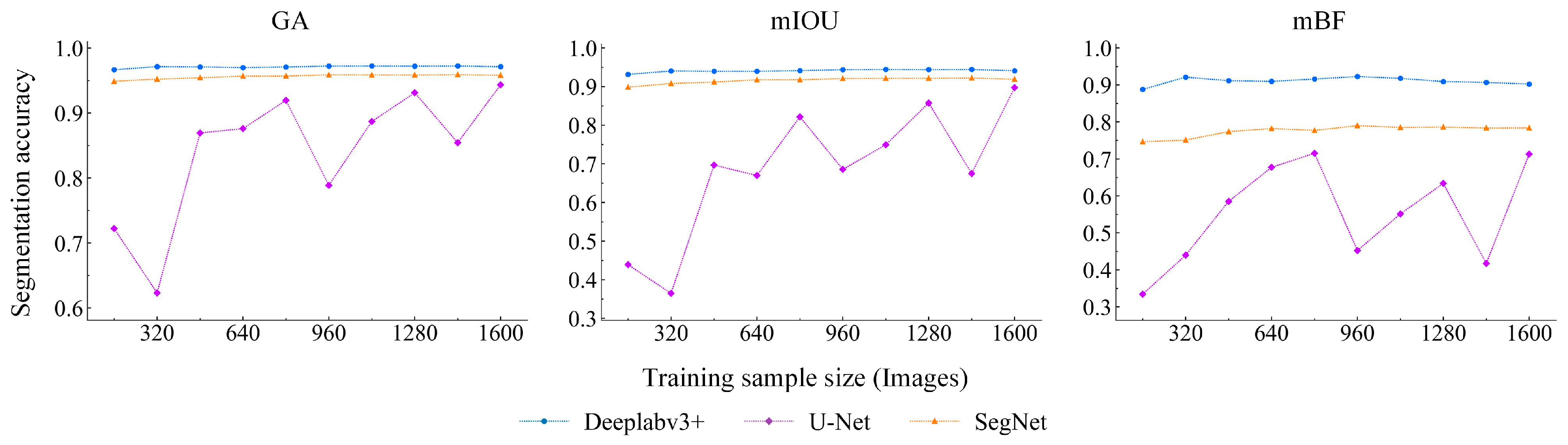
For the full-season dataset (Figure 7), DeepLabv3+ exhibited the most robust segmentation performance among the three models, with its mIoU ranging from 0.94 to 0.95, GA from 0.97 to 0.98, and mBF from 0.90 to 0.94. In the case of SegNet, the GA at a training size of 960 images (0.96) was close to that of DeepLabv3+ (0.98), suggesting that the discrepancy in overall pixel-level accuracy was relatively marginal at this training scale. Nevertheless, SegNet’s mIoU and mBF remained at a comparatively lower range of 0.90–0.92 and 0.75–0.79, respectively. In particular, reduced mBF values showed that SegNet was worse than DeepLabv3+ at capturing class-specific spatial overlaps and fine-grained details related to boundaries.

Figure 7. The accuracy evaluation of three deep learning models (DeepLabv3+, U-Net, and SegNet) using three evaluation metrics (GA, mIoU, and mBF) to compare the performance of cotton segmentation models throughout the season.

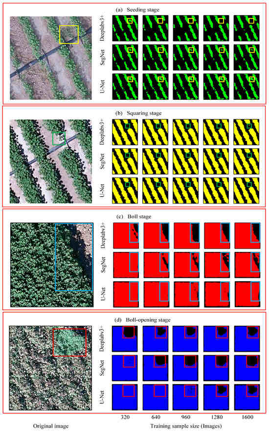
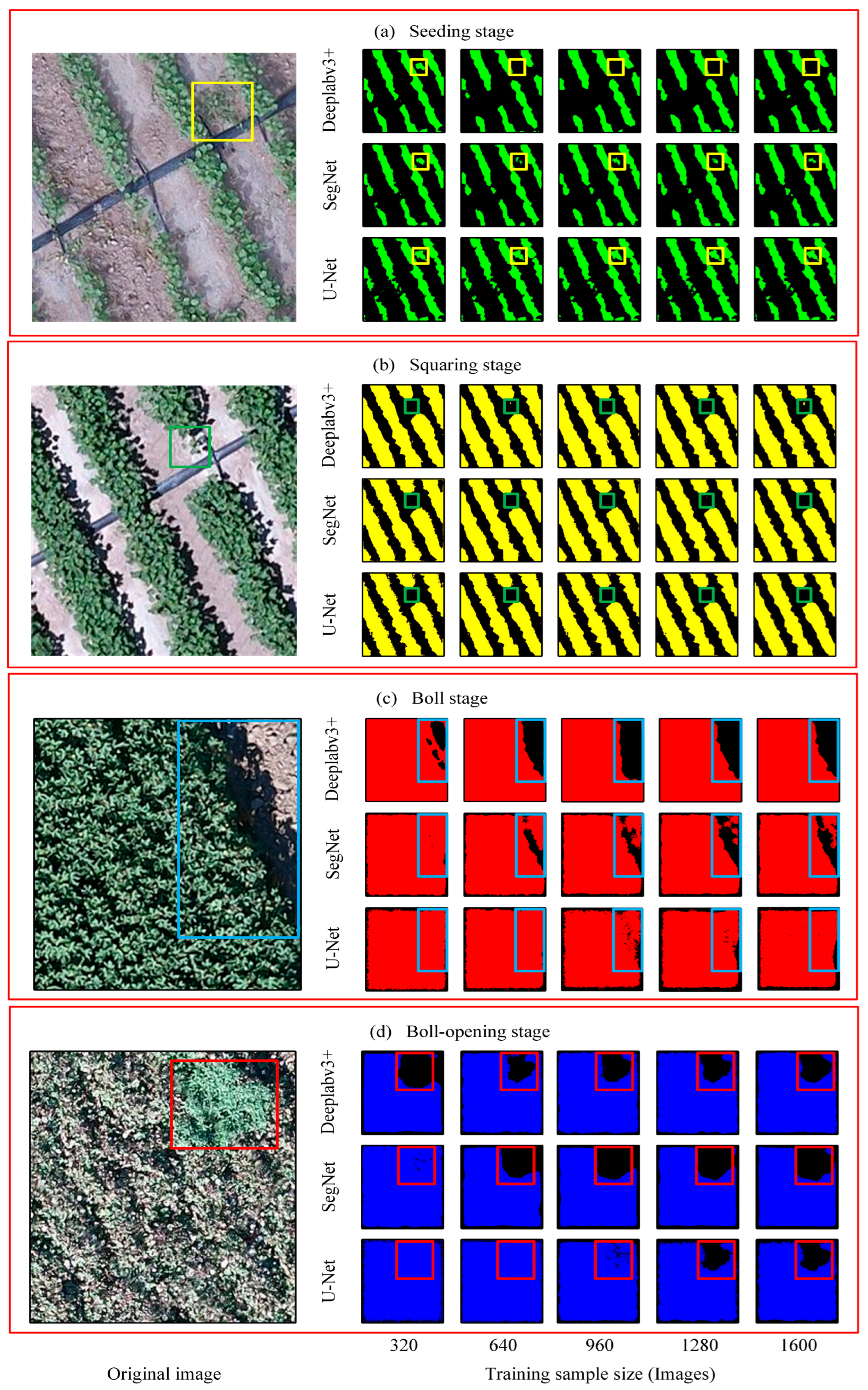
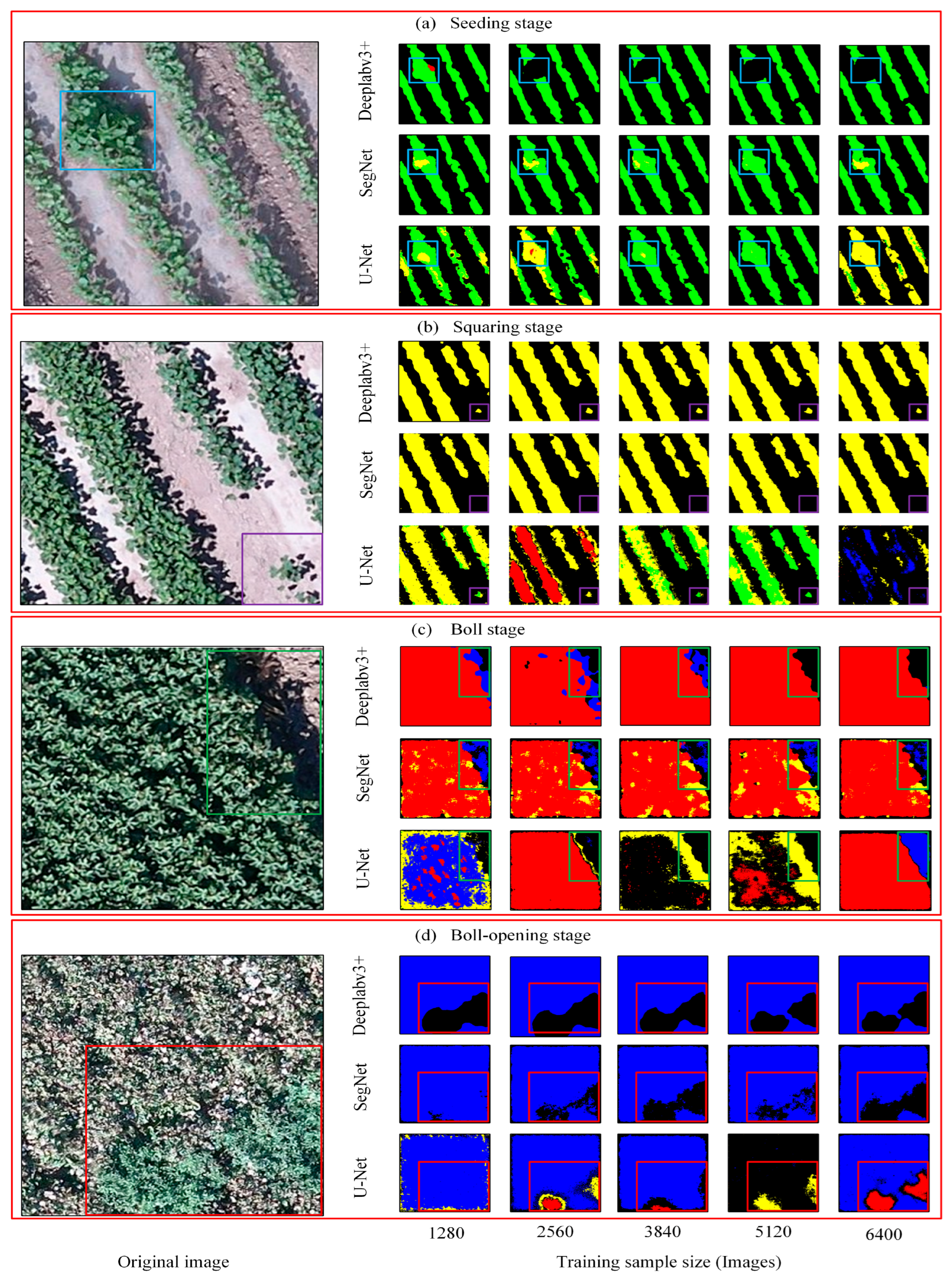
The outcomes of the visual segmentation also confirmed the indicated trends (Figure 8). At the seedling stage, DeepLabv3+ successfully maintained the structural thinness of small seedlings with more distinct and continuous contour boundaries and hence reduced fragmented omission mistakes. Conversely, SegNet and U-Net were more susceptible to incorrectly identifying weeds or areas that had similar textures as cotton, which led to increased levels of false positives and ambiguous border definition (Figure 8a). In the squaring stage, DeepLabv3+ was still able to extract sparsely distributed plants in nearly complete form. SegNet tended to miss weak isolated targets, and U-Net failed due to local category confusion and unsteady boundary segmentation (Figure 8b). During the boll and boll-opening stages, the increased background heterogeneity coupled with intensified illumination and shadow effects exacerbated the segmentation errors of SegNet and U-Net (Figure 8c,d). Overall, DeepLabv3+ maintained superior boundary adherence and target shape consistency across all growth stages, demonstrating enhanced segmentation robustness.

Figure 8. Representative cotton segmentation results on the test set for different deep learning models and training sample sizes across the full growing season. Panels (a–d) correspond to the seedling stage, squaring stage, boll stage, and boll-opening stage, respectively.

3.3. Effects of Sample Proportion on Classification Accuracy

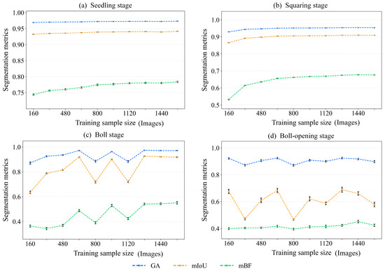
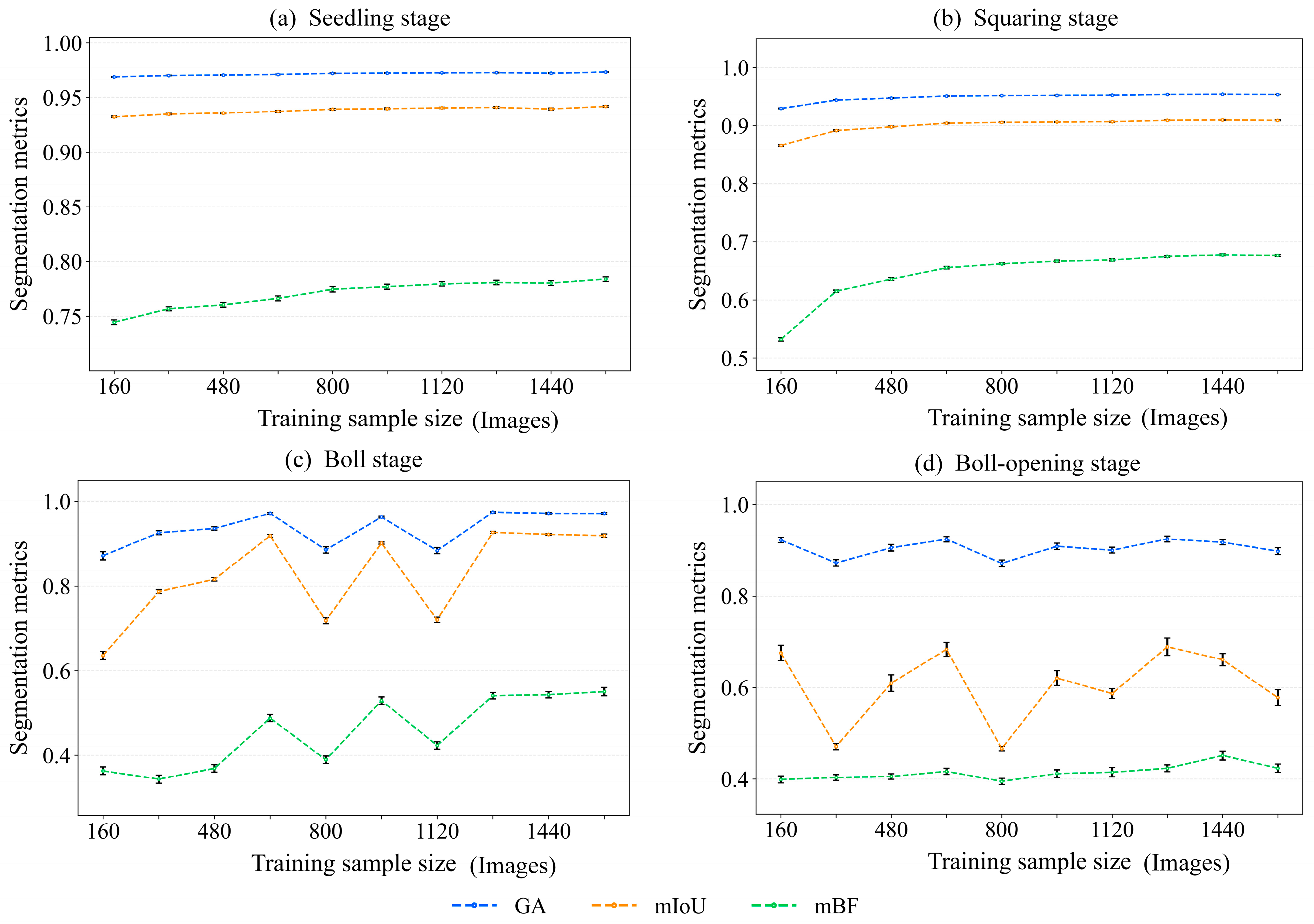
During the seedling stage (Figure 9a), the GA remained stable at 0.97 across the training sample size range from 160 to 1600 images. In contrast, the mean mIoU increased marginally from 0.93 to 0.94, while the mean mBF exhibited a stepwise upward trend, increasing from 0.74 with 160 samples to 0.77 with 800 samples and reaching its peak and stabilizing at 0.78 when the sample size was 960 or higher.

Figure 9. Semantic segmentation performance of DeepLabv3+ under different training sample sizes across cotton growth stages. Results are reported as the mean (±standard deviation) of three evaluation metrics (GA, mIoU, and mBF) over 10 repeated runs. (a) Seedling stage; (b) squaring stage; (c) boll stage; (d) boll-opening stage.

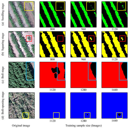
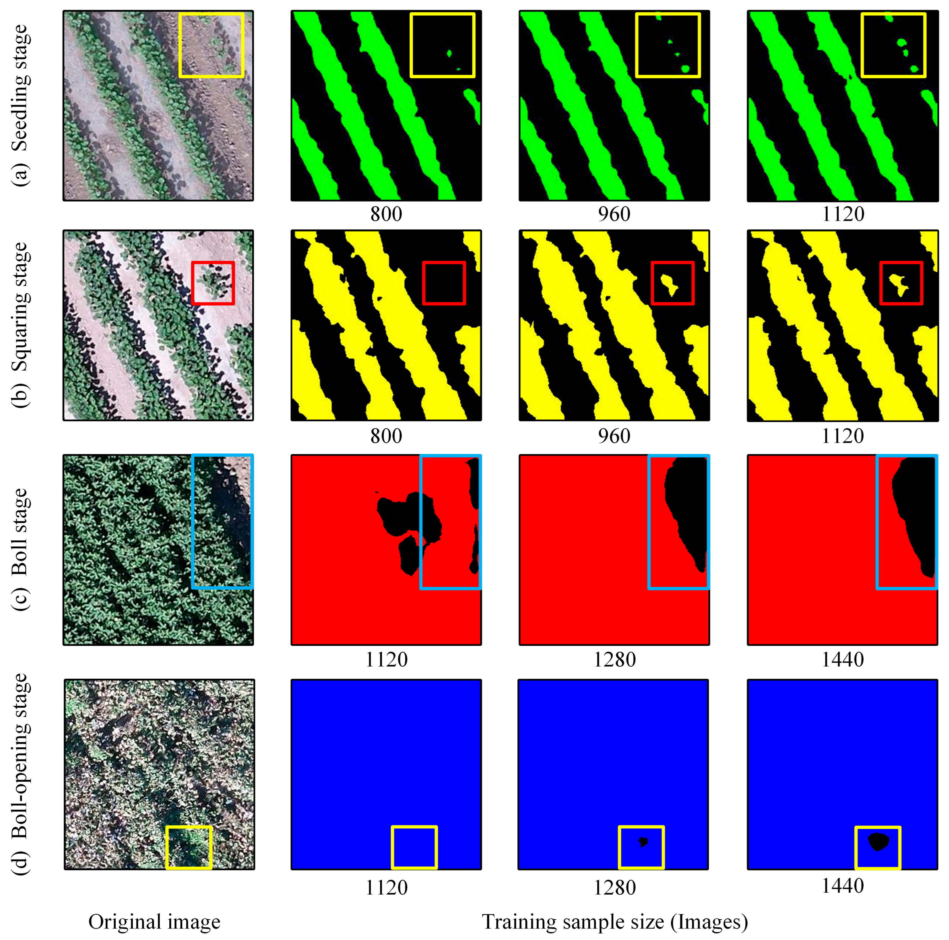
For the squaring stage (Figure 9b), GA increased from 0.93 (160 samples) to 0.95 (640 samples) and plateaued at this level thereafter. Meanwhile, mIoU climbed from 0.87 (160 samples) to 0.90 (640 samples) and stabilized at 0.91 when the sample size exceeded 800. The mBF metric entered a stable phase within the 960–1600 sample range, with values fluctuating slightly within the narrow interval of 0.67–0.68. These quantitative trends were consistent with the observations derived from qualitative segmentation maps. As the sample size of the training increased to 960, it can be seen in Figure 10a that the omission and misclassification of small seedling targets decreased significantly, and in Figure 10b, the division boundaries of target areas started to look more distinct.

Figure 10. Representative DeepLabv3+ cotton segmentation results on the independent external prediction dataset at the optimal training sample size for each growth stage. (a) Seedling stage; (b) squaring stage; (c) boll stage; (d) boll-opening stage.

In the boll stage (Figure 9c), the GA showed a clear wavering pattern as the size of the training sample grew: it started at 0.87 at 160 samples, went up to 0.97 at 640 samples and down to 0.89 and 0.88 at 800 and 1120 samples and finally bounced back to steady at 0.97 between 1280 and 1600 samples. The trend in mIoU remained constant: the value increased between 0.64 (160 samples) and 0.92 (640 samples) and decreased to 0.72 during the 800–1120 sample range before stabilizing at 0.92–0.93 with more than 1280 samples. In contrast, the average mBF was 0.36 (160 samples) and rose to 0.49 (640 samples) and leveled off at 0.54–0.55 with the larger sample sizes of 1280 and higher.

As shown in Figure 9d, during the boll-opening process, GA oscillated slightly over a small interval of 0.87–0.92, and had local minimum values of 0.87 at 320 and 800 samples with values of 0.90–0.92 between 960 and 1600 samples. In comparison, mIoU showed wide variation: it had a minimum of 0.47 at both 320 and 800 samples, peaked at 1280 samples (0.69) and then fell marginally to 0.58 at 1600 samples. The metric of Mbf grew steadily up to 0.40 (160 samples), 0.41 (1120 samples), stayed in the range of 0.42–0.45 with 1280–1600 samples, and finally reached its highest point of 0.45 with 1440 samples.

Figure 10 shows that under the condition of inadequate training samples, segmentation errors became more obvious. In the seedling and squaring (Figure 10a,b) stages, with a limited training sample size of 800, the model could not reach a steady plant detection in dispersed situations, which was achieved at a sample size of 960. In the boll and boll-opening (Figure 9c,d) stages, small sample sizes were also associated with significant misclassification errors and lack of continuous segmentation boundaries; those problems were significantly reduced when the sample size was extended to 1280, producing more consistent segmentation masks with better boundary continuity and finer detail preservation. On average, DeepLabv3+ showed higher boundary characterization capacity and cross-growth-stage detection uniformity.

3.4. Training Sample Size Requirement for Cross-Phenological-Stage Cotton Segmentation

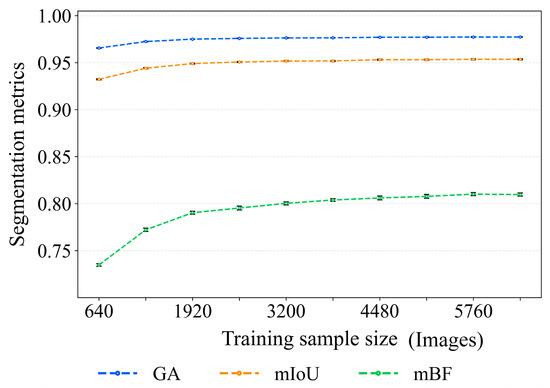
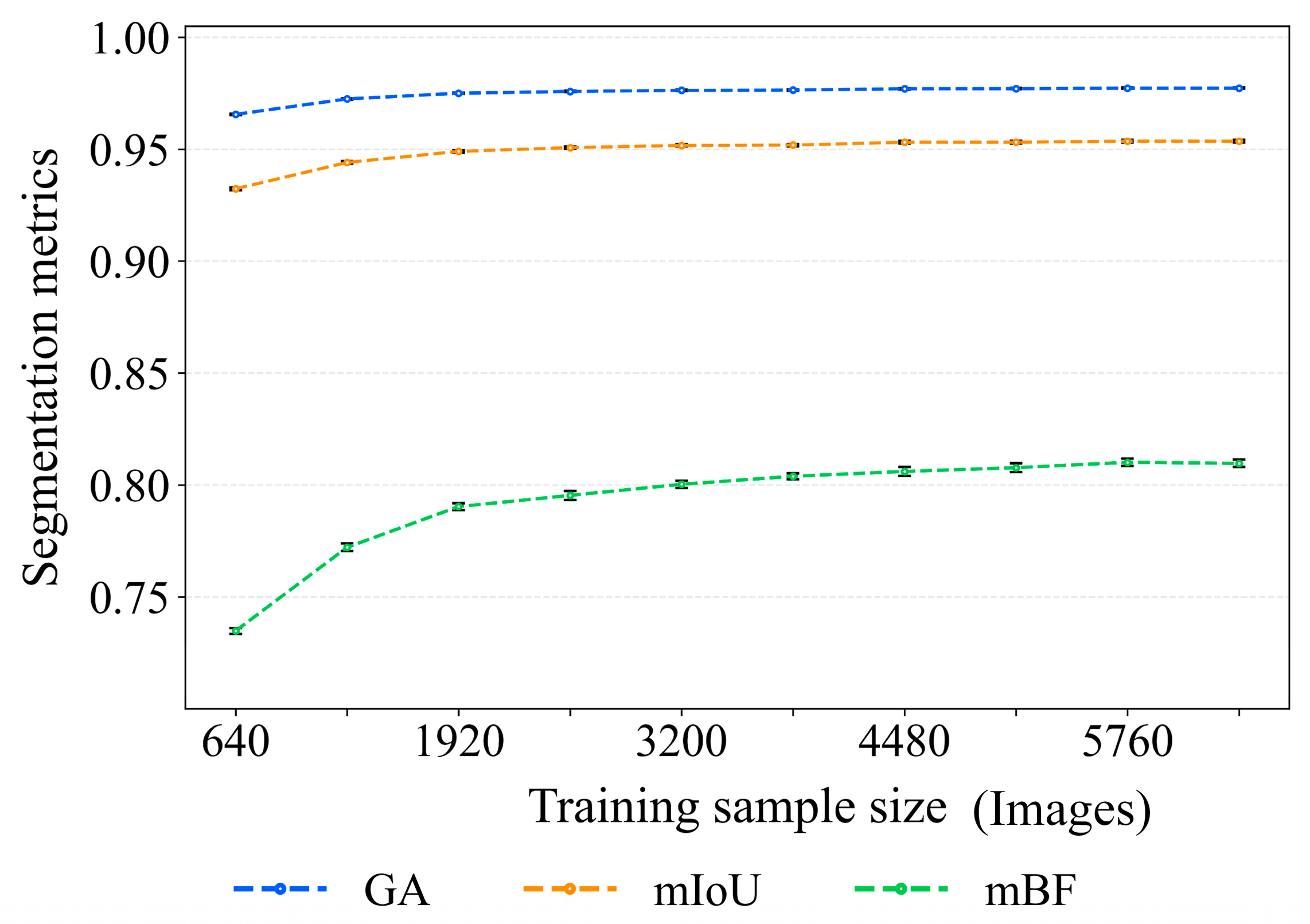
To quantify the training data demand for cross-phenological-stage segmentation (i.e., without stratifying the segmentation task by growth stages), full-season experiments were implemented under consistent training configurations, where training subsets with sample sizes ranging from 640 to 6400 at an interval of 640 were adopted. As illustrated in Figure 11, the GA and mIoU exhibited the most substantial increments within the sample size range of 640–1920, followed by a gradual deceleration in the rate of performance improvement. Once the training sample size reached 4480, both metrics essentially stabilized at 0.98 for GA and 0.95 for mIoU, respectively. In contrast, the mean boundary F1-score (Mbf) demonstrated a stronger dependence on sample size. It increased steadily from 0.74 to 0.81 as the sample size expanded, with only marginal fluctuations observed in the 4480–6400 sample interval.

Figure 11. Effect of training sample size on full-season cotton segmentation performance using DeepLabv3+. Results are reported as the mean (±standard deviation) of three evaluation metrics (GA, mIoU, and Mbf) over 10 repeated experiments.

3.5. Phenology Identification Consistency Across Irrigation Treatments

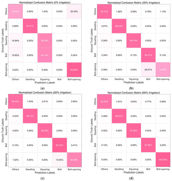
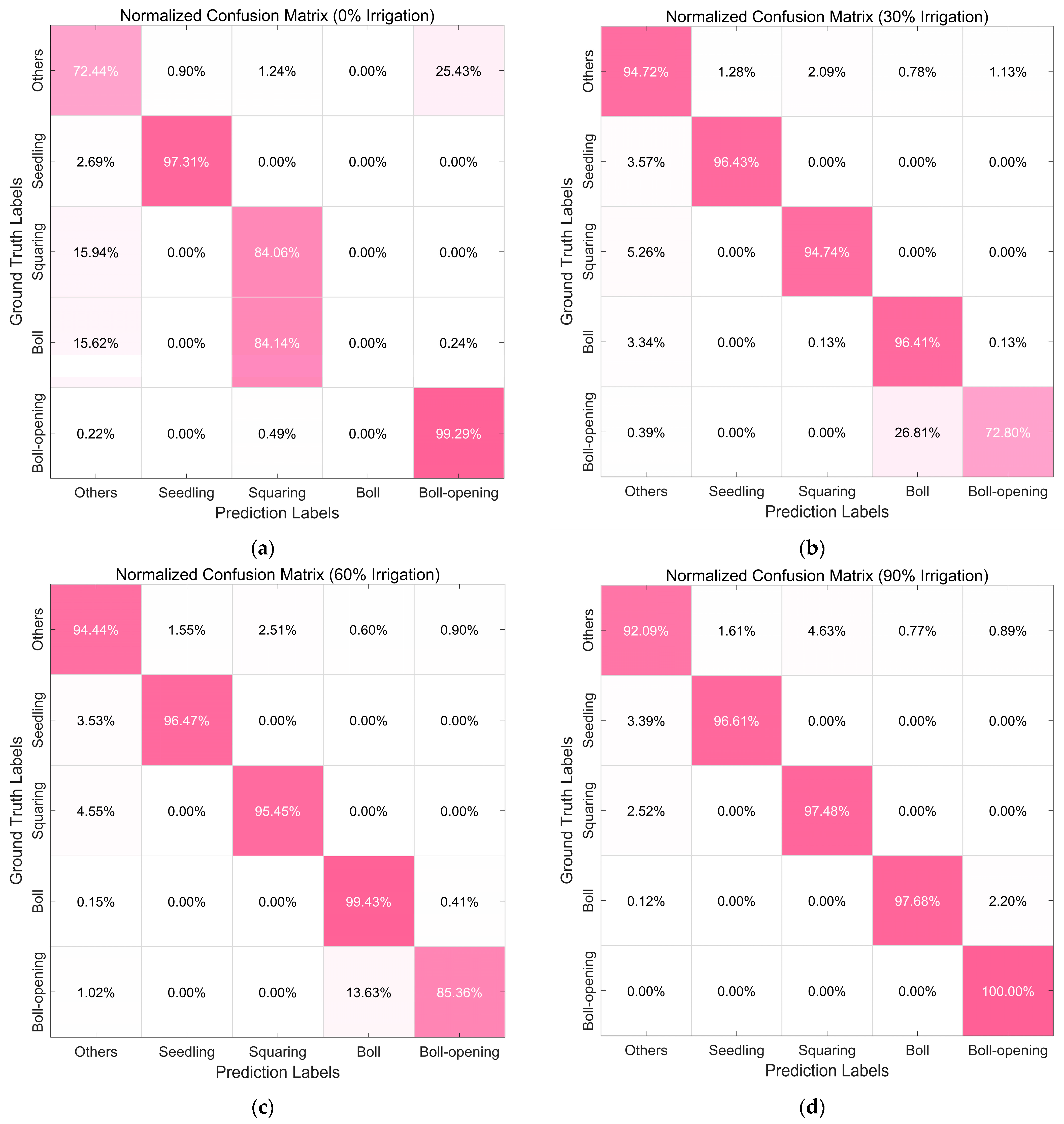
Under the 0% irrigation treatment (Figure 12a), the model performed well in identifying the seedling (97.31%) and boll-opening (99.29%) stages, with 84.14% of the boll stage identified as squaring stage and 15.62% identified as other stages. In addition, a notable confusion was observed between others and boll-opening, with 25.43% of others identified as boll-opening, and 15.96% of squaring was misclassified as others. At 30% irrigation (Figure 12b), the seedling, squaring, and boll stages showed a certain level of mislabeling as “others” with an error rate of approximately 3–5%, while boll-opening was predominantly confused with boll (26.81%). With 60% irrigation applied (Figure 12c), a similar “others” confusion (3–5%) persisted for the seedling and squaring stages, and boll-opening remained mainly misclassified as boll (13.63%). In the 90% irrigation regime (Figure 12d), the misclassification of seedling and squaring stages as “others” further decreased to approximately 2–4%; additionally, the boll stage was misclassified as boll-opening (2.20%), whereas boll-opening achieved 100% correct classification.

Figure 12. Row-normalized pixel-level confusion matrices for multi-class cotton phenology classification under four irrigation treatments, evaluated on an independent external prediction dataset and generated by the DeepLabv3+ model trained with the optimal sample size. Rows denote ground-truth classes and columns denote identified classes. Diagonal entries indicate the correctly classified proportion (i.e., recall) for each class. (a) 0% irrigation treatment, (b) 30% irrigation treatment, (c) 60% irrigation treatment, and (d) 90% irrigation treatment. Note: The darker the color, the higher the recognition accuracy.

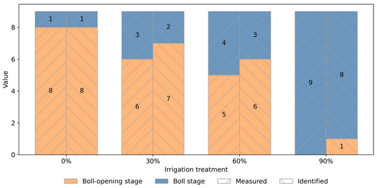
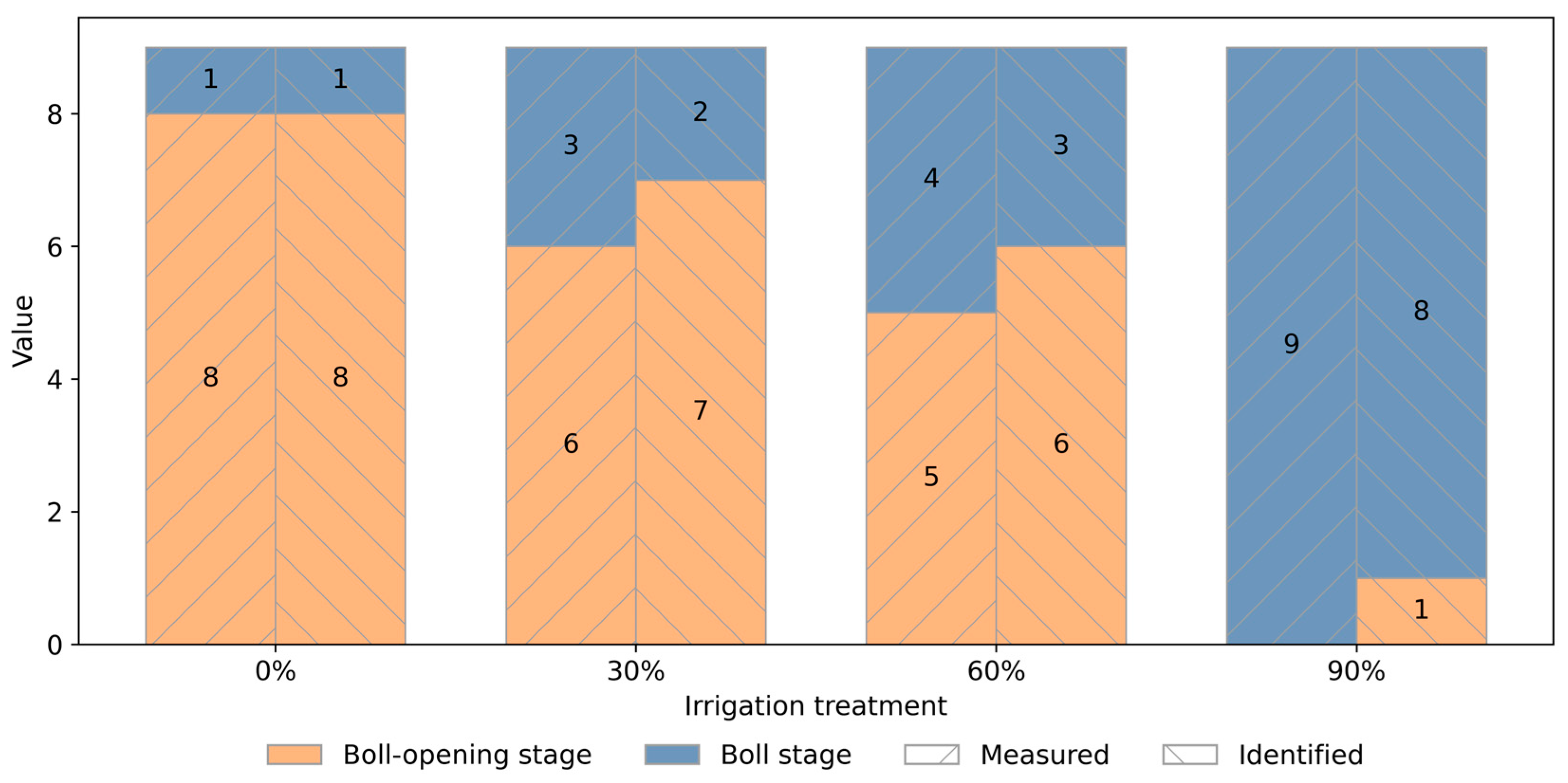
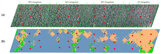
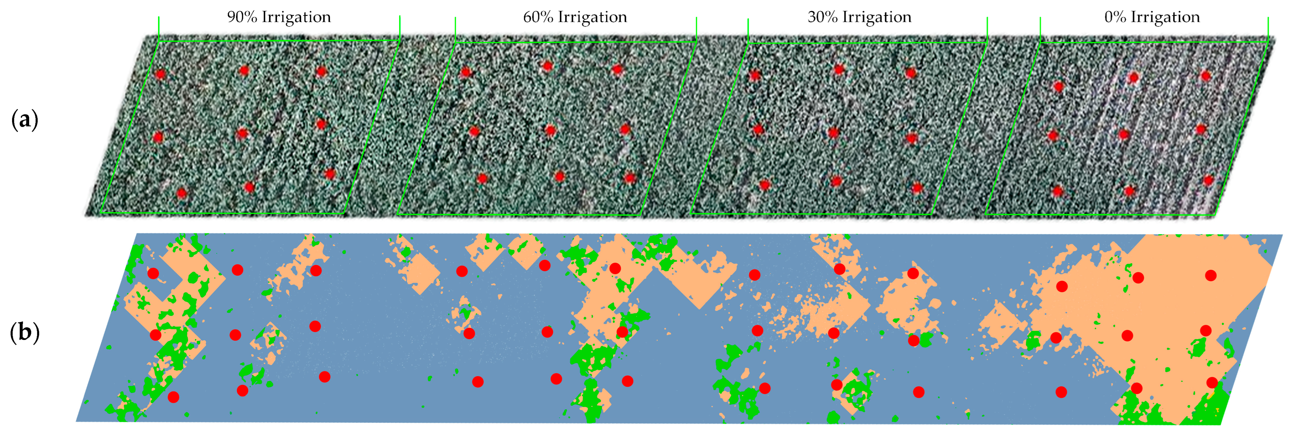
At DAP 138, field observations from 36 in situ sampling points (9 samples per irrigation treatment) indicated a pronounced irrigation-gradient effect on cotton phenology (Figure 13). Under the 0% irrigation treatment, only one sample remained in the boll stage, while the others were in the boll-opening stage. In contrast, under the 90% irrigation treatment, all samples were classified as the boll stage. At the 30% and 60% irrigation levels, as irrigation decreased, the sample distribution progressively shifted toward the boll-opening stage. Overall, the model identification results reproduced the same trend (Figure 14).

Figure 13. Comparison between field-measured cotton phenology and the model identification at DAP 138 under four irrigation treatments (0%, 30%, 60%, and 90%). For each treatment, the grouped stacked bars show the number of samples assigned to the boll stage and boll-opening stage, with measured and identified results distinguished by different fill patterns.

Figure 14. Original UAS image and cotton growth stage identification results using DeepLabv3+ at DAP 138. The 36 red dots in both panels indicate the in situ sampling locations. (a) Original UAS images of the experimental plots under the 0%, 30%, 60%, and 90% irrigation treatments. (b) Identified cotton phenology map using the DeepLabv3+ model; green indicates the “other” class, blue-gray indicates the boll stage, and orange indicates the boll-opening stage.

4. Discussion

In this study, DeepLabv3+ consistently achieved the most robust and stable segmentation performance, in agreement with agricultural remote sensing studies reporting the advantage of DeepLab-family architectures for crop mapping [46,47,48]. The reason behind this superiority is the multi-scale contextual aggregation mechanism of the model due to the use of ASPP encoders and explicit decoder architectures that preserve the fine-grained spatial information and enhance the boundary separation in complicated field conditions [49,50,51]. This overall accuracy level is also equivalent to the average IoU (~0.91) given by UAV-based phenology-stage mapping studies involving deep learning, which serves as the external standard to judge the high performance recorded in this study [30]. Conversely, SegNet and U-Net were less capable of resolving spatial overlaps between classes and maintaining more delicate boundary cues [51,52,53]. At the seedling stage, such models were more often mistaken for inter-row weeds and cotton seedlings, with strong background false positive results; at the squaring stage, they were more prone to miss isolated plants, leaving the detection incomplete. Their boundaries also became less stable during the boll and boll-opening stages, and this was shown as over/under expansion of the target areas, jagged edges, and sometimes local fusion. In addition, the reflective mulch, bright soil patches and shadow margins were more easily misclassified as objects of interest, blurring the target–background interface and lowering boundary-sensitive scores (e.g., mBF) [54,55,56].

The stage-specific quantitative analyses show that the boll and boll-opening stages have a relatively poor segmentation performance and both are limited by the structural complexity of the cotton canopies and severe background interference. In particular, canopy closure and self-shadowing increase intra-class radiometric variation, whereas mixed backgrounds (e.g., soil, plastic-film reflections, and shadow boundaries) decrease separability between classes. Errors in segmentation are found on important morphological interfaces (e.g., canopy margins and open-boll edges), where small delineation errors compromise the uniformity of cotton row configurations and cause non-continuous segmentation borders [57,58]. Such interface-focused errors tend to disproportionately compromise boundary-sensitive measures (e.g., mBF), and such effects are probably exacerbated in subsequent developmental stages when boundary conditions are further spatially heterogeneous. Contextual modeling at multiple scales (e.g., ASPP with explicit decoder) can help stabilize boundary identification in cluttered environments [59].

The increase in the training sample size enhanced segmentation performance. Nonetheless, once the performance reached a plateau, the representativeness of the training dataset was more important than adding further samples [60]. This tendency was evident in our stage-related experimental findings: the boll and boll-opening stages required more diverse image patches in training datasets to provide a stable and precise boundary delineation compared to the seedling and squaring stages. Such differences were mainly due to the increased intra-class heterogeneity and inter-class similarity in such later development stages, caused by the intricate nature of canopy structure (e.g., closure of canopy and gaps between canopies), changing light conditions (e.g., shadows), and reflective components of the background [61]. Training sets that were inclusive of all major variability sources, such as illumination/shadow disparities, soil/plastic-film background, different canopy structural states, and varying row-appearance changes, were much more likely to produce strong and transferable decision rules in the segmentation model, and thus, be successful in preventing segmentation results fragmentation, unlike datasets that consisted of repetitive and homogenous field scenes [62]. A practical construction of a data workflow to balance model generalization capacity and annotation expense would be to first create a representative core training set, then expand the specific datasets through strategic image acquisition and pixel-level labeling. The extension should be made to the less-sampled growth stages, non-typical imaging conditions and hard-segmentation cases (e.g., stage-transition areas, shadow-dominated areas, and cluttered field backgrounds) [63,64]. Also, the introduction of uniform labeling procedures is imperative to ensure the objective assessment of the quality of segmentation boundaries in the boll and boll-opening stages because small differences in labeling practices at important interfaces (e.g., canopy margins and opened-boll margins) may introduce large errors in the evaluation measures based on boundaries [65,66].

Remarkably, the model showed good results in growth stage classification despite drought stress conditions that sped up the phenological development of crops. This observation indicates that the segmentation model primarily relied on phenology-relevant structural cues, which remain stable under water-deficit stress, rather than radiometric appearance traits that are sensitive to environmental stressors [67,68,69]. Previous UAS-based crop monitoring studies have demonstrated that the dynamics of crop water status and pre-visual canopy morphological changes can facilitate the accurate interpretation of growth stages [69]. However, drought stress can introduce domain shift at inference time by altering both canopy structure and background appearance, such as reduced canopy density, decreased leaf area, more canopy gaps with greater soil exposure, and altered shadow distribution patterns, thereby degrading model generalization [70]. Importantly, our use of an independent, fully unseen prediction set from the treatment plots provides a practical test of cross-treatment generalization, which is essential for operational deployment in heterogeneous irrigation scenarios. Thus, for practical deployment scenarios, model evaluation should explicitly quantify cross-treatment generalization capability, for example, by adopting cross-validation schemes in which models are trained under normal irrigation conditions and tested under drought stress [71,72,73]. This assessment structure also highlighted the significance of developing training datasets across various levels of water irrigation (such as 0, 30, 60 and 90 percent) and incorporating the periods of phenological transitions instead of depending mainly on well-watered samples to train models [74,75]. Our situation was such that there were insufficient and unequally distributed labeled data during drought-stress treatments and transition phases, restricting the construction of a dense, continuous drought-gradient training set, which will be considered in future data collection. In addition, the combination of the red-edge and thermal sensing modes is an effective extension to improve the water stress sensitivity of the model [76,77]. Namely, the red-edge spectral indices are highly associated with the amount of chlorophyll and the physiological behavior of vegetation, and the thermal measurements indicate the dynamics of canopy temperatures related to the plant transpiration [78]. Such a multi-sensor remote sensing data fusion approach is likely to be very useful in enhancing the discrimination of crop growth stages where the contrast in RGB imagery is low [79,80].

In the present study, we proposed a UAS-based framework to identify cotton phenological states at various levels of irrigation. The proposed UAS–DeepLabv3+ workflow enabled cost-effective, field-scale phenology mapping under irrigation gradients [81,82]. It provided actionable growth-stage information for precision crop management in arid cotton-growing regions, supporting zone-based irrigation scheduling and drought-responsive field operations [83]. The stage-specific training-sample thresholds identified in this study also defined a practical target for data collection and annotation, facilitating scalable deployment in heterogeneous irrigation scenarios [45]. Although these findings are promising, there are still some limitations. Firstly, our phenology labels were fairly coarse, as they only represented four broad phenological stages, which can obscure more subtle within-stage changes [84]. Secondly, there was a lack of specific benchmarks that explicitly showed drought-gradient phenology (both UAV observations and synchronous ground measurements), limiting the applicability across drought-related findings [85].

The next step will be to expand the existing workflow to an effective time-series-based supervision of the cotton fields to allow for the tracking of phenology over the course of the growing season. Higher-fidelity UAV acquisitions and better annotation protocols will be part of future campaigns to provide finer-grained stage recognition, as well as the exploration of flight configurations that trade off between resolution and efficiency to enable feasible deployment in precision phenology monitoring [86]. On the data aspect, our focus will be on creating a drought-gradient time series using co-acquired UAV imagery and synchronous in situ measurements in order to enhance the characterization of water stress-induced phenological variation [87]. In terms of modeling, high-resolution UAV observations will be combined with supplementary multi-sensor data, such as thermal imaging, LiDAR, multispectral and hyperspectral data, to form classification-oriented pipelines based on deep learning [88,89]. Also, the dynamics of phenology through multi-date UAV observations will be included in order to allow for more accurate phenology identification along irrigation gradients and more generalization to different field conditions [87].

5. Conclusions

The research demonstrated that combining UAS imagery along with deep learning techniques can be used to map the growth stages of cotton across the fields with different levels of drought. Of the models considered, DeepLabv3+ provided the highest quality results across the seedling, squaring, boll and boll-opening stages, and achieved superior results on the full-season dataset, which could be judged by the higher GA, mIoU, and mBF values. It was also more consistent in its delineation of crop row spacing, canopy boundaries, and boll-opening patterns. The experiment on training sample size showed that there was a stage-dependent saturation effect: performance leveled off at 960 training patches in the seedling and squaring stages, but 1280 patches were needed to stabilize the performance in the boll and boll-opening stages. Regarding full-season data, model performance was effectively stable when the training set reached 4480 patches (GA = 0.98, mIoU = 0.95, mBF = 0.81) and had negligible variations in boundary quality afterwards, suggesting that 4480 patches are a realistic and affordable training goal to reliably and faithfully map cotton growth stages. Cross-treatment identification results also indicated that at 0% irrigation, the highest level of confusion was between boll and squaring stages, and misclassification also took place between the other class and the boll-opening stage; the misclassification was reduced with increasing irrigation (30–60%) but boll-opening was still confused with boll, and identification results were more stable with higher irrigation (90%). In addition, the in situ survey (36 points) of DAP 138 confirmed that there was a clear irrigation-gradient transition from boll-opening dominance under 0% irrigation to universal boll under 90% irrigation, and the identified spatial phenology maps reliably reproduced that trend. Overall, the proposed framework offers operational support for precision irrigation scheduling in arid cotton-growing regions by meeting key management needs for field-scale growth-stage information. Future work may integrate this stage-mapping approach with crop growth models to quantify drought-induced phenological shifts and assess their impacts on final yield.

References

- Xu, W.; Chen, P.; Zhan, Y.; Chen, S.; Zhang, L.; Lan, Y. Cotton yield estimation model based on machine learning using time series UAV remote sensing data. Int. J. Appl. Earth Obs. Geoinf. 2021, 104, 102511. [Google Scholar] [CrossRef] [Scilit]
- Prasad, N.; Patel, N.; Danodia, A. Cotton yield estimation using phenological metrics derived from long-term MODIS data. J. Indian Soc. Remote Sens. 2021, 49, 2597–2610. [Google Scholar] [CrossRef] [Scilit]
- Feng, A.; Zhou, J.; Vories, E.; Sudduth, K.A. Evaluation of cotton emergence using UAV-based imagery and deep learning. Comput. Electron. Agric. 2020, 177, 105711. [Google Scholar] [CrossRef] [Scilit]
- Thorp, K.; Thompson, A.; Bronson, K. Irrigation rate and timing effects on Arizona cotton yield, water productivity, and fiber quality. Agric. Water Manag. 2020, 234, 106146. [Google Scholar] [CrossRef] [Scilit]
- Potgieter, A.B.; Zhao, Y.; Zarco-Tejada, P.J.; Chenu, K.; Zhang, Y.; Porker, K.; Biddulph, B.; Dang, Y.P.; Neale, T.; Roosta, F. Evolution and application of digital technologies to predict crop type and crop phenology in agriculture. Silico Plants 2021, 3, diab017. [Google Scholar] [CrossRef] [Scilit]
- Zhang, Q.; Sun, Y.; Luo, D.; Li, P.; Liu, T.; Xiang, D.; Zhang, Y.; Yang, M.; Gou, L.; Tian, J. Harvest aids applied at appropriate time could reduce the damage to cotton yield and fiber quality. Agronomy 2023, 13, 664. [Google Scholar] [CrossRef] [Scilit]
- Tian, Y.; Wang, F.; Shi, X.; Shi, F.; Li, N.; Li, J.; Chenu, K.; Luo, H.; Yang, G. Late nitrogen fertilization improves cotton yield through optimizing dry matter accumulation and partitioning. Ann. Agric. Sci. 2023, 68, 75–86. [Google Scholar] [CrossRef] [Scilit]
- Diao, C. Remote sensing phenological monitoring framework to characterize corn and soybean physiological growing stages. Remote Sens. Environ. 2020, 248, 111960. [Google Scholar] [CrossRef] [Scilit]
- Ihsan, M.Z.; El-Nakhlawy, F.S.; Ismail, S.M.; Fahad, S.; Daur, I. Wheat phenological development and growth studies as affected by drought and late season high temperature stress under arid environment. Front. Plant Sci. 2016, 7, 795. [Google Scholar] [CrossRef] [Scilit] [PubMed]
- Wu, B.; Zhang, M.; Zeng, H.; Tian, F.; Potgieter, A.B.; Qin, X.; Yan, N.; Chang, S.; Zhao, Y.; Dong, Q. Challenges and opportunities in remote sensing-based crop monitoring: A review. Natl. Sci. Rev. 2023, 10, nwac290. [Google Scholar] [CrossRef] [Scilit]
- Omia, E.; Bae, H.; Park, E.; Kim, M.S.; Baek, I.; Kabenge, I.; Cho, B.-K. Remote sensing in field crop monitoring: A comprehensive review of sensor systems, data analyses and recent advances. Remote Sens. 2023, 15, 354. [Google Scholar] [CrossRef] [Scilit]
- Khuimphukhieo, I.; da Silva, J.A. Unmanned aerial systems (UAS)-based field high throughput phenotyping (HTP) as plant breeders’ toolbox: A comprehensive review. Smart Agric. Technol. 2025, 11, 100888. [Google Scholar] [CrossRef] [Scilit]
- Ayankojo, I.T.; Thorp, K.R.; Thompson, A.L. Advances in the Application of Small Unoccupied Aircraft Systems (sUAS) for High-Throughput Plant Phenotyping. Remote Sens. 2023, 15, 2623. [Google Scholar] [CrossRef] [Scilit]
- Li, L.; Hassan, M.A.; Song, J.; Xie, Y.; Rasheed, A.; Yang, S.; Li, H.; Liu, P.; Xia, X.; He, Z. UAV-based RGB imagery and ground measurements for high-throughput phenotyping of senescence and QTL mapping in bread wheat. Crop Sci. 2023, 63, 3292–3309. [Google Scholar] [CrossRef] [Scilit]
- Gong, Y.; Yang, K.; Lin, Z.; Fang, S.; Wu, X.; Zhu, R.; Peng, Y. Remote estimation of leaf area index (LAI) with unmanned aerial vehicle (UAV) imaging for different rice cultivars throughout the entire growing season. Plant Methods 2021, 17, 88. [Google Scholar] [CrossRef] [Scilit] [PubMed]
- Sánchez, N.; Plaza, J.; Criado, M.; Pérez-Sánchez, R.; Gómez-Sánchez, M.Á.; Morales-Corts, M.R.; Palacios, C. The second derivative of the NDVI time series as an estimator of fresh biomass: A case study of eight forage associations monitored via UAS. Drones 2023, 7, 347. [Google Scholar] [CrossRef] [Scilit]
- Mwinuka, P.R.; Mourice, S.K.; Mbungu, W.B.; Mbilinyi, B.P.; Tumbo, S.D.; Schmitter, P. UAV-based multispectral vegetation indices for assessing the interactive effects of water and nitrogen in irrigated horticultural crops production under tropical sub-humid conditions: A case of African eggplant. Agric. Water Manag. 2022, 266, 107516. [Google Scholar] [CrossRef] [Scilit]
- Lacerda, L.; Snider, J.; Cohen, Y.; Liakos, V.; Levi, M.; Vellidis, G. Correlation of UAV and satellite-derived vegetation indices with cotton physiological parameters and their use as a tool for scheduling variable rate irrigation in cotton. Precis. Agric. 2022, 23, 2089–2114. [Google Scholar] [CrossRef] [Scilit]
- Ashapure, A.; Jung, J.; Chang, A.; Oh, S.; Yeom, J.; Maeda, M.; Maeda, A.; Dube, N.; Landivar, J.; Hague, S. Developing a machine learning based cotton yield estimation framework using multi-temporal UAS data. ISPRS J. Photogramm. Remote Sens. 2020, 169, 180–194. [Google Scholar] [CrossRef] [Scilit]
- Pokhrel, A.; Virk, S.; Snider, J.L.; Vellidis, G.; Hand, L.C.; Sintim, H.Y.; Parkash, V.; Chalise, D.P.; Lee, J.M.; Byers, C. Estimating yield-contributing physiological parameters of cotton using UAV-based imagery. Front. Plant Sci. 2023, 14, 1248152. [Google Scholar] [CrossRef] [Scilit]
- Tao, J.; Qiao, Q.; Song, J.; Sun, S.; Chen, Y.; Wu, Q.; Liu, Y.; Xue, F.; Wu, H.; Zhao, F. Deep Learning-Driven Automatic Segmentation of Weeds and Crops in UAV Imagery. Sensors 2025, 25, 6576. [Google Scholar] [CrossRef] [Scilit] [PubMed]
- Deng, J.; Zhong, Z.; Huang, H.; Lan, Y.; Han, Y.; Zhang, Y. Lightweight semantic segmentation network for real-time weed mapping using unmanned aerial vehicles. Appl. Sci. 2020, 10, 7132. [Google Scholar] [CrossRef] [Scilit]
- Dronova, I.; Taddeo, S. Remote sensing of phenology: Towards the comprehensive indicators of plant community dynamics from species to regional scales. J. Ecol. 2022, 110, 1460–1484. [Google Scholar] [CrossRef] [Scilit]
- Storm, H.; Seidel, S.J.; Klingbeil, L.; Ewert, F.; Vereecken, H.; Amelung, W.; Behnke, S.; Bennewitz, M.; Börner, J.; Döring, T. Research priorities to leverage smart digital technologies for sustainable crop production. Eur. J. Agron. 2024, 156, 127178. [Google Scholar] [CrossRef] [Scilit]
- Nabwire, S.; Suh, H.-K.; Kim, M.S.; Baek, I.; Cho, B.-K. Application of artificial intelligence in phenomics. Sensors 2021, 21, 4363. [Google Scholar] [CrossRef] [Scilit]
- Gill, T.; Gill, S.K.; Saini, D.K.; Chopra, Y.; de Koff, J.P.; Sandhu, K.S. A comprehensive review of high throughput phenotyping and machine learning for plant stress phenotyping. Phenomics 2022, 2, 156–183. [Google Scholar] [CrossRef] [Scilit]
- Herr, A.W.; Adak, A.; Carroll, M.E.; Elango, D.; Kar, S.; Li, C.; Jones, S.E.; Carter, A.H.; Murray, S.C.; Paterson, A. Unoccupied aerial systems imagery for phenotyping in cotton, maize, soybean, and wheat breeding. Crop Sci. 2023, 63, 1722–1749. [Google Scholar] [CrossRef] [Scilit]
- Lin, Z.; Guo, W. Cotton stand counting from unmanned aerial system imagery using mobilenet and centernet deep learning models. Remote Sens. 2021, 13, 2822. [Google Scholar] [CrossRef] [Scilit]
- Peng, J.; Wang, D.; Zhu, W.; Yang, T.; Liu, Z.; Rezaei, E.E.; Li, J.; Sun, Z.; Xin, X. Combination of UAV and deep learning to estimate wheat yield at ripening stage: The potential of phenotypic features. Int. J. Appl. Earth Obs. Geoinf. 2023, 124, 103494. [Google Scholar] [CrossRef] [Scilit]
- Lu, X.; Zhou, J.; Yang, R.; Yan, Z.; Lin, Y.; Jiao, J.; Liu, F. Automated rice phenology stage mapping using UAV images and deep learning. Drones 2023, 7, 83. [Google Scholar] [CrossRef] [Scilit]
- Tan, S.; Liu, J.; Lu, H.; Lan, M.; Yu, J.; Liao, G.; Wang, Y.; Li, Z.; Qi, L.; Ma, X. Machine learning approaches for rice seedling growth stages detection. Front. Plant Sci. 2022, 13, 914771. [Google Scholar] [CrossRef] [Scilit]
- Song, Z.; Wang, P.; Zhang, Z.; Yang, S.; Ning, J. Recognition of sunflower growth period based on deep learning from UAV Remote Sensing images. Precis. Agric. 2023, 24, 1417–1438. [Google Scholar] [CrossRef] [Scilit]
- Hu, G.; Ren, Z.; Chen, J.; Ren, N.; Mao, X. Using the MSFNet Model to Explore the Temporal and Spatial Evolution of Crop Planting Area and Increase Its Contribution to the Application of UAV Remote Sensing. Drones 2024, 8, 432. [Google Scholar] [CrossRef] [Scilit]
- Minaee, S.; Boykov, Y.; Porikli, F.; Plaza, A.; Kehtarnavaz, N.; Terzopoulos, D. Image segmentation using deep learning: A survey. IEEE Trans. Pattern Anal. Mach. Intell. 2021, 44, 3523–3542. [Google Scholar] [CrossRef] [Scilit]
- Lu, H.; She, Y.; Tie, J.; Xu, S. Half-UNet: A simplified U-Net architecture for medical image segmentation. Front. Neuroinform. 2022, 16, 911679. [Google Scholar] [CrossRef] [Scilit] [PubMed]
- Polat, H. A modified DeepLabV3+ based semantic segmentation of chest computed tomography images for COVID-19 lung infections. Int. J. Imaging Syst. Technol. 2022, 32, 1481–1495. [Google Scholar] [CrossRef] [Scilit]
- Rahman, A.M.; Zaber, M.; Cheng, Q.; Nayem, A.B.S.; Sarker, A.; Paul, O.; Shibasaki, R. Applying state-of-the-art deep-learning methods to classify urban cities of the developing world. Sensors 2021, 21, 7469. [Google Scholar] [CrossRef] [Scilit]
- Wang, Z.; Wang, J.; Yang, K.; Wang, L.; Su, F.; Chen, X. Semantic segmentation of high-resolution Remote Sensing images based on a class feature attention mechanism fused with Deeplabv3+. Comput. Geosci. 2022, 158, 104969. [Google Scholar] [CrossRef] [Scilit]
- Oviedo, B.; Zambrano-Vega, C.; Villamar-Torres, R.O.; Yánez-Cajo, D.; Cedeño Campoverde, K. Improved YOLOv8 Segmentation Model for the Detection of Moko and Black Sigatoka Diseases in Banana Crops with UAV Imagery. Technologies 2025, 13, 382. [Google Scholar] [CrossRef] [Scilit]
- Sierra, S.; Ramo, R.; Padilla, M.; Cobo, A. Optimizing deep neural networks for high-resolution land cover classification through data augmentation. Environ. Monit. Assess. 2025, 197, 423. [Google Scholar] [CrossRef] [Scilit] [PubMed]
- Long, J.; Shelhamer, E.; Darrell, T. Fully convolutional networks for semantic segmentation. In Proceedings of the IEEE Conference on Computer Vision and Pattern Recognition (CVPR), Boston, MA, USA, 7–12 June 2015; pp. 3431–3440. [Google Scholar] [CrossRef] [Scilit]
- Pedrayes, O.D.; Lema, D.G.; García, D.F.; Usamentiaga, R.; Alonso, Á. Evaluation of semantic segmentation methods for land use with spectral imaging using sentinel-2 and PNOA imagery. Remote Sens. 2021, 13, 2292. [Google Scholar] [CrossRef] [Scilit]
- Perazzi, F.; Pont-Tuset, J.; McWilliams, B.; Van Gool, L.; Gross, M.; Sorkine-Hornung, A. A benchmark dataset and evaluation methodology for video object segmentation. In Proceedings of the IEEE Conference on Computer Vision and Pattern Recognition (CVPR), Las Vegas, NV, USA, 27–30 June 2016; pp. 724–732. [Google Scholar] [CrossRef] [Scilit]
- Sodjinou, S.G.; Mahama, A.T.S.; Gouton, P. Automatic Segmentation of Plants and Weeds in Wide-Band Multispectral Imaging (WMI). J. Imaging 2025, 11, 85. [Google Scholar] [CrossRef] [Scilit]
- Luo, Z.; Yang, W.; Yuan, Y.; Gou, R.; Li, X. Semantic segmentation of agricultural images: A survey. Inf. Process. Agric. 2024, 11, 172–186. [Google Scholar] [CrossRef] [Scilit]
- Sun, J.; Zhou, J.; He, Y.; Jia, H.; Liang, Z. RL-DeepLabv3+: A lightweight rice lodging semantic segmentation model for unmanned rice harvester. Comput. Electron. Agric. 2023, 209, 107823. [Google Scholar] [CrossRef] [Scilit]
- Gao, R.; Chang, P.; Chang, D.; Tian, X.; Li, Y.; Ruan, Z.; Su, Z. RTAL: An edge computing method for real-time rice lodging assessment. Comput. Electron. Agric. 2023, 215, 108386. [Google Scholar] [CrossRef] [Scilit]
- Zhang, D.; Ding, Y.; Chen, P.; Zhang, X.; Pan, Z.; Liang, D. Automatic extraction of wheat lodging area based on transfer learning method and deeplabv3+ network. Comput. Electron. Agric. 2020, 179, 105845. [Google Scholar] [CrossRef] [Scilit]
- Chen, L.-C.; Papandreou, G.; Schroff, F.; Adam, H. Rethinking atrous convolution for semantic image segmentation. arXiv 2017, arXiv:1706.05587. [Google Scholar] [CrossRef] [Scilit]
- Chen, L.-C.; Zhu, Y.; Papandreou, G.; Schroff, F.; Adam, H. Encoder-decoder with atrous separable convolution for semantic image segmentation. In Proceedings of the European Conference on Computer Vision (ECCV), Munich, Germany, 8–14 September 2018; pp. 801–818. [Google Scholar] [CrossRef] [Scilit]
- Fu, H.; Li, X.; Zhu, L.; Pan, X.; Wu, T.; Li, W.; Feng, Y. DSC-DeepLabv3+: A lightweight semantic segmentation model for weed identification in maize fields. Front. Plant Sci. 2025, 16, 1647736. [Google Scholar] [CrossRef] [Scilit]
- Zheng, Z.; Yuan, J.; Yao, W.; Yao, H.; Liu, Q.; Guo, L. Crop classification from drone imagery based on lightweight semantic segmentation methods. Remote Sens. 2024, 16, 4099. [Google Scholar] [CrossRef] [Scilit]
- Lara-Molina, F.A. Optimization of Coverage Path Planning for Agricultural Drones in Weed-Infested Fields Using Semantic Segmentation. Agriculture 2025, 15, 1262. [Google Scholar] [CrossRef] [Scilit]
- Xiong, Y.; Zhang, Q.; Chen, X.; Bao, A.; Zhang, J.; Wang, Y. Large scale agricultural plastic mulch detecting and monitoring with multi-source Remote Sensing data: A case study in Xinjiang, China. Remote Sens. 2019, 11, 2088. [Google Scholar] [CrossRef] [Scilit]
- Jakovljevic, G.; Govedarica, M.; Alvarez-Taboada, F. A deep learning model for automatic plastic mapping using unmanned aerial vehicle (UAV) data. Remote Sens. 2020, 12, 1515. [Google Scholar] [CrossRef] [Scilit]
- Divyanth, L.; Ahmad, A.; Saraswat, D. A two-stage deep-learning based segmentation model for crop disease quantification based on corn field imagery. Smart Agric. Technol. 2023, 3, 100108. [Google Scholar] [CrossRef] [Scilit]
- Zhang, S.; Yue, J.; Wang, X.; Feng, H.; Liu, Y.; Shu, M. Segmentation and Fractional Coverage Estimation of Soil, Illuminated Vegetation, and Shaded Vegetation in Corn Canopy Images Using CCSNet and UAV Remote Sensing. Agriculture 2025, 15, 1309. [Google Scholar] [CrossRef] [Scilit]
- Qiu, F.; Zhai, Z.; Li, Y.; Yang, J.; Wang, H.; Zhang, R. UAV imaging and deep learning based method for predicting residual film in cotton field plough layer. Front. Plant Sci. 2022, 13, 1010474. [Google Scholar] [CrossRef] [Scilit] [PubMed]
- Huang, Z.; Zhang, Q.; Zhang, G. MLCRNet: Multi-level context refinement for semantic segmentation in aerial images. Remote Sens. 2022, 14, 1498. [Google Scholar] [CrossRef] [Scilit]
- Yuan, J.; Kaur, D.; Zhou, Z.; Nagle, M.; Kiddle, N.G.; Doshi, N.A.; Behnoudfar, A.; Peremyslova, E.; Ma, C.; Strauss, S.H. Robust high-throughput phenotyping with deep segmentation enabled by a web-based annotator. Plant Phenomics 2022, 2022, 9893639. [Google Scholar] [CrossRef] [Scilit]
- Lu, R.; Liao, R.; Meng, R.; Hu, Y.; Zhao, Y.; Guo, Y.; Zhang, Y.; Shi, Z.; Ye, S. Strategic sampling for training a semantic segmentation model in operational mapping: Case studies on cropland parcel extraction. Remote Sens. Environ. 2025, 331, 115034. [Google Scholar] [CrossRef] [Scilit]
- Pan, Y.; Chang, J.; Dong, Z.; Liu, B.; Wang, L.; Liu, H.; Ruan, J. PFLO: A high-throughput pose estimation model for field maize based on YOLO architecture. Plant Methods 2025, 21, 51. [Google Scholar] [CrossRef] [Scilit] [PubMed]
- Silva, C.; Costa, D.; Costa, J.; Ribeiro, B. Data annotation quality in smart farming industry. Prod. Manuf. Res. 2024, 12, 2377253. [Google Scholar] [CrossRef] [Scilit]
- Wang, X.A.; Tang, J.; Whitty, M. Data-centric analysis of on-tree fruit detection: Experiments with deep learning. Comput. Electron. Agric. 2022, 194, 106748. [Google Scholar] [CrossRef] [Scilit]
- Zhang, D.; Li, Y.; Shen, Y.; Guo, H.; Wei, H.; Cui, J.; Wu, G.; He, T.; Wang, L.; Liu, X. A Dual-Branch Framework Integrating the Segment Anything Model and Semantic-Aware Network for High-Resolution Cropland Extraction. Remote Sens. 2025, 17, 3424. [Google Scholar] [CrossRef] [Scilit]
- Wu, Y.; Wang, R.; Ji, J.; Peng, Z.; Sun, H. Interactive Dual-Branch Transformer for Precise Agricultural Parcel Delineation from Remote Sensing Imagery. Remote Sens. 2025, 17, 3664. [Google Scholar] [CrossRef] [Scilit]
- Zhou, C.; Gong, Y.; Fang, S.; Yang, K.; Peng, Y.; Wu, X.; Zhu, R. Combining spectral and wavelet texture features for unmanned aerial vehicles remote estimation of rice leaf area index. Front. Plant Sci. 2022, 13, 957870. [Google Scholar] [CrossRef] [Scilit]
- Chalise, D.P.; Snider, J.L.; Hand, L.C.; Roberts, P.; Vellidis, G.; Ermanis, A.; Collins, G.D.; Lacerda, L.N.; Cohen, Y.; Pokhrel, A. Cultivar, irrigation management, and mepiquat chloride strategy: Effects on cotton growth, maturity, yield, and fiber quality. Field Crops Res. 2022, 286, 108633. [Google Scholar] [CrossRef] [Scilit]
- Stutsel, B.; Johansen, K.; Malbéteau, Y.M.; McCabe, M.F. Detecting plant stress using thermal and optical imagery from an unoccupied aerial vehicle. Front. Plant Sci. 2021, 12, 734944. [Google Scholar] [CrossRef] [Scilit] [PubMed]
- Hwang, Y.; Kim, J.; Ryu, Y. Canopy structural changes explain reductions in canopy-level solar induced chlorophyll fluorescence in Prunus yedoensis seedlings under a drought stress condition. Remote Sens. Environ. 2023, 296, 113733. [Google Scholar] [CrossRef] [Scilit]
- Ilyas, T.; Lee, J.; Won, O.; Jeong, Y.; Kim, H. Overcoming field variability: Unsupervised domain adaptation for enhanced crop-weed recognition in diverse farmlands. Front. Plant Sci. 2023, 14, 1234616. [Google Scholar] [CrossRef] [Scilit]
- Ghanbari, A.; Shirdel, G.H.; Maleki, F. Semi-self-supervised domain adaptation: Developing deep learning models with limited annotated data for wheat head segmentation. Algorithms 2024, 17, 267. [Google Scholar] [CrossRef] [Scilit]
- Toda, Y.; Sasaki, G.; Ohmori, Y.; Yamasaki, Y.; Takahashi, H.; Takanashi, H.; Tsuda, M.; Kajiya-Kanegae, H.; Tsujimoto, H.; Kaga, A. Reaction norm for genomic prediction of plant growth: Modeling drought stress response in soybean. Theor. Appl. Genet. 2024, 137, 77. [Google Scholar] [CrossRef] [Scilit] [PubMed]
- Guo, Q.; Han, B.; Chu, P.; Wan, Y.; Zhang, J. MF-FusionNet: A Lightweight Multimodal Network for Monitoring Drought Stress in Winter Wheat Based on Remote Sensing Imagery. Agriculture 2025, 15, 1639. [Google Scholar] [CrossRef] [Scilit]
- Yao, J.; Wu, Y.; Liu, J.; Wang, H. Multimodal deep learning-based drought monitoring research for winter wheat during critical growth stages. PLoS ONE 2024, 19, e0300746. [Google Scholar] [CrossRef] [Scilit]
- Zarco-Tejada, P.J.; González-Dugo, V.; Williams, L.E.; Suárez, L.; Berni, J.A.; Goldhamer, D.; Fereres, E. A PRI-based water stress index combining structural and chlorophyll effects: Assessment using diurnal narrow-band airborne imagery and the CWSI thermal index. Remote Sens. Environ. 2013, 138, 38–50. [Google Scholar] [CrossRef] [Scilit]
- Ballester, C.; Brinkhoff, J.; Quayle, W.C.; Hornbuckle, J. Monitoring the effects of water stress in cotton using the green red vegetation index and red edge ratio. Remote Sens. 2019, 11, 873. [Google Scholar] [CrossRef] [Scilit]
- Lin, S.; Li, J.; Liu, Q.; Li, L.; Zhao, J.; Yu, W. Evaluating the effectiveness of using vegetation indices based on red-edge reflectance from Sentinel-2 to estimate gross primary productivity. Remote Sens. 2019, 11, 1303. [Google Scholar] [CrossRef] [Scilit]
- Rodriguez-Sanchez, J.; Snider, J.L.; Johnsen, K.; Li, C. Cotton morphological traits tracking through spatiotemporal registration of terrestrial laser scanning time-series data. Front. Plant Sci. 2024, 15, 1436120. [Google Scholar] [CrossRef] [Scilit]
- Ye, Y.; Wang, P.; Zhang, M.; Abbas, M.; Zhang, J.; Liang, C.; Wang, Y.; Wei, Y.; Meng, Z.; Zhang, R. UAV-based time-series phenotyping reveals the genetic basis of plant height in upland cotton. Plant J. 2023, 115, 937–951. [Google Scholar] [CrossRef] [Scilit]
- Zhang, C.; Xie, Z.A.; Shang, J.; Liu, J.; Dong, T.; Tang, M.; Feng, S.; Cai, H. Detecting winter canola (Brassica napus) phenological stages using an improved shape-model method based on time-series UAV spectral data. Crop J. 2022, 10, 1353–1362. [Google Scholar] [CrossRef] [Scilit]
- Qin, J.; Hu, T.; Yuan, J.; Liu, Q.; Wang, W.; Liu, J.; Guo, L.; Song, G. Deep-learning-based rice phenological stage recognition. Remote Sens. 2023, 15, 2891. [Google Scholar] [CrossRef] [Scilit]
- Aierken, N.; Yang, B.; Li, Y.; Jiang, P.; Pan, G.; Li, S. A review of unmanned aerial vehicle based remote sensing and machine learning for cotton crop growth monitoring. Comput. Electron. Agric. 2024, 227, 109601. [Google Scholar] [CrossRef] [Scilit]
- Yang, H.-C.; Zhou, J.-P.; Zheng, C.; Wu, Z.; Li, Y.; Li, L.-G. PhenologyNet: A fine-grained approach for crop-phenology classification fusing convolutional neural network and phenotypic similarity. Comput. Electron. Agric. 2025, 229, 109728. [Google Scholar] [CrossRef] [Scilit]
- Diao, C.; Yang, Z.; Gao, F.; Zhang, X.; Yang, Z. Hybrid phenology matching model for robust crop phenological retrieval. ISPRS J. Photogramm. Remote Sens. 2021, 181, 308–326. [Google Scholar] [CrossRef] [Scilit]
- Chan, K.C.; Zhou, S.; Xu, X.; Loy, C.C. Basicvsr++: Improving video super-resolution with enhanced propagation and alignment. In Proceedings of the IEEE/CVF Conference on Computer Vision and Pattern Recognition (CVPR), New Orleans, LA, USA, 19–24 June 2022; pp. 5972–5981. [Google Scholar] [CrossRef] [Scilit]
- Qin, W.; Wang, J.; Ma, L.; Wang, F.; Hu, N.; Yang, X.; Xiao, Y.; Zhang, Y.; Sun, Z.; Wang, Z. UAV-based multi-temporal thermal imaging to evaluate wheat drought resistance in different deficit irrigation regimes. Remote Sens. 2022, 14, 5608. [Google Scholar] [CrossRef] [Scilit]
- Hartling, S.; Sagan, V.; Maimaitijiang, M. Urban tree species classification using UAV-based multi-sensor data fusion and machine learning. GISci. Remote Sens. 2021, 58, 1250–1275. [Google Scholar] [CrossRef] [Scilit]
- Cai, Z.; Wen, C.; Bao, L.; Ma, H.; Yan, Z.; Li, J.; Gao, X.; Yu, L. Fine-Scale Grassland Classification Using UAV-Based Multi-Sensor Image Fusion and Deep Learning. Remote Sens. 2025, 17, 3190. [Google Scholar] [CrossRef] [Scilit]
Disclaimer/Publisher’s Note: The statements, opinions and data contained in all publications are solely those of the individual author(s) and contributor(s) and not of MDPI and/or the editor(s). MDPI and/or the editor(s) disclaim responsibility for any injury to people or property resulting from any ideas, methods, instructions or products referred to in the content. |
© 2026 by the authors. Licensee MDPI, Basel, Switzerland. This article is an open access article distributed under the terms and conditions of the Creative Commons Attribution (CC BY) license.