


Highlights
What are the main findings?
- A UAV-based framework is proposed for detecting and georeferencing road surface defects from aerial imagery.
- A publicly available UAV road defect dataset with pixel-level crack annotations is introduced.
What are the implications of the main findings?
- Image-based defect segmentation is transformed into lightweight, GIS-ready vector representations.
- The framework supports scalable UAV-based pavement inspection and geospatial analysis workflows.
Abstract
Accurate detection of road surface defects and their integration into geospatial representations are key requirements for scalable UAV-based inspection and maintenance systems.This work presents a lightweight processing pipeline that converts image-based pavement defect segmentations into compact geospatial vector representations suitable for integration with GIS-driven inspection workflows. In addition, we introduce and publicly release a UAV-based road defect dataset with pixel-level annotations, specifically designed for crack-like pavement damage. A deep convolutional neural network is trained to perform semantic segmentation of pavement defects using images derived from the publicly available RDD2022 dataset. Segmentation performance is evaluated across a range of probability thresholds using standard pixel-wise metrics, and a validation-selected operating point is used to generate binary defect masks. These masks are subsequently processed to identify individual defect instances and extract vector polygons that preserve the underlying geometry of crack-like structures. For illustrative geospatial integration, predicted defects are projected into geographic coordinates and exported in standard GIS formats. By transforming dense segmentation outputs into compact georeferenced polygons, the proposed framework bridges deep learning-based perception and GIS-based infrastructure assessment, enabling instance-level geometric analysis and providing a practical representation for UAV-based road inspection scenarios.
1. Introduction
Road infrastructure constitutes a critical component of modern transportation systems, underpinning economic development, social connectivity, and public safety worldwide. The structural integrity of road networks directly impacts traffic efficiency, accident rates, vehicle operating costs, and the overall resilience of urban and interurban mobility systems [1]. Consequently, timely detection and assessment of pavement deterioration are essential to prevent progressive damage, optimise maintenance planning, and ensure safe driving conditions.
Despite its importance, road condition monitoring is still largely based on traditional inspection practices that rely on manual visual assessment performed by trained personnel. These inspections typically require workers to physically access road segments, often in active traffic environments, exposing them to significant safety risks [2]. In addition, manual surveys are inherently time-consuming, labour-intensive, and costly, particularly when applied to large-scale road networks or high-frequency monitoring campaigns [3].
Beyond safety concerns, traditional visual assessment methods are also affected by subjectivity and limited reproducibility. Human-driven pavement evaluations are known to exhibit substantial variability across inspectors, experience levels, and assessment protocols. Previous studies have reported significant discrepancies in pavement condition indices obtained by different inspection teams, with high standard deviations and inconsistent ratings even for the same road segments, highlighting the intrinsic limitations of manual condition surveys [4,5,6]. These factors collectively hinder the scalability, objectivity, and consistency required for data-driven infrastructure management.
These limitations have motivated a growing demand for automated, objective, and repeatable inspection technologies capable of supporting large-scale road network monitoring under real operational constraints. In particular, unmanned aerial vehicles (UAVs) have emerged as a flexible and cost-effective platform for pavement inspection, enabling rapid acquisition of high-resolution imagery over extensive areas while significantly reducing both inspection time and on-site safety risks [7,8]. By decoupling data acquisition from direct human exposure to traffic, UAV-based inspection systems offer a safer alternative to conventional surveys and enable more frequent and systematic condition assessments.
As UAV deployments become increasingly common, the automatic detection and geospatial representation of pavement defects have gained importance for data-driven maintenance planning, digital asset management, and intelligent transportation systems [9]. Recent studies have demonstrated that deep learning-based methods applied to UAV imagery can effectively identify cracks and surface distresses, achieving promising detection and segmentation performance while substantially accelerating the inspection process [10,11]. Notably, UAV-based crack detection frameworks have been shown to reduce inspection time, improve consistency, and mitigate safety risks compared to traditional manual surveys, reinforcing their potential for operational deployment in large-scale road monitoring scenarios.
Beyond network architecture, several studies in remote sensing have shown that feature extraction performance is strongly influenced by thresholding strategies applied to model outputs or spectral responses [12]. In particular, multi-threshold binarization has been explored in multi-spectral and hyperspectral imagery to improve the separation of target structures from complex backgrounds, increasing robustness to illumination variability and surface heterogeneity [13,14]. Such approaches have been applied to tasks including road extraction, linear feature detection, and land-cover mapping, where a single fixed threshold is often insufficient to capture the full range of target appearances.
Although the present work focuses on single-channel UAV imagery, the underlying motivation is aligned with this body of research. Rather than relying on a heuristic threshold, segmentation outputs are systematically analysed across a range of probability thresholds to identify stable operating regimes. This perspective supports more reliable deployment of learning-based pavement defect detection systems under varying imaging conditions, while maintaining high segmentation accuracy.
However, most existing approaches evaluate segmentation performance exclusively at the pixel level, relying on overlap-based and classification-oriented metrics such as Intersection over Union (IoU), Dice similarity coefficient, or pixel accuracy. These metrics quantify the agreement between predicted and ground-truth labels in image space and are well suited for assessing segmentation accuracy. However, they do not address how image-based detections can be translated into geospatial representations suitable for real-world road maintenance and inspection workflows [15,16,17,18]. Even studies that leverage UAV imagery often report detection results solely in the image domain, without generating GIS-compatible outputs or explicitly modeling georeferenced defect boundaries that could be directly integrated into infrastructure management systems [19].
In previous work, our research group investigated an autonomous UAV-based road surveillance system combining computer vision and sensor fusion to detect and geolocate pavement defects, enabling the generation of GIS-compatible layers for infrastructure monitoring applications [20]. That framework integrated automated flight planning, image-based defect detection using bounding-box representations, and the fusion of onboard navigation sensors to project detections from image space into global geographic coordinates. While effective for producing georeferenced defect locations, the approach relied on coarse spatial representations and did not address pixel-level defect delineation nor the generation of compact vector geometries suitable for inspection workflows.
This study aims to address these limitations by developing a complete pipeline that converts dense pixel-level segmentations into compact vector representations suitable for integration in UAV-based inspection systems. The primary focus lies on the image-based stages of the pipeline, namely semantic segmentation, contour extraction, and the geometric representation of pavement defects.
The geospatial component is introduced to demonstrate how the resulting vectorised defects can be integrated into standard GIS-based inspection workflows, supporting semantic-level information exchange and practical use in scenarios such as routine condition monitoring, preventive maintenance planning, and post-event damage assessment.
2. UAV-Based Road Information Pipeline
2.1. Pipeline Overview
This section provides a high-level overview of the proposed UAV-based road information pipeline, which transforms aerial imagery into structured vector representations of pavement defects suitable for integration into GIS-based inspection and asset management workflows. The system bridges deep learning-based perception with geometric and geospatial processing, enabling the extraction of semantically meaningful road defect information.
As illustrated in Figure 1, the pipeline starts with UAV image acquisition followed by preprocessing steps that ensure spatial consistency and compatibility with convolutional neural networks. A CNN-based segmentation model produces pixel-level defect masks, which are subsequently processed at the instance level to suppress spurious noise through minimal area filtering and to extract defect contours. These contours are converted into compact polygonal representations that preserve the underlying geometry of crack-like structures.
Figure 1.
Pipeline overview of the proposed UAV-based pavement defect analysis framework. Instance-level evaluation based on ground-truth matching and IoU thresholds is performed exclusively offline for analysis purposes and is not part of the deployable inference pipeline.
In the final stage, the extracted polygons are associated with geographic coordinates and exported in standard GIS-compatible formats, enabling visualisation, querying, and downstream analysis within existing geospatial inspection workflows.
2.2. Dataset Description
A major challenge in UAV-based road inspection is the scarcity of publicly available datasets that support pixel-level segmentation and subsequent geospatial analysis of pavement defects. Most existing road damage datasets, including large-scale benchmarks, are primarily designed for image-level classification or bounding-box-based detection. While such representations are sufficient for coarse defect localization, they are inadequate for evaluating fine-grained segmentation performance or for extracting the geometric information required for GIS-based inspection workflows.
To address this limitation, this work builds upon the publicly available Road Damage Detection 2022 (RDD2022) dataset [21], which comprises 38,385 RGB images of road surfaces acquired under diverse illumination conditions, backgrounds, and pavement types across multiple countries. RDD2022 is originally organized into predefined training, validation, and test splits, with annotations provided in YOLO text format encoding defect classes and bounding-box coordinates. Although this structure makes RDD2022 well suited for object detection and classification tasks, its original annotations are limited to coarse bounding-box representations and therefore cannot be directly used to assess pixel-level segmentation quality, defect geometry, or geometric consistency required for geospatial processing. Consequently, additional pixel-level annotations are necessary to enable reliable segmentation evaluation and downstream geometric analysis.
From the full RDD2022 collection, a subset of 400 images was manually selected to ensure a representative variety of crack-like pavement defects, surface textures, illumination conditions, and background clutter. This subset was deliberately curated to challenge the segmentation model under heterogeneous visual scenarios while remaining feasible for high-quality manual annotation. All selected images were resized to a spatial resolution of pixels to standardize input dimensions across the entire processing pipeline.
Pixel-level ground-truth annotations were manually created for all selected images by visually delineating the extent of crack-like defects on the pavement surface. Manual annotation was essential to accurately capture the thin, elongated, and irregular geometry of these defects, which cannot be reliably represented using bounding-box annotations. The resulting annotations were standardized into binary segmentation masks, ensuring consistent formatting across the dataset while preserving the manually defined defect geometry required for subsequent instance-level and geospatial processing.
The 400 annotated image–mask pairs constitute the core reference dataset used in this study. The dataset was split into training, validation, and test subsets following an ratio (260/60/80).
As discussed in Section 3.6, a stability analysis was conducted to evaluate the sensitivity of the segmentation metrics and optimal probability threshold to the size of the test set.
This analysis showed that both the selected threshold and the main performance indicators stabilise for larger test partitions, motivating the adoption of the 20% test split as a representative evaluating setting.
The annotated dataset, together with the corresponding RGB images and auxiliary metadata, is publicly released to support reproducibility and facilitate future research on pixel-level road defect segmentation and geospatial UAV-based inspection workflows. The dataset is publicly available on Zenodo [22] at https://doi.org/10.5281/zenodo.17952339 (accessed on 3 February 2026).
No ethical approval was required for this study, as all data originate from open-access sources and do not involve human or animal subjects.
3. Materials and Methods
3.1. Preprocessing Pipeline
The preprocessing pipeline was explicitly designed to support accurate segmentation of thin, elongated pavement defects while ensuring spatial consistency for subsequent geometric and geospatial processing. Rather than relying on generic image normalization steps, the pipeline focuses on preserving defect morphology and maintaining a stable spatial reference across all samples.
All images and corresponding masks were resized to a fixed resolution of pixels using zero-padding to preserve the original aspect ratio and avoid geometric distortion. This choice is particularly important for crack-like defects, whose elongated and irregular shapes are highly sensitive to rescaling artifacts that could alter their apparent width or continuity. In addition, a fixed spatial resolution ensures consistent pixel-to-world scaling during the later georeferencing stage.
Since the task is formulated as binary semantic segmentation, all ground-truth annotations were converted into single-channel binary masks, with defect pixels encoded as 1 and background pixels as 0. Enforcing strict binarity prior to training prevents ambiguity at object boundaries and guarantees compatibility with both pixel-level evaluation metrics and instance-level geometric extraction based on connected components.
These preprocessing steps are therefore not only required for compatibility with convolutional backbones pretrained on ImageNet, but are primarily motivated by the need to preserve fine-grained defect geometry and enable reliable contour extraction and geospatial projection in the downstream processing pipeline.
To increase robustness and reduce overfitting, a combination of affine and photometric data augmentations was applied during training. These included random horizontal flips, in-plane rotations up to , zoom factors up to 1.25, mild geometric warping, and moderate brightness and contrast perturbations. Augmentations were applied stochastically so that each mini-batch contained a diverse set of appearance conditions. The rotation range was intentionally limited to to reflect realistic orientation variations in UAV-based road inspection imagery. Larger rotations would introduce viewing geometries that are unlikely to occur in stabilized wide-area UAV acquisitions and may distort the morphology of thin, crack-like structures. While strongly oblique angles (e.g., >) are employed in specialised close-range or multi-angle inspection systems, wide-area UAV surveys are typically conducted under near-nadir or moderately inclined configurations, with reported coverage angles on the order of [23].
Finally, all input images were normalized using the standard ImageNet statistics (mean = [0.485, 0.456, 0.406], std = [0.229, 0.224, 0.225]) to match the distribution expected by the pretrained encoder. Each RGB channel was normalized as
where and denote the per-channel ImageNet mean and standard deviation, respectively. The dataset was structured into separate train, validation, and test splits, and a fixed random seed (42) was used throughout to ensure full reproducibility of all experiments.
3.2. Semantic Segmentation Framework
Pavement-defect analysis is formulated in this work as a binary semantic segmentation problem, where each pixel is classified as either defect or background. This formulation is particularly suitable for crack detection, since cracks are thin, elongated and low-contrast structures that often occupy less than 1–3% of the image. Pixel-level segmentation provides a detailed representation of these fine geometries, unlike bounding-box detectors that only capture coarse spatial extents.
A major difficulty is the strong foreground–background imbalance: the vast majority of pixels belong to the background class. Under this imbalance, a model trained solely with per-pixel losses such as Binary Cross-Entropy (BCE) may trivially achieve high accuracy by predicting background everywhere. To counteract this effect, the segmentation task is treated as crack detection via pixel-wise classification, and overlap-sensitive losses (Dice, Tversky) are incorporated to emphasize the minority class.
The segmentation backbone is a U-Net architecture [24], composed of a contracting encoder and an expansive decoder linked with skip connections. The encoder extracts hierarchical semantic features through progressive downsampling, while the decoder restores spatial resolution by upsampling and fusing encoder activations. These skip connections preserve high-frequency detail and are essential for accurately delineating narrow crack structures.
Figure 2 illustrates the architecture used in this work. The encoder is instantiated as a ResNet-34 pretrained on ImageNet. The decoder mirrors the encoder depth, using transposed convolutions followed by pairs of 3 3 convolutions. A final 1 1 convolution produces a single-channel logits map
where each value indicates the score of pixel belonging to the defect class. These logits are converted into probabilities via a sigmoid activation and later binarized using a calibrated threshold (Section 3.5.2). Instance-level detections, required for both geometric processing (contour extraction and geospatial mapping) and instance-level evaluation (Section 3.4.2), are obtained post hoc by grouping connected components in the binarized segmentation masks.
Figure 2.
U-Net architecture used in this work. The encoder is a ResNet-34 pretrained on ImageNet; the decoder upsamples features and fuses them with encoder activations through skip connections. A final convolution produces a logits map, later converted to probabilities via a sigmoid activation.
3.3. Model Architecture and Training Procedure
3.3.1. Network Architecture
The U-Net model takes a RGB image and outputs a single-channel logits map representing per-pixel defect scores. The encoder follows the ResNet-34 topology, consisting of an initial convolution–max-pooling block followed by four residual stages with increasing receptive field. The decoder mirrors this structure through a sequence of upsampling blocks: each block performs spatial upsampling, concatenates the result with the corresponding encoder feature map via skip connections, and applies two successive convolutions with nonlinear activation. These operations are abstracted within each UpBlock in Figure 2. A sigmoid activation function is applied to the decoder output to convert the logits map into per-pixel probabilities in the range . This choice reflects the binary nature of the task, where each pixel is independently classified as defect or background, and avoids enforcing a competition between classes as in multi-class softmax formulations. The probabilistic output enables flexible threshold selection and calibration of the segmentation results, which is particularly relevant for downstream post-processing, instance extraction, and evaluation. This design enables the network to combine global contextual information with fine-scale spatial details, which is essential for accurately delineating thin, elongated pavement cracks.
3.3.2. Loss Functions and Data Imbalance
Given the strong foreground–background imbalance, three loss configurations were evaluated:
- BCE+Dice: weighted combination of Binary Cross-Entropy and soft Dice loss.
- BCE+Focal: BCE complemented with Focal loss [25] to down-weight easy negatives.
- Focal Tversky: a variant of the Tversky index optimized for imbalanced segmentation [26].
The combined BCE+Dice configuration yielded the best overall performance and was therefore selected as the final model. The loss is computed as:
3.3.3. Optimization and Learning Schedule
The model was trained using the Adam optimizer with a weight decay of and the One-Cycle learning-rate policy. Training followed a two-stage procedure:
- Frozen phase (8 epochs): the encoder was kept frozen while the decoder was trained using the One-Cycle policy with a maximum learning rate of .
- Fine-tuning phase (10 epochs): all layers were unfrozen and optimized using discriminative learning rates, with maximum values ranging from (encoder) to (decoder).
A batch size of 4 was used due to GPU memory constraints. All experiments were performed using standard 32-bit floating-point precision (FP32). The final model was selected based on the highest Dice score obtained on the validation set.
3.3.4. Implementation Details
All experiments were implemented in PyTorch 3.13.5 using the FastAI library. Images were normalized with ImageNet statistics to ensure compatibility with the pretrained encoder. Identical data splits, augmentation pipelines and random seeds were used across experiments. Table 1 summarizes the hyperparameters.
Table 1.
Training configuration and hyperparameters.
3.4. Metric Evaluation
Segmentation performance was evaluated using two complementary schemes that capture different aspects of defect detection quality: (i) pixel-level metrics, which quantify dense agreement between predicted and annotated masks, and (ii) instance-level correspondence, which evaluates whether individual defect regions are correctly isolated and detected. These two perspectives provide a comprehensive view of model behaviour, particularly for thin and fragmented structures such as pavement cracks. Pixel-wise metrics are defined in Section 3.4.1, whereas the instance-level analysis and its role in downstream processing are detailed in Section 3.4.2.
3.4.1. Pixel-Level Evaluation
Pixel-wise segmentation quality was assessed by comparing the binary prediction mask P—obtained by thresholding the probability map with the calibrated value (Section 3.5.2)—against the ground-truth mask G. Evaluation employed standard metrics for binary segmentation: Dice coefficient, Intersection-over-Union (IoU), precision, recall and accuracy.
The Dice coefficient is mathematically equivalent to the F1 score for binary segmentation tasks and is adopted here due to its widespread use in the semantic segmentation literature and its intuitive interpretation as an overlap-based similarity measure.
In this section, we evaluate segmentation performance at the pixel level. Let P and G denote the sets of defect pixels in the predicted and ground-truth binary segmentation masks, respectively. The Dice coefficient is defined as
and the Intersection-over-Union (IoU) is given by
These metrics quantify pixel-level overlap between predicted and ground-truth masks and are therefore used exclusively to assess segmentation quality. Instance-level IoU, computed between connected components, is introduced later for detection validation and geometric analysis.
In terms of the confusion-matrix elements—true positives (TP), false positives (FP), false negatives (FN) and true negatives (TN)—the remaining metrics are
The interpretation of the confusion matrix elements used in the pixel-level evaluation is summarized in Table 2.
Table 2.
Interpretation of confusion-matrix elements used in pixel-level evaluation.
All pixel-level metrics were implemented in PyTorch 3.13.5 and evaluated on the binarized predictions.
3.4.2. Instance-Level Evaluation
Pixel-wise metrics provide a dense measure of segmentation quality, but they do not indicate whether individual defects are correctly detected as separate entities. Since the downstream geospatial pipeline operates on discrete crack instances, a complementary instance-level evaluation was performed. Figure 3 summarises the instance-level evaluation workflow, highlighting the transition from connected components to validated defect instances used in downstream processing.
Figure 3.
Instance-level evaluation workflow combining GT, predictions, bounding-box matching and IoU matrix. Green bounding boxes correspond to ground-truth annotations, while red bounding boxes denote predicted instances.
Instance Extraction
Ground-truth and predicted masks were decomposed into connected components using 8-neighbourhood labelling.
For each connected region, an axis-aligned bounding box was computed as the minimal rectangle enclosing all foreground pixels. This bounding-box representation provides a compact geometric summary of each defect instance and enables the computation of an instance-level IoU during the Hungarian matching stage. This instance-level IoU is computed between bounding boxes and is therefore distinct from the pixel-level IoU defined in Equation (3), which is used exclusively for segmentation quality assessment.
Once instances are represented as bounding boxes, the problem reduces to establishing a one-to-one correspondence between predicted and ground-truth instances.
Optimal Instance Matching
A full pairwise Intersection-over-Union (IoU) matrix was computed between all predicted and ground-truth bounding boxes, where each element quantifies the overlap between a predicted instance and a ground-truth instance . Instance correspondence was then established using the Hungarian algorithm [27], which formulates the matching as a bipartite assignment problem by minimising the cost.
This cost definition ensures that minimising the total assignment cost is equivalent to maximising the global IoU across all matched instance pairs.
In contrast to greedy IoU-based pairing, which makes local decisions independently for each predicted box, the Hungarian method enforces a globally optimal one-to-one assignment. This property is particularly important in the presence of overlapping, fragmented, or redundant predictions, where local matching strategies may lead to suboptimal or inconsistent correspondences.
Classification of Matched and Unmatched Instances
For evaluation purposes, predicted and ground-truth masks are decomposed into connected components and matched using a one-to-one Hungarian assignment based on axis-aligned bounding-box IoU. A matched prediction is considered a true positive (TP) if the associated ground-truth instance achieves an IoU of at least , following common object-detection practice. Matched pairs with are counted as both a false positive (FP) and a false negative (FN), reflecting partial localisation without sufficient spatial agreement. Predicted components without a valid match contribute solely to the FP count, while unmatched ground-truth components are counted as FN. This protocol provides an interpretable object-level assessment that complements pixel-wise segmentation metrics and characterises localisation behaviour for crack-like defects.
Role in Downstream Processing
Instance-level matching and classification are used exclusively for evaluation and analysis purposes and are not employed as a filtering or selection mechanism within the deployable pipeline. The Hungarian-based matching and IoU thresholds are introduced solely to compute instance-level performance metrics and to support quantitative analysis of detection behaviour.
Importantly, instance-level decomposition via connected components serves a dual but clearly separated role in the overall framework. On the one hand, it provides a geometric representation that enables contour extraction and polygon generation. On the other hand, when combined with ground truth, it supports instance-level evaluation. All subsequent stages of the pipeline—including contour extraction, polygon generation, and geospatial mapping—operate on the complete set of predicted defect instances, without any ground-truth-dependent filtering. This strict separation ensures that evaluation procedures do not influence inference and that the resulting GIS outputs faithfully reflect a realistic deployment scenario in which ground truth is unavailable.
3.5. Post-Processing Ablation and Threshold Selection Study
To rigorously analyse the impact of post-processing strategies on both pixel-wise segmentation and instance-level detection, an ablation study was conducted to quantify the impact of post-processing operations applied to the binarised segmentation masks.
3.5.1. Post-Processing Variants
Starting from the same network outputs and probability threshold, four post-processing configurations were evaluated on the test set:
- A0 (Full post-processing): morphological opening and closing followed by connected-component area filtering;
- A1 (No morphology): connected-component area filtering only;
- A2 (No area filtering): morphological operations only;
- A3 (Raw): direct thresholding without any post-processing.
These variants cover the most common post-processing strategies reported in crack segmentation pipelines and allow isolating the effect of morphological operations and area-based filtering. All other components of the pipeline were kept fixed, including the trained model, input resolution, and evaluation protocol.
3.5.2. Threshold Calibration Strategy
Converting the predicted probability map into a binary mask requires selecting a probability threshold t. Due to the strong class imbalance in crack segmentation, the default value is often suboptimal: crack pixels typically produce moderate probabilities, and an inappropriate threshold may either suppress true defects or introduce excessive false positives.
To select an appropriate threshold empirically, a calibration sweep was performed over
in steps of 0.02 (41 values). For each candidate threshold, predicted masks were generated and evaluated on the validation set using the pixel-level metrics defined in Section 3.4.1. The Dice coefficient was used as the primary selection criterion, as it provides a balanced trade-off between precision and recall and is particularly suitable for imbalanced segmentation tasks.
The threshold maximizing validation Dice, denoted , was adopted for all subsequent analyses.
3.6. Stability Analysis with Respect to Test Set Size
To assess the robustness of the reported segmentation performance and to address the sensitivity of the results to the size of the test set, an explicit stability analysis was conducted. Rather than relying on a single train–validation–test split, multiple experimental configurations were evaluated by varying the proportion of images assigned to the test set while keeping the overall dataset size fixed.
Starting from the same curated set of 400 annotated images, four test set sizes were considered: 5% (20 images), 15% (60 images), 20% (80 images), and 25% (100 images). For all configurations, the validation set size was fixed to 60 images, and the remaining samples were assigned to the training set. All splits were generated using a fixed random seed to ensure reproducibility.
For each configuration, the segmentation model was retrained from scratch using identical training hyperparameters, data augmentation strategies, and optimization settings. A probability threshold sweep, following the calibration protocol defined in Section 3.5.2, was performed on the validation set over the range with a step of 0.02 to determine the optimal threshold that maximized the mean Dice coefficient. The selected threshold was then applied unchanged to the corresponding test set to report final performance metrics.
Importantly, all splits were generated using a fixed random seed to ensure reproducibility. Accordingly, this analysis isolates the effect of test set size on the reported metrics and does not account for variability induced by training randomness, which is analysed separately in Section 4.1.2.
This protocol enables a focused analysis of how evaluation metrics evolve as the test set size increases, while controlling for other experimental factors.
3.7. Computational Environment
All experiments were carried out on a workstation equipped with an Intel Core i9-14900KF CPU (24 cores), 128 GB of DDR4 RAM, and an NVIDIA GeForce RTX 4070 SUPER GPU with 16 GB of VRAM. The system included a 2 TB NVMe solid-state drive used for high-speed dataset loading and model checkpoints, and a 4 TB hard disk drive for long-term dataset archiving.
The software environment consisted of a 64-bit desktop operating system, Python 3.13.5, and a deep learning stack based on PyTorch 2.2.2. All models were trained and evaluated in full precision (FP32). The main hardware and software components are summarized in Table 3.
Table 3.
Computational resources used for model training and evaluation.
3.8. Inference Time Measurement
In addition to segmentation accuracy, the computational efficiency of the proposed pipeline was evaluated in terms of inference time, defined as the time required to produce a final binary defect segmentation for a single input image. Training time is not considered, as model optimisation is performed offline and does not affect deployment-time performance.
Inference time was measured on the test set using a batch size of one, reflecting a realistic per-image processing scenario. All experiments were conducted on a workstation equipped with an NVIDIA GeForce RTX 4070 Ti SUPER GPU. Input images were resized to pixels and normalised using ImageNet statistics, consistent with the training setup. No data augmentation or heuristic post-processing was applied during inference.
For each image, inference time includes the complete neural forward pass together with activation and binary thresholding, executed on the GPU. A warm-up phase was performed prior to measurement, and CUDA synchronisation was enforced to ensure accurate timing. Execution times were recorded for each image and averaged over the entire test set.
3.9. Contour Extraction and Shapefile Generation
3.9.1. Instance Isolation and Geometric Validity Filtering
For each test image, connected-component analysis is applied to the binarised prediction mask to identify individual predicted defect instances. Each connected component corresponds to a candidate defect region and is processed independently.
A minimal area threshold is applied to remove degenerate components arising from isolated noise pixels. This operation is not intended as a detection refinement or confidence-based filtering step, but solely as a geometric validity safeguard. Without this filtering, a large number of extremely small connected components fail to produce valid contours or polygonal geometries, which would compromise the robustness of the vectorisation and GIS export stages. No morphological operations or ground-truth-dependent selection are applied at this stage.
3.9.2. Contour Extraction
To obtain vector geometries, the external boundary of each isolated predicted instance is extracted using a standard contour-tracing algorithm (OpenCV’s findContours with external contour retrieval). The extraction operates directly on the connected-component masks and does not modify the underlying segmentation.
The resulting contour corresponds to an ordered list of pixel coordinates describing the defect boundary. Contours with an insufficient number of points or producing invalid geometries are discarded. All valid contours are converted into polygonal representations:
3.9.3. Polygon Generation and GIS Export
The extracted contours are converted into polygonal representations and subsequently projected from image coordinates into geodetic coordinates using the illustrative geospatial mapping procedure described in Section 3.10. Each predicted defect instance yields a single vector polygon, which can be exported in standard GIS formats such as Shapefile or GeoJSON.
To ensure GIS-valid geometries, polygons are repaired when necessary using a standard zero-width buffer operation. If this repair produces a multi-part geometry, only the largest-area component is retained, enforcing a one-polygon-per-instance representation. This operation does not alter the defect footprint but prevents invalid or fragmented geometries from propagating into the GIS layer.
For analysis purposes only, predicted polygons may be annotated with instance-level matching information (e.g., best IoU with ground truth or true-positive flags). This information is not used to filter or modify the vector outputs, ensuring that the GIS layer reflects the complete set of predicted defects.
3.10. Geospatial Mapping of Defect Contours
The polygon layer generated in Section 3.9 encodes validated defect boundaries in image pixel coordinates. To make these polygons suitable for GIS-based analysis, reporting, and visualisation, they must be mapped into geodetic coordinates. This conversion is performed through an intermediate East–North–Up (ENU) representation anchored to the (synthetic) geodetic location of each UAV image.
3.10.1. Image Anchoring
Since the original dataset does not include navigation metadata, the geodetic location of each image is emulated from a digital road model. We parse an OpenDRIVE (XODR) description of the campus road network and extract a dense set of points along the roadway centreline (The geodetic coordinates assigned to the images are synthetic waypoints extracted from the OpenDRIVE road geometry. They emulate a plausible UAV trajectory in the absence of real GPS measurements). For each prediction image, one waypoint is selected (without or, if necessary, with replacement) and treated as the nominal UAV footprint. These coordinates are written into the JPEG headers as GPS EXIF tags and stored in a lookup table (defects_map.csv and defects.geojson), which is later used to anchor every defect polygon belonging to that image.
3.10.2. Pixel-to-ENU Conversion
Let an image have width W and height H pixels. Each contour vertex is first expressed relative to the image centre,
where positive points East and positive points North. Assuming a nominal ground sampling distance of s metres per pixel, these offsets are mapped to metric ENU displacements,
where s denotes the ground sampling distance (GSD), in metres per pixel.
Since the dataset does not include physical scale information, we adopt m/pixel. This value corresponds to a realistic ground sampling distance (GSD) for low-altitude UAV inspections typically flown at 15–25 m above ground level (AGL), depending on camera focal length and sensor size. Although the assumed GSD does not affect the detection pipeline itself, it provides a coherent operational scale that enables downstream GIS metrics (e.g., area, perimeter) to be interpreted as they would be in an actual UAV inspection scenario.
3.10.3. ENU-to-Geodetic Transformation
Each ENU point is converted to geodetic coordinates through a standard local-to-global transformation. In practice, the anchor point defines a local tangent-plane frame, and the offsets are first mapped into a conformal projected system (UTM zone inferred from the anchor latitude and longitude) and then transformed back to WGS84. This yields the final vertex coordinates,
where altitude is set to zero for simplicity. The transformed vertices define the georeferenced defect polygons used in the GIS layer.
These values depend on the assumed ground sampling distance, and therefore are interpreted as illustrative of a realistic UAV inspection workflow in which accurate scale information would normally be available from onboard sensors. Nonetheless, they demonstrate how the proposed methodology naturally supports downstream GIS-based defect quantification, mapping and reporting.
The complete pipeline from image-level segmentation to georeferenced defect polygons used for GIS-based analysis is illustrated in Figure 4.
Figure 4.
Pipeline from UAV imagery to georeferenced defect polygons. Segmented masks are converted into contours and projected to WGS84 using the UAV’s nominal frame locations, producing a GIS-ready layer for pavement inspection and spatial analysis.
3.11. Use of Generative Artificial Intelligence
Generative artificial intelligence was used exclusively to assist with language editing and structural refinement of the manuscript text. No GenAI tools were used for data generation, analysis, interpretation, or study design.
4. Results
This section reports a comprehensive evaluation of the proposed framework, combining pixel-wise segmentation analysis, instance-level assessment, post-processing ablation, and deployment-oriented performance metrics. In addition to threshold calibration and generalisation analysis, we examine metric stability with respect to test set size, analyse the effect of post-processing choices, and report inference latency under realistic conditions. Qualitative examples are provided to support the quantitative findings and illustrate typical behaviours observed in crack-like defect detection.
4.1. Stability Analysis with Respect to Test Set Size
4.1.1. Effect of Test Set Size
This analysis examines the sensitivity of the reported performance estimates to the size of the test set for consistency. The objective is to assess how the reliability of pixel-wise evaluation metrics (Dice and IoU) evolves as the number of test images increases, assuming a fixed trained model and a fixed operating threshold selected once on the validation set.
Figure 5 illustrates the evolution of the Dice coefficient and Intersection-over-Union (IoU) on the test set as a function of the test set size. When only 20 test images (5% of the dataset) are considered, the obtained metrics exhibit noticeable variability and lower values compared to larger test sets. This behaviour reflects the high sensitivity of performance estimates to sampling effects when the evaluation set is very small.
Figure 5.
Pixel-wise Dice coefficient and Intersection-over-Union (IoU) measured on the test set as a function of the test set size. The asterisk (*) indicates that the metrics are computed at the validation-selected operating threshold ().
As the test set size increases to 60 images (15% of the dataset) and beyond, both Dice and IoU become less sensitive to sampling effects. The results obtained with 80 (20%) and 100 (25%) test images are very close, indicating that the estimated performance becomes markedly less sensitive to sampling effects once a sufficiently large evaluation set is used.
These quantitative results are summarised in Table 4, which reports the test-set Dice and IoU values obtained at the validation-selected operating threshold for each test set size.
Table 4.
Stability analysis of segmentation performance with respect to test set size. Dice and IoU are reported on the test set at the optimal operating threshold selected on the validation set. All results correspond to a single trained model with a fixed random seed; only the test set size is varied. Higher values indicate better performance, as denoted by the upward arrows.
This trend confirms that performance estimates derived from very small test sets are unreliable due to high variance, whereas larger test sets provide more robust and reproducible measurements. Based on this analysis, the configuration using 80 test images (20% of the dataset) is adopted as the primary evaluation setting in the remainder of this work, as it offers a good compromise between statistical robustness and the amount of data available for training.
Overall, this stability analysis demonstrates that the proposed segmentation pipeline yields consistent and reproducible performance estimates once the test set exceeds approximately 15–20% of the available data, thereby strengthening confidence in the reported results.
4.1.2. Sensitivity to Training Randomness
While the previous analysis addresses variability induced by the size of the test set, it does not capture the effect of training randomness. To assess the sensitivity of the threshold calibration and the resulting performance to stochastic factors during training, we repeat the training and evaluation procedure using five different random seeds.
For each seed, the operating threshold is selected on the validation set by maximising the mean Dice coefficient, and the resulting threshold is then applied unchanged to the test set (80 images).
The results are summarised in Table 5. The selected operating threshold exhibits moderate variability across seeds, ranging from 0.50 to 0.66. However, despite this variability, the resulting test-set performance remains stable, with Dice values confined to a narrow interval (approximately 0.63–0.66), despite noticeable differences in the selected operating threshold.
Table 5.
Sensitivity of segmentation performance to training randomness. For each random seed, the operating threshold is selected on the validation set by maximising the Dice coefficient and applied unchanged to the test set (80 images). Higher values indicate better performance, as denoted by the upward arrows.
This behaviour suggests that the proposed pipeline is not critically dependent on fine-grained threshold tuning to achieve competitive performance, as comparable test-set metrics are obtained across a wide range of validation-selected operating points.
Taken together, these analyses indicate that reliable performance estimation requires a sufficiently large test set, while the proposed segmentation pipeline exhibits limited sensitivity to training randomness. Although the validation-selected operating threshold varies across seeds, the resulting test-set metrics remain consistent. Within the scope of the present experimental setup, these results indicate that a fixed evaluation split combined with validation-driven threshold selection yields consistent performance estimates without requiring extensive threshold fine-tuning.
4.2. Ablation Study on Post-Processing and Threshold Selection
Prior to reporting the final quantitative results, an ablation study was conducted to analyse the impact of post-processing strategies on both pixel-wise segmentation and instance-level detection performance. The objective of this study is twofold: (i) to assess whether commonly adopted post-processing operations effectively improve crack segmentation in this domain, and (ii) to examine how the introduction of post-processing affects the optimal decision threshold when this threshold is selected according to a fixed and consistent criterion.
In accordance with the evaluation protocol defined in Section 4.1, all decision thresholds are selected by maximising the Dice coefficient on the validation set. This selection strategy is applied consistently across all configurations, ensuring a fair and comparable evaluation. When post-processing operations are introduced, the same criterion is applied independently for each variant, allowing us to analyse how different post-processing strategies modify both the optimal threshold and the resulting performance.
Four post-processing variants are considered and applied to the binarised probability maps produced by the network:
- V0_raw, which applies no post-processing beyond thresholding.
- V1_area, which introduces minimum-area filtering to suppress very small connected components.
- V2_morph, which applies morphological opening and closing operations.
- V3_morph_area, which combines morphological operations with minimum-area filtering.
These configurations cover the most commonly used post-processing choices in crack segmentation pipelines and allow us to isolate their individual and combined effects.
For each variant, a systematic threshold sweep was performed over the range . At each threshold, pixel-wise metrics—including Dice coefficient, Intersection-over-Union (IoU), precision and recall—were computed on the final post-processed masks. Figure 6 summarises the resulting performance trends across the evaluated threshold range.
Figure 6.
Ablation study on post-processing and threshold selection on the test set. Black circles indicate the metric values obtained at the validation-selected thresholds that maximize the Dice coefficient for each ablation configuration.
As shown in Figure 6a,b, the raw configuration without post-processing (V0_raw) consistently achieves higher Dice and IoU values across a broad range of thresholds when compared to variants incorporating morphological operations. In particular, the application of opening and closing operations leads to a systematic degradation of both Dice and IoU, especially at moderate and high threshold values. This behaviour indicates that morphological post-processing tends to remove or distort thin crack structures that are already correctly predicted by the network.
The precision–recall curves in Figure 6c further support this observation. While increasing the threshold naturally improves precision at the expense of recall for all variants, morphology-based post-processing shifts this trade-off unfavourably, leading to a pronounced loss in recall without a compensatory gain in precision.
To complement the pixel-wise analysis, the impact of post-processing on instance-level detection performance was also examined using bounding-box IoU and Hungarian matching. Although instance-level metrics are analysed in detail in Section 4.4, the trends observed during this ablation are consistent with the pixel-wise results: configurations without morphological post-processing yield a higher number of true positive detections across most thresholds, whereas morphology-based variants exhibit a progressive reduction in detectable instances as the threshold increases.
For a concise quantitative comparison, Table 6 reports the best pixel-wise performance achieved by each post-processing variant at its optimal threshold , selected by maximising the Dice coefficient on the validation set. While the threshold corresponding to V0_raw coincides with the operating point later adopted in the final evaluation protocol, the thresholds reported for the post-processed variants are used exclusively for comparative purposes within this ablation study. For each post-processing variant, threshold calibration was performed on the validation set, while all curves and quantitative results reported in this section correspond to the held-out test set.
Table 6.
Best pixel-wise performance achieved by each post-processing variant at its optimal threshold (maximising Dice on the validation set). Higher values indicate better performance, as denoted by the upward arrows.
Table 7 complements Figure 6d by reporting instance-level outcomes at the validation-selected operating points. Although the raw configuration (V0_raw) yields a lower proportion of high-IoU matches compared to the area-filtered variant, it produces a substantially higher number of true positive detections. This behaviour is explained by the fact that, without area filtering, V0_raw predicts a larger number of candidate instances, increasing detection sensitivity at the expense of stricter localisation accuracy. In contrast, area filtering suppresses small predicted components, leading to fewer detected instances overall and a higher proportion of high-IoU matches among the remaining predictions.
Table 7.
Instance-level performance at the validation-selected operating threshold for each post-processing variant (test = 80). Matches are computed using bounding-box IoU and Hungarian assignment; is computed over matches with . Higher values indicate better performance, as denoted by the upward arrows.
Overall, this ablation study demonstrates that, contrary to common practice in crack segmentation pipelines, post-processing strategies based on morphological operations or area filtering do not provide consistent benefits in this setting. While area filtering slightly increases the proportion of high-IoU matches, it does so at the cost of a substantial reduction in the number of true positive detections. Morphology-based variants further degrade both pixel-wise segmentation accuracy and instance-level detectability, particularly for thin and low-contrast cracks.
Based on these findings, the remainder of this paper adopts the V0_raw configuration—i.e., direct thresholding without additional post-processing—together with the validation-selected operating threshold . This choice provides the best overall trade-off between segmentation accuracy, detection sensitivity, and structural preservation of crack patterns, ensuring that the reported results primarily reflect the model’s learned representations rather than heuristic refinement. Importantly, the V0_raw configuration also aligns with a deployable inspection scenario, as it avoids heuristic post-processing steps whose effect depends strongly on parameter tuning and scene-specific crack morphology.
4.3. Pixel-Wise Evaluation
Figure 7 illustrates the evolution of Dice and IoU on the validation set as a function of the probability threshold for the selected configuration. Both metrics exhibit a smooth and unimodal behaviour, reaching their maximum at . Thresholds below this value introduce excessive false positives, whereas higher thresholds progressively suppress true crack pixels, leading to under-segmentation. The absence of abrupt variations indicates that the selected threshold corresponds to a stable operating regime rather than a spurious optimum.
Figure 7.
Validation Dice and IoU as a function of the probability threshold for the V0_raw configuration. The selected operating threshold is highlighted.
The Precision–Recall trade-off induced by varying the threshold is shown in Figure 8. As expected, increasing the threshold improves Precision at the expense of Recall, while lower thresholds favour Recall but introduce a larger number of false positives. The selected threshold lies in a region where both quantities are moderately balanced, consistent with Dice optimisation under severe class imbalance.
Figure 8.
Precision–Recall curve on the validation set for the V0_raw configuration. The validation-selected threshold is highlighted.
Table 8 reports the final pixel-wise segmentation performance on the held-out test set using the same operating threshold. Dice and IoU values on the test set remain close to those observed during validation, indicating good generalisation and confirming that the threshold calibration does not overfit the validation data. Pixel Accuracy remains above , reflecting the dominance of background pixels and further motivating the use of overlap-based metrics as the primary performance indicators.
Table 8.
Final pixel-wise segmentation performance on the test set (80 images) using the V0_raw configuration at the validation-selected threshold .
Figure 9 and Figure 10 provide qualitative segmentation examples on the test and validation sets, respectively. The model successfully delineates very thin and low-contrast cracks without any post-processing, and remains robust under strong illumination changes and shadowing.
Figure 9.
Qualitative pixel-wise segmentation examples on the test set at the selected threshold . For each scene, the RGB image (left), ground-truth overlay (centre), and corresponding prediction (right) are shown. Green masks correspond to ground-truth annotations, while red masks indicate the predicted segmentation.
Figure 10.
Qualitative pixel-wise segmentation examples on the validation set at the selected threshold . The model remains robust under strong illumination variations and shadowing. Green masks correspond to ground-truth annotations, while red masks indicate the predicted segmentation.
Despite moderate pixel-wise scores—which are expected, given the extreme class imbalance and the sensitivity of overlap-based metrics to small boundary deviations—the predicted masks consistently preserve crack geometry and topological continuity. This property is particularly important for subsequent contour extraction and vectorisation stages, which rely on accurate structural representation rather than dense region coverage.
4.4. Instance-Level Detection Metrics
Pixel-wise metrics provide a dense, geometry-aware assessment of segmentation quality, but they do not explicitly capture whether individual defect regions are detected as separate entities. Since the proposed pipeline ultimately operates on discrete defect instances for contour extraction and vectorisation, we complement the pixel-wise evaluation with an instance-level analysis.
Following the procedure described in Section 3.4.2, both ground-truth and predicted masks are decomposed into connected components, and predicted instances are matched to ground-truth regions using one-to-one Hungarian assignment based on axis-aligned bounding-box IoU.
Across the test set, a total of 535 prediction–ground-truth pairs with non-zero instance-level IoU are obtained. Table 9 summarises the global statistics computed over these matched pairs.
Table 9.
Global instance-level matching statistics computed over all prediction–ground-truth pairs with IoU .
The distribution of IoU values exhibits substantial variability, with a long tail of low-overlap matches. This behaviour is expected given the geometry of pavement cracks and the absence of heuristic post-processing in the selected V0_raw configuration. Without component merging or area filtering, the model may produce fragmented or partial detections that intersect the corresponding ground-truth region only marginally, resulting in low IoU values for some matched pairs.
Importantly, low instance-level IoU does not necessarily indicate a false detection or poor segmentation quality. Pavement cracks are thin, elongated, and often highly curvilinear structures, for which small spatial deviations, boundary irregularities, or differences in connected-component fragmentation can lead to a substantial reduction in bounding-box IoU despite strong pixel-wise agreement.
Focusing on true-positive detections, defined as matched prediction–ground-truth pairs with , Table 10 reports the corresponding statistics.
Table 10.
Instance-level statistics restricted to true-positive detections (prediction–ground-truth pairs with IoU ).
Out of the 80 test images, 68 contain at least one true-positive instance, corresponding to of the evaluation set. Despite the lack of post-processing and the presence of fine-grained fragmentation effects, the predicted instances frequently achieve substantial spatial overlap with the corresponding ground-truth annotations. The mean IoU of over all true-positive detections indicates reliable instance-level localisation for a significant subset of defects.
To illustrate the limitations of bounding-box-based instance evaluation for crack-like structures, Figure 11 presents a representative qualitative example. In this scene, the predicted and ground-truth masks exhibit excellent visual agreement at the pixel level, accurately capturing the geometry and continuity of the crack. However, small differences in component connectivity lead to fragmentation into multiple connected components, producing several bounding boxes instead of a single compact instance. As a result, the instance-level representation becomes fragmented despite the underlying segmentation being semantically correct.
Figure 11.
Illustrative example of instance-level evaluation based on bounding-box IoU. Green masks correspond to ground-truth annotations, while red masks indicate the predicted segmentation.
Figure 12 presents representative instance-level matching scenarios illustrating how crack geometry, fragmentation, and annotation granularity affect bounding-box IoU.
Figure 12.
Representative instance-level matching scenarios illustrating the effect of crack geometry, component fragmentation, and annotation granularity on bounding-box IoU. Green bounding boxes correspond to ground-truth instances, while red bounding boxes denote predicted instances.
Panels (a) and (c) show cases where predicted and ground-truth components exhibit similar fragmentation patterns and spatial alignment, resulting in moderate to high IoU values along elongated crack segments. In contrast, panel (b) illustrates a mixed-IoU scenario caused by local ground-truth micro-fragmentation: although the predicted mask accurately captures the crack geometry, small ground-truth components lead to reduced overlap for some matched instances. Panel (d) depicts a severe fragmentation case, where a single elongated crack is decomposed into multiple connected components in both prediction and ground truth, yielding a wide range of IoU values despite correct pixel-wise segmentation.
Overall, these examples highlight that instance-level IoU for crack-like defects is strongly influenced by component fragmentation and bounding-box geometry, and should therefore be interpreted with caution in conjunction with pixel-wise segmentation quality.
4.5. Inference Time Analysis
In addition to segmentation accuracy, the computational efficiency of the proposed approach was evaluated in terms of inference time, defined as the end-to-end latency required to produce a defect segmentation for a single input image. Training time is not considered, as model optimisation is performed offline and does not affect deployment-time performance.
Inference latency was measured on the test set using a batch size of one, reflecting a realistic per-image processing scenario. All timings correspond to GPU execution and include the complete forward pass of the network together with the subsequent activation and thresholding steps. A warm-up phase was performed prior to measurement, and CUDA synchronisation was enforced to ensure accurate timing.
Across the 80 test images, the model achieves a mean inference latency of ms per image. The low standard deviation indicates highly stable and input-independent execution. An analysis of the latency distribution further confirms this behaviour: 50% of the images are processed within 13.53 ms, 95% within 13.73 ms, and 99% within 14.19 ms.
These latency figures correspond to an average throughput of approximately 74 frames per second. Even when considering conservative estimates based on upper-tail latency percentiles, the throughput remains above 70 FPS. Overall, these results demonstrate that the proposed method combines robust segmentation performance with high computational efficiency, enabling practical deployment without additional heuristic acceleration.
A summary of the inference latency and throughput statistics is reported in Table 11.
Table 11.
Inference latency and throughput on the test set.
5. Full Pipeline Execution: An Illustrative Example
This section presents an illustrative end-to-end execution of the proposed UAV-based road inspection pipeline, with the aim of demonstrating how the outputs of the perception and geometric processing stages can be integrated into a geospatial representation suitable for GIS-based analysis. Rather than constituting an independent experimental evaluation, this example serves to contextualise the proposed methodology within a realistic operational workflow.
As depicted in Figure 1, the pipeline starts with UAV image acquisition, followed by standard preprocessing steps to ensure spatial consistency and compatibility with convolutional neural networks. A CNN-based semantic segmentation model produces pixel-level defect probability maps, which are subsequently binarised using the validation-selected operating threshold. The resulting binary masks are then analysed at the instance level to extract individual defect regions.
From these regions, defect contours are recovered and converted into compact polygonal representations that preserve the elongated and irregular geometry of crack-like defects. These vector representations constitute the core output of the perception module and provide a lightweight, structured description of pavement damage that is well suited for downstream processing.
In the final stage, an illustrative geospatial mapping step is applied to associate the extracted defect polygons with geographic coordinates. This step demonstrates how image-based detections can be linked to a road network model and embedded into a GIS environment. The coordinate transformation and spatial alignment shown in this work are intended as a proof of concept for GIS integration.
5.1. Ilustrative Example: Contour Extraction and Vectorisation
Figure 13 illustrates a representative example of the contour extraction and vectorisation stage. Starting from the original UAV image, the predicted defect region is isolated and its boundary is extracted, yielding a clean contour that accurately follows the crack geometry. The resulting predicted instance mask, shown here for illustration, serves as the basis for polygon generation and subsequent geospatial mapping.
Figure 13.
Qualitative example of the contour extraction and polygon generation pipeline from a predicted defect instance. The extracted contour is shown in green over the RGB image, while the predicted defect mask is shown in white on a black background.
This qualitative example highlights how thin, elongated defects are preserved as coherent vector entities suitable for downstream GIS analysis.
Role of Minimal Area Filtering in Polygon Generation
Although minimal area filtering is introduced as a geometric validity measure, its impact on the vectorisation stage is quantified here for completeness.
Table 12 compares the number and quality of polygonal representations obtained with and without area filtering. Without filtering (), a substantial fraction of connected components fail to produce valid contours, leading to missing or degenerate polygon outputs. Applying a minimal area threshold eliminates these failures and results in a fully valid GIS layer without altering the underlying segmentation results.
Table 12.
Effect of minimal area filtering on polygon generation.
This filtering step does not affect pixel-wise or instance-level segmentation metrics and is independent of ground-truth information.
5.2. Illustrative GIS-Based Representation of Detected Defects
This subsection presents an illustrative example of how the outputs of the proposed perception and vectorisation pipeline can be embedded into a GIS environment. The objective is not to evaluate geolocation accuracy or mapping precision, but to demonstrate the compatibility of the extracted defect geometries with standard GIS-based inspection and asset management workflows.
Figure 14 shows a qualitative visualisation of the georeferenced defect layer obtained from the test set. Detected defect contours are converted into vector polygons and projected into geodetic coordinates, allowing them to be overlaid on a cartographic basemap. Figure 14a provides a wide-area view illustrating the spatial distribution of detected pavement defects along the road network, while Figure 14b presents a local detail highlighting individual defect geometries. In this local view, instances whose predicted regions achieve an intersection-over-union (IoU) of at least with the ground truth are shown in green, whereas unmatched or lower-IoU predictions are shown in red. This visualisation explicitly exposes both true detections and false positives, reflecting a deployable scenario in which ground truth is not available at inference time.
Figure 14.
Qualitative visualisation of the GIS-ready defect layer. (a) Wide-area view showing the spatial distribution of predicted pavement defects over the road network. (b) Local detail illustrating individual defect geometries, with instances achieving IoU shown in green and unmatched or lower-IoU predictions shown in red.
It is important to emphasise that the geodetic coordinates and ground scale used in this example are synthetically assigned. They serve solely to illustrate how the proposed pipeline can interface with GIS systems. In a real UAV deployment, the same processing steps would rely on true onboard GPS, camera calibration, and flight metadata, enabling accurate localisation, scaling, and quantitative spatial analysis of detected defects.
Beyond visual inspection, the geometric properties of the extracted vector representations provide insight into the structural complexity of the detected defects. Table 13 summarises the geometric complexity of all predicted defect polygons, measured as the number of vertices per instance. The median polygon consists of 51.5 vertices, indicating that most defects are represented by relatively compact geometries. At the same time, a small fraction of highly elongated or fragmented cracks produces polygons with a substantially larger number of vertices, resulting in a long-tailed distribution.
Table 13.
Geometric complexity of predicted defect polygons measured as the number of vertices per polygon (all predicted instances).
This behaviour reflects the intrinsic variability of pavement damage, ranging from short, nearly linear cracks to long, irregular structures. Rather than enforcing aggressive simplification, the proposed pipeline preserves geometric detail when necessary, ensuring that complex defect shapes are faithfully represented while remaining fully compatible with standard GIS tools.
It is worth noting that the number of vector polygons reported in Table 13 (550) is larger than the number of prediction–ground-truth pairs analysed in the instance-level evaluation. This difference arises because instance-level matching is used exclusively for evaluation purposes and only includes predicted components that exhibit a non-zero overlap with a ground-truth annotation. In contrast, the GIS-based representation operates on the complete set of predicted defect instances obtained from connected-component analysis, including false positives and predictions without ground-truth correspondence. This design choice reflects a realistic deployment scenario, in which all detected defects must be propagated to downstream GIS workflows in the absence of ground truth.
Figure 15 further illustrates the vectorisation process for an individual detected defect. The original UAV image is shown alongside its corresponding georeferenced polygon visualised in a GIS environment. The extracted contour is projected from image pixel coordinates to WGS84 using the procedure described in Section 3.10, yielding a spatially coherent footprint of the defect. Although WGS84 is used for illustration, the proposed pipeline is fully compatible with local projected coordinate systems, and all vector outputs can be reprojected to national or regional CRS without loss of information.
Figure 15.
Illustrative example of geospatial defect representation for a single detected crack converted into a georeferenced polygon.
Although the absolute scale depends on the assumed ground sampling distance, this example demonstrates how detected pavement defects can be seamlessly integrated into GIS-based inspection, mapping, and infrastructure reporting workflows.
Overall, the resulting vector polygons preserve the geometric structure of the detected defects while providing a significantly more compact and interpretable representation than pixel-level masks. Here, compactness refers to the vector nature of the representation and its suitability for GIS-based processing, rather than to an explicit optimisation of polygon complexity or storage size.
5.3. Illustrative GIS-Based Defect Characterisation
Once predicted defect contours are mapped into geodetic coordinates, standard GIS tools enable the computation of geometric descriptors such as area and perimeter. In this work, these measurements are reported for illustrative purposes, with the objective of demonstrating the type of quantitative information that becomes readily available once pavement defects are represented as georeferenced vector objects.
The analysis is performed at the level of individual predicted defect instances rather than at the image level. This choice reflects a realistic inspection scenario, in which multiple defects may be detected within a single UAV image and must be independently processed by downstream GIS workflows. Unless otherwise stated, the reported statistics refer to the complete set of predicted defect polygons generated by the proposed pipeline.
It is important to emphasise that the reported geometric quantities are indicative. Since the dataset does not provide true camera calibration parameters, flight altitude, or accurate onboard positioning, the absolute scale depends on the nominal ground sampling distance introduced in Section 3.10.
Nevertheless, this analysis illustrates how the proposed pipeline naturally supports downstream quantitative inspection once accurate UAV metadata are available, as would be the case in real-world deployments.
Figure 16 presents the distribution of defect areas computed from the georeferenced polygons. The resulting histogram exhibits a strongly right-skewed distribution, characterised by a high concentration of small-area defects and a rapidly decreasing frequency as area increases. Only a limited number of predicted instances reach larger surface extents, forming a long right tail in the distribution.
Figure 16.
Histogram of defect areas computed from georeferenced polygons.
This behaviour is consistent with the nature of pavement deterioration, where most defects correspond to fine cracks or localised damage, while a smaller number of elongated or merged cracks account for substantially larger affected areas. Such long-tailed distributions are commonly observed in infrastructure condition assessment and highlight the importance of preserving geometric detail for larger defects.
A similar pattern is observed in the perimeter distribution shown in Figure 17. Most detected defects exhibit short boundary lengths, while a small subset of highly elongated and irregular crack-like structures produces substantially larger perimeters. These large perimeter values do not necessarily correspond to large surface areas, but rather to thin, high-aspect-ratio geometries with complex boundaries, such as longitudinal or branched cracks.
Figure 17.
Histogram of defect perimeters computed from georeferenced polygons.
Table 14 summarises global GIS-based statistics derived from the complete set of predicted defect polygons. A total of 550 predicted defect instances were successfully converted into valid georeferenced polygons. This number exceeds the number of test images, reflecting the fact that multiple defect instances may be detected within a single image.
Table 14.
Global GIS-based statistics of predicted pavement defect polygons (illustrative).
The reported statistics should be interpreted as indicative rather than definitive, as they depend on the assumed ground sampling distance and do not reflect any optimisation of geometric representations. Their purpose is to illustrate the type of quantitative descriptors that become readily available once defect detections are expressed as vector geometries within a GIS framework.
6. Discussion
This work investigates an end-to-end pipeline for UAV-based pavement defect analysis that integrates semantic segmentation, instance-level analysis, contour vectorisation, and GIS-compatible geospatial representation. Rather than treating evaluation metrics in isolation, the discussion focuses on how pixel-wise and instance-level analyses complement each other, how geometric representations affect interpretability, and which practical considerations arise when transitioning from raster predictions to vector-based inspection outputs.
The discussion is structured around four aspects: (i) pixel-wise segmentation performance and threshold robustness, (ii) the behaviour and limitations of instance-level metrics for crack-like defects, (iii) the implications of vectorisation and GIS-compatible representations, and (iv) limitations and deployment-oriented considerations.
6.1. Pixel-Wise Versus Instance-Level Evaluation
The evaluation results highlight the complementary roles of pixel-wise and instance-level metrics in the context of pavement defect analysis. Pixel-wise evaluation indicates that the proposed segmentation model achieves stable and consistent performance across validation and test sets at the selected operating threshold. Dice and IoU values on unseen data remain close to those observed during validation, suggesting good generalisation and confirming that threshold calibration does not overfit the validation split. As expected in pavement imagery, pixel accuracy remains high due to severe class imbalance, reinforcing the relevance of overlap-based metrics as primary indicators of segmentation quality.
Instance-level evaluation, by contrast, provides an object-centric perspective focused on the localisation and separation of individual defect regions. While a large number of predicted instances exhibit non-zero overlap with ground-truth annotations—indicating that defect regions are reliably localised—only a subset reaches higher IoU thresholds. This difference reflects the fact that instance-level metrics capture aspects of detection behaviour that are not directly observable at the pixel level, and should therefore be interpreted as complementary diagnostics rather than as substitutes for pixel-wise segmentation quality. This distinction is particularly relevant for crack-like defects, where geometric properties play a central role in the interpretation of instance-level metrics.
6.2. Fragmentation Effects and Object-Based Interpretation
A closer inspection of the instance-level results reveals that reduced IoU values are often driven by geometric and representational effects rather than by semantic detection failures. Pavement cracks are thin, elongated, and frequently fragmented structures, and small differences in boundary placement or connected-component decomposition can substantially affect axis-aligned bounding-box overlap.
Qualitative examples confirm that predicted masks may accurately capture crack geometry and continuity at the pixel level while yielding fragmented instance representations under connected-component analysis. Long cracks may be split into several ground-truth components but detected as a single structure, or conversely fragmented into multiple predicted components. These mismatches lead to conservative IoU estimates despite strong visual agreement.
These observations underline that instance-level IoU based on bounding boxes should not be interpreted as a definitive measure of detection quality for crack-like defects. Instead, it provides complementary information on object-level localisation behaviour and should be analysed jointly with pixel-wise metrics and qualitative inspection.This limitation motivates future work on geometry-aware instance similarity measures better suited to linear or high-aspect-ratio structures.
6.3. Vectorisation and GIS-Based Defect Representation
A central contribution of this work is the transformation of dense raster-based segmentation outputs into compact, vector-based representations compatible with standard GIS environments. By extracting contours from predicted masks and converting them into polygonal geometries, the proposed pipeline enables spatial querying, aggregation, and visualisation within geospatial inspection workflows.
Although geodetic coordinates and scale are synthetically assigned in this study, the resulting GIS layers demonstrate how segmentation outputs can be integrated into standard inspection systems. The extracted polygons preserve geometric detail, with moderate median vertex counts and a long-tailed distribution reflecting the variability between short cracks and extended, irregular defects. This confirms that the proposed vectorisation retains structural fidelity without collapsing detections into coarse bounding-box abstractions.
From an operational perspective, the vectorisation and GIS export stages are modular and compatible with common UAV mapping workflows. They operate on georeferenced raster products and can be applied to orthophotos generated by standard photogrammetric software, enabling integration into existing inspection pipelines without changes to upstream data acquisition or reconstruction processes.
6.4. Limitations and Deployment Considerations
The analysis presented in this work also highlights several practical limitations that are relevant when interpreting the results and considering real-world deployment.
First, the geospatial mapping component relies on synthetic image anchoring and an assumed ground sampling distance, as real UAV navigation metadata and camera calibration are not available in the dataset. As a result, GIS-based measurements should be interpreted as illustrative of workflow integration rather than as physically accurate localisation results.
Second, the instance-level evaluation reveals intrinsic limitations of axis-aligned bounding-box IoU for crack-like defects. Due to their thin, elongated geometry and frequent fragmentation, bounding-box overlap can underestimate geometric agreement even when pixel-wise segmentation accurately captures defect structure. This reinforces the role of instance-level metrics as complementary diagnostics rather than primary performance indicators.
Third, the current pipeline operates on individual UAV images and does not exploit spatial or temporal redundancy across overlapping frames. In practical inspection scenarios, such redundancy could be leveraged to stabilise detections and improve continuity along extended road segments, suggesting an important direction for future system-level improvements.
Finally, the robustness of the proposed model to adverse environmental conditions deserves consideration. During training, robustness to common acquisition-related variations was promoted through a combination of affine and photometric data augmentations, including rotations, scale changes, and moderate brightness and contrast perturbations. These augmentations target typical sources of variability encountered during UAV inspection flights.
However, the dataset used in this study consists of images acquired under standard inspection conditions, namely daytime flights without adverse weather. As a result, the quantitative impact of challenging environmental factors such as rain, fog, or low-light conditions on detection accuracy cannot be assessed in the present work. This reflects common operational constraints in UAV-based pavement inspections, which are usually conducted under favourable visibility conditions for safety and data quality reasons.
7. Conclusions
This work presented a lightweight yet expressive pipeline for UAV-based pavement defect analysis, combining deep learning-based semantic segmentation with instance-level geometric processing and GIS-compatible vectorisation. Beyond pixel-wise accuracy, the proposed framework emphasises geometric interpretability and instance-level reasoning, and is designed to be compatible with practical inspection workflows.
The main findings of this study can be summarised as follows:
- Segmentation accuracy and robustness. The proposed model achieves stable pixel-wise segmentation performance across validation and test sets, with a Dice coefficient of 0.665 and an Intersection-over-Union of 0.521 on unseen test data, confirming good generalisation at the selected operating threshold. Despite the extreme class imbalance and the thin, elongated nature of pavement cracks, the predicted masks consistently preserve geometric continuity and structural detail. At the instance level, 535 predicted defect instances exhibit a non-zero overlap with ground truth, while the remaining predictions correspond to unmatched detections that are explicitly retained for downstream analysis and GIS integration. These results demonstrate that the proposed approach effectively balances detection sensitivity and geometric fidelity under challenging crack segmentation conditions.
- Instance-level representation and geometric fidelity. By operating at the instance level, the framework preserves the geometric structure of pavement defects detected in the test set. Across the 80 test images, a total of 550 predicted defect instances (connected components after thresholding) were successfully converted into valid polygonal representations. The resulting polygons exhibit a median complexity of 51.5 vertices and a long-tailed distribution, capturing both short cracks and extended irregular defects. This demonstrates that the proposed pipeline can represent fine-scale defect geometry while remaining robust to instance fragmentation.
- Computational efficiency. The inference pipeline achieves an average latency of approximately 13.5 ms per image on a single GPU, corresponding to more than 70 frames per second. This confirms the suitability of the proposed approach for near-real-time UAV-based pavement inspection scenarios.
- GIS compatibility and practical relevance. The vectorised outputs integrate naturally with standard GIS environments, enabling downstream measurements such as defect area and perimeter. Although the georeferencing used in this study is illustrative, the pipeline is directly compatible with real UAV deployments where accurate camera calibration and onboard positioning data are available.
Overall, the proposed framework bridges the gap between deep learning-based crack detection and operational GIS-based inspection workflows by combining robust segmentation performance, faithful geometric representation, and real-time computational efficiency.
Limitations and future directions. Despite the encouraging results, severa limitations remain.
Absolute geolocation accuracy is not evaluated due to the absence of real UAV flight metadata, including camera calibration, pose, and altitude information. Consequently, GIS-based measurements are illustrative and depend on an assumed ground sampling distance.
Polygon complexity is not explicitly optimised in this work. No simplification or vertex-reduction strategy is applied, as the focus is placed on preserving geometric fidelity rather than minimising representation size.
Instance-level evaluation is based on axis-aligned bounding-box IoU, which provides a conservative assessment for crack-like defects and may underestimate geometric agreement due to fragmentation and high aspect ratios.
Finally, the framework operates on individual UAV images and does not exploit temporal or spatial redundancy across consecutive frames.
Future work will address these limitations by integrating real UAV navigation data, exploring adaptive polygon simplification strategies, and incorporating spatio-temporal reasoning across overlapping image sequences. Extensions to multi-spectral or thermal imagery also represent promising directions for improving defect detectability under challenging conditions. In addition, robustness to adverse environmental conditions such as rain, fog, or low-light scenarios is not quantitatively evaluated, as the available dataset was acquired under standard daytime inspection conditions. Assessing performance under diverse environmental conditions represents an important direction for future work.
Author Contributions
Conceptualization, P.L.; methodology, P.L.; software, P.L.; validation, P.L.; formal analysis, P.L.; investigation, P.L.; data curation, P.L.; writing—original draft preparation, P.L.; visualization, P.L.; conceptual input on contour extraction and XODR-based image location assignment, P.Z.; writing—review and editing, J.M.M. and J.G.; supervision, J.M.M. and J.G. All authors have read and agreed to the published version of the manuscript.
Funding
This research was funded by the Spanish Ministry of Science and Innovation (Ministerio de Ciencia e Innovación), under projects PID2023-151605OB-C22 and PDC2025-165937-C22. The APC was not externally funded.
Institutional Review Board Statement
Not applicable.
Informed Consent Statement
Not applicable.
Data Availability Statement
The dataset generated during this study, including RGB images, pixel-level ground-truth masks, and train/validation/test splits, is publicly available on Zenodo at https://doi.org/10.5281/zenodo.17952339 (accessed on 3 February 2026).
Conflicts of Interest
The authors declare no conflicts of interest.
Abbreviations
The following abbreviations are used in this manuscript:
| UAV | Unmanned Aerial Vehicle |
| CNN | Convolutional Neural Network |
| IoU | Intersection over Union |
| ENU | East–North–Up |
| GIS | Geographic Information System |
| XODR | OpenDRIVE road network format |
| GSD | Ground Sampling Distance |
| TP | True Positive |
| FP | False Positive |
| FN | False Negative |
| TN | True Negative |
References
- Ivanová, E.; Masarova, A. Importance of road infrastructure in the economic development and competitiveness. Econ. Manag. 2013, 18, 263–274. [Google Scholar] [CrossRef] [Scilit]
- Fiorentini, N.; Losa, M. Road Detection, Monitoring, and Maintenance Using Remotely Sensed Data. Remote Sens. 2025, 17, 917. [Google Scholar] [CrossRef] [Scilit]
- Chen, X.; Liu, C.; Chen, L.; Zhu, X.; Zhang, Y.; Wang, C. A Pavement Crack Detection and Evaluation Framework for a UAV Inspection System Based on Deep Learning. Appl. Sci. 2024, 14, 1157. [Google Scholar] [CrossRef] [Scilit]
- Zhang, S.; Lippitt, C.D.; Bogus, S.M.; Neville, P.R.H. Characterizing Pavement Surface Distress Conditions with Hyper-Spatial Resolution Natural Color Aerial Photography. Remote Sens. 2016, 8, 392. [Google Scholar] [CrossRef] [Scilit]
- Turki, I.; Al-Suleiman (Obaidat), T. Effect of human factor on variability of pavement condition data. In Proceedings of the International Conference on Transportation Engineering, Dalian, China, 26–27 September 2015. [Google Scholar]
- Katsamenis, I.; Bakalos, N.; Protopapadakis, E.; Karolou, E.E.; Kopsiaftis, G.; Voulodimos, A. Real Time Road Defect Monitoring from UAV Visual Data Sources. In Proceedings of the 16th International Conference on PErvasive Technologies Related to Assistive Environments (PETRA ’23), Corfu Greece, 5–7 July 2023; Association for Computing Machinery: New York, NY, USA; pp. 603–609. [CrossRef] [Scilit]
- Zhu, Q.; Zhong, J.; Ma, T.; Huang, X.; Zhang, W.; Zhou, Y. Pavement Distress Detection Using Convolutional Neural Networks with Images Captured via UAV. Autom. Constr. 2022, 133, 103991. [Google Scholar] [CrossRef] [Scilit]
- Yang, S.; Cai, X.; Chen, Z.; Mu, D.; Song, C.; Bao, L. Deep Learning Based Road Crack Detection Method with Attention Mechanism. In Proceedings of the 2024 Guangdong-Hong Kong-Macao Greater Bay Area International Conference on Education Digitalization and Computer Science (EDCS ’24), Shenzhen, China, 26–28 July 2024; Association for Computing Machinery: New York, NY, USA; pp. 263–267. [CrossRef] [Scilit]
- Aburqaq, I.S.A.; Naimi, A.; Saedi, E.; Shahin, M.A.A. Assessment of UAV Usage for Flexible Pavement Inspection Using GCPs: Case Study on Palestinian Urban Road. Sustainability 2025, 17, 8129. [Google Scholar] [CrossRef] [Scilit]
- Luo, H.; Lin, L.; Chen, K.; Antwi-Afari, M.F.; Chen, L. Digital Technology for Quality Management in Construction: A Review and Future Research Directions. Dev. Built Environ. 2022, 12, 100087. [Google Scholar] [CrossRef] [Scilit]
- Elwakil, E.; Eweda, A.; Zayed, T. Modelling the Effect of Various Factors on the Condition of Pavement marking. Struct. Infrastruct. Eng. 2012, 10, 93–105. [Google Scholar] [CrossRef] [Scilit]
- Rusyn, B.; Lutsyk, O.; Kosarevych, R.; Maksymyuk, T.; Gazda, J. Features Extraction from Multi-Spectral Remote Sensing Images Based on Multi-Threshold Binarization. Sci. Rep. 2023, 13, 19655. [Google Scholar] [CrossRef] [Scilit] [PubMed]
- Classification of Remote Sensing Images Based on Multi-Threshold Binarization. Available online: http://ouci.dntb.gov.ua/en/works/4YwEBLq9/ (accessed on 25 January 2026).
- Mohd Mokhtar, N.S.; Osman, K.; Saipullah, K.M.; Hasnol, M.H.F. Multispectral Image Segmentation Using Localized Spectral Binarization. IOP Conf. Ser. Mater. Sci. Eng. 2017, 210, 012044. [Google Scholar] [CrossRef] [Scilit]
- Yu, C.; Du, J.; Li, M.; Li, Y.; Li, W. An Improved U-Net Model for Concrete Crack Detection. Mach. Learn. Appl. 2022, 10, 100436. [Google Scholar] [CrossRef] [Scilit]
- Okran, A.M.; Rashwan, H.A.; Saleh, A.; Puig, D. Efficient Crack Segmentation with Multi-12oder Networks and Enhanced Feature Fusion. Eng. Appl. Artif. Intell. 2025, 152, 110697. [Google Scholar] [CrossRef] [Scilit]
- Zheng, L.; Xiao, J.; Wang, Y.; Wu, W.; Chen, Z.; Yuan, D.; Jiang, W. Deep Learning-Based Intelligent Detection of Pavement Distress. Autom. Constr. 2024, 168, 105772. [Google Scholar] [CrossRef] [Scilit]
- Rakshitha, R.; Srinath, S.; Rashmi, S.; Poornima, B.V. Integrated Pixel-Level Crack Detection and Quantification Using an Ensemble of Advanced U-Net Architectures. Results Eng. 2025, 25, 103726. [Google Scholar] [CrossRef] [Scilit]
- Alzamzami, O.; Babour, A.; Baalawi, W.; Al Khuzayem, L. PDS-UAV: A Deep Learning-Based Pothole Detection System Using Unmanned Aerial Vehicle Images. Sustainability 2024, 16, 9168. [Google Scholar] [CrossRef] [Scilit]
- Recalde, P.Z.; Fernández, I.S.; Herrero, J.G.; López, J.M.M. Computer Vision-based Road Surveillance System Using Autonomous Drones and Sensor Fusion. In Proceedings of the 2024 27th International Conference on Information Fusion (FUSION), Venice, Italy, 7–11 July 2024; IEEE: New York, NY, USA; pp. 1–7. [CrossRef] [Scilit]
- RDD 2022. Available online: https://www.kaggle.com/datasets/aliabdelmenam/rdd-2022 (accessed on 20 January 2026).
- López Álvarez, P. UAV Road Defect Segmentation Dataset (RDD2022-Derived); Zenodo: Geneva, Switzerland, 2025. [Google Scholar] [CrossRef]
- Zhang, W.; Cao, H.; Ji, D.; You, D.; Wu, J.; Zhang, H.; Guo, Y.; Zhang, M.; Wang, Y.; Zhang, W.; et al. Angle Effects in UAV Quantitative Remote Sensing: Research Progress, Challenges and Trends. Drones 2025, 9, 665. [Google Scholar] [CrossRef] [Scilit]
- Ronneberger, O.; Fischer, P.; Brox, T. U-Net: Convolutional Networks for Biomedical Image Segmentation. arXiv 2015, arXiv:1505.04597. [Google Scholar] [CrossRef] [Scilit]
- Lin, T.Y.; Goyal, P.; Girshick, R.; He, K.; Dollár, P. Focal Loss for Dense Object Detection. In Proceedings of the 2017 IEEE International Conference on Computer Vision (ICCV), Venice, Italy, 22–29 October 2017; IEEE: New York, NY, USA; pp. 2999–3007. [CrossRef] [Scilit]
- Salehi, S.S.M.; Erdogmus, D.; Gholipour, A. Tversky Loss Function for Image Segmentation Using 3D Fully Convolutional Deep Networks. arXiv 2017, arXiv:1706.05721. [Google Scholar] [CrossRef] [Scilit]
- Kuhn, H.W. The Hungarian Method for the Assignment Problem. Nav. Res. Logist. Q. 1955, 2, 83–97. [Google Scholar] [CrossRef] [Scilit]
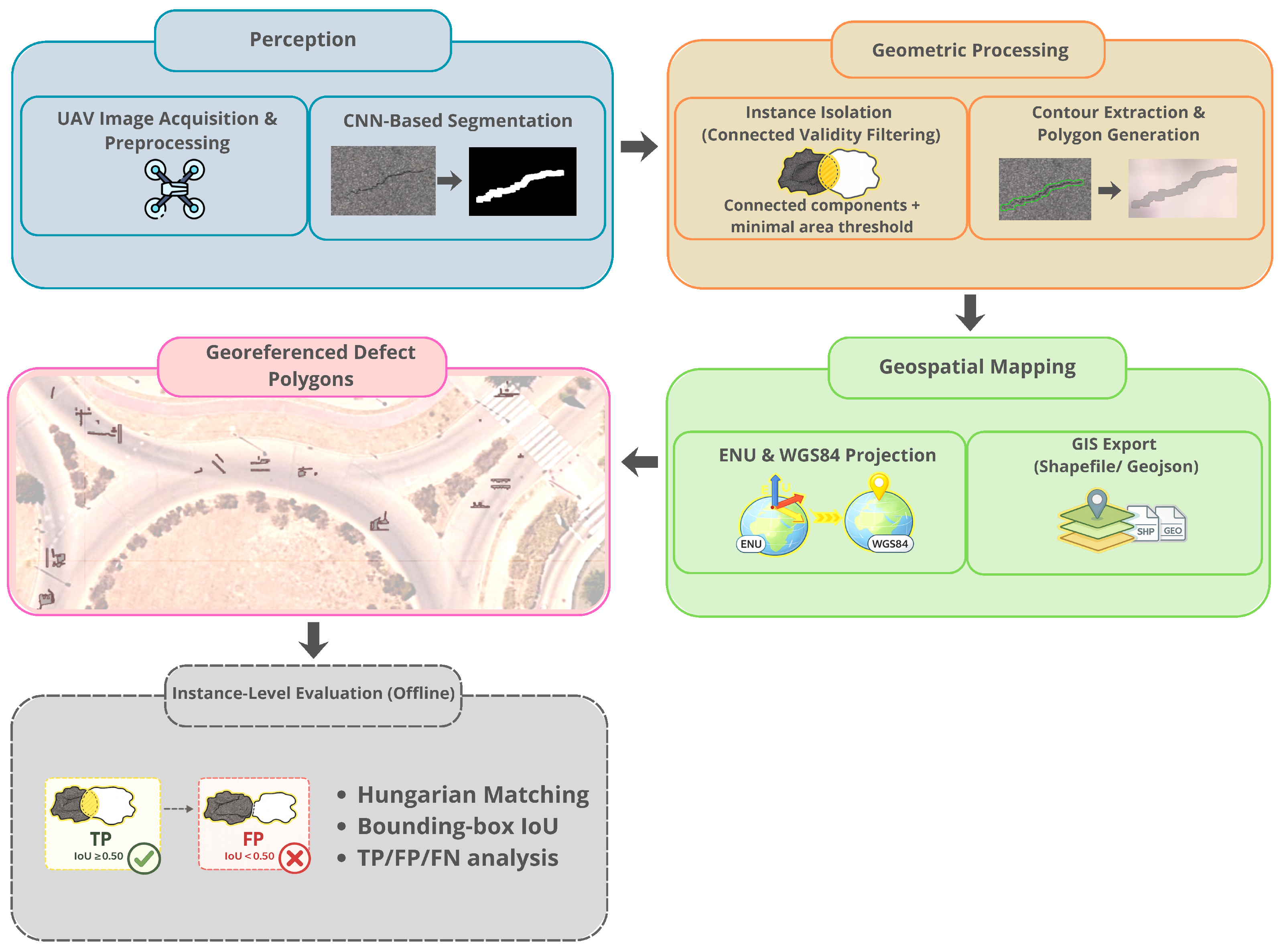
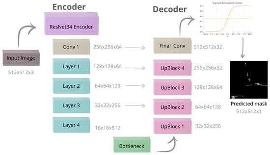
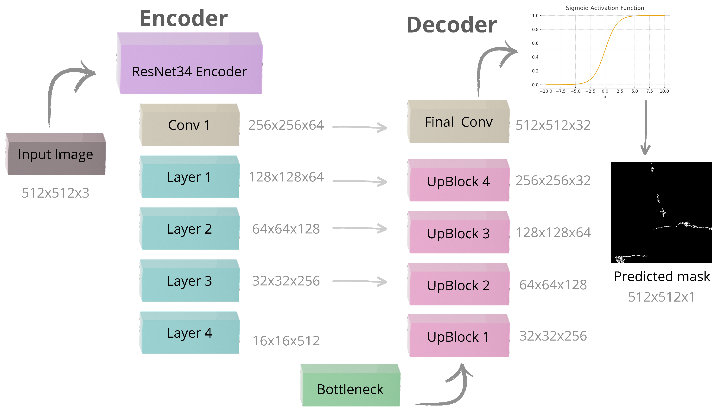
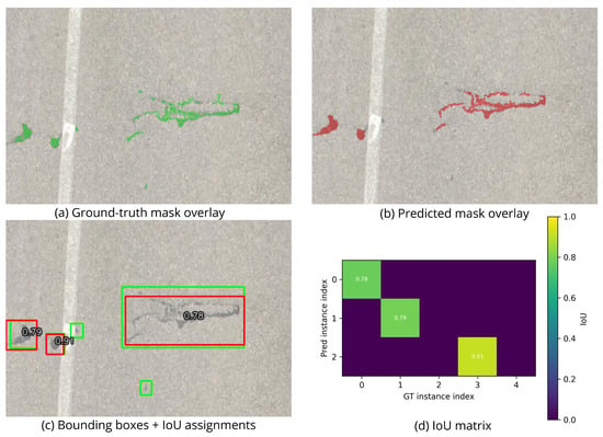
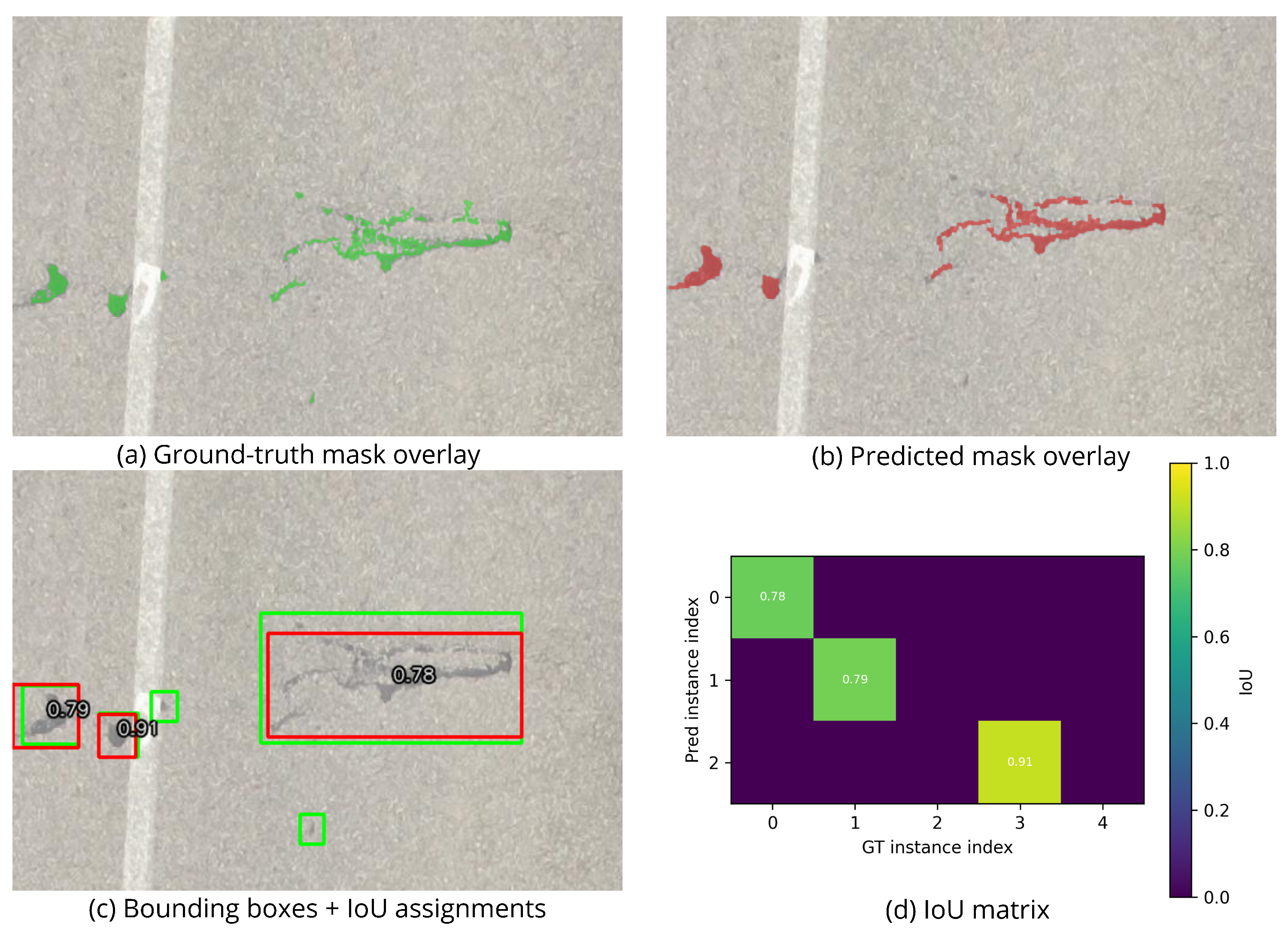
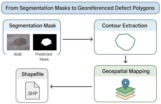
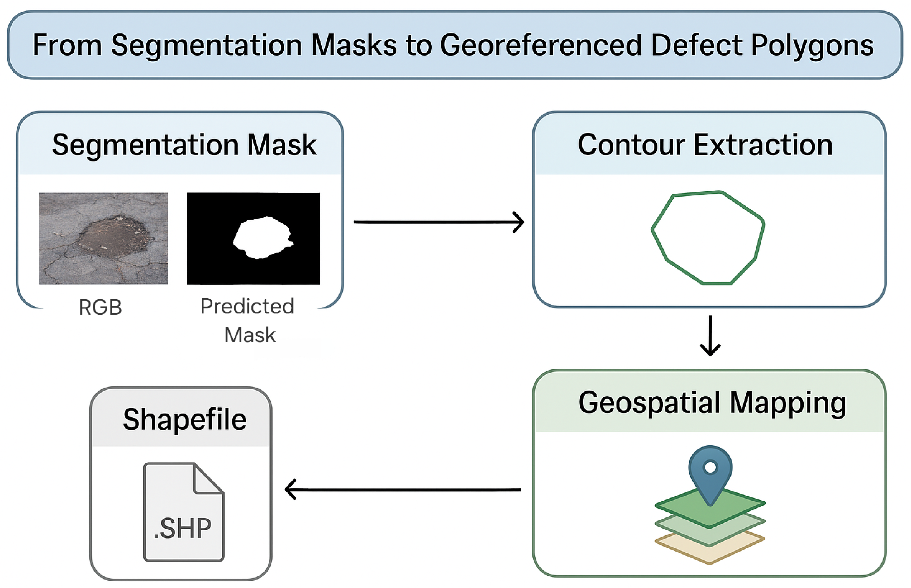
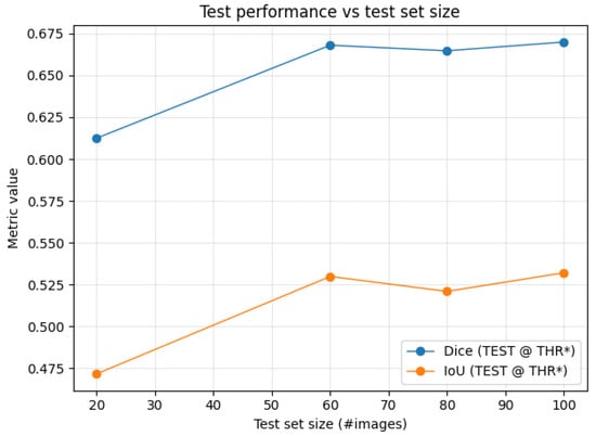
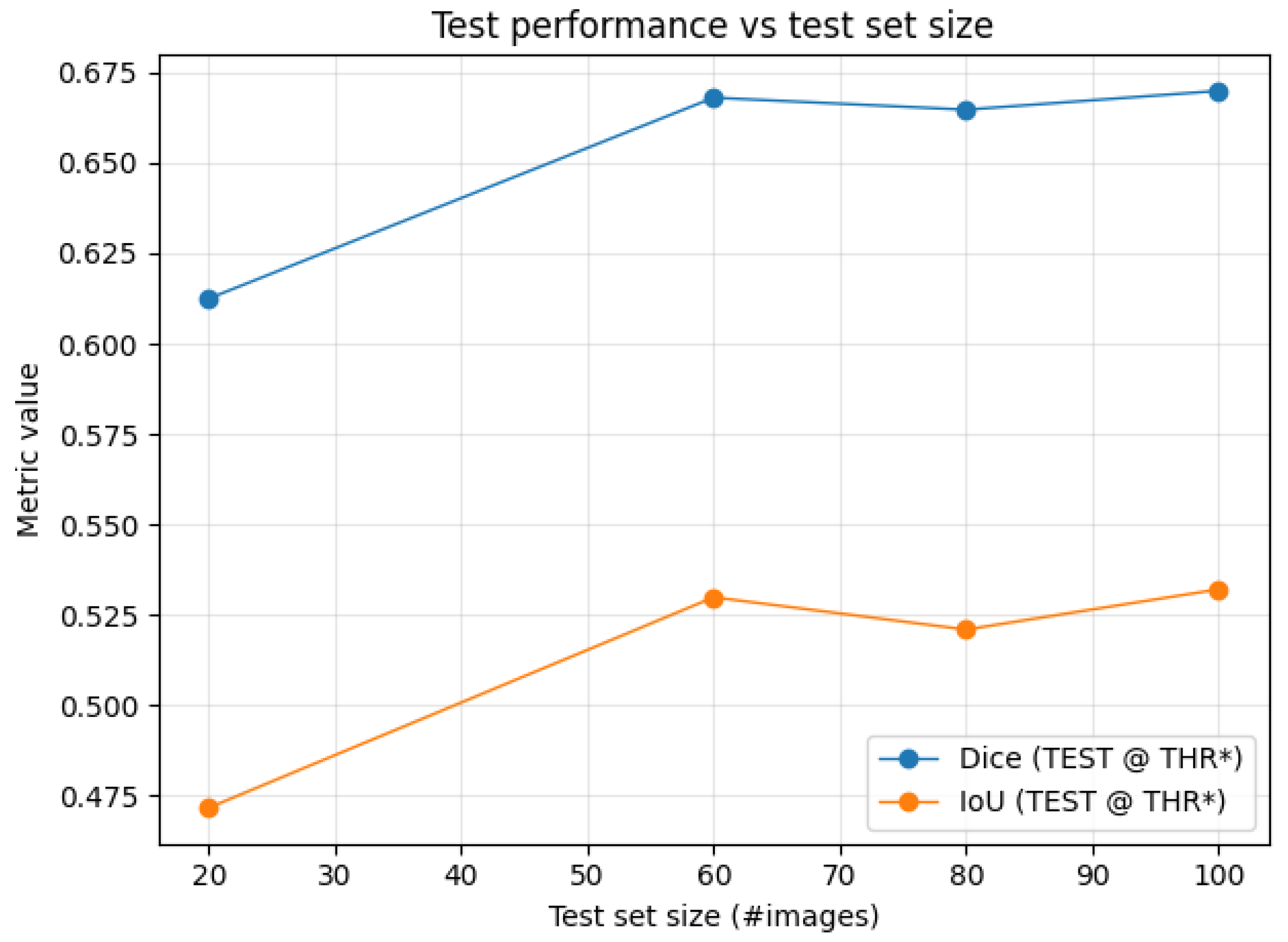
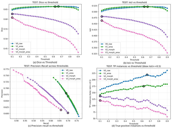
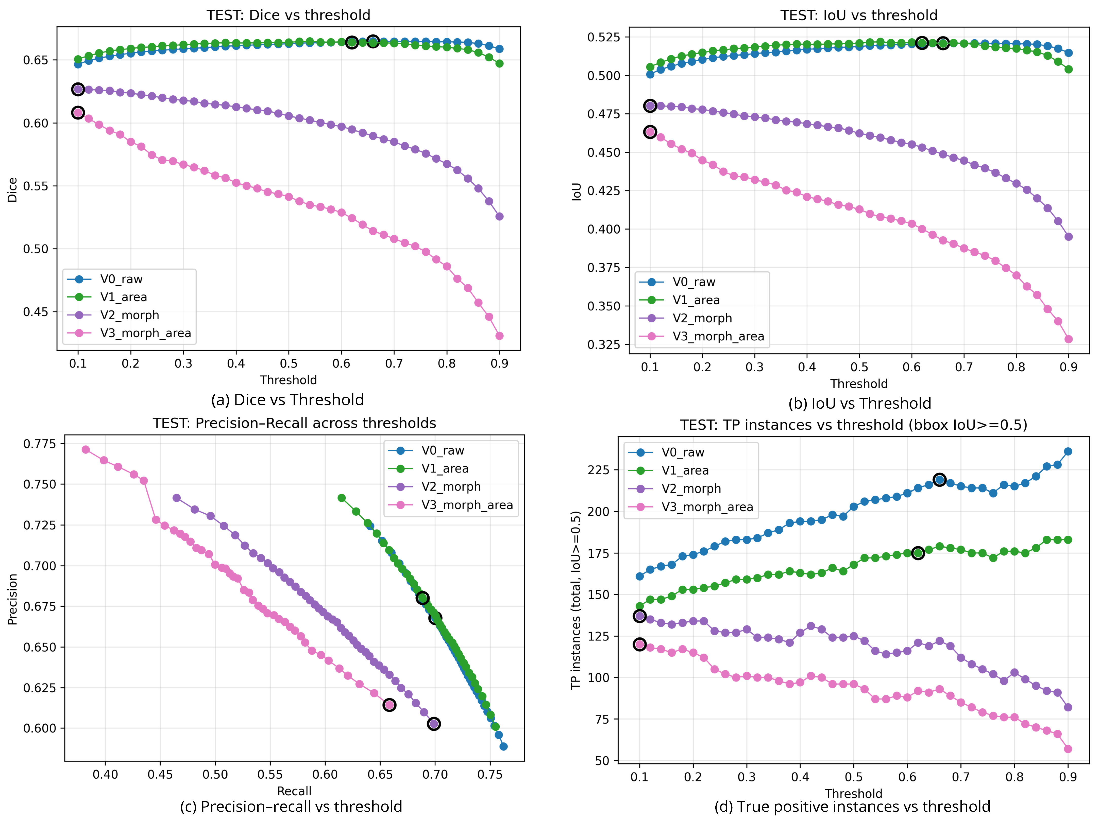
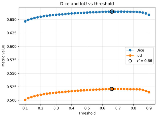
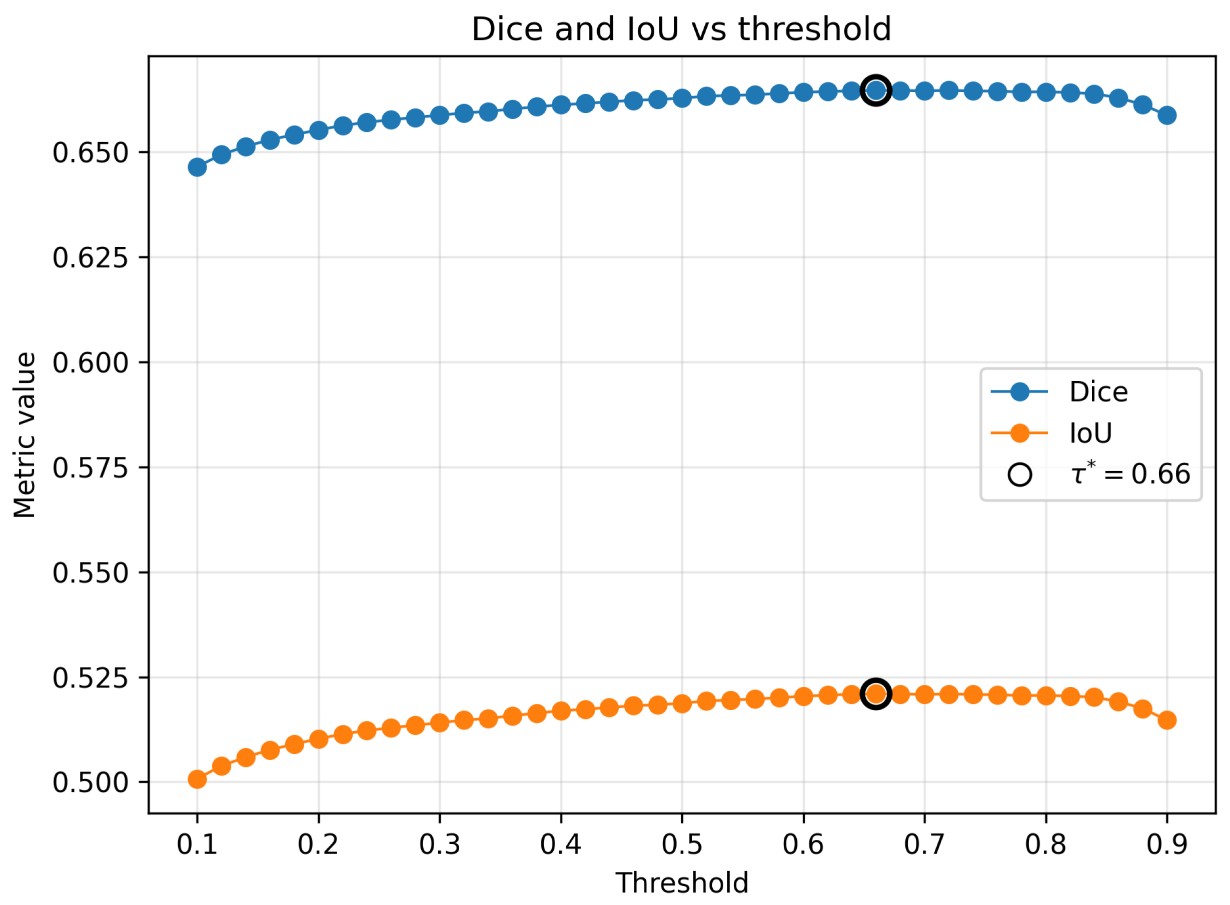
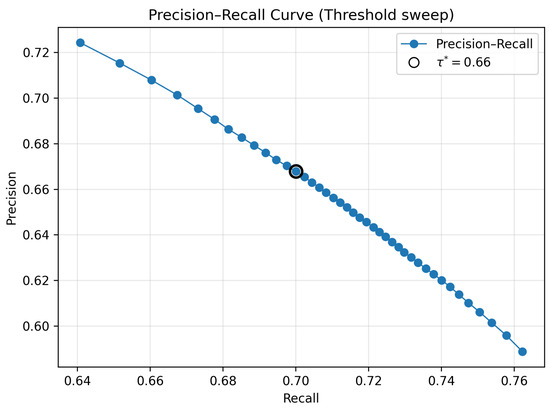
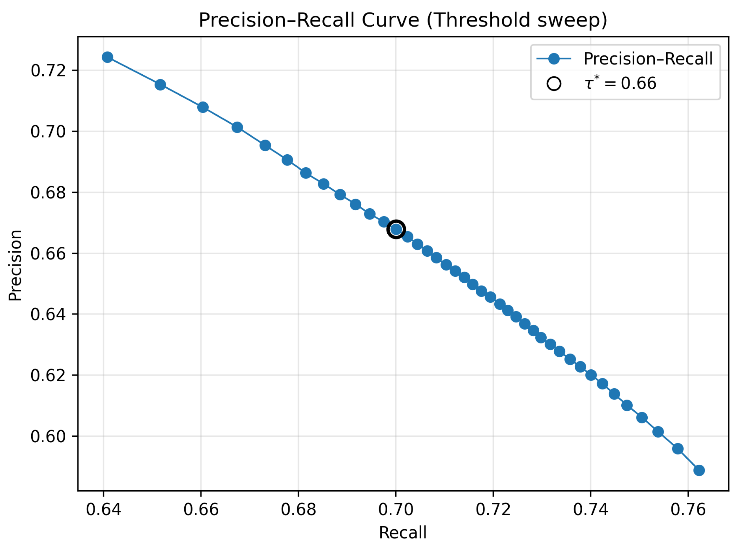
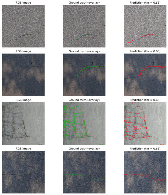
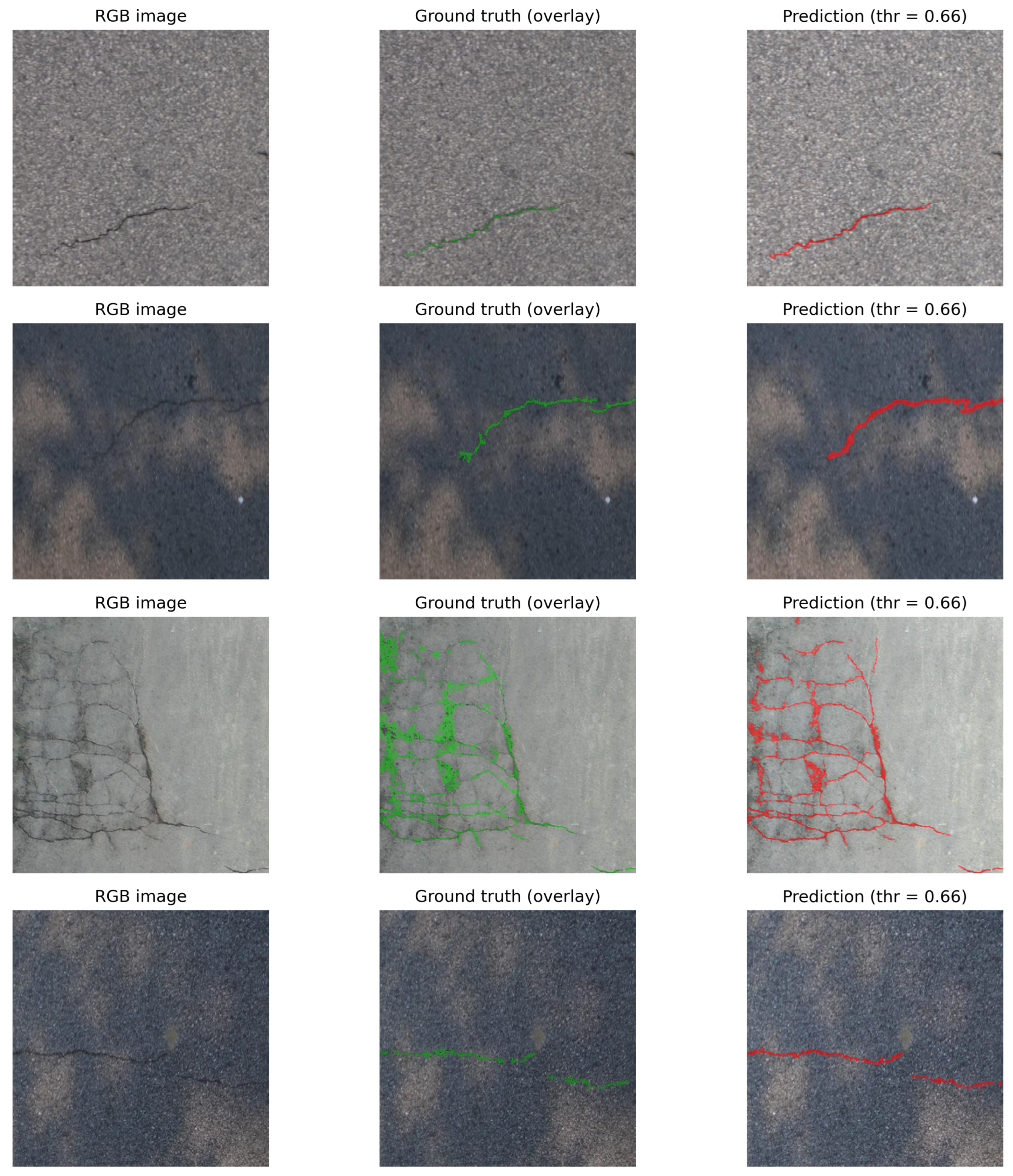
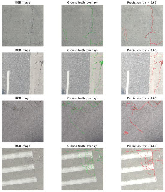
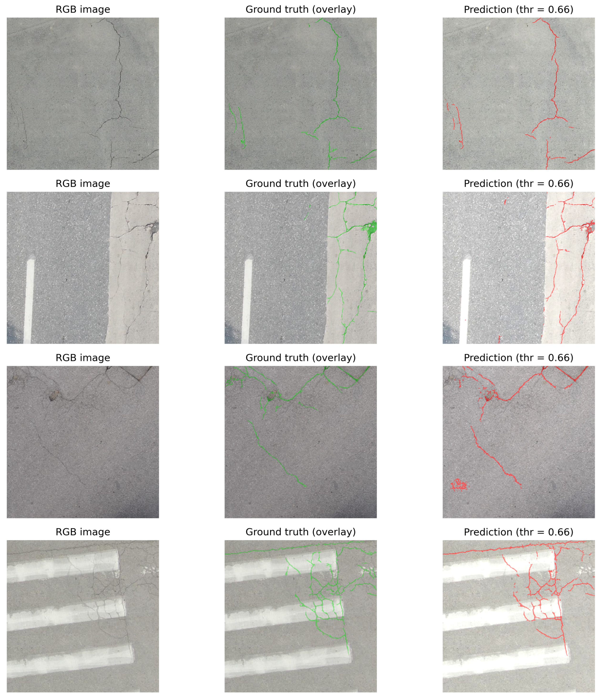
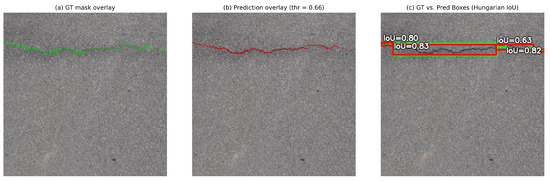
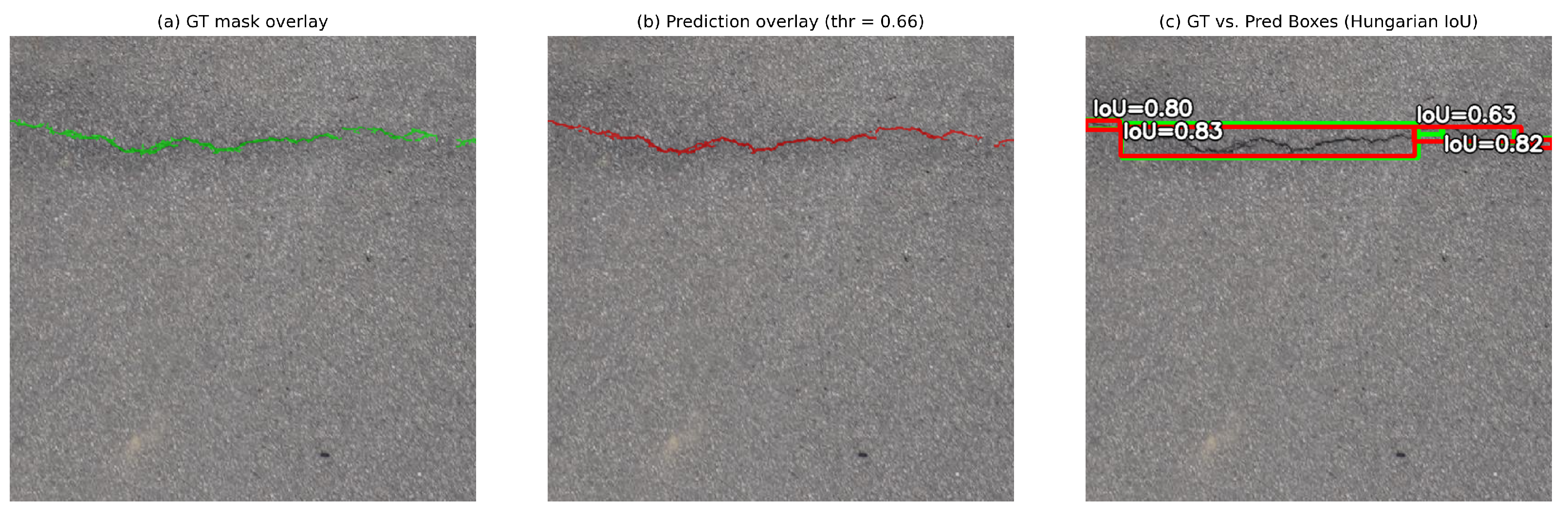
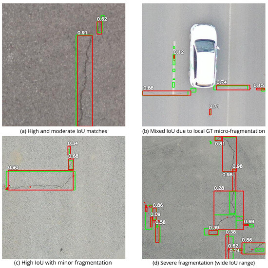
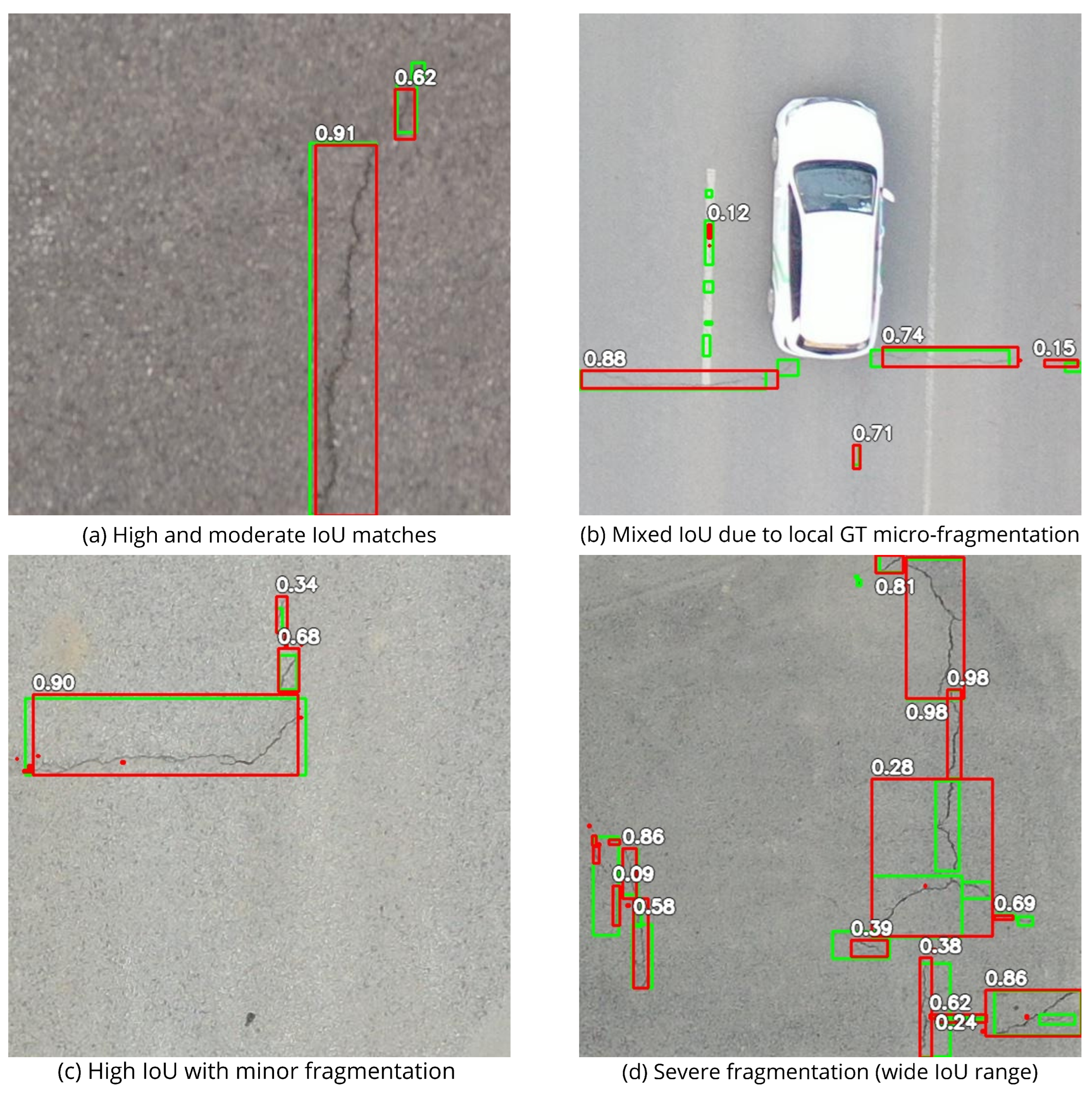
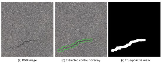
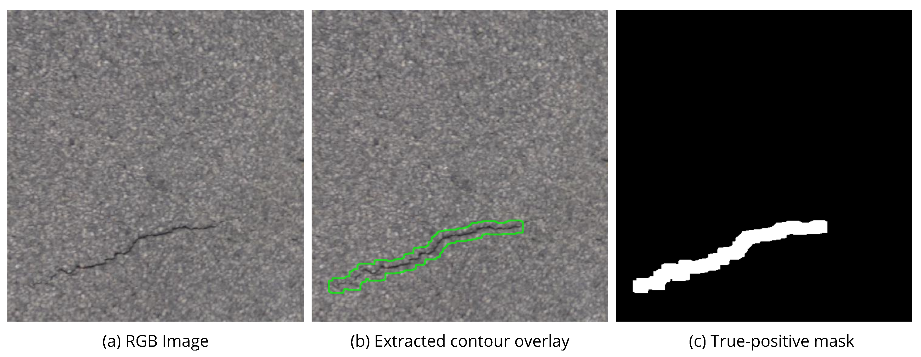
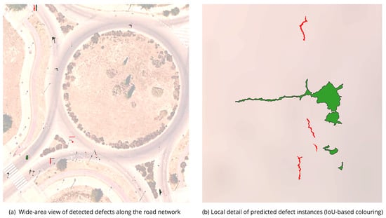
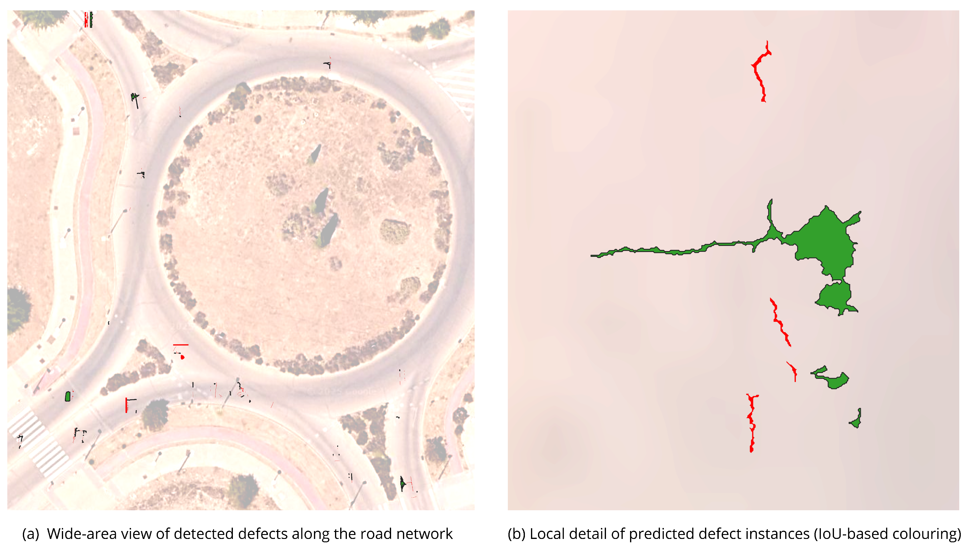
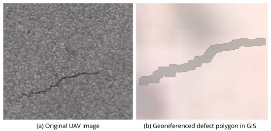
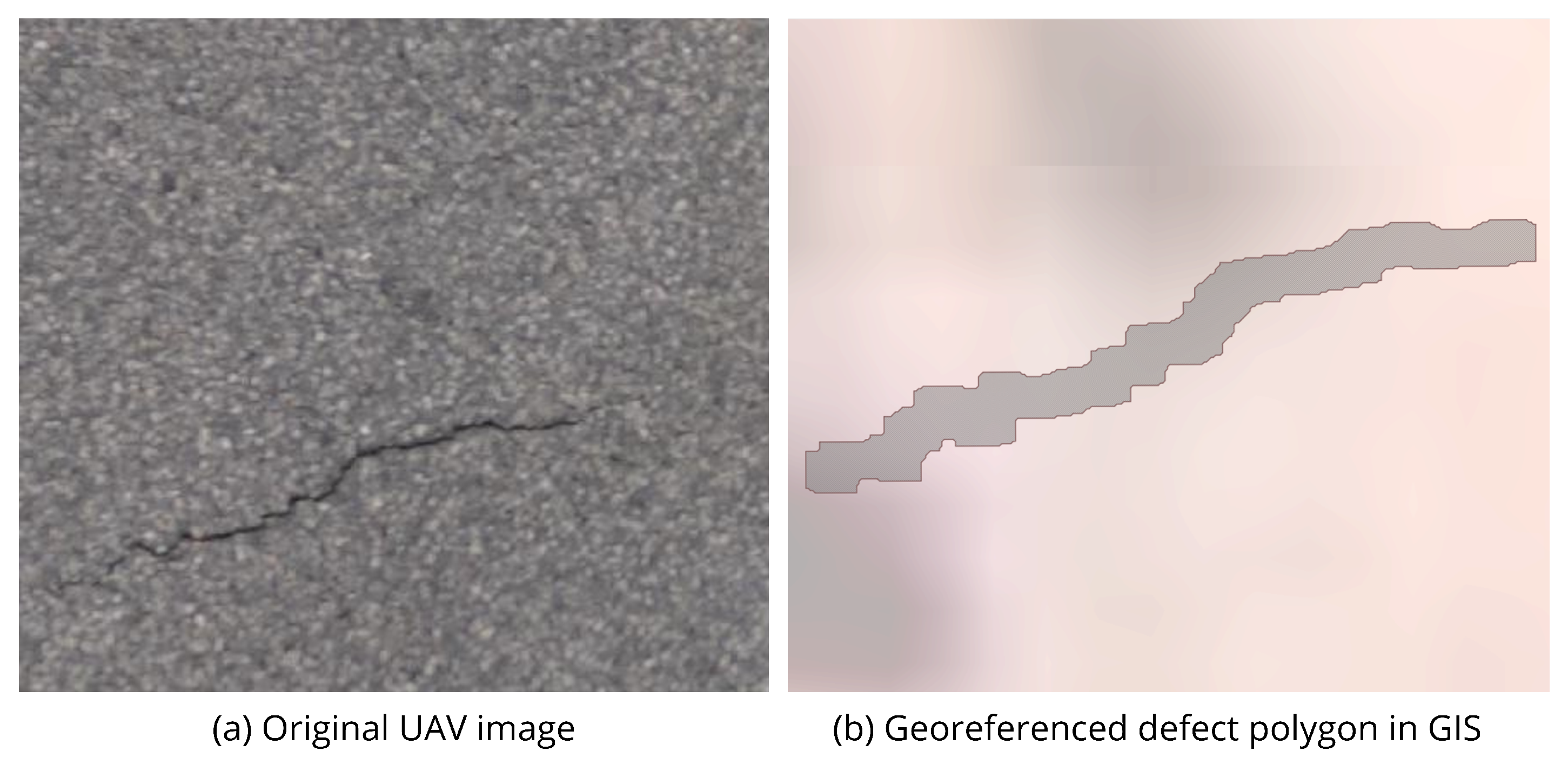
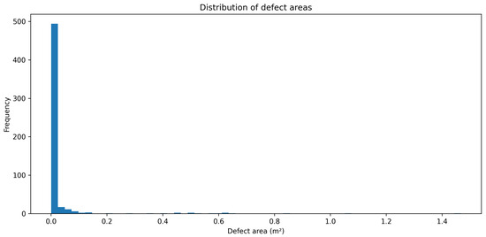
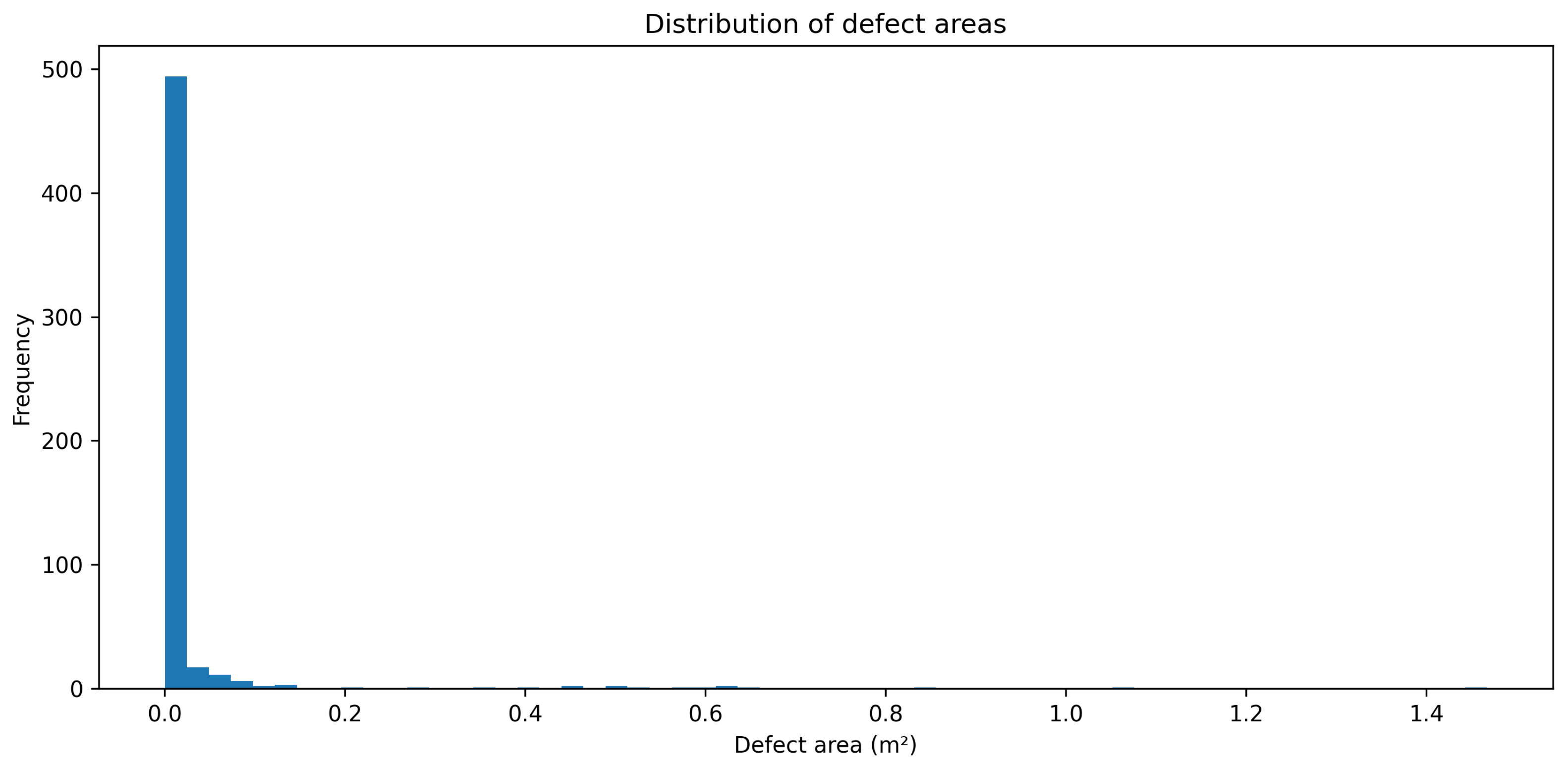
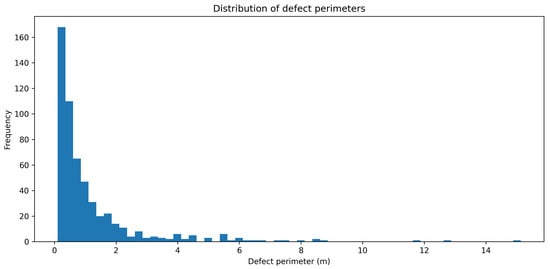
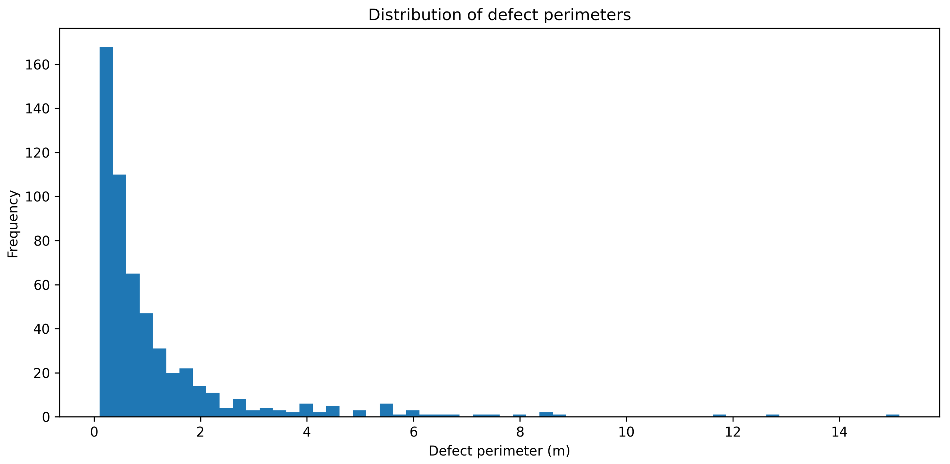

Disclaimer/Publisher’s Note: The statements, opinions and data contained in all publications are solely those of the individual author(s) and contributor(s) and not of MDPI and/or the editor(s). MDPI and/or the editor(s) disclaim responsibility for any injury to people or property resulting from any ideas, methods, instructions or products referred to in the content. |
© 2026 by the authors. Licensee MDPI, Basel, Switzerland. This article is an open access article distributed under the terms and conditions of the Creative Commons Attribution (CC BY) license.