


Highlights
What are the main findings?
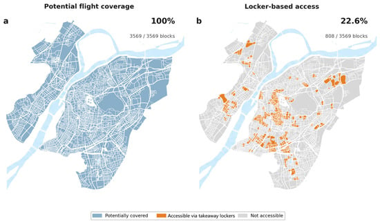
- Under the baseline configuration, UAV flight links potentially cover all 3569 blocks in central Nanjing; after accounting for pickup-locker locations and a 417 m walking condition, only 808 blocks (22.6%) have effective access.
- Across 81 infrastructure combinations, the mean standard deviational ellipse area of the simulated outlet distribution ranges from a 46.69% contraction to a 21.62% expansion relative to the road-delivery baseline, indicating configuration-dependent changes in the spatial distribution of supply.
What are the implication of the main findings?
- Pre-implementation assessment should follow the complete outlet–launch node–pickup locker–consumer chain and jointly examine aerial connectivity, last-mile access, and supply response.
- Within the tested configuration levels, pickup-locker configuration and flight-link distance show larger differences in SDE response; the walking radius mainly changes effective consumer access, while the launch-node configuration mainly changes outlet–node proximity.
Abstract
Urban drone delivery operates as a city-scale service network jointly structured by launch nodes, flight links, pickup lockers, pedestrian access, and outlet locations. Using 3569 street blocks and 21,366 food-delivery outlets in central Nanjing, this study develops an agent-based scenario model for pre-implementation assessment that links effective consumer access, node-level demand allocation, and outlet relocation and examines outlet-side access impedance together with 81 infrastructure configurations. Under the baseline configuration, flight links potentially cover all blocks, while only 22.6% satisfy the last-mile locker-access condition. Relative to the common road-delivery baseline, the standard deviational ellipse (SDE) area of the simulated outlet distribution contracts by a mean of 25.03% across ten runs, and the mean number of blocks with outlets decreases from 3460 to 3122.8. As outlet-to-node access impedance increases, the mean share of outlets within 1 km of launch nodes rises from 31.68% to 65.07%. Across the 81 configurations, mean SDE-area changes range from −46.69% to +21.62%. Within the tested levels, the pickup-locker configuration and flight-link distance are associated with larger differences in SDE response; walking radius mainly affects effective consumer access, whereas launch-node configuration mainly alters outlet–node proximity. The study provides a spatial screening framework for comparing urban drone-delivery networks along the complete delivery chain before detailed fleet, routing, and operational design.
1. Introduction
Online food-delivery platforms extend restaurant service areas and reshape spatial connections between outlets and consumer demand. Outlets can receive online orders from consumers beyond their walking distance, while the delivery distance, surrounding populations, and commercial centers remain important locational conditions. Research on platform-based food services has examined the spatial organization of outlets and their relationship with the local restaurant industry [1,2]. A micro-location study in Xinjiekou, Nanjing, further identified associations between platform outlets, commercial centers, and consumer demand, with locational differences across business types [3]. These existing locational relationships form the spatial context through which an urban drone-delivery network may influence food-service supply.
Unmanned aerial vehicle (UAV) delivery introduces a multi-stage service chain between outlets and consumers. Wing’s collaborations with Coles and Walmart demonstrate an operating model in which stores connect directly to drone-delivery networks [4,5]. Systems based on centralized launch operations and locker handoffs instead follow a continuous outlet–launch node–flight link–pickup locker–consumer path. Network-design studies have examined combinations of hubs, lockers, and drones [6,7,8]. Across configurations, service availability is jointly shaped by UAV ranges, relationships among supply and demand nodes, and handoff facilities. Meituan’s 2021 Corporate Social Responsibility Report describes couriers collecting goods from merchants for launch-site transfer, followed by drone transport to community stations and consumer collection from lockers [9] (p. 34).
Drone-logistics research has developed extensive routing-optimization and facility-location methods [10,11]. Reviews have further synthesized optimization approaches, technological trends, and operational constraints in last-mile drone delivery [12,13]. From a spatial perspective, He et al. [14] analyzed the spatial heterogeneity of Hangzhou’s UAV logistics network and its associated factors, while Wang et al. [15] compared urban morphology and simulated drone-logistics network costs across 101 Chinese cities. Existing work therefore provides a strong methodological basis for network design and performance assessment, although the systematic analysis of how urban food-delivery supply may respond spatially after a new network is introduced remains comparatively limited. Straubinger et al. [16] examined long-term urban spatial equilibrium under e-commerce and drone delivery, while He et al. [17] modeled restaurant quality, location, and platform competition. The present model holds population and outlet totals fixed to examine location responses to specific launch-node and locker connections.
Flight radius primarily describes the aerial-connection range. The broader spatial response also depends on opportunities, transport impedance, and the spatial arrangement of supply and demand [18,19]. Online food-delivery research shows that spatial disparities in food access persist within digital services [20,21]. Under locker-based handoffs, a consumer block can enter the service network only when a connected pickup facility lies within walking range, while the demand available to an outlet further depends on node allocation and access impedance. Potential flight coverage, effective consumer access, node demand, and supply redistribution therefore need to be measured separately along the complete delivery chain.
This study uses central Nanjing as the study area and combines existing population, food-delivery outlet, road-network, and facility data to develop an agent-based scenario assessment for pre-implementation evaluation. Whereas drone-network design studies commonly treat supply and demand locations as given, this study further examines how food-delivery outlet locations may respond spatially to changes in network configuration. Three questions guide the analysis. First, how much effective service coverage remains when locker and walking constraints are imposed on potential UAV coverage, and how does the simulated outlet distribution respond? Second, how do node proximity and the spatial extent of the outlet distribution change as outlet-to-launch-node access impedance increases? Third, how do combinations of the flight-link distance, walking pickup radius, pickup lockers, and launch nodes alter service access and supply response? By linking infrastructure configuration, node-level demand allocation, and outlet relocation, the analysis provides a spatial screening approach for comparing urban drone-delivery networks before detailed fleet, routing, and operational designs.
2. Materials and Methods
2.1. Analytical Framework
The analysis proceeds through the diagnosis of observed supply, a construction of a road-delivery baseline, and a simulation of drone-delivery scenarios. A hurdle random forest first characterizes relationships between the observed outlet distribution and population, roads, and center–periphery position. An agent-based model is then run under a 6 km road-delivery rule. When outlet relocations satisfy the predefined stopping criterion, the resulting distribution is used as the common initial state and road-delivery baseline for all core drone-delivery scenarios. Each infrastructure network is simulated independently from this baseline, allowing comparison of spatial outcomes under the same stopping rule. Agent-based methods represent spatial responses through repeated locational adjustments and have been applied to urban logistics comparisons [22,23]. Population demand, block units, and the citywide outlet total remain fixed, so the analysis focuses on relative spatial outcomes under changing drone-network connections and outlet access conditions.
2.2. Study Area and Spatial Data
The study area is central Nanjing, comprising the main urban area south of the Yangtze River and the new urban area north of it, with a planned area of approximately 808 km2 [24]. The old city, new urban districts, and riverside clusters differ in population, food-service supply, commercial centers, and road conditions. Previous research has documented spatial differences in online food accessibility across areas and population groups in Nanjing [25]. These internal differences in supply, demand, and spatial structure allow comparison of responses to the same drone-delivery rules across urban districts.
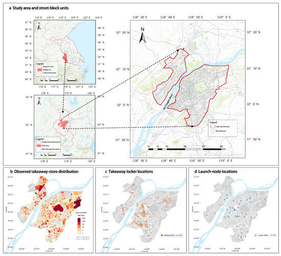
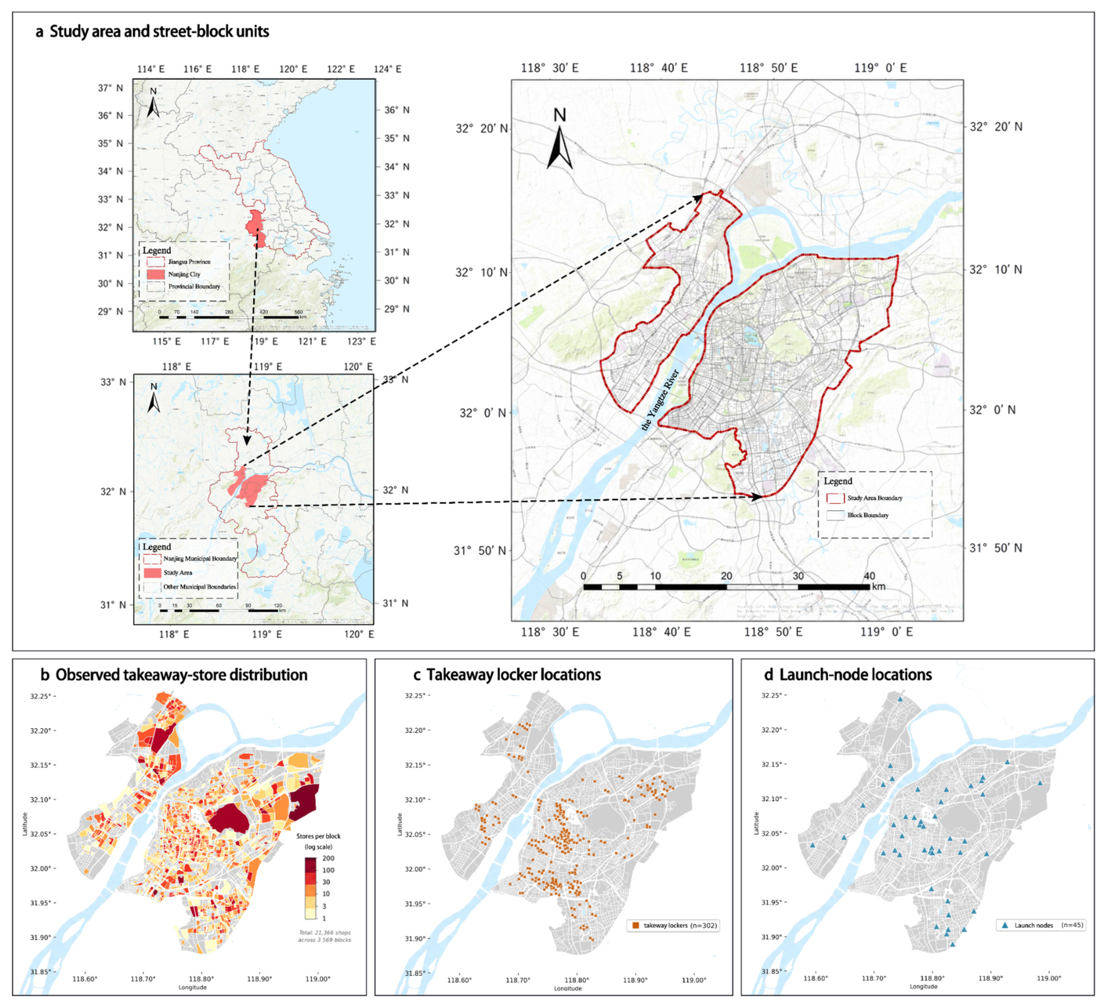
The analysis and simulation use 3569 street blocks as the common spatial unit. The 2025 spatial database includes block boundaries, food-delivery points of interest (POIs); anonymized mobile-signaling population data; the road network; central business districts and commercial centers; and takeaway lockers, smart lockers, and other related pickup-facility POIs. Population is aggregated to blocks to represent potential consumer demand, while outlet counts represent supply and the simulation state. The OpenStreetMap road network is used to calculate shortest road distances between blocks. POIs are obtained from the Amap Open Platform; filtering, deduplication, and spatial matching retain 21,366 food-delivery outlets. Figure 1 shows the study area and data distributions.
Figure 1.
Study area, food-delivery outlets, and baseline facility proxies.
Baseline infrastructure comprises 45 launch-node proxies and 302 pickup-facility proxies. Launch-node proxies are selected from CBD, shopping-center, and commercial-complex POIs, while pickup facilities are assembled from takeaway-locker, smart-locker, and related facility POIs. These locations define the drone-delivery networks to be evaluated. Reduced configurations use each replicate’s seed to sample 23 launch nodes and 151 lockers from the respective baseline sets. The 60-node configuration retains the original 45 nodes and adds 15 fixed peripheral proxy locations. The 604-locker configuration retains the original 302 locations and adds 302 block-centroid proxies in descending population order, preferentially selecting locations more than 500 m from existing lockers. Table S1 documents data processing and facility-construction rules.
Of the observed blocks, 1954 (54.7%) contain no food-delivery outlets. A two-stage hurdle random forest addresses these zeros: a classifier estimates outlet presence, and a regressor estimates outlet counts among nonzero blocks [26,27,28]. Explanatory variables include the straight-line distance in UTM coordinates to a fixed central reference point (118.796 °E, 32.060 °N), with population covered by road delivery, road density, and the mean outlet count of adjacent blocks. Classification accuracy, regression R2 for nonzero blocks, an overall Spearman correlation, and total predicted outlets are used to evaluate in-sample fit. The model describes spatial relationships in the observed distribution; the subsequent relocation model uses separately specified behavioral rules. The expected outlet count is the product of predicted presence probability and predicted positive count; Equation (S5) and the fitting settings are given in Supplementary Method S1.
2.3. Delivery Paths and Effective Accessibility
Road-delivery connections are defined by the shortest road distance between outlet and consumer blocks, with a connection established at distances no greater than 6 km. This threshold is used as a common comparison condition and is informed by food-delivery time constraints and courier cycling characteristics [29,30]. Delivery extent is represented by a distance threshold; waiting, intersection delays, and order-level travel times are left to finer-scale transport simulation. Wang and He [31] reported a 6 km reference range containing approximately 95.5% of delivery trips in the data they cited; Liu et al. [32] also used a 6 km demand-search range in Shanghai.
Drone delivery follows an outlet–launch node–pickup locker–consumer connection path. Each outlet block is assigned to its nearest launch node. A feasible outlet–consumer connection exists when a pickup locker lies within that node’s flight-link distance and the consumer block lies within the walking radius of the same locker. Launch nodes and lockers provide handoffs between transport stages, an organization discussed in relay-based drone-network research [33]. Outlet-to-node distance is examined separately in the access-impedance sensitivity analysis. Node–locker and block centroid–locker distances are UTM planar straight-line distances. A consumer block and its entire population are counted when its centroid satisfies the locker-access condition; the latter distance approximates walking access.
The UAV transport stage is represented at the network-configuration level. A flight link is recorded when the straight-line distance between a launch node and a pickup locker does not exceed the specified threshold. Operating scenarios assess fleet, queueing, charging, and endurance constraints through discrete-event simulation. Orders wait for an idle drone and a charged battery; returned batteries queue for charging. At node a, qₐ is the fraction of arriving orders delivered within 30 min of node arrival under the round-trip flight budget after a 20% reserve. Effective demand, expressed as where Dₐ is allocated node demand, enters the benefit and relocation rules in Section 2.4 to simulate outlet distributions. Fulfillment fractions remain fixed during location updates; unfulfilled demand is not reassigned. The core model uses qₐ = 1; the full settings are in Supplementary Method S3 and Table S13.
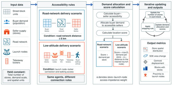
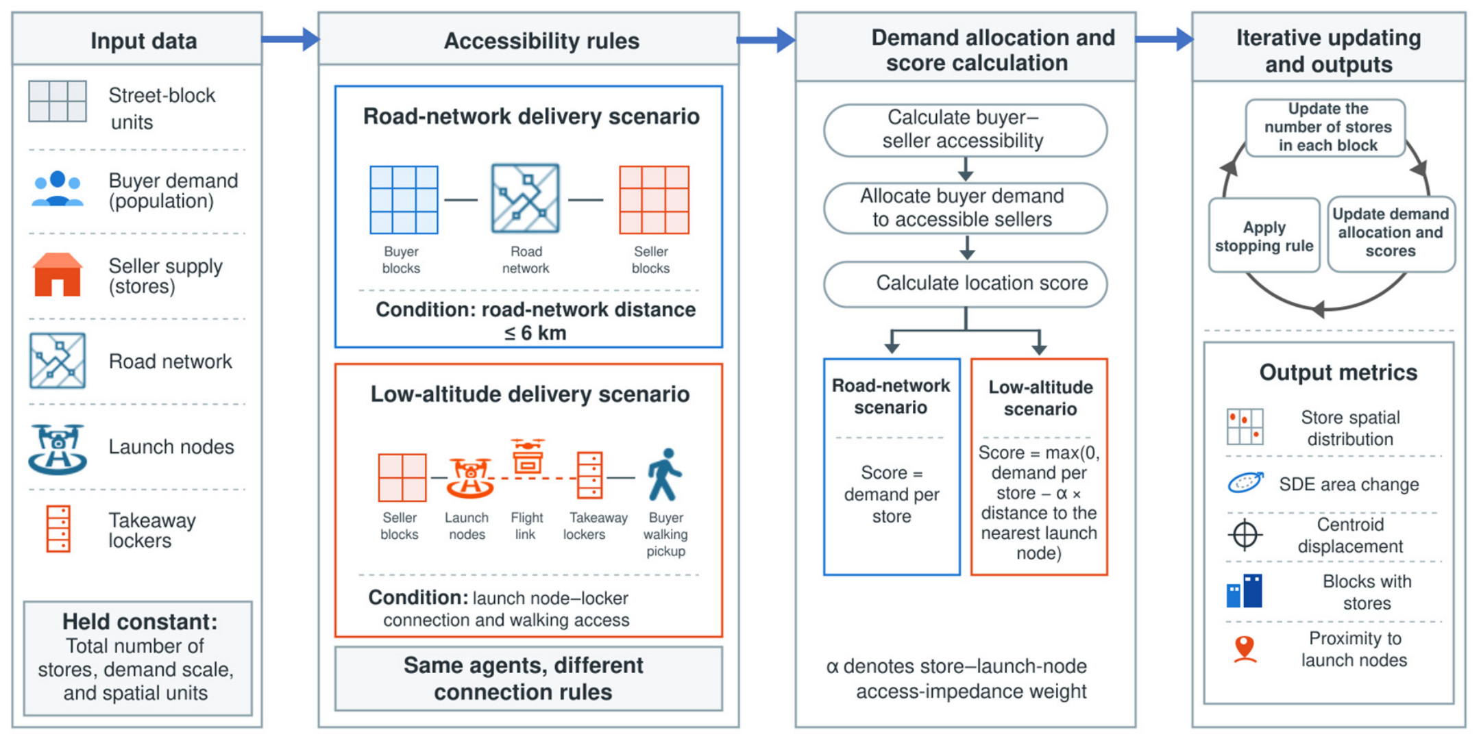
We let Rij denote accessibility between consumer block i and outlet block j; Rij = 1 when the corresponding delivery-path conditions are met, and 0 if otherwise. Potential flight coverage denotes blocks covered under the specified flight threshold. Effective consumer access additionally requires a connected pickup locker within walking range. The demand available to an outlet depends on which consumers can be served by its assigned node. These measures describe UAV flight coverage, last-mile access, and outlet service connections. Supplementary Method S1 and Equations (S1)–(S4) formalize road access, nearest-node assignment, node–consumer connections, and outlet–consumer access. Figure 2 summarizes the delivery connections and the agent-based scenario framework.
Figure 2.
Delivery connections and agent-based scenario framework. In the drone-delivery scenarios, demand is first aggregated to launch nodes able to serve consumers and then allocated to outlets assigned to those nodes; benefit updating and relocation rules are described in Section 2.4.
2.4. Outlet Relocation and the Common Baseline
Block population represents demand and block outlet counts represent supply. Outlets can relocate between blocks while the citywide total remains fixed at 21,366. The road simulation starts with a preliminary outlet distribution generated with the aid of processed population-coverage and central-distance response curves and runs under the 6 km road-delivery rule until outlet relocations satisfy the predefined stopping criterion. Under the road rule, each consumer block’s population is shared equally among all reachable supply blocks, including empty blocks; allocated block demand divided by its outlet count gives the current score when occupied. The resulting distribution serves as the road-delivery baseline. Each core drone-delivery scenario starts independently from this baseline with the same population distribution and random seed, preventing one infrastructure configuration from inheriting relocation outcomes from another. Nodes and lockers remain fixed within each run. The comparison replaces the road allocation mechanism with the low-altitude mechanism for the fixed outlet total; all infrastructure scenarios share this adopted condition.
Demand in the drone-delivery network is organized by node. The population of each consumer block is divided equally among all launch nodes that can serve it through pickup lockers, and these allocations are aggregated into the node demand. Outlet blocks connect to their nearest launch node. Dividing node demand by the total number of outlets connected to that node gives a node-level per-outlet benefit. For an occupied block j in round t, the net score is
Here, h(j) is its nearest node, Dh(j) is the allocated node demand, Nh(j)(t) is the attached outlet count, dj,h(j) is the distance to that node in kilometers, and α is defined below. The model updates historical benefits for blocks containing outlets and applies a local competition adjustment based on block outlet counts when evaluating current locations. Specifically, the current-block score divides the nonnegative net node benefit once more by the local outlet count, whereas a candidate uses its historical mean net benefit over occupied rounds. Road histories use cumulative allocated block demand divided by cumulative outlet counts over occupied rounds. Initial historical scores are 0 for road delivery and 0.1 for low-altitude delivery. Equations (S6)–(S9) and the pseudocode in Supplementary Method S1 specify the road admission, empty-node handling, round-start scoring, and round-end updating.
Outlets relocate probabilistically. Initial relocation and exploration probabilities are 0.15 and 0.10, respectively, and both are multiplied by 0.97 each round, with a lower bound of 0.001. During low-altitude exploration, outlets may move to blocks with positive historical benefits. Otherwise, five candidate blocks are sampled, and relocation occurs when the highest historical benefit exceeds the current-location score. Road candidates additionally require their provisional outlet count to be below their historical score; road exploration samples one block uniformly under this condition. Both stages compute scores and histories from the distribution at the start of each round and apply accumulated relocations at its end. Simulations of the 81 infrastructure configurations terminate when the mean relocations over the latest 30 rounds fall below 1% of the citywide outlet total, with a maximum of 2000 rounds using seeds 1–9 and 42. Rounds denote location updates rather than calendar time. As the probability schedule reduces search activity, the stopping rule defines comparable endpoints under that schedule; sensitivity to alternative schedules is reported in Table S9.
Outlet-side access impedance is represented by α. With baseline facilities fixed, α takes values of 0, 0.1, 0.5, 1, 2, 5, 10, and 20 to examine how outlet distributions respond as the locational disadvantage of being farther from launch nodes increases. α is the score deduction per kilometer of outlet-to-node distance; its levels define comparative distance-impedance scenarios under the specified relocation rules.
2.5. Scenario Design
The baseline drone-delivery scenario uses 45 launch nodes, 302 pickup lockers, a 10 km flight-link distance, a 417 m walking pickup radius, and α = 0. The 417 m radius approximates a five-minute one-way walk at an assumed 5 km/h and defines the baseline pickup condition; 250 and 800 m represent stricter and more permissive spatial-access conditions. Three levels each of flight-link distance, walking radius, locker configuration, and launch-node configuration form 81 full-factorial scenarios; all infrastructure-combination experiments use α = 0. One-factor contrasts are extracted directly from these 81 scenarios while holding all other infrastructure parameters at baseline levels (Table 1). Complete configurations and outputs are reported in Table S2a–c, with parameter rationales in Table S5 [34,35,36]. Each configuration and α level is repeated ten times with seeds 1–9 and 42; the experiments share the baseline α = 0 across runs. Tables report means and sample standard deviations, with 95% mean confidence intervals for α and selected controls. Maps and single-run network examples are labeled seed 42. Supplementary Methods S1–S3 describe controls for the observed starting states, initialization, node layouts, demand allocation, relocation parameters, and operating conditions [37,38,39].
Table 1.
Scenario settings and controlled conditions.
2.6. Evaluation Metrics
Evaluation covers effective service coverage, network organization, and spatial supply response (Table 2). Effective-access blocks and their population represent potential demand able to enter the service through pickup lockers. Node–locker edges and unconnected lockers describe aerial-network connectivity. The node-demand Gini coefficient is calculated from node demand after each consumer block’s population has been divided equally among serving nodes, and describes the balance of demand across nodes [40]. Multiple lockers connecting the same consumer block and node count once, and zero-demand nodes are included. Connection-overlap percentages accompany the Gini coefficient (Table S11), with units and denominators in Table S12; population coverage is also reported as a share of the total study-area population.
Table 2.
Evaluation metrics and reference distributions.
Spatial supply response is described using outlet-count-weighted centroids, standard deviational ellipses (SDEs), blocks with outlets, and node proximity. The SDE summarizes the spatial extent and orientation of the outlet distribution [41], and all centroid displacements are measured relative to the observed distribution. Ellipse-area changes use two reference comparisons: the road-delivery baseline relative to observations, and each core drone-delivery scenario relative to the common road-delivery baseline:
Here, Aobs, Aroad, and As denote ellipse areas for the observed distribution, road-delivery baseline, and drone-delivery scenario s, respectively. For observed-start controls, Aroad denotes the matched road endpoint. Negative ΔAs indicates contraction relative to the road-delivery baseline, while positive values indicate expansion. Node proximity includes the outlet-count-weighted mean distance to the nearest launch node and the share of outlets within 1 km of nodes. Spearman correlations between the road baseline and observed outlet counts are also calculated at block and 1 km grid scales to examine spatial consistency [42]. For each seed and infrastructure factor, SDE responses are averaged at each level over all combinations of the other factors; the largest minus the smallest level mean gives the marginal response range (Table S10). Local distribution differences are the sum of absolute outlet-count differences between matched 1 km grids divided by twice the total outlet count. Supplementary Method S2 details this measure and single-block-removal checks; Table S4e,f report these with the full ellipse axes and block occupancy.
Spatial processing uses ArcGIS 10.8 (Esri, Redlands, CA, USA). Original model calculations use Python 3.7.3 (Python Software Foundation, Beaverton, OR, USA) with GeoPandas 0.10.2, NetworkX 2.6.3, scikit-learn 1.0.2, SciPy 1.7.3, and Matplotlib 3.5.3; repeated simulations and statistical postprocessing use Python 3.12.14 (Python Software Foundation, Beaverton, OR, USA) (Table S5).
3. Results
3.1. Observed Supply Characteristics and the Road-Delivery Baseline
A hurdle random forest is first used to characterize relationships between the observed outlet distribution and road-delivery population coverage, central location, and other spatial conditions. In-sample outlet-presence classification accuracy is 0.873, regression R2 for nonzero blocks is 0.779, the overall Spearman correlation is 0.601, and the total predicted supply is 21,203 outlets. The distance to the fixed central reference point and road-delivery population coverage account for 44.7% and 41.0% of the classifier importance, respectively, followed by road density at 14.2%; the contribution of mean adjacent-block outlet counts is close to zero (Figure S1).
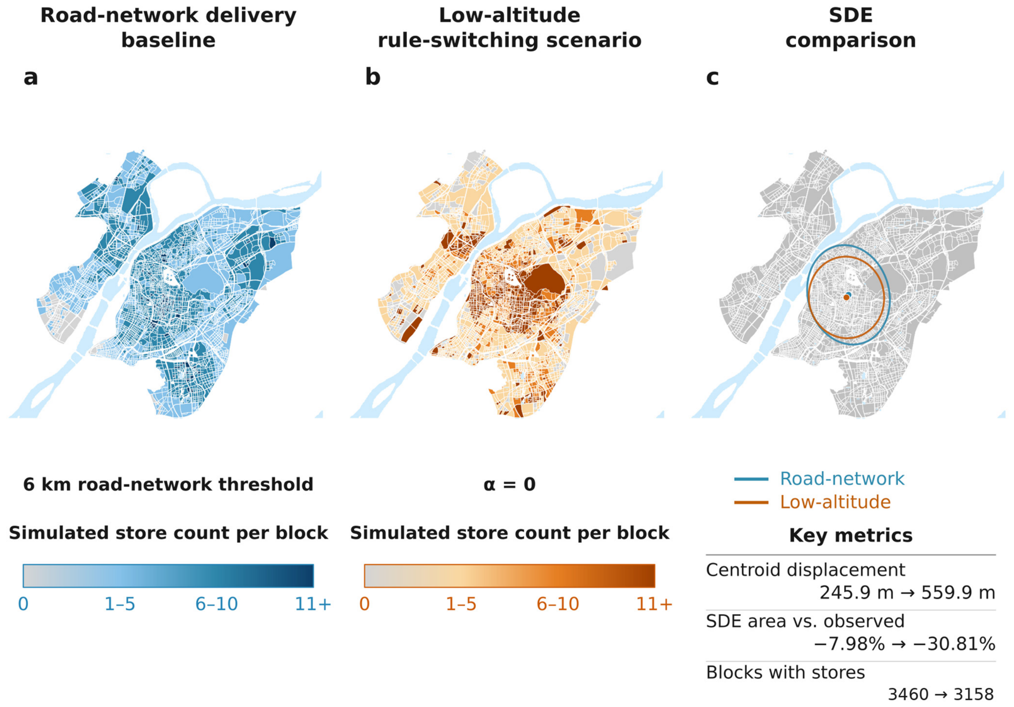
Processed population-coverage and central-distance response curves are used to generate a preliminary outlet distribution, which is then adjusted under road-delivery rules to obtain the common comparison baseline. Its SDE area is 159.48 km2, 7.98% smaller than the observed 173.32 km2, with a centroid displacement of 245.9 m. Blocks with outlets increase from 1615 to 3460, accounting for 96.9% of all blocks. The road baseline therefore combines a modest contraction in the overall spatial extent with broader block occupancy. Spearman correlation between simulated and observed counts is 0.2066 at the block scale and 0.5891 after aggregation to a 1 km grid, indicating that the road baseline retains some spatial correspondence at the grid scale, while discrepancies in outlet counts are concentrated at finer spatial resolution. To test the influence of this difference, road and low-altitude models either start separately from observations or are run sequentially from observations, with ten matched seeds under the baseline infrastructure at α = 0. Road endpoints retain 1606.7 occupied blocks on average and a block-level correlation of 0.8924. Relative to the matched road endpoints, the mean low-altitude area changes by −8.48% and −7.70% compared to −25.03% from the common baseline; occupied blocks increase in both controls (Table S6). Thus, overall contraction is retained, while its magnitude and occupancy response depend on the starting distribution.
3.2. Effective Service Coverage of the Baseline Drone-Delivery Network
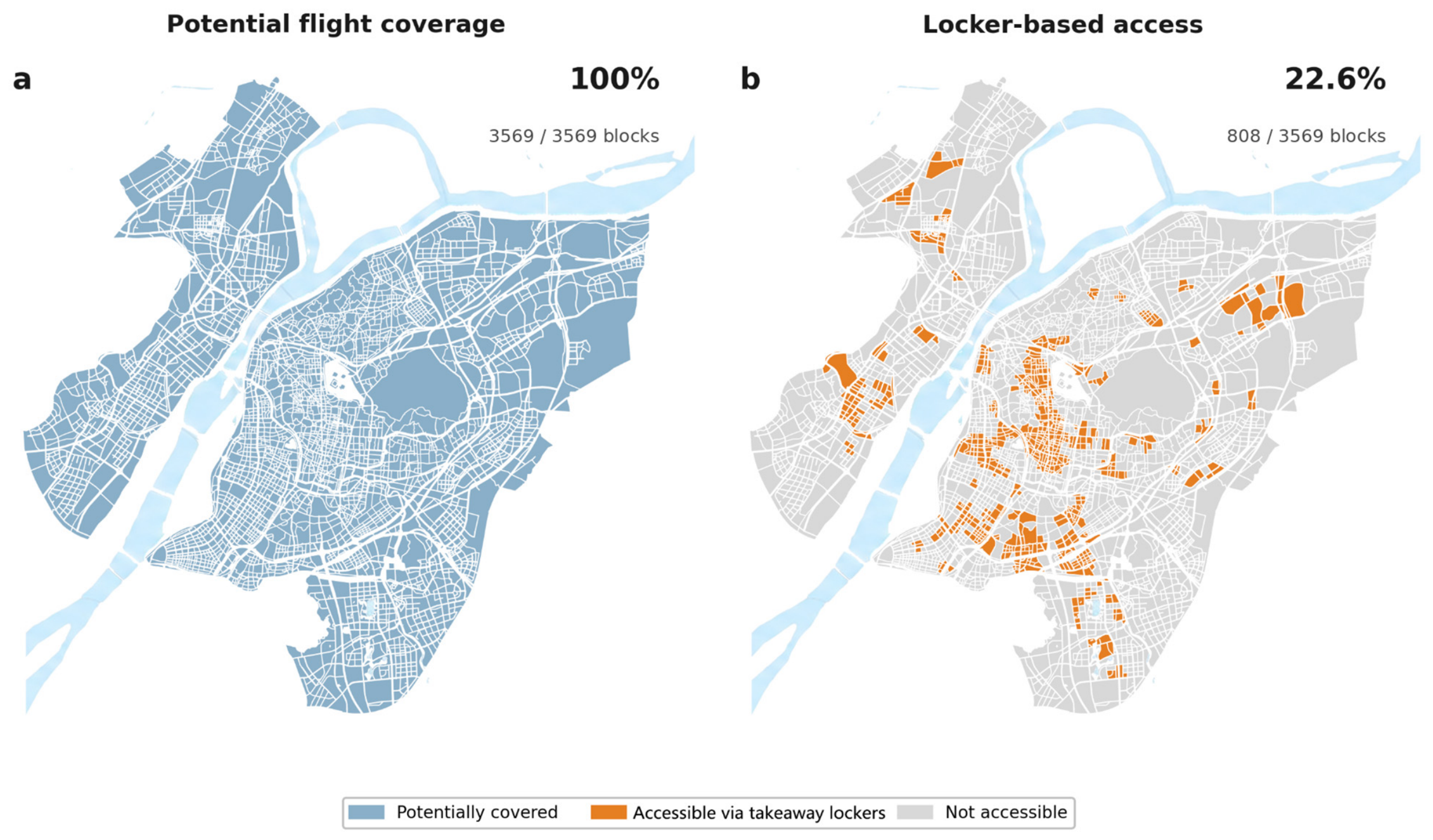
After the transition from road delivery to drone delivery, consumer demand enters the node network through pickup lockers. Under the baseline configuration, all 302 lockers connect to at least one launch node, forming 5034 node–locker edges, and the potential flight coverage includes all 3569 blocks. With the 417 m walking requirement, effective access is limited to 808 blocks (22.6%), covering 1,173,734 people (25.75% of the study-area population). These blocks can reach between one and nine lockers, with an average of 1.7 (Figure 3).
Figure 3.
Potential flight coverage and effective locker-based access under the baseline configuration.
Effective access is concentrated in blocks that satisfy the last-mile pickup condition, forming locally continuous or dispersed service areas according to the locker layout. Accessible demand is allocated through lockers to connected launch nodes and then shared among outlets, entering the outlet-relocation process.
3.3. Supply Redistribution After Baseline Network Introduction
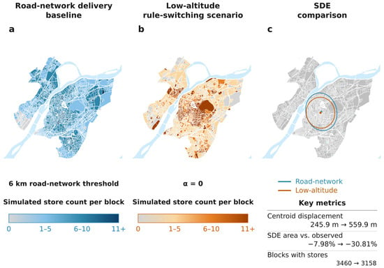
Under these demand-access and allocation conditions, outlets adjust their locations from the road-delivery baseline. In the seed-42 example, the SDE area decreases to 119.92 km2, a contraction of 24.81% relative to the road-delivery baseline, and blocks with outlets decrease from 3460 to 3158. Centroid displacement from the observed location is 559.9 m, compared with 245.9 m for the road baseline (Figure 4). Under this configuration, the spatial extent of the outlet distribution contracts and supply occupies fewer blocks. Across ten runs, mean SDE contraction is 25.03% (SD 0.48 percentage points), with 3122.8 ± 26.1 occupied blocks and 31.68 ± 0.30% of outlets within 1 km of nodes (Tables S2c and S3a).
Figure 4.
Outlet distributions under the road-delivery baseline and baseline drone-delivery scenario (seed 42). (a) Road-delivery baseline; (b) baseline drone-delivery scenario; and (c) SDE-area changes relative to the observed distribution. The drone-delivery scenario changes by −24.81% relative to the road-delivery baseline; all centroid displacements are relative to the observed centroid.
The locational relationship between outlets and launch nodes provides a reference for the subsequent impedance experiment. In the seed-42 baseline example, the outlet-weighted mean distance to the nearest node is 1774.4 m, and 31.93% of outlets lie within 1 km of nodes. Here, α = 0 corresponds to zero additional outlet–node distance impedances.
3.4. Outlet-Side Access Impedance and Node Proximity
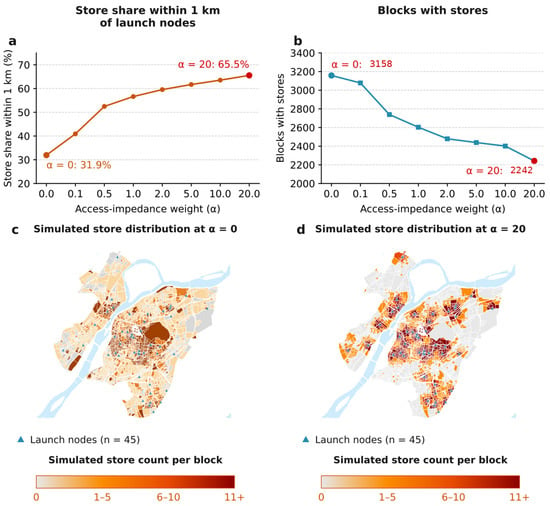
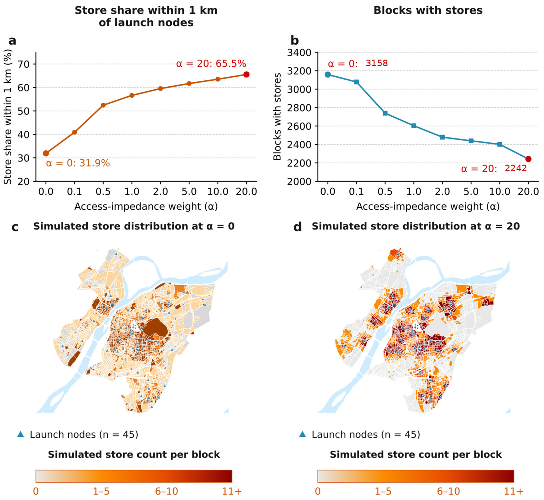
With infrastructure fixed, introducing outlet-side access impedance brings outlets closer to launch nodes. As α increases from zero to 20, the share of outlets within 1 km of nodes rises continuously from a mean of 31.68% to 65.07%, and mean blocks with outlets decrease from 3122.8 to 2244.7 (Table S3a). Figure 5 shows the seed-42 distributions and node-proximity example.
Figure 5.
Node proximity and outlet distributions under outlet-side access impedance (seed 42). (a) Share of outlets within 1 km of nodes; (b) number of blocks with outlets; and (c,d) simulated outlet distributions at α = 0 and α = 20.
As α increases, node proximity strengthens continuously, while SDE area follows a non-monotonic pattern of contraction followed by partial recovery. At α = 1, mean SDE contraction reaches 32.62% relative to the road-delivery baseline. At α = 20, mean contraction weakens to 29.73%. The two metrics therefore follow different trajectories; complete results are reported in Table S3a, including standard deviations and 95% confidence intervals.
3.5. Configuration-Dependent Spatial Responses
The preceding responses occur under a fixed facility layout. Varying one infrastructure condition at a time while holding the remaining parameters at baseline levels produces different changes in service access and supply distribution. Increasing flight-link distance from 5 to 20 km raises node–locker edges from 1689 to 11,209, reduces unconnected lockers from 16 to 0, and lowers the node-demand Gini coefficient from 0.5098 to 0.0950. Effective-access blocks increase only from 787 to 808, while the mean SDE-area response shifts from −43.81% to +1.50%. Changes in node connectivity and demand allocation can therefore correspond to substantial spatial supply responses even when consumer coverage changes only modestly. The realized-edge percentage rises from 12.43% to 82.48%, and the mean reachable-node percentage from 16.03% to 87.03% (Table S11). Under equal population allocation, this overlap makes node demand more similar; complete overlap would yield a Gini coefficient of zero.
Expanding walking radius mainly increases consumer access while producing limited change in overall supply form. Increasing the radius from 250 to 800 m raises effective-access blocks from 388 to 1557, or from 10.9% to 43.6% of all blocks. Mean SDE-area changes across the three radii are −24.86%, −25.03%, and −25.51%, respectively, while mean occupied blocks increase from 3012.1 to 3142.3 (Table S4e). Mean full major/minor axis lengths are 13.44/11.35, 12.89/11.81, and 12.89/11.73 km at 250, 417, and 800 m, respectively. Relative to matched 417 m runs, mean 1 km grid distribution differences are 15.14% at 250 m and 8.23% at 800 m. Removing any single block changes the corresponding ellipse area by less than 0.68% in every run (Table S4f), supporting a distinction between local redistribution and similar overall extent.
Walking-radius adjustments retain the locker layout, whereas changes in locker configuration alter both the location and scale of last-mile access. In the seed-42 example, moving from the reduced 151-locker configuration to the population-oriented 604-locker configuration increases effective-access blocks from 508 to 1620 and covered population from 571,553 to 3,952,934. Mean SDE-area changes for the 151-, 302-, and 604-locker scenarios are −26.40%, −25.03%, and −0.36%, respectively, with markedly weaker contraction under the expanded configuration (Table S2c). In the seed-42 example, centroid displacement from observations is 155.2 m with 604 lockers, compared with 1411.4 m with 151 lockers. These differences combine changes in locker quantity and location.
Returning lockers to the baseline layout and varying only launch-node configuration leaves consumer service coverage unchanged while altering outlet proximity. In the seed-42 example, increasing nodes from 23 to 60 reduces the mean nearest-node distance from 2863.2 to 1420.6 m and raises the share of outlets within 1 km from 18.12% to 34.49%. All three configurations serve 808 blocks and 1,173,734 people. With the 10 km flight threshold, each configuration connects all 302 lockers, so last-mile service coverage is jointly delimited by the fixed locker layout and walking radius. One-factor contrasts are reported in Table S4.
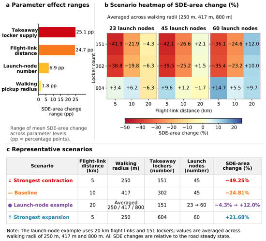
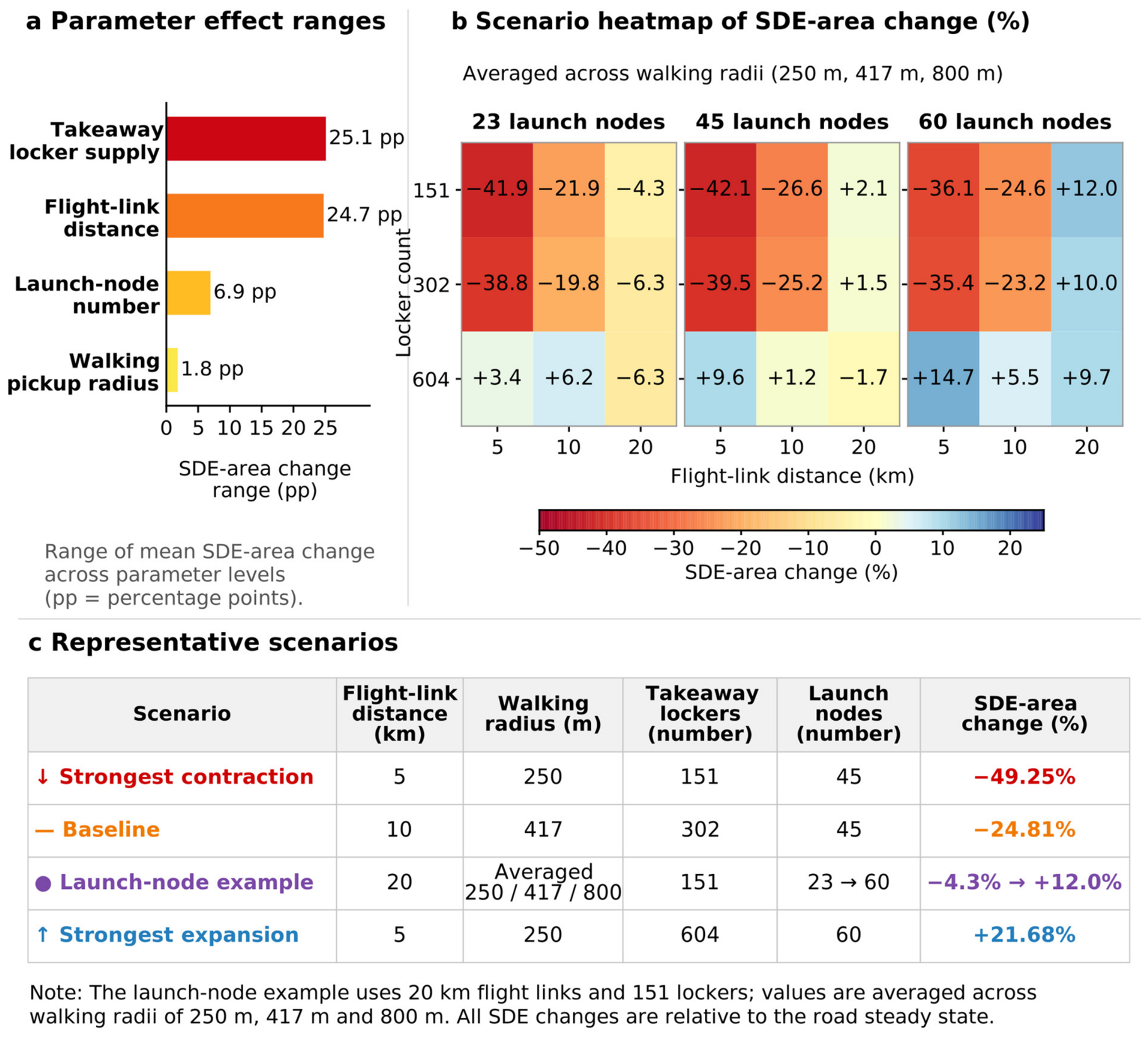
The one-factor comparisons show differentiated responses across infrastructure stages. Across all 81 facility combinations, mean SDE-area changes range from −46.69% to +21.62% (Table S2c); Figure 6 shows the seed-42 examples. In the seed-42 examples, the strongest contraction occurs with a 5 km flight-link distance, 250 m walking radius, 151 pickup lockers, and 45 launch nodes; the strongest expansion occurs under the same flight and walking conditions, with 604 lockers and 60 nodes. Based on the mean response at the three tested levels of each factor, the ten-run mean ranges of the SDE response are 25.93, 27.68, 8.54, and 2.40 percentage points for locker configuration, flight-link distance, launch-node configuration, and walking radius, respectively. The tested combinations span both contraction and expansion, with larger differences in mean response associated with locker configuration and flight-link distance. Flight distance and locker configuration rank in the top two in every run, ranking as first six and four times, respectively; their paired comparison produces p = 0.1814 (Table S10).
Figure 6.
Facility combinations and SDE-area responses (seed 42). (a) Range of mean response across the tested levels of each factor, in percentage points; (b) combination responses averaged across the three walking radii; and (c) strongest contraction, baseline, launch-node example, and strongest expansion scenarios. All area changes are relative to the road-delivery baseline.
4. Discussion
4.1. Node Access and Spatial Redistribution of Food-Delivery Supply
Under the baseline scenario, the spatial extent of the outlet distribution contracts after introduction of the drone-delivery network; adding outlet-side distance impedance further increases the share of outlets around launch nodes. These results reflect two connected processes. First, consumer demand is aggregated through pickup lockers to launch nodes able to provide service, and an outlet’s node assignment affects the demand it can share. Second, distance impedance increases the locational disadvantage of outlets farther from nodes and strengthens the relative attractiveness of nearby locations. Node service connections and outlet access conditions therefore jointly contribute to simulated supply redistribution. Replacing equal allocations among nodes with allocations weighted by attached outlet counts changes the mean contraction at α = 0 from 25.03% to 48.73%, while node-proximity shares still rise as α increases (Table S8). Supply responses therefore depend jointly on service connections and demand allocations.
These results relate to the physical locational relationships emphasized in platform-food-service research. Talamini et al. [1] examined the spatial organization of platformized food services, while Hu et al. [3] identified links among commercial centers, consumer demand, and outlet micro-locations in Xinjiekou. The new delivery network further changes how outlets access demand: outlets can reach more distant demand through aerial connections while entering the network through specific ground nodes. Launch nodes thus become a new spatial condition influencing outlet-location relationships. Because the baseline nodes are selected from commercial centers and complexes, the simulated responses also incorporate existing commercial centrality together with the influence of the added network. Holding the node count at 45, random populated-block layouts and layouts more than 1 km from the original commercial nodes yield mean contractions of 18.94% and 13.50%, while increasing α from zero to 20 raises nearby outlet shares from 28.45% to 63.17% and from 25.00% to 58.43%, respectively (Table S7).
Node-local concentration and city-scale spatial extent follow different trajectories. As α increases, node proximity strengthens continuously, while SDE area reaches its minimum at α = 1 and then generally recovers. Outlets can move closer to nodes distributed across different districts while maintaining a relatively broad city-scale extent. SDE, node proximity, and the number of blocks with outlets therefore provide complementary descriptions of supply reorganization within and between node service areas.
4.2. Differences Between Effective Access and Supply Response
The baseline network produces 100% potential flight coverage but only 22.6% effective access, revealing a substantial spatial gap between the two measures. Food-delivery research has linked service use and food access to built-environment conditions and online and offline accessibility [31,43]. Pickup-facility research has also examined facility layout, service coverage, and spatial equity [44,45]. In the modeled system, flight links, locker layout, and walking conditions jointly determine whether consumers can enter the service network.
The growth in effective access and changes in supply form occur at different magnitudes. A larger walking radius substantially increases the accessible population while producing little change in SDE area; a longer flight-link distance adds relatively few accessible blocks but shifts the supply response from marked contraction to slight expansion. In the model, the flight-link distance also changes the set of nodes that can serve a given consumer and therefore redistributes demand among nodes. The demand received by individual nodes and the allocation of outlets among them are more directly connected to outlet relocation, which is why service access and supply response are reported separately.
He et al. [14] showed associations between the spatial distribution of Hangzhou’s UAV logistics network and its urban spatial conditions, while Wang et al. [15] extended the discussion to urban morphology and network costs through cross-city simulations. This study further examines the relationship between changes in facility connections and supply distribution within a fixed urban setting. Flight links, last-mile access, and outlet–node proximity operate at different stages of the service chain, so the resulting spatial response is best described using multiple complementary indicators.
4.3. Implications for Infrastructure Comparison
Both contraction and expansion occur across the 81 configurations, indicating that infrastructure alternatives should be compared as combinations rather than isolated components. This pattern is consistent with drone last-mile research emphasizing interactions among technology, routing, facilities, and operational decisions [6,12,13]. The 604-locker scenario follows a population-oriented expansion rule, so its results jointly reflect changes in facility quantity and location. Last-mile logistics research has likewise examined pickup-facility efficiency and location decisions [46,47]. In the Nanjing scenarios, population-oriented expansion serves more consumers and reduces the contraction of supply extent. The result supports comparison of alternative infill strategies, while the optimal number and placement of lockers would require additional facility-location optimization and operational constraints.
Spatial gaps can be screened along the delivery path. In areas with weak flight connectivity, node–locker edges and node-demand distributions can be compared. In areas with flight coverage but limited last-mile access, population and walking conditions can inform comparison of additional locker locations. Where outlet-to-node distances are long, launch-node layouts warrant further evaluation. Under baseline conditions, additional launch nodes improve outlet proximity while leaving consumer service coverage unchanged, illustrating that expansion objectives differ across infrastructure stages.
The spatial metrics developed here are suited to pre-implementation screening of infrastructure alternatives. Engineering and implementation stages should additionally examine UAV payload and endurance, fleet and node capacities, charging or battery swapping, order scheduling, airspace safety, noise, weather, service reliability, and operating costs [12,13]. Together, these factors determine whether spatially favorable configurations can be translated into operational drone systems and stable service levels. Alternative configurations should therefore be evaluated jointly in terms of spatial supply response, accessibility objectives, operational constraints, and community impacts. The operating scenarios illustrate this dependence. With a charge-to-flight-time ratio of one, the 10 km network has mean SDE-area changes of −11.92% and −24.27% with five and twenty drones per node, respectively, compared to −25.03% with the core model. At 20 km, twenty drones per node with a 30 min full-flight budget yield −33.80%; extending that budget to 60 min yields produces −1.65% compared to +1.50% with the core model (Table S13). The baseline network therefore retains contraction under the tested operating conditions, with a magnitude that depends on fleet capacity; responses at longer flight thresholds also depend on round-trip endurance. SDE contraction describes supply extent; consumer access and operational performance provide separate evaluation criteria.
4.4. Limitations and Future Research
The scenarios use existing urban data, proxy launch nodes and lockers, and predefined rules for facility reduction and expansion. The road-delivery baseline has low block-level correlation with the observed distribution and substantially more blocks with outlets; its interpretation is therefore focused on providing a common reference for drone-delivery scenarios and on comparing broad spatial morphology, while specific block counts are treated as model-state records rather than block-level predictions. Ten repetitions of the full initialization–road–low-altitude sequence yield a mean contraction of 25.14%; across seven relocation, exploration, and decay settings, the mean contraction ranges from 24.53% to 25.58%, with larger variation in occupied blocks (Supplementary Method S2 and Table S9). Outcomes obtained under the predefined stopping criterion support comparisons of broad spatial form and relative alternatives under the present assumptions; observed outlet relocation and operating data would support behavioral calibration. The observed-start controls in Section 3.1 retain overall contraction but reduce its magnitude and reverse the occupancy change, so both the reference distribution and outcome metric are specified when interpreting results.
Population is used as a proxy for consumer demand, the citywide outlet total is fixed, and outlet benefits and location choices are represented with simplified rules. Future extensions can incorporate rents, business-type differences, platform rankings, and consumer preferences; the outlet-side impedance parameter can also be behaviorally calibrated using observed operating and relocation data. Fleet sizes and order intensities define comparative operating conditions (Supplementary Method S3). Weather and no-fly restrictions remain relevant to finer-scale engineering designs. Future work can use pilot-order records, service durations, and outlet operating data to calibrate demand allocation and node-access processes, and can test transferability through cross-city comparisons under different population, commercial, and facility distributions.
5. Conclusions
Using central Nanjing as a case study, this research links effective consumer access, node-level demand allocation, and outlet relocation to examine spatial supply responses after the introduction of an urban drone-delivery network. Under the baseline scenario, the potential flight coverage includes all blocks, while only 22.6% have effective access; the SDE area of the outlet distribution contracts by a mean of 25.03% across ten runs relative to the road-delivery baseline. As outlet-side access impedance increases, outlets move progressively closer to launch nodes, while the city-scale SDE extent changes non-monotonically. Observed-start and allocation controls retain their contraction under baseline infrastructure while the magnitude depends on these settings.
Infrastructure combinations produce mean SDE-area changes ranging from −46.69% to +21.62%, showing that the spatial supply response to urban drone delivery depends on configuration. Flight links and the locker layout alter the demand available to nodes, walking conditions directly affect consumer access, and launch-node configuration affects outlet access distances. Pre-implementation spatial assessment should follow the complete service path and jointly compare effective service coverage, node organization, and supply distribution, treating flight coverage and individual facility counts as component indicators within an integrated evaluation.
Supplementary Materials
The following supporting information can be downloaded at: https://www.mdpi.com/article/10.3390/drones10110854/s1, covering outputs for the 81 infrastructure configurations and the outlet-side access-impedance experiment, together with a reproducibility archive containing the analysis code, processed inputs, input hashes, and execution instructions. The Supplementary Materials include: Supplementary Methods: Supplementary Method S1. Model Definitions and Updating; Supplementary Method S2. Control Designs and Statistics; Supplementary Method S3. Operational Scenarios. Supplementary Figure: Figure S1. Model diagnostics for observed food-delivery supply. Supplementary Tables: Table S1. Data sources, processing, and scenario uses. Table S2a. Infrastructure configurations and network indicators (seed 42). Table S2b. Spatial supply indicators for infrastructure configurations (seed 42). Table S2c. Summary statistics across replicates for 81 configurations (ten runs each; mean ± sample SD). Table S3a. Summary statistics across replicates for outlet-side access impedance (ten runs per α). Table S3b. Spatial indicators for access-impedance examples (seed 42). Table S4a. Single-factor flight-distance examples (seed 42). Table S4b. Single-factor walking-radius examples (seed 42). Table S4c. Single-factor locker-configuration examples (seed 42). Table S4d. Single-factor launch-node examples (seed 42). Table S4e. Indicators from repeated walking-radius simulations (ten runs per level). Table S4f. Local distribution differences and single-block influence in walking scenarios (ten runs per level). Table S5. Rationale and interpretation of main parameters and indicators. Table S6. Observed-start controls under baseline infrastructure. Table S7. Node-layout controls (ten runs per setting). Table S8. Demand-allocation controls (ten runs per rule and α level). Table S9. Sensitivity to relocation, exploration, and probability decay (ten runs per setting). Table S10. Summary statistics across replicates for infrastructure-factor response ranges. Table S11. Connection overlap and node-demand allocation by flight distance. Table S12. Definitions and comparison conventions for auxiliary network indicators. Table S13a. Operational conditions and spatial responses at 10 km (ten runs; mean ± sample SD). Table S13b. Flight-distance and endurance comparisons at α = 0 (ten runs; mean ± sample SD).
Author Contributions
Conceptualization, K.Z.; methodology, K.Z.; software, K.Z.; formal analysis, K.Z.; visualization, K.Z.; writing—original draft preparation, K.Z.; data curation, K.Z., W.Z. and X.Z.; supervision, Y.S.; writing—review and editing, X.H. and P.Y. All authors have read and agreed to the published version of the manuscript.
Funding
This research was funded by the National Natural Science Foundation of China (grant number 52378048); the China Postdoctoral Science Foundation (grant number 2025M780749); and the Project of Philosophy and Social Science Research in Colleges and Universities of Jiangsu Province (grant number 2024SJYB0140).
Institutional Review Board Statement
This study did not involve human participants or animal experiments; therefore, an institutional ethics review was not required.
Informed Consent Statement
This study did not involve human participants; therefore, informed consent was not required or applicable.
Data Availability Statement
Scenario-level results supporting the study’s findings are included in the Supplementary Materials, with the data sources and preprocessing procedures described in Table S1. The analysis code and shareable processed inputs required to reproduce the reported analyses are provided in the supplementary reproducibility archive. Raw third-party source data are not redistributed beyond the processed inputs included with the submission.
Acknowledgments
During the preparation of this manuscript, the authors used ChatGPT (GPT-5.6, OpenAI, San Francisco, CA, USA) to assist with translation and language editing. The authors reviewed and revised the resulting text as needed and take full responsibility for the content of the manuscript.
Conflicts of Interest
The authors declare no conflicts of interest.
References
- Talamini, G.; Li, W.; Li, X. From brick-and-mortar to location-less restaurant: The spatial fixing of on-demand food delivery platformization. Cities 2022, 128, 103820. [Google Scholar] [CrossRef] [Scilit]
- Azzoni, C.R.; Moita, R.M.S.; Rodrigues, M. Meal delivery and the local restaurant industry. Appl. Geogr. 2025, 176, 103524. [Google Scholar] [CrossRef] [Scilit]
- Hu, X.; Zhang, G.; Shi, Y.; Yu, P. How information and communications technology affects the micro-location choices of stores on on-demand food delivery platforms: Evidence from Xinjiekou’s central business district in Nanjing. ISPRS Int. J. Geo-Inf. 2024, 13, 44. [Google Scholar] [CrossRef] [Scilit]
- Wing. Australia’s First Store-to-Door Drone Delivery Service Launches with Coles. 2022. Available online: https://wing.com/news/australias-first-store-to-door-drone (accessed on 4 July 2026).
- Wing. Wing and Walmart Announce World’s Largest Drone Delivery Expansion. 2025. Available online: https://wing.com/news/wing-and-walmart-announce-world-s-largest-drone-delivery-expansion-ever (accessed on 4 July 2026).
- Hu, Z.-H.; Huang, Y.-L.; Li, Y.-N.; Bao, X.-Q. Drone-Based Instant Delivery Hub-and-Spoke Network Optimization. Drones 2024, 8, 247. [Google Scholar] [CrossRef] [Scilit]
- Zou, B.; Wu, S.; Gong, Y.; Yuan, Z.; Shi, Y. Delivery network design of a locker-drone delivery system. Int. J. Prod. Res. 2024, 62, 4097–4121. [Google Scholar] [CrossRef] [Scilit]
- Zhu, W.; Hu, X.; Pei, J.; Pardalos, P.M. Minimizing the total travel distance for the locker-based drone delivery: A branch-and-cut-based method. Transp. Res. Part B Methodol. 2024, 184, 102950. [Google Scholar] [CrossRef] [Scilit]
- Meituan. 2021 Corporate Social Responsibility Report. 2022. Available online: https://www.meituan.com/csr/report (accessed on 20 October 2026). (In Chinese)
- Murray, C.C.; Chu, A.G. The flying sidekick traveling salesman problem: Optimization of drone-assisted parcel delivery. Transp. Res. Part C Emerg. Technol. 2015, 54, 86–109. [Google Scholar] [CrossRef] [Scilit]
- Agatz, N.; Bouman, P.; Schmidt, M. Optimization approaches for the traveling salesman problem with drone. Transp. Sci. 2018, 52, 965–981. [Google Scholar] [CrossRef] [Scilit]
- Eskandaripour, H.; Boldsaikhan, E. Last-mile drone delivery: Past, present, and future. Drones 2023, 7, 77. [Google Scholar] [CrossRef] [Scilit]
- Shuaibu, A.S.; Mahmoud, A.S.; Sheltami, T.R. A review of last-mile delivery optimization: Strategies, technologies, drone integration, and future trends. Drones 2025, 9, 158. [Google Scholar] [CrossRef] [Scilit]
- He, H.; Ye, H.; Xu, C.; Liao, X. Exploring the spatial heterogeneity and driving factors of UAV logistics network: Case study of Hangzhou, China. ISPRS Int. J. Geo-Inf. 2022, 11, 419. [Google Scholar] [CrossRef] [Scilit]
- Wang, W.; Teng, Z.; Guo, Z.; He, J. How urban morphology is associated with simulated drone logistics network costs: Location simulation evidence from 101 Chinese cities. ISPRS Int. J. Geo-Inf. 2026, 15, 249. [Google Scholar] [CrossRef] [Scilit]
- Straubinger, A.; de Groot, H.L.F.; Verhoef, E.T. E-commerce, delivery drones and their impact on cities. Transp. Res. Part A Policy Pract. 2023, 178, 103841. [Google Scholar] [CrossRef] [Scilit]
- He, Z.; Han, G.; Cheng, T.C.E.; Fan, B.; Dong, J. Evolutionary food quality and location strategies for restaurants in competitive online-to-offline food ordering and delivery markets: An agent-based approach. Int. J. Prod. Econ. 2019, 215, 61–72. [Google Scholar] [CrossRef] [Scilit]
- Hansen, W.G. How accessibility shapes land use. J. Am. Inst. Plan. 1959, 25, 73–76. [Google Scholar] [CrossRef] [Scilit]
- Geurs, K.T.; van Wee, B. Accessibility evaluation of land-use and transport strategies: Review and research directions. J. Transp. Geogr. 2004, 12, 127–140. [Google Scholar] [CrossRef] [Scilit]
- Keeble, M.; Adams, J.; Bishop, T.R.P.; Burgoine, T. Socioeconomic inequalities in food outlet access through an online food delivery service in England: A cross-sectional descriptive analysis. Appl. Geogr. 2021, 133, 102498. [Google Scholar] [CrossRef] [Scilit]
- Huang, Z.; Guo, Y.; Zhao, M. Digital food delivery platforms and the spatial inequality of urban food access. Appl. Geogr. 2026, 193, 104096. [Google Scholar] [CrossRef] [Scilit]
- Sakai, T.; Alho, A.R.; Bhavathrathan, B.K.; Chiara, G.D.; Gopalakrishnan, R.; Jing, P.; Hyodo, T.; Cheah, L.; Ben-Akiva, M. SimMobility Freight: An agent-based urban freight simulator for evaluating logistics solutions. Transp. Res. Part E Logist. Transp. Rev. 2020, 141, 102017. [Google Scholar] [CrossRef] [Scilit]
- van Heeswijk, W.J.A.; Mes, M.R.K.; Schutten, J.M.J.; Zijm, W.H.M. Evaluating urban logistics schemes using agent-based simulation. Transp. Sci. 2020, 54, 651–675. [Google Scholar] [CrossRef] [Scilit]
- Nanjing Municipal Bureau of Planning and Natural Resources. Nanjing Territorial Spatial Master Plan (2021–2035). 2024. Available online: https://ghj.nanjing.gov.cn/ghbz/ztgh/202410/t20241024_4992742.html (accessed on 4 July 2026). (In Chinese)
- Zhang, S.; Luan, H.; Zhen, F.; Kong, Y.; Xi, G. Does online food delivery improve the equity of food accessibility? A case study of Nanjing, China. J. Transp. Geogr. 2023, 107, 103516. [Google Scholar] [CrossRef] [Scilit]
- Cragg, J.G. Some statistical models for limited dependent variables with application to the demand for durable goods. Econometrica 1971, 39, 829–844. [Google Scholar] [CrossRef] [Scilit]
- Mullahy, J. Specification and testing of some modified count data models. J. Econom. 1986, 33, 341–365. [Google Scholar] [CrossRef] [Scilit]
- Breiman, L. Random forests. Mach. Learn. 2001, 45, 5–32. [Google Scholar] [CrossRef] [Scilit]
- Yildiz, B.; Savelsbergh, M. Provably high-quality solutions for the meal delivery routing problem. Transp. Sci. 2019, 53, 1372–1388. [Google Scholar] [CrossRef] [Scilit]
- Zhang, Z.; Liu, C. Exploration of riding behaviors of food delivery riders: A naturalistic cycling study in Changsha, China. Sustainability 2023, 15, 16227. [Google Scholar] [CrossRef] [Scilit]
- Wang, Z.; He, S.Y. Impacts of food accessibility and built environment on on-demand food delivery usage. Transp. Res. Part D Transp. Environ. 2021, 100, 103017. [Google Scholar] [CrossRef] [Scilit]
- Liu, B.; Zhou, K.; Lei, A.; Wang, Y.; Wang, L. Exploring factors influencing online food consumption using multi-source data: A case study of Hongkou District, Shanghai. Urban Plan. Int. 2024, 39, 27–35. (In Chinese) [Google Scholar] [CrossRef]
- Yang, H.; Wu, J.; Zhang, Z.; Liu, X.; D’Ariano, A. Optimal design for an urban truck-drone collaborative delivery system enhanced with relay points. Transp. Res. Part E Logist. Transp. Rev. 2025, 204, 104425. [Google Scholar] [CrossRef] [Scilit]
- Meituan. Meituan UAV Releases Its Fourth-Generation Aircraft and Presents a New Urban Low-Altitude Logistics Solution at 2023 WAIC. 2023. Available online: https://www.meituan.com/news/NN230706019014042 (accessed on 9 September 2026). (In Chinese)
- Woodworth, A. Customer Demand and Wing’s Aircraft Library Design Approach Shape New Aircraft. 2024. Available online: https://wing.com/news/customer-demand-and-wings-aircraft (accessed on 9 September 2026).
- Zipline. Zipline Unveils Autonomous System for Quiet, Fast, and Precise Home Delivery. 2023. Available online: https://www.zipline.com/newsroom/zipline-unveils-new-autonomous-system-capable-of-quiet-fast-and-precise-home-delivery (accessed on 9 September 2026).
- Meituan. Meituan–INFORMS TSL Research Challenge: Order Data and Clarification. 2024. Available online: https://github.com/meituan/Meituan-INFORMS-TSL-Research-Challenge (accessed on 23 October 2026).
- Ko, Y.K.; Han, H.; Oh, Y.; Ko, Y.D. The development of an optimal operation algorithm for food delivery using drones considering time interval between deliveries. Drones 2024, 8, 230. [Google Scholar] [CrossRef] [Scilit]
- Es Yurek, E. Impact of drone battery recharging policy on overall carbon emissions: The traveling salesman problem with drone. Drones 2024, 8, 108. [Google Scholar] [CrossRef] [Scilit]
- Gini, C. Variabilità e Mutabilità: Contributo allo Studio delle Distribuzioni e delle Relazioni Statistiche; Tipografia di Paolo Cuppini: Bologna, Italy, 1912. [Google Scholar]
- Yuill, R.S. The standard deviational ellipse: An updated tool for spatial description. Geogr. Ann. Ser. B Hum. Geogr. 1971, 53, 28–39. [Google Scholar] [CrossRef]
- Spearman, C. The proof and measurement of association between two things. Am. J. Psychol. 1904, 15, 72–101. [Google Scholar] [CrossRef] [Scilit]
- Li, L.; Feng, R.; Xi, J.; Wang, F. Spatial drivers and effects of urban food accessibility: Comparison of conventional and online-to-offline services. Appl. Geogr. 2023, 152, 102894. [Google Scholar] [CrossRef] [Scilit]
- Morganti, E.; Dablanc, L.; Fortin, F. Final deliveries for online shopping: The deployment of pickup point networks in urban and suburban areas. Res. Transp. Bus. Manag. 2014, 11, 23–31. [Google Scholar] [CrossRef] [Scilit]
- Schaefer, J.S.; Figliozzi, M.A. Spatial accessibility and equity analysis of Amazon parcel lockers facilities. J. Transp. Geogr. 2021, 97, 103212. [Google Scholar] [CrossRef] [Scilit]
- Iwan, S.; Kijewska, K.; Lemke, J. Analysis of parcel lockers’ efficiency as the last mile delivery solution: The results of the research in Poland. Transp. Res. Procedia 2016, 12, 644–655. [Google Scholar] [CrossRef] [Scilit]
- Kahr, M. Determining locations and layouts for parcel lockers to support supply chain viability at the last mile. Omega 2022, 113, 102721. [Google Scholar] [CrossRef] [Scilit]

Disclaimer/Publisher’s Note: The statements, opinions and data contained in all publications are solely those of the individual author(s) and contributor(s) and not of MDPI and/or the editor(s). MDPI and/or the editor(s) disclaim responsibility for any injury to people or property resulting from any ideas, methods, instructions or products referred to in the content. |
© 2026 by the authors. Licensee MDPI, Basel, Switzerland. This article is an open access article distributed under the terms and conditions of the Creative Commons Attribution (CC BY) license.