Aerodynamic Performance of a Hand-Launched Biplane UAV with Distributed Electric Propulsion

Highlights

What are the main findings?

• Under comparable design constraints, simulations predict higher lift per unit shaft power and smaller nose-down moments about the respective layout-selected reference centers of gravity for the propeller-aided biplane than for the conventional leading-edge tractor configuration over the representative hand-launch angle-of-attack range.
• A smaller propeller-induced airframe drag penalty largely offsets the biplane’s clean-airframe disadvantage, with comparable shaft-power levels at the sampled fixed-rpm cruise conditions.

What are the implications of the main findings?

• Full-aircraft assessments should consider lift and forward force per unit shaft power alongside pitching moments and cruise performance, and propeller efficiency alone cannot capture configuration benefits.
• The sensitivity of predicted airframe loads supports using unsteady propeller simulations with transition modeling to assess the aerodynamic performance of the present UAV.

Abstract

Hand-launched unmanned aerial vehicles require adequate low-speed lift and cruise efficiency. This study investigates a 3 kg propeller-aided biplane (PAB) with distributed electric propulsion using unsteady computational fluid dynamics. Propeller–wing arrangements are examined, followed by complete-aircraft simulations with transition modeling and sliding meshes. A conventional tractor configuration (CONV) provides a reference under comparable design constraints. Among the arrangements examined, over-the-wing and leading-edge tractor installations provide substantial lift augmentation. Predicted airframe loads are sensitive to transition modeling and the representation of propeller rotation. Although PAB has a lower clean-airframe lift-to-drag ratio, its smaller propeller-induced airframe drag penalty largely offsets this disadvantage at sampled fixed-rpm cruise conditions. At the 5 m/s hand-launch condition and angles of attack of 8–12°, PAB provides greater lift per unit shaft power with a comparable positive net forward force. At 12°, the lift-per-power gain is approximately 4%. About the respective design reference centers of gravity, cycle-mean nose-down moment magnitudes are approximately 77% and 49% smaller for PAB than for CONV at 8° and 12°. These predictions indicate hand-launch benefits for this non-optimized configuration pair under the prescribed conditions.

1. Introduction

The low-altitude economy has increased interest in unmanned aerial vehicles (UAVs) for environmental monitoring, infrastructure inspection, agriculture, and emergency services [1]. Small fixed-wing UAVs offer sustained coverage, while hand launch reduces dependence on ground infrastructure. Long-endurance hand-launched solar-powered aircraft combine aerodynamic efficiency with operational portability [2]. However, low launch speeds limit available lift, and sufficient forward force is needed to accelerate after release. Short wing chords and low speeds also lead to low Reynolds numbers, at which transition and laminar separation can strongly influence performance [3]. Therefore, hand-launched UAVs must balance low-speed lift and forward force against power consumption, pitching moment requirements, and cruise efficiency.

Distributed electric propulsion (DEP) allows propellers to be positioned in conjunction with lifting surfaces to address these requirements [4]. Leading-edge propellers can enhance low-speed lift through slipstream acceleration. The NASA SCEPTOR demonstrator design combined distributed high-lift propellers with wingtip-mounted cruise propellers to accommodate both flight regimes [5]. Keller [6] showed that more propellers do not necessarily improve cruise efficiency; benefits depend on installation, thrust allocation, and the wing-sizing potential from enhanced low-speed lift.

Propeller placement alters both wing loading and propeller inflow. Using a panel/viscous vortex particle hybrid method, Wang et al. [7] demonstrated lift and drag responses to streamwise, spanwise, and vertical placement, identifying over-the-wing installations that combined lift enhancement with reduced wing drag under selected conditions. Sinnige et al. [8] showed that suitably rotating wingtip propellers can reduce induced drag. However, component-level improvements do not necessarily translate into overall benefits. Cole et al. [9] emphasized the evaluation of installation choices using a consistent coupled-system metric, and de Vries and Vos [10] showed that over-the-wing aerodynamic benefits must be considered together with installed propeller efficiency and powertrain characteristics.

These interactions are not limited to changes in local dynamic pressure. Ananda et al. [11] showed that tractor-propeller slipstreams modify transition and separation on a low-Reynolds-number wing. For an over-the-wing installation, de Vries et al. [12] identified adverse boundary layer responses associated with slipstream contraction and blade-induced pressure disturbances, depending on installation geometry and operating conditions. Experiments by Okawa et al. [13] revealed vortex formation and shedding synchronized with propeller rotation.

Biplanes accommodate lifting area within a restricted span but introduce interactions governed by wing spacing, stagger, and relative incidence [14]. Experiments by Jones et al. [15] showed performance penalties relative to a single wing at small angles of attack, whereas selected arrangements provided lift gains at larger angles. Their aerodynamic value depends on configuration-specific interactions rather than simply distributing the lifting area between two wings.

Combining biplanes with propellers offers complementary interaction mechanisms. Wang et al. [16] investigated a double-wing configuration exploiting upstream propeller-induced suction over one wing and accelerated downstream flow over the other, demonstrating improved wing-assembly performance. Wang and Zhou [17] analyzed a hand-launched flying-wing UAV with an adjustable upper wing using transition modeling and a quasi-steady propeller treatment, including cruise performance and launch accelerations. More recently, Wang et al. [18] proposed a complete propeller-induced lift-enhancing vertical take-off and landing aircraft concept, while their numerical analysis used a representative wing segment to examine propeller inclination and upper-wing incidence. These studies provide a basis for evaluating propeller-aided biplanes in different operating modes.

The biplane considered here must balance low-speed lift enhancement against cruise efficiency using the same wing–propeller arrangement. This balance requires assessing shaft power, net forward force, and pitching moment about the aircraft center of gravity.

This study investigates a 3 kg hand-launched UAV with a propeller-aided biplane (PAB) configuration and four distributed electric propellers. The propeller disks lie above the lower wing and upstream of the upper wing to exploit upstream induction and downstream slipstream acceleration, respectively. Representative arrangements are first examined using a periodic model, followed by complete-aircraft analysis. A conventional tractor DEP configuration (CONV) provides a reference under common mission requirements, identical propulsion system power limits, and comparable total wing areas and spans. This comparison combines sliding-mesh simulations and transition modeling to assess complete-aircraft forces, pitching moments about the design reference centers of gravity, and shaft power at prescribed hand-launch and cruise conditions. Section 2, Section 3, Section 4 and Section 5 present the numerical methods and validation, propeller–wing interactions, complete-aircraft results, and conclusions, respectively.

2. Numerical Method

2.1. CFD Method

The numerical simulations are performed using ANSYS Fluent 2021R1 in this study. The Reynolds-averaged Navier–Stokes equations are discretized using a cell-centered finite-volume method. Air is treated as an ideal gas. The convective fluxes are computed using the Roe flux difference splitting scheme with second-order spatial accuracy.

The sliding-mesh method (SMM) resolves propeller–airframe aerodynamic interactions. The domain comprises a stationary zone and multiple rotating zones, with propeller rotation represented by rigid-body mesh motion. Sliding interfaces exchange information between stationary and rotating domains.

Unsteady simulations use implicit dual-time stepping with second-order temporal discretization. The initial flow field of the propeller is obtained from a multiple reference frame (MRF) solution which is based on the quasi-steady assumption. For propeller simulations, the time step corresponds to 1° of rotation with 20 inner iterations. Within-step convergence is assessed jointly from residual reduction and stabilization of the integrated forces and moments. A residual reduction of approximately two to three orders of magnitude and relative changes in the monitored loads below 10⁻³ between successive iterations over the final five inner iterations are used as practical indicators. Periodic stabilization is assessed from repeatable load histories and stable successive cycle means over a complete propeller revolution. Cycle averages use the final stabilized revolution; quantitative checks are given in Section 4.1.3.

Turbulence is modeled using the Shear Stress Transport (SST) model or the k-k_L-ω transition model according to the Reynolds number and the objective of the analysis. Details of the k-k_L-ω transition model can be found in Ref. [19]. The far-field turbulence intensity is set to 0.5%; for the k-k_L-ω model, the laminar kinetic energy is set to 10⁻⁶ m²/s² and the turbulent-viscosity ratio to 2.

2.2. Validations

To validate the present numerical method, simulations were performed for three representative test cases: an airfoil, a biplane configuration, and a propeller.

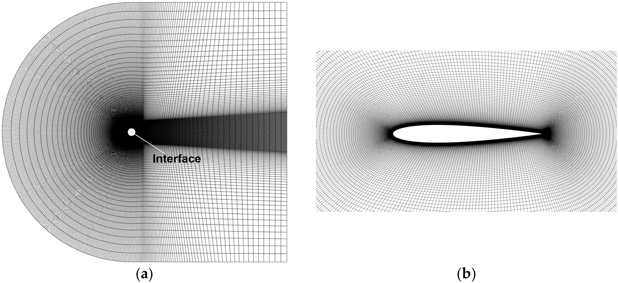
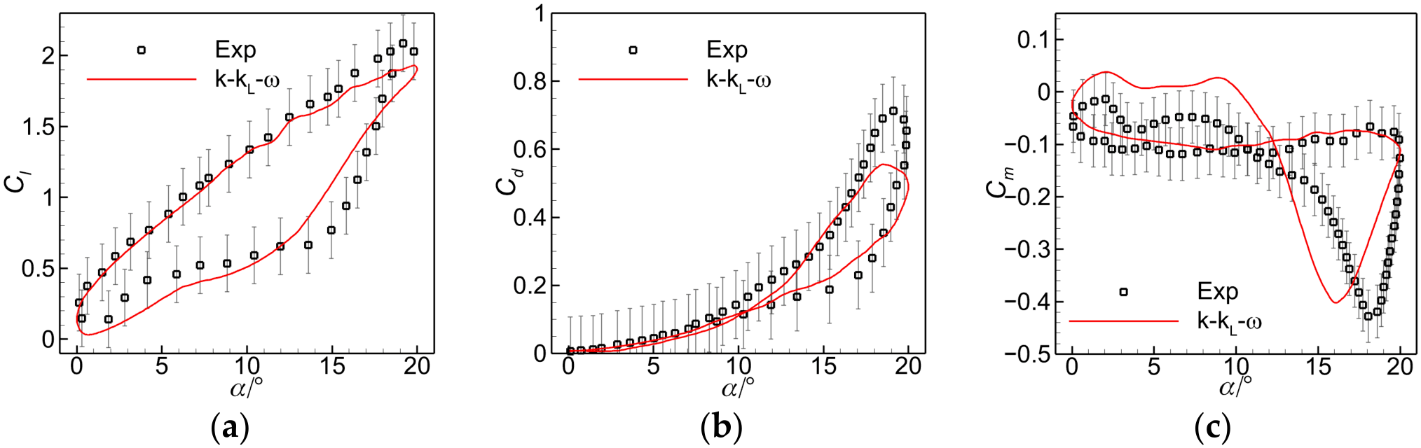
The first validation case was the pitching oscillation of the NACA0012 airfoil. The Mach number and the Reynolds number are M = 0.035 and Re = 4.86 × 10⁵, respectively. The pitching motion is given by α = α₀ + α₁sin (2πft), where α₀ = 10°, α₁ = 10° and f = 1.62 Hz. The reduced frequency is k = 0.253. The pitching axis is located at the quarter-chord position. The mesh is shown in Figure 1, consisting of approximately 1.6 × 10⁵ cells. Each oscillation cycle is discretized into 1000 time steps. Figure 2 compares the numerical and experimental results [20]. Considering the experimental uncertainties, which increase as free-stream velocity decreases [21], the calculations capture the overall lift, drag, and pitching moment trends. Discrepancies remain during dynamic stall, where the unsteady coupling of transition, separation, and reattachment is difficult to resolve. This initial validation indicates that the k-k_L-ω model can reasonably capture the main aerodynamic characteristics at low-to-moderate Reynolds numbers.

Figure 1. Computational mesh for the pitching oscillation of the NACA0012 airfoil: (a) global view; (b) near-field view around the airfoil.

Figure 2. Comparison of the numerical and experimental results for the NACA0012 airfoil pitching oscillation case: (a) lift coefficient; (b) drag coefficient; (c) pitching moment coefficient.

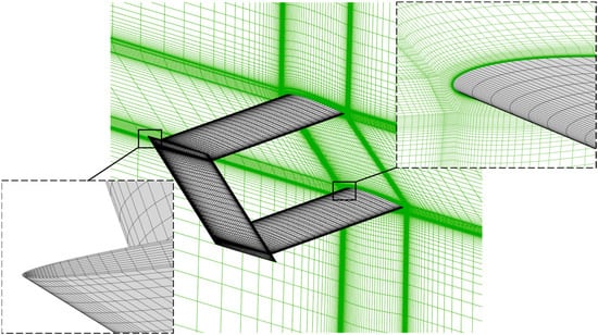
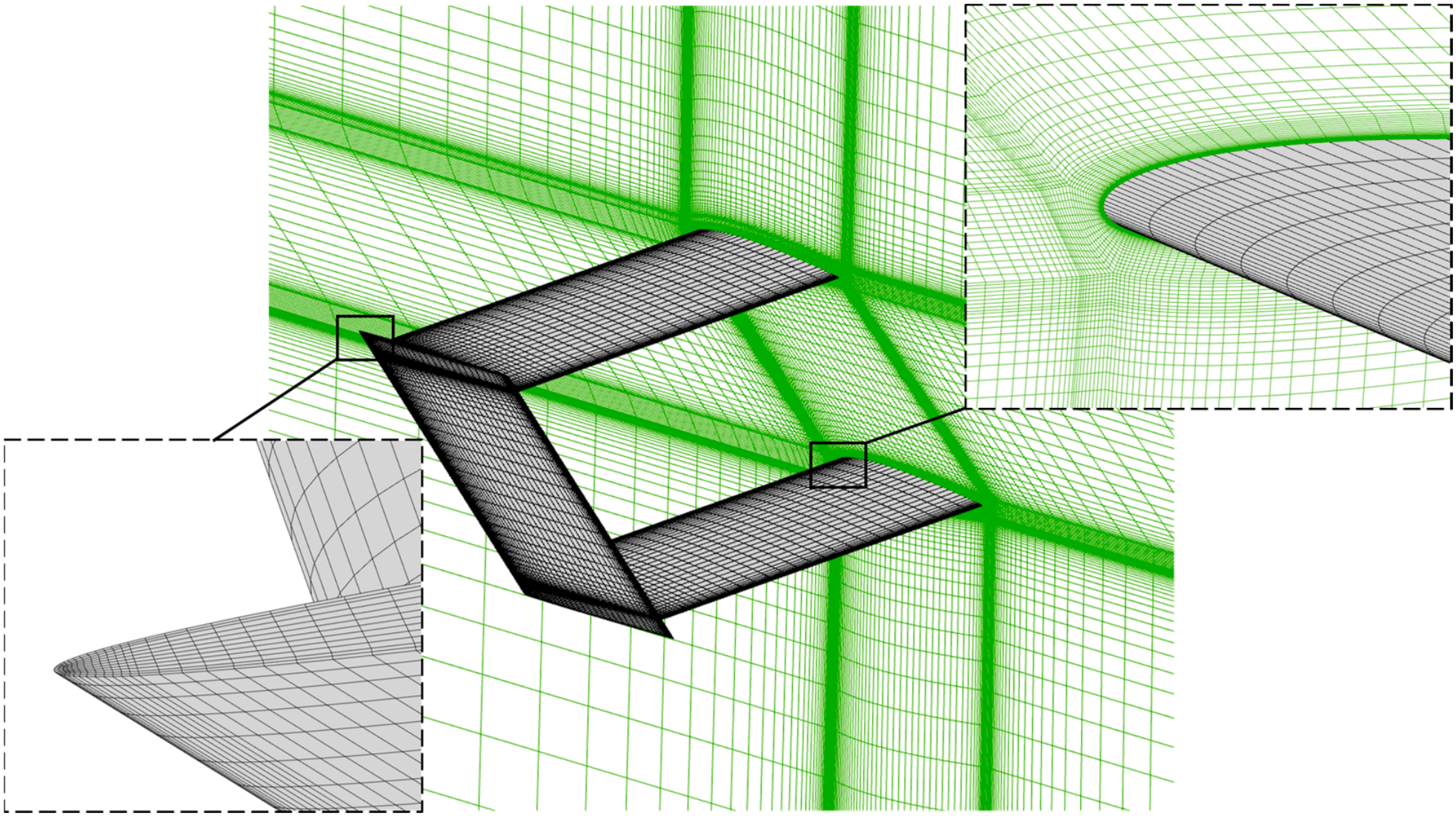
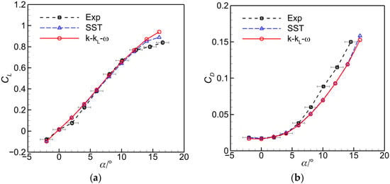
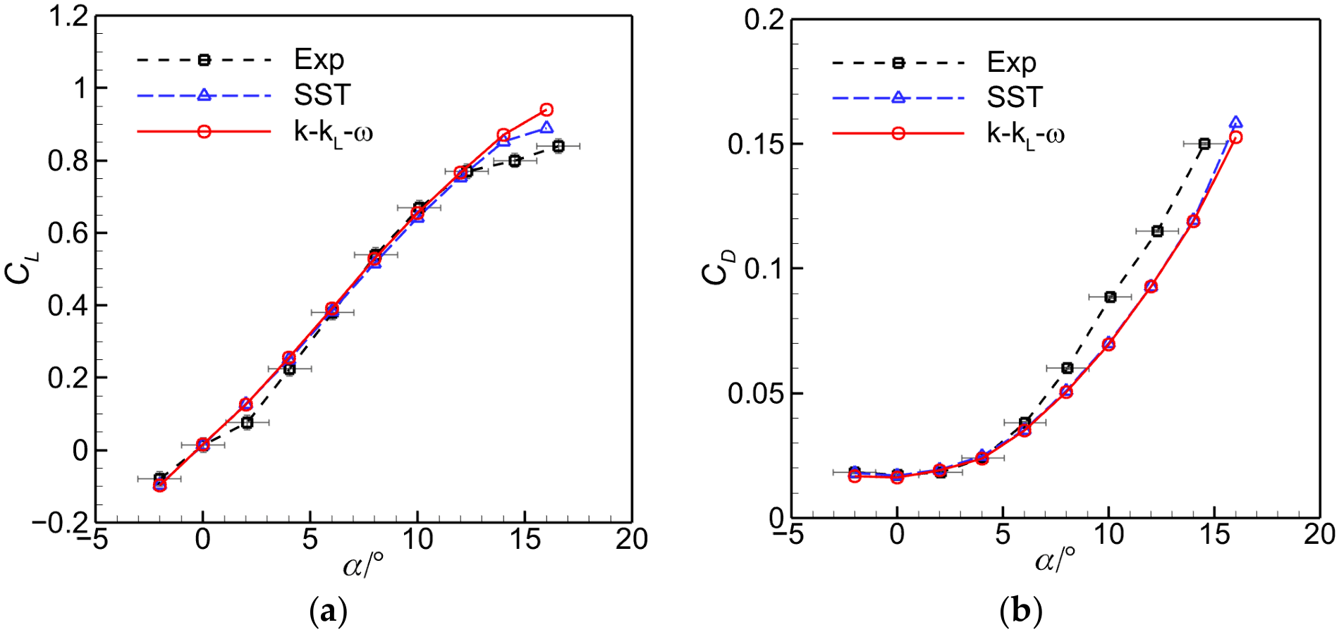
A biplane configuration with winglets was simulated to further validate the present method for three-dimensional flows. The model consists of two identical wings with a decalage angle of 0°. Both the vertical and horizontal spacing between the two wings are set to one chord length. The model and experimental results are reported in Ref. [22]. The Reynolds number is 5.1 × 10⁵. Both the SST and k-k_L-ω models were examined. The mesh contains approximately 3.1 million cells, as shown in Figure 3. The numerical results are presented in Figure 4. The calculations reproduce the overall lift and drag trends, with discrepancies at α = 2° and α > 8° and drag underprediction over part of the moderate-to-high-angle-of-attack range. The two turbulence models yield generally similar predictions, with only minor differences observed at α > 12°.

Figure 3. Computational mesh for the biplane configuration.

Figure 4. Comparison of the numerical and experimental results for the biplane configuration case: (a) lift coefficient; (b) drag coefficient.

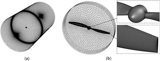
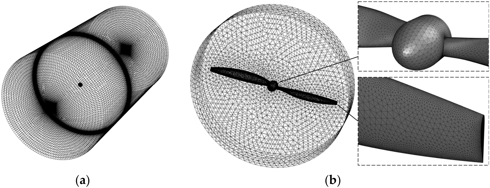
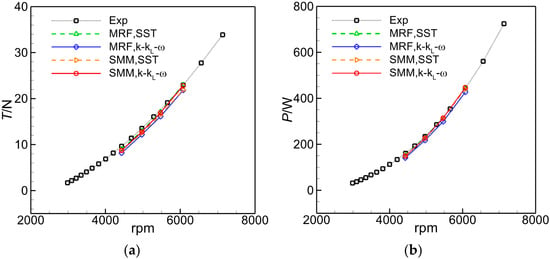
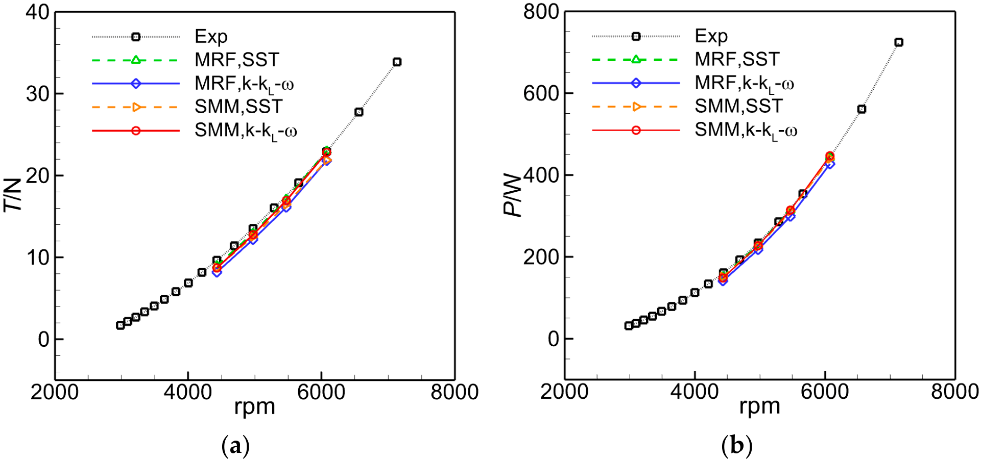
Finally, simulations of a two-bladed JXF 16 × 8 propeller were compared with the experimental data in Ref. [23]. The propeller radius is R = 0.203 m. The operating altitude is H = 400 m and the free-stream velocity is V_∞ = 11.1 m/s. Free-stream properties at different altitudes are derived from the corresponding standard atmosphere values in this paper. The mesh is shown in Figure 5. The rotating domain contains approximately 3.0 million cells, while the stationary outer domain contains approximately 1.9 million cells. The thrust and power characteristics predicted using two turbulence models with both the MRF method and SMM are compared with the experimental results, as shown in Figure 6. The calculated thrust and shaft power follow the experimental trends closely. For the isolated propeller under uniform inflow conditions, the flow and aerodynamic loading are nearly steady in the rotating reference frame. Therefore, the quasi-steady assumption adopted in the MRF approach is reasonable, resulting in similar time-averaged performance predictions from the MRF and SMM approaches. Although the Reynolds number based on the blade chord at 70% of the propeller radius is approximately 1.2 × 10⁵–1.8 × 10⁵, the two turbulence models yield similar predictions, suggesting that the integral propeller performance is relatively insensitive to transition modeling under the operating conditions considered here.

Figure 5. Computational mesh for the propeller case: (a) global view; (b) near-field view.

Figure 6. Comparison of the numerical and experimental results for the propeller case: (a) thrust; (b) shaft power.

The component-level benchmarks assess the numerical approach, which is subsequently applied to investigate the propeller–wing interactions in Section 3 and Section 4. These benchmarks do not directly validate the coupled low-Reynolds-number aircraft or the in-house propeller used in Section 4, and further experimental data for the coupled configurations would help assess the model-form uncertainty.

3. Aerodynamic Effects of Propeller–Wing Arrangement

Four representative propeller–wing configurations were comparatively examined using a common propeller and wing geometry. The comparison provides qualitative guidance for the aircraft layout in Section 4.

3.1. Model Setup

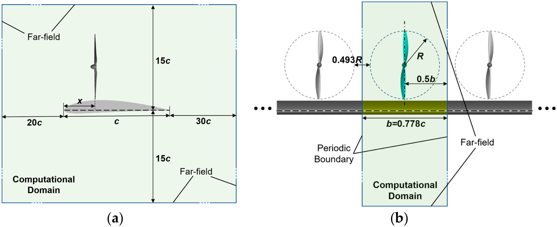
Periodic conditions at the two spanwise boundaries reduce computational cost by representing an infinite-span wing with a co-rotating propeller array. The model excludes counter-rotation, phase differences, and finite-span effects.

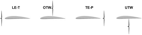
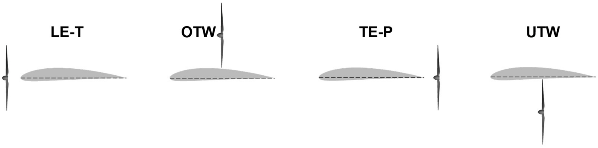
The propeller used in this section is the same as that described in Section 2.2, and the wing consists of a straight wing section with a NACA4412 airfoil. The propeller radius is R = 0.203 m, and the chord length of the wing section is c = 0.65 m. The spanwise length of the computational wing section is b = 0.506 m (0.778c), and the tip-to-tip clearance between adjacent propellers is 0.1 m (0.493R). The installation angle of the propeller relative to the wing is set to 0°, and the propeller support struts are neglected. The simulations are performed at an altitude of H = 400 m, a free-stream velocity of V_∞ = 11.1 m/s, an angle of attack α = 0° and a propeller rotational frequency of n = 101.25 s⁻¹ (corresponding to an advance ratio of J = 0.270). The schematic illustrations of the configurations are shown in Figure 7. The propeller–wing arrangements considered are summarized in Table 1. For comparison, two additional baseline cases are considered: an infinite-span wing without propellers and a distributed propeller array without the wing.

Figure 7. Schematic illustrations of different propeller–wing configurations.

Table 1. Summary of the propeller–wing arrangements considered in this study.

Configuration	Propeller Location	Normalized Streamwise Position of Propeller, xp/c	Normalized Tip-to-Wing Clearance, δ/R
Leading-edge tractor (LE-T)	Upstream of the wing; propeller center aligned with the wing chord line	−0.308, −0.154, −0.077	—
Over-the-wing (OTW)	Above the wing	0.1, 0.3, 0.5, 0.7, 0.9	0.0493; additional cases of 0.0148 and 0.148 at xp/c = 0.5
Trailing-edge pusher (TE-P)	Downstream of the wing; propeller center aligned with the wing chord line	1.077, 1.154	—
Under-the-wing (UTW)	Below the wing	0.5	0.0493

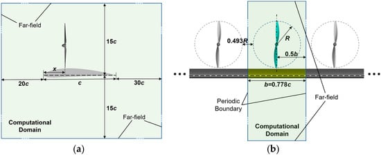
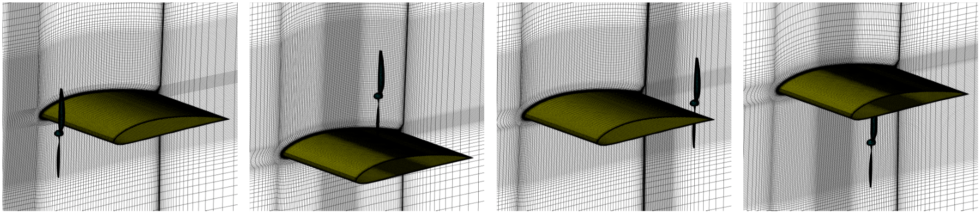
The free-stream chord Reynolds number is Re_c,∞ = ρ_∞V_∞ c/μ_∞ ≈ 4.8 × 10⁵. An estimated characteristic slipstream-core speed gives Re_c,slip = ρ_∞V_slip c/μ_∞ ≈ 9.9 × 10⁵. As the primary objective of Section 3 is to identify the main aerodynamic effects of different propeller–wing arrangements, the SST model is adopted as a computationally efficient approach for the comparison of the configurations. The computational domain and boundary conditions are shown in Figure 8. The propeller rotating region is discretized using unstructured meshes, and prism layers are generated to resolve the boundary layers. The first-layer height is controlled to achieve y⁺ ≈ 1 over most of the blade surface. The rotating region contains approximately 3.0 million cells. The stationary region, which includes the wing surface and the surrounding flow field excluding the propeller rotating regions, is discretized using structured grids. The first-layer height on the wing surface is also set to achieve y⁺ ≈ 1. Mesh refinement is applied around the wing’s leading and trailing edges and the propeller installation regions. Depending on the propeller location, the stationary region contains approximately 5.0–5.6 million cells. The mesh is shown in Figure 9. The simulations were performed using SMM. The computational method is the same as that described in Section 2.1.

Figure 8. Computational domain of the distributed propeller–wing configuration (the OTW configuration is taken as an example; the far-field boundaries are not drawn to scale): (a) side view; (b) front view.

Figure 9. Computational meshes of the distributed propeller–wing configurations (one representative mesh is shown for each configuration).

Separate grid and time-step checks were performed for OTW at x_p/c = 0.5. The grid comparison uses 8.3 and 11.2 million cells in the complete domain at 1° per time step; the time-step comparison reduces the increment to 0.5° on the 8.3-million-cell grid. The maximum cycle-averaged coefficient differences are 0.67% and 0.63%, respectively (Table 2).

Table 2. Grid and time-step sensitivity of the OTW configuration at x_p/c = 0.5.

Comparison	CL,w (%)	CD,w (%)	Cm,w (%)	CT (%)	CP (%)
Grid refinement	−0.30	−0.58	−0.63	−0.10	+0.67
Time-step refinement	−0.29	+0.63	−0.57	−0.07	−0.01

Percentage differences are 100 × (original result − refined result)/refined result. The refined result is the fine-grid result for the first row and the smaller-time-step result for the second.

3.2. Effects of Propeller–Wing Arrangement on Aerodynamic and Propulsive Characteristics

Figure 10 compares the aerodynamic and propulsive characteristics of the wing, the propeller subsystem, and the coupled propeller–wing system for the arrangements considered. All coefficients are time-averaged over one revolution. The abscissa x_p/c denotes the normalized chordwise propeller position, measured from the wing leading edge. The subscript w denotes the wing contribution; C_T and η are the propeller thrust coefficient and propeller efficiency, respectively; the superscript * denotes the coupled propeller–wing system; and the superscript ref identifies the corresponding uncoupled reference configuration, namely, the wing-only or DEP-only case. Some of the coefficients are defined as follows:

$$C_L^{*}={\displaystyle \frac{L_{\mathrm{w}}+F_{N,\mathrm{prop}}\cos \alpha +T_{\mathrm{prop}}\sin \alpha }{0.5\rho V_{\mathrm{\infty }}^{2}S}}$$

(1)

$$C_T={\displaystyle \frac{T_{\mathrm{prop}}}{\rho n^2{d}^4}}$$

(2)

$$C_X^{*}={\displaystyle \frac{F_X^{*}}{0.5\rho V_{\mathrm{\infty }}^{2}S}}={\displaystyle \frac{T_{\mathrm{prop}}\cos \alpha -F_{N,\mathrm{prop}}\sin \mathsf{\alpha }-D_{\mathrm{w}}}{0.5\rho V_{\mathrm{\infty }}^{2}S}}$$

(3)

$${\eta }^{*}={\displaystyle \frac{F_X^{*}{V}_{\mathrm{\infty }}}{P}}$$

(4)

$$C_m^{*}=C_{m,\mathrm{w}}+C_{m,\mathrm{prop}}$$

(5)

Here, the subscript prop denotes the propeller contribution. T_prop, F_N,prop, and P are the propeller thrust, propeller normal force, and propeller shaft power, respectively. n is the rotational frequency in revolutions per second, d is the propeller diameter, and S is the wing reference area. Propeller thrust and the net streamwise force of the coupled system are taken as positive in the forward direction, whereas wing drag is positive in the rearward direction. All pitching moment coefficients are based on the quarter-chord reference point. C_m,prop is the moment generated by the propeller about the reference point.

Figure 10. Effects of the propeller position on the aerodynamic and propulsive performance of different propeller–wing arrangements: (a) lift coefficients; (b) streamwise-force coefficients; (c) propulsive efficiencies; (d) pitching moment coefficients. ‘◁’, LE-T, leading-edge tractor configuration; ‘△’, OTW, over-the-wing configuration; ‘▷’, TE-P, trailing-edge pusher configuration; ‘▽’, UTW, under-the-wing configuration.

Figure 10. Effects of the propeller position on the aerodynamic and propulsive performance of different propeller–wing arrangements: (a) lift coefficients; (b) streamwise-force coefficients; (c) propulsive efficiencies; (d) pitching moment coefficients. ‘◁’, LE-T, leading-edge tractor configuration; ‘△’, OTW, over-the-wing configuration; ‘▷’, TE-P, trailing-edge pusher configuration; ‘▽’, UTW, under-the-wing configuration.

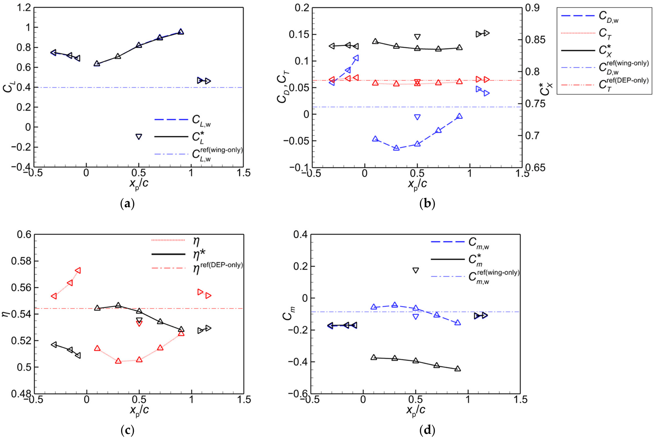
The subsystem metric η* evaluates installed propulsive performance from the coupled system’s net streamwise force and shaft power. Unlike propeller efficiency η, it captures changes in both propeller thrust and wing axial force. It compares arrangements at the prescribed operating conditions and is not an overall efficiency for a complete aircraft in trimmed steady flight, where net streamwise force is zero.

Among the examined cases, OTW produces the largest lift increase. Its coupled-system lift coefficient increases as the propeller moves aft, reaching the highest sampled value at x_p/c = 0.9. The net propulsive efficiency η* remains close to the DEP-only reference for x_p/c = 0.1–0.5, and reaches its highest sampled value at x_p/c = 0.3. The coupled OTW system also produces a substantial nose-down moment. All moments use a common geometric reference and describe aerodynamic loading rather than trim about the actual center of gravity. Wing-surface moments become more nose-down than the baseline in all cases except OTW at x_p/c = 0.1–0.5. There, the less-negative wing moment contrasts with the much more negative coupled-system moment, indicating that the additional nose-down moment arises mainly from the propeller, notably its forward thrust above the quarter-chord reference.

LE-T also provides a large lift increase. Moving the propeller closer to the wing increases η but reduces η*, because the increase in wing drag outweighs the improvement in propeller performance. This shows why installation effects require a coupled-system metric rather than propeller efficiency alone.

The TE-P configuration produces a more modest lift increase. At the same rotational speed, it gives the largest $C_X^{*}$ among the configurations considered. However, its shaft power is higher than that of the DEP-only reference, and its η* remains below the reference value. Among the arrangements considered, the pitching moment of the TE-P configuration remains closest to that of the wing-only case.

The LE-T and TE-P configurations increase both wing drag and propeller thrust relative to the corresponding reference cases. By contrast, the wing experiences a forward axial force in the OTW and UTW configurations, corresponding to a negative C_D,w under the present sign convention, while propeller thrust decreases slightly.

For UTW at x_p/c = 0.5, the coupled-system lift becomes negative and the propeller installation induces a pronounced nose-up pitching moment.

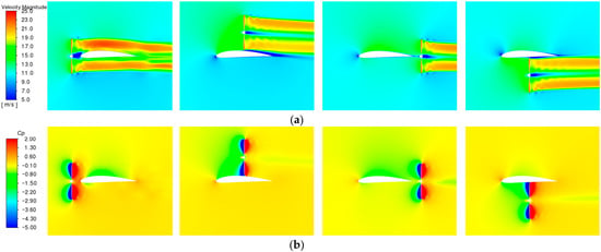
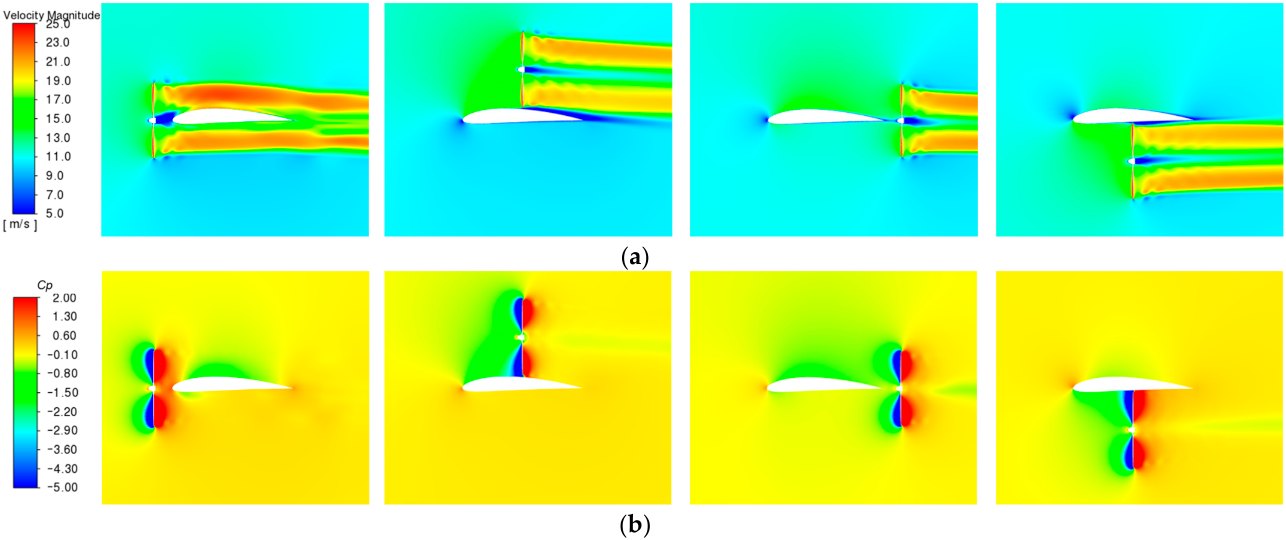
Figure 11 shows instantaneous velocity-magnitude and pressure-coefficient C_p contours through the propeller axis. The LE-T wing lies in the downstream slipstream, whereas the TE-P wing is affected mainly by weaker upstream induction. Flow acceleration increases the local dynamic pressure around the wing. OTW and UTW mainly redistribute pressure on the wing surface facing the propeller. For OTW, low pressure ahead of the disk enhances upper-surface suction over a chordwise extent that depends on propeller location.

Figure 11. Representative instantaneous contours in the longitudinal plane through the propeller center for different propeller–wing configurations: (a) velocity magnitude; (b) pressure coefficient. From left to right: LE-T (x_p/c = −0.154); OTW (x_p/c = 0.5); TE-P (x_p/c = 1.154); and UTW (x_p/c = 0.5).

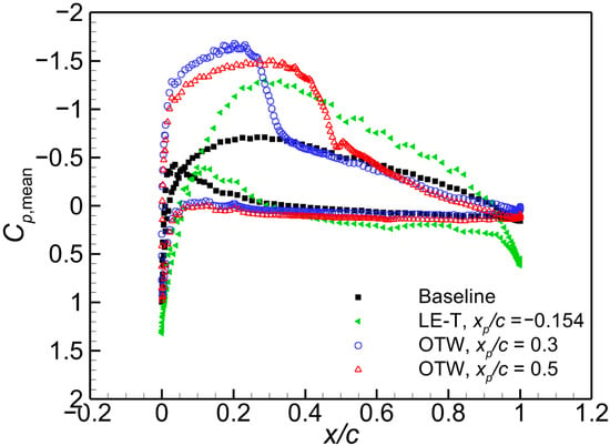
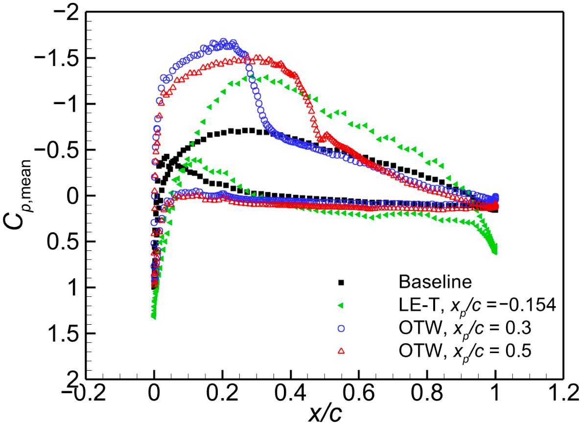
The cycle-averaged pressure distributions in Figure 12 resolve this response on the wing section through the propeller axis. Relative to the unpowered baseline, both OTW cases show enhanced upper-surface suction mainly upstream of the disk. Moving the propeller from x_p/c = 0.3 to 0.5 extends this region and shifts pressure recovery aft, consistent with the slightly less nose-down wing moment at 0.3 than at 0.5 in Figure 10d.

Figure 12. Cycle-averaged pressure-coefficient distributions on the wing section through the propeller axis for the unpowered baseline, LE-T (x_p/c = −0.154), and OTW (x_p/c = 0.3 and 0.5) arrangements at the conditions of Section 3.

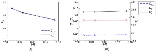
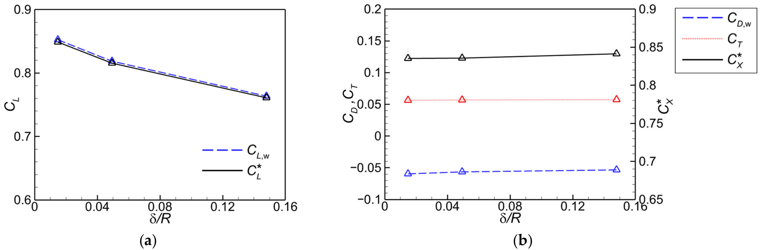
Figure 13 shows the effects of the normalized propeller-tip clearance (δ/R) on the OTW arrangement at x_p/c = 0.5. As δ/R increases from approximately 0.015 to 0.148, $C_L^{*}$ decreases by about 10.4%, whereas C_T and $C_X^{*}$ change by only about 1.6% and 0.7%, respectively. Within the range examined, the streamwise-force characteristics are relatively insensitive to clearance, while the lift augmentation weakens as the propeller is moved away from the wing.

Figure 13. Variations in the lift and streamwise-force coefficients with normalized propeller tip-to-wing clearance for the OTW (x_p/c = 0.5): (a) lift coefficients; (b) streamwise-force coefficients.

Under the present conditions, propeller–wing interaction changes wing loading more than propeller thrust and efficiency, allowing the arrangement to tailor installed performance.

4. Performance of a Hand-Launched UAV with a Propeller-Aided Biplane Configuration

The upstream-induction and downstream-slipstream mechanisms identified in Section 3 and earlier double-wing studies [16,18] motivate placing the propellers above the lower wing and ahead of the upper wing. The following sections compare PAB and CONV under clean, powered-cruise, and hand-launch conditions.

4.1. Aircraft Configuration, Numerical Assessment, and Baseline Aerodynamics

4.1.1. Aircraft Configuration and Design Conditions

The PAB aircraft and the CONV reference are defined under the common mission requirements in Table 3, with comparable overall wing dimensions. The common mass of 3 kg is consistent with the hand-launched UAV scale in Ref. [17], which also reports the group’s earlier MY-01 prototype. The prescribed mass and reference center-of-gravity positions below are not derived from a detailed component mass budget but are specified design values.

Table 3. Common mission requirements and design constraints for the two hand-launched UAV configurations.

Parameter	Design Value
Total mass	3.0 kg
Hand-launch altitude	500 m
Hand-launch speed	5.0 m/s
Hand-launch total shaft-power limit	≤600 W
Cruise altitude	2000 m
Cruise speed	15.0 m/s
Cruise total shaft-power limit	≤60 W
Propeller number	4
Propeller diameter	0.2 m

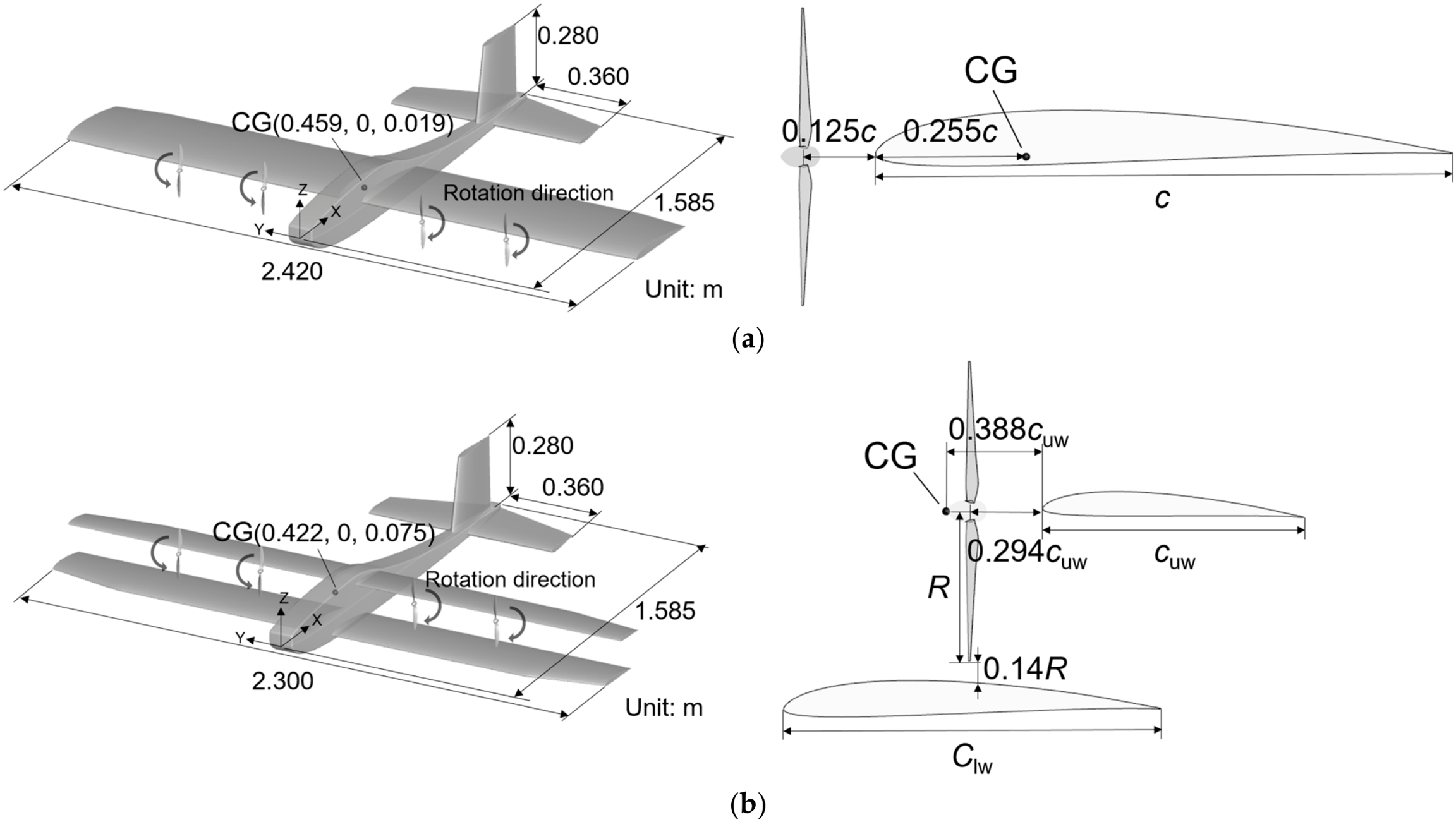
Both aircraft use the same fuselage, empennage, and in-house-designed propeller. CONV uses a leading-edge tractor arrangement; PAB places the propellers above the lower wing and upstream of the upper wing. The upper-wing incidence relative to the lower wing is 2°, and the propeller incidence is 0°. Table 4 and Figure 14 give the wing parameters and layouts. CONV and PAB have total wing areas of 0.952 and 0.958 m² and spans of 2.42 and 2.3 m, respectively. For a preliminary geometric comparison, the classical biplane model [24] gives a PAB equivalent monoplane aspect ratio (EMAR) of approximately 6.3, close to the CONV aspect ratio.

Table 4. Wing parameters of two configurations.

Parameter	Conventional Tractor Configuration (CONV)	Propeller-Aided Biplane Configuration (PAB)
		Lower Wing	Upper Wing
Airfoil	SD7037
Wing area	0.952 m2	0.570 m2	0.388 m2
Wing span	2.42 m	2.3 m	2.3 m
Chord length	0.40 m	0.25 m	0.17 m
Stagger (horizontal spacing)	—	0.175 m
Gap (vertical spacing)	—	0.136 m
Aspect-ratio metric	6.1	EMAR ≈ 6.3

Figure 14. The perspective and side views of the hand-launched UAV: (a) conventional tractor configuration (CONV); (b) propeller-aided biplane configuration (PAB).

The center-of-gravity (CG) positions in Figure 14 are layout-selected design reference points for all aircraft pitching moments. For both configurations, the resultant axial thrust line passes approximately through the CG, minimizing its direct pitching moment. The moment-coefficient reference length is the main-wing chord (0.4 m) for CONV and the sum of the two wing chords (0.42 m) for PAB.

The notation used in Section 4 distinguishes complete-aircraft resultants, denoted by the subscript total, and quantities summed over the four propellers, denoted by the subscript Σ. That is, $T_{\mathsf{\Sigma }}={\sum }_{i=1}^4{T}_i$ and $P_{\mathsf{\Sigma }}={\sum }_{i=1}^4{P}_i$, and η_Σ = T_ΣV_∞ cos α/P_Σ represents the aggregate installed propeller efficiency. The subscript af denotes the airframe contribution.

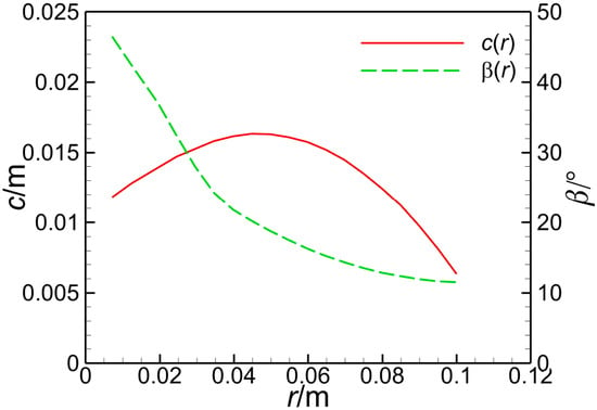
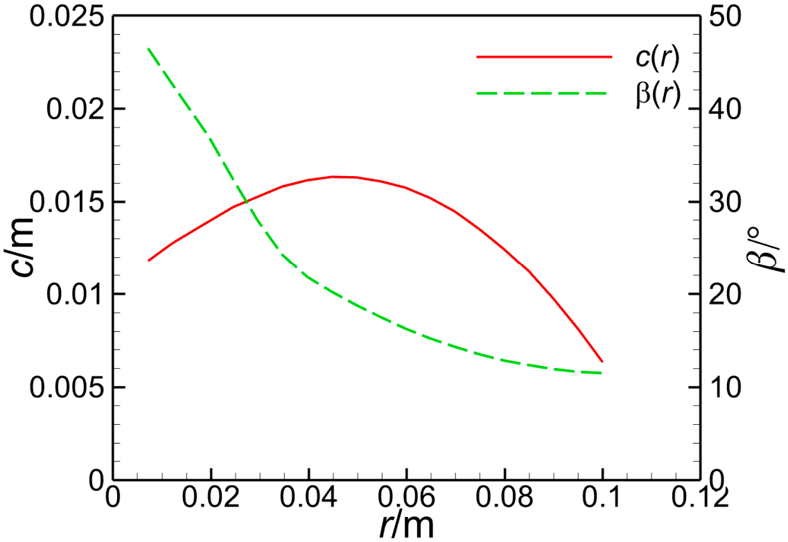
The four propellers use the same two-bladed, 0.20 m diameter geometry with Clark Y sections. Figure 15 gives the radial chord and blade-angle distributions, with blade angle measured relative to the plane of rotation. On each side, the inboard and outboard propellers rotate in the same direction and have identical initial phases.

Figure 15. Radial chord and blade-angle distributions of the in-house propeller.

The complete-aircraft resultants include the airframe and all four propellers. For propeller i, T_i is axial thrust; N_i is normal force, positive upward normal to the forward propeller axis; and M_CG,i is its pitching moment about the selected CG. In Equations (6)–(8), F_X,total is positive in the flight direction. Shaft power is P_i = 2πnQ_i, where Q_i is torque, and P_Σ = ΣP_i. The propeller power coefficient is C_P = P_i/(ρ_∞n³d⁵).

$$L_{\mathrm{total}}=L_{\mathrm{af}}+{\sum }_{i=1}^4(T_i\sin \alpha +N_i\cos \alpha ),$$

(6)

$$F_{X,\mathrm{total}}=-D_{\mathrm{af}}+{\sum }_{i=1}^4(T_i\cos \alpha -N_i\sin \alpha ),$$

(7)

$$M_{\mathrm{CG},\mathrm{total}}=M_{\mathrm{CG},\mathrm{af}}+{\sum }_{i=1}^4{M}_{\mathrm{CG},i}$$

(8)

Lift and forward-force effectiveness are defined as the cycle-mean L_total and F_X,total divided by the cycle-mean P_Σ. Equal rotational speed does not imply equal shaft power, and in the following lift-per-power differences describe operating-point effectiveness rather than lift gains at matched power.

4.1.2. Assessment of Turbulence Model and Baseline Aerodynamics

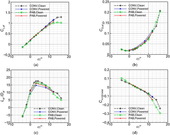
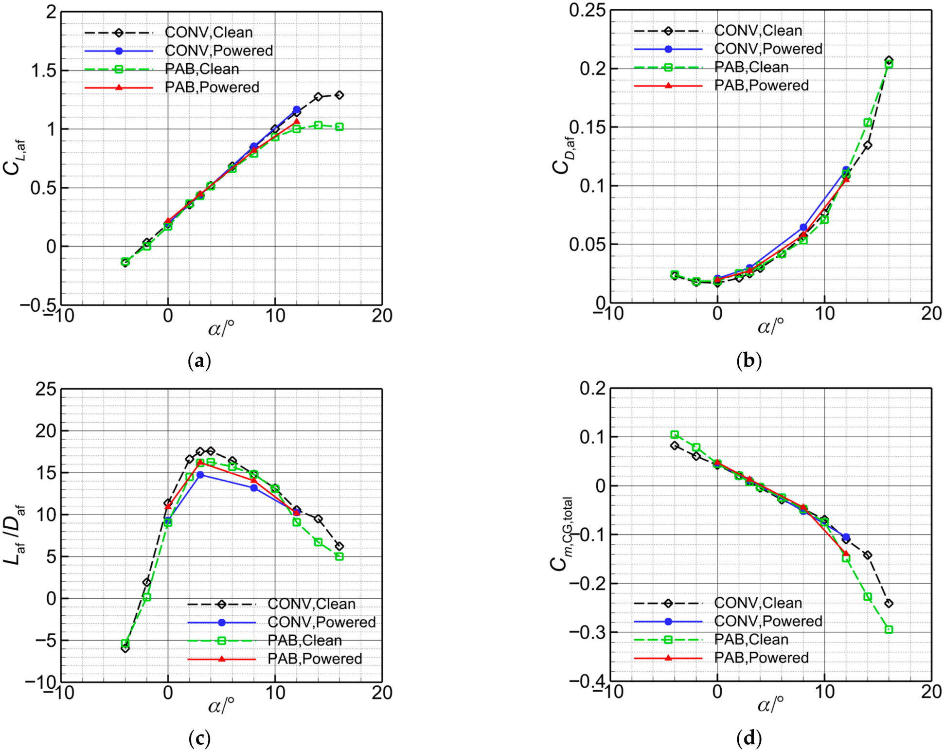
At cruise, the chord Reynolds numbers are approximately 3.5 × 10⁵ for CONV and 2.2 × 10⁵ and 1.5 × 10⁵ for the PAB lower and upper wings, respectively. The clean configurations are simulated using the fully turbulent SST and transition k-k_L-ω models to assess sensitivity to transition modeling and select the model for subsequent analyses.

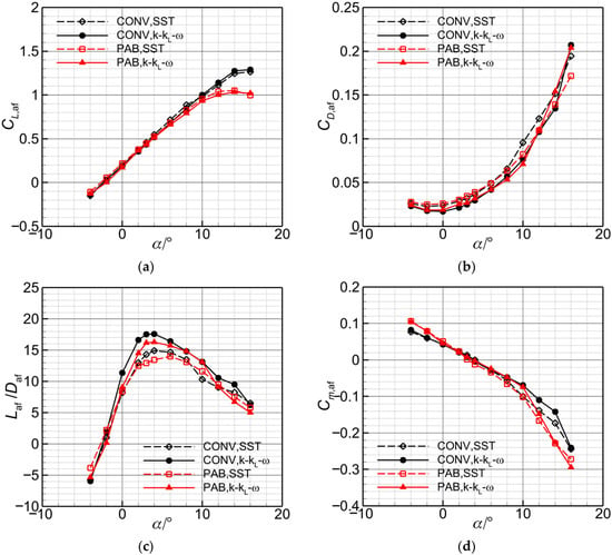
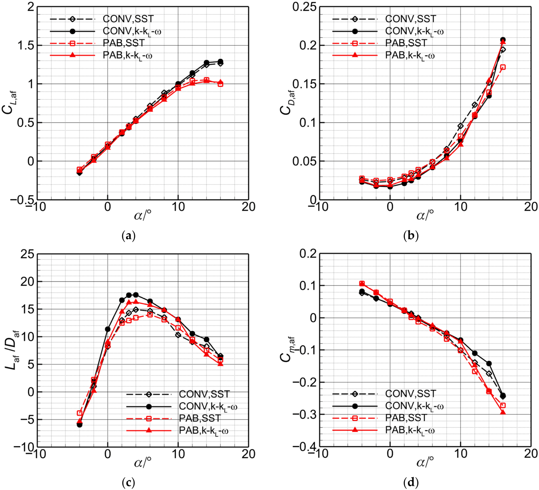
Figure 16 compares C_L,af, C_D,af, airframe lift-to-drag ratio L_af/D_af, and C_m,af over the investigated angle-of-attack range. In the near-linear lift range, the two models give similar lift and pitching moment trends for both configurations, whereas the SST model consistently predicts higher drag at low and moderate angles of attack. At α = 3°, the SST model predicts lift-to-drag ratios of approximately 14.2 for CONV and 12.9 for PAB, compared with 17.6 and 16.2, respectively, from the transition model. There is a nearly 20% difference between the predictions of the two models.

Figure 16. Aerodynamic characteristics of the clean configurations predicted using the SST and k-k_L-ω models (H = 2000 m, V_∞ = 15 m/s): (a) lift coefficient; (b) drag coefficient; (c) lift-to-drag ratio; (d) pitching moment coefficient.

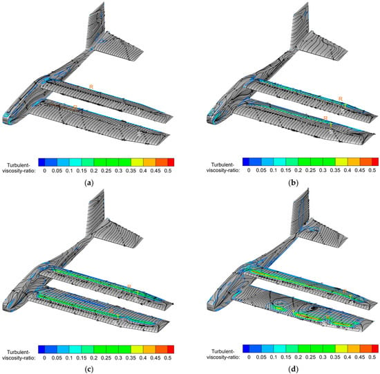
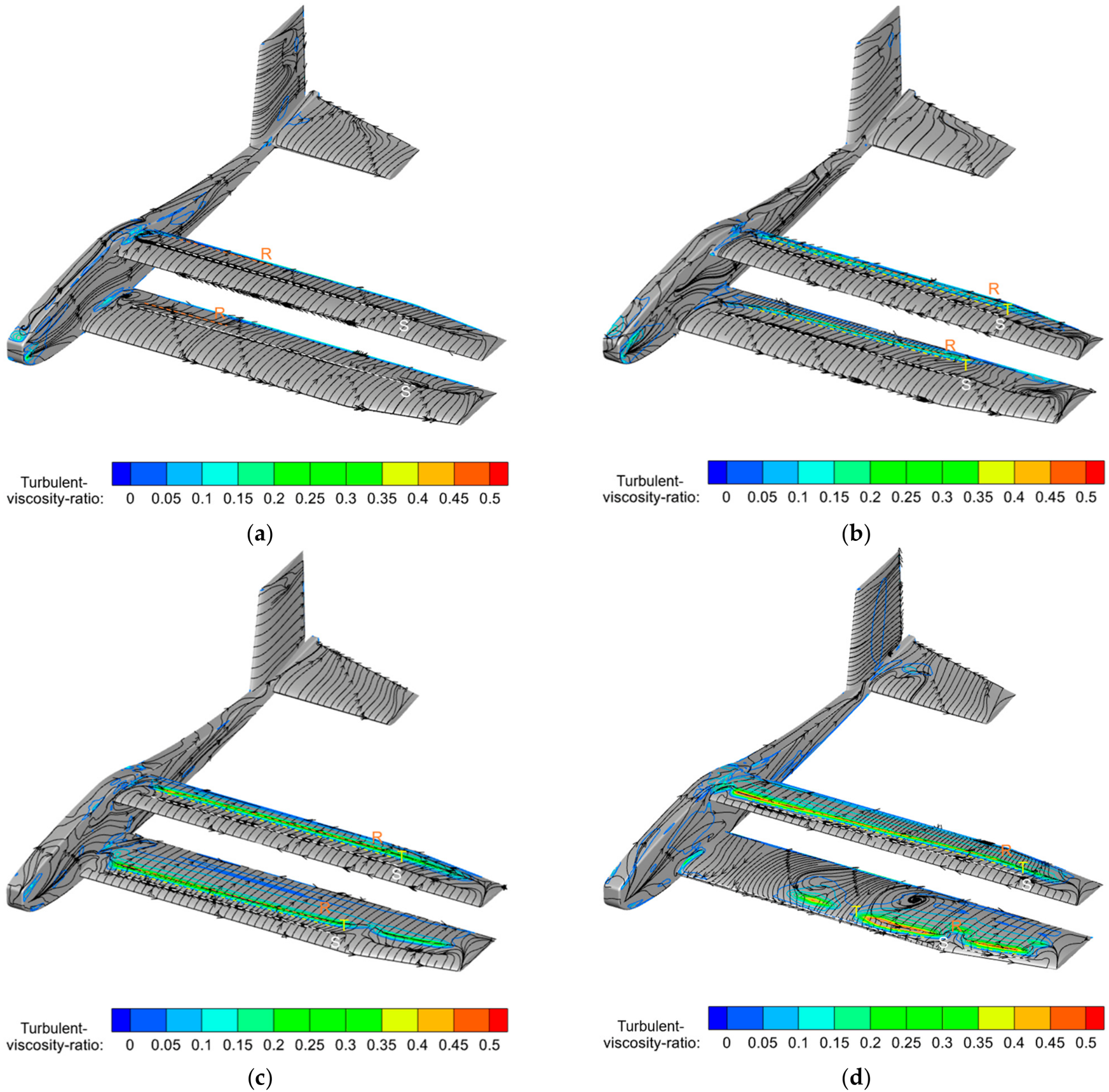
Figure 17 shows the turbulent-viscosity ratio (μ_t/μ) and surface streamlines predicted by the k-k_L-ω model for PAB. Surface-flow topology identifies separation and reattachment, while a rapid increase in μ_t/μ qualitatively indicates transition. Large laminar regions persist at low angles of attack, and both wings exhibit separation, transition, and reattachment at moderate angles. As the angle increases, separation moves forward and spanwise nonuniformity strengthens. At α = 12°, much of the lower-wing flow is separated except near the tip. A fully turbulent model does not explicitly represent this transition, which helps explain the drag difference. Together with the validation of the k-k_L-ω model in Section 2.2, these results support its use in the subsequent analyses.

Figure 17. Turbulent-viscosity ratio and surface streamlines of the clean PAB configuration (H = 2000 m, V_∞ = 15 m/s): (a) α = 0°; (b) α = 3°; (c) α = 8°; (d) α = 12°. ‘S’ and ‘R’ indicate separation and reattachment from the surface-flow topology, respectively; ‘T’ marks a qualitative indication of transition.

At α = 12°, extensive separation over the forward lower wing and more organized separation–reattachment over the aft upper wing (Figure 17d) may explain the increasingly negative PAB moment in Figure 16d. Reduced lower-wing lift ahead of the selected CG would diminish its nose-up contribution relative to the upper wing’s nose-down contribution.

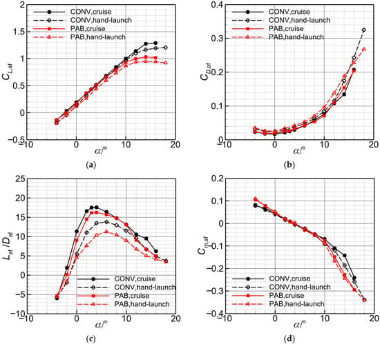
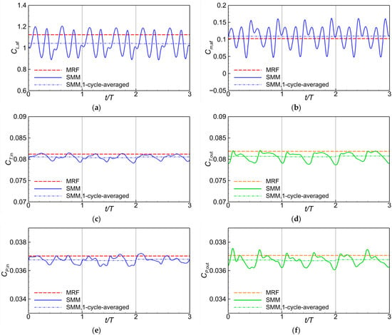
Figure 18 compares the clean-airframe baselines at cruise and hand launch. The lower launch Reynolds numbers lead to lower lift coefficients, higher drag coefficients over much of the sampled range, and a marked reduction in lift-to-drag ratio. PAB’s shorter chords, lower Reynolds numbers, and inter-wing interference may contribute to its larger efficiency penalty. PAB thus has no clean-airframe efficiency advantage at these conditions. Section 4.2 and Section 4.3 assess its powered performance.

Figure 18. Baseline aerodynamic characteristics of the clean configurations at the cruise (H = 2000 m, V_∞ = 15 m/s) and hand-launch (H = 500 m, V_∞ = 5 m/s) conditions: (a) lift coefficient; (b) drag coefficient; (c) lift-to-drag ratio; (d) pitching moment coefficient.

4.1.3. Assessment of Propeller Modeling

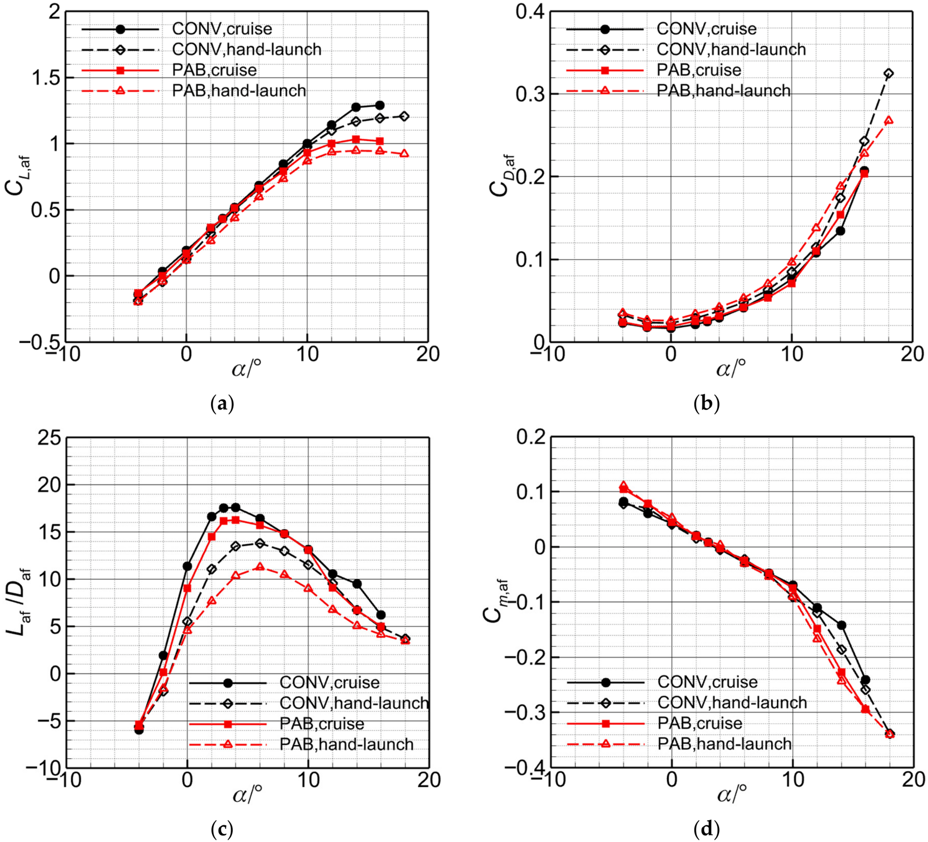
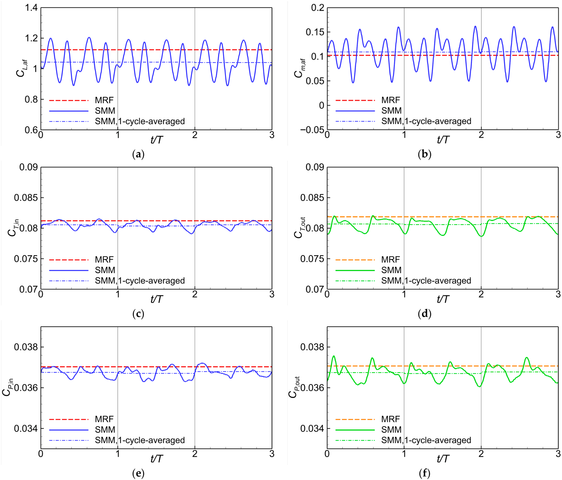
The PAB case at H = 500 m, V_∞ = 5 m/s, α = 4° and n = 216.67 s⁻¹ is discussed using steady MRF and unsteady SMM. Figure 19 shows three consecutive stabilized propeller revolutions with individual cycle means. SMM resolves phase-dependent airframe loads, whereas MRF gives steady loads. The mean airframe lift and pitching moment differ noticeably, but the mean inboard and outboard propeller thrusts are similar. The subscripts in and out denote the inboard and outboard propellers.

Figure 19. Comparison of MRF and SMM predictions over three consecutive propeller revolutions for the PAB configuration (H = 500 m, V_∞ = 5 m/s, α = 4° and n = 216.67 s⁻¹): (a) airframe lift coefficient; (b) airframe pitching moment coefficient; (c) inboard-propeller thrust coefficient; (d) outboard-propeller thrust coefficient; (e) inboard-propeller power coefficient; (f) outboard-propeller power coefficient. Each dash-dot SMM segment indicates the mean over the corresponding individual revolution.

For this representative case, the maximum absolute difference between successive cycle means is 0.55% among the six plotted coefficients. Comparing the final-revolution mean with averages over the final two and three revolutions gives a maximum difference of 0.32% (Table 5 and Table 6).

Table 5. Successive-cycle mean differences for the representative PAB case in Figure 19.

t/T	CL,af (%)	Cm,af (%)	CT,in (%)	CP,in (%)	CT,out (%)	CP,out (%)
0–1	—	—	—	—	—	—
1–2	0.02	−0.16	−0.27	−0.13	−0.12	−0.15
2–3	−0.20	0.55	0.26	0.24	0.23	0.23

Percentage differences are relative to the corresponding mean of the immediately preceding revolution.

Table 6. Sensitivity to one-, two-, and three-revolution averaging windows for the representative PAB case in Figure 19.

t/T	CL,af (%)	Cm,af (%)	CT,in (%)	CP,in (%)	CT,out (%)	CP,out (%)
2–3	—	—	—	—	—	—
1–3	0.10	−0.28	−0.13	−0.12	−0.11	−0.11
0–3	0.12	−0.32	−0.08	−0.11	−0.11	−0.10

Percentage differences are relative to the mean of the last revolution.

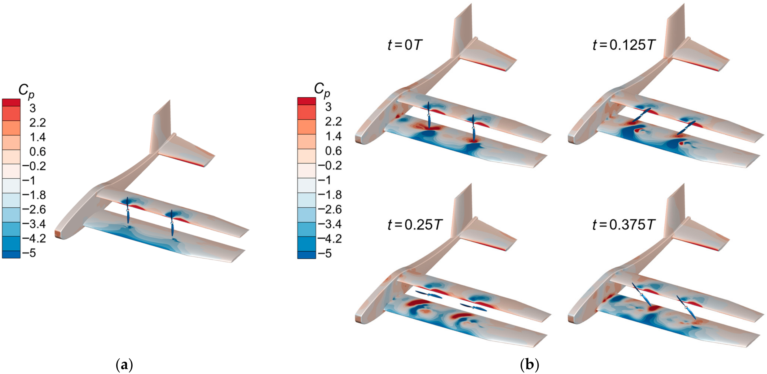
Figure 20 shows smooth, stationary pressure distributions for MRF and alternating high- and low-pressure patterns for SMM. The SMM patterns sweep across both wings with blade azimuth, redistributing the loading and accounting for the oscillations in C_L,af and C_m,af.

Figure 20. Surface pressure-coefficient distributions for the PAB configuration (H = 500 m, V_∞ = 5 m/s, α = 4° and n = 216.67 s⁻¹): (a) MRF prediction; (b) SMM predictions at t/T = 0, 0.125, 0.25, and 0.375.

The phase-dependent interaction limits the quasi-steady approximation: MRF and SMM give similar mean propeller thrust but different mean airframe loads. SMM is adopted for all subsequent calculations, and cycle-averaged quantities are used for performance comparisons.

4.1.4. Grid and Time-Step Sensitivity

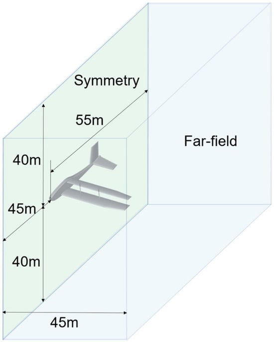
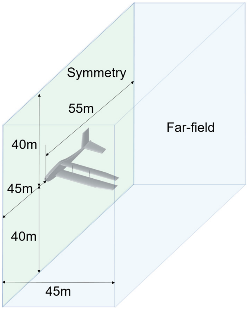
Mirror-symmetric propeller rotation and blade phases allow a half-aircraft model. This symmetry condition excludes sideslip, asymmetric propulsion or control inputs, and antisymmetric flow modes. Figure 21 shows the half-aircraft domain, with pressure-far-field outer boundaries, a longitudinal symmetry plane, and no-slip, adiabatic airframe and blade surfaces. The rotating zones exchange information with the stationary region through sliding interfaces.

Figure 21. Half-aircraft computational domain and boundary conditions (distances are in meters; the far-field boundaries are not drawn to scale).

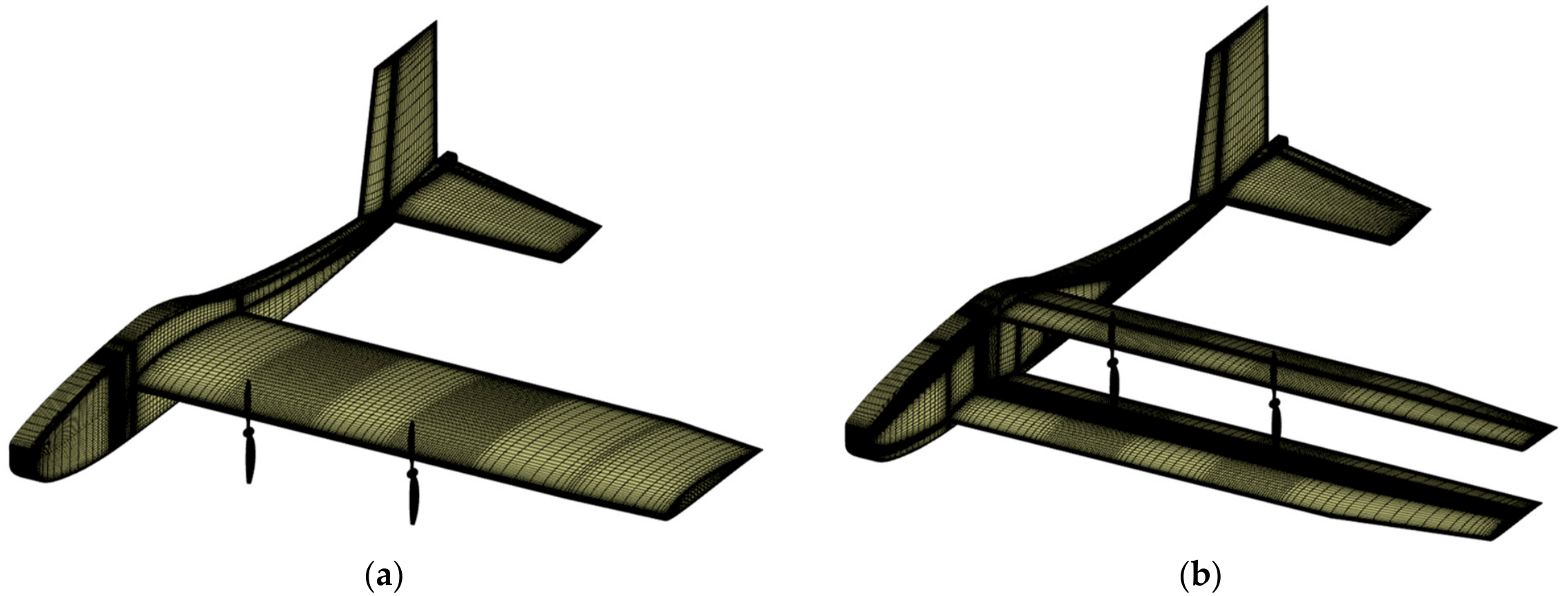
Grid sensitivity is assessed for both configurations at H = 500 m, V_∞ = 5 m/s, α = 4° and n = 216.67 s⁻¹ using k-k_L-ω and SMM. The hand-launch condition is selected to assess grid sensitivity for low-Reynolds-number flow with high propeller loading and strong propeller-induced velocity gradients. Three successively refined grids share the same first cell height, targeting y⁺ ≈ 0.5. Table 7 reports differences relative to the fine grids. Every monitored coefficient computed on the medium grid differs from its fine-grid value by no more than 2.2% for CONV and 1% for PAB. The medium grids of 14.8 and 16.5 million cells, respectively, are adopted to balance accuracy and cost. The adopted meshes are shown in Figure 22.

Table 7. Grid-convergence results for the half-aircraft models at α = 4° and V_∞ = 5 m/s.

Config.	Cells (million)	CL,af (%)	CD,af (%)	Cm,af (%)	CT,in (%)	CP,in (%)	CT,out (%)	CP,out (%)
CONV	9.1	−0.46	−2.54	−6.28	−2.71	−4.10	−2.62	−3.67
CONV	14.8	−0.24	−1.38	−2.15	−0.94	−0.92	−0.85	−0.88
CONV	21.3	—	—	—	—	—	—	—
PAB	9.8	0.62	−2.77	−6.27	−2.93	−3.95	−2.06	−2.64
PAB	16.5	−0.29	−0.98	−0.79	−0.65	−0.76	−0.98	−0.85
PAB	24.0	—	—	—	—	—	—	—

Percentage differences are relative to the corresponding fine-grid result.

Figure 22. Surface mesh of the adopted grids: (a) CONV configuration; (b) PAB configuration.

Separate grid and time-step checks are also performed at the 12° hand-launch condition. The grid check retains the 1° time step and uses the fine grids, and the time-step check retains the medium grids and reduces the rotation increment to 0.5°. Table 8 and Table 9 report the coefficient differences. The maximum absolute changes in C_L,total are 0.45% and 0.63% for grid and time-step refinement, respectively; those in individual propeller power coefficients are 0.79% and 0.65%, and those in C_m,af are 2.75% and 3.00%. These checks quantify discretization sensitivity, not a formal uncertainty interval.

Table 8. Grid sensitivity at the 12° hand-launch condition.

Config.	Cells (million)	CL,af (%)	CD,af (%)	Cm,af (%)	CL,total (%)	CT,in (%)	CP,in (%)	CT,out (%)	CP,out (%)
CONV	14.8	0.39	0.09	1.76	0.31	−0.16	−0.79	0.30	−0.68
CONV	21.3	—	—	—	—	—	—	—	—
PAB	16.5	−0.27	0.59	−2.75	−0.45	−0.49	−0.66	−0.39	−0.46
PAB	24.0	—	—	—	—	—	—	—	—

Percentage differences are 100 × (baseline − fine-grid result)/fine-grid result.

Table 9. Time-step sensitivity at the 12° hand-launch condition.

Config.	Step (deg.)	CL,af (%)	CD,af (%)	Cm,af (%)	CL,total (%)	CT,in (%)	CP,in (%)	CT,out (%)	CP,out (%)
CONV	1	0.54	0.05	1.05	0.63	0.69	−0.51	0.76	−0.23
CONV	0.5	—	—	—	—	—	—	—	—
PAB	1	0.04	−0.79	−3.00	0.25	0.46	−0.65	0.68	0.19
PAB	0.5	—	—	—	—	—	—	—	—

Percentage differences are 100 × (baseline − fine-step result)/fine-step result.

4.2. Cruise Performance

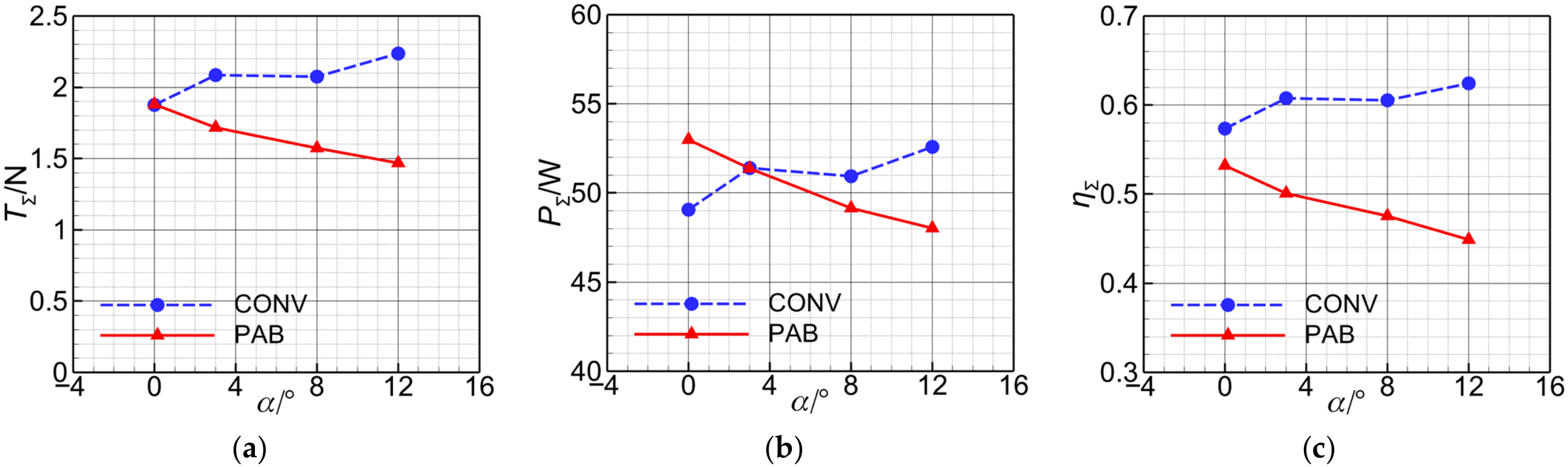
Figure 23 and Figure 24 compare CONV and PAB at H = 2000 m and V_∞ = 15 m/s, showing the airframe response and complete-aircraft pitching moment, and the cycle-averaged summed propeller quantities, respectively. The propeller rotational frequencies are 138.33 s⁻¹ for CONV and 150 s⁻¹ for PAB, and P_Σ remains below the 60 W limit throughout the sampled range. These speeds provide nearly the same T_Σ at α = 0°. The installed propeller loading varies with both angle of attack and arrangement. The results represent untrimmed fixed-rpm comparisons rather than a thrust-matched sweep or established cruise-power requirements.

Figure 23. Cruise aerodynamic characteristics of the CONV and PAB configurations at the cruise condition (H = 2000 m and V_∞ = 15 m/s): (a) airframe lift coefficient; (b) airframe drag coefficient; (c) airframe lift-to-drag ratio; (d) complete-aircraft pitching moment coefficient. The powered results are cycle-averaged and correspond to fixed propeller rotational frequencies of 138.33 s⁻¹ for CONV and 150 s⁻¹ for PAB.

Figure 24. Propeller performance of CONV and PAB at the cruise condition: (a) summed thrust of the four propellers; (b) summed shaft power of the four propellers; (c) aggregate installed propeller efficiency. The flight condition and propeller rotational frequencies are the same as those in Figure 23.

In CONV, the accelerated downstream slipstream changes C_L,af only slightly while increasing C_D,af at every sampled angle of attack (Figure 23). In PAB, upstream propeller induction primarily influences the lower wing, while the upper wing lies in the accelerated downstream slipstream. The powered-airframe drag of PAB remains close to the clean value at low-to-moderate angles of attack and becomes slightly lower at α = 12°. Its main effect is a smaller powered-airframe drag penalty, rather than a general drag reduction. PAB has the higher powered-airframe L/D over most of the low-to-moderate range; at α = 3°, the values are approximately 16.2 and 14.7 for PAB and CONV, respectively. The complete-aircraft pitching moment coefficients decrease with angle of attack for both configurations (Figure 23d). PAB is slightly less nose-down at the intermediate sampled angle, but this ordering reverses at the largest angle.

At α = 0°, Figure 24 gives T_Σ ≈ 1.88 N for both aircraft, P_Σ ≈ 49.1 W for CONV and 53.0 W for PAB, and corresponding η_Σ values of approximately 0.574 and 0.532. The lower PAB efficiency corresponds to similar thrust at greater shaft power. As angle of attack increases, T_Σ and η_Σ generally increase for CONV and decrease for PAB.

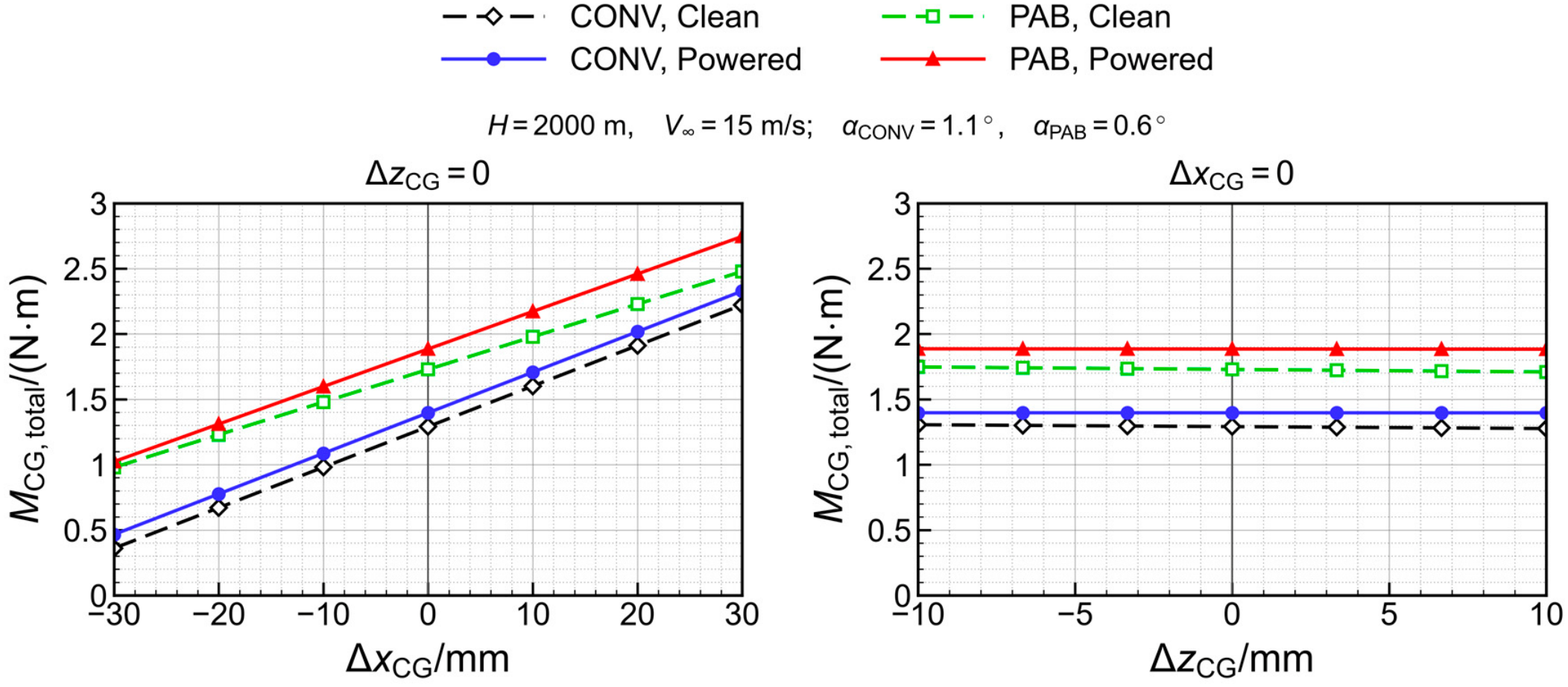
For the 3.0 kg design mass, the representative angles of approximately 1.1° for CONV and 0.6° for PAB are near-weight-supporting conditions. Approximate interpolation of the plotted results gives shaft powers of 49.9 and 52.7 W, streamwise-force residuals of −0.63 and −0.44 N, and nose-up moments of +1.40 and +1.89 N m, respectively. For these low-thrust, small-angle-of-attack conditions, the interpolated streamwise-force residuals omit the propeller normal-force contribution to the streamwise resultant.

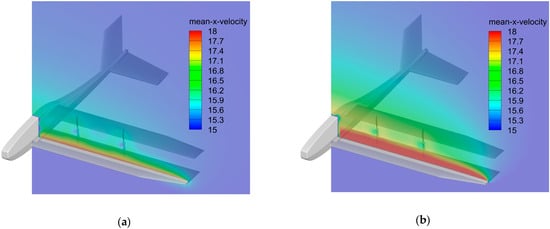
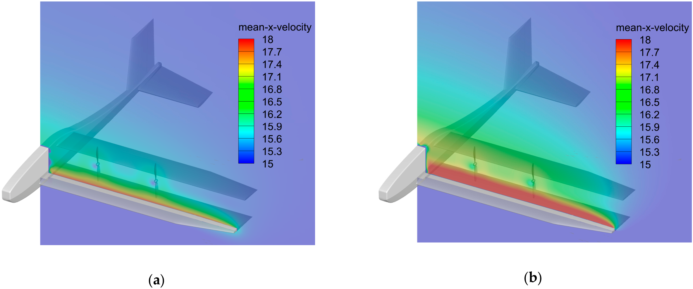
Figure 25 shows the cycle-averaged axial velocity 0.15d upstream of the PAB propeller disks at α = 0° and 8°. The elevated-velocity region above the lower wing extends farther across the disk locations at 8°. At fixed rotational speed and tangential velocity, an increase in local axial inflow increases the local inflow angle and reduces blade-section incidence, consistent with the falling PAB thrust and shaft power in Figure 24.

Figure 25. Cycle-averaged axial velocity upstream of the PAB propeller disks at H = 2000 m and V_∞ = 15 m/s: (a) α = 0°; (b) α = 8°. The plane is 0.15d upstream of the disks.

4.3. Hand-Launch Performance

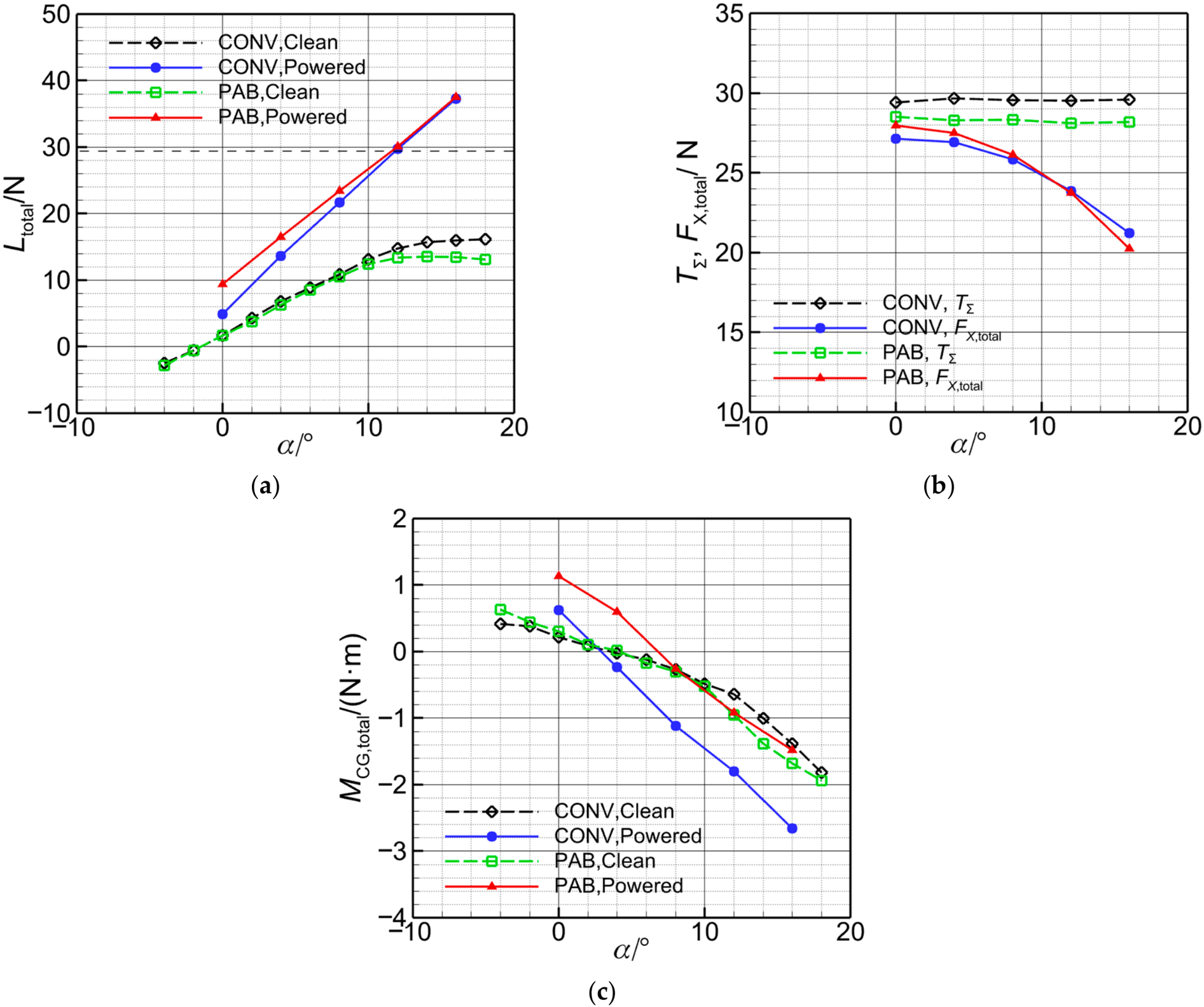
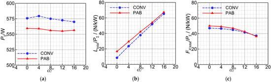
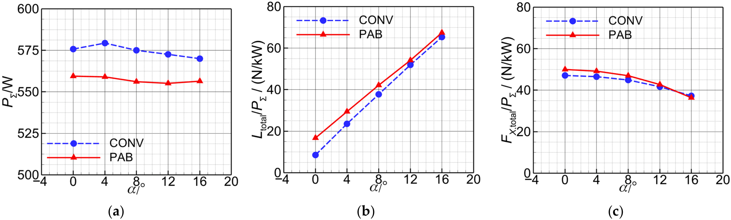
Both aircraft are evaluated at H = 500 m, V_∞ = 5 m/s, and a propeller rotational frequency of 216.67 s⁻¹. The resulting P_Σ values of approximately 555–580 W satisfy the 600 W design limit. Powered quantities are averaged over the final propeller revolution. Because free-stream-based coefficients become large at this speed, Figure 26 and Figure 27 present the dimensional loads L_total, F_X,total, and M_CG,total, shaft power, and force effectiveness.

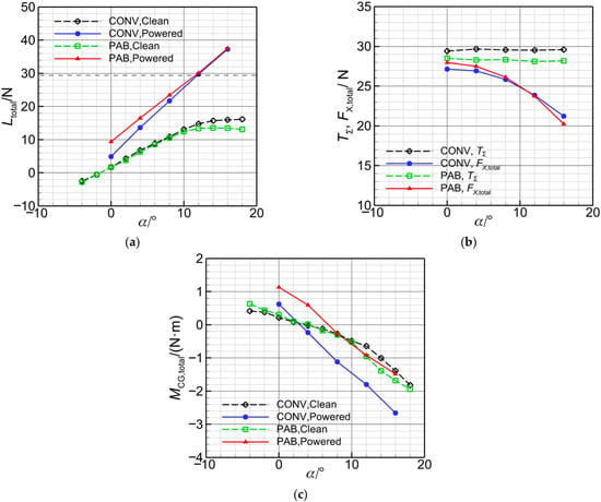
Figure 26. Force and pitching moment characteristics of the CONV and PAB configurations at the hand-launch condition (H = 500 m and V_∞ = 5 m/s): (a) total lift; (b) summed propeller thrust and complete-aircraft streamwise force; (c) pitching moment. Powered quantities are cycle-averaged and correspond to a fixed propeller rotational frequency of 216.67 s⁻¹.

Figure 27. Shaft power and force effectiveness of the powered CONV and PAB configurations at the hand-launch condition: (a) summed shaft power of the four propellers; (b) total lift per unit summed shaft power; (c) complete-aircraft streamwise force per unit summed shaft power.

In Figure 26a, the clean PAB lift curve levels off at large angles of attack, whereas powered L_total continues to increase through the final sampled point at 16°. PAB produces greater total lift than CONV throughout the powered sweep. At this low free-stream dynamic pressure, the loads depend strongly on installed propeller–wing interaction. At α = 12°, PAB and CONV total lifts are approximately 30.1 and 29.8 N, respectively, compared with the 29.4 N aircraft weight; corresponding shaft powers are 555.2 and 572.6 W. PAB also maintains greater lift effectiveness throughout the sampled range (Figure 27b). At 12°, ${{\mathrm{L}}_{\mathrm{total}}/\mathrm{P}}_{\mathsf{\Sigma }}$ is approximately 54.2 N/kW for PAB and 52.0 N/kW for CONV, a relative difference of 4.2%. The lift-effectiveness gain is also retained under the grid and time-step refinements in Table 8 and Table 9. The relative gain over CONV is approximately 4.2% for the baseline, 5.2% on the fine grids, and 4.7% at the smaller time step. The positive gain is retained, with changes of +1.0 and +0.5 percentage points under grid and time-step refinement, respectively.

Both configurations retain a large positive F_X,total throughout the sampled hand-launch range, with forward resultants of approximately 24 N near α = 12° (Figure 26b). PAB provides a slightly higher ${{\mathrm{F}}_{\mathrm{X},\mathrm{total}}/\mathrm{P}}_{\mathsf{\Sigma }}$, within 8–12°, producing comparable forward force at lower power (Figure 27c). Propeller efficiencies are similar at approximately 0.25, with PAB slightly lower. Its lift-effectiveness gain combines higher lift and lower shaft power. The positive forward resultant and smaller vertical-force deficit at the lower angle of attack are consistent with previous quasi-steady analyses of comparable hand-launched powered-lift UAVs, in which forward acceleration moves the aircraft toward a higher-lift speed [17].

Figure 26c shows smaller nose-down moments for PAB about the respective design CGs. At α = 8°, the PAB and CONV moments are approximately −0.26 and −1.12 N m; at 12°, they are −0.92 and −1.79 N m. Relative to their clean states, CONV develops a pronounced additional nose-down moment under power, whereas the PAB increment is much smaller. With the axial thrust lines close to the design CGs, this difference is consistent with changed combined airframe loading.

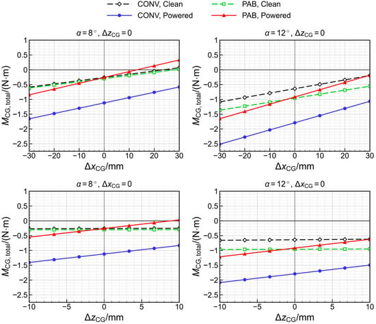
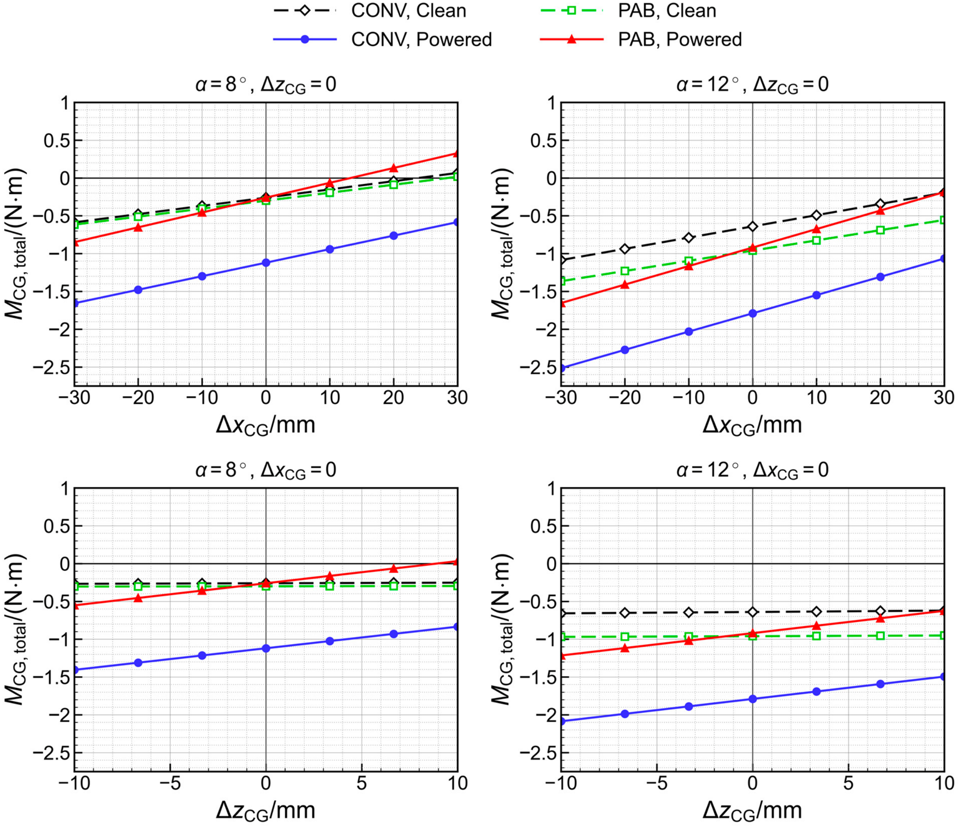
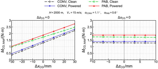
The dependence of the moment comparison on the reference CG is assessed for clean and powered hand-launch states at 8° and 12° and for the representative cruise states. Longitudinal shifts of ±30 mm and vertical shifts of ±10 mm are applied separately while holding the aerodynamic state fixed. With body x positive aft, z positive upward, and pitching moment positive nose-up, the reference translation is given by Equations (9)–(11).

M_new = M₀ + Δx_CGF_z,b − Δz_CGF_x,b

(9)

F_z,b = L_totalcosα − F_X,totalsinα

(10)

F_x,b = −F_X,totalcosα − L_totalsinα

(11)

Figure 28 and Figure 29 give reference-point sensitivity. At the nominal CGs, the PAB–CONV moment differences are approximately +0.86 and +0.87 N m at 8° and 12°, respectively. These reference-point translations hold the aerodynamic states fixed, and they do not define an achievable CG envelope or demonstrate trim or control authority.

Figure 28. Hand-launch pitching moment sensitivity to CG displacement at 8° (left) and 12° (right). Upper and lower rows show longitudinal and vertical shifts, respectively, with the other coordinate fixed. Clean and powered states use the same shifted reference point.

Figure 29. Sensitivity of cruise pitching moments to CG displacement. The left and right plots show longitudinal and vertical displacement, respectively, at the representative cruise angles (CONV: 1.1°; PAB: 0.6°). Clean and powered loads are interpolated at the same angle within each configuration. Clean and powered states use the same shifted reference point.

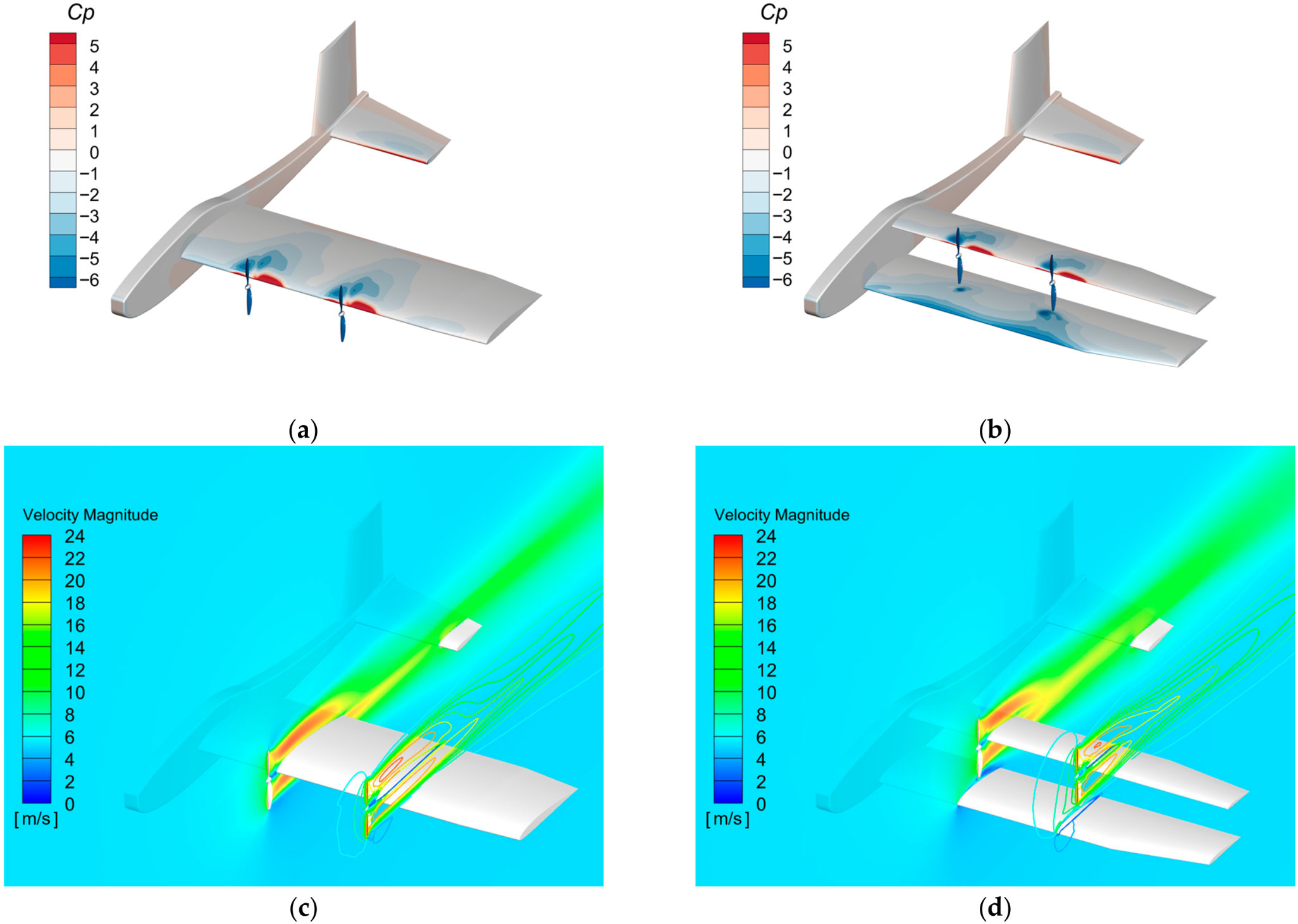
Figure 30 illustrates the interaction at α = 8° using cycle-averaged surface pressure in (a) and (b) and instantaneous velocity at the selected propeller phase in (c) and (d). In CONV, the downstream slipstream acts directly on the wing, concentrating its pressure response in the slipstream-covered region. These pressure patterns qualitatively support the computed change in total airframe loading.

Figure 30. Surface pressure coefficient and propeller-slipstream velocity fields of CONV and PAB at the hand-launch condition with α = 8°: (a) cycle-averaged airframe surface pressure coefficient for CONV; (b) cycle-averaged airframe surface pressure coefficient for PAB; (c) instantaneous velocity magnitude for CONV; (d) instantaneous velocity magnitude for PAB. In (c,d), filled and line contours show the longitudinal planes through the inboard and outboard propeller axes, respectively.

Assuming horizontal release velocity and a mass of 3.0 kg, the 12° lift margins L_total − W are 0.37 N for CONV and 0.68 N for PAB, corresponding to initial vertical accelerations of approximately 0.12 and 0.23 m/s². The approximately 24 N forward resultants correspond to about 8 m/s². These are force balances based on cycle-mean loads at a prescribed release state; a trajectory or pitching response would additionally depend on the evolving aerodynamic state, mass moment of inertia, and control system.

In summary, within the representative angle-of-attack range, PAB provides greater lift per unit shaft power, a comparable positive forward resultant, and a substantially smaller nose-down moment about the respective layout-selected reference CGs.

5. Conclusions

This study examined propeller–wing interactions and the aerodynamic performance of a hand-launched propeller-aided biplane (PAB) UAV with distributed electric propulsion, using a conventional tractor (CONV) reference under common mission requirements and comparable design constraints. The main conclusions are as follows:

(1) Transition modeling considerably affects predicted clean-airframe drag and lift-to-drag ratio. For the powered PAB test case, MRF and sliding-mesh methods produce similar mean propeller thrust but noticeably different mean airframe lift and pitching moment. Sliding-mesh results also reveal periodic wing-pressure redistribution. These findings support accounting for transition and time-dependent propeller–wing interactions when assessing the present UAV.

(2) Among the propeller–wing arrangements examined in the periodic model, OTW produces the largest lift enhancement, while LE-T also provides a significant lift increase. The aerodynamic benefits depend on propeller placement and involve different trade-offs among lift, net streamwise force, and pitching moment. Propeller efficiency alone is insufficient to characterize the installation benefits of the coupled system. Under the conditions in this paper, changes in wing loading are more pronounced than changes in propeller thrust and efficiency.

(3) At cruise, the clean PAB configuration has a lower lift-to-drag ratio than CONV, potentially reflecting its shorter chords, lower Reynolds numbers, and inter-wing interference. Under power, its smaller propeller-induced airframe drag penalty largely offsets this disadvantage.

(4) In the representative hand-launch angle-of-attack range of 8–12°, PAB provides greater total lift and a comparable positive net streamwise force at comparable or slightly lower shaft power. At 12°, its total lift per unit summed propeller shaft power is approximately 4% higher than that of CONV. About the respective design CGs, cycle-mean nose-down moment magnitudes are approximately 77% and 49% smaller for PAB than CONV at 8° and 12°. The pressure and velocity fields suggest complementary interactions of the lower wing with upstream propeller induction and the upper wing with the downstream slipstream. PAB achieves these favorable predicted release-state loads without higher propeller efficiency.

These benefits were obtained without systematic geometric optimization. Refining wing-area distribution and wing–propeller positions may improve the balance among low-speed lift effectiveness, pitching moment, and cruise performance.

References

- Zhou, Y. Unmanned aerial vehicles based low-altitude economy with lifecycle techno-economic-environmental analysis for sustainable and smart cities. J. Clean. Prod. 2025, 499, 145050. [Google Scholar] [CrossRef] [Scilit]
- Oettershagen, P.; Melzer, A.; Mantel, T.; Rudin, K.; Stastny, T.; Wawrzacz, B.; Hinzmann, T.; Leutenegger, S.; Alexis, K.; Siegwart, R. Design of small hand-launched solar-powered UAVs: From concept study to a multi-day world endurance record flight. J. Field Robot. 2017, 34, 1352–1377. [Google Scholar] [CrossRef] [Scilit]
- Mueller, T.J.; DeLaurier, J.D. Aerodynamics of Small Vehicles. Annu. Rev. Fluid Mech. 2003, 35, 89–111. [Google Scholar]
- Abu Salem, K.; Palaia, G.; Bravo-Mosquera, P.D.; Quarta, A.A. A review of novel and non-conventional propulsion integrations for next-generation aircraft. Designs 2024, 8, 20. [Google Scholar] [CrossRef] [Scilit]
- Borer, N.K.; Patterson, M.D.; Viken, J.K.; Moore, M.D.; Clarke, S.; Redifer, M.E.; Christie, R.J.; Stoll, A.M.; Dubois, A.; Bevirt, J.; et al. Design and performance of the NASA SCEPTOR distributed electric propulsion flight demonstrator. In Proceedings of the 16th AIAA Aviation Technology, Integration, and Operations Conference, Washington, DC, USA, 13–17 June 2016. [Google Scholar]
- Keller, D. Towards higher aerodynamic efficiency of propeller-driven aircraft with distributed propulsion. CEAS Aeronaut. J. 2021, 12, 777–791. [Google Scholar] [CrossRef] [Scilit]
- Wang, H.B.; Zhou, Z.; Xu, X.P.; Zhu, X.P. Influence analysis of propeller location parameters on wings using a panel/viscous vortex particle hybrid method. Aeronaut. J. 2018, 122, 21–41. [Google Scholar] [CrossRef] [Scilit]
- Sinnige, T.; van Arnhem, N.; Stokkermans, T.C.A.; Eitelberg, G.; Veldhuis, L.L.M. Wingtip-mounted propellers: Aerodynamic analysis of interaction effects and comparison with conventional layout. J. Aircr. 2019, 56, 295–312. [Google Scholar] [CrossRef] [Scilit]
- Cole, J.A.; Krebs, T.; Barcelos, D.; Bramesfeld, G. Influence of propeller location, diameter, and rotation direction on aerodynamic efficiency. J. Aircr. 2021, 58, 63–71. [Google Scholar] [CrossRef] [Scilit]
- de Vries, R.; Vos, R. Aerodynamic Performance Benefits of over-the-wing distributed propulsion for hybrid-electric transport aircraft. J. Aircr. 2023, 60, 1201–1218. [Google Scholar] [CrossRef] [Scilit]
- Ananda, G.K.; Selig, M.S.; Deters, R.W. Experiments of propeller-induced flow effects on a low-Reynolds-number wing. AIAA J. 2018, 56, 3279–3294. [Google Scholar] [CrossRef] [Scilit]
- de Vries, R.; van Arnhem, N.; Avallone, F.; Ragni, D.; Vos, R.; Eitelberg, G.; Veldhuis, L.L.M. Experimental investigation of over-the-wing propeller-boundary-layer interaction. AIAA J. 2021, 59, 2169–2182. [Google Scholar] [CrossRef] [Scilit]
- Okawa, M.; Nishimura, R.; Ikami, T.; Nagai, H. Unsteady propeller wake interference on wing in tractor configuration at low-Reynolds-number condition. J. Aircr. 2025, 62, 3–12. [Google Scholar] [CrossRef] [Scilit]
- Maqsood, A.; Go, T.H. Parametric studies and performance analysis of a biplane micro air vehicle. Int. J. Aeronaut. Space Sci. 2013, 14, 229–236. [Google Scholar] [CrossRef] [Scilit][Green Version]
- Jones, R.; Cleaver, D.J.; Gursul, I. Aerodynamics of biplane and tandem wings at low Reynolds numbers. Exp. Fluids 2015, 56, 124. [Google Scholar] [CrossRef] [Scilit]
- Wang, H.; Gan, W.; Li, D. An investigation of the aerodynamic performance for a propeller-aided lift-enhancing double wing configuration. Aerosp. Sci. Technol. 2020, 105, 105991. [Google Scholar] [CrossRef] [Scilit]
- Wang, K.; Zhou, Z. An investigation on the aerodynamic performance of a hand-launched solar-powered UAV in flying wing configuration. Aerosp. Sci. Technol. 2022, 129, 107804. [Google Scholar] [CrossRef] [Scilit]
- Wang, H.; Li, G.; Li, J.; Zhuang, J. Aerodynamic investigation for a propeller-induced lift-enhancing vertical take-off and landing (VTOL) configuration. Drones 2025, 9, 20. [Google Scholar] [CrossRef] [Scilit]
- Walters, D.K.; Cokljat, D. A three-equation eddy-viscosity model for Reynolds-averaged Navier-Stokes simulations of transitional flow. J. Fluids Eng. 2008, 130, 121401. [Google Scholar] [CrossRef] [Scilit]
- McAlister, K.W.; Pucci, S.L.; McCroskey, W.J.; Carr, L.W. An Experimental Study of Dynamic Stall on Advanced Airfoil Sections. Volume 2: Pressure and Force Data; NASA-TM-84245-VOL-2; NASA: Washington, DC, USA, 1982. [Google Scholar]
- McCroskey, W.J.; McAlister, K.W.; Carr, L.W.; Pucci, S.L. An Experimental Study of Dynamic Stall on Advanced Airfoil Sections. Volume 1: Summary of the Experiment; NASA-TM-84245-VOL-1; NASA: Washington, DC, USA, 1982. [Google Scholar]
- Gall, P.D.; Smith, H.C. Aerodynamic characteristics of biplanes with winglets. J. Aircr. 1987, 24, 518–522. [Google Scholar] [CrossRef] [Scilit] [PubMed]
- Li, X. Research on Efficient Calculation Method of Distributed Propulsion/Wing Coupling and Lift Augmentation Design. Ph.D. Thesis, Northwestern Polytechnical University, Xi’an, China, 2025. [Google Scholar]
- Jones, B. Elements of Practical Aerodynamics, 4th ed.; Wiley: New York, NY, USA, 1950. [Google Scholar]
Disclaimer/Publisher’s Note: The statements, opinions and data contained in all publications are solely those of the individual author(s) and contributor(s) and not of MDPI and/or the editor(s). MDPI and/or the editor(s) disclaim responsibility for any injury to people or property resulting from any ideas, methods, instructions or products referred to in the content. |
© 2026 by the authors. Licensee MDPI, Basel, Switzerland. This article is an open access article distributed under the terms and conditions of the Creative Commons Attribution (CC BY) license.