Memory-Dependent Derivative Versus Fractional Derivative (III): Difference in Modeling Epidemics

Abstract

The outbreaks of large-scale epidemics, such as COVID-19 in 2019–2022, challenge modelers. Beside the effect of the incubation period of the virus, the delay property of detection should be also stressed. This kind of memory effect affects the entire change rate, which cannot be reflected by the conventional instantaneous derivative. The fractional derivative (FD) meets this request to some extent. Yet the shortcoming of it limits its usage. Through a strict modeling approach, a new susceptible–infective–removed (SIR) model with the memory-dependent derivative (MDD) has been constructed. The numerical simulations indicate that (1) the neglecting of the incubation period may underestimate the number of susceptible individuals and overestimate the infected ones; (2) the neglecting of the treatment period may badly overestimate the removed individuals; (3) the consequence of tardy detection intervention may be very serious, and the infectious rate may increase rapidly with a postponed peak time; and (4) the SIR model with the FD yields bad estimations, not only in the primary stage but also in the subsequent evolution. Due to the reasonability of the new SIR model with the MDD, it is suggested to epidemic researchers.

1. Introduction

The outbreak of a novel coronavirus disease from 2019 to 2022 (COVID-19) has challenged all the related scientists around the world. What applied mathematicians can do is conduct modeling with respect to the spread of this pandemic. Though it has passed, carrying out modeling research is still meaningful for other possible epidemics. Among all the existing models, direct application in [1,2,3,4] and extended application in [5,6,7], simple or complex, most of them start from the susceptible–infective–removed (SIR) model, which was constructed by Kermack and McKendrick in 1927 [8]. So the SIR model can be taken as the base for any improvements. Here we stress the “memory effect” and reconstruct this model by adopting a strict modeling approach. Coincidentally, the reconstructed one has a change rate in the form of the “memory-dependent derivative (MDD)”, which accords with the studies in [9,10,11].

As far as the COVID-19 pandemic is concerned, letting it spread freely is impossible. The preventions and control interventions from the governments should be stressed in the remodeling. There are five non-negligible factors for this pandemic; these are the vaccination campaign, the nucleic acid detection, the tracing of close contacts, the asymptomatic individuals, and fatality. Hence, before considering the memory effect, the meanings of the three compartments need to be restated. We note that adding compartments is not a good strategy. In fact, the asymptomatic individuals are the virus carriers and the vaccinated individuals can still get the virus and infect others. Since the coronavirus updates frequently, vaccination does not mean the gaining of long-term immunity; it can only relieve the symptoms in case an individual is infected. The other three factors are associated with the memory effect.

Before the widespread adoption of nucleic acid detection, the main approach was to diagnose with the symptoms. At this stage, the incubation period (the time after exposure to the virus until symptom onset) was non-negligible. According to the review in [12], the average incubation period is 5 to 6 days (up to 14 days), and the suggested quarantine period is set as 1 to 2 weeks. The “incubation period” can be re-understood as the time after exposure to the virus until the individual becomes a medium and infects others. In mathematical language, the change rate of the infected number I at moment t is not merely the instantaneous change rate $dI/dt$, and it should be in the form of the weighted mean of $dI/ds$ over a certain interval, such as $[t-\tau ,t]$, with respect to the argument s. Here $\tau$ accords with the average waiting period from the infected moment to definite diagnosis. We note that this memory effect cannot be fully reflected by simply incorporating a retarded term $I(t-\tau )$, since the average period of definite diagnosis is the expected value of a distribution, which complicates the change rate.

There have been many attempts to reflect the memory effect of the COVID-19 pandemic, such as in [13,14,15,16,17] for epidemic models, in [18,19,20,21,22] for expand researches and [23,24,25,26] for analysis researches. Their common point lies in borrowing the “fractional derivative (FD)” [27,28,29]. However, just as indicated in [30,31], to generalize the dynamic models with the FD, the scientific principles should be obeyed. Before constructing a new model, the physical meaning of the derivative for a certain dynamic system should be clarified. In fact, from the analyses in [9,10] we see that, as far as the memory effect is concerned, the shortcomings of the FD are quite clear. The reasonability is hard to guarantee for the application of it to the COVID-19 pandemic.

Specifically speaking, let m be a positive integer and $\alpha$ be a fraction with $m-1<\alpha \le m$; then the representative definition of the fractional derivative is as follows [27,28,29].

Definition 1. 

If the m-order common derivative of $f\left(t\right)$ [that is, $f^{\left(m\right)}\left(t\right)$] exists, then

$$\begin{array}{c}\hfill D_t^{\alpha }f\left(t\right)={\displaystyle \frac{1}{\mathsf{\Gamma }(m-\alpha )}}{\int }_{t_0}^t{K}_{\alpha }(t-s)f^{\left(m\right)}\left(s\right)ds\end{array}$$

(1)

is called the α-order Caputo type of the fractional derivative (FD) of $f\left(t\right)$, where

$$\begin{array}{c}\hfill \mathsf{\Gamma }(m-\alpha )={\int }_0^{\infty }{x}^{m-\alpha -1}{e}^{-x}dx,K_{\alpha }(t-s)={\displaystyle \frac{1}{{(t-s)}^{\alpha +1-m}}}\end{array}$$

(2)

and $t_0$ is a fixed reference moment.

Relatively, the memory-dependent derivative is defined as follows [9,10,11].

Definition 2. 

If the m-order common derivative of $f\left(t\right)$ [that is, $f^{\left(m\right)}\left(t\right)$] exists, then

$$\begin{array}{c}\hfill D_{t,\tau }^{m}f\left(t\right)={\displaystyle \frac{1}{\tau }}{\int }_{t-\tau }^{t}K(t-s)f^{\left(m\right)}\left(s\right)ds\end{array}$$

(3)

is called the m-order memory-dependent derivative (MDD) of $f\left(t\right)$, relative to the time delay $\tau (>0)$ and weighted function $K(t-s)$, which is m-times differentiable with respect to t and s.

From the above definitions we see these two derivatives have the same form. They are both defined as some weighted mean of the common integer-order derivative. They differ in the following aspects [9,10]:

(I)

The integral interval of the FD is $[t_0,t]$, which becomes wider and wider along with the increasing of t. This characteristic does not match the memory effect of the COVID-19 pandemic, since its incubation period is finite (no longer than 14 days; the average time is 5 to 6 days, see [12]). Yet, the MDD is defined on a slipping interval $[t-\tau ,t]$, which maintains its width, and this matches the above fact.

(II)

The weighted function $K_{\alpha }(t-s)$ for the FD is fixed, yet that for the MDD can be chosen freely. For example, as indicated in [10],

$$\begin{array}{c}\hfill {\left({\displaystyle \frac{\tau +s-t}{\tau }}\right)}^{\sigma },sin\left[{\displaystyle \frac{(\tau +s-t)\pi }{2\tau }}\right],{\displaystyle \frac{(t-s+\tau )(s-t+\tau ))}{{\tau }^2}}\end{array}$$

with $\sigma >0$ being all the permitted forms of $K(t-s)$. This freedom of choice enables the remodeling of many different dynamic processes with the MDD.

(III)

There is the fact that $K_{\alpha }(t-s)=1/{(t-s)}^{\alpha +1-m}\to \infty$ as $s\to t$. This implies that the instantaneous change rate at $s=t$ is amplified with a ∞ weight, and the FD mainly reflects the local change, though it is defined in a non-local form. Yet, the MDD is a real non-local one, except for the particular case $K(t-s)\equiv 1$, which accords with the common derivative as $\tau \to 0$. The basic requirements below [9,10]

$$\begin{array}{c}\hfill {K(t-s)|}_{s=t-\tau }{=0,K(t-s)|}_{s=t}=1\end{array}$$

ensure that the weighted function has a finite variation, and outside the slipping interval $[t-\tau ,t]$ there is no memory effect.

Based on the above analyses, we see that the MDD is much better than the FD in reflecting the memory effect. But, the direct usage of the MDD in modeling is not suggested. We agree with the remarks in [30,31], and the scientific principles should be obeyed. With respect to the memory effect of the COVID-19 pandemic, in the following section we will reconstruct a new SIR model for it by adopting a strict modeling approach. Numerical algorithms and related simulations are given in Section 3. In addition, the conclusions are given in the last section.

2. Reconstructing SIR Model with Memory Effect

The conventional SIR model given by Kermack and McKendrick in 1927 is as follows [1,4,5,8]:

$$\begin{array}{ccc}& & S^{\prime }\left(t\right)=-\beta S\left(t\right)I\left(t\right),\hfill \end{array}$$

(4)

$$\begin{array}{ccc}& & I^{\prime }\left(t\right)=\beta S\left(t\right)I\left(t\right)-\gamma I\left(t\right),\hfill \end{array}$$

(5)

$$\begin{array}{ccc}& & R^{\prime }\left(t\right)=\gamma I\left(t\right).\hfill \end{array}$$

(6)

Here the denotation “$\prime$” means the taking of the common derivative. $S\left(t\right)$, $I\left(t\right)$, and $R\left(t\right)$ are the numbers of susceptible, infected, and removed individuals at time t, respectively. The constant $\beta$ is the transition rate between $S\left(t\right)$ and $I\left(t\right)$. $\gamma$ is the transition rate between $I\left(t\right)$ and $R\left(t\right)$. There is a fundamental hypothesis for this compartmentalized model that the total population over the duration of the epidemic remains unchanged, say N, and the relation

$$\begin{array}{c}\hfill S\left(t\right)+I\left(t\right)+R\left(t\right)=N\end{array}$$

(7)

holds true. We note that, for simplicity of calculation, Equation (6) can be substituted by this relation.

Referring to the descriptions in [1,6], the above three compartments can be restated as follows:

• $S\left(t\right)$ is the number of susceptible individuals, which includes the vaccinated ones and those that are not infected by the disease (not the virus carriers);
• $I\left(t\right)$ is the number of infected individuals, which includes the asymptomatic ones (all the virus carriers);
• $R\left(t\right)$ is the number of individuals who can no longer be infected, either because they recovered and gained long-term immunity or because they passed away (in case the recovered individuals have close contact with the infected ones again, the virus has no effect on them and it is almost impossible for them to become mediums and infect others).

In addition, as far as fatality is concerned, it needs no additional compartment. The number of deaths can be simply calculated by $\delta R\left(t\right)$, where $\delta$ is a proportionality coefficient.

In the following we start by considering the variation in the infected by adopting a rigid modeling approach, as in [10,11].

2.1. Modifying the Infected Equation

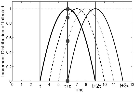
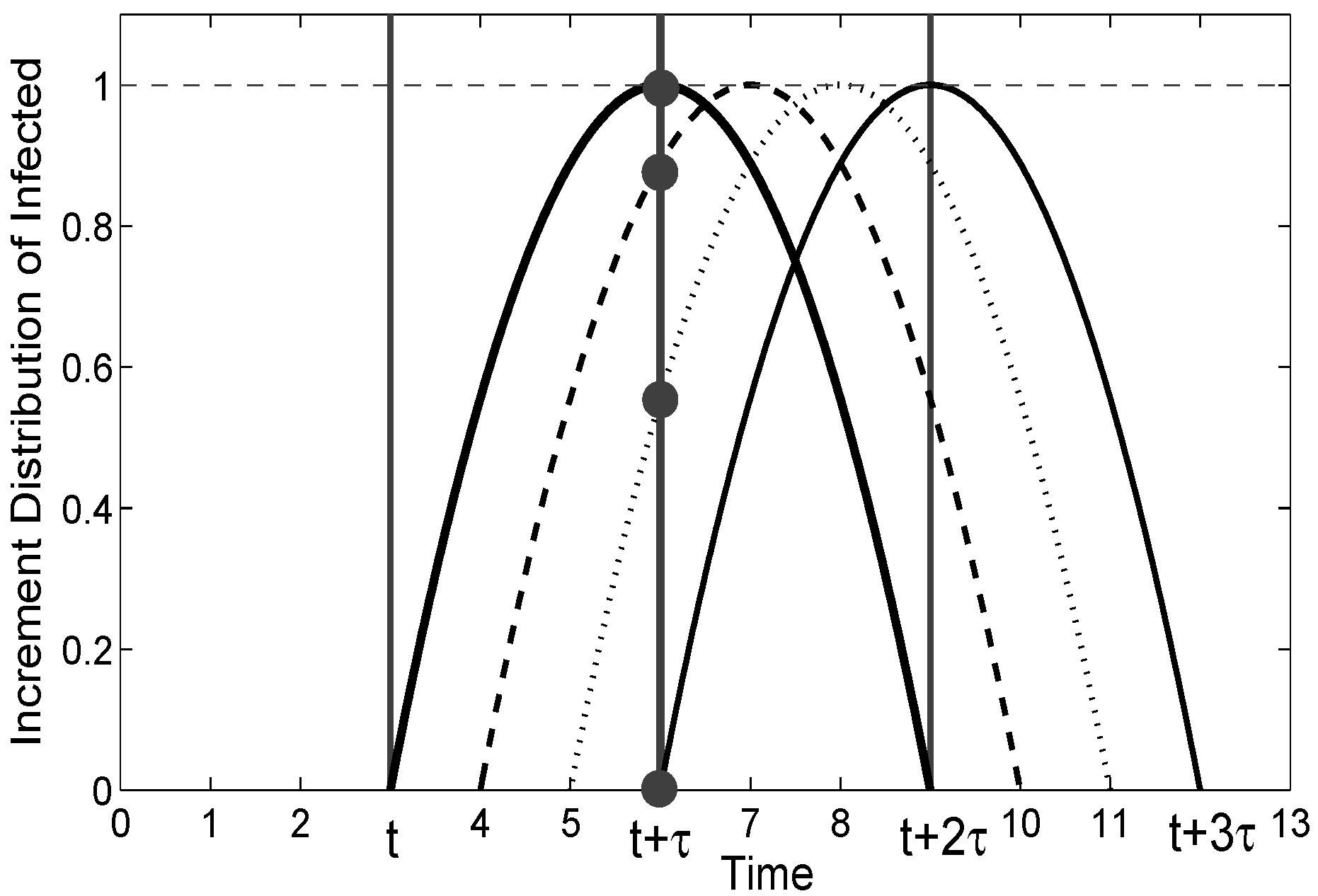
According to the analyses in the previous section, the average period of definite diagnosis (waiting from the infected moment), denoted by $\tau$, is the expected value of a distribution. The change rate of $I\left(t\right)$ should rely on this distribution and the derivative needs to be modified. Objectively speaking, obtaining the distribution law requires a detailed medical investigation. But this is not available for us now. Notice that most of the conventional processes obey the Normal distribution in statistics; we continue the theoretical study by assuming that the distribution function is symmetric, as in Figure 1.

Figure 1. A possible distribution of the infection increment over time s; here the distribution function is chosen as $(s-t+\tau )(t-s+\tau )/{\tau }^2$, with $\tau =3$. Different curves correspond to the same distribution with different locations.

To trace back, the original discrete form of Equation (5) reads

$$\begin{array}{c}\hfill I(t+▵t)-I\left(t\right)=\left[\beta S\right(t)-\gamma ]I\left(t\right)▵t,\end{array}$$

(8)

where $▵t$ is a small time segment. Considering the total increment on $[t,t+\tau ]$, this equation needs to be modified. We note that here and in the following, t is always taken as the default reference moment.

We follow the processing approach in [11] and divide $\tau$ into n equal parts with $▵t$; that is, $n▵t=\tau$. According to the assumption on the distribution, the infected individuals on $[t-▵t/2,t+▵t/2]$, as infection sources, infect others and result in new increments on $[t,t+2\tau ]$. Let $I_i$ be the number of infected at $t_i=t+i▵t$, with $0\le i\le 2n$. In fact, the infected individuals on $[t-▵t/2,t+▵t/2]$ only contribute partially to the infection increment $▵I_i=I_i-I_{i-1}$, and the other parts should contribute to the infected individuals on the other time segments. To be explicit, we denote $▵u_{i,j}$ as the number of new infected individuals on $[t_{i-1},t_i]$ who were infected by the ones who were already virus carriers on $[t_{j-1},t_j]$.

With respect to the infection sources (the already infected individuals) on $[t-▵t/2,t+▵t/2]$, the total number of infection increments on $[t,t+2\tau ]$ reads

$$▵U_1=\sum _{i=1}^{2n}▵u_{i,1}.$$

(9)

Similarly, for an arbitrary integer m with $2\le m\le n$, the infection sources on $[t+(m-1/2)▵t,t+(m+1/2)▵t]$ result in an increment:

$$▵U_m=\sum _{i=m}^{2n+m-1}▵u_{i,m}.$$

(10)

Hence, with respect to all the infection sources (all the individuals who were already infected) on $[t,t+\tau ]$, the total number of newly infected ones reads

$$\begin{array}{ccc}\hfill U_{all}& =& \sum _{m=1}^n▵U_m=\sum _{m=1}^n\sum _{i=m}^{2n+m-1}▵u_{i,m}\hfill \\ \hfill & =& \sum _{m=1}^n\left[\sum _{i=m}^n+\sum _{i=n+1}^{n+m-1}+\sum _{i=n+m}^{2n}+\sum _{i=2n+1}^{2n+m-1}\right]▵u_{i,m}\hfill \\ \hfill & =& {\lambda }_n\sum _{m=1}^n\sum _{i=m}^n▵u_{i,m}={\lambda }_n\sum _{m=1}^n{K}_m▵I_m\hfill \\ \hfill & =& {\lambda }_n\sum _{m=1}^n{K}_m{\displaystyle \frac{▵I_m}{▵t}}▵t,\hfill \end{array}$$

(11)

where ${\lambda }_n$ and $K_m$ are the scale factors.

It follows from the symmetric assumption on the distribution function (see Figure 1) that

$$\begin{array}{ccc}& & \sum _{m=1}^n\sum _{i=2n+1}^{2n+m-1}▵u_{i,m}=\sum _{m=1}^n\sum _{i=m}^n▵u_{i,m},\hfill \\ & & \sum _{m=1}^n\sum _{i=n+m}^{2n}▵u_{i,m}>\sum _{m=1}^n\sum _{i=m}^n▵u_{i,m},\hfill \\ & & \sum _{m=1}^n\sum _{i=n+1}^{n+m-1}▵u_{i,m}>\sum _{m=1}^n\sum _{i=m}^n▵u_{i,m}.\hfill \end{array}$$

These indicate that ${\lambda }_n>4$. In view of the fact that the the summation is finite and the limit exists as $n\to \infty$, we have ${\lambda }_n\to \lambda$ with $\lambda >4$.

According to Equation (11), the already infected individuals on $[t+(m-1/2)▵t,t+(m+1/2)▵t]$ infect new ones, and the total number of them on $[t+(m+1/2)▵t,t+(n+1/2)▵t]$ is expressed in the form of $K_m▵I_m=K_m(I_m-I_{m-1})$. Notice that $▵I_m$ is an entire increment that has a relatively large magnitude; in all probability the factor $K_m$ acts as a proportionality coefficient with $0<K_m\le 1$.

Let $▵t\to 0$; then $n\to \infty$ accordingly ($n▵t=\tau$ is fixed), and it follows from Equation (11) that

$$\begin{array}{c}\hfill U_{all}\to \lambda {\int }_t^{t+\tau }K(s-t)I^{\prime }\left(s\right)ds,\end{array}$$

(12)

where $K(s-t)$ is a continuous function defined on the slipping interval $[t,t+\tau ]$. It can be seen as a continuous extension of $K_1,K_2,\cdots K_n$ as $n\to \infty$.

The quantity in Equation (12) is the entire increment of the infected individuals on the time segment $[t,t+\tau ]$. For this case, Equation (8) can be modified as

$$\begin{array}{c}\hfill \lambda {\int }_t^{t+\tau }K(s-t)I^{\prime }\left(s\right)ds=[\beta S\left(t\right)-\gamma ]I\left(t\right)\tau .\end{array}$$

(13)

Substituting $\lambda$ by ${\lambda }_2$, $K(s-t)$ by $K_2(s-t)$, and $\tau$ by ${\tau }_2$ results in the final form of the infected equation:

$$\begin{array}{c}\hfill {\lambda }_2{D}_{t,{\tau }_2}I\left(t\right)=[\beta S\left(t\right)-\gamma ]I\left(t\right)\end{array}$$

(14)

with ${\lambda }_2>4$ and

$$\begin{array}{c}\hfill D_{t,{\tau }_2}I\left(t\right)={\displaystyle \frac{1}{{\tau }_2}}{\int }_t^{t+{\tau }_2}{K}_2(s-t)I^{\prime }\left(s\right)ds,\end{array}$$

(15)

which, coincidentally, accords with the “memory-dependent derivative (MDD)” defined in Definition 2. To be a formal form of the MDD, one only needs to rewrite $K_2(s-t)$ into $K_2(t+{\tau }_2-s)$ and substitute t by $t-{\tau }_2$. The forward form of the MDD in Equation (15) can simplify the right expression in Equation (14) and is adopted here.

2.2. New SIR Model with MDD

Notice that ${\tau }_2$ is the average period of definite diagnosis (waiting from the infected moment); we use ${\tau }_1$ and ${\tau }_3$ to denote the average tracing period of close contacts (which is always performed after an individual is diagnosed) and the average treatment period for the recovered and deceased individuals, respectively.

Repeating the modeling process in the previous section, we obtain similar equations for the susceptible and removed ones. The new SIR model with the MDD is as follows:

$$\begin{array}{ccc}& & {\lambda }_1{D}_{t,{\tau }_1}S\left(t\right)=-\beta S\left(t\right)I\left(t\right),\hfill \end{array}$$

(16)

$$\begin{array}{ccc}& & {\lambda }_2{D}_{t,{\tau }_2}I\left(t\right)=[\beta S\left(t\right)-\gamma ]I\left(t\right),\hfill \end{array}$$

(17)

$$\begin{array}{ccc}& & {\lambda }_3{D}_{t,{\tau }_3}R\left(t\right)=\gamma I\left(t\right).\hfill \end{array}$$

(18)

with ${\lambda }_1,{\lambda }_2,{\lambda }_3>4$ and

$$\begin{array}{ccc}& & D_{t,{\tau }_1}S\left(t\right)={\displaystyle \frac{1}{{\tau }_1}}{\int }_t^{t+{\tau }_1}{K}_1(s-t)S^{\prime }\left(s\right)ds,\hfill \end{array}$$

(19)

$$\begin{array}{ccc}& & D_{t,{\tau }_2}I\left(t\right)={\displaystyle \frac{1}{{\tau }_2}}{\int }_t^{t+{\tau }_2}{K}_2(s-t)I^{\prime }\left(s\right)ds,\hfill \end{array}$$

(20)

$$\begin{array}{ccc}& & D_{t,{\tau }_3}R\left(t\right)={\displaystyle \frac{1}{{\tau }_3}}{\int }_t^{t+{\tau }_3}{K}_3(s-t)R^{\prime }\left(s\right)ds,\hfill \end{array}$$

(21)

where the weighted functions satisfy the limitations below:

$$\begin{array}{c}\hfill K_i(s-t){{|}_{s=t}=0,K_i(s-t)|}_{s=t+{\tau }_i}=1,i=1,2,3.\end{array}$$

We note that the scale factor ${\lambda }_i(>4)$ may be related to the weighted function $K_i(s-t)$. But the exact relationship between them is unknown. This is left as an open problem.

Adding Equations (16)–(18) leads to

$$\begin{array}{c}\hfill {\lambda }_1{D}_{t,{\tau }_1}S\left(t\right)+{\lambda }_2{D}_{t,{\tau }_2}I\left(t\right)+{\lambda }_3{D}_{t,{\tau }_3}R\left(t\right)=0.\end{array}$$

(22)

which does not imply $S\left(t\right)+I\left(t\right)+R\left(t\right)=N$. It only indicates that for an arbitrary moment t the entire change rate is 0.

3. Numerical Simulations

In the following we investigate the variation of SIR model caused by the memory effect. In particular, the influences of different delays and weighted functions are stressed.

As far as the MDD is concerned, the difficulty in numerical simulation lies in processing the integral on the slipping interval. In [10] we developed a universal algorithm for this with the well-known Simpson formula, and it can be borrowed for our present problem. To accord with this algorithm, we rewrite $K_i(s-t)$ into ${\overline{K}}_i(t+{\tau }_i-s)$. Furthermore, we substitute t by $t-{\tau }_i$ and $S\left(t\right)$, $I\left(t\right)$, and $R\left(t\right)$ by $NS\left(t\right)$, $NI\left(t\right)$, and $NR\left(t\right)$; then the normalized new SIR model with the MDD in (16)–(18) can be rewritten as follows:

$$\begin{array}{ccc}& & {\lambda }_1{D}_{t,{\tau }_1}S\left(t\right)=-{\beta }_{0}S(t-{\tau }_1)I(t-{\tau }_1),\hfill \end{array}$$

(23)

$$\begin{array}{ccc}& & {\lambda }_2{D}_{t,{\tau }_2}I\left(t\right)=[{\beta }_{0}S(t-{\tau }_2)-\gamma ]I(t-{\tau }_2),\hfill \end{array}$$

(24)

$$\begin{array}{ccc}& & {\lambda }_3{D}_{t,{\tau }_3}R\left(t\right)=\gamma I(t-{\tau }_3)\hfill \end{array}$$

(25)

with ${\beta }_0=\beta N$. In case the nucleic acid detection is performed for all, no tracing of the close contacts is needed, and there are ${\lambda }_1={\lambda }_2$, ${\tau }_1={\tau }_2$, and ${\overline{K}}_1(t+{\tau }_1-s)={\overline{K}}_2(t+{\tau }_2-s)$. As far as the memory effect is concerned, this simple case is suitable for our consideration.

The united form of Equations (23)–(25) is as follows:

$$\begin{array}{c}\hfill {\displaystyle \frac{\lambda }{\tau }}{\int }_{t-\tau }^t\overline{K}(t-s)u^{\prime }\left(s\right)ds=f(t-\tau ).\end{array}$$

(26)

Here the variable u stands for the normalized $S,I$, or R. $f(t-\tau )$ stands for one of the following expressions:

$$\begin{array}{c}\hfill -{\beta }_{0}S(t-\tau )I(t-\tau ),[{\beta }_{0}S(t-\tau )-\gamma ]I(t-\tau ),\gamma I(t-\tau ).\end{array}$$

Comparatively, the normalized conventional SIR model in Equations (4) and (5) is as follows:

$$\begin{array}{ccc}& & S^{\prime }\left(t\right)=-{\beta }_{0}S\left(t\right)I\left(t\right),\hfill \end{array}$$

(27)

$$\begin{array}{ccc}& & I^{\prime }\left(t\right)={\beta }_{0}S\left(t\right)I\left(t\right)-\gamma I\left(t\right),\hfill \end{array}$$

(28)

$$\begin{array}{ccc}& & R^{\prime }\left(t\right)=\gamma I\left(t\right).\hfill \end{array}$$

(29)

For their numerical simulations, the simple difference scheme $u_k=u_{k-1}+h{f}_{k-1}$ can be adopted, where h is understood as the time-step.

In dealing with the MDD, the following transform is adopted:

$$\begin{array}{c}\hfill {\int }_{t-\tau }^t\overline{K}(t-s)u^{\prime }\left(s\right)ds=u\left(t\right)-{\int }_{t-\tau }^t{\displaystyle \frac{\partial \overline{K}}{\partial s}}u\left(s\right)ds.\end{array}$$

where the limitations $\overline{K}\left(\tau \right)=0$ and $\overline{K}\left(0\right)=1$ are used.

Let n be a positive integer; we divide the interval $[-\tau ,0]$ with h into $2n$ parts; that is $\tau =2nh$. We denote $t_k=(k-1)h-\tau$, $u_k=u\left(t_k\right)$, $f_{k-2n}=f(t_k-\tau )$ and $P_j=P(t_k-t_{k-2n+j})$ with $P(t-s)=\partial \overline{K}(t-s)/\partial s$ (it is defined on the slipping interval $[t-\tau ,t]$ and does not depend on the location of t); then for $k\ge 2n+1$ the numerical algorithm for Equation (26) reads

$$\begin{array}{c}\hfill u_k={\displaystyle \frac{h}{3-h}}\left[\sum _{i=1}^{n-1}{G}_{k,i}+P_{2n-2}{u}_{k-2}+4P_{2n-1}{u}_{k-1}\right]+{\displaystyle \frac{3\tau }{(3-h)\lambda }}{f}_{k-2n}\end{array}$$

(30)

with $G_{k,i}=P_{2i-2}{u}_{k+2(i-n)-2}+4P_{2i-1}{u}_{k+2(i-n)-1}+P_{2i}{u}_{k+2(i-n)}$. The numerical simulation can be performed by assigning initial conditions on $[-\tau ,0]$. Here we set $S\left(t\right)=0.95e^{-0.01t}$, $I\left(t\right)=1-S\left(t\right)$, and $R\left(t\right)=0$ on this interval.

To perform the simulation, here we choose

$$\begin{array}{c}\hfill \overline{K}(t-s)={\left({\displaystyle \frac{\tau +s-t}{\tau }}\right)}^{\sigma }\end{array}$$

(31)

for the three equations. Notice that

$$P(t-s)={\displaystyle \frac{\partial \overline{K}(t-s)}{\partial s}}={\displaystyle \frac{\sigma }{{\tau }^{\sigma }}}{(\tau +s-t)}^{\sigma -1},$$

and only the cases with $\sigma \ge 1$ are considered.

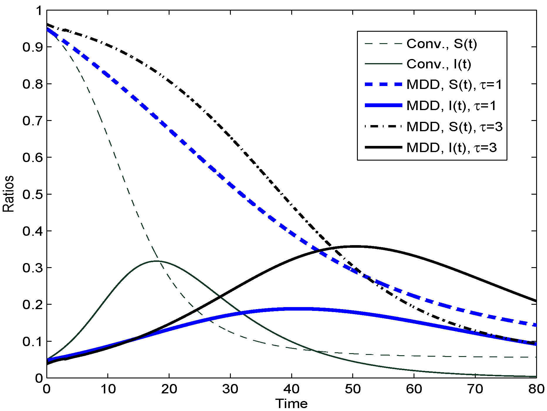
It follows from Figure 2 that the following hold:

(i) 

Relative to the conventional SIR model, the new one with the MDD gives a much slower decreasing curve for $S\left(t\right)$. On the one hand, the neglecting of the incubation period may underestimate the number of susceptible individuals and overestimate the infected ones; on the other hand, the tardy detection intervention (which includes the tracing of close contacts) may overestimate the number of susceptible individuals and underestimate the infected ones.

(ii) 

The consequence of the tardy detection intervention is very serious. The infectious ratio may increase rapidly and its peak time may be also postponed.

In this sense, the evolutions of $S\left(t\right)$ and $I\left(t\right)$ given by the MDD model with $\tau =1$ can be seen as rational results. Those with the case $\tau =3$ can be seen as objective states under governments’ preventions and control interventions.

Figure 2. The effect of time delay $\tau$ on the evolutions of $S\left(t\right)$ and $I\left(t\right)$ given by the normalized new SIR model with the MDD. The corresponding parameters are chosen as ${\beta }_0=0.3$, $\gamma =0.1$, $\lambda =5$, $h=0.01$, and $\sigma =1$.

Figure 2. The effect of time delay $\tau$ on the evolutions of $S\left(t\right)$ and $I\left(t\right)$ given by the normalized new SIR model with the MDD. The corresponding parameters are chosen as ${\beta }_0=0.3$, $\gamma =0.1$, $\lambda =5$, $h=0.01$, and $\sigma =1$.

There is also the fact that the remarkable difference between the MDD model and the conventional model lies in the magnitude of the derivatives. In case $S^{\prime }\left(t\right)$ remains unchanged, say $S^{\prime }\left(t\right)\equiv C$, then

$$\begin{array}{c}\hfill \lambda D_{t,\tau }S\left(t\right)={\displaystyle \frac{\lambda }{\tau }}{\int }_{t-\tau }^t{\left({\displaystyle \frac{\tau +s-t}{\tau }}\right)}^{\sigma }{S}^{\prime }\left(s\right)ds={\displaystyle \frac{\lambda }{\sigma +1}}C,\end{array}$$

which has a bigger magnitude, provided that $\lambda /(\sigma +1)>1$. For example, for the case in Figure 2 with $\lambda =5$ and $\sigma =1$, the total change rate of the MDD model is $2.5$ times that of the conventional one.

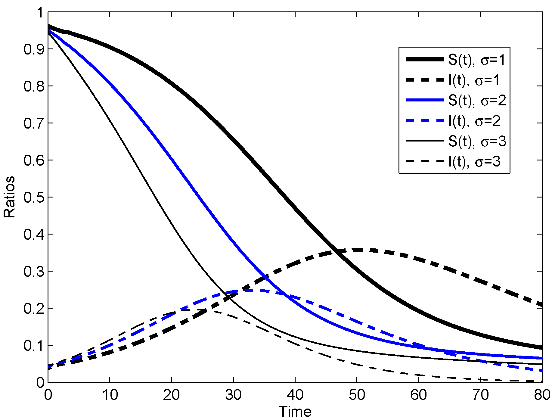
Besides the time delay $\tau$, the weighted function $\overline{K}(t-s)$ also has an effect on the evolutions of $S\left(t\right)$ and $I\left(t\right)$. From Figure 3 we see that, along with the increasing of power $\sigma$ in Equation (31) (that is, the relative weight at $s=t$ gets bigger and bigger), the memory effect may become weaker and weaker. Conversely, the smaller $\sigma$ implies a more serious infection with a postponed peak time.

Figure 3. The effect of the weighted function $\overline{K}(t-s)$ on the evolutions of $S\left(t\right)$ and $I\left(t\right)$ given by the normalized new SIR model with the MDD. The corresponding parameters are chosen as ${\beta }_0=0.3$, $\gamma =0.1$, $\lambda =5$, $h=0.01$, and $\tau =3$.

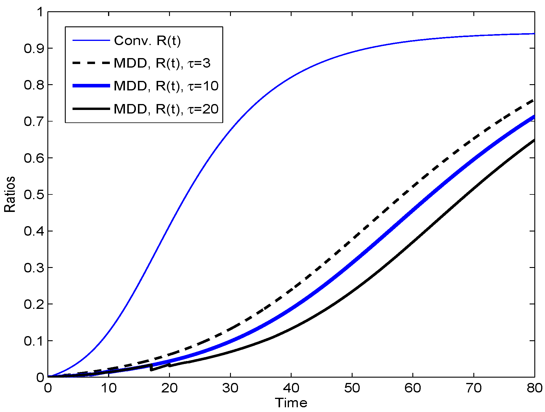
Figure 4 indicates that the effect of treatment period cannot be ignored. The neglecting of it may badly overestimate the removed individuals. Incorporating the MDD can reflect the medical level. On the condition that the medical level is high, the infected individuals receive prompt medical treatment and the recovering period may become short. On the contrary, things may get bad and the death rate may increase. We note that here the delay $\tau$ is actually ${\tau }_3$, which differs from the previous one, say ${\tau }_1=3$. In case ${\tau }_3>{\tau }_1$, the initial conditions $S\left(t\right)=0.95e^{-0.01t}$, $I\left(t\right)=1-S\left(t\right)$ and $R\left(t\right)=0$ are assigned on $[-{\tau }_1,0]$. On another part $[0,{\tau }_3-{\tau }_1]$, we use $R\left(t\right)=1-S\left(t\right)-I\left(t\right)$ to calculate the initial values, since on this interval the values of $S\left(t\right)$ and $I\left(t\right)$ are already calculated.

Figure 4. The effect of time delay $\tau$ on the evolution of $R\left(t\right)$ given by the normalized new SIR model with the MDD. The corresponding parameters are chosen as ${\beta }_0=0.3$, $\gamma =0.1$, $\lambda =5$, $h=0.01$, and $\sigma =1$.

In addition, to make a comparison the normalized SIR model with the FD is also considered. Its explicit equations are

$$\begin{array}{ccc}& & D_t^{\alpha }S\left(t\right)=-{\beta }_{0}S\left(t\right)I\left(t\right),\hfill \end{array}$$

(32)

$$\begin{array}{ccc}& & D_t^{\alpha }I\left(t\right)=[{\beta }_{0}S\left(t\right)-\gamma ]I\left(t\right),\hfill \end{array}$$

(33)

$$\begin{array}{ccc}& & D_t^{\alpha }R\left(t\right)=\gamma I\left(t\right)\hfill \end{array}$$

(34)

with ${\beta }_0=\beta N$, $0<\alpha <1$, and

$$\begin{array}{c}\hfill D_t^{\alpha }u\left(t\right)={\displaystyle \frac{1}{\mathsf{\Gamma }(1-\alpha )}}{\int }_0^t{\displaystyle \frac{1}{{(t-s)}^{\alpha }}}{u}^{\prime }\left(s\right)ds,\end{array}$$

(35)

where the reference moment is chosen as $t_0=0$. The corresponding numerical algorithm is as follows (see [10]):

$$\begin{array}{c}\hfill u_k=h^{\alpha }{f}_{k-1}-\sum _{i=2}^k{g}_i{u}_{k-i+1},\end{array}$$

(36)

where $t_k=(k-1)h$, $u_{k-i+1}=u\left(t_{k-i+1}\right)$, $f_{k-1}=f\left(t_{k-1}\right)$, $g_1=1$, and $g_i=[1-(\alpha +1)/(i-1)]g_{i-1}$ for $i\ge 2$. One only needs to assign an initial condition at $t=0$. Here we choose $S\left(0\right)=0.95$.

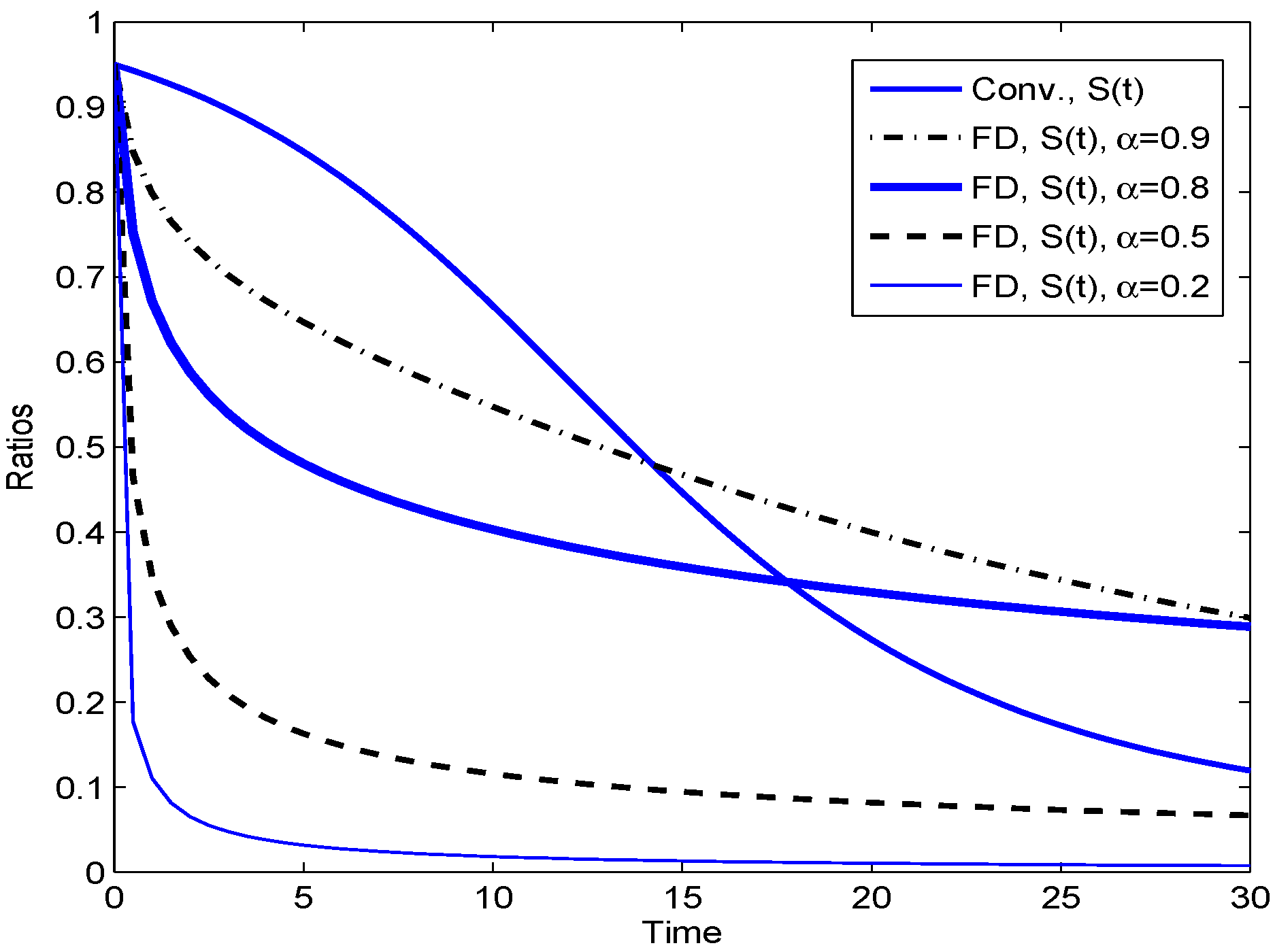
It follows from Figure 5 that, relative to the conventional SIR model, the one with the FD badly underestimates the number of the susceptible individuals at the primary stage, though it differs in degree for different $\alpha$. Yet, conversely, its subsequent evolution seems too flat. This shortcoming of the fractional-order derivative is inherent. The magnitude of this derivative relies on the location of t. Explicitly, in case $S^{\prime }\left(t\right)$ remains unchanged, say $S^{\prime }\left(t\right)\equiv C$, then

$$\begin{array}{c}\hfill D_t^{\alpha }S\left(t\right)={\displaystyle \frac{1}{\mathsf{\Gamma }(1-\alpha )}}{\int }_0^t{\displaystyle \frac{1}{{(t-s)}^{\alpha }}}{S}^{\prime }\left(s\right)ds={\displaystyle \frac{t^{1-\alpha }}{\mathsf{\Gamma }(2-\alpha )}}C.\end{array}$$

That is to say, when t is near the reference point $s=0$, $t^{1-\alpha }/\mathsf{\Gamma }(2-\alpha )$ becomes very small; this is equivalent to zooming in on the right hand $-{\beta }_{0}S\left(t\right)I\left(t\right)$ many times. So, the occurrence of rapid decreasing near $t=0$ in Figure 5 is not strange. Yet, conversely, when t becomes bigger and bigger, $t^{1-\alpha }/\mathsf{\Gamma }(2-\alpha )$ increases accordingly, and a minification occurs on $-{\beta }_{0}S\left(t\right)I\left(t\right)$. This is why the change slows down.

Figure 5. The effect of fractional-order $\alpha$ on the evolution of $S\left(t\right)$ given by the normalized SIR model with the FD. The corresponding parameters are chosen as ${\beta }_0=0.3$, $\gamma =0.1$, and $h=0.5$.

Figure 5. The effect of fractional-order $\alpha$ on the evolution of $S\left(t\right)$ given by the normalized SIR model with the FD. The corresponding parameters are chosen as ${\beta }_0=0.3$, $\gamma =0.1$, and $h=0.5$.

4. Conclusions

In modeling large-scale epidemics, such as COVID-19, beside the ecological characteristics of epidemic, the preventions and control interventions from governments need to be considered. Ecological speaking, the existing of an incubation period is inherent. It can be understood as the duration after exposure to the virus until the individual becomes a medium and infects others. This time delay affects the change rate of the infected, and this kind of memory effect cannot be neglected in modeling. Sociological speaking, the recognition of infected individuals by nucleic acid detection always occurs after the infection. Before the definite diagnoses are made, these infected individuals have already been mediums and spread the disease. This memory effect cannot be neglected, either.

To describe the evolution of an epidemic, there is a basic susceptible–infective–removed (SIR) model. It is in an ordinary differential equation form. There have been many attempts to reflect the memory effect of the COVID-19 pandemic. Most of them substitute the conventional derivative by the “fractional derivative (FD)" in a direct way. Yet the reasonability of these applications is hard to guarantee, since the FD has some inherent shortcomings. With respect to the memory effect, here we have reconstructed the SIR model by adopting a strict modeling approach. Coincidentally, the change rate is in the form of the known “memory-dependent derivative (MDD)”.

The numerical simulations for the SIR model with the MDD indicate that the time delay $\tau$ and weighted function $\overline{K}(t-s)$ affect the evolution of the epidemic. The neglecting of the incubation period may underestimate the number of susceptible individuals and overestimate the infected ones. The neglecting of the treatment period may badly overestimate the removed individuals. The consequence of tardy detection intervention is very serious. The infectious rate may increase rapidly and its peak time may be also postponed. In case the weighted function is chosen in the following form:

$$\begin{array}{c}\hfill \overline{K}(t-s)={\left({\displaystyle \frac{\tau +s-t}{\tau }}\right)}^{\sigma }\end{array}$$

with $\sigma >0$, smaller $\sigma$ implies a more serious infection with a postponed peak time.

In addition, for comparison, the SIR model with the FD is also considered. The numerical simulation reveals the shortcoming of the FD in a distinct way. The shortcoming is inherent, and the magnitude of this derivative relies on the location of t. As far as the problem is concerned, it badly underestimates the number of susceptible individuals in the primary stage, though it differs in degree for different orders of $\alpha$. Yet, conversely, its subsequent evolution seems too flat.

The shortcoming of the FD does not exits for the MDD, since it is defined on the slipping interval $[t-\tau ,t]$ and does not rely on the location of t. In a word, as far as large-scale epidemics are concerned, the new SIR model with the MDD is more reasonable than the one with the FD and is suggested.

References

- Harko, T.; Lobo, F.S.N.; Mak, M.K. Exact analytical solutions of the Susceptible-Infected-Recovered (SIR) epidemic model and of the SIR model with equal death and birth rates. Appl. Math. Comput. 2014, 236, 184–194. [Google Scholar] [CrossRef] [Scilit]
- Kudryashov, N.A.; Chmykhov, M.A.; Vigdorowitsch, M. Analytical features of the SIR model and their applications to COVID-19. Appl. Math. Model. 2021, 90, 466–473. [Google Scholar] [CrossRef] [Scilit] [PubMed]
- Prodanov, D. Comments on some analytical and numerical aspects of the SIR model. Appl. Math. Model. 2021, 95, 236–243. [Google Scholar] [CrossRef] [Scilit]
- Singh, P.; Gupta, A. Generalized SIR (GSIR) epidemic model: An improved framework for the predictive monitoring of COVID-19 pandemic. ISA Trans. 2022, 124, 31–40. [Google Scholar] [CrossRef] [Scilit]
- Biswas, S.; Mandal, A.K. Optimization strategies of human mobility during the COVID-19 pandemic: A review. Math. Biosci. Eng. 2021, 18, 7965–7978. [Google Scholar] [CrossRef] [Scilit]
- Angeli, M.; Neofotistos, G.; Mattheakis, M.; Kaxiras, E. Modeling the effect of the vaccination campaign on the COVID-19 pandemic. Chaos Soliton Fract. 2022, 154, 111621. [Google Scholar] [CrossRef] [Scilit]
- Chen, Z.; Feng, L.; Lay, H.A., Jr.; Furati, K.M.; Khaliq, A. SEIR model with unreported infected population and dynamic parameters for the spread of COVID-19. Math. Comput. Simulat. 2022, 198, 31–46. [Google Scholar] [CrossRef] [Scilit]
- Kermack, W.O.; McKendrick, A.G. Contributions to the mathematical theory of epidemics. Proc. R. Soc. Lond. Ser. A Math. Phys. Eng. Sci. 1927, 115, 700–721. [Google Scholar]
- Wang, J.L.; Li, H.F. Surpassing the fractional derivative: Concept of the memory-dependent derivative. Comput. Math. Appl. 2011, 62, 1562–1567. [Google Scholar] [CrossRef] [Scilit]
- Wang, J.L.; Li, H.F. Memory-dependent derivative versus fractional derivative (I): Difference in temporal modelling. J. Comput. Appl. Math. 2021, 384, 112923. [Google Scholar] [CrossRef] [Scilit]
- Wang, J.L.; Li, H.F. Memory-dependent derivative versus fractional derivative (II): Remodelling diffusion process. Appl. Math. Comput. 2021, 391, 125627. [Google Scholar] [CrossRef] [Scilit]
- Padmanabhan, R.; Abed, H.S.; Meskin, N.; Khattab, T.; Shraim, M.; Abdulla Al-Hitmi, M. A review of mathematical model-based scenario analysis and interventions for COVID-19. Comput. Meth. Prog. Bio. 2021, 209, 106301. [Google Scholar] [CrossRef] [Scilit] [PubMed]
- Zhang, Z.Z.; Zeb, A.; Egbelowo, O.F.; Erturk, V.S. Dynamics of a fractional order mathematical model for COVID-19 epidemic. Adv. Differ. Equ. 2020, 2020, 420. [Google Scholar] [CrossRef] [Scilit] [PubMed]
- Ahmad, S.; Ullah, A.; Al-Mdallal, Q.M.; Khan, H.; Shah, K.; Khan, A. Fractional order mathematical modeling of COVID-19 transmission. Chaos Soliton Fract. 2020, 139, 110256. [Google Scholar] [CrossRef] [Scilit]
- Higazy, M. Novel fractional order SIDARTHE mathematical model of COVID-19 pandemic. Chaos Soliton Fract. 2020, 138, 110007. [Google Scholar] [CrossRef] [Scilit]
- de Carvalho, J.P.S.; Moreira-Pinto, B. A fractional-order model for COVID-19 dynamics with reinfection and the importance of quarantine. Chaos Soliton Fract. 2021, 151, 111275. [Google Scholar] [CrossRef] [Scilit]
- Chen, Y.; Liu, F.; Yu, Q.; Li, T. Review of fractional epidemic models. Appl. Math. Model. 2021, 97, 281–307. [Google Scholar] [CrossRef] [Scilit]
- Saratha, S.R.; Krishnan, G.S.S.; Bagyalakshmi, M. Analysis of a fractional epidemic model by fractional generalised homotopy analysis method using modified Riemann-Liouville derivative. Appl. Math. Model. 2021, 92, 525–545. [Google Scholar] [CrossRef] [Scilit]
- Furati, K.M.; Sarumi, I.O.; Khaliq, A.Q.M. Fractional model for the spread of COVID-19 subject to government intervention and public perception. Appl. Math. Model. 2021, 95, 89–105. [Google Scholar] [CrossRef] [Scilit]
- Algehyne, E.A.; Ibrahim, M. Fractal-fractional order mathematical vaccine model of COVID-19 under non-singular kernel. Chaos Soliton Fract. 2021, 150, 111150. [Google Scholar] [CrossRef] [Scilit]
- Baba, I.A.; Nasidi, B.A. Fractional order model for the role of mild cases in the transmission of COVID-19. Chaos Soliton Fract. 2021, 142, 110374. [Google Scholar] [CrossRef] [Scilit] [PubMed]
- Panwar, V.S.; Uduman, P.S.S.; Gómez-Aguilar, J.F. Mathematical modeling of coronavirus disease COVID-19 dynamics using CF and ABC non-singular fractional derivatives. Chaos Soliton Fract. 2021, 145, 110757. [Google Scholar] [CrossRef] [Scilit] [PubMed]
- Baba, B.A.; Bilgehan, B. Optimal control of a fractional order model for the COVID-19 pandemic. Chaos Soliton Fract. 2021, 144, 110678. [Google Scholar] [CrossRef] [Scilit] [PubMed]
- Fadaei, Y.; Rihan, F.A.; Rajivganthi, C. Immunokinetic model for COVID-19 patients. Complexity 2022, 2022, 8321848. [Google Scholar] [CrossRef] [Scilit]
- Sintunavarat, W.; Turab, A. Mathematical analysis of an extended SEIR model of COVID-19 using the ABC-fractional operator. Math. Comput. Simulat. 2022, 198, 65–84. [Google Scholar] [CrossRef] [Scilit]
- Khan, H.; Ahmad, F.; Tunc, O.; Idrees, M. On fractal-fractional COVID-19 mathematical model. Chaos Soliton Fract. 2022, 157, 111937. [Google Scholar] [CrossRef] [Scilit]
- Diethelm, K. The Analysis of Fractional Differential Equations: An Application-Oriented Exposition Using Differential Operators of Caputo Type; Springer: Berlin/Heidelberg, Germany, 2010. [Google Scholar]
- Das, S. Functional Fractional Calculus; Springer: Berlin/Heidelberg, Germany, 2011. [Google Scholar]
- Oliveira, E.C.; Machado, J.A.T. A review of definitions for fractional derivatives and integral. Math. Probl. Eng. 2014, 2014, 238459. [Google Scholar] [CrossRef] [Scilit]
- Tarasov, V.E. Rules for fractional-dynamic generalizations: Difficulties of constructing fractional dynamic models. Mathematics 2019, 7, 554. [Google Scholar] [CrossRef] [Scilit]
- Tarasov, V.E. No nonlocality no fractional derivative. Commun. Nonlinear Sci. Numer. Simulat. 2018, 62, 157–163. [Google Scholar] [CrossRef] [Scilit]
Disclaimer/Publisher’s Note: The statements, opinions and data contained in all publications are solely those of the individual author(s) and contributor(s) and not of MDPI and/or the editor(s). MDPI and/or the editor(s) disclaim responsibility for any injury to people or property resulting from any ideas, methods, instructions or products referred to in the content. |
© 2025 by the authors. Licensee MDPI, Basel, Switzerland. This article is an open access article distributed under the terms and conditions of the Creative Commons Attribution (CC BY) license (https://creativecommons.org/licenses/by/4.0/).