Fully Distributed Dynamic Event-Triggered Observer-Based H_∞ Consensus Control of Fractional-Order Multi-Agent Systems

Abstract

This paper investigates robust output-feedback consensus of linear fractional-order multi-agent systems under external disturbances and communication constraints. A fully distributed framework is developed by integrating local dynamic observers, fractional adaptive edge couplings, and dynamic event-triggered communication. The resulting protocol requires neither the network size nor algebraic connectivity. An explicit locally verifiable triggering condition is derived directly from the weighted broadcast-error term, while positivity of the fractional internal variable and Hölder continuity of Caputo trajectories are used to exclude Zeno behavior. A three-channel fractional bounded-real analysis characterizes the consensus, observer-to-coupling, and observer-to-output mappings and yields a generalized $H_{\infty }$ attenuation bound for the actual plant disagreement. In a six-agent benchmark, the proposed trigger requires 366 transmissions, compared with 3164 for a static trigger and 6000 for periodic communication, corresponding to reductions of $88.43\%$ and $93.90\%$, respectively, with comparable consensus accuracy. Finite-energy disturbance tests, attenuation-certificate analysis, numerical sensitivity studies, and a fractional servo synchronization example further demonstrate the effectiveness and applicability of the proposed method.

1. Introduction

Fractional-order models are effective for describing systems with hereditary, memory-dependent, viscoelastic, electrochemical, thermal, and anomalous-diffusion characteristics [1,2]. Distributed coordination enables networked agents to accomplish cooperative tasks through local interactions, with fundamental consensus results established in [3], extended to dynamically changing topologies in [4], and reviewed in [5]. Fractional-order consensus has subsequently been investigated under input delays [6], sampled-data communication [7], uncertain nonlinear dynamics [8], leader-following event triggering [9], adaptive event-triggered control [10], and event-based fuzzy coordination [11]. Nevertheless, the memory property of the Caputo derivative makes communication errors influence both current and historical dynamics, so conventional integer-order arguments cannot be directly applied.

Communication efficiency is another important issue in multi-agent systems. Event-triggered control reduces unnecessary transmissions by updating information only when a prescribed condition is violated [12], and its main developments were reviewed in [13]. Dynamic triggering further introduces an internal variable to improve communication efficiency [14]. However, most existing designs concern integer-order systems. For fractional-order networks, the accumulated influence of broadcast errors complicates both triggering-condition construction and Zeno analysis.

Many consensus protocols also depend on global graph information, particularly algebraic connectivity. Adaptive protocols in [15,16] removed this requirement from controller implementation, while fully distributed event-triggered schemes were developed in [17,18] and dynamic or asynchronous mechanisms were studied in [19,20]. These approaches improve scalability, but their adaptive variables are mainly integer-order. For a fractional adaptive gain, ${{}^{C}D}_t^{\alpha }{c}_{ij}\ge 0$ does not imply ordinary monotonicity, and its positivity and boundedness therefore require a fractional-order argument.

Partial-state measurement and disturbance rejection introduce further difficulties. Observer-based event-triggered stabilization of uncertain fractional-order systems was investigated in [21]. For integer-order high-order agents, Zhang et al. [22] combined a fixed-time extended-state observer with prescribed-performance and feasibility mechanisms. More closely related, Li et al. [23] developed dynamic observer-based $H_{\infty }$ consensus for fractional-order multi-agent systems using spectral decomposition. These studies provide important foundations, but they do not simultaneously achieve fractional-order memory modeling, fully distributed implementation, dynamic event-triggered communication, and graph-spectrum-independent controller realization.

The $H_{\infty }$ requirement further distinguishes robust consensus from asymptotic agreement. Fractional bounded-real inequalities provide tractable disturbance-attenuation conditions [24]. In integer-order systems, decentralized dynamic event-triggered control with guaranteed input–output gain and Zeno-freeness was studied in [25], while dynamic triggering with an $H_{\infty }$-gain requirement was considered in [26]. For fractional-order multi-agent systems, the observer error, network disagreement, broadcast error, adaptive coupling, and triggering state must be treated simultaneously. Moreover, the observer and consensus attenuation levels cannot simply be combined without accounting for their cascade interconnection and the contribution of observation errors to the actual plant disagreement.

Motivated by these issues, this paper develops a fully distributed dynamic event-triggered observer-based $H_{\infty }$ consensus framework for linear fractional-order multi-agent systems. The proposed framework integrates observer-based estimation, fractional adaptive coupling, dynamic event-triggered communication, and bounded-real analysis within a unified Caputo-order closed-loop formulation. In particular, the structural relation $K=B^T{P}_c$ preserves the local fractional bounded-real condition under adaptive coupling, the weighted trigger directly bounds the broadcast-error term appearing in the stability analysis, and the three-channel decomposition propagates observer disturbance attenuation to the actual consensus output.

The principal contributions are summarized as follows.

• A fully distributed observer-based protocol is developed for disturbed fractional-order multi-agent systems with partial-state measurements. Fractional adaptive edge gains eliminate the need for network size, algebraic connectivity, and centralized coupling-gain selection in implementation.
• An explicit weighted dynamic event-triggered mechanism is constructed from the edge-weighted broadcast-error term. The triggering condition is locally verifiable, while positivity of the fractional internal variable and Hölder continuity of Caputo trajectories exclude finite event accumulation without imposing an artificial dwell time.
• A constructive three-channel $H_{\infty }$ analysis is established for the actual plant disagreement. Fractional bounded-real inequalities characterize the consensus, observer-to-coupling, and observer-to-output channels, whose interconnection yields a generalized attenuation level. Comparative simulations further evaluate communication efficiency, disturbance attenuation, numerical sensitivity, and application-oriented performance.

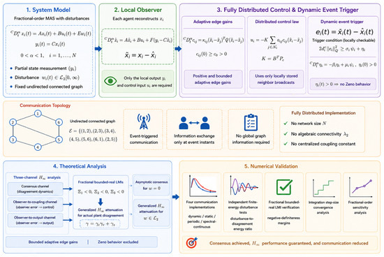
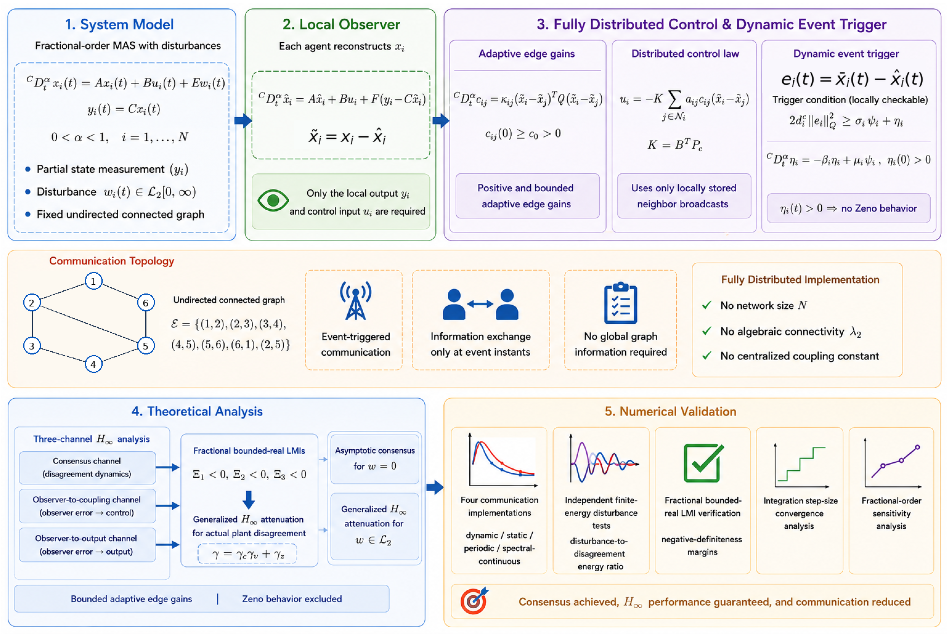
The overall methodological framework is illustrated in Figure 1. It integrates the fractional-order agent model, local observer, adaptive edge coupling, distributed controller, dynamic event trigger, three-channel performance analysis, and numerical validation.

Figure 1. Overall methodological framework of the proposed fully distributed dynamic event-triggered observer-based $H_{\infty }$ consensus method.

Table 1 summarizes the methodological differences between the proposed approach and representative related designs.

Table 1. Methodological comparison with representative related designs.

Method	Partial-State Measurement	No Graph Spectrum in Implementation	Dynamic Event Trigger	Disturbance Attenuation
Li et al. [23]	Yes	No	No	$H_{\infty }$
Cheng and Li [17]	No	Yes	Static	Not considered
Xia et al. [20]	No	Yes	Yes	Not considered
Proposed method	Yes	Yes	Yes	Generalized $H_{\infty }$

The remainder of this paper is organized as follows. Section 2 presents the problem formulation and performance definition. Section 3 introduces the observer, adaptive controller, and triggering mechanism. Section 4 establishes the stability, attenuation, and Zeno-exclusion results. Section 5 reports the numerical simulations, and Section 6 concludes the paper.

2. Preliminaries and Problem Formulation

2.1. Graph Notation

Let $\mathcal{G}=(\mathcal{V},\mathcal{E},\mathcal{A})$ be a fixed undirected graph with node set $\mathcal{V}=\{1,\dots ,N\}$, edge set $\mathcal{E}$, and adjacency matrix $\mathcal{A}=\left[a_{ij}\right]$. The neighbor set of node i is ${\mathcal{N}}_i=\{j:(i,j)\in \mathcal{E}\}$. The graph Laplacian is $L=D-\mathcal{A}$, where $D=\mathrm{diag}(d_1,\dots ,d_N)$ and $d_i={\sum }_j{a}_{ij}$. Let $H\in {\mathbb{R}}^{N\times M}$ be an arbitrarily oriented incidence matrix, where $M=\left|\mathcal{E}\right|$, so that $L=H{H}^T$. Define

$${\mathcal{M}}_N=I_N-{\displaystyle \frac{1}{N}}{\mathbf{1}}_N{\mathbf{1}}_N^T.$$

(1)

For a stacked vector $x=\mathrm{col}(x_1,\dots ,x_N)$, $({\mathcal{M}}_N\otimes I)x$ is its disagreement component.

Assumption 1.

The graph $\mathcal{G}$ is connected.

Remark 1.

Assumption 1 is the minimum structural requirement for agreement over a fixed undirected network: without connectivity, different connected components cannot exchange information and global consensus is impossible. The fixed undirected setting allows the analysis to focus on the fractional-memory, output-feedback, adaptive-coupling, and event-triggering mechanisms. Importantly, no agent is assumed to know L, ${\lambda }_2\left(L\right)$, or the network size. Directed and switching graphs require additional left-eigenvector or joint-connectivity arguments and are outside the present theorem.

2.2. Fractional Calculus and Bounded-Real Inequalities

For $0<\alpha <1$, the Caputo derivative of an absolutely continuous signal $x\left(t\right)$ is

$${{}^{C}D}_t^{\alpha }x\left(t\right)={\displaystyle \frac{1}{\mathsf{\Gamma }(1-\alpha )}}{\int }_0^t{(t-s)}^{-\alpha }\dot{x}\left(s\right)ds.$$

(2)

The corresponding fractional integral is

$$I_t^{\alpha }f\left(t\right)={\displaystyle \frac{1}{\mathsf{\Gamma }\left(\alpha \right)}}{\int }_0^t{(t-s)}^{\alpha -1}f\left(s\right)ds.$$

(3)

Lemma 1

(Fractional quadratic inequality [23]). For $P=P^T\succ 0$ and a differentiable vector $x\left(t\right)$,

$${\displaystyle \frac{1}{2}}{{}^{C}D}_t^{\alpha }\left(x^{T}Px\right)\le x^{T}P{{}^{C}D}_t^{\alpha }x.$$

(4)

Lemma 2

(Hölder continuity of a Caputo trajectory [2]). If $x\left(t\right)=x\left(0\right)+I_t^{\alpha }f\left(t\right)$ and $∥f\left(t\right)∥\le M_T$ on $[0,T]$, then for all $0\le s<t\le T$,

$$∥x\left(t\right)-x\left(s\right)∥\le {\displaystyle \frac{2M_T}{\mathsf{\Gamma }(\alpha +1)}}{(t-s)}^{\alpha }.$$

(5)

Let $\vartheta =\alpha \pi /2$ and define

$$\begin{array}{cc}\hfill {\mathcal{S}}_{\alpha }(P,X)& =\left[\begin{array}{cc}\sin \vartheta \mathrm{He}\left(PX\right)& \cos \vartheta (X^{T}P-PX)\\ \ast & \sin \vartheta \mathrm{He}\left(PX\right)\end{array}\right],\hfill \end{array}$$

(6)

$$\begin{array}{cc}\hfill {\mathcal{E}}_{\alpha }(P,G)& =\left[\begin{array}{cc}\sin \vartheta PG& \cos \vartheta PG\\ -\cos \vartheta PG& \sin \vartheta PG\end{array}\right].\hfill \end{array}$$

(7)

Lemma 3

(Fractional bounded-real condition [24]). Consider ${{}^{C}D}_t^{\alpha }x=Xx+Gw$ and $z=C_{o}x$. If $P=P^T\succ 0$ and $\gamma >0$ satisfy

$$\mathcal{B}(P,X,G,C_o,\gamma )=\left[\begin{array}{cc}{\mathcal{S}}_{\alpha }(P,X)+I_2\otimes C_o^T{C}_o& {\mathcal{E}}_{\alpha }(P,G)\\ \ast & -{\gamma }^{2}I\end{array}\right]\prec 0,$$

(8)

then X is α-stable and the input-output channel has an $H_{\infty }$ gain smaller than γ under the standard zero-initial-state interpretation. Nonzero initial states add a finite storage term.

2.3. Agent Dynamics and Performance Objective

Consider N identical agents

$$\begin{array}{cc}\hfill {{}^{C}D}_t^{\alpha }{x}_i& =A{x}_i+B{u}_i+E{w}_i,\hfill \end{array}$$

(9)

$$\begin{array}{cc}\hfill y_i& =C{x}_i,z_i=C_z{x}_i,\hfill \end{array}$$

(10)

where $x_i\in {\mathbb{R}}^n$, $u_i\in {\mathbb{R}}^m$, $y_i\in {\mathbb{R}}^p$, $w_i\in {\mathbb{R}}^q$, and $z_i\in {\mathbb{R}}^r$. Only $y_i$ is measured. Each disturbance is assumed piecewise continuous and locally essentially bounded, and the stacked disturbance satisfies $w=\mathrm{col}(w_1,\dots ,w_N)\in {\mathcal{L}}_2[0,\infty )\cap {\mathcal{L}}_{\infty ,\mathrm{loc}}[0,\infty )$. Define

$$z_c=({\mathcal{M}}_N\otimes C_z)x.$$

(11)

Assumption 2.

The pair $(A,B)$ is stabilizable, $(A,C)$ is detectable, and E and $C_z$ are known.

Remark 2.

The stabilizability and detectability requirements are standard for output-feedback consensus: they guarantee that the controllable disagreement modes can be damped and that the unavailable state can be reconstructed from $y_i$. Knowledge of E and $C_z$ is needed only to formulate and verify the local disturbance-attenuation inequalities. The condition $w\in {\mathcal{L}}_2$ is the finite-energy signal class underlying the $H_{\infty }$ statement, whereas local essential boundedness and piecewise continuity are invoked only in the Zeno-exclusion argument to ensure a bounded observer right-hand side, and hence Hölder continuity, on every finite interval. The theorem does not claim rejection of arbitrary non-decaying or infinite-energy disturbances.

Definition 1.

The closed-loop system achieves generalized observer-based $H_{\infty }$ consensus with level γ if: (i) $x_i\left(t\right)-x_j\left(t\right)\to 0$ for all $i,j$ when $w\equiv 0$; and (ii), for every $T>0$,

$${∥z_c∥}_{2,[0,T]}\le \gamma {∥w∥}_{2,[0,T]}+\sqrt{{\mathcal{V}}_0},$$

(12)

where ${\mathcal{V}}_0$ depends only on initial plant, observer, adaptive-gain, and triggering states. The term ${\mathcal{V}}_0$ is necessary because the fully distributed adaptive controller contains nonzero internal storage.

Remark 3.

Definition 1 distinguishes the proved dissipative bound from an empirical finite-horizon energy ratio. In Section 5, consensus tests use nonzero disagreement and are therefore reported with their initial-storage contribution, whereas separate zero-physical-initial-state tests are used to evaluate disturbance attenuation.

3. Fully Distributed Dynamic Event-Triggered Design

As illustrated in Figure 1, the proposed distributed design consists of a local state observer, fractional adaptive edge couplings, an observer-based distributed controller, and a locally evaluated dynamic event-triggered communication mechanism.

3.1. Local Observer

For each agent, construct

$${{}^{C}D}_t^{\alpha }{\widehat{x}}_i=A{\widehat{x}}_i+B{u}_i+F(y_i-C{\widehat{x}}_i).$$

(13)

The observation error ${\tilde{x}}_i=x_i-{\widehat{x}}_i$ satisfies

$${{}^{C}D}_t^{\alpha }{\tilde{x}}_i=(A-FC){\tilde{x}}_i+E{w}_i.$$

(14)

Thus, observer-error dynamics are independent of the graph and control input.

3.2. Broadcast Variables and Fractional Adaptive Coupling

Let $t_k^i$ denote the kth transmission instant of agent i. Define

$${\overline{x}}_i\left(t\right)={\widehat{x}}_i\left(t_k^i\right),e_i\left(t\right)={\overline{x}}_i\left(t\right)-{\widehat{x}}_i\left(t\right),t\in [t_k^i,t_{k+1}^i).$$

(15)

For every edge $(i,j)\in \mathcal{E}$, assign $c_{ij}=c_{ji}$ and update it by

$${{}^{C}D}_t^{\alpha }{c}_{ij}={\kappa }_{ij}{({\overline{x}}_i-{\overline{x}}_j)}^{T}Q({\overline{x}}_i-{\overline{x}}_j),c_{ij}\left(0\right)\ge c_0>0,$$

(16)

where ${\kappa }_{ij}>0$. Select

$$K=B^T{P}_c,Q=P_{c}B{B}^T{P}_c,$$

(17)

and apply

$$u_i=-K\sum _{j\in {\mathcal{N}}_i}{a}_{ij}{c}_{ij}({\overline{x}}_i-{\overline{x}}_j).$$

(18)

Every quantity in (16)–(18) is locally available. Although ${{}^{C}D}_t^{\alpha }{c}_{ij}\ge 0$, $c_{ij}\left(t\right)$ need not be monotone in the ordinary integer-order sense. The integral representation nevertheless gives $c_{ij}\left(t\right)=c_{ij}\left(0\right)+I_t^{\alpha }\left({\kappa }_{ij}{∥{\overline{x}}_i-{\overline{x}}_j∥}_Q^2\right)\ge c_0$.

Remark 4.

The distinction from a fixed spectral coupling is fundamental for implementation. A conventional fixed-gain design selects a common gain from a condition involving the smallest nonzero Laplacian eigenvalue, so a topology change generally requires recomputing that gain. Here each $c_{ij}$ is updated only from the latest broadcasts of the two incident agents. The proof introduces a sufficiently large constant $c^{★}$ only to certify the existence of adequate aggregate damping; $c^{★}$ and ${\lambda }_2\left(L\right)$ never enter the implemented observer, controller, adaptive law, or trigger. Positivity of $c_{ij}$ follows from its fractional integral representation, whereas boundedness follows from the closed-loop storage argument; ordinary monotonicity is neither required nor claimed.

3.3. Explicit Weighted Dynamic Event Trigger

Define the local weighted degree and stored edge energy

$$\begin{array}{cc}\hfill d_i^c\left(t\right)& =\sum _{j\in {\mathcal{N}}_i}{a}_{ij}{c}_{ij}\left(t\right),\hfill \end{array}$$

(19)

$$\begin{array}{cc}\hfill {\psi }_i\left(t\right)& =\sum _{j\in {\mathcal{N}}_i}{a}_{ij}{∥{\overline{x}}_i-{\overline{x}}_j∥}_Q^2.\hfill \end{array}$$

(20)

Each node maintains

$${{}^{C}D}_t^{\alpha }{\eta }_i=-{\beta }_i{\eta }_i+{\mu }_i{\psi }_i,{\eta }_i\left(0\right)>0,$$

(21)

where ${\beta }_i>0$ and ${\mu }_i\ge 0$. The next event time is

$$t_{k+1}^i=\inf \left\{t>t_k^i:2d_i^c{∥e_i∥}_Q^2\ge {\sigma }_i{\psi }_i+{\eta }_i\right\},$$

(22)

where ${\sigma }_i\ge 0$. Between two consecutive events,

$$2d_i^c{∥e_i∥}_Q^2<{\sigma }_i{\psi }_i+{\eta }_i.$$

(23)

Unlike a graph-wide small-gain assumption, (23) is enforced directly by the local trigger and can therefore be used without an offline global verification step.

Remark 5.

The weighted degree $d_i^c$ is not an additional global variable. Agent i obtains it by summing only its incident adaptive gains. This weighting makes the trigger scale with the same couplings that multiply the broadcast error in the closed-loop dynamics, so the local inequality (23) directly bounds the network error term used in the stability proof. In contrast, an unweighted threshold would generally require a separate global upper bound on the adaptive couplings or the graph degree.

3.4. Design Procedure and Parameter Selection

The design can be implemented in the following order. First, choose an observer gain F such that $A-FC$ is $\alpha$-stable and determine $P_v,P_z\succ 0$ and channel levels ${\gamma }_v,{\gamma }_z$ satisfying (25) and (26). Second, determine $P_c\succ 0$ such that (24) is feasible and then set $K=B^T{P}_c$ and $Q=P_{c}B{B}^T{P}_c$; this structural choice is essential for Proposition 1. Third, select the local adaptive parameters $c_0>0$ and ${\kappa }_{ij}>0$. Finally, select ${\sigma }_i\ge 0$, ${\beta }_i>0$, ${\mu }_i\ge 0$, and ${\eta }_i\left(0\right)>0$ to trade communication frequency against the stored trigger margin. These trigger parameters are local tuning variables and do not require N, ${\lambda }_2\left(L\right)$, or any centralized coupling constant. For the reported benchmark, $F={[1,1]}^T$ is fixed first, and the candidate matrices $P_c$, $P_v$, and $P_z$ together with the channel levels are retained only when the maximum eigenvalues of ${\mathcal{B}}_c$, ${\mathcal{B}}_v$, and ${\mathcal{B}}_z$ are strictly negative. With F, $P_c$, $P_v$, $P_z$, and K fixed, the adaptive and triggering parameters are tuned subsequently, thereby separating certificate verification from communication tuning. The resulting fully distributed implementation procedure at each agent is summarized in Algorithm 1.

Algorithm 1 Local implementation at agent i.

1: Initialize ${\widehat{x}}_i\left(0\right)$, ${\overline{x}}_i\left(0\right)={\widehat{x}}_i\left(0\right)$, ${\eta }_i\left(0\right)>0$, and incident $c_{ij}\left(0\right)\ge c_0$. 2: while the system operates do 3:    Update the observer by (13) using $y_i$ and $u_i$. 4:    Update each incident adaptive gain by (16) and ${\eta }_i$ by (21). 5:    Compute $d_i^c$, ${\psi }_i$, and $u_i$ from locally stored neighbor broadcasts. 6:    if condition (22) is satisfied then 7:       Broadcast ${\widehat{x}}_i\left(t\right)$ and set ${\overline{x}}_i\leftarrow {\widehat{x}}_i\left(t\right)$. 8:    end if 9: end while

4. Stability and Disturbance-Attenuation Analysis

Define $X_c=A-BK$ and $X_o=A-FC$. The synthesis uses the following three local inequalities:

$$\begin{array}{cc}\hfill {\mathcal{B}}_c& =\mathcal{B}(P_c,X_c,I_n,C_z,{\gamma }_c)\prec 0,\hfill \end{array}$$

(24)

$$\begin{array}{cc}\hfill {\mathcal{B}}_v& =\mathcal{B}(P_v,X_o,E,FC,{\gamma }_v)\prec 0,\hfill \end{array}$$

(25)

$$\begin{array}{cc}\hfill {\mathcal{B}}_z& =\mathcal{B}(P_z,X_o,E,C_z,{\gamma }_z)\prec 0.\hfill \end{array}$$

(26)

The first channel maps the observer-induced coupling input to the estimated-state disagreement output. The second and third channels map the physical disturbance to $FC{\tilde{x}}_i$ and $C_z{\tilde{x}}_i$, respectively.

Remark 6.

The multiplication-plus-addition form of the final attenuation bound follows from the signal interconnection rather than from an arbitrary combination of three gains. The disturbance first passes through the observer-to-coupling map with gain ${\gamma }_v$ and then through the consensus map with gain ${\gamma }_c$, producing the cascade contribution ${\gamma }_c{\gamma }_v$. The actual plant output also contains the direct observer-output term with gain ${\gamma }_z$. Since $z_c$ is the sum of these two contributions, the triangle inequality yields ${\gamma }_c{\gamma }_v+{\gamma }_z$.

Proposition 1.

Let $K=B^T{P}_c$. If (24) holds, then the same bounded-real inequality remains feasible when $X_c$ is replaced by $A-\lambda BK$ for any $\lambda \ge 1$.

Proof. 

Because $P_{c}BK=P_{c}B{B}^T{P}_c=Q=Q^T⪰0$,

$${\mathcal{S}}_{\alpha }(P_c,A-\lambda BK)={\mathcal{S}}_{\alpha }(P_c,A-BK)-2(\lambda -1)\sin \vartheta \mathrm{diag}(Q,Q).$$

(27)

The additional term is negative semidefinite, while the input and output blocks of (24) are unchanged. Hence feasibility at $\lambda =1$ implies feasibility for all $\lambda \ge 1$. □

Theorem 1.

Suppose Assumptions 1 and 2 hold. Assume that matrices $P_c,P_v,P_z\succ 0$, F, and positive scalars ${\gamma }_c,{\gamma }_v,{\gamma }_z$ satisfy (17) and (24)–(26). Let the disturbance be piecewise continuous with $w\in {\mathcal{L}}_2[0,\infty )\cap {\mathcal{L}}_{\infty ,\mathrm{loc}}[0,\infty )$. For arbitrary local parameters $c_0>0$, ${\kappa }_{ij}>0$, ${\sigma }_i\ge 0$, ${\beta }_i>0$, ${\mu }_i\ge 0$, and ${\eta }_i\left(0\right)>0$, apply (13), (16), (18), (21), and (22). Then:

1. 

all observation errors, disagreement signals, adaptive gains, and internal triggering variables remain bounded for finite-energy disturbances;

2. 

when $w\equiv 0$, ${\tilde{x}}_i\left(t\right)\to 0$ and $x_i\left(t\right)-x_j\left(t\right)\to 0$ for all $i,j$;

3. 

the generalized attenuation level in Definition 1 can be chosen as

$$\gamma ={\gamma }_c{\gamma }_v+{\gamma }_z;$$

(28)

4. 

the event sequence of every agent has no finite accumulation point; therefore, Zeno behavior is excluded.

Proof. 

Let $\widehat{x}=\mathrm{col}({\widehat{x}}_1,\dots ,{\widehat{x}}_N)$, $e=\mathrm{col}(e_1,\dots ,e_N)$, and

$$\xi =({\mathcal{M}}_N\otimes I_n)\widehat{x}.$$

(29)

For edge ℓ, let $h_{\ell }$ be the corresponding incidence column and define

$$q_{\ell }=(h_{\ell }^T\otimes I_n)\xi ,r_{\ell }=(h_{\ell }^T\otimes I_n)e,{\overline{q}}_{\ell }=q_{\ell }+r_{\ell }.$$

(30)

Let $C_e=\mathrm{diag}(c_1,\dots ,c_M)$ and $\overline{x}=\mathrm{col}({\overline{x}}_1,\dots ,{\overline{x}}_N)$. Stacking (13) gives

$${{}^{C}D}_t^{\alpha }\widehat{x}=(I_N\otimes A)\widehat{x}+(I_N\otimes B)u+(I_N\otimes FC)\tilde{x}.$$

(31)

For an arbitrarily oriented incidence matrix, the distributed controller (18) can be written as

$$u=-(H{C}_e{H}^T\otimes K)\overline{x}.$$

(32)

Because ${\mathcal{M}}_{N}H=H$, $H^T{\mathbf{1}}_N=0$, and $\overline{x}=\widehat{x}+e$, one has

$$(H^T\otimes I_n)\overline{x}=(H^T\otimes I_n)(\xi +e)=\overline{q}.$$

(33)

Premultiplying (31) by ${\mathcal{M}}_N\otimes I_n$, substituting (32) and (33), and using $\xi =({\mathcal{M}}_N\otimes I_n)\widehat{x}$ therefore yields

$${{}^{C}D}_t^{\alpha }\xi =(I_N\otimes A)\xi -(H{C}_e\otimes BK)\overline{q}+({\mathcal{M}}_N\otimes FC)\tilde{x},$$

(34)

where $\overline{q}=\mathrm{col}({\overline{q}}_1,\dots ,{\overline{q}}_M)$ and $\tilde{x}=\mathrm{col}({\tilde{x}}_1,\dots ,{\tilde{x}}_N)$.

For analysis only, choose $c^{★}>0$ and consider

$$V_c={\xi }^T(I_N\otimes P_c)\xi +{\displaystyle \sum _{\ell =1}^M}{\displaystyle \frac{{(c_{\ell }-c^{★})}^2}{2{\kappa }_{\ell }}}+\varpi c^{★}{\displaystyle \sum _{i=1}^N}{\eta }_i,$$

(35)

where $\varpi >0$ is a proof-only weighting scalar that will be specified explicitly below. By Lemma 1, (16), and $Q=P_{c}BK$, the controller and adaptive-gain terms satisfy

$$\begin{array}{cc}\hfill {\mathcal{T}}_{ca}& =-2{\displaystyle \sum _{\ell =1}^M}{c}_{\ell }{q}_{\ell }^{T}Q{\overline{q}}_{\ell }+{\displaystyle \sum _{\ell =1}^M}(c_{\ell }-c^{★}){\overline{q}}_{\ell }^{T}Q{\overline{q}}_{\ell }\hfill \\ \hfill & =-{\displaystyle \sum _{\ell =1}^M}(c_{\ell }+c^{★}){∥{\overline{q}}_{\ell }∥}_Q^2+2{\displaystyle \sum _{\ell =1}^M}{c}_{\ell }{r}_{\ell }^{T}Q{\overline{q}}_{\ell }\hfill \\ \hfill & \le -c^{★}{\displaystyle \sum _{\ell =1}^M}{∥{\overline{q}}_{\ell }∥}_Q^2+{\displaystyle \sum _{\ell =1}^M}{c}_{\ell }{∥r_{\ell }∥}_Q^2.\hfill \end{array}$$

(36)

The last step follows from $2r^{T}Q\overline{q}\le r^{T}Qr+{\overline{q}}^{T}Q\overline{q}$.

The event-error term is bounded directly by the trigger. Indeed,

$$\begin{array}{cc}\hfill \sum _{\ell =(i,j)}{c}_{ij}{∥e_i-e_j∥}_Q^2& \le 2{\displaystyle \sum _{i=1}^N}{d}_i^c{∥e_i∥}_Q^2\hfill \\ \hfill & \le {\displaystyle \sum _{i=1}^N}{\sigma }_i{\psi }_i+{\displaystyle \sum _{i=1}^N}{\eta }_i\hfill \\ \hfill & \le 2\overline{\sigma }{\displaystyle \sum _{\ell =1}^M}{∥{\overline{q}}_{\ell }∥}_Q^2+{\displaystyle \sum _{i=1}^N}{\eta }_i,\hfill \end{array}$$

(37)

where $\overline{\sigma }={\max }_i{\sigma }_i$. Combining (36) and (37), and the fractional derivative of the last term in (35) gives

$${\mathcal{T}}_{ca\eta }\le -g\left(c^{★}\right){\displaystyle \sum _{\ell =1}^M}{∥{\overline{q}}_{\ell }∥}_Q^2-h\left(c^{★}\right){\displaystyle \sum _{i=1}^N}{\eta }_i,$$

(38)

where

$$g\left(c^{★}\right)=c^{★}(1-2\varpi \overline{\mu })-2\overline{\sigma },h\left(c^{★}\right)=\varpi c^{★}\underline{\beta }-1,$$

(39)

with $\overline{\mu }={\max }_i{\mu }_i$ and $\underline{\beta }={\min }_i{\beta }_i$.

Because $c_{\ell }\left(t\right)\ge c_0$, for any $\nu >0$,

$$\begin{array}{cc}\hfill {\displaystyle \sum _{\ell =1}^M}{∥q_{\ell }∥}_Q^2& \le (1+\nu ){\displaystyle \sum _{\ell =1}^M}{∥{\overline{q}}_{\ell }∥}_Q^2+(1+{\nu }^{-1}){\displaystyle \sum _{\ell =1}^M}{∥r_{\ell }∥}_Q^2\hfill \\ \hfill & \le a_{\nu }{\displaystyle \sum _{\ell =1}^M}{∥{\overline{q}}_{\ell }∥}_Q^2+b_{\nu }{\displaystyle \sum _{i=1}^N}{\eta }_i,\hfill \end{array}$$

(40)

where

$$a_{\nu }=1+\nu +{\displaystyle \frac{2\overline{\sigma }(1+{\nu }^{-1})}{c_0}},b_{\nu }={\displaystyle \frac{1+{\nu }^{-1}}{c_0}}.$$

(41)

Define

$${\varpi }_{\min }={\displaystyle \frac{b_{\nu }}{a_{\nu }\underline{\beta }+2\overline{\mu }{b}_{\nu }}}.$$

(42)

If $\overline{\mu }>0$, choose explicitly

$$\varpi ={\displaystyle \frac{1}{2}}\left({\varpi }_{\min }+{\displaystyle \frac{1}{2\overline{\mu }}}\right),$$

(43)

whereas for $\overline{\mu }=0$ one may take $\varpi ={\varpi }_{\min }+1$. Since $\underline{\beta }>0$, ${\varpi }_{\min }<1/\left(2\overline{\mu }\right)$ whenever $\overline{\mu }>0$, so the stated midpoint is well defined and satisfies the required inequalities. Consequently, a sufficiently large proof constant $c^{★}$ can be chosen such that

$${\displaystyle \frac{g\left(c^{★}\right){\lambda }_2\left(L\right)}{a_{\nu }}}\ge 2,{\displaystyle \frac{g\left(c^{★}\right)b_{\nu }}{a_{\nu }}}-h\left(c^{★}\right)<0.$$

(44)

This constant is not used by any agent. Using ${\sum }_{\ell }{∥q_{\ell }∥}_Q^2={\xi }^T(L\otimes Q)\xi \ge {\lambda }_2\left(L\right){\xi }^T(I_N\otimes Q)\xi$, inequalities (38)–(44) imply

$${\mathcal{T}}_{ca\eta }\le -2{\xi }^T(I_N\otimes Q)\xi -{\delta }_{\eta }{\displaystyle \sum _{i=1}^N}{\eta }_i$$

(45)

for some ${\delta }_{\eta }>0$. Thus, the adaptive network supplies at least the damping associated with the local matrix $A-BK$. Inequality (45) is therefore not used as a separate $H_{\infty }$ certificate; rather, it establishes that the actual network dissipation is no weaker than the nominal consensus channel certified by $A-BK$. Proposition 1 then guarantees that any larger effective coupling contributes only an additional negative-semidefinite term and cannot destroy feasibility of ${\mathcal{B}}_c\prec 0$.

Let $v=({\mathcal{M}}_N\otimes FC)\tilde{x}$ and $z_{\xi }=(I_N\otimes C_z)\xi$. Applying Lemma 3 to the nominal consensus channel (24), with the adaptive-network damping justified above, gives

$${∥z_{\xi }∥}_{2,[0,T]}\le {\gamma }_c{∥v∥}_{2,[0,T]}+\sqrt{V_{c0}}.$$

(46)

The observer Equation (14) and inequalities (25) and (26) yield

$$\begin{array}{cc}\hfill {∥(I_N\otimes FC)\tilde{x}∥}_{2,[0,T]}& \le {\gamma }_v{∥w∥}_{2,[0,T]}+\sqrt{V_{v0}},\hfill \end{array}$$

(47)

$$\begin{array}{cc}\hfill {∥(I_N\otimes C_z)\tilde{x}∥}_{2,[0,T]}& \le {\gamma }_z{∥w∥}_{2,[0,T]}+\sqrt{V_{z0}}.\hfill \end{array}$$

(48)

Since ${∥{\mathcal{M}}_N∥}_2=1$ and

$$z_c=(I_N\otimes C_z)\xi +({\mathcal{M}}_N\otimes C_z)\tilde{x},$$

(49)

combining (46)–(48) gives (12) with $\gamma ={\gamma }_c{\gamma }_v+{\gamma }_z$ and a finite initial-storage term ${\mathcal{V}}_0$.

When $w\equiv 0$, the strict LMIs and (45) imply boundedness and decay of $\xi$ and $\tilde{x}$. A fractional LaSalle argument then gives $\xi \to 0$ and $\tilde{x}\to 0$, which implies $x_i-x_j\to 0$. Boundedness of the shifted-gain terms in (35) gives bounded adaptive gains.

It remains to exclude Zeno behavior. The solution of (21) is

$$\begin{array}{cc}\hfill {\eta }_i\left(t\right)=& {\eta }_i\left(0\right)E_{\alpha }(-{\beta }_i{t}^{\alpha })\hfill \\ \hfill & +{\mu }_i{\int }_0^t{(t-s)}^{\alpha -1}{E}_{\alpha ,\alpha }[-{\beta }_i{(t-s)}^{\alpha }]{\psi }_i\left(s\right)ds,\hfill \end{array}$$

(50)

which is positive for $0<\alpha <1$. On any finite interval $[0,T]$, the stated local boundedness of w, together with bounded closed-loop states and inputs, implies finite constants ${\underline{\eta }}_T>0$, ${\overline{d}}_T<\infty$, and $M_T<\infty$ such that ${\eta }_i\ge {\underline{\eta }}_T$, $d_i^c\le {\overline{d}}_T$, and the observer right-hand side is bounded by $M_T$. Lemma 2 then gives

$$∥e_i\left(t\right)∥\le {\displaystyle \frac{2M_T}{\mathsf{\Gamma }(\alpha +1)}}{(t-t_k^i)}^{\alpha }.$$

(51)

Starting from $e_i\left(t_k^i\right)=0$, condition (22) cannot be reached before

$$t-t_k^i\ge {\left[{\displaystyle \frac{\mathsf{\Gamma }(\alpha +1)}{2M_T}}\sqrt{{\displaystyle \frac{{\underline{\eta }}_T}{2{\overline{d}}_T{\lambda }_{\max }\left(Q\right)}}}\right]}^{1/\alpha }>0.$$

(52)

Hence, no infinite number of events can occur in a finite interval. □

Remark 7.

The lower inter-event-time estimate in (52) is established on an arbitrary finite interval $[0,T]$. Its constants may depend on T, so the theorem does not claim a single globally uniform dwell time valid on $[0,\infty )$. What is proved is the property required to exclude Zeno behavior: every finite interval admits a strictly positive event-separation bound and therefore cannot contain infinitely many triggering instants.

Remark 8.

The adjective “fully distributed” concerns implementation. The proof uses ${\lambda }_2\left(L\right)$ only to establish the existence of $c^{★}$ in (44); neither $c^{★}$ nor ${\lambda }_2\left(L\right)$ appears in the observer, controller, adaptive law, or trigger.

5. Numerical Simulations

5.1. System and Graph

Consider six fractional-order double-integrator agents with $\alpha =0.92$ and

$$A=\left[\begin{array}{cc}0& 1\\ 0& 0\end{array}\right],B=\left[\begin{array}{c}0\\ 1\end{array}\right],C=\left[\begin{array}{cc}1& 0\end{array}\right],E=\left[\begin{array}{c}0\\ 1\end{array}\right],C_z=\mathrm{diag}(1,\sqrt{0.2}).$$

(53)

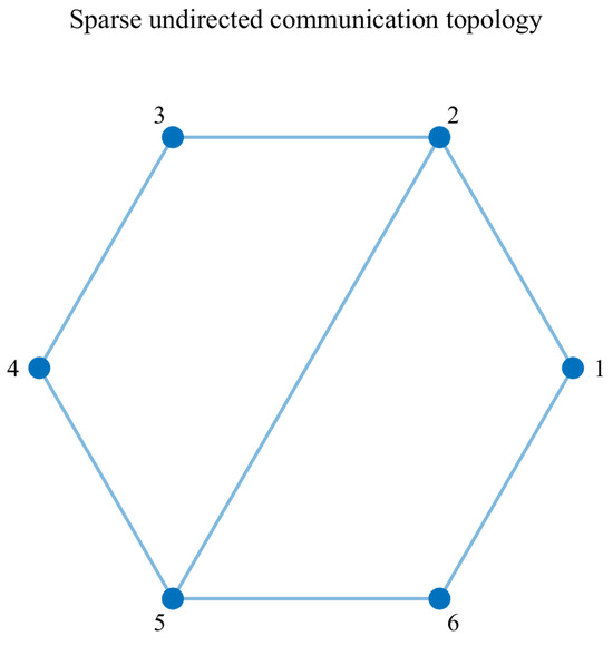
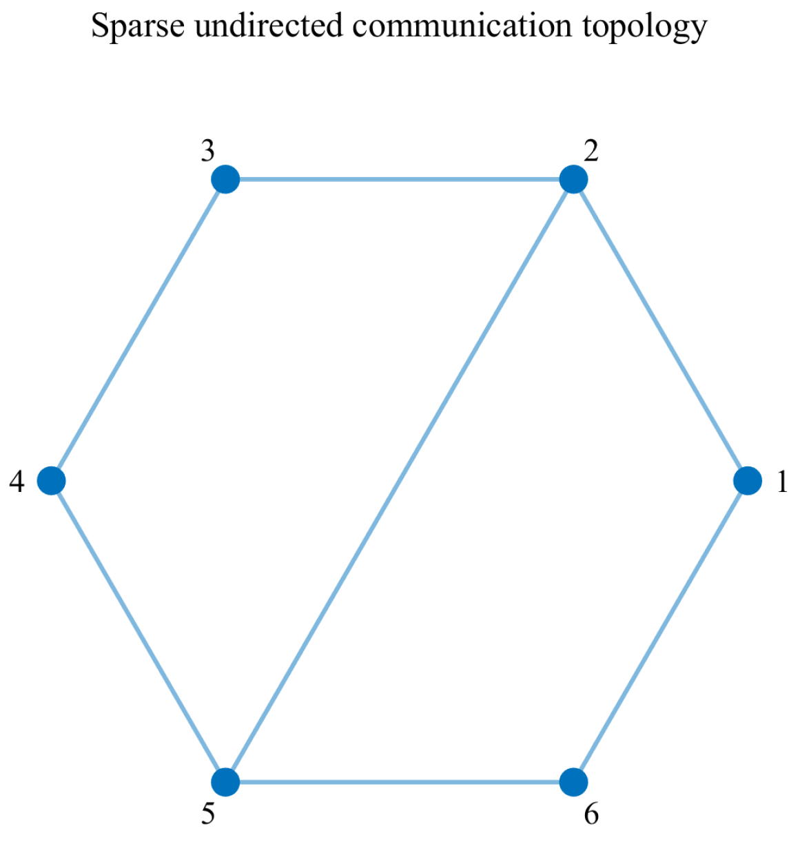
The double-integrator model is selected so that consensus convergence cannot be attributed to the autonomous asymptotic stability of the isolated agents. The edge set is

$$\mathcal{E}=\left\{\right(1,2),(2,3),(3,4),(4,5),(5,6),(6,1),(2,5\left)\right\},$$

(54)

which gives the sparse connected graph in Figure 2.

Figure 2. Sparse undirected communication topology used in the simulations.

The selected matrices and gains are

$$\begin{array}{cccccc}\hfill P_c& =\left[\begin{array}{cc}4.55& 3.75\\ 3.75& 4.00\end{array}\right],\hfill & \hfill K& =\left[\begin{array}{cc}3.75& 4.00\end{array}\right],\hfill & \hfill F& =\left[\begin{array}{c}1\\ 1\end{array}\right],\hfill \end{array}$$

(55)

$$\begin{array}{cccc}\hfill P_v& =\left[\begin{array}{cc}3.0078& -1.5039\\ -1.5039& 4.5117\end{array}\right],\hfill & \hfill P_z& =\left[\begin{array}{cc}1.5689& -0.7844\\ -0.7844& 2.3533\end{array}\right].\hfill \end{array}$$

(56)

The channel levels are ${\gamma }_c=1.4$, ${\gamma }_v=3.7$, and ${\gamma }_z=2.8$, giving $\gamma =7.98$. The numerical maximum eigenvalues of the three LMI matrices are listed in Table 2; all are strictly negative.

Table 2. Numerical verification of the local fractional bounded-real inequalities.

Channel	Selected Level	Maximum LMI Eigenvalue
Consensus channel, (24)	${\gamma }_c=1.4$	$-0.05087$
Observer-to-coupling channel, (25)	${\gamma }_v=3.7$	$-0.18260$
Observer-to-output channel, (26)	${\gamma }_z=2.8$	$-0.09227$

The adaptive and trigger parameters are $c_{ij}\left(0\right)=0.60$, ${\kappa }_{ij}=0.015$, ${\sigma }_i=0.040$, ${\eta }_i\left(0\right)=0.080$, ${\beta }_i=0.350$, and ${\mu }_i=0.015$. The initial plant states are

$$\begin{array}{cccccc}\hfill x_1\left(0\right)& ={[1.8,-0.4]}^T,\hfill & \hfill x_2\left(0\right)& ={[-1.2,0.8]}^T,\hfill & \hfill x_3\left(0\right)& ={[0.7,-0.6]}^T,\hfill \end{array}$$

(57)

$$\begin{array}{cccccc}\hfill x_4\left(0\right)& ={[-1.8,0.3]}^T,\hfill & \hfill x_5\left(0\right)& ={[1.2,-0.9]}^T,\hfill & \hfill x_6\left(0\right)& ={[-0.3,0.5]}^T.\hfill \end{array}$$

(58)

The observer states are initialized at $0.5x_i\left(0\right)$ plus fixed deterministic perturbations. The disturbance is a finite-support combination of exponentially decaying sinusoids and smooth pulses. The simulation horizon is 20 s and the nominal step is $h=0.02$ s.

5.2. Fractional Numerical Implementation

The Caputo equation ${{}^{C}D}_t^{\alpha }X=f(t,X)$ is integrated by the product-rectangle approximation

$$X\left(t_n\right)=X\left(0\right)+{\displaystyle \frac{h^{\alpha }}{\mathsf{\Gamma }(\alpha +1)}}{\displaystyle \sum _{j=0}^{n-1}}\left[{(n-j)}^{\alpha }-{(n-j-1)}^{\alpha }\right]f(t_j,X\left(t_j\right)).$$

(59)

This explicit memory formula is closely related to standard predictor–corrector discretizations for Caputo equations [27]. Plant, observer, adaptive-gain, and dynamic-trigger variables use the same fractional order. Events are detected on the integration grid.

5.3. Consensus and Observer Responses

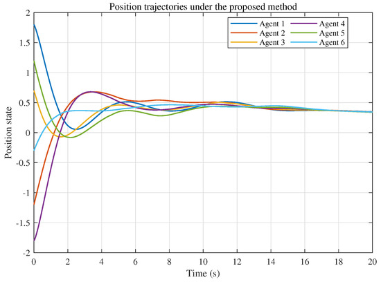
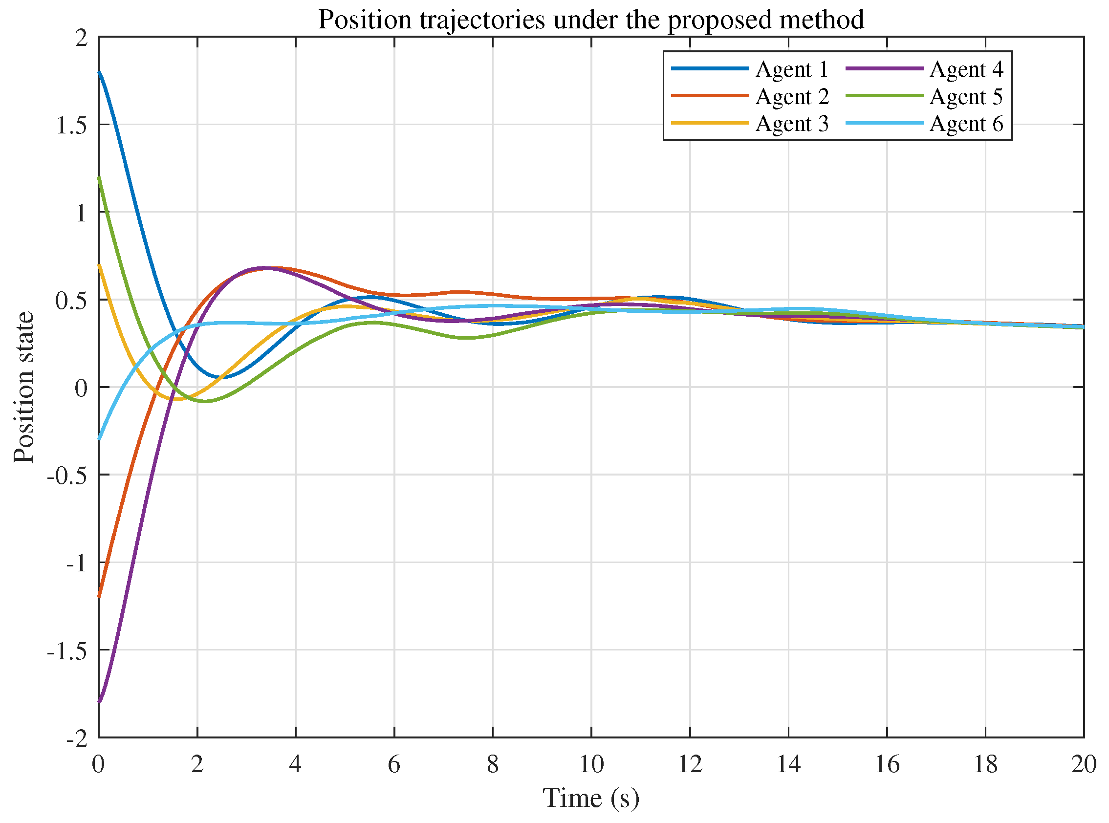
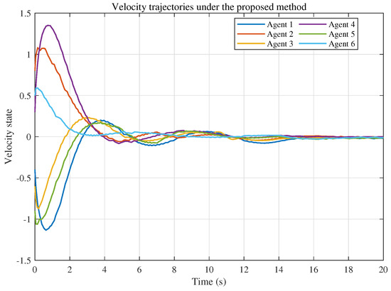
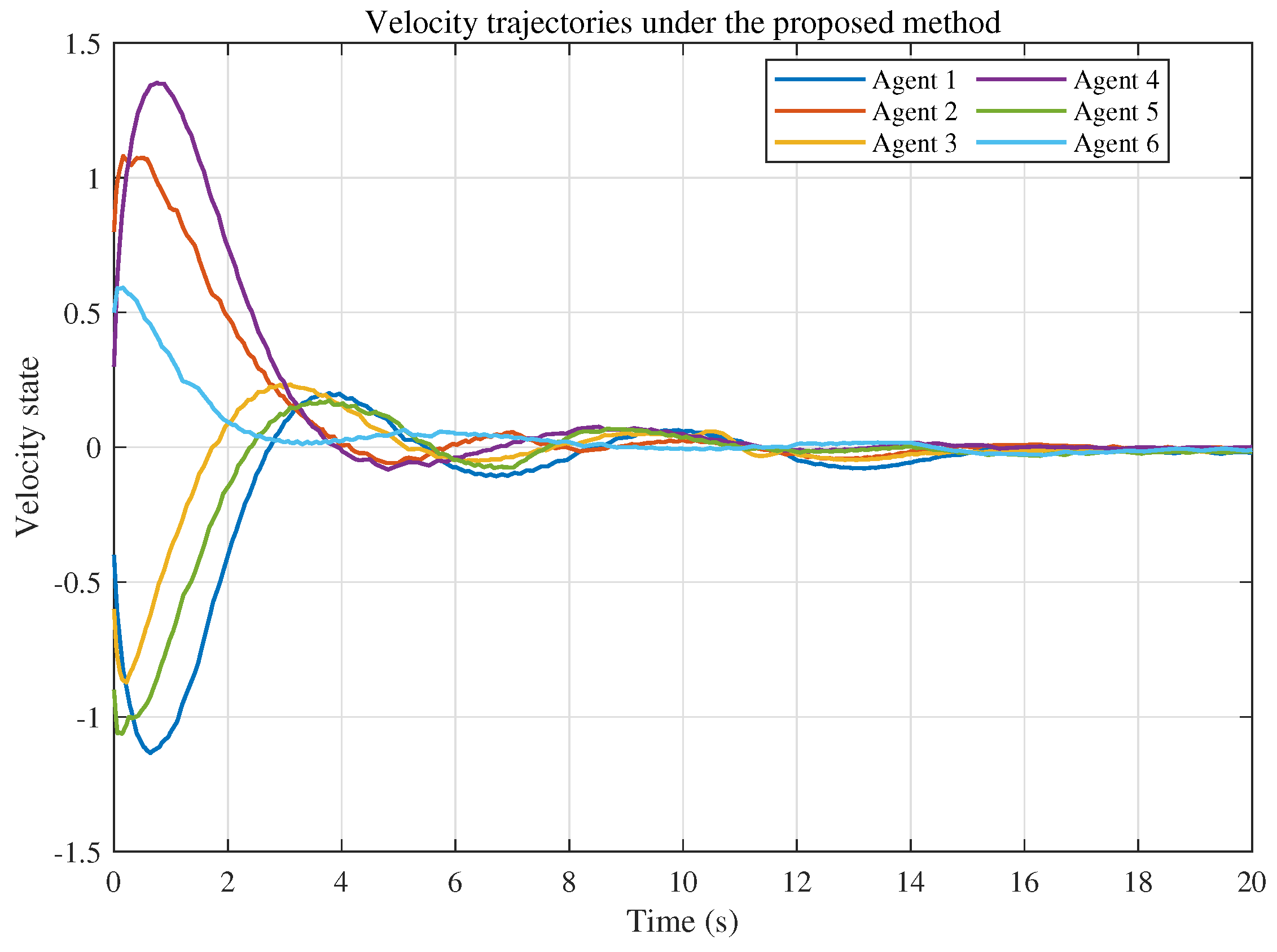
Figure 3 and Figure 4 show that the position and velocity disagreements decay despite heterogeneous initial states and disturbances. Since the uncoupled model in (53) is not asymptotically stable, the convergence is generated by the cooperative controller rather than by autonomous decay.

Figure 3. Position-state trajectories under the proposed dynamic event-triggered method.

Figure 4. Velocity-state trajectories under the proposed dynamic event-triggered method.

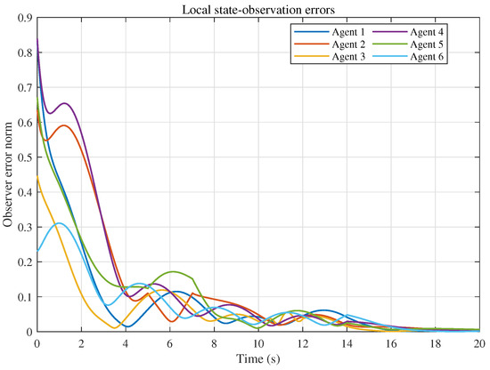
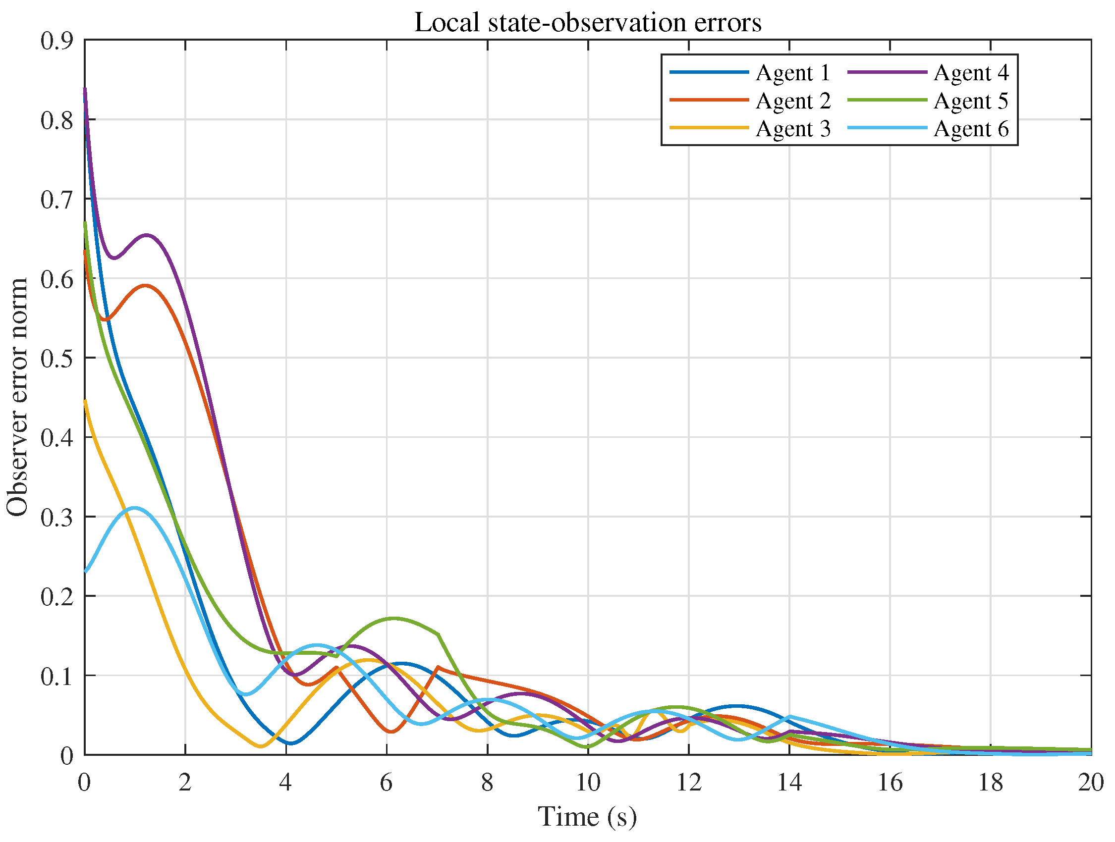
The observer-error norms in Figure 5 decrease rapidly and remain small during the disturbance intervals. The final network observer RMS is approximately $3.57\times {10}^{-3}$.

Figure 5. Norms of the local state-observation errors.

5.4. Communication Comparison and Adaptive Behavior

Four implementations are compared under identical plant dynamics, observer settings, disturbances, controller matrix, and initial conditions: the proposed dynamic trigger, the corresponding static trigger obtained by setting ${\eta }_i\equiv 0$, periodic broadcasting at every integration step, and a spectrum-dependent continuous observer baseline inspired by [23]. In the last case, current observer estimates are exchanged continuously and the fixed coupling is selected as $c_s=1/{\lambda }_2\left(L\right)$. This baseline represents the spectrum-dependent continuous-communication architecture associated with the closest fractional-order observer-based $H_{\infty }$ design.

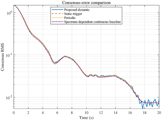
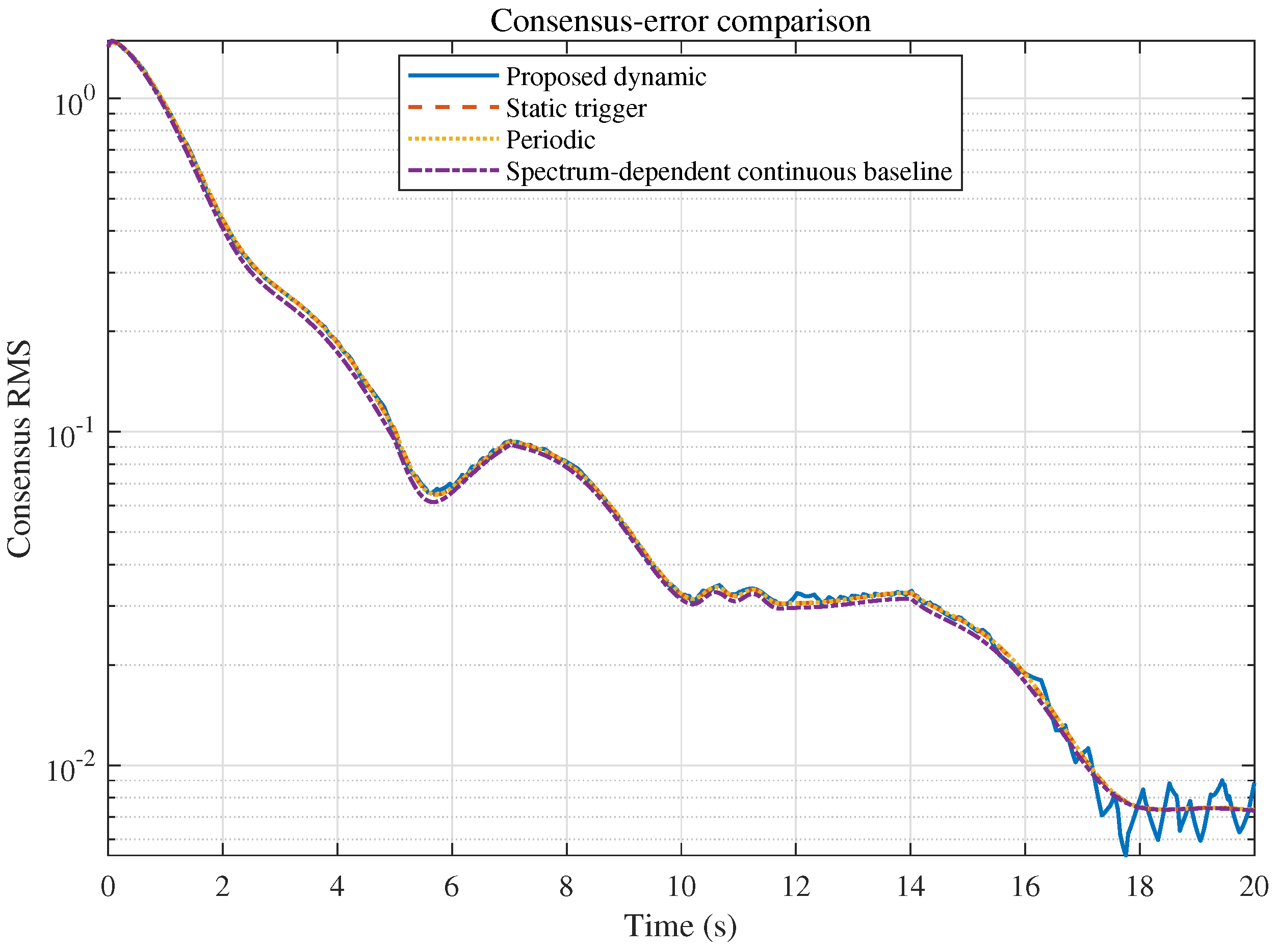
Figure 6 shows similar final consensus accuracy for all four methods. Table 3 reports the quantitative results. The energy ratio in this table includes nonzero initial disagreement and is therefore not interpreted as a strict induced norm.

Figure 6. Consensus RMS under the dynamic trigger, static trigger, periodic communication, and the spectrum-dependent continuous observer baseline.

Table 3. Core consensus and communication results.

Method	Transmissions	Final Consensus RMS	Final Observer RMS	Finite-Horizon Ratio	Peak $|{\mathit{u}}_{\mathit{i}}|$
Proposed dynamic trigger	366	0.00730	0.00357	5.040	4.340
Static trigger	3164	0.00734	0.00357	5.046	4.340
Periodic communication	6000	0.00735	0.00357	5.059	4.301
Spectrum-dependent continuous baseline	6000	0.00730	0.00357	4.934	7.168

Since Li et al. [23] is the closest fractional-order observer-based $H_{\infty }$ study, Figure 6 and Table 4 report a same-plant implementation comparison using the spectrum-dependent continuous observer baseline. Both implementations reach the same reported final consensus RMS, while the proposed method replaces continuous exchange and the global quantity ${\lambda }_2\left(L\right)$ with local adaptive couplings and event-triggered broadcasts.

Table 4. Same-plant numerical comparison with the spectrum-dependent continuous observer baseline.

Method	Graph Spectrum in Implementation	Communication	Transmissions	Final Consensus RMS	Finite-Horizon Ratio
Proposed dynamic trigger	No	Event-triggered	366	0.00730	5.040
Spectrum-dependent continuous observer baseline [23]	${\lambda }_2\left(L\right)$	Continuous	6000	0.00730	4.934

The comparison focuses on communication and closed-loop performance under the same plant and disturbance conditions. The proposed implementation uses $93.90\%$ fewer transmissions than the continuous baseline at the same final consensus RMS. The peak input is also lower for the proposed implementation ($4.340$ versus $7.168$), while the continuous baseline has a slightly smaller empirical finite-horizon energy ratio ($4.934$ versus $5.040$).

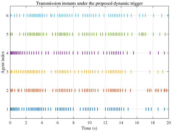
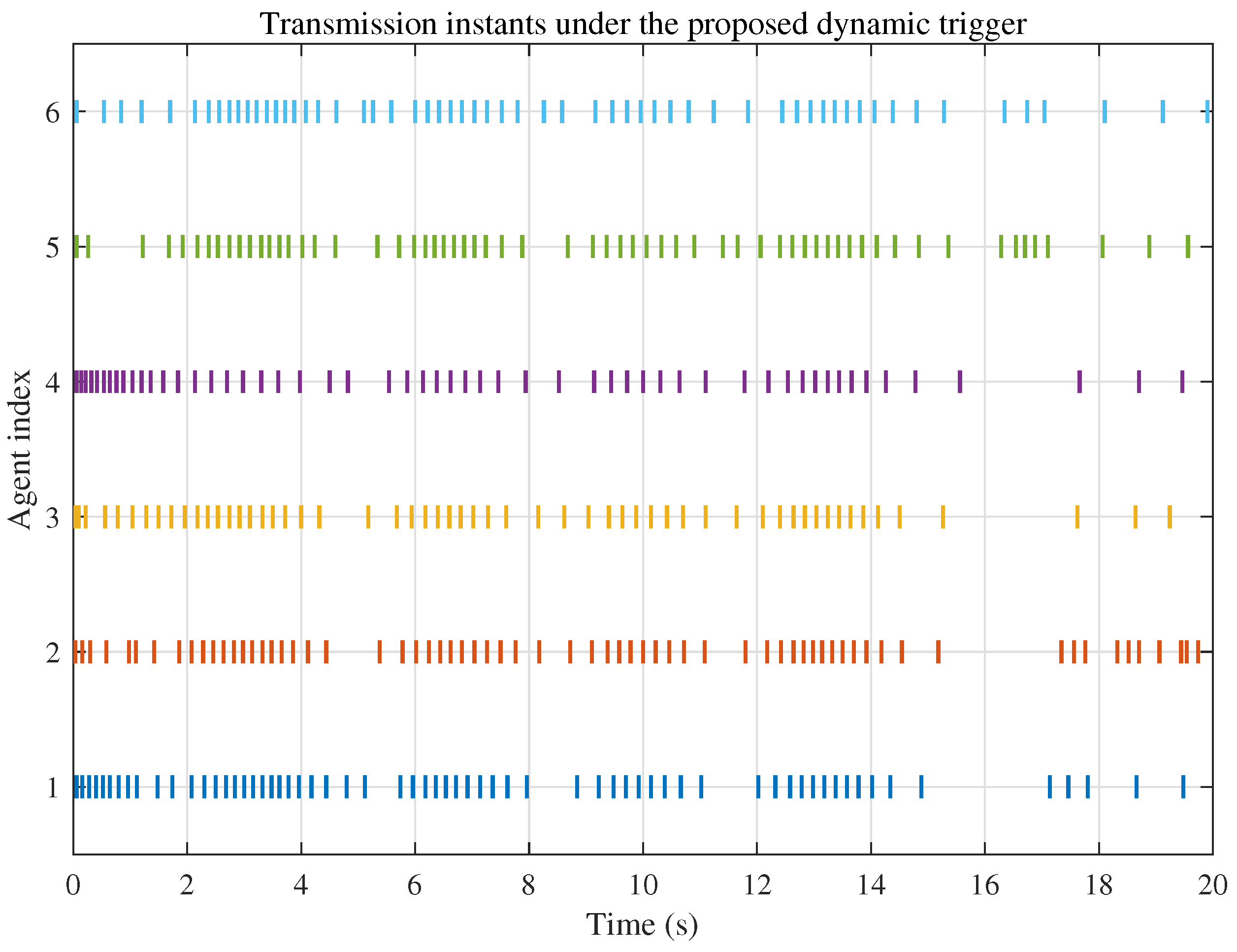
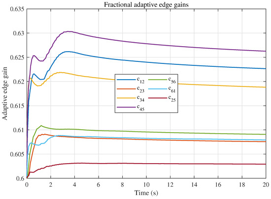
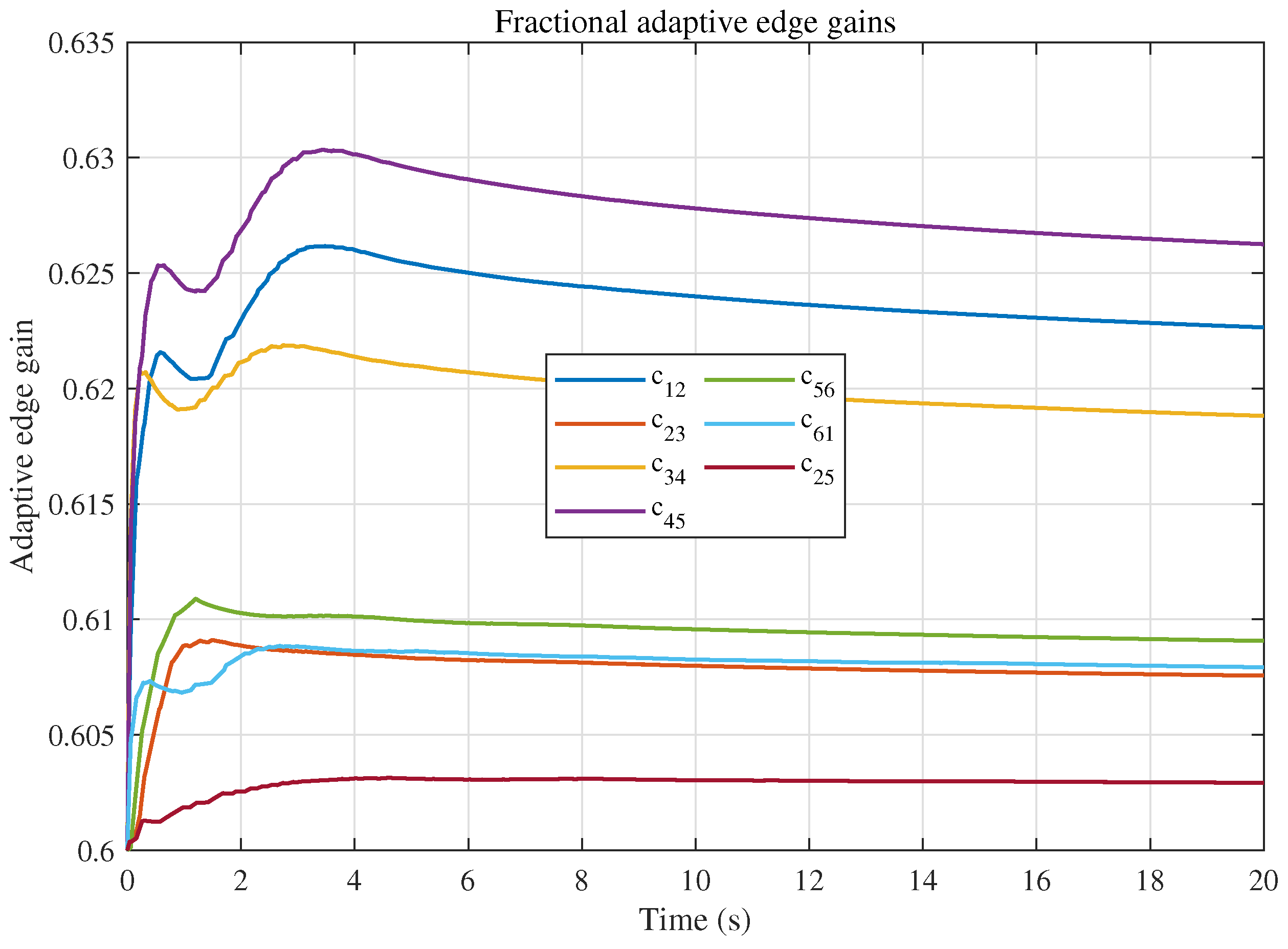
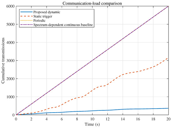
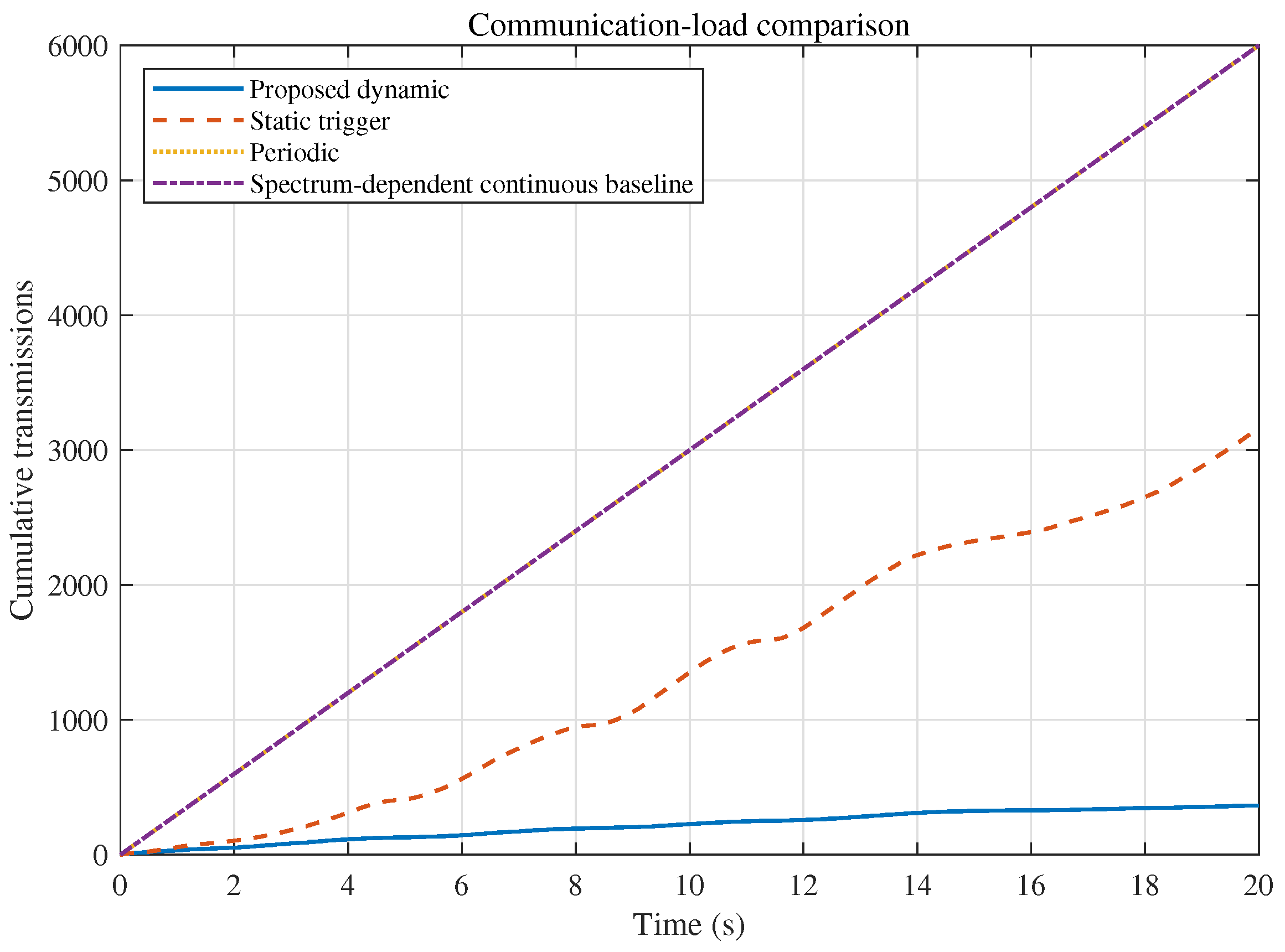
The proposed trigger reduces transmissions by $88.43\%$ relative to the static trigger and by $93.90\%$ relative to periodic communication. Figure 7 shows asynchronous, nonaccumulating transmission sequences. Figure 8 confirms that the fractional adaptive gains remain above their initial value and bounded; they are not claimed to be ordinarily monotone. The final gain range is approximately $0.603$–$0.626$.

Figure 7. Transmission instants of the six agents under the proposed dynamic trigger.

Figure 8. Fractional adaptive edge gains associated with the communication links.

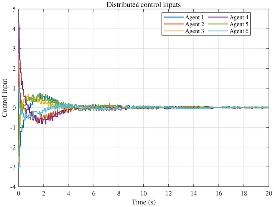
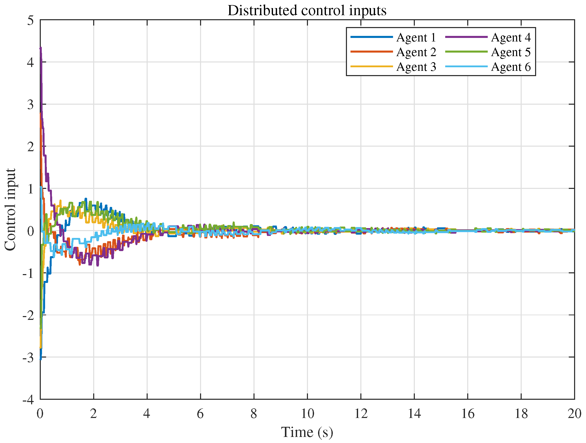
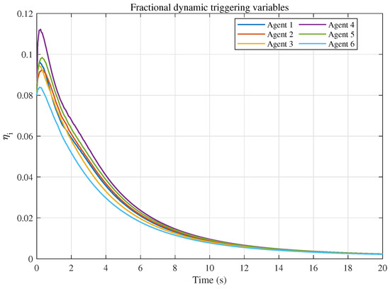
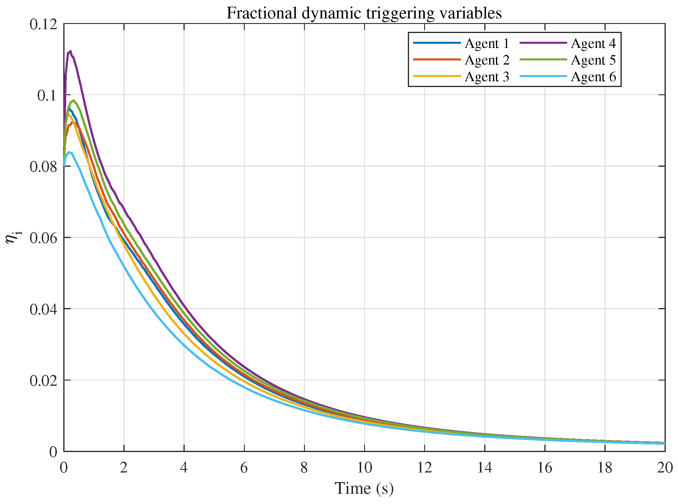
The inputs in Figure 9 remain bounded. Figure 10 shows positive internal trigger variables, while Figure 11 directly displays the communication saving.

Figure 9. Distributed control inputs under the proposed method.

Figure 10. Positive fractional dynamic variables used in the triggering conditions.

Figure 11. Cumulative transmissions for the four communication implementations.

5.5. Independent Disturbance-Attenuation Tests

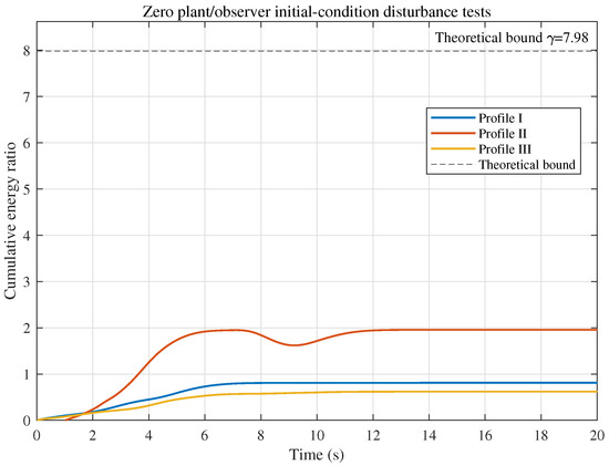
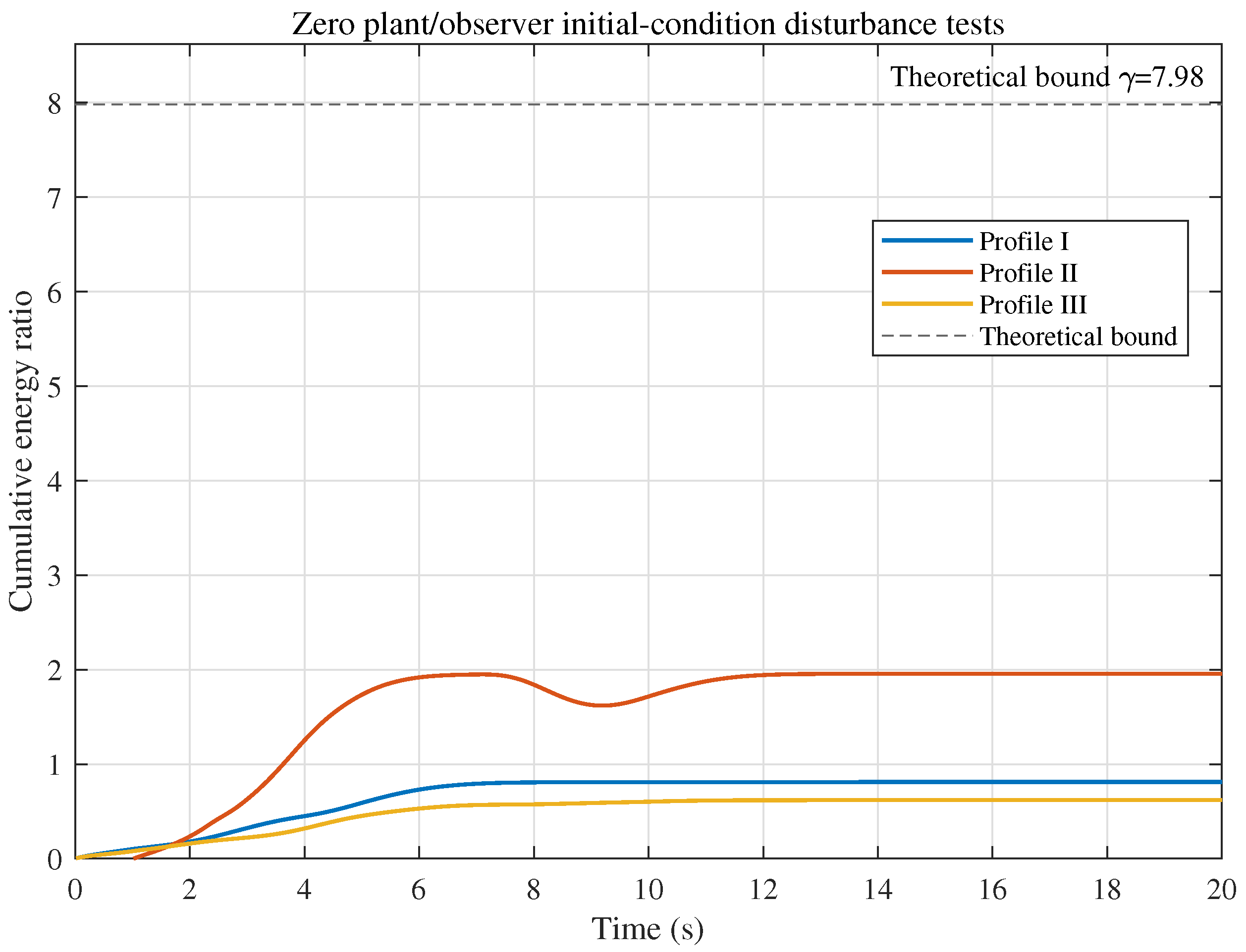
To separate disturbance energy from initial disagreement, three additional simulations use $x_i\left(0\right)={\widehat{x}}_i\left(0\right)=0$. The disturbance profiles are: an exponentially decaying multisine with a smooth pulse pair, two separated compact-support pulse pairs, and a damped two-frequency signal. Table 5 reports the empirical ratios

$$\widehat{\gamma }={\left({\displaystyle \frac{{\int }_0^{20}{z}_c^T{z}_{c}dt}{{\int }_0^{20}{w}^{T}wdt}}\right)}^{1/2}.$$

(60)

All empirical finite-horizon ratios are below $1.96$ and are therefore numerically consistent with the conservative composite attenuation bound $\gamma =7.98$. Since the adaptive gains and dynamic triggering variables have nonzero initial values, these ratios are reported as empirical performance indicators rather than as a direct numerical computation of the induced norm in Definition 1. Figure 12 shows the cumulative ratios.

Table 5. Zero-physical-initial-state finite-energy disturbance tests.

Disturbance Profile	Transmissions	$\widehat{\mathit{\gamma }}$	Final Consensus RMS	Peak $|{\mathit{u}}_{\mathit{i}}|$
Exponentially decaying multisine	426	0.811	0.00065	0.229
Separated smooth pulses	181	1.957	0.00337	0.224
Damped two-frequency signal	539	0.619	0.00056	0.233

Figure 12. Cumulative energy ratios for the three zero-initial-state disturbance profiles and the theoretical generalized attenuation bound.

5.6. Attenuation-Certificate Sweep

The attenuation levels ${\gamma }_c$, ${\gamma }_v$, and ${\gamma }_z$ enter the bounded-real certificates, not the implemented controller. Therefore, changing a candidate $\gamma$ does not by itself change a closed-loop trajectory. To address the sensitivity of the certificate, all three channel levels are scaled by a common factor $\rho$ while $P_c$, $P_v$, $P_z$, F, K, and the controller parameters are kept fixed. The corresponding composite candidate is

$$\gamma \left(\rho \right)={\rho }^2{\gamma }_c{\gamma }_v+\rho {\gamma }_z.$$

(61)

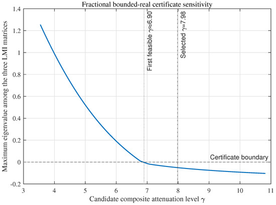
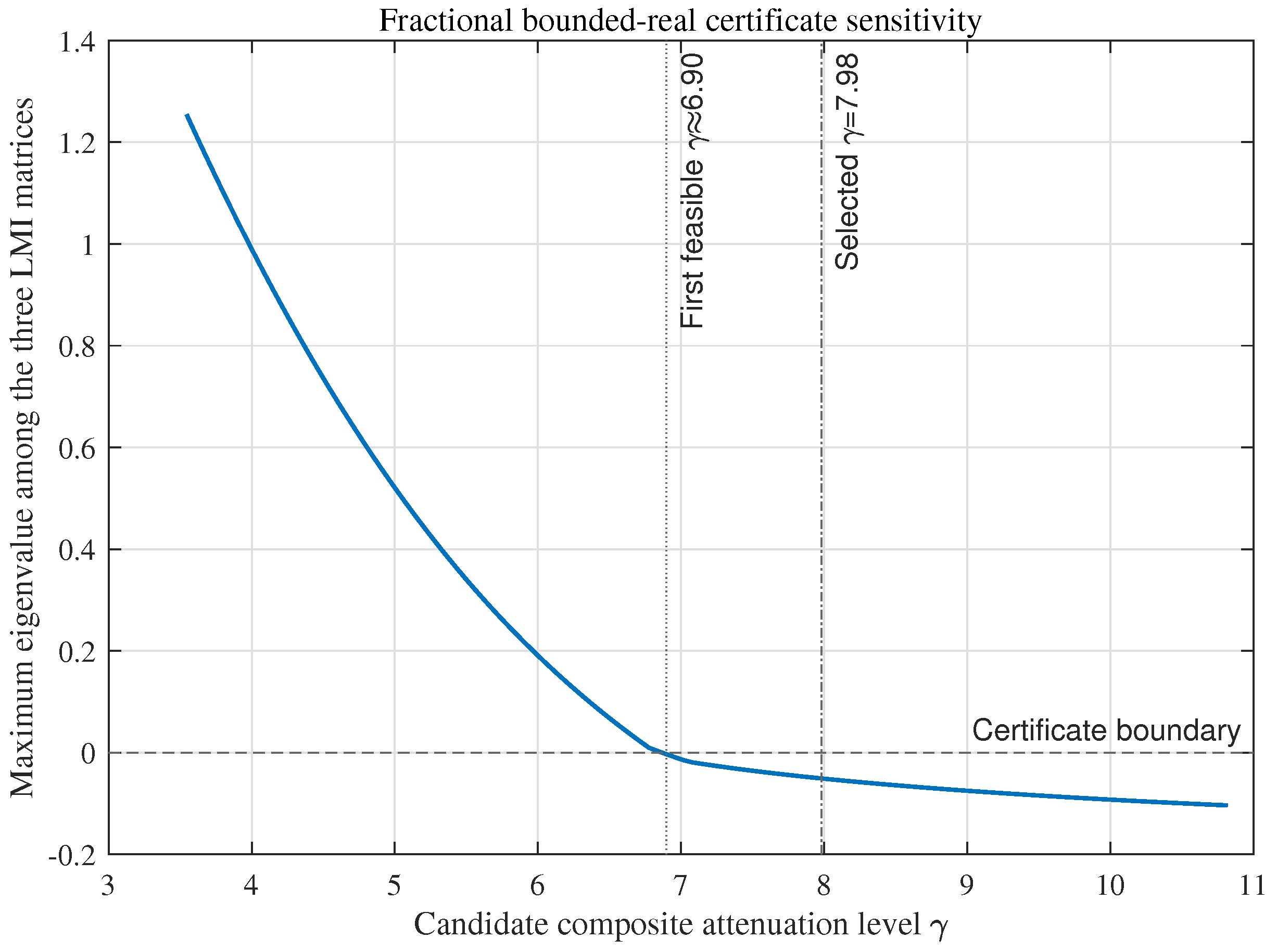
For each $\rho$, the maximum eigenvalue among the three fractional bounded-real matrices is recomputed. Figure 13 shows that the certificate becomes feasible when the composite candidate is approximately $6.90$ or larger, whereas the selected value $7.98$ has a clear negative-definiteness margin. For smaller candidates, the local LMIs lose feasibility, indicating that the corresponding attenuation level is not certified by Theorem 1. This loss of certificate does not imply closed-loop instability. The empirical disturbance ratios from Table 5 are shown only as trajectory-dependent references and remain conceptually distinct from the certified induced-gain bound.

Figure 13. Fractional bounded-real certificate margin versus the candidate composite attenuation level. Negative values indicate simultaneous feasibility of the three local LMIs.

5.7. Step-Size and Fractional-Order Sensitivity

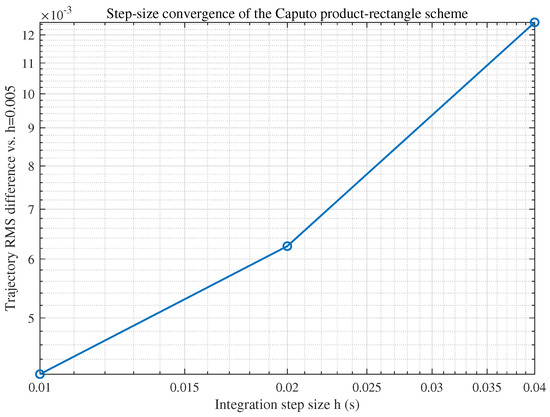
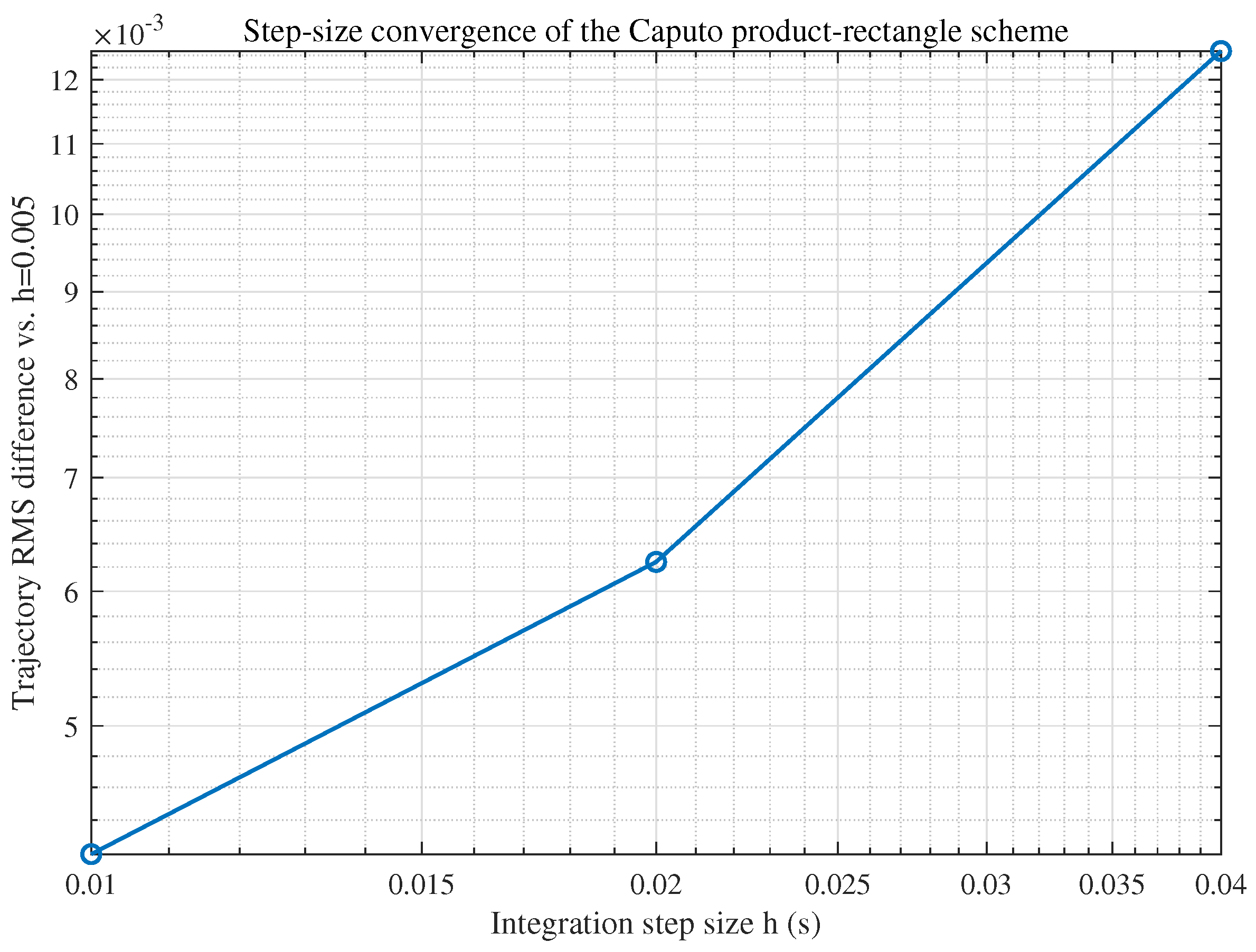
A step-size study is conducted using $h=0.005$ s as the reference. The trajectory RMS differences decrease from $1.25\times {10}^{-2}$ at $h=0.04$ s to $4.20\times {10}^{-3}$ at $h=0.01$ s, as shown in Figure 14. Table 6 also shows that the energy ratio varies by less than $0.7\%$ between $h=0.04$ and $h=0.005$.

Figure 14. Trajectory convergence with respect to the Caputo integration step size.

Table 6. Step-size sensitivity of the proposed simulation.

h (s)	Transmissions	Final Consensus RMS	Finite-Horizon Ratio	Trajectory RMS Difference
0.040	352	0.00602	5.0617	0.01247
0.020	366	0.00730	5.0404	0.00626
0.010	378	0.00947	5.0296	0.00420
0.005	387	0.00795	5.0283	0

The final consensus RMS does not vary monotonically with the integration step because grid-based event detection slightly shifts the triggering instants and hence the sampled closed-loop trajectory. Nevertheless, the trajectory-level RMS difference decreases with step refinement, while the finite-horizon energy ratio remains nearly unchanged, supporting numerical consistency.

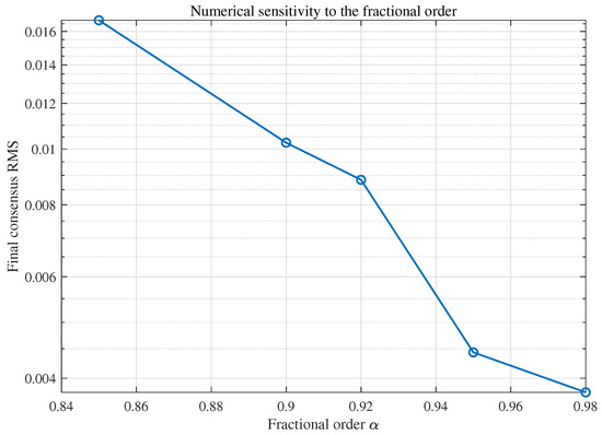
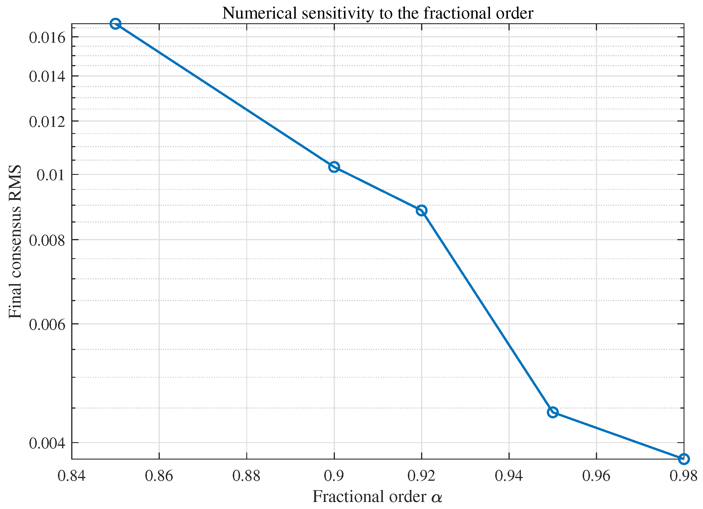
Finally, the same controller is evaluated numerically for $\alpha \in \{0.85,0.90,0.92,0.95,0.98\}$. The final consensus RMS remains below $1.83\times {10}^{-2}$ in all cases. Figure 15 reports the numerical sensitivity of the closed-loop response to the fractional order. The bounded-real certificate is evaluated at the nominal value $\alpha =0.92$; the remaining cases assess numerical sensitivity and are not covered by a common uncertain-order certificate.

Figure 15. Numerical sensitivity of the final consensus RMS to the fractional order; the bounded-real certificate is evaluated at the nominal order $\alpha =0.92$.

5.8. Application-Oriented Fractional Servo Synchronization

To examine applicability beyond the abstract benchmark, consider six electromechanical servo axes whose dominant position-loop dynamics exhibit memory effects. Fractional-order models have been investigated for armature-controlled DC servomotors [28], and fractional-order observer-based position control has been experimentally demonstrated on PMSM servo systems [29]. Motivated by these applications, a reduced fractional rigid-axis model is adopted for the coordination layer. Let ${\theta }_i$ denote the shaft angle, ${\omega }_i$ the generalized angular velocity, ${\tau }_i$ the actuator torque, and $d_i$ an external load torque. With representative equivalent inertia $J=0.8\mathrm{kg}{\mathrm{m}}^2$ and viscous damping $b=0.25\mathrm{N}\mathrm{m}\mathrm{s}/\mathrm{rad}$, a reference time scale ${\tau }_0>0$ is introduced so that the fractional derivative has the same physical dimension as an ordinary first derivative. The reduced model is written as

$${\tau }_0^{\alpha -1}{{}^{C}D}_t^{\alpha }{\theta }_i={\omega }_i,J{\tau }_0^{\alpha -1}{{}^{C}D}_t^{\alpha }{\omega }_i=-b{\omega }_i+{\tau }_i+d_i,y_i={\theta }_i.$$

(62)

With ${\tau }_0=1\mathrm{s}$ as the normalization time, the dimensional interpretation is explicit and the state-space representation becomes

$$A_s={\tau }_0^{1-\alpha }\left[\begin{array}{cc}0& 1\\ 0& -b/J\end{array}\right],B_s=E_s={\tau }_0^{1-\alpha }\left[\begin{array}{c}0\\ 1/J\end{array}\right].$$

(63)

For ${\tau }_0=1\mathrm{s}$, the matrices reduce numerically to the values used in the servo simulation. The fractional order, communication graph, trigger parameters, and storage matrices are kept consistent with the benchmark, while $K_s=B_s^T{P}_c$ and $Q_s=P_c{B}_s{B}_s^T{P}_c$ are computed according to the proposed design rule. The three local bounded-real matrices remain strictly feasible for this physical parameter set.

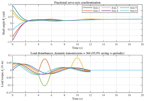
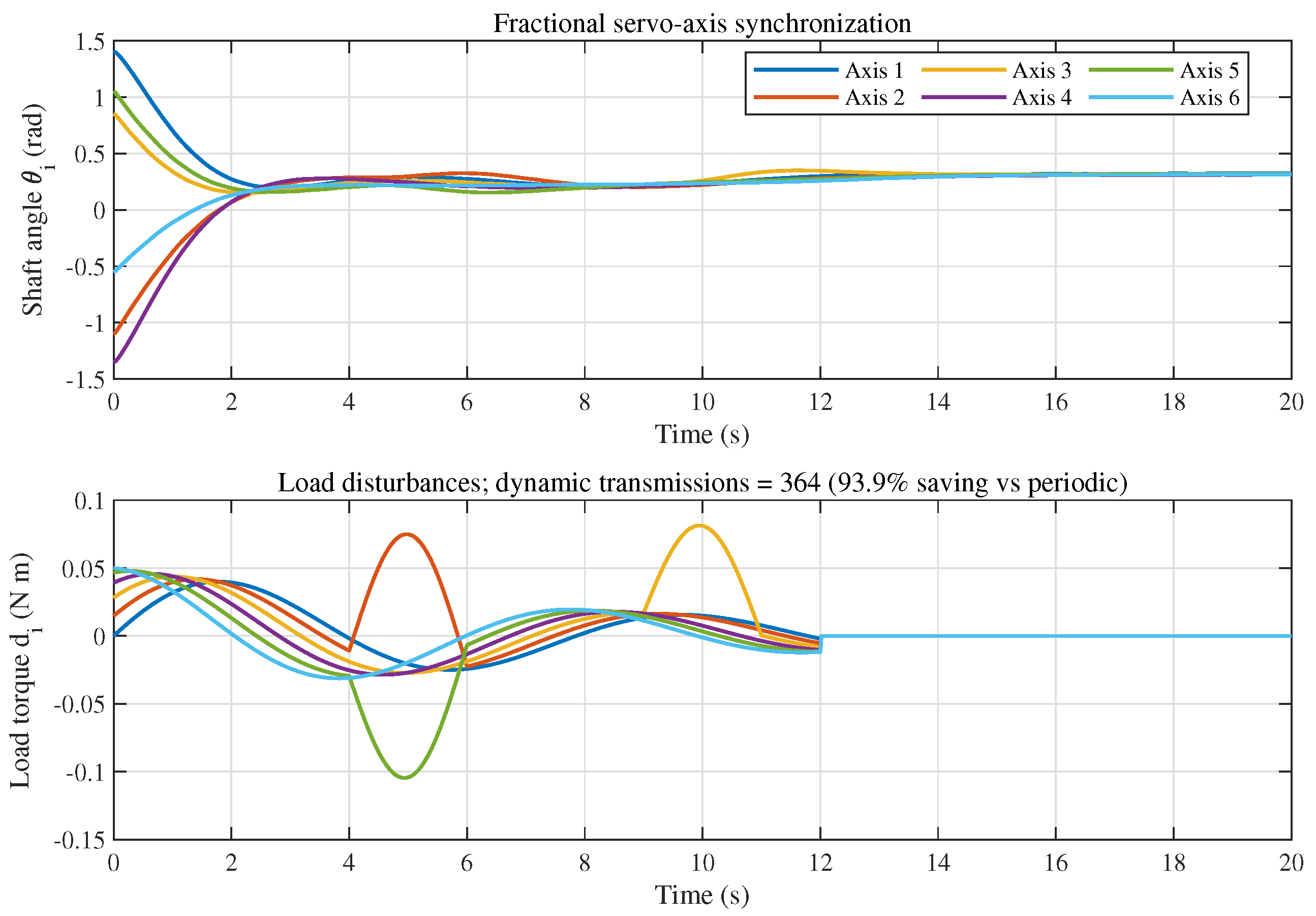
The six servo axes start from different angular positions and velocities and are subjected to a damped mechanical torque ripple together with finite-duration load-torque pulses on selected axes. Figure 16 shows that their shaft-angle trajectories synchronize after the disturbances while communication remains asynchronous. The representative run uses 364 transmissions versus 6000 under period-h broadcasting, i.e., approximately $6.1\%$ of the periodic communication load and a $93.9\%$ saving, with the final disagreement remaining below $8\times {10}^{-3}$. This example provides model-based validation of the proposed coordination strategy. Experimental evaluation with actuator saturation, nonlinear friction, parameter uncertainty, and identified fractional orders will be considered in future work.

Figure 16. Application-oriented fractional servo synchronization: shaft-angle responses and finite-duration load-torque disturbances under the proposed dynamic event-triggered controller.

6. Conclusions

A fully distributed dynamic event-triggered observer-based $H_{\infty }$ consensus method has been developed for linear fractional-order multi-agent systems. The explicit local trigger directly bounds the edge-weighted broadcast-error term, while fractional adaptive edge gains remove graph spectral information from implementation. The structural relation $K=B^T{P}_c$ guarantees that additional adaptive damping preserves the fractional bounded-real inequality. Three local performance channels yield the composite bound $\gamma ={\gamma }_c{\gamma }_v+{\gamma }_z$, and the positive fractional internal variable excludes finite event accumulation without imposing a prescribed dwell time. The simulations demonstrate substantial communication savings relative to static, periodic, and spectrum-dependent continuous observer baselines, while also verifying the bounded-real margins, disturbance attenuation, step-size sensitivity, off-nominal fractional-order sensitivity, and application-oriented servo performance. The present result is restricted to fixed connected undirected graphs, identical commensurate-order agents, and piecewise-continuous disturbances in ${\mathcal{L}}_2\cap {\mathcal{L}}_{\infty ,\mathrm{loc}}$; directed switching networks, heterogeneous or uncertain orders with a common certificate, actuator saturation, packet losses, and hardware experiments remain future topics.

References

- Podlubny, I. Fractional Differential Equations; Academic Press: San Diego, CA, USA, 1999. [Google Scholar]
- Diethelm, K. The Analysis of Fractional Differential Equations; Springer: Berlin/Heidelberg, Germany, 2010. [Google Scholar]
- Olfati-Saber, R.; Murray, R.M. Consensus problems in networks of agents with switching topology and time-delays. IEEE Trans. Autom. Control 2004, 49, 1520–1533. [Google Scholar] [CrossRef] [Scilit]
- Ren, W.; Beard, R.W. Consensus seeking in multiagent systems under dynamically changing interaction topologies. IEEE Trans. Autom. Control 2005, 50, 655–661. [Google Scholar] [CrossRef] [Scilit]
- Cao, Y.; Yu, W.; Ren, W.; Chen, G. An overview of recent progress in the study of distributed multi-agent coordination. IEEE Trans. Ind. Inform. 2013, 9, 427–438. [Google Scholar] [CrossRef] [Scilit]
- Zhu, W.; Chen, B.; Yang, J. Consensus of fractional-order multi-agent systems with input time delay. Fract. Calc. Appl. Anal. 2017, 20, 52–70. [Google Scholar] [CrossRef] [Scilit]
- Yu, Z.; Jiang, H.; Hu, C.; Yu, J. Necessary and sufficient conditions for consensus of fractional-order multiagent systems via sampled-data control. IEEE Trans. Cybern. 2017, 47, 1892–1901. [Google Scholar] [CrossRef] [Scilit] [PubMed]
- Gong, P.; Lan, W. Adaptive robust tracking control for uncertain nonlinear fractional-order multi-agent systems with directed topologies. Automatica 2018, 92, 92–99. [Google Scholar] [CrossRef] [Scilit]
- Hu, T.; He, Z.; Zhang, X.; Zhong, S. Leader-following consensus of fractional-order multi-agent systems based on event-triggered control. Nonlinear Dyn. 2020, 99, 2219–2232. [Google Scholar] [CrossRef] [Scilit]
- Xiao, P.; Gu, Z. Adaptive event-triggered consensus of fractional-order nonlinear multi-agent systems. IEEE Access 2022, 10, 213–220. [Google Scholar] [CrossRef] [Scilit]
- Wang, L.; Dong, J. Event-based distributed adaptive fuzzy consensus for nonlinear fractional-order multiagent systems. IEEE Trans. Syst. Man Cybern. Syst. 2022, 52, 5901–5912. [Google Scholar] [CrossRef] [Scilit]
- Dimarogonas, D.V.; Frazzoli, E.; Johansson, K.H. Distributed event-triggered control for multi-agent systems. IEEE Trans. Autom. Control 2012, 57, 1291–1297. [Google Scholar] [CrossRef] [Scilit]
- Nowzari, C.; Garcia, E.; Cortés, J. Event-triggered communication and control of networked systems for multi-agent consensus. Automatica 2019, 105, 1–27. [Google Scholar] [CrossRef] [Scilit]
- Yi, X.; Liu, K.; Dimarogonas, D.V.; Johansson, K.H. Dynamic event-triggered and self-triggered control for multi-agent systems. IEEE Trans. Autom. Control 2019, 64, 3300–3307. [Google Scholar] [CrossRef] [Scilit]
- Li, Z.; Liu, X.; Ren, W.; Xie, L. Distributed consensus of linear multi-agent systems with adaptive dynamic protocols. Automatica 2013, 49, 1986–1995. [Google Scholar] [CrossRef] [Scilit]
- Li, Z.; Ren, W.; Liu, X.; Fu, M. Consensus of multi-agent systems with general linear and Lipschitz nonlinear dynamics using distributed adaptive protocols. IEEE Trans. Autom. Control 2013, 58, 1786–1791. [Google Scholar] [CrossRef] [Scilit]
- Cheng, B.; Li, Z. Fully distributed event-triggered protocols for linear multiagent networks. IEEE Trans. Autom. Control 2019, 64, 1655–1662. [Google Scholar] [CrossRef] [Scilit]
- Li, X.; Tang, Y.; Karimi, H.R. Consensus of multi-agent systems via fully distributed event-triggered control. Automatica 2020, 116, 108898. [Google Scholar] [CrossRef] [Scilit]
- He, W.; Xu, B.; Han, Q.-L.; Qian, F. Adaptive consensus control of linear multiagent systems with dynamic event-triggered strategies. IEEE Trans. Cybern. 2020, 50, 2996–3008. [Google Scholar] [CrossRef] [Scilit] [PubMed]
- Xia, L.; Li, Q.; Song, R.; Feng, Y. Dynamic asynchronous edge-based event-triggered consensus of multi-agent systems. Knowl.-Based Syst. 2023, 272, 110531. [Google Scholar] [CrossRef] [Scilit]
- Feng, T.; Wang, Y.-E.; Liu, L.; Wu, B. Observer-based event-triggered control for uncertain fractional-order systems. J. Frankl. Inst. 2020, 357, 9423–9441. [Google Scholar] [CrossRef] [Scilit]
- Zhang, C.; Zhang, G.; Han, W.; Lv, X.; Shi, Z. Distributed fixed-time control for high-order multi-agent systems with FTESO and feasibility constraints. J. Frankl. Inst. 2024, 361, 107219. [Google Scholar] [CrossRef] [Scilit]
- Li, H.; Liu, S.; Meng, G.; Fan, Q. Dynamic observer-based H-Infinity consensus control of fractional-order multi-agent systems. IEEE Trans. Autom. Sci. Eng. 2025, 22, 12720–12729. [Google Scholar] [CrossRef] [Scilit]
- Liang, S.; Wei, Y.H.; Pan, J.W.; Gao, Q.; Wang, Y. Bounded real lemmas for fractional order systems. Int. J. Autom. Comput. 2015, 12, 192–198. [Google Scholar] [CrossRef] [Scilit]
- Dolk, V.S.; Borgers, D.P.; Heemels, W.P.M.H. Output-based and decentralized dynamic event-triggered control with guaranteed Lp-gain performance and Zeno-freeness. IEEE Trans. Autom. Control 2017, 62, 34–49. [Google Scholar] [CrossRef] [Scilit]
- Liu, D.; Yang, G.-H. Dynamic event-triggered control for linear time-invariant systems with L2-gain performance. Int. J. Robust. Nonlinear Control 2019, 29, 507–518. [Google Scholar] [CrossRef] [Scilit]
- Diethelm, K.; Ford, N.J.; Freed, A.D. A predictor–corrector approach for the numerical solution of fractional differential equations. Nonlinear Dyn. 2002, 29, 3–22. [Google Scholar] [CrossRef] [Scilit]
- Abro, K.A.; Gómez-Aguilar, J.F.; Khan, I.; Nisar, K.S. Role of modern fractional derivatives in an armature-controlled DC servomotor. Eur. Phys. J. Plus 2019, 134, 553. [Google Scholar] [CrossRef] [Scilit]
- Huang, J.; Ma, P.; Bao, G.; Gao, F.; Shi, X. Research on position servo system based on fractional-order extended state observer. IEEE Access 2020, 8, 102748–102756. [Google Scholar] [CrossRef] [Scilit]
Disclaimer/Publisher’s Note: The statements, opinions and data contained in all publications are solely those of the individual author(s) and contributor(s) and not of MDPI and/or the editor(s). MDPI and/or the editor(s) disclaim responsibility for any injury to people or property resulting from any ideas, methods, instructions or products referred to in the content. |
© 2026 by the authors. Licensee MDPI, Basel, Switzerland. This article is an open access article distributed under the terms and conditions of the Creative Commons Attribution (CC BY) license.