Bifurcation Structure and Chaos Control in a Discrete-Time Fractional Predator–Prey Model with Double Allee Effect

Abstract

This paper investigates a discrete-time fractional-order predator–prey model incorporating a double Allee effect in the prey population, derived from a fractional differential system via the piecewise constant argument method to capture both memory effects and density-dependent constraints. We establish the existence and local stability of all biologically meaningful equilibria and show that the interaction between fractional memory and the double Allee threshold significantly influences the stability of the coexistence state. Through the integration of linear stability analysis and center manifold reduction, we are able to obtain explicit conditions for Neimark–Sacker and period-doubling bifurcations. The system exhibits rich dynamics, including periodic oscillations, quasi-periodicity, and chaos. The double Allee effect plays a key role in shaping system stability. To suppress instability and chaotic behavior, feedback and hybrid control strategies are applied and shown to be effective. Numerical simulations are given to confirm the results obtained by the theoretical analysis and to show the transitions among different dynamical states, in which the fractional-order memory and multiple Allee effects play important roles.

1. Introduction

The predator–prey model has become a cornerstone in the mathematical analysis of ecological systems, describing the complex interactions between two mutually dependent species: predators and their prey. The classical predator–prey framework, introduced by Lotka and Volterra [1,2], forms the basis of many ecological studies. It has been widely used to analyze population oscillations, species coexistence, and extinction thresholds. In essence, the model predicts how the prey population grows in the absence of predation, while the predator population relies on the availability of prey for food and survival. This predator–prey relationship often leads to periodic changes in population density, a phenomenon that has been widely observed in nature. With the progress of ecological research, there has been development in the models as well, incorporating more biological processes such as prey refuge [3], fear responses [4], harvesting [5], cannibalism [6], and the Allee effect [7]. These advancements have greatly enriched the predator–prey framework, establishing it as a vital tool not only for interpreting fundamental mechanisms of species interactions but also for informing strategies related to biodiversity conservation and population management.

The Allee effect, named after ecologist W.C. Allee [8], is a biological phenomenon in which the per capita rate of increase of a population is a positive function of population density, especially at low densities. The positive density dependence is usually ascribed to processes such as mate location, mutual defense, group foraging, avoiding inbreeding, and social thermoregulation. Two forms of Allee effects have been found in ecological theory: the strong Allee effect [9,10,11], which imposes a critical population size below which the population is inevitably headed to extinction because of negative growth rates, and the weak Allee effect [12,13,14], in which the growth rate of the population is reduced at low densities but remains positive. The inclusion of the Allee effect in predator–prey models can drastically change the dynamical structure, potentially resulting in bi-stability, extinction thresholds, limit cycles, or chaotic dynamics. Specifically, when a prey population is subject to multiple simultaneous processes of Allee type, the system is said to display a double Allee effect [15,16,17]. This can occur due to the combination of various biological constraints, such as mate limitation and mutual predator defense. Recent biological and theoretical investigations have shown that the double Allee effect can drastically affect the predator–prey dynamics, potentially increasing the chances of population extinction, multi-stability, and complex bifurcation structures. Hence, the inclusion of a double Allee effect in mathematical models is not only biologically inspired but also necessary for a proper description of the thresholds and feedbacks that determine species persistence and extinction.

Several studies have explored the role of the Allee effect in predator–prey systems, and its importance has been confirmed. Sen et al. [18] analyzed a predator–prey system with an Allee effect in the numerical response of predators and found that this generally led to the destabilization of the coexistence equilibrium, resulting in complex bifurcation diagrams and even the extinction of predators due to environmental enrichment. Zeng and Yu [19] showed that the Allee effect in species could greatly change the dynamics of the system and make it possible to observe Hopf and Bogdanov–Takens bifurcations, which were not present in the system without the Allee effect, thus increasing the complexity of the system. Song [20] investigated a discrete predator–prey model with nonlinear Allee effects in both species and found that the Allee effect resulted in bifurcations, chaos, and multistability and also indicated that a moderate Allee effect in predators could result in the stabilization of dynamics. Gonzalez-Olivares et al. [21] investigated the effects of double Allee effects on the prey population and demonstrated that various expressions of the Allee effect could lead to different numbers of limit cycles, thereby illustrating the sensitivity of system behavior to mathematical formulation. Also, Xia and Li [22] investigated a discrete model with double Allee effects and demonstrated bifurcations due to transcritical and Neimark–Sacker (NS) bifurcations, as supported by numerical simulations that demonstrated complex behaviors. These works, therefore, underscored the important role of Allee effects, whether in prey, predators, or both, in determining the stability and dynamics of ecological systems.

Recently, fractional-order differential equations have emerged as powerful mathematical tools for describing real-world phenomena, particularly in biological systems. In contrast to classical integer-order models that depend only on the current state, fractional-order models incorporate memory and hereditary effects, which naturally arise in many biological processes [23,24]. Memory effects are especially important in ecological systems, where past interactions between prey and predators, such as previous encounters and environmental adaptations, can influence present dynamics. Owing to this property, fractional-order models are often considered more realistic and accurate than their integer-order counterparts.

Some authors have also explored the predator–prey dynamics through a fractional-order model, which considers memory-dependent phenomena. Li et al. [25] analyzed a fractional-order predator–prey model with a prey refuge and explored the existence and stability of equilibrium points, which were confirmed by simulations. Tang [26] studied a fractional-order model with group defense and discussed the existence and stability of equilibria and the existence of Hopf bifurcation with simulations to support the results. Singh et al. [27] studied a discrete fractional-order Leslie–Gower model and showed that varying the memory parameter and step size resulted in complex dynamics such as NS bifurcations and chaos. Sarkar and Mondal [28] investigated a fractional predator–prey model with combined harvesting and showed the existence, uniqueness, and stability of solutions and Hopf bifurcation and the effect of harvesting parameters via numerical simulation. The above-mentioned works demonstrate the efficiency of fractional models in understanding complex and memory-based ecological phenomena.

In the present study, we examine a predator–prey system with a double Allee effect in the prey, as described in [29], to explore the interplay between density-dependent limitations and predator pressure and memory-dependent dynamics in a fractional-order setting. The considered fractional-order system is given by

$$\left\{\begin{array}{c}{}^{c}D^{\alpha }x\left(t\right)=x\left(t\right)\left({\displaystyle \frac{r}{x\left(t\right)+a}}(1-{\displaystyle \frac{x\left(t\right)}{k}})(x\left(t\right)-m)-qy\left(t\right)\right),\hfill \\ {}^{c}D^{\alpha }y\left(t\right)=y\left(t\right)(px\left(t\right)-d).\hfill \end{array}\right.$$

(1)

In system (1), the variables $x\left(t\right)$ and $y\left(t\right)$ are the densities of the prey and predator populations at time t, respectively. The operator ${}^{c}D^{\alpha }$ is the Caputo fractional derivative of order $0<\alpha <1$, which captures memory effect of the system by taking into account the effect of the past states on the current rate of change. This means that the evolution of the populations depends not only on the current population states but also on their historical evolution. The parameter r is the intrinsic growth rate of the prey population in the absence of environmental limitations, while the parameter k is the carrying capacity, which is the maximum population size that the environment can support. The prey growth term ${\displaystyle \frac{r}{x+a}}\left(1-{\displaystyle \frac{x}{k}}\right)(x-m)$ incorporates a double Allee effect through two distinct density-dependent mechanisms. The factor $(x-m)$ represents an Allee-type threshold effect, where the population growth is reduced when the prey density is close to or below the threshold level m. In addition, the term ${\displaystyle \frac{1}{x+a}}$ introduces another density-dependent mechanism that further suppresses the effective growth rate when the prey density is small. Together, these two components act simultaneously to reduce population growth at low densities, thereby capturing the combined influence of multiple Allee-type effects.

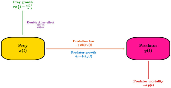
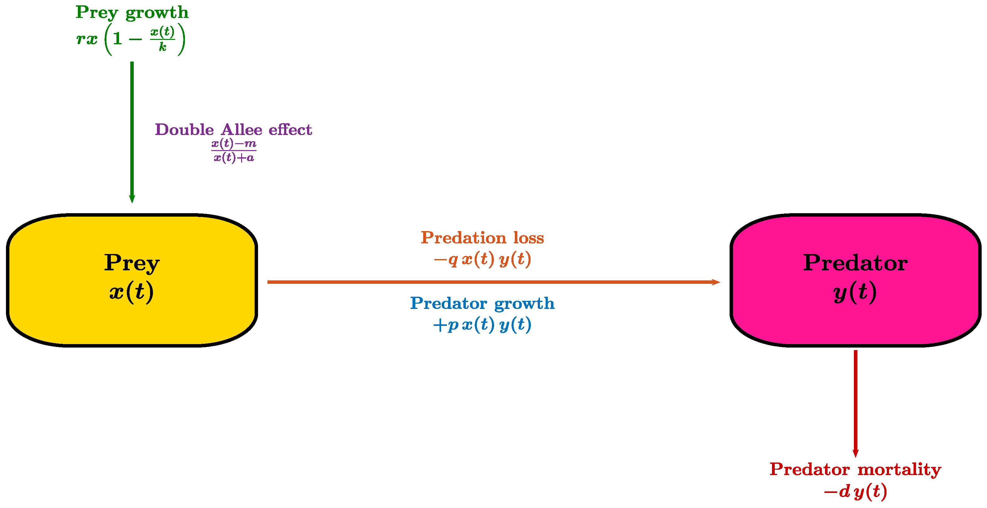
The parameter m is the Allee threshold, which is a critical level of population below which the prey may experience reduced growth or even go extinct because of factors such as the difficulty of finding mates or reduced cooperative behavior. The positive constant a is an auxiliary parameter in the modified growth term ${\displaystyle \frac{r}{x+a}}$, which not only ensures that the growth term remains bounded for small prey densities but also controls the intensity of the additional density-dependent suppression effect; biologically, it may represent environmental or behavioral limitations that reduce growth efficiency at low population densities. The parameter q denotes the predation rate coefficient, reflecting the intensity with which predators exploit the prey population, whereas p characterizes the conversion efficiency, indicating how effectively the ingested prey biomass contributes to predator growth or reproduction. The parameter d represents the natural mortality rate of the predator population in the absence of adequate food supply. The constraints $-k<m\le k$ ensure that the Allee threshold remains within ecologically meaningful limits in relation to the carrying capacity, while the condition $m>-a$ guarantees that the functional response term is well-defined for all biologically feasible values of the prey density. Figure 1 presents the flowchart of the system (1).

Figure 1. Flowchart of system (1).

Discrete-time models are particularly suitable for populations with non-overlapping generations, seasonal reproduction, or periodic harvesting, and they are well known for exhibiting rich dynamical behaviors such as bifurcations and chaos, even in low-dimensional settings. In ecological systems, such chaotic dynamics may result in irregular population oscillations or even species collapse. Since these fluctuations can threaten species persistence, the control of chaotic behavior has become an important topic in mathematical biology. Various control strategies have been developed to stabilize equilibria and regulate system dynamics, and can be interpreted as interventions aimed at maintaining ecological balance.

Several research studies have explored the complex dynamics of discrete fractional-order predator–prey models. Elsadany and Matouk [30] analyzed the fractional-order Lotka–Volterra model and its discrete version, illustrating that the discrete model has more complex dynamics, such as transcritical, flip, and NS bifurcations, and chaotic dynamics, compared to the continuous model, which only has stable or unstable equilibrium points. Mondal et al. [31] analyzed the fractional-order predator–prey model with habitat complexity and its discrete version, illustrating that the dynamics of the model are significantly affected by both the step size and the fractional order, resulting in bifurcations and chaotic dynamics. Uddin et al. [32] analyzed the discrete fractional-order model with harvesting and proved the existence of NS and period-doubling (PD) bifurcations and further applied chaos control methodologies to stabilize the model. Uddin and Podder [33] analyzed a prey–predator model with immigration, confirming the existence of bifurcations through center manifold and bifurcation theory, and used OGY and hybrid control to manage chaos. Ara and Rana [34] examined the stability and bifurcation behavior of a discrete model with the Caputo derivative, identifying strong resonances and applying control strategies to mitigate extreme instability. These studies demonstrate that discrete fractional-order models can capture complex dynamical behaviors that are not observed in their continuous counterparts.

While several studies have examined fractional-order predator–prey systems and their discrete counterparts, the incorporation of a double Allee effect within a discrete fractional framework remains underexplored. This motivates our investigation into the rich dynamical behavior of a discretized fractional-order predator–prey model with double Allee effects in the prey, using a piecewise constant argument method [35,36,37,38]. We discretize the system (1) using the piecewise constant approximation method as follows:

$$\left\{\begin{array}{c}{}^{c}D^{\alpha }x\left(t\right)=x\left(\left[{\displaystyle \frac{t}{h}}\right]h\right)\left({\displaystyle \frac{r}{x\left(\left[\frac{t}{h}\right]h\right)+a}}(1-{\displaystyle \frac{x\left(\left[\frac{t}{h}\right]h\right)}{k}})(x\left(\left[{\displaystyle \frac{t}{h}}\right]h\right)-m)-qy\left(\left[{\displaystyle \frac{t}{h}}\right]h\right)\right),\hfill \\ {}^{c}D^{\alpha }y\left(t\right)=y\left(\left[{\displaystyle \frac{t}{h}}\right]h\right)(px\left(\left[{\displaystyle \frac{t}{h}}\right]h\right)-d),\hfill \end{array}\right.$$

(2)

where $\left[{\displaystyle \frac{t}{h}}\right]$ represents the integer part of t within the interval $[nh,(n+1\left)h\right]$, with $n=0,$$1,2,\cdots ,$ and $h>0$ as the discretization parameter. The solution of the system (2) at the nth iteration is given by

$$\left\{\begin{array}{c}{x}_{n+1}\left(t\right)=x_n\left(nh\right)+{\displaystyle \frac{{(t-nh)}^{\alpha }}{\alpha \mathsf{\Gamma }\left(\alpha \right)}}{x}_n\left(nh\right)\left({\displaystyle \frac{r}{x_n\left(nh\right)+a}}(1-{\displaystyle \frac{x_n\left(nh\right)}{k}})(x_n\left(nh\right)-m)-q{y}_n\left(nh\right)\right),\hfill \\ y_{n+1}\left(t\right)=y_n\left(nh\right)+{\displaystyle \frac{{(t-nh)}^{\alpha }}{\alpha \mathsf{\Gamma }\left(\alpha \right)}}{y}_n\left(nh\right)(p{x}_n\left(nh\right)-d).\hfill \end{array}\right.$$

(3)

Letting $t\to (n+1)h$, (3) takes the form

$$\left\{\begin{array}{c}{x}_{n+1}=x_n+\mu x_n\left({\displaystyle \frac{r}{x_n+a}}(1-{\displaystyle \frac{x_n}{k}})(x_n-m)-q{y}_n\right),\hfill \\ y_{n+1}=y_n+\mu y_n(p{x}_n-d),\hfill \end{array}\right.$$

(4)

where $\mu ={\displaystyle \frac{h^{\alpha }}{\alpha \mathsf{\Gamma }\left(\alpha \right)}}$.

The discrete system (4) is obtained from the continuous fractional model (1) using the piecewise constant argument method, which assumes that the state variables remain constant over each interval $[nh,(n+1\left)h\right)$ for a sufficiently small step size. Compared with schemes, the piecewise constant argument method yields a simpler and computationally efficient discrete formulation while retaining the essential memory effects of the system. Moreover, this discretization preserves key qualitative properties, including positivity and equilibrium structure, and allows the study of complex dynamics such as bifurcations and chaos.

From a biological perspective, the Allee effect reduces prey growth at low population densities due to factors such as difficulty in finding mates, weakened cooperative defense, and inefficient resource use, which may lead to population decline even without strong predation. In the present model, the double Allee effect intensifies this behavior by introducing two density-dependent mechanisms that suppress growth at low densities, leading to critical thresholds below which extinction may occur. As a result, the Allee effect strongly influences the stability of equilibria, increases sensitivity to initial conditions, and determines whether the populations persist, oscillate, or collapse.

The main contributions of the paper are summarized as follows:

• We formulate a discrete-time fractional-order predator–prey model by incorporating a double Allee effect into a continuous-time system and then deriving its discrete counterpart using a fractional-order discretization scheme.
• We analyze the existence and stability of fixed points and identify how these are influenced by system parameters.
• We investigate bifurcation phenomena, including NS and PD bifurcations, using center manifold theory and bifurcation analysis techniques.
• Through detailed numerical simulations, we demonstrate the occurrence of complex dynamics such as periodic and quasi-periodic behavior, bifurcation and chaos.
• Finally, control strategies such as state feedback control and hybrid control are employed to suppress chaotic dynamics and promote stable long-term coexistence of the interacting species.

These contributions provide new perspectives on the role of the interaction between memory and double Allee effects in predator–prey systems. The findings of this study offer a more biologically realistic system for ecology and increase the set of tools for managing complex population dynamics.

Although fractional-order predator–prey models and Allee effects have been widely studied, most existing works focus either on continuous-time fractional systems or on discrete models with a single Allee effect. In contrast, the present study proposes a discrete fractional predator–prey model incorporating a double Allee effect, which introduces stronger low-density dependence and more complex threshold behavior. The main novelty of this work lies in this model formulation. Standard analytical tools, including stability analysis, bifurcation theory, and chaos control techniques, are then employed to investigate the dynamical properties of the proposed system.

The remainder of the paper is organized in the following way: The existence and topological classification of fixed points are examined in Section 2. The local bifurcations at the positive fixed point are studied in Section 3. Feedback and hybrid control methods are used in Section 4 to control bifurcations and reduce chaotic dynamics. Numerical simulations are presented in Section 5 to confirm the results obtained in the paper. Finally, the main conclusions of the paper are summarized in Section 6.

2. Existence and Stability of Fixed Points

This section examines the existence and local stability of the fixed points of the model. Fixed points are equilibrium solutions where the population densities of the interacting species are constant over time. The stability of fixed points offers insight into whether small changes in the population sizes tend to converge to the equilibrium solution or move away from the equilibrium solution.

2.1. Existence of Fixed Points

The fixed points $(\overline{x},\overline{y})$ of (4) represent steady states at which the population densities of both species remain constant over time. Thus, we solve the equations:

$$\left\{\begin{array}{c}\overline{x}=\overline{x}+\mu \overline{x}\left({\displaystyle \frac{r}{\overline{x}+a}}(1-{\displaystyle \frac{\overline{x}}{k}})(\overline{x}-m)-q\overline{y}\right),\hfill \\ \overline{y}=\overline{y}+\mu \overline{y}(p\overline{x}-d).\hfill \end{array}\right.$$

(5)

Solving (5) yields the following four fixed points:

$$E_0=(0,0),E_1=(k,0),E_2=(m,0),E_3=\left({\displaystyle \frac{d}{p}},{\displaystyle \frac{(kp-d)(d-mp)r}{kp(d+ap)q}}\right).$$

The equilibrium $E_0=(0,0)$ corresponds to the extinction state, where both species vanish, typically indicating an unfavorable environment. The boundary equilibrium $E_1=(k,0)$ represents the persistence of species x at its carrying capacity in the absence of species y, reflecting self-regulated growth. Similarly, $E_2=(m,0)$ describes the survival of species x at a low density determined by the Allee threshold, which is biologically meaningful only when $m>0$. The interior equilibrium $E_3=\left({\displaystyle \frac{d}{p}},{\displaystyle \frac{(kp-d)(d-mp)r}{kp(d+ap)q}}\right)$ characterizes the coexistence of both species, and its biological feasibility requires the condition $m<{\displaystyle \frac{d}{p}}<k$.

2.2. Classification of Fixed Points

To investigate the local behavior in the vicinity of each equilibrium, we evaluate the Jacobian matrix of (4) at $(\overline{x},\overline{y})$ as

$$J(\overline{x},\overline{y})=\left[\begin{array}{cc}1+{\displaystyle \frac{r(-akm+2a(k+m)\overline{x}+(-3a+k+m){\overline{x}}^2-2{\overline{x}}^3)\mu }{k{(a+\overline{x})}^2}}-q\overline{y}\mu & -q\overline{x}\mu \\ p\overline{y}\mu & 1-d\mu +p\overline{x}\mu \end{array}\right].$$

(6)

Let ${\theta }_1$ and ${\theta }_2$ denote eigenvalues of $J(\overline{x},\overline{y})$. The nature of each fixed point is determined according to the magnitudes of ${\theta }_1$ and ${\theta }_2$.

Definition 1. 

The fixed point $(\overline{x},\overline{y})$ is classified as follows:

1. 

A sink if ${\theta }_{1,2}$ satisfy $|{\theta }_{1,2}| < 1$, (${\theta }_{1,2}$ stands for: ${\theta }_1$ and ${\theta }_2$);

2. 

A source if the magnitudes of ${\theta }_1$ and ${\theta }_2$ are greater than 1;

3. 

A saddle if $max\left\{\right|{\theta }_1|,|{\theta }_2\left|\right\}>1$ and $min\left\{\right|{\theta }_1|,|{\theta }_2\left|\right\}<1$;

4. 

Non-hyperbolic if either $|{\theta }_1| = 1$ or $|{\theta }_2| = 1$.

While the above classification based on eigenvalues is standard, evaluating the eigenvalues explicitly can be cumbersome for complex Jacobians. To address this, we use the following criterion derived from the characteristic polynomial.

Lemma 1 

([39]). Let $\mathsf{\Delta }\left(\theta \right)={\theta }^2+K_1\theta +K_0$. Suppose that $\mathsf{\Delta }\left(1\right)>0$. If ${\theta }_1$ and ${\theta }_2$ are solutions of $\mathsf{\Delta }\left(\theta \right)=0$, then

1. 

$|{\theta }_1| < 1$ together with $|{\theta }_2| < 1$ if $\mathsf{\Delta }(-1)>0\wedge K_0<1$;

2. 

$|{\theta }_1| < 1 \wedge |{\theta }_2| > 1$ (or $|{\theta }_1| > 1 \wedge |{\theta }_2| < 1$) if $\mathsf{\Delta }(-1)<0$;

3. 

$|{\theta }_{1,2}| > 1$ if $\mathsf{\Delta }(-1)>0\wedge K_0>1$;

4. 

$|{\theta }_2| \ne 1$ and ${\theta }_1=-1$ if $\mathsf{\Delta }(-1)=0$ and $K_1\ne 0,2$;

5. 

${\theta }_1,{\theta }_2\in \mathbb{C}$ along with $|{\theta }_{1,2}| = 1$ if $K_1^2-4K_0<0\wedge K_0=1$.

The last two cases of Lemma 1 correspond to bifurcation phenomena commonly encountered in discrete dynamical systems:

• Case (4), where one eigenvalue equals $-1$ (i.e., ${\theta }_1=-1$) and the other does not lie on the unit circle (i.e., $|{\theta }_2| \ne 1$), signifies the occurrence of a PD bifurcation.
• Case (5), in which the eigenvalues are complex conjugates with modulus one (i.e., $|{\theta }_{1,2}| = 1$ and ${\theta }_{1,2}\in \mathbb{C}$), indicates the presence of an NS bifurcation.

These bifurcations indicate key changes in the qualitative dynamics of the system and play a crucial role in explaining the emergence of complex behaviors, including periodic oscillations and quasi-periodic motions.

Proposition 1. 

$E_0=(0,0)$ is

1. 

A sink if $0<m<k$ and $0<\mu <min\{{\displaystyle \frac{2a}{mr}},{\displaystyle \frac{2}{d}}\}$.

2. 

A source if any one of the following is satisfied:

a. 

$-k<m<0$ and $\mu >{\displaystyle \frac{2}{d}}$;

b. 

$0<m<k$ and $\mu >max\{{\displaystyle \frac{2a}{mr}},{\displaystyle \frac{2}{d}}\}$.

3. 

A saddle if any one of the following is satisfied:

a. 

$0<m<k$ and ${\displaystyle \frac{2}{d}}<\mu <{\displaystyle \frac{2a}{mr}}$;

b. 

$-k<m<0$ and $0<\mu <{\displaystyle \frac{2}{d}}$;

c. 

$0<m<k$ and ${\displaystyle \frac{2a}{mr}}<\mu <{\displaystyle \frac{2}{d}}$.

4. 

Non-hyperbolic if any one of the following is satisfied:

a. 

$m=0$;

b. 

$0<m<k$ and $\mu ={\displaystyle \frac{2a}{mr}}$;

c. 

$\mu ={\displaystyle \frac{2}{d}}$.

Proof. 

We obtain

$$J\left(E_0\right)=\left[\begin{array}{cc}1-{\displaystyle \frac{mr\mu }{a}}& 0\\ 0& 1-d\mu \end{array}\right].$$

(7)

The Jacobian matrix $J\left(E_0\right)$ has eigenvalues given by ${\theta }_1=1-{\displaystyle \frac{mr\mu }{a}}$ and ${\theta }_2=1-d\mu$. From the eigenvalue ${\theta }_2=1-d\mu$, we have

$$|1-d\mu |<1⟺-1<1-d\mu <1,$$

which yields $0<\mu <{\displaystyle \frac{2}{d}}$. Thus, we obtain

$$|1-d\mu |\left\{\begin{array}{c}<1,0<\mu <{\displaystyle \frac{2}{d}},\hfill \\ =1,\mu ={\displaystyle \frac{2}{d}},\hfill \\ >1,\mu >{\displaystyle \frac{2}{d}}.\hfill \end{array}\right.$$

(8)

Similarly, one can check that

$$|1-{\displaystyle \frac{mr\mu }{a}}|\left\{\begin{array}{c}<1,0<\mu <{\displaystyle \frac{2a}{mr}},0<m<k,\hfill \\ =1,m=0\mathrm{or}\mu ={\displaystyle \frac{2a}{mr}},0<m<k,\hfill \\ >1,-k<m<0\mathrm{or}\mu >{\displaystyle \frac{2a}{mr}},0<m<k.\hfill \end{array}\right.$$

(9)

□

Proposition 2. 

The fixed point located on the boundary, denoted by $E_1=(k,0)$, is

1. 

A sink if $-k<m<k,k<{\displaystyle \frac{d}{p}}$ and $0<\mu <min\{{\displaystyle \frac{2(a+k)}{(k-m)r}},{\displaystyle \frac{2}{d-kp}}\}$.

2. 

A source if any one of the following is satisfied:

a. 

$-k<m<k,k>{\displaystyle \frac{d}{p}}$ and $\mu >{\displaystyle \frac{2(a+k)}{(k-m)r}}$;

b. 

$-k<m<k,k<{\displaystyle \frac{d}{p}}$ and $\mu >max\{{\displaystyle \frac{2(a+k)}{(k-m)r}},{\displaystyle \frac{2}{d-kp}}\}$.

3. 

A saddle if any one of the following is satisfied:

a. 

$-k<m<k,k>{\displaystyle \frac{d}{p}}$ and $0<\mu <{\displaystyle \frac{2(a+k)}{(k-m)r}}$;

b. 

$-k<m<k,k<{\displaystyle \frac{d}{p}}$ and ${\displaystyle \frac{2}{d-kp}}<\mu <{\displaystyle \frac{2(a+k)}{(k-m)r}}$;

c. 

$-k<m<k,k<{\displaystyle \frac{d}{p}}$ and ${\displaystyle \frac{2(a+k)}{(k-m)r}}<\mu <{\displaystyle \frac{2}{d-kp}}$.

4. 

Non-hyperbolic if any one of the following is satisfied:

a. 

$m=k$;

b. 

$-k<m<k$ and $\mu ={\displaystyle \frac{2(a+k)}{(k-m)r}}$;

c. 

$k={\displaystyle \frac{d}{p}}$;

d. 

$k<{\displaystyle \frac{d}{p}}$ and $\mu ={\displaystyle \frac{2}{d-kp}}$.

Proof. 

We obtain

$$J\left(E_1\right)=\left[\begin{array}{cc}1+{\displaystyle \frac{(-k+m)r\mu }{a+k}}& -kq\mu \\ 0& 1-d\mu +kp\mu \end{array}\right].$$

(10)

The eigenvalues of $J\left(E_1\right)$ are ${\theta }_1=1+{\displaystyle \frac{(-k+m)r\mu }{a+k}}$ and ${\theta }_2=1-d\mu +kp\mu$. One can check that

$$|1+{\displaystyle \frac{(-k+m)r\mu }{a+k}}|\left\{\begin{array}{c}<1,0<\mu <{\displaystyle \frac{2(a+k)}{(k-m)r}},-k<m<k,\hfill \\ =1,m=k\mathrm{or}\mu ={\displaystyle \frac{2(a+k)}{(k-m)r}},-k<m<k,\hfill \\ >1,\mu >{\displaystyle \frac{2(a+k)}{(k-m)r}},-k<m<k.\hfill \end{array}\right.$$

(11)

Moreover,

$$|1-d\mu +kp\mu |\left\{\begin{array}{c}<1,0<\mu <{\displaystyle \frac{2}{d-kp}},k<{\displaystyle \frac{d}{p}},\hfill \\ =1,k={\displaystyle \frac{d}{p}}\mathrm{or}\mu ={\displaystyle \frac{2}{d-kp}},k<{\displaystyle \frac{d}{p}},\hfill \\ >1,k>{\displaystyle \frac{d}{p}}\mathrm{or}\mu >{\displaystyle \frac{2}{d-kp}},k<{\displaystyle \frac{d}{p}}.\hfill \end{array}\right.$$

(12)

□

Proposition 3. 

The fixed point located on the boundary, denoted by $E_2=(m,0)$, is

1. 

A sink if $0<m<min\{{\displaystyle \frac{d}{p}},k\}$ and $0<\mu <{\displaystyle \frac{2}{d-mp}}$.

2. 

Never a source.

3. 

A saddle if either of the following is satisfied:

a. 

${\displaystyle \frac{d}{p}}<m<k$;

b. 

$0<m<min\{{\displaystyle \frac{d}{p}},k\}$ and $\mu >{\displaystyle \frac{2}{d-mp}}$.

4. 

Non-hyperbolic if either of the following conditions holds:

a. 

$m=k$;

b. 

$m={\displaystyle \frac{d}{p}}$;

c. 

$0<m<{\displaystyle \frac{d}{p}}$ and $\mu ={\displaystyle \frac{2}{d-mp}}$.

Proof. 

We obtain

$$J\left(E_2\right)=\left[\begin{array}{cc}1+{\displaystyle \frac{m(1-\frac{m}{k})r\mu }{a+m}}& -mq\mu \\ 0& 1-d\mu +mp\mu \end{array}\right].$$

(13)

The eigenvalues of $J\left(E_1\right)$ are ${\theta }_1=1+{\displaystyle \frac{m(1-\frac{m}{k})r\mu }{a+m}}$ and ${\theta }_2=1-d\mu +mp\mu$. Since $0<m\le k$ for the existence of $E_2$, therefore ${\theta }_1\ge 1$. Moreover,

$$|1-d\mu +mp\mu |\left\{\begin{array}{c}<1,0<\mu <{\displaystyle \frac{2}{d-mp}},0<m<{\displaystyle \frac{d}{p}},\hfill \\ =1,m={\displaystyle \frac{d}{p}}\mathrm{or}\mu ={\displaystyle \frac{2}{d-mp}},0<m<{\displaystyle \frac{d}{p}},\hfill \\ >1,m>{\displaystyle \frac{d}{p}}\mathrm{or}\mu >{\displaystyle \frac{2}{d-mp}},0<m<{\displaystyle \frac{d}{p}}.\hfill \end{array}\right.$$

(14)

□

We now analyze the classification of the positive fixed point $E_3=\left({\displaystyle \frac{d}{p}},{\displaystyle \frac{(kp-d)(d-mp)r}{kp(d+ap)q}}\right)$ associated with model (4). The Jacobian matrix evaluated at $E_3$ is expressed as:

$$J\left({\displaystyle \frac{d}{p}},{\displaystyle \frac{(kp-d)(d-mp)r}{kp(d+ap)q}}\right)=\left[\begin{array}{cc}1+{\displaystyle \frac{d(-d^2-2adp+(km+a(k+m))p^2)r\mu }{kp{(d+ap)}^2}}& -{\displaystyle \frac{dq\mu }{p}}\\ {\displaystyle \frac{(-d+kp)(d-mp)r\mu }{k(d+ap)q}}& 1\end{array}\right].$$

(15)

$$\mathsf{\Delta }\left(\theta \right)={\theta }^2+K_1\theta +K_0,$$

where

$$\begin{array}{cc}\hfill K_1& =-2+{\displaystyle \frac{d(d^2+2adp-(km+a(k+m))p^2)r\mu }{kp{(d+ap)}^2}},\hfill \\ \hfill K_0& ={\displaystyle \frac{kp{(d+ap)}^2+d(-d^2-2adp+(km+a(k+m))p^2)r\mu -d(d+ap)(d-kp)(d-mp)r{\mu }^2}{kp{(d+ap)}^2}}.\hfill \end{array}$$

We then evaluate $\mathsf{\Delta }\left(1\right)$, $\mathsf{\Delta }(-1)$, and $K_0$, and use the conditions given in Lemma 1 to determine the location of eigenvalues relative to the unit circle. This allows us to classify the stability of the equilibrium and identify possible bifurcation scenarios. It can be obtained through calculations that

$$\begin{array}{cc}\hfill \mathsf{\Delta }\left(0\right)& ={\displaystyle \frac{kp{(d+ap)}^2+d(-d^2-2adp+(km+a(k+m))p^2)r\mu -d(d+ap)(d-kp)(d-mp)r{\mu }^2}{kp{(d+ap)}^2}},\hfill \\ \hfill \mathsf{\Delta }(-1)& ={\displaystyle \frac{4kp{(d+ap)}^2+2d(-d^2-2adp+(km+a(k+m))p^2)r\mu -d(d+ap)(d-kp)(d-mp)r{\mu }^2}{kp{(d+ap)}^2}},\hfill \\ \hfill \mathsf{\Delta }\left(1\right)& ={\displaystyle \frac{d(kp-d)(d-mp)r{\mu }^2}{kp(d+ap)}}.\hfill \end{array}$$

It is straightforward to verify that $\mathsf{\Delta }\left(1\right)>0$, hence the conditions of Lemma 1 are applicable. Thus, we obtain the following result.

Theorem 1. 

The positive fixed point $E_3=\left({\displaystyle \frac{d}{p}},{\displaystyle \frac{(kp-d)(d-mp)r}{kp(d+ap)q}}\right)$ of the model (4) is

1. 

A sink if ${\displaystyle \frac{kp{(d+ap)}^2+d(-d^2-2adp+(km+a(k+m))p^2)r\mu -d(d+ap)(d-kp)(d-mp)r{\mu }^2}{kp{(d+ap)}^2}}<1$ and

${\displaystyle \frac{4kp{(d+ap)}^2+2d(-d^2-2adp+(km+a(k+m))p^2)r\mu -d(d+ap)(d-kp)(d-mp)r{\mu }^2}{kp{(d+ap)}^2}}>0$;

2. 

A source if ${\displaystyle \frac{kp{(d+ap)}^2+d(-d^2-2adp+(km+a(k+m))p^2)r\mu -d(d+ap)(d-kp)(d-mp)r{\mu }^2}{kp{(d+ap)}^2}}>1$ and

${\displaystyle \frac{4kp{(d+ap)}^2+2d(-d^2-2adp+(km+a(k+m))p^2)r\mu -d(d+ap)(d-kp)(d-mp)r{\mu }^2}{kp{(d+ap)}^2}}>0$;

3. 

A saddle if ${\displaystyle \frac{4kp{(d+ap)}^2+2d(-d^2-2adp+(km+a(k+m))p^2)r\mu -d(d+ap)(d-kp)(d-mp)r{\mu }^2}{kp{(d+ap)}^2}}<0$;

4. 

Non-hyperbolic, and (4) undergoes a PD bifurcation at $E_3$ when

$-2+{\displaystyle \frac{d(d^2+2adp-(km+a(k+m))p^2)r\mu }{kp{(d+ap)}^2}}\ne 0,2$ and

$${\displaystyle \frac{4kp{(d+ap)}^2+2d(-d^2-2adp+(km+a(k+m))p^2)r\mu -d(d+ap)(d-kp)(d-mp)r{\mu }^2}{kp{(d+ap)}^2}}=0;$$

5. 

Non-hyperbolic, and (4) undergoes an NS bifurcation at $E_3$ when

$0<{\displaystyle \frac{d(d^2+2adp-(km+a(k+m))p^2)r\mu }{kp{(d+ap)}^2}}<4$ and

$${\displaystyle \frac{kp{(d+ap)}^2+d(-d^2-2adp+(km+a(k+m))p^2)r\mu -d(d+ap)(d-kp)(d-mp)r{\mu }^2}{kp{(d+ap)}^2}}=1.$$

3. Bifurcation Analysis

This section is devoted to an in-depth analysis of bifurcation phenomena, specifically focusing on PD and NS bifurcations at $E_3$. For a thorough analysis of bifurcation theory, interested readers are encouraged to refer to [40,41]. Bifurcations are extremely important for understanding the behavior of the system, as they show how small alterations in system parameters can cause drastic changes in the dynamics of predator–prey systems.

3.1. PD Bifurcation

The PD bifurcation is a primary mechanism through which a stable equilibrium loses stability and gives rise to periodic behavior. It is where a stable fixed point loses stability as an eigenvalue crosses $-1$ to give a periodic orbit of period two. The PD bifurcation is typically the first point in a series of events that can lead to chaos. In ecological systems, it represents the onset of a cycle of high and low population levels from one generation to the next, which can be linked to the observed cycles of species abundance. The identification and knowledge of PD bifurcations are therefore critical in determining long-term stability. In the present model, the emergence of PD bifurcation is strongly influenced by the interaction between the double Allee effect and memory. The double Allee effect introduces critical population thresholds at low densities, making the system more sensitive to perturbations, while the fractional-order memory incorporates the influence of past states. This combined effect can either delay or accelerate the loss of stability, thereby modifying the parameter regions where periodic oscillations arise.

We investigate PD bifurcation at $E_3$ based on case (4) as listed in Theorem 1. We can write

$${\displaystyle \frac{4kp{(d+ap)}^2+2d(-d^2-2adp+(km+a(k+m))p^2)r\mu -d(d+ap)(d-kp)(d-mp)r{\mu }^2}{kp{(d+ap)}^2}}=0$$

as

$$m={\displaystyle \frac{-4kp{(d+ap)}^2+2d(d^2+2adp-ak{p}^2)r\mu +d^2(d+ap)(d-kp)r{\mu }^2}{dpr\mu \left(2\right(a+k)p+(d+ap\left)\right(d-kp\left)\mu \right)}}.$$

This expression gives the critical value of the parameter m at which the eigenvalue becomes $-1$, indicating the onset of a period-doubling bifurcation. Introducing a small perturbation $\delta$ into m near the bifurcation value

$$m_{PD}={\displaystyle \frac{-4kp{(d+ap)}^2+2d(d^2+2adp-ak{p}^2)r\mu +d^2(d+ap)(d-kp)r{\mu }^2}{dpr\mu \left(2\right(a+k)p+(d+ap\left)\right(d-kp\left)\mu \right)}},$$

modifies system (4) as follows:

$$\left\{\begin{array}{c}{x}_{n+1}=x_n+\mu x_n\left({\displaystyle \frac{r}{x_n+a}}(1-{\displaystyle \frac{x_n}{k}})(x_n-(m_{PD}+\delta ))-q{y}_n\right),\hfill \\ y_{n+1}=y_n+\mu y_n(p{x}_n-d).\hfill \end{array}\right.$$

(16)

To shift the fixed point $E_3$ to $(0,0)$, we define

$$u_n=x_n-{\displaystyle \frac{d}{p}},v_n=y_n-{\displaystyle \frac{(kp-d)(d-(m_{PD}+\delta )p)r}{kp(d+ap)q}}.$$

Substituting these transformations into system (16) and expanding the resulting expressions in terms of $(u_n,v_n)$, we obtain a linear part given by the Jacobian matrix evaluated at $E_3$, together with higher-order nonlinear terms. This yields the following form:

$$\left[\begin{array}{c}{u}_{n+1}\\ v_{n+1}\end{array}\right]=\left[\begin{array}{cc}{\displaystyle \frac{2k(a+k)p^2+kp(d+ap)(-d+kp)\mu +d{(d-kp)}^{2}r{\mu }^2}{kp(-2(a+k)p+(d+ap\left)\right(-d+kp\left)\mu \right)}}& -{\displaystyle \frac{dq\mu }{p}}\\ {\displaystyle \frac{2(d-kp)(-2kp(d+ap)+d(d-kp\left)r\mu \right)}{dkq\left(2\right(a+k)p+(d+ap\left)\right(d-kp\left)\mu \right)}}& 1\end{array}\right]\left[\begin{array}{c}{u}_n\\ v_n\end{array}\right]+\left[\begin{array}{c}{\mathbb{F}}_1(u_n,v_n,\delta )\\ {\mathbb{F}}_2(u_n,v_n,\delta )\end{array}\right],$$

(17)

where

$$\begin{array}{cc}\hfill {\mathbb{F}}_1(u_n,v_n,\delta )& =a_1{u}_n^2+a_2{u}_n{v}_n+a_3{u}_n\delta +a_4{u}_n^3+a_5{u}_n^2\delta +O\left(4\right),\hfill \\ \hfill {\mathbb{F}}_2(u_n,v_n,\delta )& =b_1{u}_n{v}_n+b_2{u}_n\delta ,\hfill \end{array}$$

$$\begin{array}{cc}\hfill a_1& =-{\displaystyle \frac{4ak(a+k)p^3+2d^2(a+k)pr\mu +d(d-kp)(d^2+2adp-ak{p}^2)r{\mu }^2}{dk(d+ap)\left(2\right(a+k)p+(d+ap\left)\right(d-kp\left)\mu \right)}},a_2=-q\mu ,a_3={\displaystyle \frac{d(a+k)pr\mu }{k{(d+ap)}^2}},\hfill \end{array}$$

$$\begin{array}{cc}\hfill a_4& ={\displaystyle \frac{a(a+k)p^3(-dr\mu (2+d\mu )+kp(4+dr{\mu }^2))}{dk{(d+ap)}^2(2(a+k)p+(d+ap)(d-kp)\mu )}},a_5={\displaystyle \frac{a(a+k)p^{3}r\mu }{k{(d+ap)}^3}},b_1=p\mu ,b_2={\displaystyle \frac{p(d-kp)r\mu }{k(d+ap)q}}.\hfill \end{array}$$

To further simplify the system and separate the critical direction, we apply a linear transformation that converts the system into its canonical form. The canonical form of (17) can be obtained by using

$$\left[\begin{array}{c}{u}_n\\ v_n\end{array}\right]=\left[\begin{array}{cc}-{\displaystyle \frac{dkq(d^2\mu +kp(2-d\mu )+ap(2+d\mu -kp\mu ))}{(d-kp)(-2ak{p}^2+d^{2}r\mu -dkp(2+r\mu ))}}& -{\displaystyle \frac{dq\mu }{2p}}\\ 1& 1\end{array}\right]\left[\begin{array}{c}{e}_n\\ f_n\end{array}\right].$$

(18)

As a result, (17) is reduced to

$$\left[\begin{array}{c}{e}_{n+1}\\ f_{n+1}\end{array}\right]=\left[\begin{array}{cc}-1& 0\\ 0& \theta \end{array}\right]\left[\begin{array}{c}{e}_n\\ f_n\end{array}\right]+\left[\begin{array}{c}{\mathbb{G}}_1(e_n,f_n,\delta )\\ {\mathbb{G}}_2(e_n,f_n,\delta )\end{array}\right],$$

(19)

where

$$\theta ={\displaystyle \frac{-2k(a+k)p^2+3kp(d+ap)(-d+kp)\mu +d{(d-kp)}^{2}r{\mu }^2}{kp(-2(a+k)p+(d+ap\left)\right(-d+kp\left)\mu \right)}},$$

$$\begin{array}{cc}\hfill {\mathbb{G}}_1(e_n,f_n,\delta )& =c_1{e}_n^2+c_2{f}_n^2+c_3{e}_n{f}_n+c_4{e}_n\delta +c_5{f}_n\delta +c_6{e}_n^3+c_7{f}_n^3+c_8{e}_n^2{f}_n+c_9{e}_n^2\delta +c_{10}{e}_n{f}_n^2\hfill \\ \hfill & +c_{11}{f}_n^2\delta +c_{12}{e}_n{f}_n\delta +O\left(4\right),\hfill \\ \hfill {\mathbb{G}}_2(e_n,f_n,\delta )& =d_1{e}_n^2+d_2{f}_n^2+d_3{e}_n{f}_n+d_4{e}_n\delta +d_5{f}_n\delta +d_6{e}_n^3+d_7{f}_n^3+d_8{e}_n^2{f}_n+d_9{e}_n^2\delta +d_{10}{e}_n{f}_n^2\hfill \\ \hfill & +d_{11}{f}_n^2\delta +d_{12}{e}_n{f}_n\delta +O\left(4\right).\hfill \end{array}$$

The coefficients $c_i$ and $d_j$ (given in Appendix A) are obtained by substituting the transformed variables into the system (17) and performing a Taylor expansion around $(0,0,0)$. Next, let $Q^C$ denote the center manifold of system (19) near the origin, within a small neighborhood of $\delta =0$. This manifold can be obtained by

$$Q^C=\left\{(e_n,f_n,\delta )\in {\mathbb{R}}_{+}^3|f_n=p_0\delta +p_1{e}_n^2+p_2{e}_n\delta +p_3{\delta }^2+O\left(3\right)\right\}.$$

Restricting the system to the center manifold reduces the dynamics to a one-dimensional map, which is sufficient to analyze the bifurcation behavior. Through computations, we obtain $p_0=0,p_1={\displaystyle \frac{d_1}{1-\theta }},p_2=-{\displaystyle \frac{d_4}{1+\theta }},p_3=0$. Consequently, (19) is restricted to center manifold $Q^C$ as

$$\begin{array}{cc}\hfill \tilde{F}:=e_{n+1}& =-e_n+c_1{e}_n^2+c_4{e}_n\delta +\left(c_6+{\displaystyle \frac{c_3{d}_1}{1-\theta }}\right)e_n^3+\left(c_9+{\displaystyle \frac{c_5{d}_1}{1-\theta }}-{\displaystyle \frac{c_3{d}_4}{1+\theta }}\right)e_n^2\delta -{\displaystyle \frac{c_5{d}_4}{1+\theta }}{e}_n{\delta }^2+O\left(4\right).\hfill \end{array}$$

(20)

The occurrence and nature of the PD bifurcation are determined by the following nondegeneracy conditions, which are derived from normal form theory. For the Function (20) to undergo a PD bifurcation, it is required that the following two values be nonzero:

$$\begin{array}{cc}\hfill l_1& ={\tilde{F}}_{\delta }{\tilde{F}}_{e_n{e}_n}+2{\tilde{F}}_{e_n\delta }{|}_{(0,0)}=2c_4,\hfill \end{array}$$

(21)

$$\begin{array}{cc}\hfill l_2& ={\displaystyle \frac{1}{2}}{\left({\tilde{F}}_{e_n{e}_n}\right)}^2+{\displaystyle \frac{1}{3}}{\tilde{F}}_{e_n{e}_n{e}_n}{|}_{(0,0)}=2\left(c_1^2+c_6+{\displaystyle \frac{c_3{d}_1}{1-\theta }}\right).\hfill \end{array}$$

(22)

Based on the above analysis and the derived nondegeneracy conditions, we state the following result.

Theorem 2. 

Consider that requirement (4) of Theorem 1 is fulfilled. Then (4) undergoes PD bifurcation at $E_3=\left({\displaystyle \frac{d}{p}},{\displaystyle \frac{(kp-d)(d-mp)r}{kp(d+ap)q}}\right)$ if $l_1,l_2$ given in (21) and (22) are non-zero and m varies in a small neighborhood of $m_{PD}={\displaystyle \frac{-4kp{(d+ap)}^2+2d(d^2+2adp-ak{p}^2)r\mu +d^2(d+ap)(d-kp)r{\mu }^2}{dpr\mu \left(2\right(a+k)p+(d+ap\left)\right(d-kp\left)\mu \right)}}$. Moreover, for positive values of $l_2$, the period-two orbits that bifurcate from $E_3$ are stable, and for negative values of $l_2$, these orbits are unstable.

3.2. NS Bifurcation

The NS bifurcation plays a crucial role in understanding how complex oscillatory dynamics emerge in discrete-time ecological systems. In particular, the onset of quasi-periodic behavior may correspond to persistent population cycles with non-repeating amplitudes, which are observed in real ecosystems. Detecting and controlling such bifurcations is therefore vital for maintaining ecological balance and avoiding erratic fluctuations in predator–prey interactions. In this model, the NS bifurcation is further influenced by the interaction between the double Allee effect and fractional-order memory, where the Allee effect strengthens nonlinear responses at low densities and memory effects modify the timing and persistence of oscillations, leading to quasi-periodic dynamics over a wider parameter range compared to classical models.

We investigate the NS bifurcation at $E_3=\left({\displaystyle \frac{d}{p}},{\displaystyle \frac{(kp-d)(d-mp)r}{kp(d+ap)q}}\right)$ when case (5) of Theorem 1 is satisfied. The NS bifurcation occurs when a pair of complex conjugate eigenvalues cross the unit circle. We can write

$${\displaystyle \frac{kp{(d+ap)}^2+d(-d^2-2adp+(km+a(k+m))p^2)r\mu -d(d+ap)(d-kp)(d-mp)r{\mu }^2}{kp{(d+ap)}^2}}=1$$

as

$$m={\displaystyle \frac{d^2+2adp-ak{p}^2+d(d+ap)(d-kp)\mu }{p\left(\right(a+k)p+(d+ap\left)\right(d-kp\left)\mu \right)}}.$$

To analyze the dynamics near the bifurcation point, we introduce a small perturbation parameter $\delta$ in m around its critical value $m_{NS}={\displaystyle \frac{d^2+2adp-ak{p}^2+d(d+ap)(d-kp)\mu }{p\left(\right(a+k)p+(d+ap\left)\right(d-kp\left)\mu \right)}}$, (4) is modified to

$$\left\{\begin{array}{c}{x}_{n+1}=x_n+\mu x_n\left({\displaystyle \frac{r}{x_n+a}}(1-{\displaystyle \frac{x_n}{k}})(x_n-(m_{NS}+\delta ))-q{y}_n\right),\hfill \\ y_{n+1}=y_n+\mu y_n(p{x}_n-d).\hfill \end{array}\right.$$

(23)

We introduce the transformation $u_n=x_n-{\displaystyle \frac{d}{p}},v_n=y_n-{\displaystyle \frac{(kp-d)(d-(m_{PD}+\delta )p)r}{kp(d+ap)q}}$ in order to shift $E_3$ to $(0,0)$. Under this mapping, the system (23) can be expressed as follows:

$$\left[\begin{array}{c}{u}_{n+1}\\ v_{n+1}\end{array}\right]=\left[\begin{array}{cc}{a}_{11}& -{\displaystyle \frac{dq\mu }{p}}\\ -{\displaystyle \frac{(d-kp)r\mu (-p\delta -\frac{(d + ap)(d - kp)}{(a + k)p + (d + ap)(d - kp)\mu })}{k(d+ap)q}}& 1\end{array}\right]\left[\begin{array}{c}{u}_n\\ v_n\end{array}\right]+\left[\begin{array}{c}{\mathbb{L}}_1(u_n,v_n)\\ {\mathbb{L}}_2(u_n,v_n)\end{array}\right],$$

(24)

where

$$\begin{array}{cc}\hfill a_{11}& =(-k(a+k)p^2{(d+ap)}^2+p(k{(d+ap)}^3(-d+kp)-d{(a+k)}^2{p}^{2}r\delta )\mu +d(d+ap)(-d+kp)r(-\left((d+ap)(d-kp)\right)\hfill \\ \hfill & +(a+k)p^2\delta ){\mu }^2)/\left(kp{(d+ap)}^2(-\left((a+k)p\right)+(d+ap)(-d+kp)\mu )\right),\hfill \end{array}$$

$$\begin{array}{cc}\hfill {\mathbb{L}}_1(u_n,v_n)& =a_1{u}_n^2+a_2{u}_n{v}_n+a_3{u}_n^3+O\left(4\right),\hfill \\ \hfill {\mathbb{L}}_2(u_n,v_n)& =p\mu u_n{v}_n,\hfill \end{array}$$

$$\begin{array}{cc}\hfill a_1& ={\displaystyle \frac{r\mu ((a+k)p(d{(d+ap)}^2-a(a+k)p^3\delta )+(d+ap)(-d+kp)(-\left((d+ap)(d^2+2adp-ak{p}^2)\right)+a(a+k)p^3\delta )\mu )}{k{(d+ap)}^3(-\left((a+k)p\right)+(d+ap)(-d+kp)\mu )}},\hfill \end{array}$$

$$\begin{array}{cc}\hfill a_2& =-q\mu ,a_3={\displaystyle \frac{a(a+k)p^{3}r\mu (d^2+2adp+a^2{p}^2+a{p}^2\delta +k{p}^2\delta +(d+ap)(d-kp)(d+p(a+\delta ))\mu )}{k{(d+ap)}^4(-\left((a+k)p\right)+(d+ap)(-d+kp)\mu )}}.\hfill \end{array}$$

To analyze the eigenvalues of the Jacobian matrix, we consider its characteristic equation given by

$${\theta }^2-P\left(\delta \right)\theta +Q\left(\delta \right)=0,$$

(25)

where

$$\begin{array}{cc}\hfill P\left(\delta \right)& =-(2a^{3}k{p}^4(1+d\mu -kp\mu )+d(k^2{p}^{3}r\delta \mu -d^{4}r{\mu }^2+2d^{3}kp\mu (1+r\mu )+d{k}^2{p}^2(2-pr\delta {\mu }^2)+d^{2}k{p}^2\mu (r\delta \mu \hfill \\ \hfill & -k(2+r\mu )\left)\right)+adp(-2d^{3}r{\mu }^2-2dkp(-1+kp\mu (3+r\mu ))+d^{2}p\mu (r\delta \mu +k(6+4r\mu ))+k{p}^2(2r\delta \mu +k(4\hfill \\ \hfill & -pr\delta {\mu }^2\left)\right))+a^2{p}^2(2k^2{p}^2-d^{3}r{\mu }^2+d^{2}p\mu (r\delta \mu +2k(3+r\mu ))-dp(-r\delta \mu +k^{2}p\mu (6+r\mu )+k(-4+pr\delta {\mu }^2))))\hfill \\ \hfill & /\left(kp{(d+ap)}^2(-d^2\mu +kp(-1+d\mu )+ap(-1-d\mu +kp\mu ))\right),\hfill \end{array}$$

$$\begin{array}{cc}\hfill Q\left(\delta \right)& ={\displaystyle \frac{a^{2}k{p}^2+d^{3}r\delta {\mu }^2+d^2(k+apr\delta {\mu }^2-kpr\delta {\mu }^2)+dp(ar\delta \mu +kr\delta \mu +ak(2-pr\delta {\mu }^2))}{k{(d+ap)}^2}}.\hfill \end{array}$$

The solutions of (25) are

$${\theta }_{1,2}={\displaystyle \frac{P\left(\delta \right)}{2}}\pm {\displaystyle \frac{i}{2}}\sqrt{4Q\left(\delta \right)-P^2\left(\delta \right)}.$$

(26)

We then obtain $|{\theta }_{1,2}|=\sqrt{Q\left(\delta \right)}$. Moreover,

$${\left({\displaystyle \frac{d|{\theta }_1|}{d\delta }}\right)}_{\delta =0}={\left({\displaystyle \frac{d|{\theta }_2|}{d\delta }}\right)}_{\delta =0}={\displaystyle \frac{dr\mu (d^2\mu +k(p-dp\mu )+ap(1+d\mu -kp\mu ))}{2k{(d+ap)}^2}}>0.$$

This transversality condition ensures that the eigenvalues cross the unit circle with nonzero speed, which is necessary for the occurrence of an NS bifurcation. Additionally, to avoid resonance cases, it is necessary that ${\theta }_{1,2}^i\ne 1$ for $i=1,2,3,4,$ when $\delta =0$, which is identical to the condition $P\left(0\right)\ne -2,0,-1,2$. By using the case (5) of Theorem 1, it follows that

$$P\left(0\right)={\displaystyle \frac{d^{3}r{\mu }^2+2ak{p}^2(-1-d\mu +kp\mu )-2d^{2}kp\mu (1+r\mu )+k^2{p}^2(-2+d\mu (2+r\mu ))}{kp(-d^2\mu +kp(-1+d\mu )+ap(-1-d\mu +kp\mu ))}}\ne \pm 2.$$

Therefore, we only require that

$$\begin{array}{c}\hfill P\left(0\right)={\displaystyle \frac{d^{3}r{\mu }^2+2ak{p}^2(-1-d\mu +kp\mu )-2d^{2}kp\mu (1+r\mu )+k^2{p}^2(-2+d\mu (2+r\mu ))}{kp(-d^2\mu +kp(-1+d\mu )+ap(-1-d\mu +kp\mu ))}}\ne 0,-1.\end{array}$$

(27)

To simplify the system and separate the rotational dynamics, we transform it into its canonical form. To derive the canonical form of (24) at $\delta =0$, we employ the following mapping

$$\left[\begin{array}{c}{u}_n\\ v_n\end{array}\right]=\left[\begin{array}{cc}-{\displaystyle \frac{dq\mu }{p}}& 0\\ -{\displaystyle \frac{d{(d-kp)}^{2}r{\mu }^2}{2kp(-d^2\mu +kp(-1+d\mu )+ap(-1-d\mu +kp\mu ))}}& -c_{22}\end{array}\right]\left[\begin{array}{c}{e}_n\\ f_n\end{array}\right],$$

(28)

where

$$\begin{array}{cc}\hfill c_{22}& ={\displaystyle \frac{1}{2}}\sqrt{-{\displaystyle \frac{d{(d-kp)}^{2}r{\mu }^2(d^{3}r{\mu }^2+4ak{p}^2(-1-d\mu +kp\mu )-2d^{2}kp\mu (2+r\mu )+k^2{p}^2(-4+d\mu (4+r\mu )))}{k^2{p}^2{(-d^2\mu +kp(-1+d\mu )+ap(-1-d\mu +kp\mu ))}^2}}}.\hfill \end{array}$$

Applying the transformation (28), system (24) is transformed as follows:

$$\left[\begin{array}{c}{e}_{n+1}\\ f_{n+1}\end{array}\right]=\left[\begin{array}{cc}{d}_{11}& -c_{22}\\ c_{22}& d_{22}\end{array}\right]\left[\begin{array}{c}{e}_n\\ f_n\end{array}\right]+\left[\begin{array}{c}\chi (e_n,f_n)\\ \mathsf{{\rm Y}}(e_n,f_n)\end{array}\right],$$

(29)

where

$$\begin{array}{cc}\hfill d_{11}& =d_{22}={\displaystyle \frac{d^{3}r{\mu }^2+2ak{p}^2(-1-d\mu +kp\mu )-2d^{2}kp\mu (1+r\mu )+k^2{p}^2(-2+d\mu (2+r\mu ))}{2kp(-d^2\mu +kp(-1+d\mu )+ap(-1-d\mu +kp\mu ))}},\hfill \end{array}$$

$$\begin{array}{cc}\hfill \chi (e_n,f_n)& =c_1{e}_n^2+c_2{e}_n{f}_n+c_3{e}_n^3+O\left(4\right),\hfill \end{array}$$

$$\begin{array}{cc}\hfill \mathsf{{\rm Y}}(e_n,f_n)& =d_1{e}_n^2+d_2{e}_n{f}_n+d_3{e}_n^3+O\left(4\right),\hfill \end{array}$$

$$\begin{array}{cc}\hfill c_1& ={\displaystyle \frac{dqr{\mu }^2(-2d(a+k)p-(d-kp)(d^2+d(3a+k)p-ak{p}^2)\mu )}{2kp(d+ap)(-((a+k)p)+(d+ap\left)\right(-d+kp\left)\mu \right)}},c_2=c_{22}q\mu ,\hfill \end{array}$$

$$\begin{array}{cc}\hfill c_3& ={\displaystyle \frac{a{d}^2(a+k)p{q}^{2}r{\mu }^3(1+d\mu -kp\mu )}{k{(d+ap)}^2(-\left((a+k)p\right)+(d+ap)(-d+kp)\mu )}},\hfill \end{array}$$

$$\begin{array}{cc}\hfill d_1& ={\displaystyle \frac{d^2{(d-kp)}^{2}qr{\mu }^4(2(a+k)p(kp(d+ap)+dr)+(d-kp)(2kp{(d+ap)}^2+(d^2+d(3a+k)p-ak{p}^2)r)\mu )}{4c_{22}{k}^2{p}^2(d+ap){((a+k)p+(d+ap)(d-kp)\mu )}^2}},\hfill \end{array}$$

$$\begin{array}{cc}\hfill d_2& ={\displaystyle \frac{dq{\mu }^2(2k(a+k)p^2+(d-kp)(2kp(d+ap)+(-d+kp)r)\mu )}{2kp(-((a+k)p)+(d+ap\left)\right(-d+kp\left)\mu \right)}},\hfill \end{array}$$

$$\begin{array}{cc}\hfill d_3& =-{\displaystyle \frac{a{d}^3(a+k){(d-kp)}^2{q}^2{r}^2{\mu }^5(1+d\mu -kp\mu )}{2c_{22}{k}^2{(d+ap)}^2{((a+k)p+(d+ap)(d-kp)\mu )}^2}}.\hfill \end{array}$$

In order to investigate the direction of NS bifurcation, we consider the first Lyapunov exponent, which is derived as follows [40,41]:

$$L={\left(\left[-Re\left({\displaystyle \frac{(1-2{\theta }_1){\theta }_2^2}{1-{\theta }_1}}{\tau }_{20}{\tau }_{11}\right)-{\displaystyle \frac{1}{2}}|{\tau }_{11}{|}^2-{\left|{\tau }_{02}\right|}^2+Re\left({\theta }_2{\tau }_{21}\right)\right]\right)}_{\delta =0},$$

(30)

where

$$\begin{array}{cc}\hfill {\tau }_{20}& ={\displaystyle \frac{1}{8}}\left[{\chi }_{e_n{e}_n}-{\chi }_{f_n{f}_n}+2{\mathsf{{\rm Y}}}_{e_n{f}_n}+i({\mathsf{{\rm Y}}}_{e_n{e}_n}-{\mathsf{{\rm Y}}}_{f_n{f}_n}-2{\chi }_{e_n{f}_n})\right],\hfill \\ \hfill {\tau }_{11}& ={\displaystyle \frac{1}{4}}\left[{\chi }_{e_n{e}_n}+{\chi }_{f_n{f}_n}+i({\mathsf{{\rm Y}}}_{e_n{e}_n}+{\mathsf{{\rm Y}}}_{f_n{f}_n})\right],\hfill \\ \hfill {\tau }_{02}& ={\displaystyle \frac{1}{8}}\left[{\chi }_{e_n{e}_n}-{\chi }_{f_n{f}_n}-2{\mathsf{{\rm Y}}}_{e_n{f}_n}+i({\mathsf{{\rm Y}}}_{e_n{e}_n}-{\mathsf{{\rm Y}}}_{f_n{f}_n}+2{\chi }_{e_n{f}_n})\right],\hfill \\ \hfill {\tau }_{21}& ={\displaystyle \frac{1}{16}}\left[{\chi }_{e_n{e}_n{e}_n}+{\chi }_{e_n{f}_n{f}_n}+{\mathsf{{\rm Y}}}_{e_n{e}_n{f}_n}+{\mathsf{{\rm Y}}}_{f_n{f}_n{f}_n}+i({\mathsf{{\rm Y}}}_{e_n{e}_n{e}_n}+{\mathsf{{\rm Y}}}_{e_n{f}_n{f}_n}-{\chi }_{e_n{e}_n{f}_n}-{\chi }_{f_n{f}_n{f}_n})\right].\hfill \end{array}$$

Based on the above analysis and the derived conditions, we obtain the following result.

Theorem 3. 

Suppose that case (5) of Theorem 1 is fulfilled. If requirement (27) holds and L given in (30) is nonzero, then (4) experiences NS bifurcation at $E_3=\left({\displaystyle \frac{d}{p}},{\displaystyle \frac{(kp-d)(d-mp)r}{kp(d+ap)q}}\right)$, as long as m changes in a small neighborhood of $m_{NS}={\displaystyle \frac{d^2+2adp-ak{p}^2+d(d+ap)(d-kp)\mu }{p\left(\right(a+k)p+(d+ap\left)\right(d-kp\left)\mu \right)}}$. Moreover, if $L<0$ (or $L>0$), the NS bifurcation at $E_3$ is identified as supercritical (or subcritical), and a unique closed invariant curve emerges from $E_3$, which is stable (or unstable).

4. Chaos Control

In this section, we explore two such methods: state feedback control and hybrid control. The state feedback control approach, inspired by the works in [42,43], is first applied to system (4) to curb its chaotic tendencies. Compared with other chaos control techniques, such as delayed feedback or impulsive control, this approach is relatively simple, relies only on current state information, and is both computationally efficient and suitable for practical implementation. This approach includes converting the original chaotic dynamics into a piecewise linear form, facilitating the design of an optimal controller aimed at minimizing an upper bound associated with the system’s behavior. The resulting optimization problem is addressed under specific constraints to ensure effective control. This technique is employed to stabilize chaotic orbits around an unstable equilibrium point of system (4). The corresponding controlled system is formulated as follows:

$$\left\{\begin{array}{c}{x}_{n+1}=x_n+\mu x_n\left({\displaystyle \frac{r}{x_n+a}}(1-{\displaystyle \frac{x_n}{k}})(x_n-m)-q{y}_n\right)-U_n,\hfill \\ y_{n+1}=y_n+\mu y_n(p{x}_n-d),\hfill \end{array}\right.$$

(31)

where $U_n={\kappa }_1\left(x_n-{\displaystyle \frac{d}{p}}\right)+{\kappa }_2\left(y_n-{\displaystyle \frac{(kp-d)(d-mp)r}{kp(d+ap)q}}\right)$ represents the feedback control term, with feedback gains ${\kappa }_1$ and ${\kappa }_2$ which are real numbers. From an ecological perspective, the feedback gains represent the strength of regulatory actions applied to the prey and predator populations, such as controlled harvesting or environmental interventions, which act to suppress large oscillations, stabilize population dynamics, and reduce the risk of extinction, thereby promoting sustainable coexistence. Next, we obtain

$$J\left({\displaystyle \frac{d}{p}},{\displaystyle \frac{(kp-d)(d-mp)r}{kp(d+ap)q}}\right)=\left[\begin{array}{cc}{\displaystyle \frac{-a^{2}k(-1+{\kappa }_1)p^3-d^{3}r\mu +d^{2}p(k-k{\kappa }_1-2ar\mu )+d{p}^2(amr\mu +kmr\mu +ak(2-2{\kappa }_1+r\mu ))}{kp{(d+ap)}^2}}& -{\displaystyle \frac{{\kappa }_{2}p+dq\mu }{p}}\\ {\displaystyle \frac{(-d+kp)(d-mp)r\mu }{k(d+ap)q}}& 1\end{array}\right].$$

(32)

The matrix $J\left({\displaystyle \frac{d}{p}},{\displaystyle \frac{(kp-d)(d-mp)r}{kp(d+ap)q}}\right)$ has the following characteristic equation:

$${\theta }^2+K_1\theta +K_0=0,$$

(33)

where

$$\begin{array}{cc}\hfill K_1& ={\displaystyle \frac{a^{2}k(-2+{\kappa }_1)p^3+d^{3}r\mu +d^{2}p(k(-2+{\kappa }_1)+2ar\mu )-d{p}^2(amr\mu +kmr\mu +ak(4-2{\kappa }_1+r\mu ))}{kp{(d+ap)}^2}},\hfill \\ \hfill K_0& ={\displaystyle \frac{1}{kp{(d+ap)}^{2}q}}(-d^{4}qr{\mu }^2-ak{p}^3(a(-1+{\kappa }_1)q+{\kappa }_{2}mpr\mu )-d^{3}r\mu ({\kappa }_{2}p+q(1+ap\mu -kp\mu -mp\mu ))\hfill \\ \hfill & +d{p}^2(km(-{\kappa }_{2}p+q)r\mu +a(k{\kappa }_{2}pr\mu +m({\kappa }_{2}p+q)r\mu +kq(2-2{\kappa }_1+r\mu -mpr{\mu }^2)))+d^{2}p\left(r\mu \right(-a{\kappa }_{2}p+{\kappa }_{2}mp\hfill \\ \hfill & +aq(-2+mp\mu ))+k({\kappa }_{2}pr\mu -q(-1+{\kappa }_1-apr{\mu }^2+mpr{\mu }^2))\left)\right).\hfill \end{array}$$

If ${\theta }_1$ and ${\theta }_2$ are the roots of (33), then we have

$$\begin{array}{cc}\hfill {\theta }_1+{\theta }_2& =-{\displaystyle \frac{a^{2}k(-2+{\kappa }_1)p^3+d^{3}r\mu +d^{2}p(k(-2+{\kappa }_1)+2ar\mu )-d{p}^2(amr\mu +kmr\mu +ak(4-2{\kappa }_1+r\mu ))}{kp{(d+ap)}^2}},\hfill \end{array}$$

(34)

$$\begin{array}{cc}\hfill {\theta }_1{\theta }_2& ={\displaystyle \frac{1}{kp{(d+ap)}^{2}q}}(-d^{4}qr{\mu }^2-ak{p}^3(a(-1+{\kappa }_1)q+{\kappa }_{2}mpr\mu )-d^{3}r\mu ({\kappa }_{2}p+q(1+ap\mu -kp\mu -mp\mu ))\hfill \\ \hfill & +d{p}^2(km(-{\kappa }_{2}p+q)r\mu +a(k{\kappa }_{2}pr\mu +m({\kappa }_{2}p+q)r\mu +kq(2-2{\kappa }_1+r\mu -mpr{\mu }^2)))+d^{2}p\left(r\mu \right(-a{\kappa }_{2}p\hfill \\ \hfill & +{\kappa }_{2}mp+aq(-2+mp\mu )) + k({\kappa }_{2}pr\mu -q(-1+{\kappa }_1-apr{\mu }^2+mpr{\mu }^2)\left)\right)).\hfill \end{array}$$

(35)

The boundaries of marginal stability are obtained by solving the conditions ${\theta }_1=\pm 1$ and ${\theta }_1{\theta }_2=1$. These criteria ensure that $|{\theta }_{1,2}| < 1$. Assuming that ${\theta }_1{\theta }_2=1$, it follows from Equation (35) that

$$L_1:-{\kappa }_1+\left({\displaystyle \frac{(-d+kp)(d-mp)r\mu }{k(d+ap)q}}\right){\kappa }_2+C_{10}=0,$$

(36)

where

$$C_{10}={\displaystyle \frac{dr\mu (-d^3\mu +d^2(-1-ap\mu +kp\mu +mp\mu )+dp(-kmp\mu +a(-2+kp\mu +mp\mu ))+p^2(km+a(k+m-kmp\mu )))}{kp{(d+ap)}^2}}.$$

Next, by setting ${\theta }_1=1$ and using Equations (34) and (35), we get

$$L_2:\left({\displaystyle \frac{(d-kp)(d-mp)r\mu }{k(d+ap)q}}\right){\kappa }_2+{\displaystyle \frac{d(d-kp)(d-mp)r{\mu }^2}{kp(d+ap)}}=0.$$

(37)

Next, by taking ${\theta }_1=-1$ and applying Equations (34) and (35), we derive

$$L_3:-2{\kappa }_1+\left({\displaystyle \frac{(-d+kp)(d-mp)r\mu }{k(d+ap)q}}\right){\kappa }_2+C_{30}=0,$$

(38)

where

$$\begin{array}{cc}\hfill C_{30}& ={\displaystyle \frac{1}{kp{(d+ap)}^2}}(4a^{2}k{p}^3-d^{4}r{\mu }^2+d^{3}r\mu (-2-ap\mu +kp\mu +mp\mu )+d^{2}p(ar\mu (-4+mp\mu )+k(4\hfill \\ \hfill & +apr{\mu }^2-mpr{\mu }^2\left)\right)+d{p}^2(2amr\mu +2kmr\mu +ak(8+r\mu (2-mp\mu )))).\hfill \end{array}$$

The stable eigenvalues are located inside the triangular region bounded by the curves $L_1,L_2$, and $L_3$.

We now apply the hybrid control approach introduced in [44] to regulate chaotic dynamics arising from both PD and NS bifurcations. This approach is particularly useful when single control mechanisms are not sufficient to suppress complex oscillations. This method combines state feedback with parameter modulation to stabilize unstable periodic orbits embedded within the chaotic attractor of the system. By combining both control mechanisms, the hybrid strategy provides greater adaptability and improved effectiveness in mitigating complex dynamical behavior. When applied to system (4), the controlled version of the model is given by

$$\left\{\begin{array}{c}{x}_{n+1}=\rho \left(x_n+\mu x_n\left({\displaystyle \frac{r}{x_n+a}}(1-{\displaystyle \frac{x_n}{k}})(x_n-m)-q{y}_n\right)\right)+(1-\rho )x_n,\hfill \\ y_{n+1}=\rho (y_n+\mu y_n(p{x}_n-d))+(1-\rho )y_n,\hfill \end{array}\right.$$

(39)

where $\rho \in (0,1)$ is the control parameter. Mathematically, $\rho$ determines the strength of the control action by balancing the original system dynamics and the controlled update. From an ecological perspective, it can be interpreted as the intensity of external intervention, such as partial harvesting or environmental regulation, applied at each time step to stabilize population fluctuations. The same fixed points are shared by (39) and (4). We obtain

$$J\left({\displaystyle \frac{d}{p}},{\displaystyle \frac{(kp-d)(d-mp)r}{kp(d+ap)q}}\right)=\left[\begin{array}{cc}{\displaystyle \frac{a^{2}k{p}^3-d^{3}r\mu \rho +d^{2}p(k-2ar\mu \rho )+d{p}^2(amr\mu \rho +kmr\mu \rho +ak(2+r\mu \rho ))}{kp{(d+ap)}^2}}& -{\displaystyle \frac{dq\mu \rho }{p}}\\ {\displaystyle \frac{(-d+kp)(d-mp)r\mu \rho }{k(d+ap)q}}& 1\end{array}\right],$$

(40)

and its characteristic equation is as follows:

$${\theta }^2+K_1\theta +K_0=0,$$

(41)

where

$$\begin{array}{cc}\hfill K_1& ={\displaystyle \frac{-2a^{2}k{p}^3+d^{3}r\mu \rho -2d^{2}p(k-ar\mu \rho )-d{p}^2(amr\mu \rho +kmr\mu \rho +ak(4+r\mu \rho ))}{kp{(d+ap)}^2}},\hfill \\ \hfill K_0& ={\displaystyle \frac{1}{kp{(d+ap)}^2}}(a^{2}k{p}^3-d^{4}r{\mu }^2{\rho }^2+d^{3}r\mu \rho (-1-ap\mu \rho +kp\mu \rho +mp\mu \rho )+d^{2}p(ar\mu \rho (-2+mp\mu \rho )\hfill \\ \hfill & +k(1+apr{\mu }^2{\rho }^2-mpr{\mu }^2{\rho }^2))+d{p}^2(amr\mu \rho +kmr\mu \rho +ak(2+r\mu \rho (1-mp\mu \rho )))).\hfill \end{array}$$

The positive fixed point $\left({\displaystyle \frac{d}{p}},{\displaystyle \frac{(kp-d)(d-mp)r}{kp(d+ap)q}}\right)$ of (39) is a sink if $|K_1| < 1+K_0<2$.

A limitation of the proposed control strategies is that they are model-based and rely on the system parameters and equilibrium values. In practice, these parameters are often estimated and may vary over time, which can influence the effectiveness of the control. Moreover, since the design is based on local stability analysis, the control performance may be limited for large perturbations or in the presence of external disturbances.

5. Numerical Simulations

In this section, we present numerical simulations to demonstrate the dynamic behavior of the fractional-order predator–prey model (4). The goal is to explore how varying key parameters influences the stability of equilibria and the emergence of bifurcations, particularly in the presence of memory effects introduced by the fractional-order formulation. The numerical computations are performed in Mathematica 13.3 due to its efficiency and accuracy in symbolic and numerical calculations, while MATLAB R2023b is used for graphical visualization because of its advanced and flexible plotting capabilities. The parameter values used in the simulations are hypothetical and are chosen to ensure biological feasibility and to illustrate the theoretical analysis. In particular, the selected parameters satisfy the conditions required for the existence of the interior equilibrium $E_3$ and the bifurcation conditions derived in Section 3. Moreover, certain parameters are varied systematically within specific ranges to capture transitions between stable, periodic, and chaotic dynamics, thereby confirming the analytical results.

5.1. NS Bifurcation Analysis Chaos Control

We investigate the occurrence of an NS bifurcation in (4) by varying the bifurcation parameter m, while keeping the other parameters fixed as $r=3.1,a=0.1,k=1.5,q=2.5,p=0.75,d=0.8,\mu =1.5$. For these values, the system undergoes an NS bifurcation at the critical value $m=m_{NS}\approx 0.576431$. The corresponding positive fixed point is $E_3\approx (1.066667,0.150526)$, and eigenvalues of $J\left(E_3\right)$ are ${\theta }_{1,2}=0.661317\pm 0.750106i$, satisfying the condition $\left|{\theta }_{1,2}\right|=1$. This verifies the onset of an NS bifurcation.

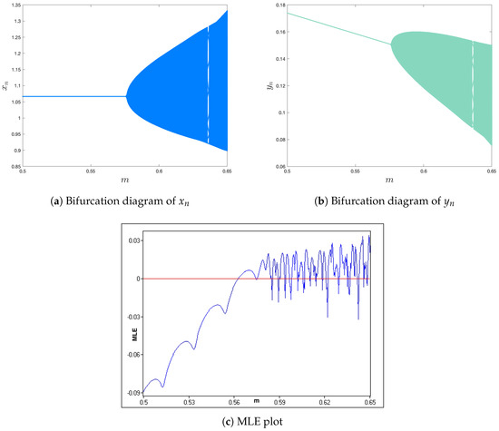
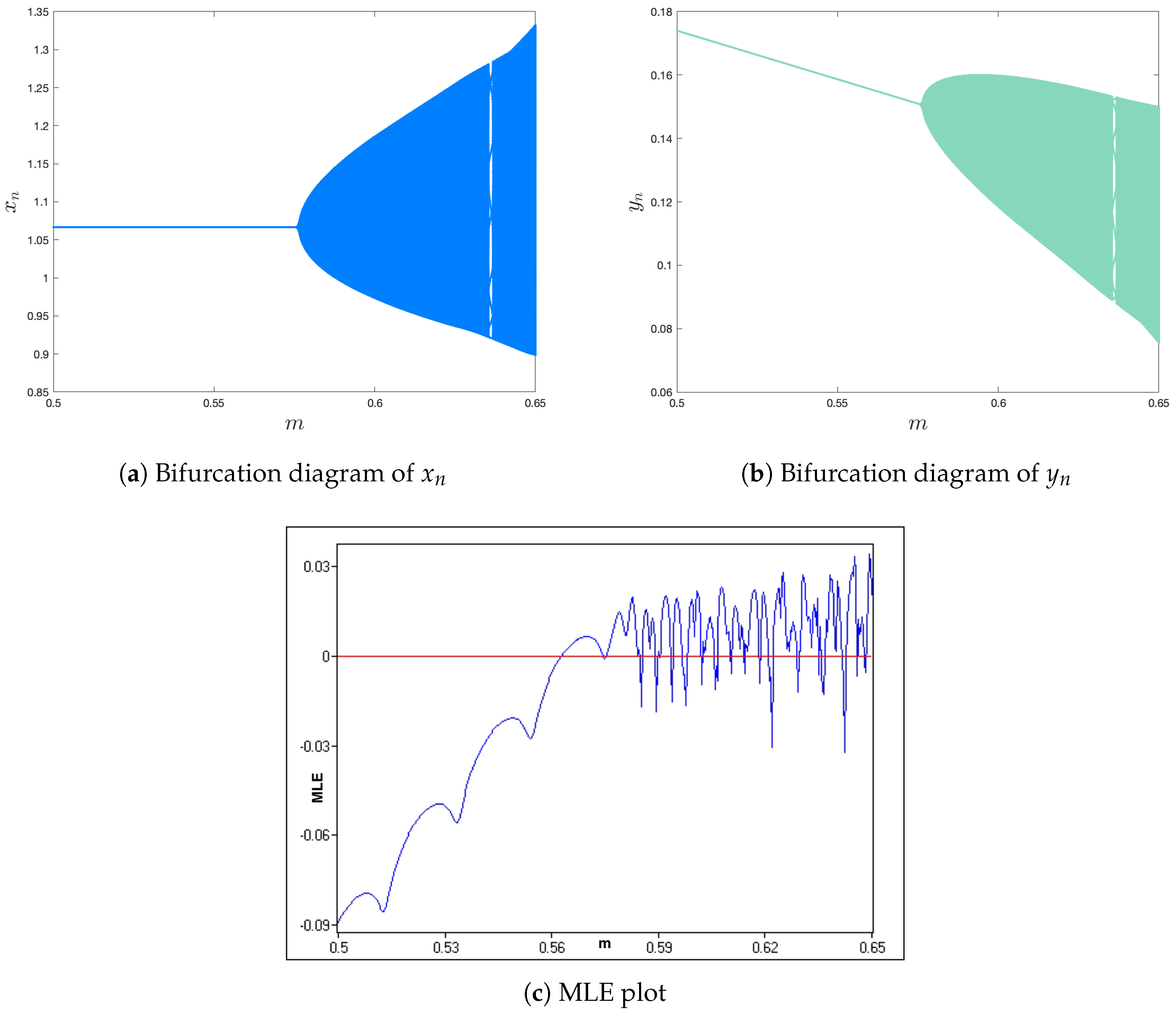
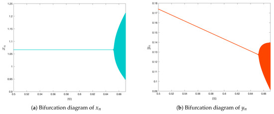
To better understand this process, we plot the bifurcation graphs for the prey and predator populations $x_n$ and $y_n$ as m varies over the range $[0.50,0.65]$; see Figure 2a,b. The values for the initial values are taken as $x_0=1.05$ and $y_0=0.15$. From these graphs, we can see that $E_3$ remains stable for $m<0.576431$, but as soon as m passes this value, the fixed point becomes unstable. This instability gives rise to quasi-periodic cycles, which indicate the presence of a stable closed invariant curve. This is also evident from the graph of maximum Lyapunov exponent (MLE), which is shown in Figure 2c and crosses zero at the bifurcation point. Biologically speaking, this means that there is a transition from a stable coexistence to non-periodic oscillations for prey and predator populations. These quasi-periodic cycles are important in biological contexts because they indicate real-world oscillations that do not converge to a steady-state or periodic solution.

Figure 2. Bifurcation diagrams and the MLE of (4) as the parameter m varies in $[0.50,0.65]$. The diagrams illustrate the transition from stable equilibrium to quasiperiodic behavior via NS bifurcation. Other parameters are fixed at $r=3.1,a=0.1,k=1.5,q=2.5,p=0.75,d=0.8,\mu =1.5$, with initial conditions $x_0=1.05$, $y_0=0.15$.

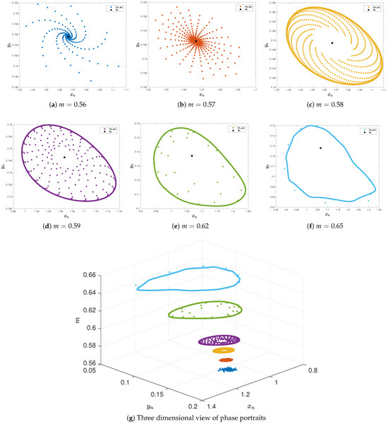
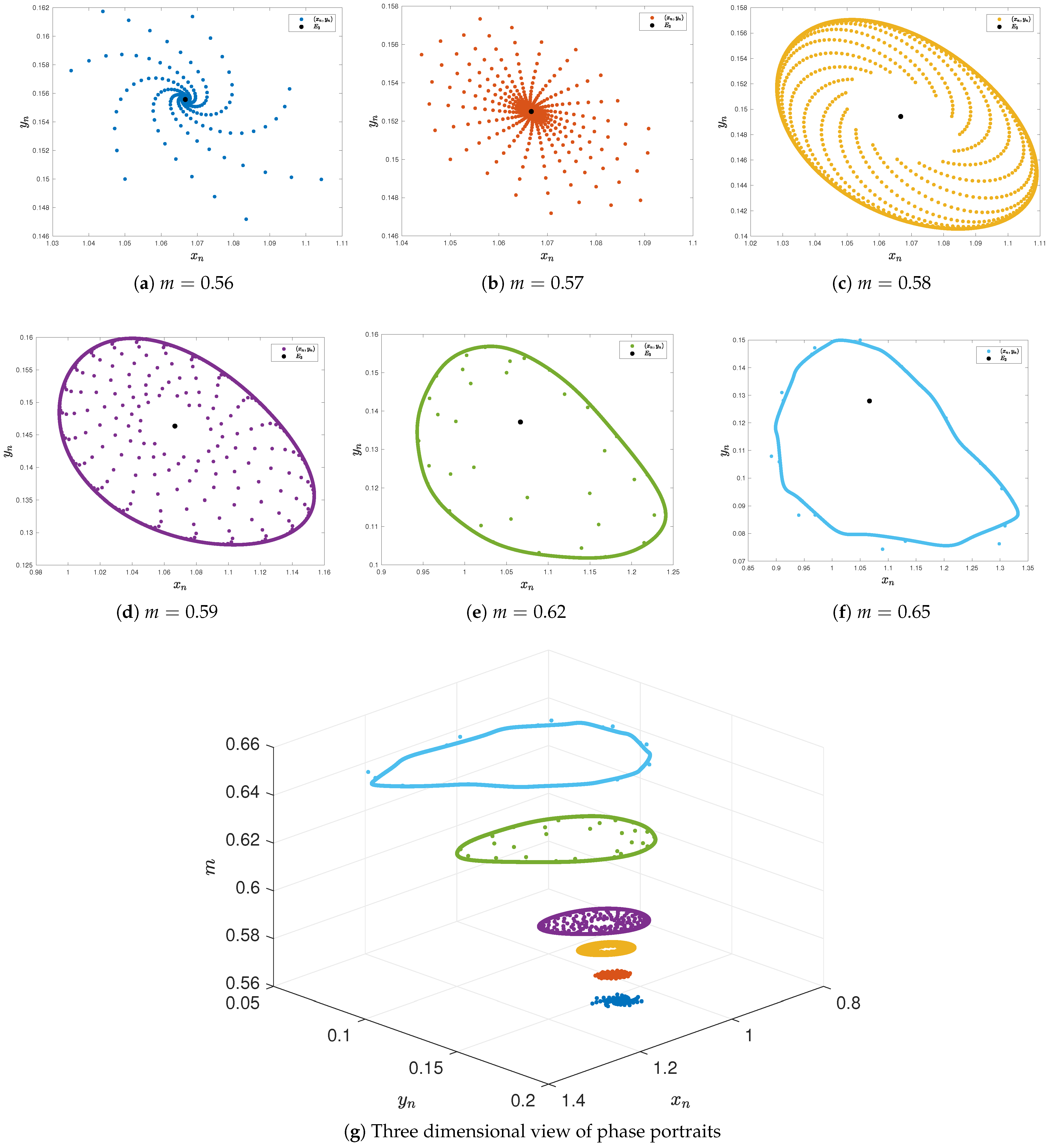
Phase plots of (4) for a few values of m are presented in Figure 3, illustrating the dynamic transition process related to the NS bifurcation. For smaller values of m, such as $m=0.56$ and $m=0.57$ (Figure 3a,b), the trajectories approach the interior fixed point $E_3$, which is locally stable. As m approaches the bifurcation value $m_{NS}\approx 0.576431$, the system’s behavior undergoes a significant change. For $m=0.58$ (Figure 3c), the system undergoes an NS bifurcation, and a closed invariant curve appears, representing the onset of quasi-periodic motion. For $m>m_{NS}$ (Figure 3c–f), $E_3$ loses stability, and the orbits tend to a closed stable limit cycle, representing the NS bifurcation and population oscillations. Figure 3g is the 3D plot for six values of m in Figure 3a–f, showing that the radius of the closed invariant curve increases with the increase in m, further confirming the qualitative change in the system’s behavior with the increase in m.

Figure 3. Phase portraits of (4) for different values of m, illustrating the transition from stable equilibrium to quasiperiodic oscillations. Other parameters are fixed at $r=3.1,a=0.1,k=1.5,q=2.5,p=0.75,d=0.8,\mu =1.5$, with initial conditions $x_0=1.05$, $y_0=0.15$.

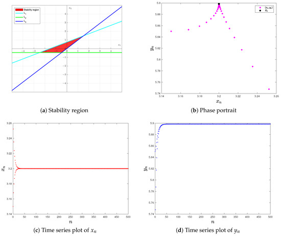
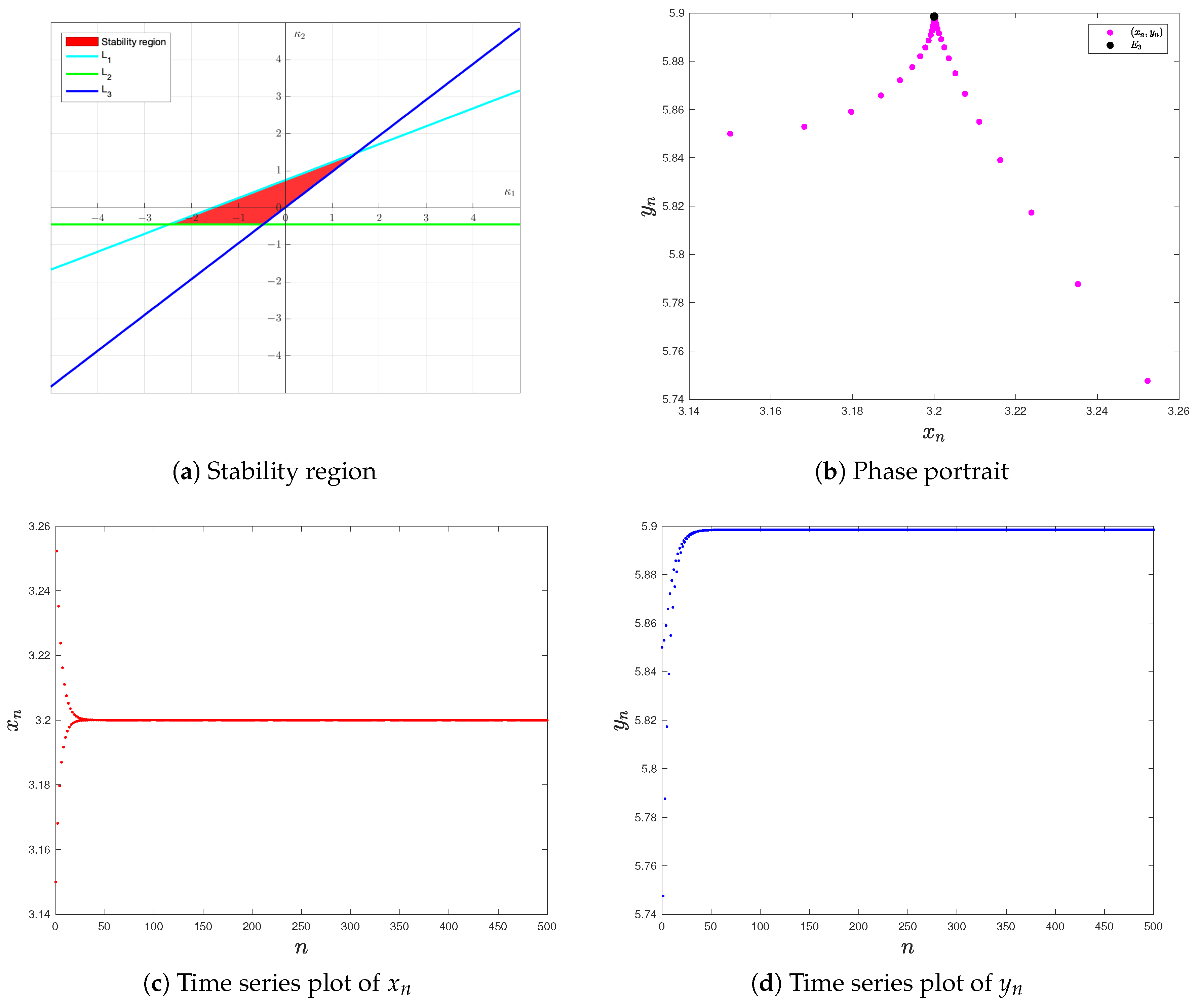
As uncontrolled dynamics above the NS threshold may cause unpredictable fluctuations in the ecosystem, it is necessary to analyze whether control mechanisms can stabilize the system. We analyze the applicability of the feedback control technique to stabilize the system. We consider the parameter values $r=3.1,a=0.1,k=1.5,q=2.5,p=0.75,d=0.8$, and $\mu =1.5$, and choose $m=0.60$, for which the original model (4) goes through an NS bifurcation and $E_3$ is unstable.

For the controlled model (31), we obtain

$$\begin{array}{cc}\hfill L_1:& {\kappa }_2=-0.3663+6.20347{\kappa }_1,\hfill \\ \hfill L_2:& {\kappa }_2=-4,\hfill \\ \hfill L_3:& {\kappa }_2=-21.5465+12.4069{\kappa }_1.\hfill \end{array}$$

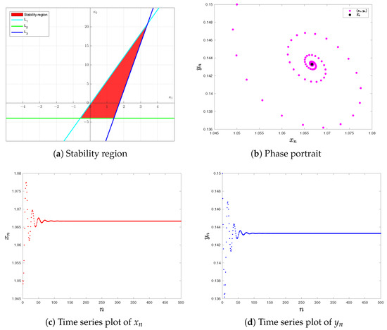
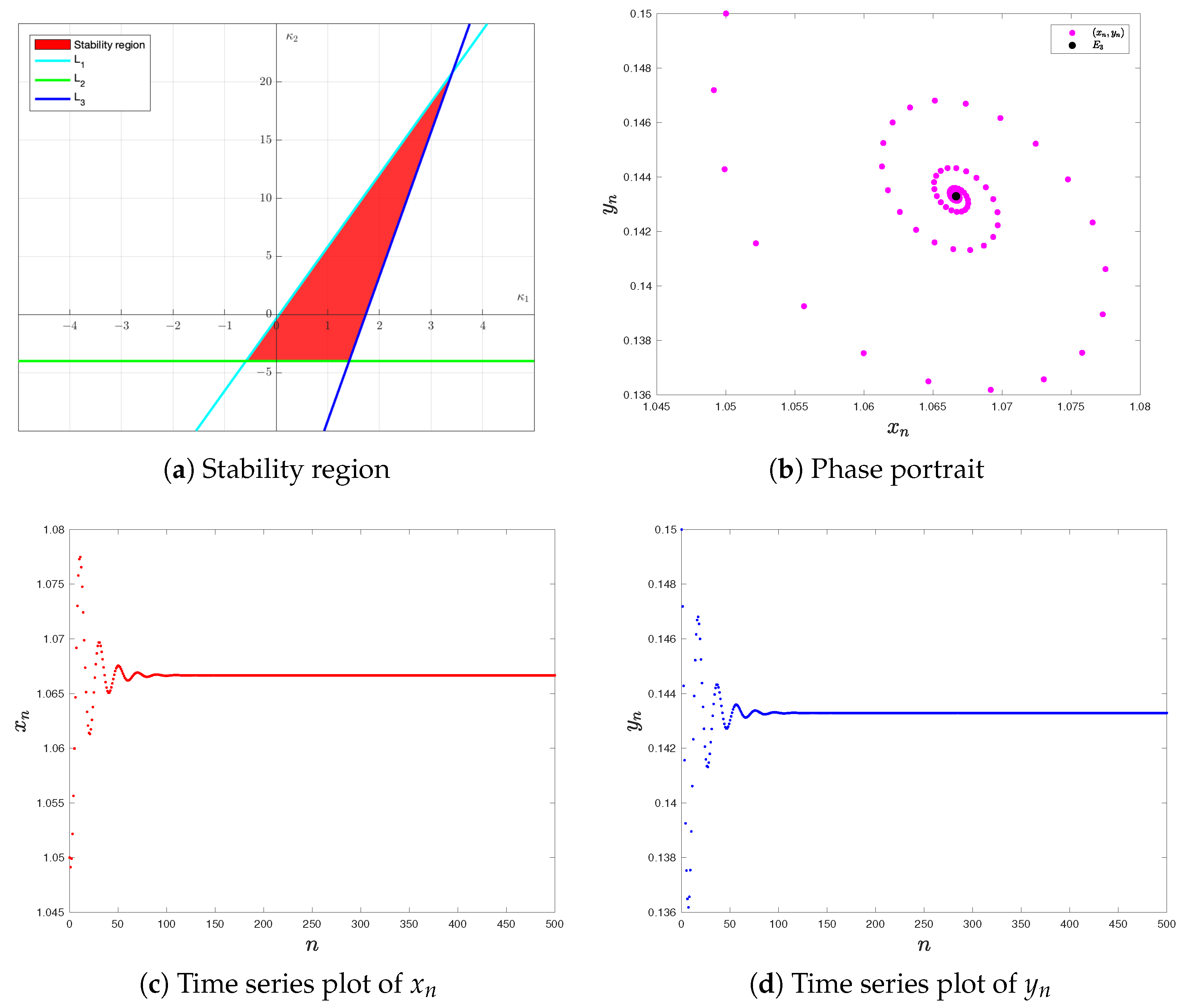
The stability region is depicted in Figure 4a, with boundaries defined by lines $L_1$, $L_2$, and $L_3$. We consider the controlled system with feedback gains ${\kappa }_1=-0.37$ and ${\kappa }_2=-3.39$ which introduce a stabilizing negative feedback mechanism that counteracts deviations of the state variables from their equilibrium levels. The time series of $x_n$ and $y_n$ are presented in Figure 4c and Figure 4d, respectively, and the phase portrait is given in Figure 4b. These figures clearly show that the feedback control approach is successful in preventing the NS bifurcation and stabilizing the system by suppressing oscillations and promoting convergence toward the steady state. From the ecological perspective, the use of feedback control can simulate the impact of external influences, such as controlled harvesting, environmental management, or population control, where negative feedback reflects density-dependent regulatory effects, such as increased harvesting or environmental resistance at higher population levels, that assist in keeping the ecosystem close to a stable equilibrium state.

Figure 4. Stability region in the $({\kappa }_1,{\kappa }_2)$-plane, phase portrait, and time series plots of the controlled system (31), demonstrating stabilization of the dynamics around the equilibrium under state feedback control. The parameters are $r=3.1,a=0.1,k=1.5,q=2.5,p=0.75,d=0.8,\mu =1.5,m=0.60$, with feedback gains ${\kappa }_1=-0.37$, ${\kappa }_2=-3.39$, and initial conditions $x_0=1.05$, $y_0=0.15$.

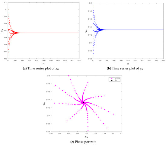
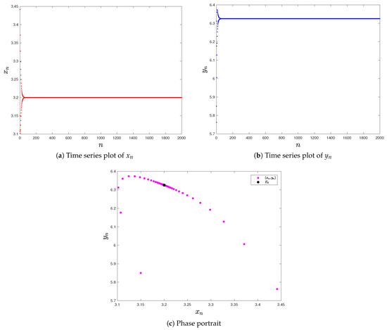
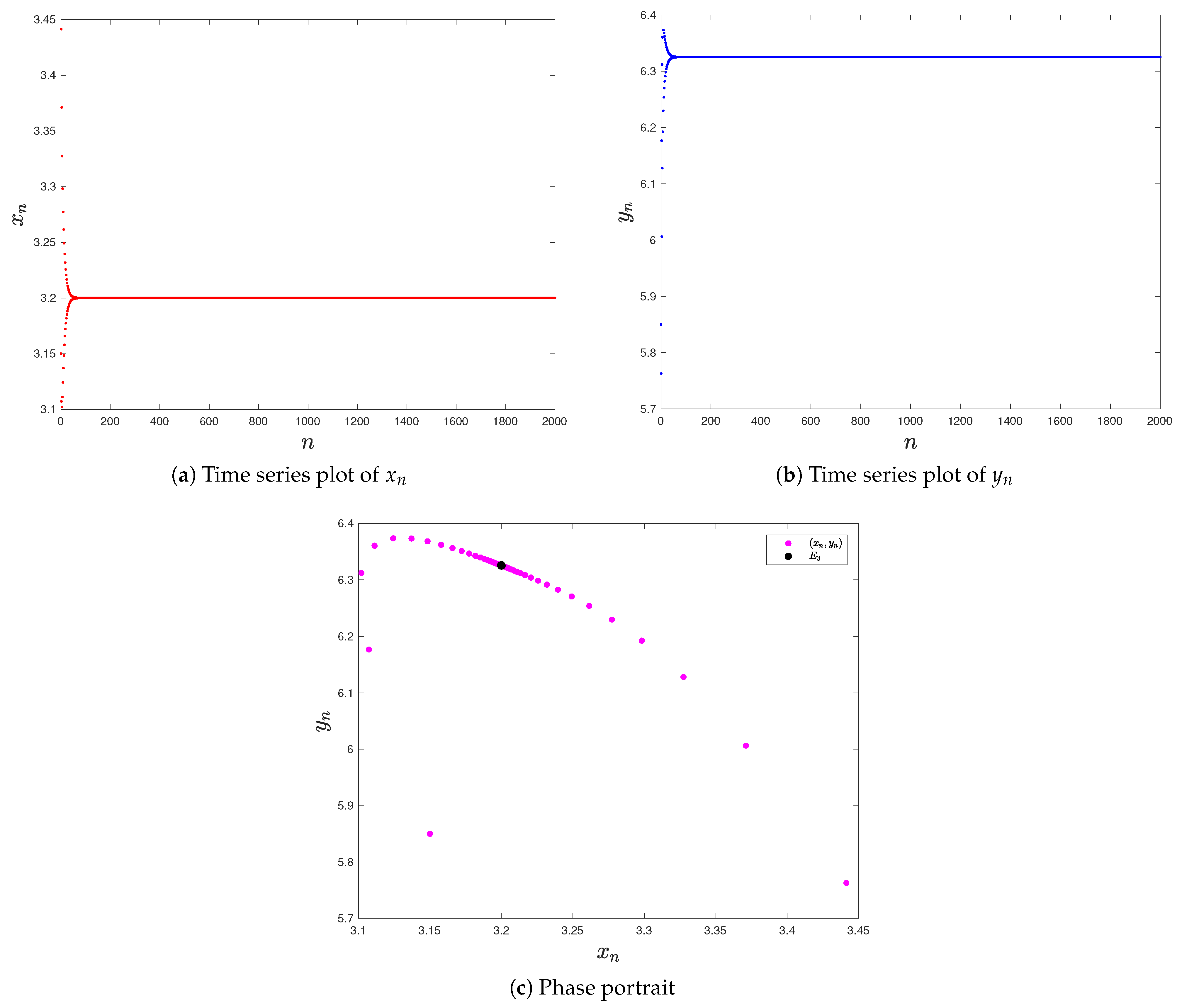
We now examine the effectiveness of the hybrid control method. We fix $\rho =0.85$ and use the parameter values $r=3.1,a=0.1,k=1.5,q=2.5,p=0.75,d=0.8$, and $\mu =1.5$. We consider $m=0.6$, for which the original system (4) becomes unstable due to the occurrence of NS bifurcation. However, under the same set of parameter values, the controlled system exhibits stable behavior, as illustrated by the time series and phase portraits shown in Figure 5.

Figure 5. Time series plots of $x_n$ and $y_n$ and the corresponding phase portrait of the hybrid controlled system (39), illustrating stabilization of the dynamics toward the equilibrium under the control parameter $\rho =0.85$. The parameters are $m=0.6,r=3.1,a=0.1,k=1.5,q=2.5,p=0.75,d=0.8,\mu =1.5$, with initial conditions $x_0=1.05$, $y_0=0.15$.

5.2. PD Bifurcation Analysis and Chaos Control

We investigate the occurrence of a PD bifurcation by varying the parameter m, while fixing the remaining parameters as $r=0.9,a=0.15,k=4.5,q=0.1,p=0.25,d=0.8$, and $\mu =1.4$. For this parameter set, the system undergoes a PD bifurcation at $m=m_{PD}\approx -4.363315$. The corresponding positive fixed point is $E_3\approx (3.2,5.87004)$, with eigenvalues ${\theta }_1=-1$ and ${\theta }_2=0.539789$ of the Jacobian matrix $J\left(E_3\right)$. These eigenvalues satisfy the condition for PD bifurcation, confirming its presence at $m\approx -4.363315$.

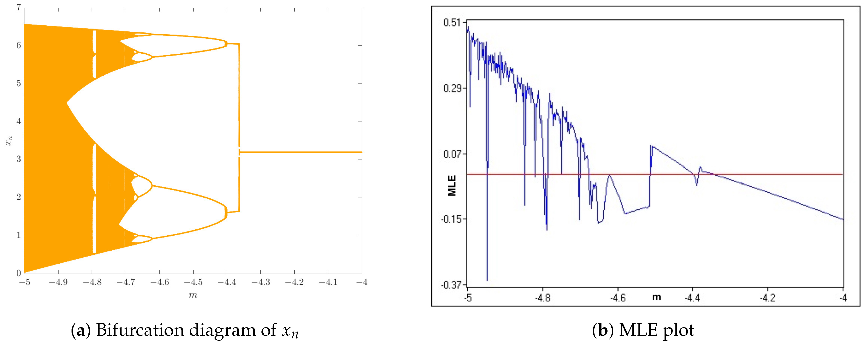
To demonstrate this change, we display the bifurcation diagram of $x_n$ for the range of m from $-5$ to $-4$ in Figure 6a, with the initial values $x_0=3.15$ and $y_0=5.85$. This bifurcation diagram reveals that the fixed point $E_3$ is stable for $m>-4.363315$, but becomes unstable and undergoes a PD bifurcation as m passes below the critical value. The MLE plot corresponding to this bifurcation is shown in Figure 6b, further confirming this bifurcation process. It is important to note that the presence of positive values in the MLE plot confirms the onset of chaotic behavior in the model for specific values of m. The bifurcation diagram and the positive values of the MLE strongly suggest the presence of chaotic behavior for values of m below the bifurcation point. Ecologically speaking, such chaotic behavior could result in unpredictable population levels, further increasing the chances of extinction for one or both species because of the large oscillations.

Figure 6. Bifurcation diagram of $x_n$ and the corresponding MLE for system (4) as m varies in $[-5,-4]$, illustrating the transition from stable behavior to periodic and chaotic dynamics. Positive MLE values indicate chaos. The parameters are fixed at $r=0.9,a=0.15,k=4.5,q=0.1,p=0.25,d=0.8,\mu =1.4$, with initial conditions $x_0=3.15$, $y_0=5.85$.

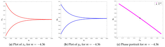
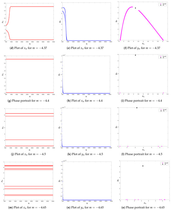
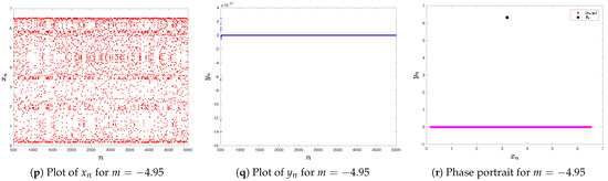
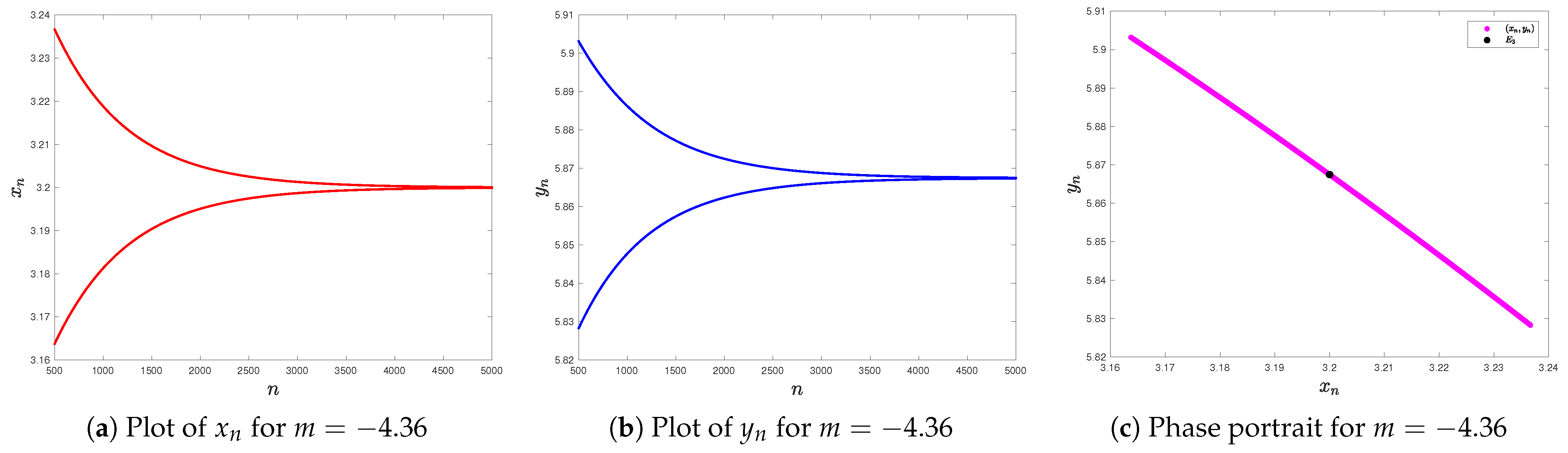
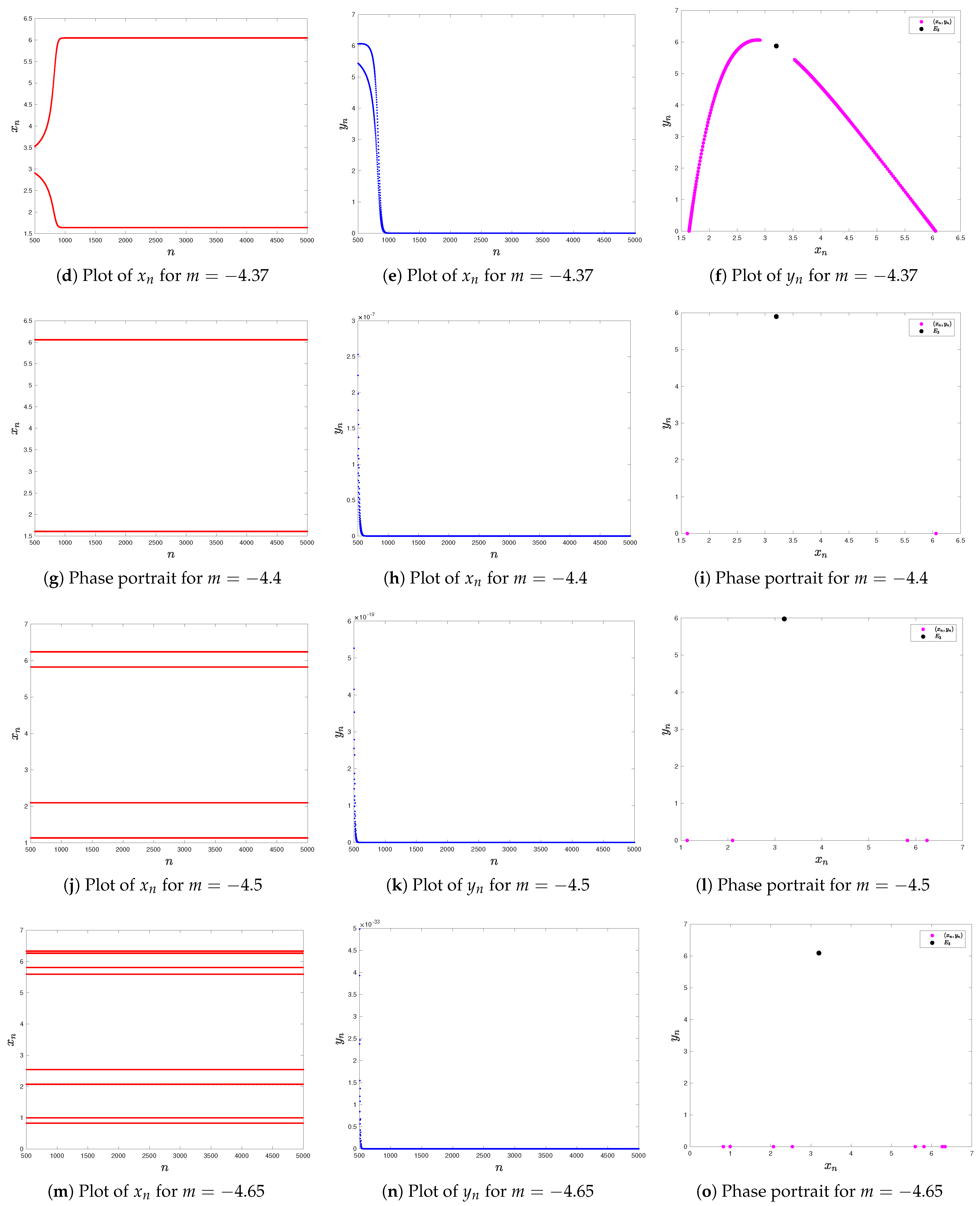
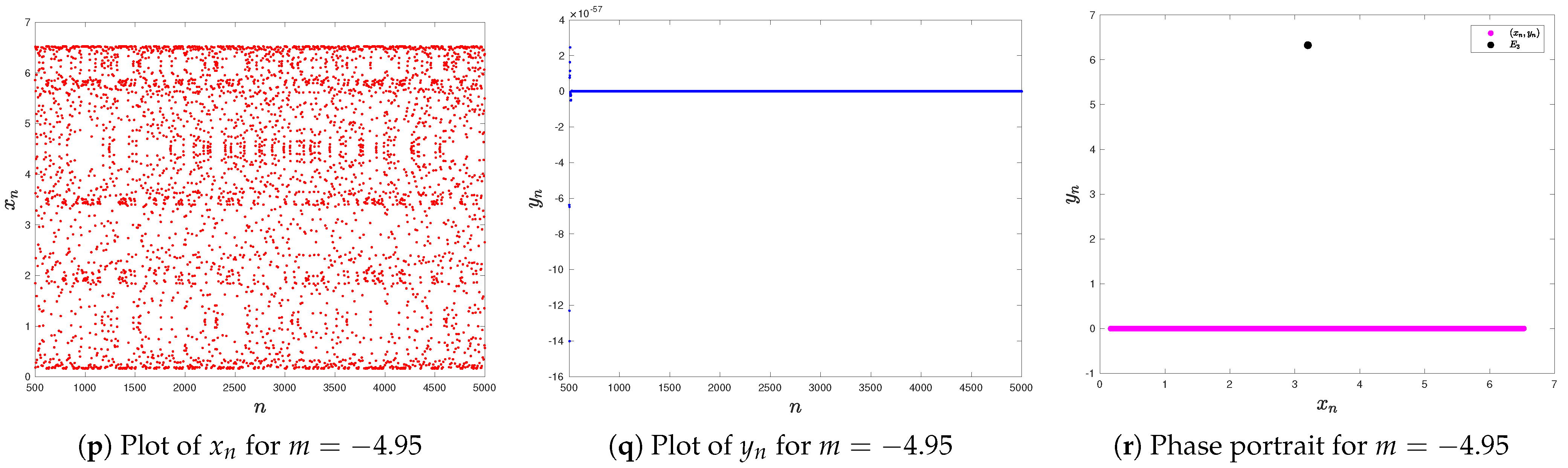
Figure 7 show time series and phase portraits for different values of the parameter m. At first, the positive fixed point is a sink, as shown in Figure 7a–c. However, when the value of the parameter m exceeds the critical value of $m_{PD}\approx -4.363315$, the fixed point loses stability because of a PD bifurcation. This is clear from Figure 7d–f, where the system undergoes a transition from a stable fixed point to a periodic solution. In particular, from Figure 7d–i, the system undergoes a transition to a period-2 orbit, from Figure 7j–l, the system undergoes a transition to a period-4 orbit, and from Figure 7m–o, the system undergoes a transition to a period-8 orbit. The series of PD bifurcations finally leads to chaotic behavior.

Figure 7. Time series plots and phase portraits of model (4) for parameter values $r=0.9,a=0.15,k=4.5,q=0.1,p=0.25,d=0.8,\mu =1.4$ and initial conditions $x_0=3.15,y_0=5.85$, (a–c) $m=-4.36$, (d–f) $m=-4.37$, (g–i) $m=-4.4$, (j–l) $m=-4.5$, (m–o) $m=-4.65$, (p–r) $m=-4.95$.

The PD bifurcation suggests that there is a critical point beyond which the predator–prey interaction dynamics change from stable coexistence to oscillations with periods that double. This could be an indication of real-world ecological processes, such as population cycles caused by environmental stress or overexploitation.

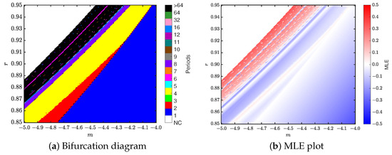
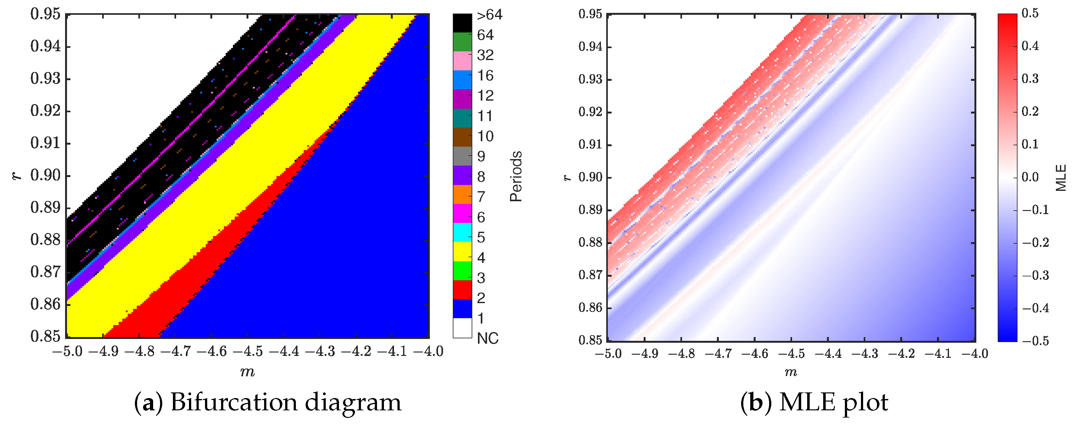
Next, we perform two-parameter bifurcation analysis. Fixing $a=0.15,k=4.5,q=0.1,p=0.25,d=0.8,\mu =1.4$, we vary $m\in [-5,-4]$ and $r\in [0.85,0.95]$. Figure 8a presents a two dimensional bifurcation diagram in the $(m,r)$-plane where different colors are showing different periodic regions. Figure 8b presents the corresponding two-dimensional MLE plot in the $(m,r)$-plane.

Figure 8. Two-dimensional bifurcation diagram and MLE plot of (4) varying $m\in [-5,-4]$ and $r\in [0.85,0.95]$. Fixed parameter values are $a=0.15,k=4.5,q=0.1,p=0.25,d=0.8,\mu =1.4$ and initial values are $x_0=3.15,y_0=5.85$.

Next, we consider $r=0.9,a=0.15,k=4.5,q=0.1,p=0.25,d=0.8,\mu =1.4$, and choose $m=-4.4$, for which (4) goes through a PD bifurcation and $E_3$ becomes unstable. Under these settings, we analyze the controlled system (31), for which the lines of marginal stability in the $({\kappa }_1,{\kappa }_2)$-plane are given by:

$$\begin{array}{cc}\hfill L_1:& {\kappa }_2=0.750284+0.484384{\kappa }_1,\hfill \\ \hfill L_2:& {\kappa }_2=-0.448,\hfill \\ \hfill L_3:& {\kappa }_2=0.011032+0.968768{\kappa }_1.\hfill \end{array}$$

The stability region of the controlled system (31) is shown in Figure 9a, and it is enclosed by the lines $L_1$, $L_2$, and $L_3$. To assess the efficiency of the control method, we choose the feedback control gains ${\kappa }_1=-0.52$ and ${\kappa }_2=-0.33$. The dynamics of the system with these feedback gains are shown in Figure 9, and the time series of $x_n$, $y_n$, and the corresponding phase portrait are shown in Figure 9c, Figure 9d, and Figure 9b, respectively. These results show that the feedback control method is successful in suppressing the effects of the PD bifurcation and the chaotic behavior in the system.

Figure 9. Stability region in the $({\kappa }_1,{\kappa }_2)$-plane, phase portrait, and time series plots of system (31), illustrating stabilization of the dynamics under state feedback control. The parameters are $r=0.9,a=0.15,k=4.5,q=0.1,p=0.25,d=0.8,\mu =1.4,m=-4.4$, with control gains ${\kappa }_1=-0.52$, ${\kappa }_2=-0.33$, and initial conditions $x_0=3.15$, $y_0=5.85$.

We now examine the effectiveness of the hybrid control method. The parameter $\rho$ is fixed at $0.85$, and the remaining parameters are chosen as $r=0.9$, $a=0.15$, $k=4.5$, $q=0.1$, $p=0.25$, $d=0.8$, and $\mu =1.4$. We take $m=-4.95$, for which the original system (4) exhibits chaotic behavior. However, for the same set of parameter values, the controlled system becomes stable, as demonstrated by the time series and phase portraits presented in Figure 10. This confirms the effectiveness of the hybrid control method in suppressing chaos.

Figure 10. Time series plots and phase portrait of (39) by setting $\rho =0.85,m=-4.95,r=0.9,a=0.15,k=4.5,q=0.1,p=0.25,d=0.8,\mu =1.4$ and initial conditions are $x_0=3.15,y_0=5.85$.

5.3. Comparison of Dynamics in Fractional-Order and Integer-Order Models

To emphasize the effect of fractional-order dynamics on system behavior, we compare discretized fractional-order model (4) with its integer-order version by setting $\alpha =1$. We set the parameters to $r=0.9,a=0.15,k=4.5,q=0.1,p=0.25,d=0.8,h=1$. The bifurcation plots for both $x_n$ and $y_n$ are presented in Figure 11. It is noted that the stability region in the integer-order model is larger than that of the fractional-order model. In the integer-order model, the bifurcation threshold value of m is higher, and the system is stable for a larger range of parameters. However, a fractional-order system is more complex, with earlier bifurcations and more complex oscillations. This verifies that the memory effect in the fractional-order model increases the complexity of the system with respect to parameter variations.

Figure 11. Bifurcation diagrams of model (4) varying m. Fixed values are $r=3.1,a=0.1,k=1.5,q=2.5,p=0.75,d=0.8,\alpha =1,h=1$ and initial conditions are $x_0=1.05,y_0=0.15$.

From a biological perspective, this difference indicates that memory effects, together with the double Allee effect, significantly influence the onset of complex dynamics. While the integer-order model predicts a wider region of stable coexistence, the fractional-order model shows that past population states can trigger earlier transitions to oscillatory and quasiperiodic behavior. In particular, the double Allee effect introduces critical thresholds at low prey densities, while memory effects modify how the system responds to these thresholds over time. As a result, their combined influence leads to richer and more sensitive dynamics, including earlier bifurcations and more persistent oscillations compared to the classical model.

5.4. Sensitivity Analysis of Model Parameters

Sensitivity analysis is an important tool in mathematical modeling that is used to examine how changes in model parameters influence the behavior of a system. It plays a significant role in many fields, including ecology, economics, and engineering, where system dynamics are governed by multiple interacting parameters. By performing sensitivity analysis, one can determine which parameters have a strong impact on the system and which have only a minor influence.

To measure this effect quantitatively, a sensitivity index is introduced. For a given parameter p, the sensitivity index is defined as

$$S_p={\displaystyle \frac{\partial \overline{x}}{\partial p}}·{\displaystyle \frac{p}{\overline{x}}},$$

where $\overline{x}$ represents an equilibrium value or another key output of the model. This index provides useful information about both the direction and magnitude of the parameter’s influence. A positive value of $S_p$ indicates that an increase in p leads to an increase in $\overline{x}$, whereas a negative value implies that $\overline{x}$ decreases as p increases. If the sensitivity index is close to zero, it means that the corresponding parameter has only a weak effect on the system output.

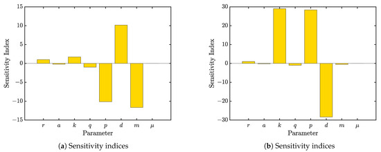
Figure 12 shows the sensitivity indices of the predator equilibrium component for two different parameter sets, where the bars indicate both the magnitude and direction of the influence of each parameter.

Figure 12. Sensitivity indices of the predator equilibrium component for two different parameter sets: (a) $r=2.2,a=1,k=6,q=0.3,p=0.5,d=1.9,m=3.5,\mu =0.6$; (b) $r=2,a=0.8,k=6,q=0.35,p=0.5,d=2.9,m=2,\mu =0.6$.

In both panels, the parameters r and q exhibit consistent behavior: r has a positive effect, implying that increasing the prey growth rate enhances the predator equilibrium, while q has a negative effect, indicating that stronger predation pressure reduces the predator population. The parameters k, m, p, and d display relatively large sensitivity magnitudes, showing that the predator equilibrium is highly sensitive to their variations. In particular, d has a strong negative impact, whereas k and p contribute positively to the predator density. In contrast, the parameter a has only a minor influence, and the parameter $\mu$ has no effect, as reflected by its zero sensitivity index.

For the prey component, the equilibrium $\overline{x}={\displaystyle \frac{d}{p}}$ depends only on d and p. Accordingly, $S_d\left(\overline{x}\right)=1$ and $S_p\left(\overline{x}\right)=-1$, while all other sensitivity indices are zero. This implies that an increase in predator mortality d raises the prey equilibrium, whereas an increase in conversion efficiency p reduces it. Thus, the prey equilibrium is solely governed by the balance between d and p, with no contribution from the remaining parameters.

6. Conclusions

In this work, we have proposed and investigated a discrete-time fractional predator–prey system with a double Allee effect, which offers a model that takes into account memory-dependent behavior and survival conditions at low densities. By employing the piecewise constant argument approach, the proposed model retains the essential properties of the original fractional system and, at the same time, is tractable analytically. We have shown the existence and local stability of all equilibria and have derived explicit conditions for NS and PD bifurcations, which determine the onset of oscillations and complex dynamics. The results obtained show that the combination of fractional memory and the double Allee effect leads to a substantial modification of the stability structure of the system, where the Allee effect can be either stabilizing or destabilizing for population dynamics depending on the choice of parameters. Numerical simulations verify the results obtained by the theory and demonstrate transitions from stable equilibria to periodic, quasi-periodic, and chaotic behavior. In addition, the use of feedback and hybrid control methods demonstrates their effectiveness in eliminating chaos and stabilizing unstable behavior. This study emphasizes the importance of the inclusion of both memory effects and multiple Allee thresholds in ecological modeling and presents a mathematically tractable and dynamically rich framework for understanding and controlling complex population dynamics.

References

- Lotka, A.J. Elements of Physical Biology. Nature 1925, 116, 461. [Google Scholar] [CrossRef] [Scilit]
- Volterra, V. Fluctuations in the Abundance of a Species considered Mathematically. Nature 1926, 118, 558–560. [Google Scholar] [CrossRef] [Scilit]
- Ahmed, R.; Khan, A.Q.; Amer, M.; Faizan, A.; Ahmed, I. Complex Dynamics of a Discretized Predator–Prey System with Prey Refuge Using a Piecewise Constant Argument Method. Int. J. Bifurc. Chaos 2024, 34, 2450120. [Google Scholar] [CrossRef] [Scilit]
- Din, Q.; Jameel, K.; Shabbir, M.S. Discrete-Time Predator–Prey System Incorporating Fear Effect: Stability, Bifurcation, and Chaos Control. Qual. Theory Dyn. Syst. 2024, 23, 285. [Google Scholar] [CrossRef] [Scilit]
- Alsubhi, M.; Ahmed, R.; Alraddadi, I.; Alsharif, F.; Imran, M. Stability and bifurcation analysis of a discrete-time plant-herbivore model with harvesting effect. AIMS Math. 2024, 9, 20014–20042. [Google Scholar] [CrossRef] [Scilit]
- Shabbir, M.S.; Din, Q. Understanding Cannibalism Dynamics in Predator–Prey Interactions: Bifurcations and Chaos Control Strategies. Qual. Theory Dyn. Syst. 2024, 23, 53. [Google Scholar] [CrossRef] [Scilit]
- Javaid, Y.; Jawad, S.; Ahmed, R.; Ali, A.H.; Rashwani, B. Dynamic complexity of a discretized predator-prey system with Allee effect and herd behaviour. Appl. Math. Sci. Eng. 2024, 32, 2420953. [Google Scholar] [CrossRef] [Scilit]
- Allee, W.C. Animal Aggregations, a Study in General Sociology; The University of Chicago Press: Chicago, IL, USA, 1931. [Google Scholar] [CrossRef] [Scilit]
- AlSharawi, Z.; Pal, S.; Pal, N.; Chattopadhyay, J. A discrete-time model with non-monotonic functional response and strong Allee effect in prey. J. Differ. Equ. Appl. 2020, 26, 404–431. [Google Scholar] [CrossRef] [Scilit]
- Zhang, L.; Zou, L. Bifurcations and Control in a Discrete Predator–Prey Model with Strong Allee Effect. Int. J. Bifurc. Chaos 2018, 28, 1850062. [Google Scholar] [CrossRef] [Scilit]
- Ma, Y.; Zhao, M.; Du, Y. Impact of the strong Allee effect in a predator-prey model. AIMS Math. 2022, 7, 16296–16314. [Google Scholar] [CrossRef] [Scilit]
- Zhao, L.; Shen, J. Relaxation oscillations in a slow–fast predator–prey model with weak Allee effect and Holling-IV functional response. Commun. Nonlinear Sci. Numer. Simul. 2022, 112, 106517. [Google Scholar] [CrossRef] [Scilit]
- Dong, Y.; Liu, H.; Wei, Y.; Zhang, Q.; Ma, G. Stability and Hopf Bifurcation Analysis of a Predator-Prey Model with Weak Allee Effect Delay and Competition Delay. Mathematics 2024, 12, 2853. [Google Scholar] [CrossRef] [Scilit]
- Zhang, L.; Wang, T. Qualitative properties, bifurcations and chaos of a discrete predator-prey system with weak Allee effect on the predator. Chaos Solitons Fractals 2023, 175, 113995. [Google Scholar] [CrossRef] [Scilit]
- Wang, F.; Yang, R.; Zhang, X. Turing patterns in a predator-prey model with double Allee effect. Math. Comput. Simul. 2024, 220, 170–191. [Google Scholar] [CrossRef] [Scilit]
- Tiwari, B.; Raw, S.N. Dynamics of Leslie-Gower model with double Allee effect on prey and mutual interference among predators. Nonlinear Dyn. 2021, 103, 1229–1257. [Google Scholar] [CrossRef] [Scilit]
- Pal, P.J.; Saha, T. Qualitative analysis of a predator-prey system with double Allee effect in prey. Chaos Solitons Fractals 2015, 73, 36–63. [Google Scholar] [CrossRef] [Scilit]
- Sen, D.; Ghorai, S.; Banerjee, M.; Morozov, A. Bifurcation analysis of the predator–prey model with the Allee effect in the predator. J. Math. Biol. 2022, 84, 7. [Google Scholar] [CrossRef] [Scilit] [PubMed]
- Zeng, Y.; Yu, P. Complex Dynamics of Predator-Prey Systems with Allee Effect. Int. J. Bifurc. Chaos 2022, 32, 2250203. [Google Scholar] [CrossRef] [Scilit]
- Song, N. Bifurcation and Chaos of a Nonlinear Discrete-Time Predator-Prey Model Involving the Nonlinear Allee Effect. Discret. Dyn. Nat. Soc. 2023, 2023, 5475999. [Google Scholar] [CrossRef] [Scilit]
- González-Olivares, E.; González-Yaez, B.; Lorca, J.M.; Rojas-Palma, A.; Flores, J.D. Consequences of double Allee effect on the number of limit cycles in a predator–prey model. Comput. Math. Appl. 2011, 62, 3449–3463. [Google Scholar] [CrossRef] [Scilit]
- Xia, S.; Li, X. Complicate dynamics of a discrete predator-prey model with double Allee effect. Math. Model. Control 2022, 2, 282–295. [Google Scholar] [CrossRef] [Scilit]
- Magin, R.L. Fractional calculus models of complex dynamics in biological tissues. Comput. Math. Appl. 2010, 59, 1586–1593. [Google Scholar] [CrossRef] [Scilit]
- Almeida, R.; Bastos, N.R.O.; Monteiro, M.T.T. Modeling some real phenomena by fractional differential equations. Math. Methods Appl. Sci. 2016, 39, 4846–4855. [Google Scholar] [CrossRef] [Scilit]
- Li, H.L.; Zhang, L.; Hu, C.; Jiang, Y.L.; Teng, Z. Dynamical analysis of a fractional-order predator-prey model incorporating a prey refuge. J. Appl. Math. Comput. 2017, 54, 435–449. [Google Scholar] [CrossRef] [Scilit]
- Tang, B. Dynamics for a fractional-order predator-prey model with group defense. Sci. Rep. 2020, 10, 4906. [Google Scholar] [CrossRef] [Scilit] [PubMed]
- Singh, A.; Elsadany, A.A.; Elsonbaty, A. Complex dynamics of a discrete fractional-order Leslie-Gower predator-prey model. Math. Methods Appl. Sci. 2019, 42, 3992–4007. [Google Scholar] [CrossRef] [Scilit]
- Sarkar, K.; Mondal, B. Dynamic analysis of a fractional-order predator–prey model with harvesting. Int. J. Dyn. Control 2023, 11, 1518–1531. [Google Scholar] [CrossRef] [Scilit]
- Mondal, C.; Mondal, R.; Kesh, D.; Mukherjee, D. Dynamics of predator-prey system with the consequences of double Allee effect in prey population. J. Biol. Phys. 2025, 51, 5. [Google Scholar] [CrossRef] [Scilit]
- Elsadany, A.A.; Matouk, A.E. Dynamical behaviors of fractional-order Lotka–Volterra predator–prey model and its discretization. J. Appl. Math. Comput. 2015, 49, 269–283. [Google Scholar] [CrossRef] [Scilit]
- Mondal, S.; Biswas, M.; Bairagi, N. Local and global dynamics of a fractional-order predator–prey system with habitat complexity and the corresponding discretized fractional-order system. J. Appl. Math. Comput. 2020, 63, 311–340. [Google Scholar] [CrossRef] [Scilit]
- Uddin, M.J.; Rana, S.M.S.; Işık, S.; Kangalgil, F. On the qualitative study of a discrete fractional order prey–predator model with the effects of harvesting on predator population. Chaos Solitons Fractals 2023, 175, 113932. [Google Scholar] [CrossRef] [Scilit]
- Uddin, M.J.; Podder, C.N. Fractional order prey-predator model incorporating immigration on prey: Complexity analysis and its control. Int. J. Biomath. 2023, 17, 2350051. [Google Scholar] [CrossRef] [Scilit]
- Ara, R.; Rana, S.M.S. Complex Dynamics and Chaos Control of Discrete Prey–Predator Model With Caputo Fractional Derivative. Complexity 2025, 2025, 4415022. [Google Scholar] [CrossRef] [Scilit]
- Matouk, A.E.; Elsadany, A.A. Dynamical analysis, stabilization and discretization of a chaotic fractional-order GLV model. Nonlinear Dyn. 2016, 85, 1597–1612. [Google Scholar] [CrossRef] [Scilit]
- Al-Nassir, S. Dynamic analysis of a harvested fractional-order biological system with its discretization. Chaos Solitons Fractals 2021, 152, 111308. [Google Scholar] [CrossRef] [Scilit]
- Gurcan, F.; Kartal, N.; Kartal, S. Bifurcation and chaos in a fractional-order Cournot duopoly game model on scale-free networks. Int. J. Bifurc. Chaos 2024, 34, 2450103. [Google Scholar] [CrossRef] [Scilit]
- Kartal, N. Multiple Bifurcations and Chaos Control in a Coupled Network of Discrete Fractional Order Predator-Prey System. Iran. J. Sci. 2025, 49, 93–106. [Google Scholar] [CrossRef] [Scilit]
- Luo, A.C.J. Regularity and Complexity in Dynamical Systems; Springer: New York, NY, USA, 2012. [Google Scholar]
- Guckenheimer, J.; Holmes, P. Nonlinear Oscillations, Dynamical Systems, and Bifurcations of Vector Fields; Springer: New York, NY, USA, 1983; Volume 42. [Google Scholar] [CrossRef] [Scilit]
- Wiggins, S.; Golubitsky, M. Introduction to Applied Nonlinear Dynamical Systems and Chaos; Springer: New York, NY, USA, 2003; Volume 2. [Google Scholar] [CrossRef] [Scilit]
- Chen, G.; Dong, X. From Chaos to Order; World Scientific: Singapore, 1998; Volume 24. [Google Scholar] [CrossRef]
- Lei, C.; Han, X.; Wang, W. Bifurcation analysis and chaos control of a discrete-time prey-predator model with fear factor. Math. Biosci. Eng. 2022, 19, 6659–6679. [Google Scholar] [CrossRef] [Scilit]
- Luo, X.S.; Chen, G.; Wang, B.H.; Fang, J.Q. Hybrid control of period-doubling bifurcation and chaos in discrete nonlinear dynamical systems. Chaos Solitons Fractals 2003, 18, 775–783. [Google Scholar] [CrossRef] [Scilit]
Disclaimer/Publisher’s Note: The statements, opinions and data contained in all publications are solely those of the individual author(s) and contributor(s) and not of MDPI and/or the editor(s). MDPI and/or the editor(s) disclaim responsibility for any injury to people or property resulting from any ideas, methods, instructions or products referred to in the content. |
© 2026 by the authors. Licensee MDPI, Basel, Switzerland. This article is an open access article distributed under the terms and conditions of the Creative Commons Attribution (CC BY) license.