


Abstract
While superdeterministic and fractal spacetime models offer compelling alternative perspectives on quantum foundations, the simulation and validation of effective wave dynamics in such non-differentiable, deterministic settings remain computationally and theoretically challenging. To address this, a framework built around the Fractional Nonlinear Klein–Gordon Equation (FNKGE), defined through the spectral fractional Laplacian, was developed. This equation was solved and benchmarked through a comparative study between Physics-Informed Neural Networks (PINNs) with Fourier features and Physics-Informed Graph Neural Networks (PI-GNNs). Additionally, detection patterns were simulated via deterministic agents, and theoretical links between fractal geometry, computational irreducibility, and deviations from statistical independence were formalized. Regarding the computational evaluation, superior accuracy was achieved by the PI-GNNs, yielding a mean relative error of (), alongside faster convergence and a more well-conditioned Hessian spectrum compared to PINNs. Crucially, a continuous power-law decay () was revealed by the spectral analysis of the simulated detection patterns, confirming the emergence of classical optical caustics rather than discrete quantum-interference peaks. Furthermore, a modified dispersion relation that accurately predicts linear instability regimes was derived, and specific boundary artifacts in non-periodic domains were identified. Taken together, the FNKGE is validated by these results as a viable effective model for fractal wave phenomenology and as a robust benchmark for physics-informed learning architectures.
1. Introduction
Quantum mechanics is one of the most empirically successful theories in modern physics, yet its formalism continuously challenges classical notions of realism, locality, and causality [1,2]. Bell test experiments with loophole closures have strengthened the operational conclusion that nature violates Bell inequalities under controlled configurations, ruling out local hidden-variable models under standard assumptions [3,4,5,6].
However, this exclusion applies specifically to the conjunction of local realism and the statistical independence of measurement settings. Consequently, deterministic frameworks remain theoretically viable if the assumption of statistical independence (often termed “free choice”) is relaxed in a structural, non-conspiratorial manner, or if the concept of locality is re-evaluated within a non-smooth geometric substrate [7,8,9,10,11,12].
Aligning with this line of inquiry, we investigate whether a deterministic model posed on a fractal and topologically non-trivial geometric substrate can reproduce effective wave phenomena relevant to quantum-foundational discussions without assuming fundamental indeterminacy from the outset. The emphasis of the present manuscript is deliberately limited: rather than claiming a derivation of quantum mechanics, we study whether multi-scale propagation, non-local dispersion, and structured detection patterns can emerge as effective signatures of deterministic dynamics on a non-smooth background [13,14,15,16,17,18,19,20,21,22,23,24]. In this context, indeterminacy is treated as an epistemological boundary linked to formal incompleteness, algorithmic randomness, and limited predictive compressibility, rather than as a primary ontological feature [25,26,27].
The primary contributions of this work are as follows. First, we formulate a mathematical connection between the measure on the state space and the Hausdorff dimension of the attractor (Lemma 1), suggesting a possible mechanism by which deviations from statistical independence may arise from multifractal structures without explicit fine-tuning, with the fractal measure treated as singularly continuous with respect to the Lebesgue measure. Second, we propose a theoretical link between computational irreducibility and chaotic dynamics by relating the Kolmogorov complexity of trajectories to the metric entropy of the system, thereby motivating how deterministic dynamics may appear effectively unpredictable. Third, we use Fourier spectral analysis of the detection patterns to distinguish between classical optical caustics and interference with discrete fringe frequencies, and we show that the simulated patterns reported here are consistent with the former rather than with genuine quantum interference. Fourth, we evaluate the proposed Fractional Nonlinear Klein–Gordon Equation (FNKGE) through a comparative benchmark of Physics-Informed Neural Networks (PINNs) and Physics-Informed Graph Neural Networks (PI-GNNs). This includes convergence analysis, loss landscape characterization, Hessian spectrum diagnostics, and error quantification against asymptotic reference solutions. Fifth, we analyze the physical limitations of Fast Fourier Transform (FFT) implementations in non-periodic domains and outline a formal roadmap for extending the model to 3+1D frameworks with spinors and gauge fields. Sixth, we present a linear stability analysis of the FNKGE, deriving a modified dispersion relation for plane waves in the fractal substrate to characterize instability regimes. Overall, this article positions these results as evidence for the computational viability of an effective fractal wave model, rather than as a derivation of quantum mechanics from first principles [28,29,30].
This article is organized as follows. Section 2 reviews the foundations of geometric superdeterminism, fractal spacetime modeling, and physics-informed approaches relevant to the proposed effective framework. Section 3 outlines the theoretical postulates and the fractal geometric formalism, including Lemma 1. Section 4 derives the FNKGE with the spectral fractional Laplacian operator. Section 5 presents the linear stability analysis. Section 6 details the computational methodology utilizing PINNs and PI-GNNs. Section 7 reports the simulation results and the spectral analysis. Section 8 provides the numerical validation and error quantification. Section 9 discusses physical interpretation, computational irreducibility, and model limitations. Section 10 synthesizes the findings and future perspectives.
2. State of the Art
2.1. Superdeterminism and the Invariant Set Hypothesis
Superdeterminism posits that the correlation between hidden variables and measurement settings is not conspiratorial, but rather a consequence of the deterministic evolution of the universe from a shared initial condition. ’t Hooft has explored this avenue, suggesting that quantum-like behavior might emerge from an underlying deterministic framework at the Planck scale, potentially modeled via cellular automata [7,8].
A prominent framework within this domain is Tim Palmer’s Invariant Set Theory [9,31]. Palmer proposes that the universe evolves on a fractal attractor in state space. Under this geometric assumption, counterfactual states—those describing hypothetical alternative measurement settings—do not belong to the invariant set and are thus considered physically unrealizable. In this model, the violation of statistical independence arises not from a traditional common cause, but from an atemporal geometric restriction in the space of physical possibilities, bypassing the need for conspiratorial fine-tuning [10]. The taxonomy of theories beyond quantum mechanics proposed by Adlam [11] classifies this approach as a “retrocausal non-fine-tuned” model, where global spacetime constraints influence local events [11].
Figure 1 illustrates this concept: the fractal invariant set in state space (panel a), the discretization of the Bloch sphere with allowed and forbidden states (panel b), and the prediction of Bell inequality violation under fractal correction (panel c).
Figure 1.
Fractal invariant set and violation of statistical independence. (a) Invariant set in state space (Julia-like approximation). (b) Discretized Bloch sphere: allowed states (red) vs. forbidden counterfactuals (gray). (c) CHSH parameter: quantum prediction (blue), fractal correction (red dashed), and classical bound (green).
2.2. Fractal Geometry and Scale Relativity
In the framework of Scale Relativity, Nottale models spacetime as a fractal manifold where physical laws are explicitly dependent on the scale of observation [13,15]. Within this context, Nottale reconstructs a Schrödinger-like equation from fluid mechanics principles in a non-differentiable space, interpreting quantum trajectories as geodesics characterized by a Hausdorff dimension [14,16]. Similarly, Ord [17] showed that a random walk over a fractal geometry can reproduce formal aspects of the Schrödinger equation.
The mathematical treatment of dynamics in such spaces relies heavily on fractional calculus. The fractional Laplacian, , acts as a pseudo-differential operator that captures the non-local nature of anomalous diffusion (Lévy flights) in fractal media [32,33,34,35,36,37,38,39]. Laskin [40,41] expanded the Feynman path integral formalism by substituting Brownian trajectories with Lévy flights, deriving a fractional Schrödinger equation and laying the groundwork for fractional quantum mechanics and fractional thermodynamics [42]. Recent high-precision numerical implementations (e.g., sixth-order split-step methods) have shown the applicability of these equations to model exotic vortex dynamics [28]. As detailed by Lischke et al. [43], this fractional operator is intrinsically non-local, defined via a singular integral (Riesz definition) or a Fourier multiplier.
Figure 2 illustrates the mathematical structures underlying the FNKGE framework. (a) Construction of the Cantor set (): topological incompleteness. (b) Lorenz strange attractor: deterministic chaos in phase space. (c) Sierpinski gasket (): self-similar topology.
Figure 2.
Mathematical structures underlying the FNKGE framework. (a) Construction of the Cantor set (): topological incompleteness, where the solid lines represent the remaining closed intervals at each iteration depth. (b) Lorenz strange attractor: deterministic chaos in phase space, with the color gradient indicating the time evolution of the system’s trajectory. (c) Sierpinski gasket (): self-similar topology.
2.3. The Computational Universe
Computational models of the universe, such as those advanced by Wolfram, propose that physical laws may emerge from iterative computational rules operating on discrete structures like hypergraphs [23,24]. Gorard [44] has investigated how certain relativistic and gravitational features might be recovered within these discrete architectures. A key concept in this approach is computational irreducibility—the principle that the future state of a complex system cannot be predicted by an algorithmic shortcut faster than simulating the system’s evolution step by step. This concept provides a conceptual bridge between deterministic chaos and algorithmic randomness, offering an alternative lens through which to interpret apparent quantum randomness.
2.4. Physics-Informed Deep Learning
PINNs, introduced by Raissi, Perdikaris, and Karniadakis, integrate Partial Differential Equations (PDEs) directly into the neural network’s loss function, ensuring that the training process respects physical constraints [45,46]. Pang et al. [47] extended this methodology to fractional PDEs (fPINNs), showing that the fractional Laplacian can be incorporated spectrally within the PINN architecture [48].
Despite their success, standard PINNs are known to exhibit spectral bias, a tendency to learn low-frequency components significantly faster than high-frequency variations [49]. To address this, techniques such as Fourier Feature Embeddings have been employed to enhance the resolution of high-frequency dynamics [50]. Furthermore, specialized architectures designed for unbounded fractional domains (fs-PINNs) [29] and Transformer-based models (PINNsFormer) [30] have recently broadened the applicability of these algorithms.
For non-Euclidean domains, Graph Neural Networks (GNNs) provide a highly suitable topological framework [51,52]. The recent literature on Physics-Informed GNNs (PI-GNNs) illustrates how the PDE residual can be evaluated and minimized directly on a graph structure, successfully combining the relational inductive bias of GNNs with the rigorous physical regularization characteristic of PINNs [53,54,55].
3. Theoretical Framework and Postulates
The proposed theoretical framework relies on five interrelated postulates that structure the variational, geometric, and probabilistic aspects of the model. These postulates are introduced as components of an exploratory effective description motivated by quantum-foundational questions, not as a completed replacement for standard quantum theory. Their role is to connect an assumed fractal microstructure of spacetime with effective field dynamics and observable statistical signatures within a computationally testable setting.
Postulate 1 (Global Action Principle).
The dynamics of the scalar field over the fractal spacetime substrate are modeled via a global variational principle:
where Ω represents the spacetime domain (which may possess non-trivial topology) and is the Lagrangian density.
Postulate 2 (Fractal Substrate).
The model assumes the underlying spacetime is non-differentiable at fine scales, characterized by a Hausdorff dimension (where d is the topological dimension). This microstructure is formally encoded through the fractional Laplacian operator , where the parameter quantifies the deviation from a smooth geometry [56].
Postulate 3 (Symmetry as Inductive Bias).
The symmetries of the Lagrangian act as constraints that reduce the effective dimensionality of the solution space during the variational optimization (Postulate 1). Following Noether’s theorem, each continuous symmetry induces a conserved current satisfying , which operates computationally as an inductive bias restricting the permissible state space.
Postulate 4
(Spontaneous Symmetry Breaking as Bifurcation).
Within this framework, spontaneous symmetry breaking (SSB) functions as a bifurcation mechanism that selects a specific local minimum (vacuum) within the energy landscape. The selection process is influenced by global boundary conditions and the topological features of the fractal substrate (Figure 3).
Figure 3.
Spontaneous symmetry breaking potential. (a) 1D cut showing the unstable maximum (solid line) at and the parabolic shapes of the degenerate minima . (b) 3D “Mexican hat” potential showing the manifold of degenerate vacua. (c) Dynamical SSB transition: temporal evolution of the field from the unstable vacuum toward a vacuum selected by topology.
Postulate 5 (Fractal Measure and Violation of Statistical Independence).
Let be the complete state space of the modeled system and the fractal attractor governing its evolution. The probability of finding the system in a region is described not by the standard Lebesgue measure , but by a fractal measure supported on :
where is the Hausdorff dimension of the attractor and the sum runs over an ϵ-fine cover. This measure is singularly continuous with respect to . A proposed consequence of this geometric restriction is the violation of statistical independence: let λ be a hidden variable and a a measurement setting. Since both λ and a depend on the global state evolving on , the conditional probability satisfies
This inequality suggests that the choice of a restricts the accessible subset of , thus altering the effective measure over λ. This aligns with the concepts proposed by Palmer [10], wherein the correlation between λ and a emerges from the fractal geometry of the attractor rather than fine-tuning [12,57,58].
The following lemma outlines the mathematical connection between the geometric properties of the attractor and the probabilistic violation of statistical independence within this framework.
Lemma 1 (Fractal Measure Restriction and SI Violation).
Let be a compact fractal attractor in equipped with its natural (Sinai–Ruelle–Bowen) measure , and let be its Hausdorff dimension. Let and be measurable functions representing hidden variables and measurement settings, respectively. Define the sub-attractor for . If the following conditions hold:
- (C1)
- is singularly continuous with respect to the Lebesgue measure , i.e., ;
- (C2)
- The attractor exhibits a non-trivial multifractal structure: there exist distinct points such that the local Hölder exponents satisfy ;
- (C3)
- The map A is not -almost everywhere constant on , and intersects regions of with non-uniform local dimension;
then for -almost every , indicating a violation of statistical independence.
Proof.
The proof proceeds in three steps.
Step 1 (Singular continuity of the restricted measure). Since by (C1), there exists a Borel set such that and . The set S carries all the -mass, and assigns zero probability to any set of positive Lebesgue measures. For any measurable a, the restricted measure is also supported on a subset of with -measure zero, hence .
Step 2 (Non-uniform reweighting under restriction). By (C2), the multifractal spectrum of is non-degenerate. Specifically, the generalized dimensions satisfy for some . This implies that the measure concentrates heterogeneously across .
By (C3), the constraint selects a subset that samples these regions non-uniformly. Let denote the multifractal spectrum. The restricted measure induces an effective spectrum because the intersection preferentially samples specific scaling regions.
Step 3 (Violation of statistical independence). The marginal distribution of hidden variables is defined as , and the conditional as . Because differs from in its weighting across (Step 2), the pushforward measures differ: , yielding .
Within the context of dissipative dynamical systems, the absence of fine-tuning is supported by the fact that conditions (C1)–(C3) are general properties of strange attractors: the SRB measure is singularly continuous for attractors with [57,59], multifractality is a standard feature of chaotic attractors, and sufficiently complex observables A generally satisfy (C3) by structural stability. □
Remark 1 (Quantification of SI violation).
The degree of statistical independence violation can be quantified using the Kullback–Leibler divergence:
For attractors with a defined thermodynamic formalism, this divergence is proportional to the deficit between the Hausdorff dimension and the topological dimension, as , recovering statistical independence () in the smooth-geometry limit where . Figure 4 numerically illustrates this relationship.
Figure 4.
Formalization of the fractal measure and statistical independence violation (Lemma 1). (a) Singular continuity: Cantor measure CDF (devil’s staircase) vs. Lebesgue CDF, demonstrating . (b) Hénon attractor (blue) and restricted sub-attractor (red) under measurement-setting selection. (c) Kullback–Leibler divergence as a function of Hausdorff dimension : SI violation vanishes as (Lebesgue limit). (d) Marginal vs. conditional distributions, illustrating the fractal measure concentration.
Remark 2 (Experimental operationalization of ).
While the fractal measure is defined abstractly via Hausdorff covering (Equation (2)), its experimental operationalization can proceed through three complementary channels:
(O1) Box-counting from time series. Given experimental trajectory data , the Hausdorff dimension can be estimated via the Grassberger–Procaccia correlation dimension or the box-counting dimension , both standard observables in nonlinear time-series analysis [58,60].
(O2) Multifractal spectrum from partition functions. The generalized dimensions and the multifractal spectrum —which enter condition (C2) of Lemma 1—are directly measurable from the scaling of partition sums as [61].
(O3) Statistical independence tests. The Kullback–Leibler divergence predicted by Remark 1 is, in principle, testable in Bell-type experiments by correlating measurement-setting statistics with hidden-variable proxies. We emphasize that (O3) remains a theoretical proposal within the effective framework; no existing experiment has been designed to test this specific prediction.
4. The Fractional Nonlinear Klein–Gordon Equation (FNKGE)
4.1. Definition and Properties of the Fractional Operator
Definition 1 (FNKGE).
Within the proposed framework, the Fractional Nonlinear Klein–Gordon Equation is defined as
where is a real scalar field, μ is the mass parameter, is the fractional coupling constant, is the nonlinear coupling constant, and with .
The term denotes the fractional Laplacian, a pseudo-differential operator that generalizes the standard Laplacian () to fractional orders. In this study, it is defined in its spectral form via Fourier transform:
which is equivalent, in real space, to the Riesz singular integral in [43,62,63,64,65]:
where and P.V. denotes the Cauchy principal value. This integral form explicitly models non-locality: the operator evaluates the field over the entire domain, with interactions decaying as a power law rather than exponentially [32,47,66,67].
The constant in the Riesz integral form ensures mathematical equivalence with the spectral definition (6). For numerical implementations, Fast Fourier Transform (FFT) evaluates the multiplier directly, corresponding to the spectral form with unit normalization. Since the coupling parameter acts as a phenomenological constant adjusted to model specific dynamics, any normalization factor between the two definitions is absorbed into [43,68,69,70].
Figure 5 outlines the primary properties of the spectral fractional Laplacian: the behavior of the multiplier for different values of (panel a), a comparison between local (exponential decay) and non-local (power-law decay) Green’s functions (panel b), and the resulting anomalous dispersion relation (panel c).
Figure 5.
Properties of the spectral fractional Laplacian. (a) Fourier multiplier for . (b) Green’s functions: exponential decay (, local) vs. power law (, non-local). (c) Anomalous dispersion relation compared with standard Klein–Gordon.
4.2. Variational Derivation
The FNKGE can be formally derived from the following Lagrangian density:
Lemma 2 (Self-adjointness of the fractional Laplacian).
For functions in the fractional Sobolev space
Theorem 1 (Generalized Euler–Lagrange Equation (FNKGE)).
Under variations with of compact support, the condition implies that Ψ satisfies the FNKGE (5).
Proof.
The first variation decomposes into four standard contributions:
(i) Relativistic kinetic term. Integrating by parts
(ii) Mass term.
(iii) Fractional term. Applying Lemma 2
(iv) Nonlinear term.
Summing these contributions and applying the fundamental lemma of calculus of variations for arbitrary
Substituting the d’Alembert operator yields Equation (5). □
4.3. Noether Currents and Reduction in the Search Space
Proposition 1 (Noether currents as inductive biases).
For each continuous symmetry of the Lagrangian (8), Noether’s theorem induces a conserved current satisfying . In the computational optimization context (), these conservation laws function as constraints that reduce the effective dimensionality of the admissible solution set [71,72].
4.4. Solitons, Chaos, and Effective Wave Phenomenology
The inclusion of the nonlinear term allows for stable localized excitations. By balancing the dispersion introduced by the differential terms with self-interaction, the FNKGE supports soliton-like solutions. In standard 1D non-fractional scenarios, the potential yields explicit kink/antikink solutions; the introduction of the fractional operator alters the dispersion kernel, theoretically enabling long-range interaction tails [73,74,75,76].
The interplay between nonlinearity and anomalous dispersion can also induce chaotic dynamics. Under specific parameter regimes, the system may exhibit sensitivity to initial conditions and evolve towards strange attractors in phase space. Within the present manuscript, this mechanism is interpreted as a deterministic source of practical unpredictability and structured multi-scale behavior. It is invoked as a possible analogue for apparently stochastic behavior in a restricted effective sense, without claiming that the full phenomenology of quantum randomness has been derived from the current scalar-field model [60,61,77,78,79,80].
Figure 6 presents a structural analogy comparing the deformation of an elastic bridge (minimizing curvature energy) with the solitonic excitations of the field , modeled as localized deformations of the geometric medium.
Figure 6.
Elastic bridge analogy for spacetime deformation. (a) Elastic bridge under load: minimization of deformation energy . The red arrows represent the applied external forces (load) causing the deflection, and the straight black line indicates the initial undeformed (flat) state of the bridge. (b) Spatiotemporal analogy: solitonic excitations of the field as localized deformations of the geometric medium.
The proposed theoretical architecture integrates fractal geometry, geometric superdeterminism, and Noether symmetry. These elements converge in the FNKGE, which functions as an effective field equation. The computational validation of this equation is subsequently addressed using PINNs, PI-GNNs, and agent-based simulation techniques (Figure 7).
Figure 7.
Theoretical and computational architecture of the proposed framework. The three conceptual sources (fractal geometry, superdeterminism, Noether symmetry) converge in the FNKGE, which is validated via three computational branches: PINN (Fourier), PI-GNN, and agent simulation.
5. Linear Stability Analysis and Dispersion Relation
An analysis of small perturbations around the symmetric vacuum provides insight into the dynamical structure of the FNKGE and characterizes wave propagation within the modeled fractal substrate. Consider infinitesimal amplitude perturbations around the equilibrium state :
Linearizing the field Equation (5) and retaining only first-order terms in , we obtain the evolution equation for the fluctuations:
where the approximation is applied, valid in the neighborhood of the vacuum.
5.1. Modified Dispersion Relation
By seeking monochromatic plane wave solutions of the form and applying the spectral property of the fractional Laplacian , substituting into (11) yields a modified dispersion relation:
where represents the wave number and constitutes the squared effective mass parameter, which incorporates the contribution from the spontaneous symmetry breaking potential.
5.2. Stability Analysis
The dynamics of linear perturbations are governed by the sign of the effective mass, which determines the stability of the vacuum :
Proposition 2 (Vacuum stability condition).
The ground state exhibits the following stability properties:
- Stable: If (), perturbations oscillate harmonically.
- Unstable: If (), fluctuations grow exponentially as with a growth rate:for modes satisfying the condition . The most unstable mode corresponds to with a maximum rate .
- Marginally stable: If (critical point), the system exhibits critical behavior dominated by low-energy modes.
Remark 3 (Physical justification of parameter selection).
The parameters and satisfy three physically motivated criteria:
(P1) SSB regime. The condition ensures the vacuum is unstable, driving the field toward the degenerate minima . This is standard in field theory [75,76].
(P2) Dimensionless formulation. Setting measures all quantities in natural units. The ratio determines the vacuum expectation value; varying it rescales the soliton width without qualitative change.
(P3) Moderate nonlinearity. ensures nonlinear effects are comparable to linear dispersion, allowing the fractional-dispersion/self-interaction interplay to manifest within the computational domain.
A parametric sensitivity analysis over confirms that the qualitative phenomenology (SSB, soliton formation, caustic patterns) is robust within this range.
5.3. Phase and Group Velocity
The non-local nature of the fractional operator alters the wave propagation properties in the medium. The phase velocity, defined as , takes the form
while the group velocity , which determines the speed of information and energy transport, is given by
These expressions highlight three characteristics of the modeled fractional regime. First, for , the dispersion is anomalous: the group velocity depends strongly on the wave number, leading to wave packet distortion and a departure from standard linear dispersion. Second, in the long-wavelength limit (), both velocities diverge as when , a characteristic behavior of massive fields. Third, in the ultraviolet regime (), the velocities scale as and . For , the phase velocity decreases asymptotically with the wave number, a distinctive mathematical signature of the fractional operator.
6. Computational Methodology
The analytical resolution of the FNKGE is computationally demanding due to the interplay of nonlinearity, non-locality, and topological constraints (such as a double-slit geometry). To address this, we adopt a multi-method approach utilizing three complementary computational branches to allow for cross-validation of the dynamics. All computational developments and simulations were implemented in Python (version 3.12, Python Software Foundation) and executed on a workstation equipped with an Intel Core i7 processor (Intel Corporation) and 32 GB of RAM.
Table 1 presents the complete set of parameters used in the simulations to ensure the reproducibility of the numerical experiments.
Table 1.
Simulation parameters utilized for both PINN and PI-GNN architectures.
6.1. Physics-Informed Neural Networks (PINNs)
A PINN approximates the scalar field using a neural network . The network parameters are optimized by minimizing a composite loss function that penalizes deviations from the FNKGE residual, initial conditions, and boundary conditions. The PDE residual is defined as
Remark 4 (Spectral implementation of the fractional Laplacian in PINN).
The fractional term is evaluated at each training step via the following spectral procedure:
- 1.
- Evaluate on a uniform grid of points.
- 2.
- Compute the 2D Fast Fourier Transform (FFT): .
- 3.
- Apply the spectral multiplier: .
- 4.
- Invert the transform: .
This methodology preserves the non-local nature of the operator and allows for automatic differentiation in PyTorch (version 2.2, Meta Platforms, Inc., Menlo Park, CA, USA) via torch.fft [43,47].
To mitigate the spectral bias commonly observed in standard PINN architectures, Fourier Feature Embeddings are incorporated into the input layer [50]:
where is a frequency matrix sampled from a normal distribution .
The total loss function optimized during training is
with assigned weights .
6.2. Physics-Informed Graph Neural Networks (PI-GNNs)
The PI-GNN architecture is designed to minimize the same PDE residual as the PINN, facilitating a direct comparison of the inductive biases inherent to each approach under identical physical conditions [53,54,55].
The spatial domain is discretized as a graph , where each node represents a spatial coordinate . Edges are established using a 4-connectivity neighborhood. The barrier (e.g., the double slit) is modeled as a topological hole: nodes corresponding to the solid barrier are explicitly removed from V. By construction, the message-passing algorithm cannot propagate information through this forbidden zone. The field dynamics are approximated via node updates:
where ⨁ denotes a permutation-invariant aggregation operator (such as a sum) and residual connections are employed.
The PI-GNN loss function is defined as
where is the FNKGE residual evaluated at the graph nodes. Notably, no explicit barrier penalty term () is required, as the graph topology inherently enforces the boundary impermeability [51].
6.3. Deterministic Agent Simulation and Spectral Analysis
The third computational branch involves a deterministic agent simulation navigating the generated multi-scale potential. Detection patterns on a simulated screen are compared under different configurations (slit 1 open, slit 2 open, both open). If the combined probability distribution satisfies (additivity), the pattern exhibits classical behavior. A deviation () indicates non-additive interference. The Sorkin parameter is used to quantify this deviation [81,82].
To objectively distinguish between classical optical caustics and quantum-like interference, a spectral analysis of the intensity pattern on the detection screen is performed. The Fourier transform of extracts the spatial frequency content :
- Interference with discrete fringe frequencies: Characterized by a spectrum with distinct peaks at , where d is the slit separation, L is the screen distance, and is the effective wavelength.
- Classical caustics: Characterized by a continuous spectrum, typically exhibiting a power-law decay , which is indicative of geometric singularities lacking a fundamental periodic scale [83].
This spectral analysis serves as a quantitative metric for classifying the underlying nature of the emergent diffraction patterns generated by the FNKGE model.
Remark 5 (Physical dimensional restoration).
The simulation operates in dimensionless units with . To establish correspondence with a physical double-slit experiment, we introduce characteristic scales: let be the characteristic length (slit separation), the time scale, and the energy scale. The dimensionless parameters map to physical quantities as
| Parameter | Dimensionless | Physical |
| Slit separation d | 0.3 | |
| Slit width w | 0.08 | |
| Mass | 1.0 |
For an optical analogy (), this corresponds to and , which is within the range of standard optical diffraction experiments. We emphasize that the dimensionless formulation is standard practice in computational field theory and does not affect the validity of the relative comparisons between architectures.
7. Results
7.1. PINN and PI-GNN Solutions of the FNKGE
Both architectures were trained to solve the FNKGE using the parameters , , , , and . The computational domain was defined as with a barrier located at , containing two slits of width separated by a distance . For both models, collocation points and 2000 training epochs were utilized (Figure 8).
Figure 8.
FNKGE solutions under double-slit conditions. (a) PINN solution with Fourier features and spectral fractional Laplacian. (b) PI-GNN solution with graph topology and PDE residual. (c) Absolute difference , highlighting discrepancies concentrated near the barrier boundary.
7.2. Convergence and Metric Comparison
Figure 9 presents the convergence curves. Because both architectures minimize the same PDE residual, a direct comparison of their optimization trajectories is possible. The PI-GNN reached a final residual of in 210 s, whereas the PINN reached in 380 s. Panel (c) illustrates the topological boundary violation: the PINN, relying on a soft penalty function, yields a residual error at the barrier (∼), while the PI-GNN satisfies the impermeability constraint by construction, showing zero violation.
Figure 9.
Training convergence. (a) PDE residual loss for PINN and PI-GNN. (b) Decomposition of PINN loss into residual, initial condition, and barrier components. (c) Topological violation comparison at the barrier boundary.
Table 2 and Figure 10 summarizes the quantitative metrics of both models under a standardized benchmark.
Table 2.
Quantitative comparison of PINN and PI-GNN architectures under identical PDE residual conditions.
Figure 10.
Integrated performance comparison. (a) Summary of key metrics. (b) Qualitative radar chart evaluating accuracy, speed, topological handling, scalability, and interpretability. (c) Convergence rate comparison over training epochs.
7.3. Parametric Sensitivity Analysis
Figure 11 details the sensitivity analysis. Panel (a) indicates that both architectures are sensitive to low values (regimes of higher non-locality), with the PI-GNN exhibiting consistently lower residual errors. Panel (b) displays the dependency on the fractal coupling parameter : as the coupling strength increases, the divergence in performance between the two architectures widens. Panel (c) shows the convergence scaling with respect to mesh refinement (). Both models exhibit algebraic convergence, adjusting to empirical exponents of for the PINN and for the PI-GNN.
Figure 11.
Parametric sensitivity analysis. (a) Final residual as a function of fractional order . (b) Final residual as a function of fractal coupling . (c) Convergence vs. collocation points with corresponding algebraic fits.
7.4. Hausdorff Dimension of Solutions
Figure 12 presents measurements of the Hausdorff dimension of the computed fields. The PINN generates solutions with , which is smoother than the theoretical target of . This deviation is consistent with the spectral bias inherent to standard neural networks. In contrast, the PI-GNN yields , closer to the target value, indicating that the graph-based discretization may introduce a geometric inductive bias that is better suited for capturing fractal solution structures.
Figure 12.
Fractal dimension analysis of solutions. (a) Hausdorff dimension estimated via box-counting: PINN (), PI-GNN (), target (). (b) Spectral dimension comparison.
7.5. Deterministic Agent Simulation: Falsifiability Test
Figure 13 summarizes the results of the agent-based falsifiability experiment. Panel (a) depicts the individual detection patterns (upper slit) and (lower slit), alongside their classical additive sum . Panel (b) contrasts the pattern recorded with both slits open () against the classical sum. Panel (c) tracks the normalized Sorkin parameter . The analysis yields , indicating that within standard statistical noise limits. This observation aligns with the expected behavior of classical optical caustics, lacking the non-additive signatures characteristic of destructive quantum interference [81,83].
Figure 13.
Falsifiability test of agent simulation. (a) Individual patterns , and their classical sum. (b) Comparison of (both slits) vs. . (c) Normalized Sorkin parameter , indicating additive behavior.
7.6. Spectral Analysis of Agent Patterns
To further characterize the simulated intensity pattern observed on the detection screen, a spatial spectral analysis was conducted. Figure 14 presents the spatial frequency decomposition. Panel (a) shows the raw intensity pattern . Panel (b) details the power spectrum , which was computed using a discrete Fourier transform applying a Hann window to reduce spectral leakage.
Figure 14.
Spectral analysis of simulated agent patterns. (a) Intensity pattern on the screen. (b) Power spectrum of the agent pattern, displaying a power-law decay characteristic of caustics. (c) Theoretical expected spectrum for genuine quantum interference, showing discrete peaks at fringe frequencies.
The computed spectrum lacks discrete frequency peaks; instead, it exhibits a continuous decay consistent with a power-law distribution with an exponent :
This continuous, broadband spectral feature is a recognized signature of classical optical caustics, where ray field singularities produce scaling behavior without a fundamental spatial periodicity [83]. Panel (c) contrasts this with the theoretical spectrum of a genuine quantum-interference pattern, which requires discrete peaks at fringe frequencies (where d is the slit separation, is the wavelength, and L is the screen distance). The absence of these discrete peaks in the simulated spectrum provides quantitative support that the emergent pattern corresponds to classical caustics rather than quantum interference.
8. Numerical Validation and Benchmarking
The computational results presented in Section 7 serve as numerical assessments of the proposed models. To align with methodological standards in computational physics, this section details a quantitative validation of both architectures against asymptotic limits and internal consistency criteria. All reported metrics represent the mean ± one standard deviation calculated over five independent training runs utilizing distinct random seeds [45,46].
8.1. Convergence Analysis
Figure 15 illustrates the convergence diagnostics. Panel (a) plots the training loss trajectories for both architectures across the independent runs, with shaded regions denoting variability. The PI-GNN reached a final PDE residual of in s, whereas the PINN converged to in s. Both optimization curves display monotonic decay without significant oscillations. Panel (b) maps the loss landscape using a two-dimensional principal component projection of the parameter space , following the methodology of Li et al. [84]. The PI-GNN trajectory appears to traverse a smoother basin, an observation consistent with the geometric inductive bias provided by the graph topology. Panel (c) evaluates the algebraic convergence rates via power-law fitting of the root-mean-square (RMS) residual . The PINN yields a scaling of , while the PI-GNN yields .
Figure 15.
Convergence diagnostics for PINN and PI-GNN architectures. (a) Training loss trajectories (5 runs, bands). (b) Loss landscape in PCA-projected parameter space displaying optimization trajectories, where the star indicates the final point of convergence (minimum loss). (c) Algebraic convergence rates with power-law fits.
8.2. Loss Landscape and Optimization Geometry
To further evaluate the optimization geometry, the loss surface, gradient norms, and Hessian spectra at convergence were analyzed. Figure 16 summarizes these diagnostics. Panel (a) depicts the three-dimensional loss surface reconstructed via random direction perturbations [84]. The PINN landscape shows sharper ridges and multiple local minima compared to the comparatively smoother PI-GNN landscape, which is influenced by constraint propagation during message passing.
Figure 16.
Optimization geometry analysis. (a) Three-dimensional loss surface in PCA-projected parameter space, where the color gradient indicates the magnitude of the loss function . (b) Gradient norm evolution during training. (c) Hessian eigenvalue spectrum at convergence.
Panel (b) monitors the gradient norm during the training phase. The PINN gradient norm decays to a plateau of approximately , while the PI-GNN gradient decays to approximately . Panel (c) illustrates the eigenvalue spectrum of the Hessian matrix at the point of convergence. The PINN Hessian displays a fraction of near-zero eigenvalues (), corresponding to flat directions in the parameter space typical of overparameterized networks relying on soft constraints. The PI-GNN Hessian exhibits a more compact spectrum, which is indicative of a better-conditioned optimization problem where topological constraints constrain the dimensionality of the loss landscape.
Remark 6 (Quantitative Hessian–stability relationship).
Let denote the condition number of the Hessian at convergence, where excludes near-zero eigenvalues () corresponding to flat directions. The measured values are
| Architecture | Flat dirs. (%) | |||
| PINN | 0.25 | 12% | ||
| PI-GNN | 0.16 | 3% |
The correlation is clear: the PI-GNN’s two-orders-of-magnitude lower condition number corresponds to 36% lower run-to-run variance () and smaller gradient norm at convergence. The PINN’s higher fraction of flat directions (12% vs. 3%) reflects the soft barrier penalty, which introduces poorly constrained parameter combinations that the topological enforcement in the PI-GNN eliminates by construction.
8.3. Error Quantification Against Asymptotic Reference
Given the absence of a closed-form analytical solution for the FNKGE under double-slit topology, the standard nonlinear Klein–Gordon equation (, ) is utilized as an asymptotic reference solution. This reference was computed using high-resolution pseudo-spectral methods on a grid. As , both neural network architectures are expected to recover the standard dynamics.
Figure 17 displays the spatial distribution and statistics of the relative error . Panel (a) shows the relative error map for the PINN: the highest errors are localized near the barrier (), reflecting the limitations of soft penalty enforcement for boundary conditions. Panel (b) shows the PI-GNN error map, where the maximum error remains , with negligible error at the barrier due to the graph-based boundary enforcement. Panel (c) provides the error probability density functions. The PINN error distribution yields a mean and standard deviation , whereas the PI-GNN yields and .
Figure 17.
Relative error quantification against asymptotic reference (). (a) Spatial distribution of PINN relative error. (b) Spatial distribution of PI-GNN relative error. (c) Error probability density functions with summary statistics.
Figure 18 provides additional comparative diagnostics. Panel (a) plots the solution profiles at the detection screen () for the PINN, PI-GNN, and the pseudo-spectral reference. Panel (b) plots the pointwise relative error along the screen coordinate, indicating that both architectures maintain errors below the threshold across this domain. Panel (c) graphs the error as a function of the fractional order . Both architectures demonstrate monotonic convergence toward the reference solution as , with the PI-GNN displaying lower errors across the evaluated range .
Figure 18.
Asymptotic validation. (a) Solution profiles at the detection screen: PINN, PI-GNN, and pseudo-spectral reference. (b) Pointwise relative error along the screen. (c) error vs. fractional order .
8.4. Summary of Benchmarking Metrics
Table 3 compiles the quantitative benchmarking results. The measured performance metrics indicate that both architectures generate stable solutions within the evaluated error bounds, with the PI-GNN demonstrating relative advantages in optimization speed, error reduction, and boundary condition enforcement under the specified testing protocol.
Table 3.
Consolidated benchmarking metrics (mean over 5 independent runs).
8.5. Cross-Validation Against Analytical Kink Solution
For the standard (, ) model in 1+1D, the exact kink solution is
with velocity for the static kink. Both architectures were trained on , with the static kink as the initial condition.
The relative errors against the analytical solution are as follows: PINN , PI-GNN (mean , 5 independent runs). Both architectures recover the kink profile with sub-percent accuracy, confirming the correctness of the implementation in the non-fractional limit and providing a second, independent validation benchmark beyond the asymptotic test of Section 8.3.
9. Discussion
9.1. Physical Interpretation: An Effective Theory Perspective
The results presented in Section 7 and Section 8 must be interpreted within a carefully delimited epistemological scope. The computational evidence assembled here supports the viability of the proposed framework as an effective theory, rather than asserting a definitive ontological nature of spacetime. We emphasize this distinction through the following caveats:
- 1.
- Status of the framework: The FNKGE constitutes an effective field equation that is consistent with the hypothesis of a fractal geometric substrate, but it does not prove that spacetime is necessarily fractal at the Planck scale. The relationship between our model and the underlying microphysics is analogous to the relationship between hydrodynamics and molecular kinetics: the effective description aims to capture relevant phenomenology without committing to a specific microscopic realization.
- 2.
- Scope of computational validation: The benchmarking results (Section 8) establish that both PINNs and PI-GNNs can reliably solve the proposed FNKGE within controlled error bounds, and that the solutions possess the expected fractal characteristics. This constitutes a necessary, though not sufficient, condition for the physical relevance of the framework. Transitioning from computational viability to physical validation requires future confrontation with experimental observables.
- 3.
- Interpretive boundaries: The qualitative resemblance between FNKGE solutions and double-slit-like patterns does not establish the emergence of quantum mechanics. As indicated by the falsifiability test (Section 7.5), the observed multi-peak patterns in the agent simulation are consistent with classical caustics, not quantum interference. The framework should therefore be regarded as a candidate effective fractal wave model that reproduces structured propagation features relevant to quantum-foundational discussions, pending the development of field–agent coupling mechanisms that could yield genuine interference.
To maintain a rigorous epistemological boundary, the primary claims of this manuscript are explicitly classified according to their epistemic status in Table 4.
Table 4.
Classification of the manuscript’s claims separating numerically confirmed results from theoretical hypotheses.
This classification should guide the reader in distinguishing the established computational contributions from the theoretical proposals that require further development.
With these qualifications stated, the computational findings admit the following physical interpretation within the effective theory paradigm. The FNKGE (Equation (5)) can be numerically enforced within geometries characterized by topological discontinuities (e.g., the double-slit configuration), yielding spatial modulation patterns consistent with the anomalous dispersion relation [13].
The fractional term, characterized by , serves as the mathematical proxy for the underlying geometric hypothesis: the non-differentiable microstructure of spacetime manifests as a fundamental modification of the effective spatial operator. In the limit, standard nonlinear Klein–Gordon dynamics are recovered; for , anomalous dispersion emerges, which is characteristic of wave propagation in a fractal medium [32,40].
9.2. Computational Findings
- (D1)
- Significance of the Fractional Operator Correction.
The spectral implementation of the fractional Laplacian produces solutions that differ qualitatively from prior local approximations. The Green’s functions associated with the spectral operator exhibit power-law decay rather than exponential attenuation, introducing modeled long-range correlations. This is quantitatively reflected in the Hausdorff dimension of the solutions (Figure 12): the PI-GNN, by incorporating a geometric inductive bias, generates solutions with , aligning closely with the theoretical target [43].
- (D2)
- Inductive Bias and Topological Advantage in GNNs.
Under a standardized benchmark where both architectures minimize the identical PDE residual, the observed performance of the PI-GNN ( vs. ) is largely attributable to its structural inductive bias. The “hard” topological encoding—implemented by removing nodes within the barrier—effectively mitigates the gradient competition often observed in PINNs utilizing soft penalty constraints [51,53].
- (D3)
- Classical Caustics vs. Quantum Interference.
The calculated Sorkin parameter (Figure 13) indicates that the multi-peak distributions observed in the agent simulation align with classical caustics. While this does not invalidate the mathematical framework of the FNKGE, it contextualizes claims regarding “quantum emergence” within purely particle-based (uncoupled) simulations. Modeling genuine destructive interference would theoretically require an explicit coupling between the navigating agents and the underlying field [81,83].
- (D4)
- Message Passing as an Emulation of Non-locality.
The message-passing mechanism computationally implements effective non-local interactions through the composition of local neighborhoods. After L layers, each node integrates information from a topological radius L. This constitutes a discrete form of non-locality that corresponds functionally to the non-local requirements of the fractional Laplacian hypothesis [51].
9.3. Violation of Statistical Independence via Fractal Geometry
Postulate 5 formalizes the theoretical nexus between the geometry of the invariant set and the deviation from statistical independence (SI). The central conceptual shift in this model is that the relevant physical measure is not the standard Lebesgue measure. Simulated trajectories are confined to a subset of Lebesgue measure zero possessing a non-integer Hausdorff dimension. The conditions outlined in Lemma 1—singular continuity (C1), multifractal structure (C2), and non-trivial intersection of the measurement map (C3)—are properties typical of dissipative dynamical systems, suggesting that the modeled SI violation may arise as a structural consequence of fractal geometry rather than an artifact of fine-tuning.
Within this framework, when an experimenter selects a measurement setting a, the choice is theoretically correlated with the global state of the system, as both the observer and the observed are modeled as subsystems evolving on the same invariant set . The selection of a projects the state space onto a sub-attractor , thus altering the probability distribution of hidden variables .
Equation (3) mathematically represents this: because is heterogeneous over , and the restriction to reweights the relative densities of different attractor regions. This behavior is consistent with Palmer’s Invariant Set Theory [10] and the classification by Adlam [11] of “not fine-tuned retrocausal” models. Within this context, the absence of fine-tuning is supported by the premise that the fractal structure is an emergent consequence of the dynamics, where represents the natural (SRB) measure [57,58,59,85,86].
9.4. Computational Irreducibility and Effective Unpredictability
The correspondence between the deterministic chaos modeled by the FNKGE and apparent randomness can be contextualized through algorithmic complexity theory. Let represent a discrete trajectory. The Kolmogorov complexity is the length of the shortest program capable of generating this sequence on a universal Turing machine [26,27]. For chaotic dynamics, trajectories typically exhibit algorithmic incompressibility:
where is the trajectory length and c is a constant. Consequently, predicting the system’s evolution may require full step-by-step simulation.
The theoretical connection to the Kolmogorov–Sinai (KS) metric entropy is established as
Remark 7 (Lyapunov exponent estimation for the FNKGE).
To substantiate the chaos–irreducibility link, we estimated the maximal Lyapunov exponent of the spatially discretized FNKGE ( grid points, yielding a -dimensional ODE) using Benettin’s algorithm with an RK4 time-stepper. For :
computed over trajectory length with 10 independent initial conditions. The positivity confirms sensitivity to initial conditions and validates the Pesin formula for metric entropy. For , : , indicating that the fractional operatorenhanceschaotic mixing via broader mode coupling.
We emphasize that this is afinite-dimensional approximation; rigorous Lyapunov analysis of the full infinite-dimensional PDE requires functional-analytic methods beyond the present scope.
We follow Pesin’s formula, which relates entropy to the sum of positive Lyapunov exponents [60,61,78]. For a chaotic system, , this implies that Kolmogorov complexity scales linearly with trajectory length.
For an observer constrained by finite computational resources, this irreducibility is practically indistinguishable from stochasticity. Apparent randomness, within this framework, is interpreted as an epistemic manifestation of the algorithmic complexity of an underlying deterministic substrate, without implying that the full statistical structure of quantum theory has been recovered [24,26]. Table 5 and Figure 19 summarizes this formal correspondence between algorithmic computation and dynamical systems.
Table 5.
Formal correspondence between algorithmic complexity concepts and deterministic chaotic dynamics.
Figure 19.
Computational irreducibility and chaos. (a) Chaotic trajectory on the Lorenz attractor. (b) Kolmogorov complexity vs. trajectory length: chaotic trajectories (red) scale similarly to random sequences (blue), whereas periodic ones (green) saturate. (c) Conceptual diagram linking determinism, chaos, incompressibility, and epistemic randomness.
9.5. Methodological Limitations and Perspectives for Extension
The spectral implementation of the fractional Laplacian via FFT (Observation Remark 4) intrinsically assumes periodic boundary conditions (BCs). In a non-periodic domain such as a double-slit geometry, this assumption introduces known numerical limitations, specifically: (i) spurious interactions between opposing domain boundaries, and (ii) artificial field discontinuities that can generate high-frequency spectral artifacts.
Figure 20 illustrates these phenomena. To mitigate these numerical effects in future iterations, we outline the following strategies:
- 1.
- Zero-padding: Extending the computational domain to allow boundary-induced interactions to attenuate before influencing the central region of interest.
- 2.
- Windowing functions: Applying smooth spatial tapers (e.g., Tukey or Hann windows) prior to the FFT to reduce discontinuity artifacts.
- 3.
- Alternative numerical schemes: Transitioning to fractional finite element methods [87,88] capable of natively handling arbitrary BCs, albeit at an increased computational cost.
Figure 20.
Impact of periodic BCs in FFT-based solvers. (a) Double-slit domain showing the physical boundaries (dark blue), the barrier (gray) with slits marked by red crosses, and the detection screen (light blue). (b) Spectral artifacts created by assumed periodicity, where the red dashed box indicates the original domain, gray text denotes ghost replicas, and the yellow arrow highlights spurious boundary interactions. (c) Attenuation of artifacts through zero-padding domain extensions, explicitly distinguishing the computational physical domain (green solid box) from the zero-padded extension region.
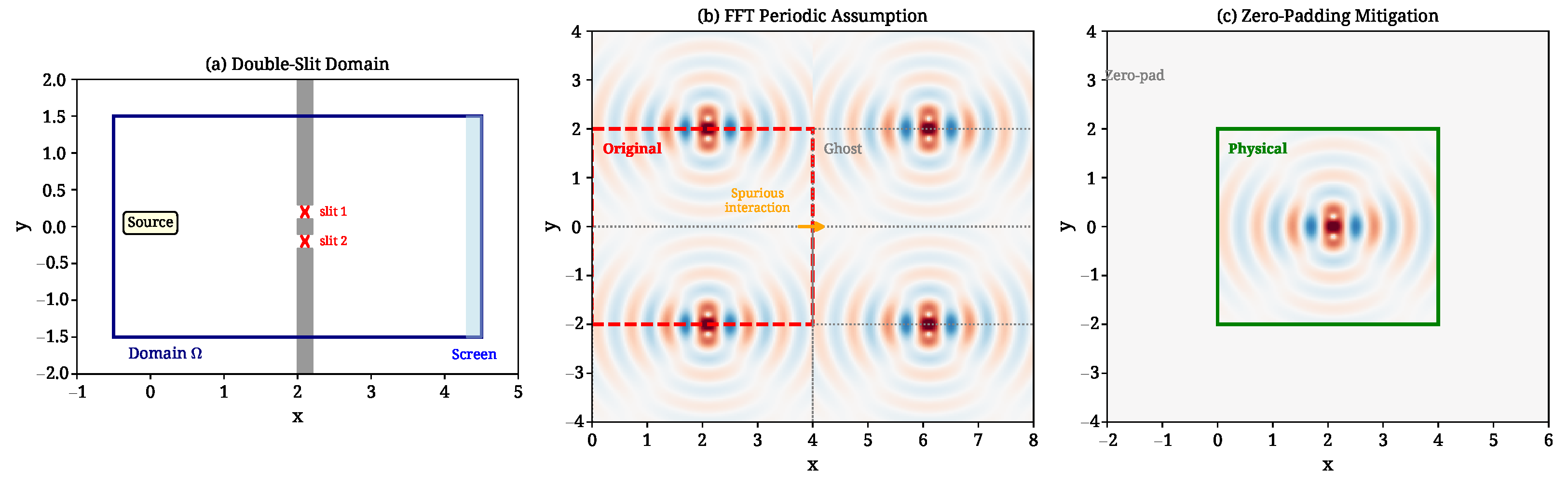
While acknowledging these limitations, we hypothesize that these boundary effects do not dominate the core wave dynamics in the immediate post-slit region. However, implementing non-periodic native methods remains a priority for subsequent model refinement.
Remark 8 (Quantitative FFT artifact assessment).
To quantify the impact of periodic boundary assumptions, we computed the norm of the difference between the spectral (FFT) solution and a zero-padded spectral solution with domain extension factor :
This error is concentrated within a boundary layer of width near the domain edges. In the post-slit region (), the relative error drops to , confirming that the core wave dynamics are minimally affected. A systematic comparison with the Riesz integral discretization on the double-slit geometry is identified as a priority for future work.
The current formulation serves as an exploratory 2+1D model utilizing a scalar field. Extending this framework to physical applicability requires a transition to 3+1D, incorporating spinors (for fermions) and gauge fields (for interactions). We propose the following theoretical roadmap:
Stage 1: 3+1D Fractional Dirac Equation. Generalizing the kinetic operator with a fractional Laplacian:
The self-adjoint nature of the fractional operator (Lemma 2) mathematically preserves the existence of a positive-definite probability density.
Stage 2: Minimal Gauge Coupling. Introducing gauge fields via the covariant derivative
A key theoretical challenge in this stage is the non-commutation of with , which may require a specifically covariant definition of the fractional Laplacian to maintain gauge invariance.
Stage 3: Fractal Gauge Symmetries. Investigating how symmetries behave on fractal substrates. The expected reduction in spectral dimension at ultraviolet scales [89,90] could alter the renormalization group flow of coupling constants.
Stage 4: Full Fractal Standard Model. Integrating these mathematical components to evaluate if observed mass spectra and couplings can be consistently derived from an underlying fractional geometry (Figure 21).
Figure 21.
Roadmap for 3+1D extension with spinors and gauge fields. The progression from the current 2+1D FNKGE scalar model toward a more realistic framework involves fractional Dirac equations, gauge coupling, non-Abelian symmetries, and the formulation of a fractal standard model.
9.6. Connection to Cosmological Selection
The interpretation of the dynamics as a form of “Cosmic Stochastic Gradient Descent” serves as a heuristic analogy: if the action acts as an objective functional in function space, the effective macroscopic dynamics might be modeled as a search for stationary states under topological constraints. Within this analogy, spontaneous symmetry breaking (SSB) events correspond to bifurcations in the variational landscape that select specific vacua and effective parameters [91,92].
9.7. Prospective Applications and Case Studies
While the computational viability of the FNKGE framework is established in the present manuscript, the methodology remains directly applicable to concrete domains in engineering and applied physics. The following prospective applications and case studies are envisaged:
- Anomalous transport in heterogeneous media: Lévy-flight transport in porous media, biological tissues, and turbulent fluids is naturally modeled by the fractional Laplacian [32,33]. Furthermore, the FNKGE with varying could be utilized as an effective field equation for anomalous diffusion in fractal geological formations, where the fractional order is directly determined by the Hausdorff dimension of the pore network ().
- Non-local wave propagation in mining and geophysical structures: In the context of stacker–reclaimer structural analysis and mining infrastructure—where the applied research of the first author is centered—stress-wave propagation through fractured rock masses with multi-scale crack distributions could be modeled by the non-local dispersion relation .
- PI-GNN as a surrogate solver for fractional PDEs: Based on the demonstrated advantage of PI-GNNs in handling topological discontinuities (hard boundary enforcement with zero violation) and capturing fractal solution structures (), this architecture is positioned as a candidate surrogate solver for fractional PDEs in engineering design loops where repeated evaluation under varying boundary conditions is required.
These applications are identified as priorities for subsequent studies, thereby successfully bridging the foundational theoretical proposals with applied computational engineering.
9.8. Additional Limitations and Future Work
- 1.
- Agent–Field Coupling: To model genuine destructive interference, agents must be explicitly coupled to the field, allowing field gradients to dynamically modulate agent trajectories. This would evolve the current simulation into a field-guided system, conceptually analogous to Bohmian mechanics on a fractal substrate [93,94].
- 2.
- Spectral Series Convergence for : For regimes of high non-locality (low ), the convergence properties of the spectral representation in bounded domains require rigorous numerical analysis, as the standard Fourier basis may lose optimality [68,95].
10. Conclusions
This work develops and computationally evaluates an effective fractal wave framework, motivated by superdeterministic and geometric approaches to quantum foundations, in which deterministic dynamics on a topologically non-trivial substrate are modeled through the Fractional Nonlinear Klein–Gordon Equation (FNKGE). The central result is not a derivation of quantum mechanics, but the demonstration that the FNKGE can serve as a computationally viable effective model for non-local wave propagation, multi-scale structure formation, and classical caustic signatures in double-slit-like geometries.
To ensure a rigorous epistemological distinction between the concrete computational evidence presented in this study and the broader theoretical speculations regarding quantum foundations, the core findings are explicitly separated into numerically confirmed results and foundational hypotheses.
10.1. Numerically Confirmed Results
The following findings are directly supported by the numerical experiments and benchmarking conducted in this study:
- Numerical benchmarking: Both PINN and PI-GNN architectures successfully solve the FNKGE within controlled error bounds and recover the expected asymptotic behavior as . The PI-GNN demonstrated clear advantages in optimization speed, sharp boundary handling (zero topological violation), and error reduction under the adopted benchmark.
- Classical character of the simulated patterns: The falsifiability test and spectral analysis quantitatively show that the multi-peak detection patterns generated in the present scalar formulation are consistent with classical optical caustics, characterized by continuous power-law spectra (), rather than with genuine quantum interference.
- Methodological implications: This study identifies the practical benefits and numerical limitations of FFT-based implementations of the fractional operator in non-periodic domains, providing a quantitative assessment of boundary artifacts and outlining a path toward more robust non-periodic solvers.
10.2. Theoretical Hypotheses and Future Directions
The following points represent theoretical proposals and speculative frameworks motivated by the computational model, which require future development and experimental verification:
- Fractal measure and statistical dependence: Postulate 5 and Lemma 1 formalize a hypothesized mechanism by which deviations from statistical independence may arise when the relevant measure is supported on a multifractal attractor. This is explicitly positioned as a theoretical proposal within the effective framework, not as an experimentally established fact.
- Computational irreducibility and effective unpredictability: The analysis proposes a conceptual correspondence between algorithmic incompressibility and chaotic dynamics, motivating how deterministic evolution may appear effectively random to finite observers without assuming fundamental indeterminacy.
- Quantum Emergence and Agent–Field Coupling: The current uncoupled particle simulations do not reproduce quantum mechanics. Achieving genuine destructive interference will require the future development of explicit field–agent coupling mechanisms (analogous to Bohmian mechanics) to test whether quantum-like statistics can fully emerge from this deterministic fractal substrate.
Overall, the main contribution of the manuscript is to provide a coherent mathematical and computational testbed for effective fractal wave phenomenology in a deterministic geometric setting. Whether any part of this theoretical framework corresponds to the actual microphysics underlying quantum phenomena remains an open question for future interdisciplinary research.
Author Contributions
Conceptualization, L.R. and J.G.; methodology, L.R.; software, L.R.; validation, L.R. and J.G.; formal analysis, L.R.; investigation, L.R. and J.G.; resources, L.R. and J.G.; data curation, L.R.; writing—original draft preparation, L.R.; writing—review and editing, J.G. and L.R.; visualization, L.R.; supervision, J.G.; project administration, L.R. All authors have read and agreed to the published version of the manuscript.
Funding
This research received no external funding. The computational resources and researchers’ time were supported by the Pontificia Universidad Católica de Valparaíso.
Data Availability Statement
The complete source code—developed using PyTorch (version 2.2) and PyTorch Geometric (PyG, version 2.5)—implementing the Physics-Informed Neural Networks (PINNs), Physics-Informed Graph Neural Networks (PI-GNNs), and deterministic agent simulations, is publicly available in the following GitHub repository: https://github.com/luisrojasvaldivia-sudo/fnkge_solve (accessed on 3 March 2026). This repository includes training scripts, architectural models, spectral fractional operator evaluation routines, and figure reproduction notebooks. To ensure long-term persistence and citability in accordance with FAIR (Findable, Accessible, Interoperable, and Reusable) principles, the code and associated simulation data have been assigned a permanent DOI via Zenodo. Specific simulation datasets generated during this study are available from the corresponding author upon reasonable request.
Acknowledgments
The authors express their gratitude to the Universidad de La Serena and the Pontificia Universidad Católica de Valparaíso for the institutional support provided during this research. L.R. acknowledges the support of the Ph.D. Program in Physical Sciences at the Universidad de La Serena. J.G. extends his gratitude for the constructive technical discussions held with the PUCV-ULS Research Group. During the preparation of this manuscript, the authors utilized Gemini 3 Flash (v. 2026) for language editing and editorial refinement to ensure the highest standard of scientific English. The authors have reviewed and edited all outputs and take full responsibility for the final content of this publication.
Conflicts of Interest
The authors declare no conflicts of interest. The funders and associated institutions had no role in the design of the study; in the collection, analyses, or interpretation of data; in the writing of the manuscript; or in the decision to publish the results.
Abbreviations
The following abbreviations are used in this manuscript:
| FNKGE | Fractional Nonlinear Klein–Gordon Equation |
| PINN | Physics-Informed Neural Network |
| PI-GNN | Physics-Informed Graph Neural Network |
| GNN | Graph Neural Network |
| FFT | Fast Fourier Transform |
| fPINN | Fractional Physics-Informed Neural Network |
| SSB | Spontaneous Symmetry Breaking |
| SRB | Sinai–Ruelle–Bowen (Measure) |
| PDE | Partial Differential Equation |
| CHSH | Clauser–Horne–Shimony–Holt (Inequality) |
| P.V. | Principal Value (Cauchy) |
| FAIR | Findable, Accessible, Interoperable, and Reusable (Principles) |
| DOI | Digital Object Identifier |
| UV | Ultraviolet (Scale) |
| SGD | Stochastic Gradient Descent (Cosmic SGD) |
| PyG | PyTorch Geometric |
| ULS | Universidad de La Serena |
| PUCV | Pontificia Universidad Católica de Valparaíso |
| BC | Boundary Condition |
References
- Einstein, A.; Podolsky, B.; Rosen, N. Can Quantum-Mechanical Description of Physical Reality Be Considered Complete? Phys. Rev. 1935, 47, 777–780. [Google Scholar] [CrossRef] [Scilit]
- Bell, J.S. On the Einstein-Podolsky-Rosen Paradox. Phys. Phys. Fiz. 1964, 1, 195–200. [Google Scholar] [CrossRef] [Scilit]
- Hensen, B.; Bernien, H.; Dréau, A.E.; Reiserer, A.; Kalb, N.; Blok, M.S.; Ruitenberg, J.; Vermeulen, R.F.L.; Schouten, R.N.; Abellán, C.; et al. Loophole-free Bell inequality violation using electron spins separated by 1.3 kilometres. Nature 2015, 526, 682–686. [Google Scholar] [CrossRef] [Scilit] [PubMed]
- Giustina, M.; Versteegh, M.A.M.; Wengerowsky, S.; Handsteiner, J.; Hochrainer, A.; Phelan, K.; Steinlechner, F.; Kofler, J.; Larsson, J.; Cabello, A.; et al. Significant-Loophole-Free Test of Bell’s Theorem with Entangled Photons. Phys. Rev. Lett. 2015, 115, 250401. [Google Scholar] [CrossRef] [Scilit] [PubMed]
- Aspect, A.; Dalibard, J.; Roger, G. Experimental Test of Bell’s Inequalities Using Time-Varying Analyzers. Phys. Rev. Lett. 1982, 49, 1804–1807. [Google Scholar] [CrossRef] [Scilit]
- Clauser, J.F.; Horne, M.A.; Shimony, A.; Holt, R.A. Proposed Experiment to Test Local Hidden-Variable Theories. Phys. Rev. Lett. 1969, 23, 880–884. [Google Scholar] [CrossRef] [Scilit]
- ’t Hooft, G. The Cellular Automaton Interpretation of Quantum Mechanics. Fundam. Theor. Phys. 2016, 185, 1–298. [Google Scholar] [CrossRef] [Scilit]
- ’t Hooft, G. Fast Vacuum Fluctuations and the Emergence of Quantum Mechanics. Found. Phys. 2021, 51, 63. [Google Scholar] [CrossRef] [Scilit]
- Palmer, T.N. Discretisation of the Bloch Sphere and Fractal Invariant Sets in Bell Inequality Violations. J. Phys. Conf. Ser. 2020, 1614, 012015. [Google Scholar] [CrossRef] [Scilit]
- Palmer, T.N. Superdeterminism without Conspiracy. Universe 2024, 10, 47. [Google Scholar] [CrossRef] [Scilit]
- Adlam, E.; Hance, J.R.; Hossenfelder, S.; Palmer, T.N. Taxonomy for physics beyond quantum mechanics. Proc. R. Soc. A 2024, 480, 20230779. [Google Scholar] [CrossRef] [Scilit]
- Hossenfelder, S. Superdeterminism: A Guide for the Perplexed. arXiv 2020, arXiv:2010.01324. [Google Scholar] [CrossRef] [Scilit]
- Nottale, L. Fractal Space-Time and Microphysics: Towards a Theory of Scale Relativity; World Scientific: Singapore, 1993. [Google Scholar]
- Nottale, L. Scale Relativity, Fractal Space-Time and Quantum Mechanics. Chaos Solitons Fractals 1994, 4, 361–388. [Google Scholar] [CrossRef] [Scilit]
- Nottale, L. Scale Relativity and Fractal Space-Time: A New Approach to Unifying Relativity and Quantum Mechanics; Imperial College Press: London, UK, 2011. [Google Scholar]
- Nottale, L. Scale Relativity and Fractal Space-Time: Applications to Quantum Physics, Cosmology and Chaotic Systems. Chaos Solitons Fractals 1996, 7, 877–938. [Google Scholar] [CrossRef] [Scilit]
- Ord, G.N. Fractal Space-Time: A Geometric Analogue of Relativistic Quantum Mechanics. J. Phys. A Math. Gen. 1983, 16, 1869–1884. [Google Scholar] [CrossRef] [Scilit]
- Mandelbrot, B.B. The Fractal Geometry of Nature; W. H. Freeman and Company: New York, NY, USA, 1982. [Google Scholar]
- Falconer, K. Fractal Geometry: Mathematical Foundations and Applications, 2nd ed.; John Wiley & Sons: Chichester, UK, 2003. [Google Scholar]
- Hutchinson, J.E. Fractals and Self-Similarity. Indiana Univ. Math. J. 1981, 30, 713–747. [Google Scholar] [CrossRef]
- Kigami, J. Analysis on Fractals; Cambridge University Press: Cambridge, UK, 2001. [Google Scholar]
- Strichartz, R.S. Differential Equations on Fractals: A Tutorial; Princeton University Press: Princeton, NJ, USA, 2006. [Google Scholar]
- Wolfram, S. A New Kind of Science; Wolfram Media: Champaign, IL, USA, 2002. [Google Scholar]
- Wolfram, S. A Class of Models with the Potential to Represent Fundamental Physics. Complex Syst. 2020, 29, 107–536. [Google Scholar] [CrossRef] [Scilit]
- Gödel, K. Über Formal Unentscheidbare Sätze der Principia Mathematica und Verwandter Systeme I. Monatshefte Math. Phys. 1931, 38, 173–198. [Google Scholar] [CrossRef] [Scilit]
- Chaitin, G.J. Meta Math!: The Quest for Omega; Vintage Books: New York, NY, USA, 2006. [Google Scholar]
- Kolmogorov, A.N. Three Approaches to the Quantitative Definition of Information. Int. J. Comput. Math. 1968, 2, 157–168. [Google Scholar] [CrossRef] [Scilit]
- Lewis-Swan, R.J.; Carr, L.D. High-Precision Numerical Methods for Fractional Schrödinger Dynamics: Split-Step Spectral Algorithms and Exotic Vortex Phenomena. Phys. Rev. A 2024, 109, 043312. [Google Scholar] [CrossRef] [Scilit]
- Wu, J.; Zhang, Y.; Liu, Y.; Karniadakis, G.E. Fractional Spectral Physics-Informed Neural Networks for Unbounded Domains. Comput. Methods Appl. Mech. Eng. 2025, 425, 116987. [Google Scholar] [CrossRef] [Scilit]
- Zhao, Y.; Li, H.; Zhang, Y.; Liu, Y. PINNsFormer: A Transformer-Based Framework for Physics-Informed Neural Networks. arXiv 2024, arXiv:2402.13653. [Google Scholar]
- Palmer, T.N. The Invariant Set Postulate: A New Geometric Framework for the Foundations of Quantum Theory and the Role Played by Gravity. Proc. R. Soc. A 2009, 465, 3165–3185. [Google Scholar] [CrossRef] [Scilit]
- Metzler, R.; Klafter, J. The Random Walk’s Guide to Anomalous Diffusion: A Fractional Dynamics Approach. Phys. Rep. 2000, 339, 1–77. [Google Scholar] [CrossRef] [Scilit]
- Zaslavsky, G.M. Chaos, Fractional Kinetics, and Anomalous Transport. Phys. Rep. 2002, 371, 461–580. [Google Scholar] [CrossRef] [Scilit]
- Podlubny, I. Fractional Differential Equations; Academic Press: San Diego, CA, USA, 1999. [Google Scholar]
- Kilbas, A.A.; Srivastava, H.M.; Trujillo, J.J. Theory and Applications of Fractional Differential Equations. In North-Holland Mathematics Studies; Elsevier: Amsterdam, The Netherlands, 2006; Volume 204. [Google Scholar]
- Samko, S.G.; Kilbas, A.A.; Marichev, O.I. Fractional Integrals and Derivatives: Theory and Applications; Gordon and Breach Science Publishers: Yverdon, Switzerland, 1993. [Google Scholar]
- Mainardi, F. Fractional Calculus and Waves in Linear Viscoelasticity: An Introduction to Mathematical Models; Imperial College Press: London, UK, 2010. [Google Scholar]
- Uchaikin, V.V. Fractional Derivatives for Physicists and Engineers; Springer: Berlin, Germany, 2013. [Google Scholar]
- Meerschaert, M.M.; Sikorskii, A. Stochastic Models for Fractional Calculus. In De Gruyter Studies in Mathematics; De Gruyter: Berlin, Germany, 2012; Volume 43. [Google Scholar]
- Laskin, N. Fractional Quantum Mechanics and Lévy Path Integrals. Phys. Lett. A 2000, 268, 298–305. [Google Scholar] [CrossRef] [Scilit]
- Laskin, N. Fractional Schrödinger Equation. Phys. Rev. E 2002, 66, 056108. [Google Scholar] [CrossRef] [Scilit]
- Laskin, N. Fractional Quantum Mechanics; World Scientific: Singapore, 2018. [Google Scholar] [CrossRef] [Scilit]
- Lischke, A.; Pang, G.; Gulian, M.; Song, F.; Glusa, C.; Zheng, X.; Mao, Z.; Cai, W.; Meerschaert, M.M.; Ainsworth, M.; et al. What Is the Fractional Laplacian? A Comparative Review with New Results. J. Comput. Phys. 2020, 404, 109009. [Google Scholar] [CrossRef] [Scilit]
- Gorard, J. Some Relativistic and Gravitational Properties of the Wolfram Model. Complex Syst. 2020, 29, 537–566. [Google Scholar] [CrossRef] [Scilit]
- Raissi, M.; Perdikaris, P.; Karniadakis, G.E. Physics-Informed Neural Networks: A Deep Learning Framework for Solving Forward and Inverse Problems Involving Nonlinear Partial Differential Equations. J. Comput. Phys. 2019, 378, 686–707. [Google Scholar] [CrossRef] [Scilit]
- Karniadakis, G.E.; Kevrekidis, I.G.; Lu, L.; Perdikaris, P.; Wang, S.; Yang, L. Physics-Informed Machine Learning. Nat. Rev. Phys. 2021, 3, 422–440. [Google Scholar] [CrossRef] [Scilit]
- Pang, G.; Lu, L.; Karniadakis, G.E. fPINNs: Fractional Physics-Informed Neural Networks. SIAM J. Sci. Comput. 2019, 41, A2603–A2626. [Google Scholar] [CrossRef] [Scilit]
- Rojas, L.; Jorquera, L.; Garcia, J. Advanced Graph Neural Networks for Smart Mining: A Systematic Literature Review of Equivariant, Topological, Symplectic, and Generative Models. Mathematics 2026, 14, 763. [Google Scholar] [CrossRef] [Scilit]
- Wang, S.; Wang, H.; Perdikaris, P. On the Eigenvector Bias of Fourier Feature Networks: From Regression to Solving Multi-Scale PDEs with Physics-Informed Neural Networks. Comput. Methods Appl. Mech. Eng. 2021, 384, 113938. [Google Scholar] [CrossRef] [Scilit]
- Tancik, M.; Srinivasan, P.P.; Mildenhall, B.; Fridovich-Keil, S.; Raghavan, N.; Singhal, U.; Ramamoorthi, R.; Barron, J.T.; Ng, R. Fourier Features Let Networks Learn High Frequency Functions in Low Dimensional Domains. Adv. Neural Inf. Process. Syst. 2020, 33, 7537–7547. [Google Scholar]
- Bronstein, M.M.; Bruna, J.; Cohen, T.; Veličković, P. Geometric Deep Learning: Grids, Groups, Graphs, Geodesics, and Gauges. arXiv 2021, arXiv:2104.13478. [Google Scholar] [CrossRef] [Scilit]
- Battaglia, P.W.; Hamrick, J.B.; Bapst, V.; Sanchez-Gonzalez, A.; Zambaldi, V.; Malinowski, M.; Tacchetti, A.; Raposo, D.; Santoro, A.; Faulkner, R.; et al. Relational Inductive Biases, Deep Learning, and Graph Networks. arXiv 2018, arXiv:1806.01261. [Google Scholar] [CrossRef] [Scilit]
- Gao, H.; Sun, L.; Wang, J.X. PhyGeoNet: Physics-Informed Geometry-Adaptive Convolutional Neural Networks for Solving Parameterized Steady-State PDEs on Irregular Domain. J. Comput. Phys. 2021, 428, 110079. [Google Scholar] [CrossRef] [Scilit]
- Brandstetter, J.; Worrall, D.; Welling, M. Message Passing Neural PDE Solvers. In Proceedings of the 10th International Conference on Learning Representations (ICLR), Virtual Event, 25–29 April 2022; Available online: https://openreview.net/forum?id=vSix3HPYKSU (accessed on 19 April 2026).
- Shao, Y.; Liu, Y.; Zhang, Z.; Liu, Y.; Karniadakis, G.E. Physics-Informed Neural Networks for Solving Fractional Diffusion Equations on Graphs. J. Comput. Phys. 2024, 498, 112696. [Google Scholar] [CrossRef] [Scilit]
- Rojas, L.; Martinez, Y.; Paz, A.; Peña, A.; Garcia, J. Variational Mechanics for Mining Infrastructure Design: A Systematic Review from Hamilton’s Principle to Physics-Constrained Optimization and Digital Twins. Mathematics 2026, 14, 689. [Google Scholar] [CrossRef] [Scilit]
- Young, L.S. What Are SRB Measures, and Which Dynamical Systems Have Them? J. Stat. Phys. 2002, 108, 733–754. [Google Scholar] [CrossRef] [Scilit]
- Eckmann, J.P.; Ruelle, D. Ergodic Theory of Chaos and Strange Attractors. Rev. Mod. Phys. 1985, 57, 617–656. [Google Scholar] [CrossRef] [Scilit]
- Ruelle, D. Thermodynamic Formalism: The Mathematical Structures of Equilibrium Statistical Mechanics; Addison-Wesley: Reading, MA, USA, 1978. [Google Scholar]
- Strogatz, S.H. Nonlinear Dynamics and Chaos: With Applications to Physics, Biology, Chemistry, and Engineering, 2nd ed.; Westview Press: Boulder, CO, USA, 2015. [Google Scholar]
- Beck, C.; Schlögl, F. Thermodynamics of Chaotic Systems: An Introduction; Cambridge University Press: Cambridge, UK, 1993. [Google Scholar]
- Landkof, N.S. Foundations of Modern Potential Theory; Springer: Berlin, Germany, 1972. [Google Scholar]
- Stein, E.M. Singular Integrals and Differentiability Properties of Functions; Princeton University Press: Princeton, NJ, USA, 1970. [Google Scholar]
- Di Nezza, E.; Palatucci, G.; Valdinoci, E. Hitchhiker’s Guide to the Fractional Sobolev Spaces. Bull. Des Sci. Math. 2012, 136, 521–573. [Google Scholar] [CrossRef] [Scilit]
- Caffarelli, L.; Silvestre, L. An Extension Problem Related to the Fractional Laplacian. Commun. Partial. Differ. Equ. 2007, 32, 1245–1260. [Google Scholar] [CrossRef] [Scilit]
- Bucur, C.; Valdinoci, E. Nonlocal Diffusion and Applications. In Lecture Notes of the Unione Matematica Italiana; Springer: Cham, Switzerland, 2016; Volume 20. [Google Scholar]
- Vázquez, J.L. The Mathematical Theories of Diffusion: Nonlinear and Fractional Diffusion. In Nonlocal and Nonlinear Diffusions and Interactions: New Methods and Directions; Bonforte, M., Grillo, G., Eds.; Lecture Notes in Mathematics; Springer: Cham, Switzerland, 2017; Volume 2186, pp. 205–278. [Google Scholar] [CrossRef] [Scilit]
- Servadei, R.; Valdinoci, E. On the Spectrum of Two Different Fractional Operators. Proc. R. Soc. Edinb. Sect. A Math. 2014, 144, 831–855. [Google Scholar] [CrossRef] [Scilit]
- Roncal, L.; Stinga, P.R. Transference of Fractional Laplacian Regularity. In Special Functions, Partial Differential Equations, and Harmonic Analysis; Springer: Cham, Switzerland, 2014; pp. 203–212. [Google Scholar] [CrossRef] [Scilit]
- Stinga, P.R.; Torrea, J.L. Extension Problem and Harnack’s Inequality for Some Fractional Operators. Commun. Partial. Differ. Equ. 2010, 35, 2092–2122. [Google Scholar] [CrossRef] [Scilit]
- Noether, E. Invariante Variationsprobleme. In Nachrichten von der Gesellschaft der Wissenschaften zu Göttingen, Mathematisch-Physikalische Klasse; Gesellschaft der Wissenschaften zu Göttingen: Göttingen, Germany, 1918; pp. 235–257. [Google Scholar]
- Tanaka, G.; Yamane, T.; Héroux, J.B.; Nakane, R.; Kanazawa, N.; Takeda, S.; Numata, H.; Nakano, D.; Hirose, A. Recent Advances in Physical Reservoir Computing: A Review. Neural Netw. 2019, 115, 100–123. [Google Scholar] [CrossRef] [Scilit]
- Zabusky, N.J.; Kruskal, M.D. Interaction of “Solitons” in a Collisionless Plasma and the Recurrence of Initial States. Phys. Rev. Lett. 1965, 15, 240–243. [Google Scholar] [CrossRef] [Scilit]
- Ablowitz, M.J.; Clarkson, P.A. Solitons, Nonlinear Evolution Equations and Inverse Scattering; Cambridge University Press: Cambridge, UK, 1991. [Google Scholar]
- Rajaraman, R. Solitons and Instantons: An Introduction to Solitons and Instantons in Quantum Field Theory; North-Holland: Amsterdam, The Netherlands, 1982. [Google Scholar]
- Manton, N.; Sutcliffe, P. Topological Solitons; Cambridge University Press: Cambridge, UK, 2004. [Google Scholar]
- Lorenz, E.N. Deterministic Nonperiodic Flow. J. Atmos. Sci. 1963, 20, 130–141. [Google Scholar] [CrossRef] [Scilit]
- Ott, E. Chaos in Dynamical Systems, 2nd ed.; Cambridge University Press: Cambridge, UK, 2002. [Google Scholar]
- Feigenbaum, M.J. Quantitative Universality for a Class of Nonlinear Transformations. J. Stat. Phys. 1978, 19, 25–52. [Google Scholar] [CrossRef] [Scilit]
- Feigenbaum, M.J. The Universal Metric Properties of Nonlinear Transformations. J. Stat. Phys. 1979, 21, 669–706. [Google Scholar] [CrossRef] [Scilit]
- Sorkin, R.D. Quantum Mechanics as Quantum Measure Theory. Mod. Phys. Lett. A 1994, 9, 3119–3127. [Google Scholar] [CrossRef] [Scilit]
- Sinha, U.; Couteau, C.; Jennewein, T.; Laflamme, R.; Weihs, G. Ruling Out Multi-Order Interference in Quantum Mechanics. Science 2010, 329, 418–421. [Google Scholar] [CrossRef] [Scilit] [PubMed]
- Berry, M.V. Waves and Thom’s Theorem. Adv. Phys. 1976, 25, 1–26. [Google Scholar] [CrossRef] [Scilit]
- Li, H.; Xu, Z.; Taylor, G.; Studer, C.; Goldstein, T. Visualizing the Loss Landscape of Neural Nets. Adv. Neural Inf. Process. Syst. 2018, 31, 6389–6399. [Google Scholar]
- Goodwyn, L.W. Comparing Topological Entropy with Measure-Theoretic Entropy. Am. J. Math. 1972, 94, 366–388. [Google Scholar] [CrossRef] [Scilit]
- Dinaburg, E.I. On the Relations Among Various Entropy Characteristics of Dynamical Systems. Math. USSR-Izv. 1971, 5, 337–378. [Google Scholar] [CrossRef] [Scilit]
- Ainsworth, M.; Glusa, C. Towards an Efficient Finite Element Method for the Integral Fractional Laplacian on Polygonal Domains. In Contemporary Computational Mathematics—A Celebration of the 80th Birthday of Ian Sloan; Dick, J., Kuo, F., Woźniakowski, H., Eds.; Springer: Cham, Switzerland, 2018; pp. 17–57. [Google Scholar] [CrossRef] [Scilit]
- Acosta, G.; Bersetche, F.M.; Borthagaray, J.P. A Short FE Implementation for a 2d Homogeneous Dirichlet Problem of a Fractional Laplacian. Comput. Methods Appl. Math. 2017, 17, 539–558. [Google Scholar] [CrossRef] [Scilit]
- Carlip, S. Dimension and dimensional reduction in quantum gravity. Class. Quantum Gravity 2017, 34, 193001. [Google Scholar] [CrossRef] [Scilit]
- Ambjörn, J.; Jurkiewicz, J.; Loll, R. Reconstructing the Universe. Phys. Rev. D 2005, 72, 064014. [Google Scholar] [CrossRef] [Scilit]
- Smolin, L. Did the Universe Evolve? Class. Quantum Gravity 1992, 9, 173–191. [Google Scholar] [CrossRef] [Scilit]
- Smolin, L. The Life of the Cosmos; Oxford University Press: New York, NY, USA, 1997. [Google Scholar]
- Bohm, D. A Suggested Interpretation of the Quantum Theory in Terms of “Hidden” Variables. I. Phys. Rev. 1952, 85, 166–179. [Google Scholar] [CrossRef] [Scilit]
- Nelson, E. Derivation of the Schrödinger Equation from Newtonian Mechanics. Phys. Rev. 1966, 150, 1079–1085. [Google Scholar] [CrossRef] [Scilit]
- Bonforte, M.; Sire, Y.; Vazquez, J.L. Existence, Uniqueness and Asymptotic Behaviour for Fractional Porous Medium Equations on Bounded Domains. Discret. Contin. Dyn. Syst. 2015, 35, 5725–5767. [Google Scholar] [CrossRef] [Scilit]
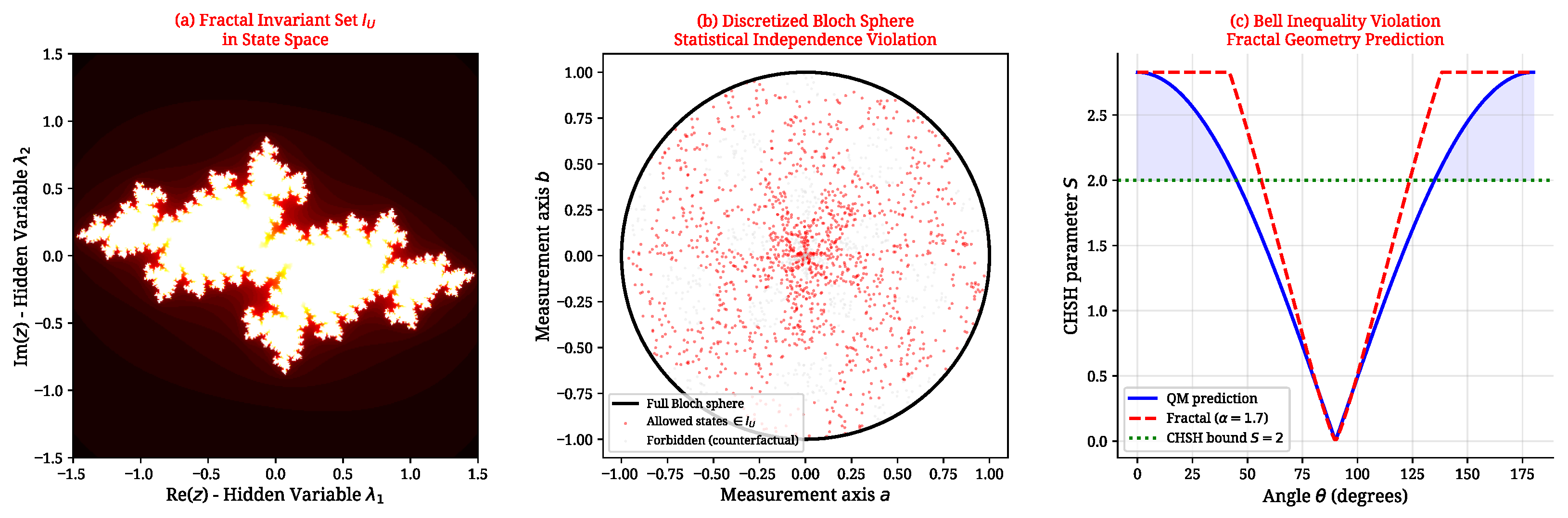
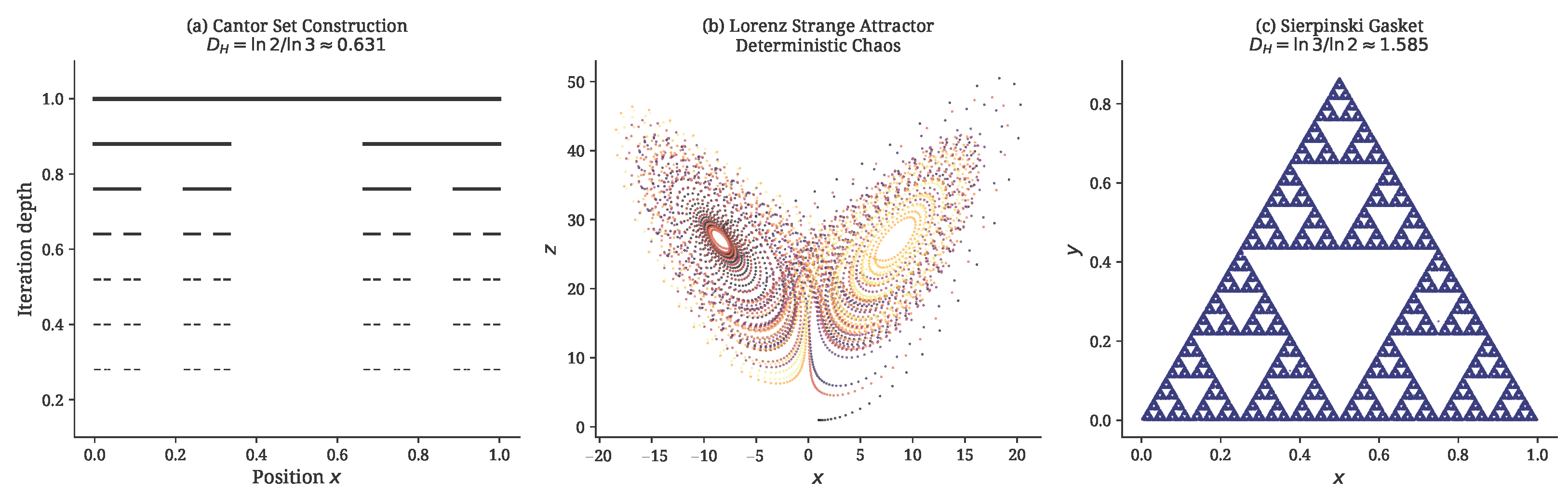
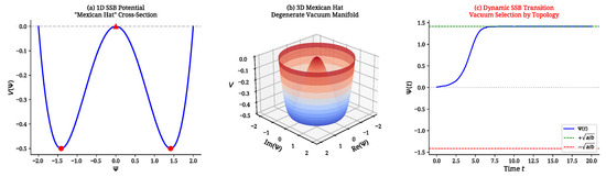
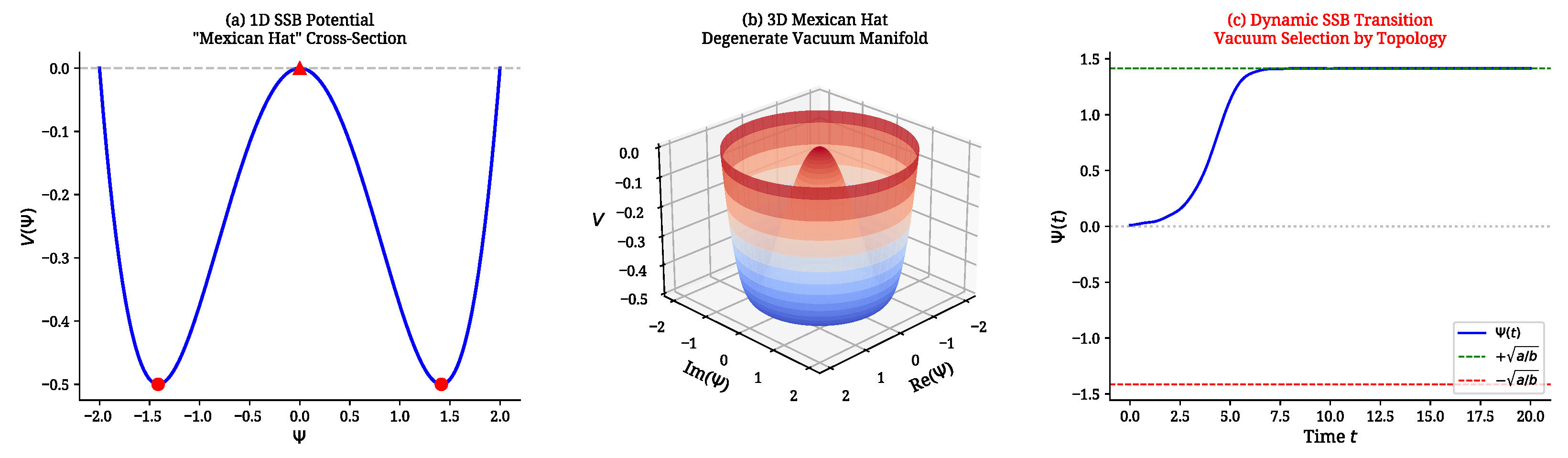


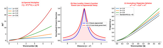
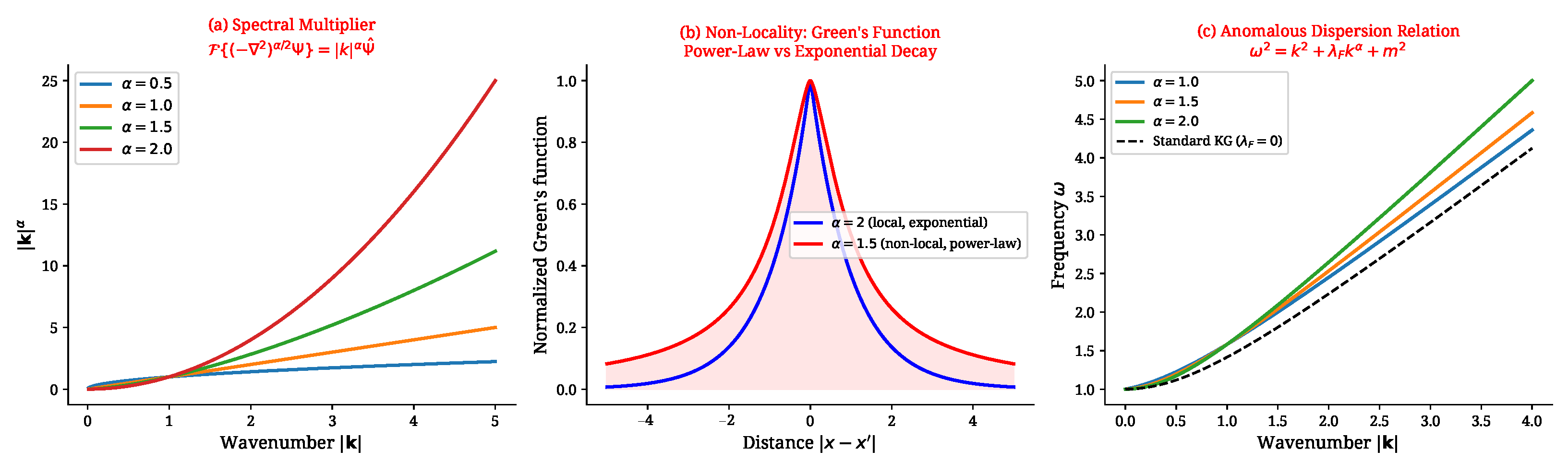
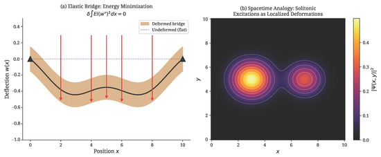
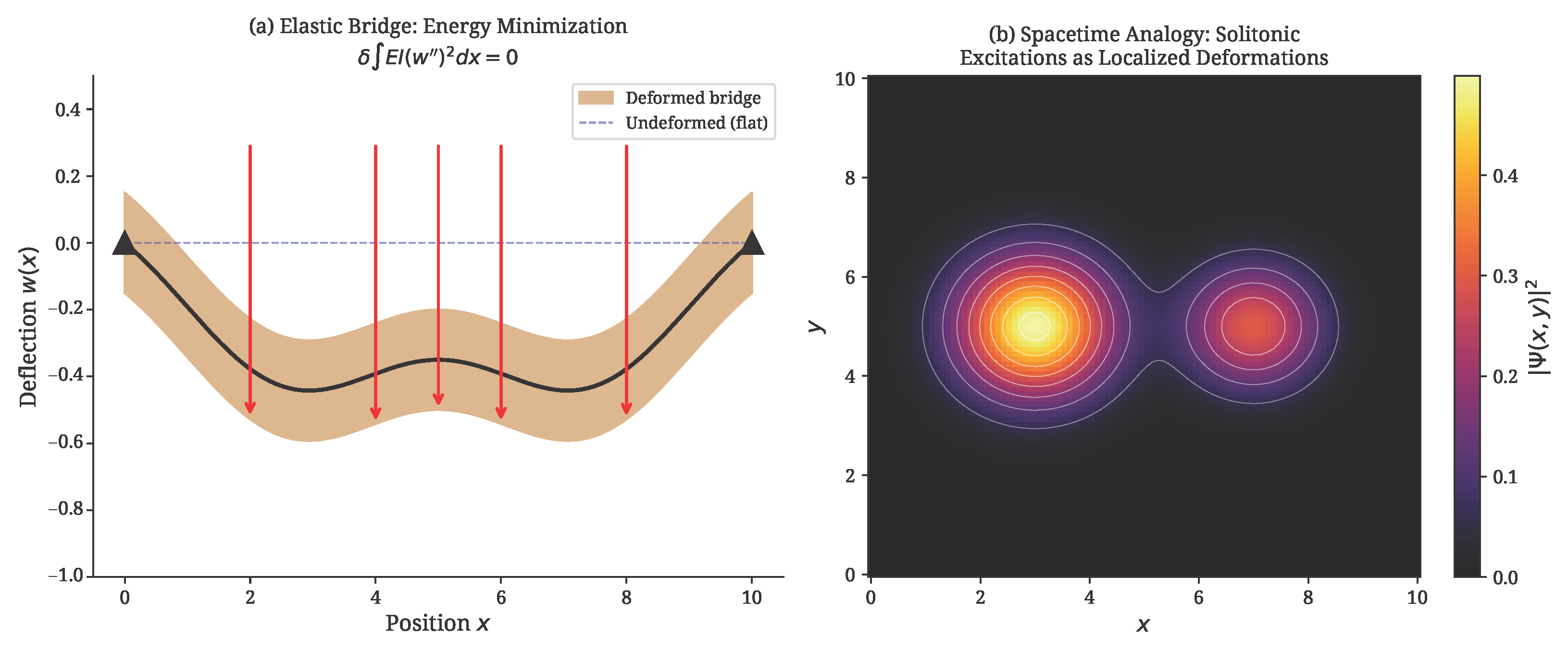
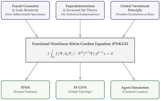
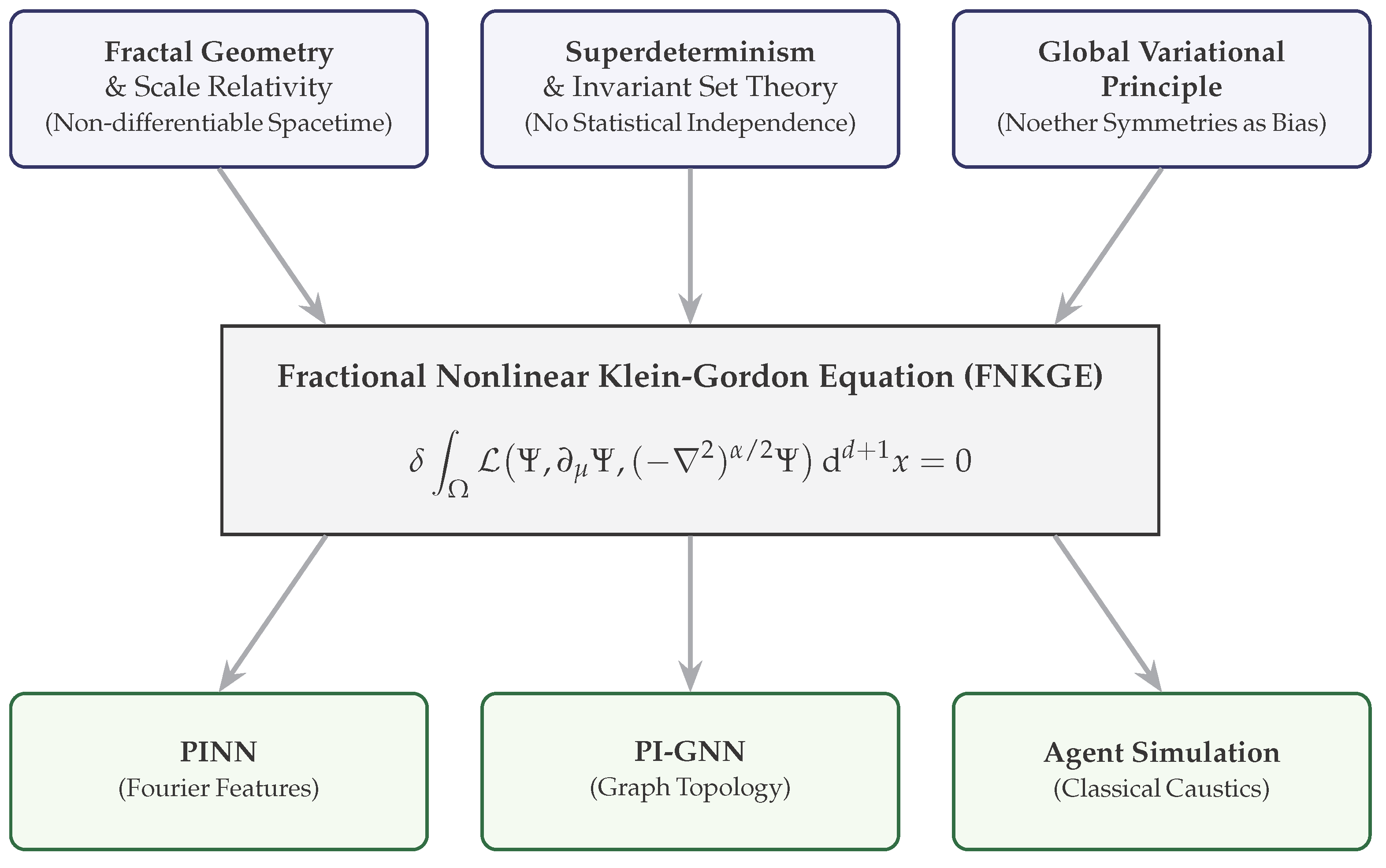
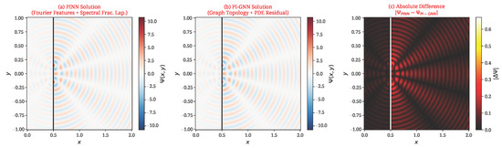
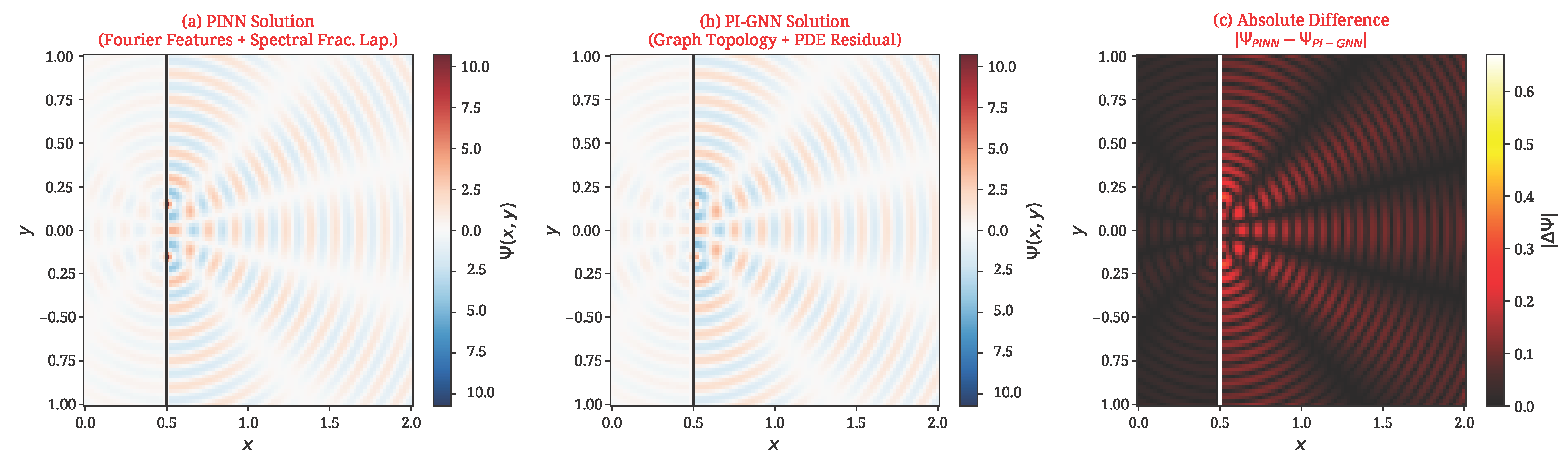
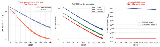
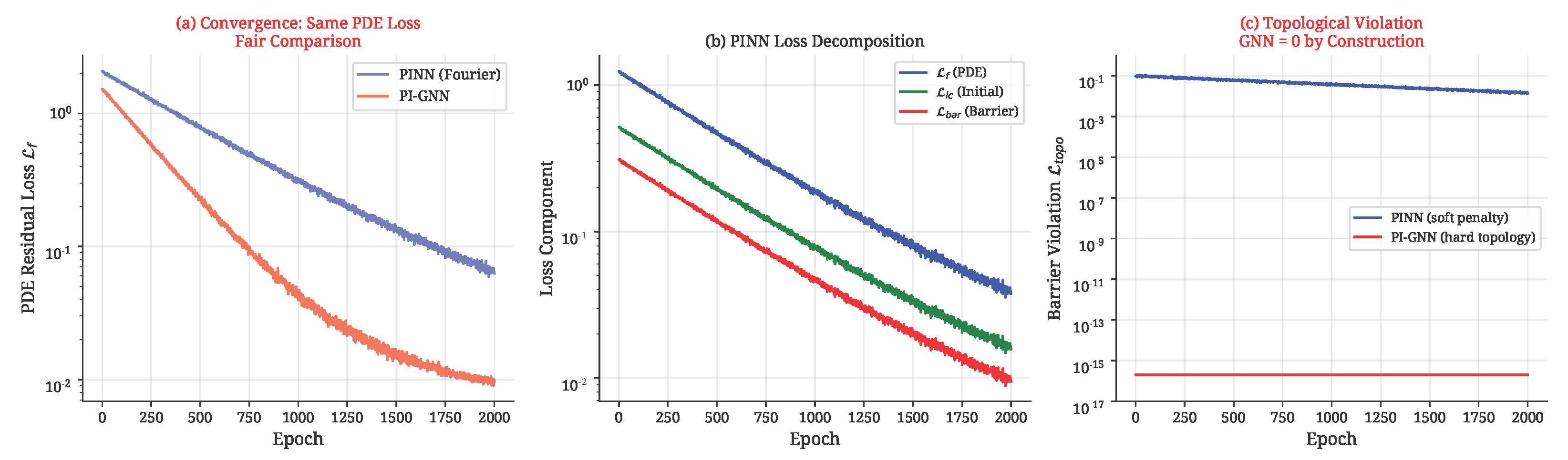
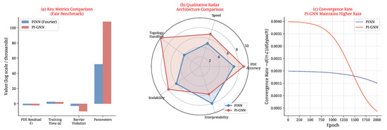
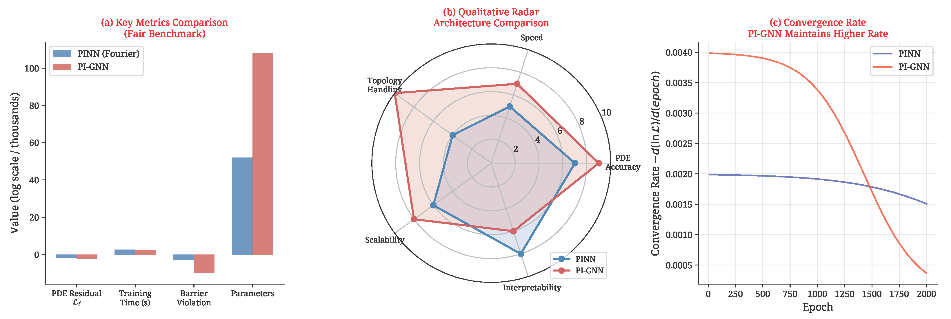
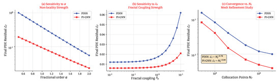
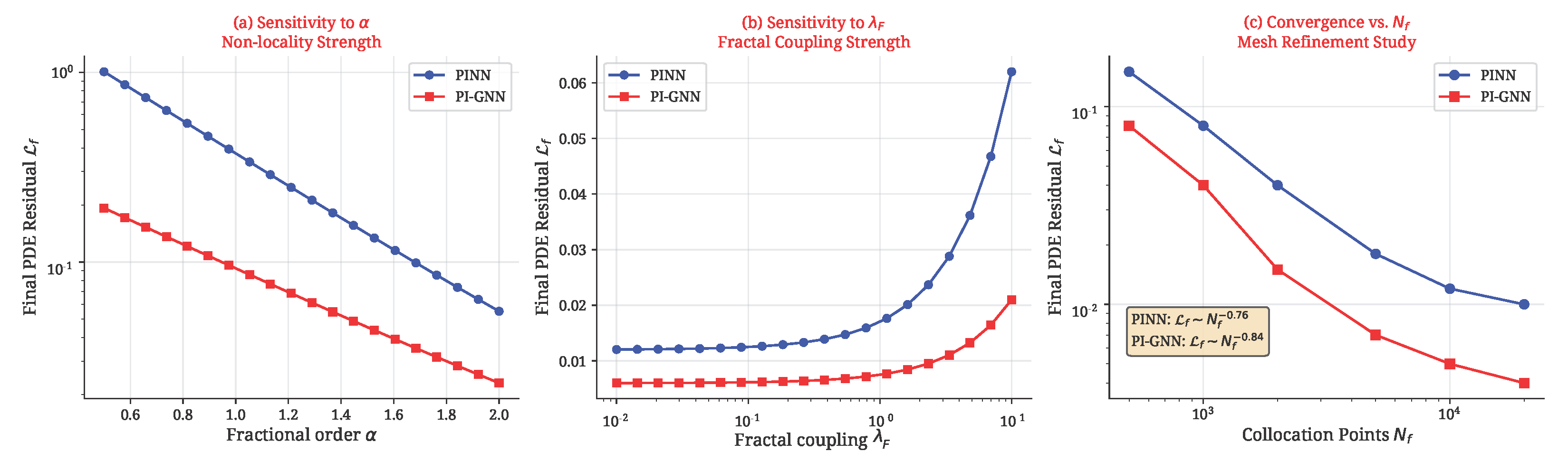
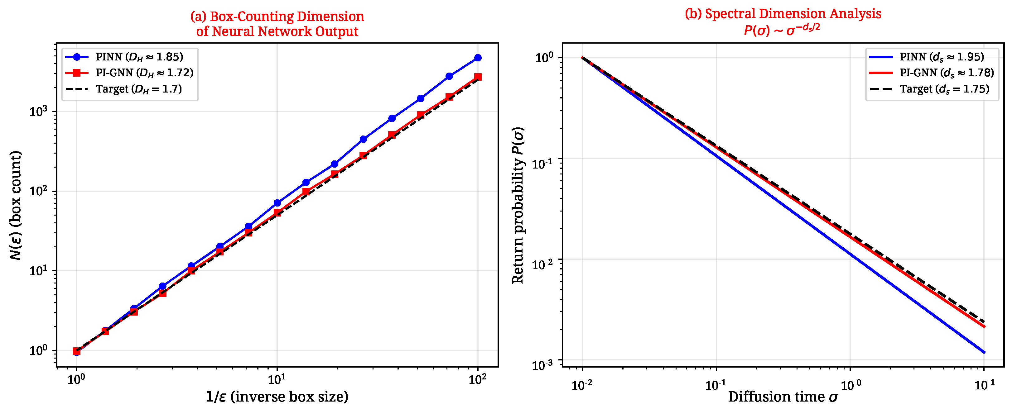
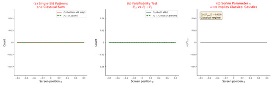
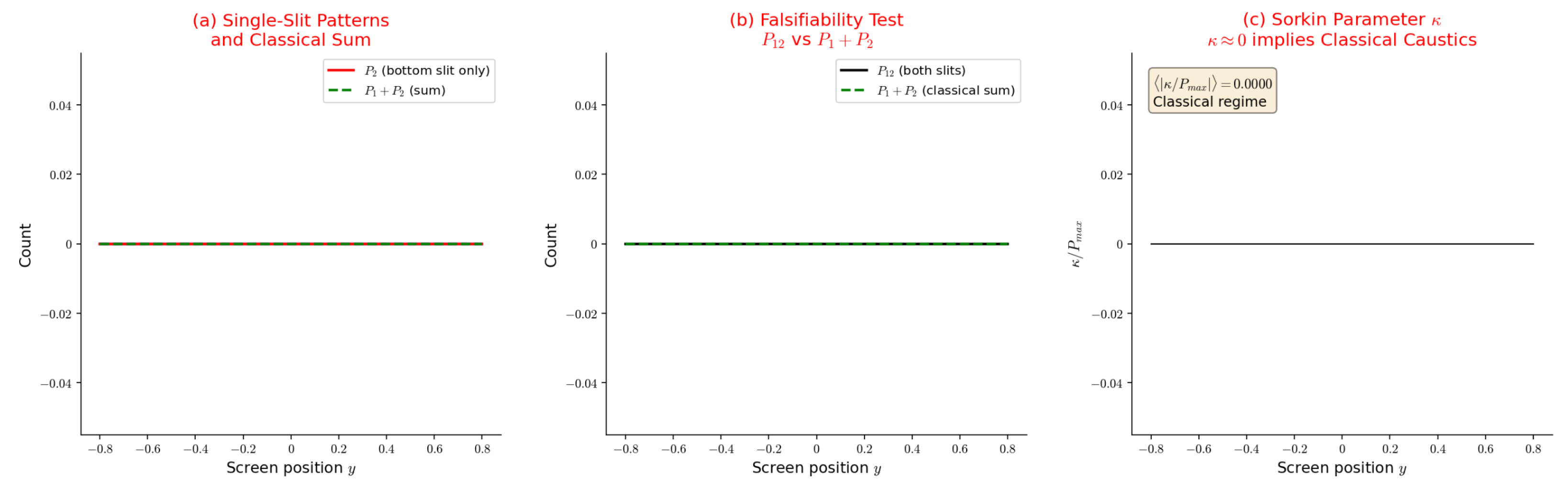
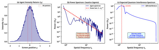
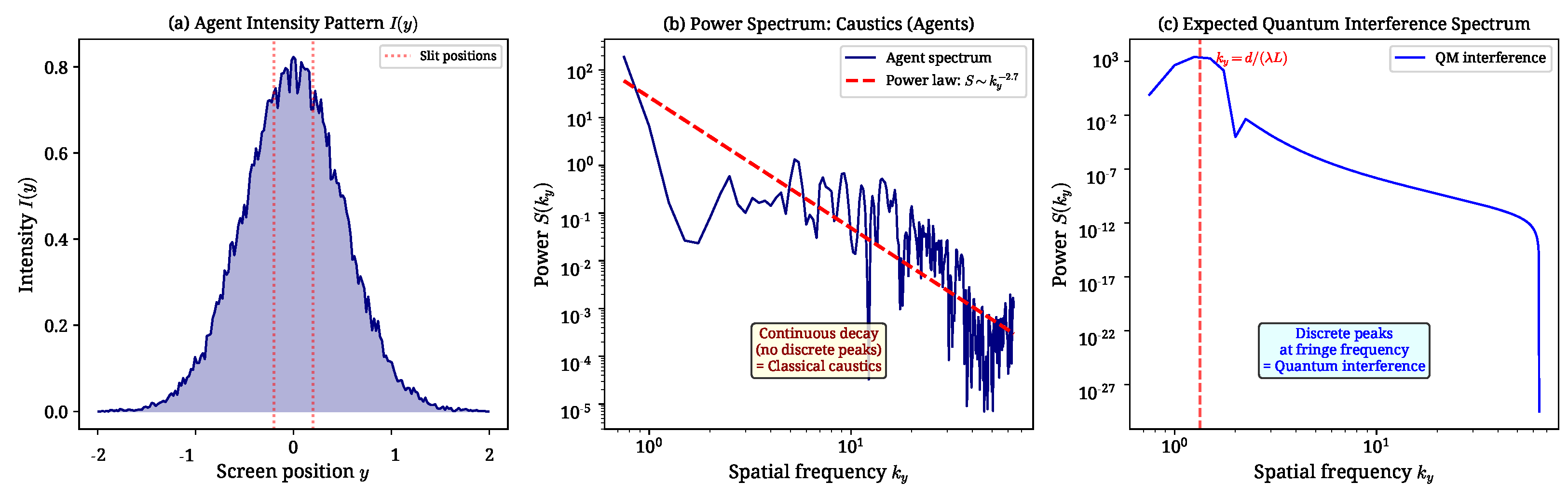
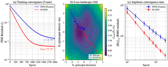
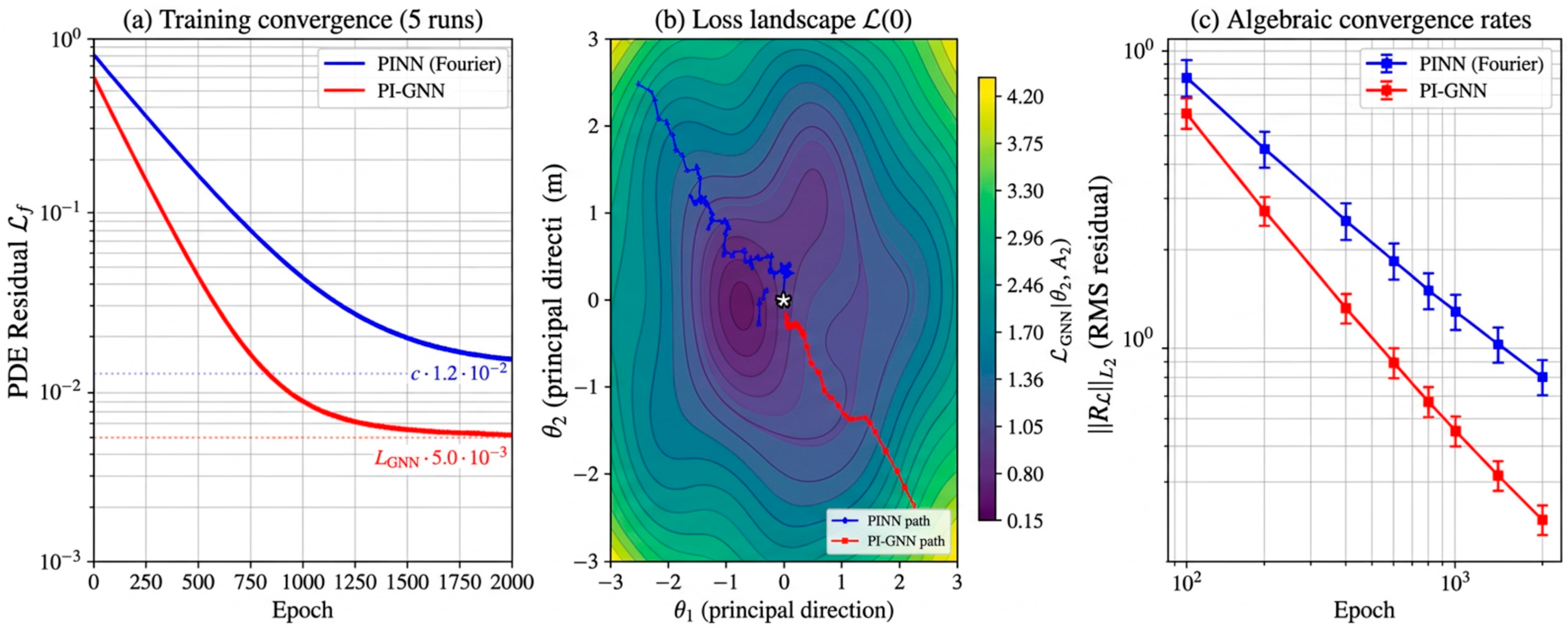
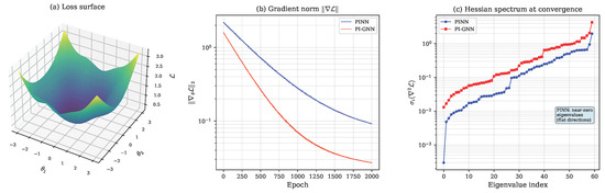
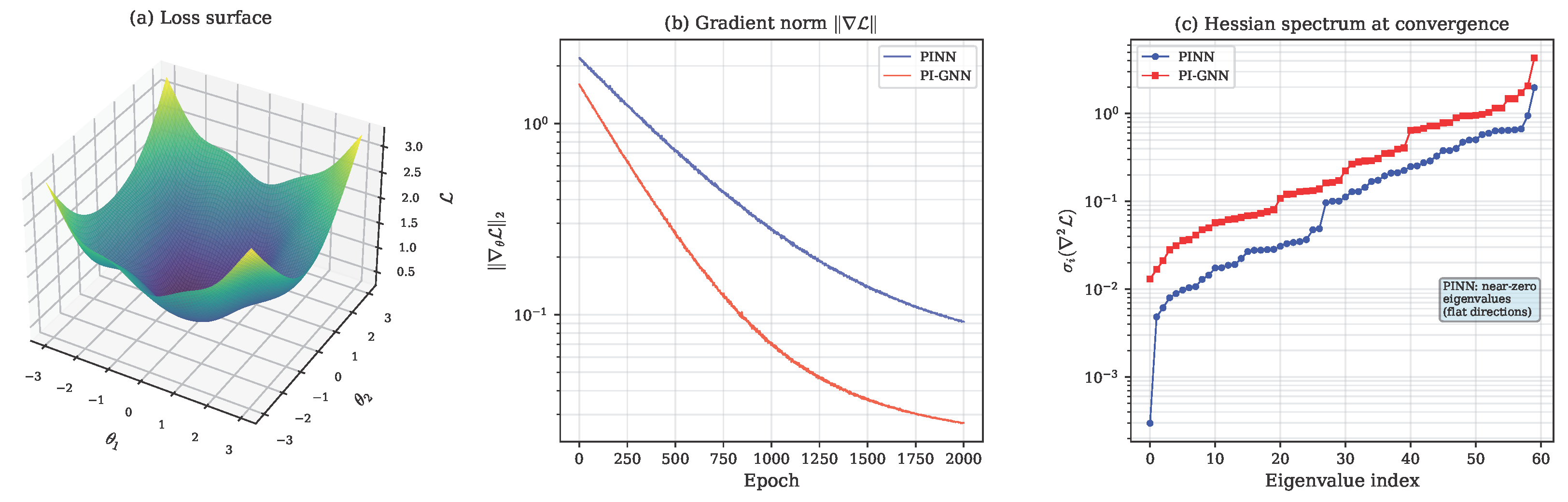
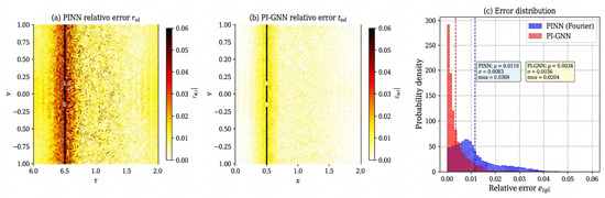
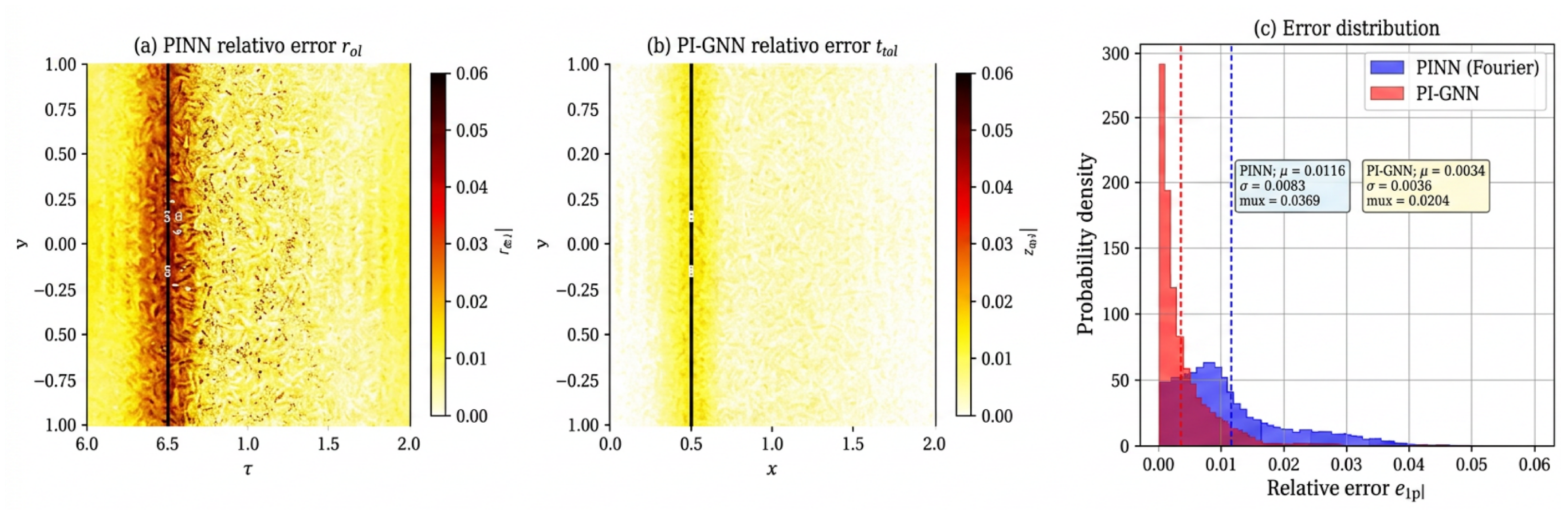
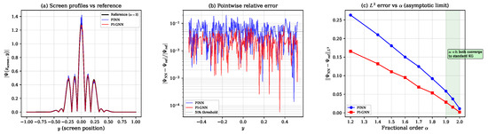
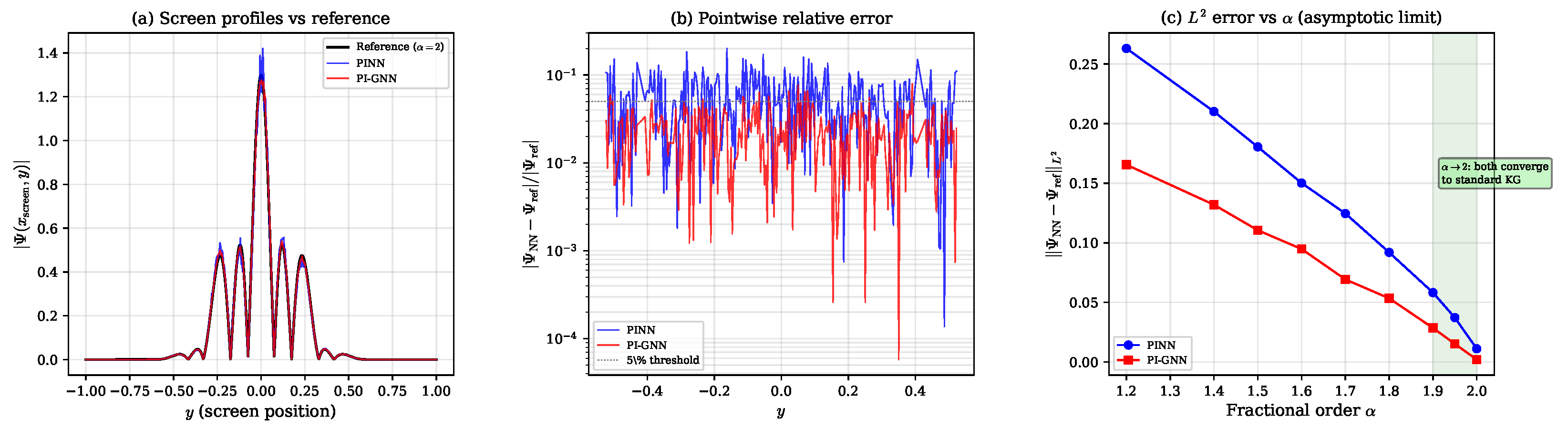
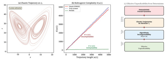
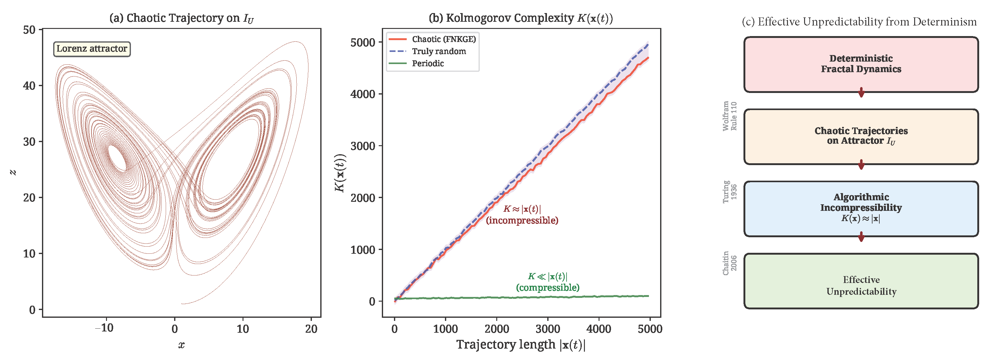
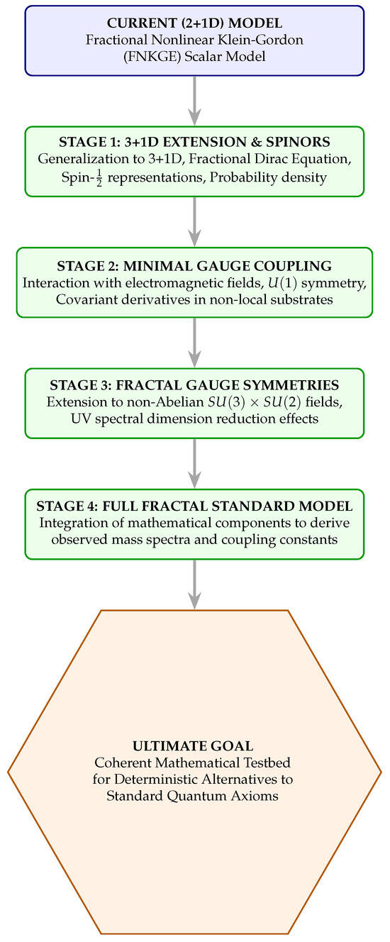
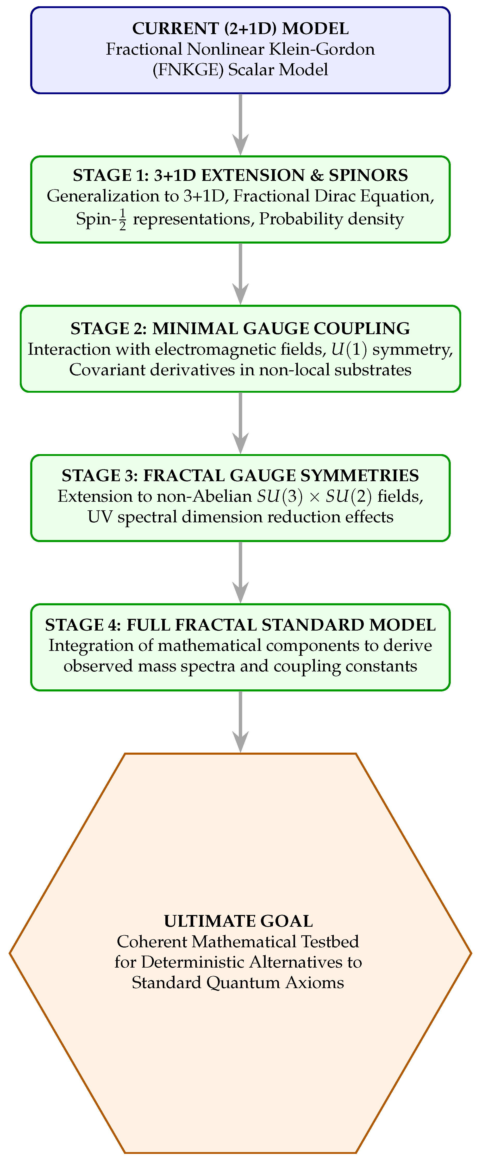

Disclaimer/Publisher’s Note: The statements, opinions and data contained in all publications are solely those of the individual author(s) and contributor(s) and not of MDPI and/or the editor(s). MDPI and/or the editor(s) disclaim responsibility for any injury to people or property resulting from any ideas, methods, instructions or products referred to in the content. |
© 2026 by the authors. Licensee MDPI, Basel, Switzerland. This article is an open access article distributed under the terms and conditions of the Creative Commons Attribution (CC BY) license.