Employing the Double Natural Generalized Laplace Transform to Solve Singular Boussinesq Equations in Two Dimensions

Abstract

The double natural generalized Laplace transform decomposition method (DNGLTDM) is proposed as a new approach for solving singular linear and non-linear two-dimensional Boussinesq equations involving fractional partial derivatives. This method combines the decomposition technique with the double natural generalized Laplace transform to construct solutions in the form of rapidly convergent infinite series that approximate the exact solutions. The paper presents a detailed study of the fundamental properties of the transform, including the convolution theorem, the periodicity theorem, the treatment of partial derivatives with non-constant coefficients, and partial fractional derivatives. In addition, the convergence of the obtained series solutions and the associated error analysis are thoroughly investigated. Finally, two illustrative examples are provided to demonstrate the accuracy and effectiveness of the DNGLTDM, one of which considers a problem of partial fractional order.

1. Introduction

In physics and engineering, linear and non-linear partial differential equations (PDEs) are very important for modeling a wide range of events. The two-dimensional Boussinesq equation stands out among these equations. It accurately describes a range of mathematical, physical, and technological processes, such as simulating water flow in unconfined aquifers. Boussinesq-type equations also come up in a lot of different situations, such as one-dimensional non-linear lattice dynamics [1] and shallow-water waves [2,3]. The authors of [4] examined the Allen–Cahn equation utilizing the Caputo–Hadamard fractional derivative in time through a numerical algorithm. The existence and uniqueness of solutions to Caputo–Hadamard differential equations with delay and non-local conditions are examined in [5]. Many analytical methods have been created over the past few decades to find clear and correct answers to these kinds of problems. For instance, the q-homotopy analysis transform method was used to solve the Schrödinger–Boussinesq equation [6]. The authors of [7,8,9,10] examined Boussinesq equations using the modified decomposition method, whereas analytical solutions to Boussinesq-like equations were subsequently explored through the homotopy perturbation method [11]. Recently, the non-linear fractional Boussinesq equation with the Caputo fractional derivative has been examined using the modified double Laplace decomposition method (MDLDM) to determine the general approximate solution in [12]. The authors of [13] employed two numerical techniques, namely the variational iteration transform method (VITM) and the Adomian decomposition method (ADM), to solve the second- and fourth-order fractional Boussinesq equations. Numerical methods have also been extensively utilized. The Boussinesq–Burger equations were examined using the optimal homotopy asymptotic method [14], while the generalized Boussinesq equation was investigated through the homotopy analysis method [15]. The Laplace–Adomian decomposition method yielded both approximate and analytical solutions for the Boussinesq–Burger equation [16]. In [17], the authors developed precise traveling wave solutions for the (2+1)-dimensional Boussinesq equation using the repeated homogeneous balance method. Recently, integral transform methods have garnered heightened interest. The natural transform was integrated with the natural decomposition method to address coupled systems of non-linear partial differential equations [18]. Recently, the double natural transform was used to solve telegraph, wave, and partial integro-differential equations [19].

Based on these advancements, the current study introduces a methodology for addressing the singular two-dimensional Boussinesq equation through the double natural generalized Laplace transform decomposition method (DNGLTDM). This analytical method shows that (DNGLTDM) works well for finding solutions to non-linear differential equations. This method is broader than the triple Sumudu transform, the triple Laplace transform, and the double Laplace–Yang transform. We can learn some things from it, and all of these things can be learned from our method, the double natural generalized Laplace transform. To be thorough, let us go over the definitions of the natural transform (NT) and the generalized Laplace transform (GLT) again.

In the following, we provide some fundamental definitions:

Definition 1.

Consider the set of functions

$$A=\left\{\begin{array}{c}f\left(x\right):\exists M,{\tau }_1,{\tau }_2>0\mathit{such}\mathit{that}\\ \left|f\left(x\right)\right|<M{e}^{{\displaystyle \frac{\left|x\right|}{{\tau }_j}}},x\in {(-1)}^j\times [0,\infty ),j=1,2\end{array}\right\}.$$

For functions in A, the natural transform (NT) is defined as

$${\mathbf{N}}_x^{+}\left[f\left(x\right)\right]=R(p;u)={\displaystyle \frac{1}{u}}{\int }_0^{\infty }{e}^{-{\displaystyle \frac{p}{u}}x}f\left(x\right)dx,$$

(1)

where u and p are complex variables with $\mathrm{Re}\left(p\right)>0$ and $\mathrm{Re}\left(u\right)>0$.

For further details on the natural transform, we refer the reader to [20,21].

Definition 2

([22]). Let $f\left(\theta \right)$ be an integrable function for all $\theta \ge 0$. The generalized Laplace transform $G_{\alpha }$ of $f\left(\theta \right)$ is defined as

$$F\left(s\right)=G_{\alpha }\left(f\right)=s^{\alpha }{\int }_0^{\infty }f\left(\theta \right)e^{-{\displaystyle \frac{\theta }{s}}}d\theta ,$$

(2)

for $s\in \mathbb{C}$ and $\alpha \in \mathbb{Z}$.

Definition 3

([23]). The double natural transform (DNT) is defined by

$$\begin{array}{ccc}\hfill {\mathbf{N}}_{x,y}^{+}\left[f(x,y)\right]& =& F(p;u,q;v)\hfill \\ & =& {\displaystyle \frac{1}{uv}}{\int }_0^{\infty }{\int }_0^{\infty }{e}^{-{\displaystyle \frac{p}{u}}x-{\displaystyle \frac{q}{v}}y}f(x,y)dydx,\hfill \\ \hfill \mathrm{Re}\left(p\right),\mathrm{Re}\left(q\right)& >& 0,\mathrm{Re}\left(u\right)>0,\mathrm{Re}\left(v\right)>0.\hfill \end{array}$$

(3)

where ${\mathbf{N}}_{x,y}^{+}$ denotes the DNT. The inverse double natural transform (IDNGLT) is given by

$$\begin{array}{cc}\hfill {\mathbf{N}}_{p;u,q;v}^{-1}& \left(F(p;u,q;v)\right)\hfill \\ & =f(x,y)\hfill \\ & ={\displaystyle \frac{1}{{\left(2\pi i\right)}^2}}{\int }_{\beta -i\infty }^{\beta +i\infty }{\int }_{\xi -i\infty }^{\xi +i\infty }{e}^{{\displaystyle \frac{p}{u}}x+{\displaystyle \frac{q}{v}}y}F(p;u,q;v)dqdp.\hfill \end{array}$$

Definition 4.

The left-side Caputo fractional derivative of f, $f\in C_{-1}^m,$ and $m\in \mathbb{N}\cup \left\{0\right\}$ is described in [24] as

$$D_{*}^{\delta }f\left(\theta \right)={\displaystyle \frac{{\partial }^{\delta }f\left(\theta \right)}{\partial {\theta }^{\delta }}}=\left\{\begin{array}{c}{I}^{n-\delta }\left[{\displaystyle \frac{{\partial }^{n}f\left(\theta \right)}{\partial {\theta }^n}}\right],n-1<\delta <n,n\in \mathbb{N}\hfill \\ {\displaystyle \frac{{\partial }^{n}f\left(\theta \right)}{\partial {\theta }^n}},\delta =n\hfill \end{array},\right.$$

Definition 5

([25]). The partial fractional integrals and Caputo derivatives of a function $f\left(x,\theta \right)$, where $\left(x,\theta \right)\in {\mathbb{R}}^{+}\times {\mathbb{R}}^{+}$ are granted by

$$D_{\theta }^{\delta }f\left(x,\theta \right)={\displaystyle \frac{1}{\Gamma \left(n-\delta \right)}}{\int }_0^{\theta }{\left(\theta -\lambda \right)}^{n-\delta -1}{\displaystyle \frac{{\partial }^n}{\partial {\lambda }^n}}f\left(x,\lambda \right)d\lambda ,$$

(4)

where $n-1<\delta \le n,$ $0<$ $\delta .$

In the subsequent sections, we present the main results of this work.

2. Main Results of the Double Natural Generalized Laplace Transform (DNGLT)

In this section, we discuss the basic ideas and properties of the double natural generalized Laplace transform (DNGLT).

If we put Definitions 2 and 3 together, we get a new one called the double natural generalized Laplace transform (DNGLT), as follows:

Definition 6.

The double natural generalized Laplace transform (DNGLT) is defined by

$$\begin{array}{ccc}\hfill {\mathbf{N}}_{x,y}^{+}{G}_{\alpha }\left[f(x,y,\theta )\right]& =& F(p;u,q;v,s)\hfill \\ & =& {\displaystyle \frac{s^{\alpha }}{uv}}{\int }_0^{\infty }{\int }_0^{\infty }{\int }_0^{\infty }{e}^{-{\displaystyle \frac{p}{u}}x-{\displaystyle \frac{q}{v}}y-{\displaystyle \frac{1}{s}}\theta }f(x,y,\theta )d\theta dydx,\hfill \\ \hfill \mathrm{Re}\left(s\right),\mathrm{Re}\left(p\right),\mathrm{Re}\left(q\right)& >& 0,\mathrm{Re}\left(u\right)>0,\mathrm{Re}\left(v\right)>0.\hfill \end{array}$$

(5)

where ${\mathbf{N}}_{x,y}^{+}{G}_{\alpha }$ denotes the DNGLT. The inverse double natural generalized Laplace transform (IDNGLT) is given by

$$\begin{array}{cc}\hfill {\mathbf{N}}_{p;u,q;v}^{-1}{G}_s^{-1}& \left(F(p;u,q;v,s)\right)\hfill \\ & =f(x,y,\theta )\hfill \\ & ={\displaystyle \frac{1}{{\left(2\pi i\right)}^3}}{\int }_{\lambda -i\infty }^{\lambda +i\infty }{\int }_{\beta -i\infty }^{\beta +i\infty }{\int }_{\xi -i\infty }^{\xi +i\infty }{e}^{{\displaystyle \frac{p}{u}}x+{\displaystyle \frac{q}{v}}y+{\displaystyle \frac{1}{s}}\theta }F(p;u,q;v,s)dsdqdp.\hfill \end{array}$$

In this study, we use $N_2^{-1}$ instead of $N_{p;u,q;v}^{-1}$.

Remark 1.

From the definition of the DNGLT, several well-known transforms can be obtained as special cases:

1. 

Setting $\alpha =-1$, $p=1$, and $q=1$, we obtain the triple Sumudu transform:

$${\mathbf{S}}_x{\mathbf{S}}_y{S}_{\theta }\left[f(x,y,\theta )\right]=F(u,v,s)={\displaystyle \frac{1}{uvs}}{\int }_0^{\infty }{\int }_0^{\infty }{\int }_0^{\infty }{e}^{-{\displaystyle \frac{1}{u}}x-{\displaystyle \frac{1}{v}}y-{\displaystyle \frac{1}{s}}\theta }f(x,y,\theta )d\theta dydx.$$

2. 

Setting $\alpha =0$, $u=1$, $v=1$, and $s={\displaystyle \frac{1}{s}}$, we obtain the triple Laplace transform:

$$L_x{L}_y{L}_{\theta }\left[f(x,y,\theta )\right]=F(p,q,s)={\int }_0^{\infty }{\int }_0^{\infty }{\int }_0^{\infty }{e}^{-px-qy-s\theta }f(x,y,\theta )d\theta dydx.$$

3. 

Setting $\alpha =0$, $u=1$, $v=1$, and $s=\omega$, we obtain the double Laplace–Yang transform:

$$L_x{L}_{y}Y\left[f(x,y,\theta )\right]=F(p,q,\omega )={\int }_0^{\infty }{\int }_0^{\infty }{\int }_0^{\infty }{e}^{-px-qy-{\displaystyle \frac{1}{\omega }}\theta }f(x,y,\theta )d\theta dydx.$$

The following examples illustrate the application of the DNGLT:

Example 1.

The DNGLT of the function $f(x,y,\theta )=e^{ax+by+c\theta }$ is given by

$$F(p;u,q;v,s)={\mathbf{N}}_{x,y}^{+}{G}_{\alpha }\left[e^{ax+by+c\theta }\right]={\displaystyle \frac{1}{(p-au)}}{\displaystyle \frac{1}{(q-bv)}}{\displaystyle \frac{s^{\alpha +1}}{(1-bs)}}.$$

Example 2.

For $f(x,y,\theta )={\left(xy\theta \right)}^n$, the DNGLT is

$${\mathbf{N}}_{x,y}^{+}{G}_{\alpha }\left[{\left(xy\theta \right)}^n\right]={\displaystyle \frac{{(n!)}^3{u}^n{v}^n{s}^{n+\alpha +1}}{p^{n+1}{q}^{n+1}}},$$

where n is a positive integer.

If $a>-1,b>-1,c>-1$ are real numbers, then

$${\mathbf{N}}_{x,y}^{+}{G}_{\alpha }\left[x^a{y}^b{\theta }^c\right]={\displaystyle \frac{u^a{v}^b\Gamma (a+1)\Gamma (b+1)\Gamma (c+1)s^{\alpha +c+1}}{p^{a+1}{q}^{b+1}}}.$$

It follows directly from the definition of the DNGLT that

$$\begin{array}{ccc}\hfill {\mathbf{N}}_{x,y}^{+}{G}_{\alpha }\left[x^a{y}^b{\theta }^c\right]& =& {\displaystyle \frac{s^{\alpha }}{uv}}{\int }_0^{\infty }{\int }_0^{\infty }{\int }_0^{\infty }{e}^{-{\displaystyle \frac{p}{u}}x-{\displaystyle \frac{q}{v}}y-{\displaystyle \frac{1}{s}}\theta }{x}^a{y}^b{\theta }^{c}d\theta dydx\hfill \\ & =& {\displaystyle \frac{1}{uv}}{\int }_0^{\infty }{\int }_0^{\infty }{e}^{-{\displaystyle \frac{p}{u}}x-{\displaystyle \frac{q}{v}}y}{x}^a{y}^b\left(s^{\alpha }{\int }_0^{\infty }{e}^{-{\displaystyle \frac{1}{s}}\theta }{\theta }^{c}d\theta \right)dydx.\hfill \end{array}$$

By substituting $\frac{p}{u}x=r$, $\frac{q}{v}y=h$, and $\frac{1}{s}\theta =k$, we obtain

$$\begin{array}{ccc}\hfill {\mathbf{N}}_{x,y}^{+}{G}_{\alpha }\left[x^a{y}^b{\theta }^c\right]& =& {\displaystyle \frac{u^a}{p^{a+1}}}{\displaystyle \frac{v^b}{q^{b+1}}}{s}^{\alpha +c+1}{\int }_0^{\infty }{\int }_0^{\infty }{\int }_0^{\infty }{r}^a{h}^b{k}^c{e}^{-r}{e}^{-h}{e}^{-k}drdhdk\hfill \\ & =& {\displaystyle \frac{u^a{v}^b\Gamma (a+1)\Gamma (b+1)\Gamma (c+1)s^{\alpha +c+1}}{p^{a+1}{q}^{b+1}}}.\hfill \end{array}$$

Here, the Gamma functions of $a, b,$ and c are defined by the uniformly convergent integrals

$$\Gamma \left(x\right)={\int }_0^{\infty }{e}^{-r}{r}^{x-1}dr,$$

2.1. Existence Condition for the (DNGLT)

A function $f(x,y,\theta )$ is said to be of exponential order $(\alpha ,\beta ,\gamma )$ as $x,y,\theta \to \infty$ if there exist positive constants $\Omega ,X,Y,\Lambda$ such that

$$\left|f(x,y,\theta )\right|\le \Omega e^{\alpha x+\beta y+\gamma \theta },\forall x>X,y>Y,\theta >\Lambda .$$

(6)

Equivalently, this means

$$f(x,y,\theta )=O\left(e^{\alpha x+\beta y+\gamma \theta }\right)\mathrm{as}x,y,\theta \to \infty ,$$

or, in limit form,

$$\underset{\begin{array}{c}x\to \infty \\ y\to \infty \\ \theta \to \infty \end{array}}{lim}{e}^{-{\displaystyle \frac{\mu }{u}}x-{\displaystyle \frac{\lambda }{v}}y-{\displaystyle \frac{1}{s}}\theta }\left|f(x,y,\theta )\right|=\Omega \underset{\begin{array}{c}x\to \infty \\ y\to \infty \\ \theta \to \infty \end{array}}{lim}{e}^{-\left({\displaystyle \frac{\mu }{u}}-\alpha \right)x}{e}^{-\left({\displaystyle \frac{\lambda }{v}}-\beta \right)y}{e}^{-\left({\displaystyle \frac{1}{s}}-\gamma \right)\theta }=0,$$

whenever $\frac{\mu }{u}>\alpha$, $\frac{\lambda }{v}>\beta$, and $\frac{1}{s}>\gamma$. Such a function $f(x,y,\theta )$ is simply called an exponential order as $x,y,\theta \to \infty$. Clearly, this does not grow faster than $\Omega e^{\alpha x+\beta y+\gamma \theta }$.

We use the same method as in Theorem 1 in [26] to prove the next theorem of existence conditions for the (DNGLT).

Theorem 1.

Let $f(x,y,\theta )$ be a continuous function on $(0,X)\times (0,Y)\times (0,\Lambda )$ and of exponential order $e^{\alpha x+\beta y+\gamma \theta }$. Then the DNGLT of $f(x,y,\theta )$, denoted by $F(p;u,q;v,s)$, exists for all $\mathrm{Re}\left({\displaystyle \frac{p}{u}}\right)>{\displaystyle \frac{\mu }{u}},\mathrm{Re}\left({\displaystyle \frac{q}{v}}\right)>{\displaystyle \frac{\lambda }{v}},$ and $\mathrm{Re}\left({\displaystyle \frac{1}{s}}\right)>{\displaystyle \frac{1}{\nu }},$ with $u\ne 0$ and $\nu \ne 0$.

Proof. 

By applying the definition of the DNGLT to $f(x,y,\theta )$, we have

$$\begin{array}{ccc}\hfill \left|F(p;u,q;v,s)\right|& =& \left|{\displaystyle \frac{s^{\alpha }}{uv}}{\int }_0^{\infty }{\int }_0^{\infty }{\int }_0^{\infty }{e}^{-{\displaystyle \frac{p}{u}}x-{\displaystyle \frac{q}{v}}y-{\displaystyle \frac{1}{s}}\theta }f(x,y,\theta )d\theta dydx\right|\hfill \\ & \le & \Omega \left|{\displaystyle \frac{s^{\alpha }}{uv}}{\int }_0^{\infty }{\int }_0^{\infty }{\int }_0^{\infty }{e}^{-({\displaystyle \frac{p}{u}}-\alpha )x-({\displaystyle \frac{q}{v}}-\beta )y-({\displaystyle \frac{1}{s}}-\gamma )\theta }d\theta dydx\right|\hfill \\ & =& {\displaystyle \frac{\Omega s^{\alpha +1}}{(p-\alpha u)(q-\beta v)(1-\gamma s)}}.\hfill \end{array}$$

(7)

It follows from Equation (7) that

$$\underset{\begin{array}{c}p\to \infty \\ q\to \infty \\ \frac{1}{s}\to \infty \end{array}}{lim}\left|F(p;u,q;v,s)\right|=0,\mathrm{or}\mathrm{equivalently},\underset{\begin{array}{c}p\to \infty \\ q\to \infty \\ \frac{1}{s}\to \infty \end{array}}{lim}F(p;u,q;v,s)=0.$$

Hence, the DNGLT exists under the stated conditions. □

Theorem 2.

Assume that the (DNGLT) of the function $f(x,y,\theta )$ exists and $f(x,y,\theta )$ is a periodic function of periods $K,H$, and E where $f(x+k,y+H,\theta +E)=f(x,y,\theta ),$ $\forall \left(x,y,\theta \right)$. Then

$${\mathbf{N}}_{x,y}^{+}{G}_{\alpha }\left[f\left(x,y,\theta \right)\right]={\displaystyle \frac{\frac{s^{\alpha }}{uv}{\int }_0^k{\int }_0^H{\int }_0^E{e}^{-\frac{p}{u}x-\frac{q}{v}y-\frac{1}{s}\theta }f\left(x,y,\theta \right)d\theta dydx}{\left(1-e^{-\frac{p}{u}K-\frac{q}{v}H-\frac{1}{s}E}\right)}}$$

Proof. 

By using the definition of the (DNGLT), we have

$$\begin{array}{ccc}\hfill {\mathbf{N}}_{x,y}^{+}{G}_{\alpha }\left[f\left(x,y,\theta \right)\right]& =& {\displaystyle \frac{s^{\alpha }}{uv}}{\int }_0^{\infty }{\int }_0^{\infty }{\int }_0^{\infty }{e}^{-{\displaystyle \frac{p}{u}}x-{\displaystyle \frac{q}{v}}y-{\displaystyle \frac{1}{s}}\theta }f\left(x,y,\theta \right)d\theta dydx\hfill \end{array}$$

Utilizing the following, let $x=k+\rho$, $y=H+\tau$, and $\theta =E+\sigma$, the above integral, become

$$\begin{array}{cc}\hfill {\mathbf{N}}_{x,y}^{+}{G}_{\alpha }& \left[f\left(x,y,\theta \right)\right]\hfill \\ & ={\displaystyle \frac{s^{\alpha }}{uv}}{\int }_0^k{\int }_0^H{\int }_0^E{e}^{-{\displaystyle \frac{p}{u}}x-{\displaystyle \frac{q}{v}}y-{\displaystyle \frac{1}{s}}\theta }f\left(x,y,\theta \right)d\theta dydx\hfill \\ \hfill & +{\displaystyle \frac{s^{\alpha }}{uv}}{e}^{-{\displaystyle \frac{p}{u}}k-{\displaystyle \frac{q}{v}}H-{\displaystyle \frac{1}{s}}E}{\int }_0^{\infty }{\int }_0^{\infty }{\int }_0^{\infty }{e}^{-{\displaystyle \frac{p}{u}}\rho -{\displaystyle \frac{q}{v}}\tau -{\displaystyle \frac{1}{s}}\sigma }f\left(k+\rho ,H+\tau ,E+\sigma \right)d\sigma d\tau d\rho .\hfill \end{array}$$

By utilizing the formula $f\left(k+\rho ,H+\tau ,E+\sigma \right)=f(x,y,\theta ),$ hence the over equation become

$$\begin{array}{ccc}\hfill {\mathbf{N}}_{x,y}^{+}{G}_{\alpha }\left[f\left(x,y,\theta \right)\right]& =& {\displaystyle \frac{s^{\alpha }}{uv}}{\int }_0^k{\int }_0^H{\int }_0^E{e}^{-{\displaystyle \frac{p}{u}}x-{\displaystyle \frac{q}{v}}y-{\displaystyle \frac{1}{s}}\theta }f\left(x,y,\theta \right)d\theta dydx\hfill \\ & & +{\displaystyle \frac{s^{\alpha }}{uv}}{e}^{-{\displaystyle \frac{p}{u}}k-{\displaystyle \frac{q}{v}}H-{\displaystyle \frac{1}{s}}E}{\int }_0^{\infty }{\int }_0^{\infty }{\int }_0^{\infty }{e}^{-{\displaystyle \frac{p}{u}}\rho -{\displaystyle \frac{q}{v}}\tau -{\displaystyle \frac{1}{s}}\sigma }f\left(\rho ,\tau ,\sigma \right)d\sigma d\tau d\rho ,\hfill \end{array}$$

thus

$$\begin{array}{ccc}\hfill {\mathbf{N}}_{x,y}^{+}{G}_{\alpha }\left[f\left(x,y,\theta \right)\right]& =& {\displaystyle \frac{s^{\alpha }}{uv}}{\int }_0^k{\int }_0^H{\int }_0^E{e}^{-{\displaystyle \frac{p}{u}}x-{\displaystyle \frac{q}{v}}y-{\displaystyle \frac{1}{s}}\theta }f\left(x,y,\theta \right)d\theta dydx\hfill \\ & & +e^{-{\displaystyle \frac{p}{u}}k-{\displaystyle \frac{q}{v}}H-{\displaystyle \frac{1}{s}}E}{\mathbf{N}}_{x,y}^{+}{G}_{\theta }\left[f\left(x,y,\theta \right)\right],\hfill \end{array}$$

accordingly

$${\mathbf{N}}_{x,y}^{+}{G}_{\alpha }\left[f\left(x,y,\theta \right)\right]={\displaystyle \frac{\frac{s^{\alpha }}{uv}{\int }_0^k{\int }_0^H{\int }_0^E{e}^{-\frac{p}{u}x-\frac{q}{v}y-\frac{1}{s}\theta }f\left(x,y,\theta \right)d\theta dydx}{\left(1-e^{-\frac{p}{u}k-\frac{q}{v}H-\frac{1}{s}E}\right)}}.$$

□

Theorem 3.

If DNGLT of the function $f\left(x,y,\theta \right)$ is given by $F\left(p;u,q;v,s\right)$ then

$$\begin{array}{ccc}& & {\mathbf{N}}_{x,y}^{+}{G}_{\alpha }\left[f\left(x-\zeta ,y-\eta ,\theta -\lambda \right)H\left(x-\zeta ,y-\eta ,\theta -\lambda \right)\right]\hfill \\ & =& e^{-{\displaystyle \frac{p}{u}}\zeta -{\displaystyle \frac{q}{v}}\eta -{\displaystyle \frac{1}{s}}\lambda }{\displaystyle \frac{s^{\alpha }}{uv}}\underset{0}{\overset{\infty }{\int }}\underset{0}{\overset{\infty }{\int }}\underset{0}{\overset{\infty }{\int }}{e}^{-{\displaystyle \frac{p}{u}}\mu -{\displaystyle \frac{q}{v}}\varpi -{\displaystyle \frac{1}{s}}\tau }f\left(\mu ,\varpi ,\tau \right)d\tau d\varpi d\mu \hfill \end{array}$$

where $H\left(x,y,\theta \right)$ is the Heaviside unit step function defined by

$H\left(x-a,y-b,\theta -c\right)=1$ at $x>a,$ $y>b,$ $\theta >c$, and $H\left(x-a,y-b,\theta -c\right)=0$ at

$x<a,$$y<b,$$\theta <c.$

Proof. 

By the definition of DNGLT, we have

$$\begin{array}{ccc}& & {\mathbf{N}}_{x,y}^{+}{G}_{\alpha }\left[f\left(x-\zeta ,y-\eta ,\theta -\lambda \right)H\left(x-\zeta ,y-\eta ,\theta -\lambda \right)\right]\hfill \\ & =& {\displaystyle \frac{s^{\alpha }}{uv}}\underset{0}{\overset{\infty }{\int }}\underset{0}{\overset{\infty }{\int }}\underset{0}{\overset{\infty }{\int }}{e}^{-{\displaystyle \frac{p}{u}}x-{\displaystyle \frac{q}{v}}y-{\displaystyle \frac{1}{s}}\theta }f\left(x-\zeta ,y-\eta ,\theta -\lambda \right)H\left(x-\zeta ,y-\eta ,\theta -\lambda \right)d\theta dydx\hfill \\ & =& {\displaystyle \frac{s^{\alpha }}{uv}}\underset{\zeta }{\overset{\infty }{\int }}\underset{\eta }{\overset{\infty }{\int }}\underset{\lambda }{\overset{\infty }{\int }}{e}^{-{\displaystyle \frac{p}{u}}x-{\displaystyle \frac{q}{v}}y-{\displaystyle \frac{1}{s}}\theta }f\left(x-\zeta ,y-\eta ,\theta -\lambda \right)d\theta dydx,\hfill \end{array}$$

by putting $x-\zeta =\mu ,$ $y-\eta =\varpi ,$ $\theta -\lambda =\tau$

$$\begin{array}{ccc}& & {\mathbf{N}}_{x,y}^{+}{G}_{\alpha }\left[f\left(x-\zeta ,y-\eta ,\theta -\lambda \right)H\left(x-\zeta ,y-\eta ,\theta -\lambda \right)\right]\hfill \\ & =& e^{-{\displaystyle \frac{p}{u}}\zeta -{\displaystyle \frac{q}{v}}\eta -{\displaystyle \frac{1}{s}}\lambda }{\displaystyle \frac{s^{\alpha }}{uv}}\underset{0}{\overset{\infty }{\int }}\underset{0}{\overset{\infty }{\int }}\underset{0}{\overset{\infty }{\int }}{e}^{-{\displaystyle \frac{p}{u}}\mu -{\displaystyle \frac{q}{v}}\varpi -{\displaystyle \frac{1}{s}}\tau }f\left(\mu ,\varpi ,\tau \right)d\tau d\varpi d\mu ,\hfill \end{array}$$

□

2.2. The Double Natural Transform of the Convolution Product

Theorem 4.

Assume that the (DNGLT) of the functions $f(x,y,\theta )$ and $g(x,y,\theta )$ exist. Then the (DNGLT) of the triple convolution of the $f(x,y,\theta )$ and $g(x,y,\theta )$,

$$\left(f\ast \ast \ast g\right)\left(x,y,\theta \right)={\int }_0^x{\int }_0^y{\int }_0^{\theta }f\left(\zeta ,\eta ,\kappa \right)g\left(x-\zeta ,y-\eta ,\theta -\kappa \right)d\zeta d\eta d\kappa ,$$

(8)

is identified by

$${\mathbf{N}}_{x,y}^{+}{G}_{\theta }\left[f\ast \ast \ast g\left(x,y,\theta \right)\right]={\displaystyle \frac{uv}{s^{\alpha }}}F\left(p;u,q;v,s\right)G\left(p;u,q;v,s\right),$$

(9)

where $F\left(p;u,q;v,s\right)$ and $G\left(p;u,q;v,s\right)$ are the (DNGLT) of the functions $f\left(x,y,\theta \right)$ and $g\left(x,y,\theta \right)$ respectively.

Proof. 

Exploiting the definition of the (DNGLT) and triple convolution grants that

$$\begin{array}{cc}\hfill {\mathbf{N}}_{x,y}^{+}{G}_{\alpha }& \left[f\left(x,y,\theta \right)\ast \ast \ast g\left(x,y,\theta \right)\right]\hfill \\ \hfill & ={\displaystyle \frac{s^{\alpha }}{uv}}{\int }_0^{\infty }{\int }_0^{\infty }{\int }_0^{\infty }{e}^{-{\displaystyle \frac{p}{u}}x-{\displaystyle \frac{q}{v}}y-{\displaystyle \frac{1}{s}}\theta }f\left(x,y,\theta \right)\ast \ast \ast g\left(x,y,\theta \right)d\theta dydx\hfill \\ \hfill & ={\displaystyle \frac{s^{\alpha }}{uv}}{\int }_0^{\infty }{\int }_0^{\infty }{\int }_0^{\infty }{e}^{-{\displaystyle \frac{p}{u}}x-{\displaystyle \frac{q}{v}}y-{\displaystyle \frac{1}{s}}\theta }\hfill \\ & \left({\int }_0^x{\int }_0^y{\int }_0^{\theta }f\left(\zeta ,\eta ,\kappa \right)g\left(x-\zeta ,y-\eta ,\theta -\kappa \right)d\zeta d\eta d\kappa \right)d\theta dydx.\hfill \end{array}$$

using the Heaviside unit step function, which is defined in Theorem 3. Set $\gamma =x-\zeta ,\xi =y-\eta$ and $\delta =\theta -\kappa$ and extend the higher boundaries of integrals to $x\to \infty$, $y\to \infty$, $\theta \to \infty$; thus, we have

$$\begin{array}{cc}\hfill {\mathbf{N}}_{x,y}^{+}{G}_{\alpha }& \left[f\left(x,y,\theta \right)\ast \ast \ast g\left(x,y,\theta \right)\right]\hfill \\ \hfill & ={\displaystyle \frac{s^{\alpha }}{uv}}{\int }_0^{\infty }{\int }_0^{\infty }{\int }_0^{\infty }{e}^{-{\displaystyle \frac{p}{u}}x-{\displaystyle \frac{q}{v}}y-{\displaystyle \frac{1}{s}}\theta }f\left(\zeta ,\eta ,\kappa \right)\hfill \\ & \left({\int }_{-\gamma }^{\infty }{\int }_{-\delta }^{\infty }{\int }_{-\xi }^{\infty }{e}^{-{\displaystyle \frac{p}{u}}\gamma -{\displaystyle \frac{q}{v}}\xi -{\displaystyle \frac{1}{s}}\delta }g\left(\gamma ,\xi ,\delta \right)d\gamma d\xi d\delta \right)d\zeta d\eta d\kappa ,\hfill \end{array}$$

where the functions $f\left(x,y,\theta \right),$ $g\left(x,y,\theta \right)$ are determined at $x>0, y>0,$ and $\theta >0.$ Consequently, $f\left(x,y,\theta \right),$ $g\left(x,y,\theta \right)$ are zero at $x<0$, $y<0,$ and $\theta <0,$ thus

$$\begin{array}{cc}\hfill {\mathbf{N}}_{x,y}^{+}{G}_{\alpha }& \left[f\left(x,y,\theta \right)\ast \ast \ast g\left(x,y,\theta \right)\right]\hfill \\ \hfill & ={\displaystyle \frac{uv}{s^{\alpha }}}{\displaystyle \frac{s^{\alpha }}{uv}}{\int }_0^{\infty }{\int }_0^{\infty }{\int }_0^{\infty }{e}^{-{\displaystyle \frac{p}{u}}x-{\displaystyle \frac{q}{v}}y-{\displaystyle \frac{1}{s}}\theta }f\left(\zeta ,\eta ,\kappa \right)\hfill \\ & \left({\displaystyle \frac{s^{\alpha }}{uv}}{\int }_0^{\infty }{\int }_0^{\infty }{\int }_0^{\infty }{e}^{-{\displaystyle \frac{p}{u}}\gamma -{\displaystyle \frac{q}{v}}\xi -{\displaystyle \frac{1}{s}}\delta }g\left(\gamma ,\xi ,\delta \right)d\gamma d\xi d\delta \right)d\zeta d\eta d\kappa .\hfill \end{array}$$

Therefore

$${\mathbf{N}}_{x,y}^{+}{G}_{\alpha }\left[f\ast \ast \ast g\left(x,y,\theta \right)\right]={\displaystyle \frac{uv}{s^{\alpha }}}F\left(p;u,q;v,s\right)G\left(p;u,q;v,s\right).$$

□

2.3. The Essential Characteristics of (DNGLT) Regarding Partial Derivatives

In this section, we expand the NGLT presented in [26] to encompass the (DNGLT) of partial derivatives.

If the (DNGLT) of the function $f(x,y,\theta )$ is denoted by

$${\mathbf{N}}_x^{+}{G}_{\alpha }\left[f\left(x,y,\theta \right)\right]=F\left(p;u,q;v,s\right),$$

then the (DNGLT) values of

$${\displaystyle \frac{\partial f(x,y,\theta )}{\partial x}},{\displaystyle \frac{{\partial }^{2}f(x,y,\theta )}{\partial x^2}},{\displaystyle \frac{\partial f(x,y,\theta )}{\partial y}},{\displaystyle \frac{{\partial }^{2}f(x,y,\theta )}{\partial y^2}},{\displaystyle \frac{\partial f(x,y,\theta )}{\partial \theta }},\mathrm{and}{f}_{\theta \theta }$$

are given by

$$\begin{array}{ccc}\hfill {\mathbf{N}}_{x,y}^{+}{G}_{\alpha }\left[{\displaystyle \frac{\partial f\left(x,y,\theta \right)}{\partial x}}\right]& =& {\displaystyle \frac{p}{u}}F\left(p;u,q;v,s\right)-{\displaystyle \frac{1}{u}}F\left(0,q;v,s\right),\hfill \end{array}$$

(10)

$$\begin{array}{ccc}\hfill {\mathbf{N}}_{x,y}^{+}{G}_{\alpha }\left[{\displaystyle \frac{{\partial }^{2}f\left(x,y,\theta \right)}{\partial x^2}}\right]& =& {\displaystyle \frac{p^2}{u^2}}F\left(p;u,q;v,s\right)-{\displaystyle \frac{p}{u^2}}F\left(0,q;v,s\right)-{\displaystyle \frac{1}{u}}{N}_y^{+}{G}_{\alpha }\left[{\displaystyle \frac{\partial f\left(0,y,\theta \right)}{\partial x}}\right],\hfill \end{array}$$

(11)

$$\begin{array}{ccc}\hfill {\mathbf{N}}_{x,y}^{+}{G}_{\alpha }\left[{\displaystyle \frac{\partial f\left(x,y,\theta \right)}{\partial y}}\right]& =& {\displaystyle \frac{q}{v}}F\left(p;u,q;v,s\right)-{\displaystyle \frac{1}{v}}F\left(p;u,0,s\right),\hfill \\ \hfill {\mathbf{N}}_{x,y}^{+}{G}_{\alpha }\left[{\displaystyle \frac{{\partial }^{2}f\left(x,y,\theta \right)}{\partial y^2}}\right]& =& {\displaystyle \frac{q^2}{v^2}}F\left(p;u,q;v,s\right)-{\displaystyle \frac{q}{v^2}}F\left(p;u,0,s\right)-{\displaystyle \frac{1}{v}}{N}_x^{+}{G}_{\alpha }\left[{\displaystyle \frac{\partial f\left(x,0,\theta \right)}{\partial y}}\right],\hfill \end{array}$$

(12)

and

$$\begin{array}{ccc}\hfill {\mathbf{N}}_{x,y}^{+}{G}_{\alpha }\left[{\displaystyle \frac{\partial f\left(x,y,\theta \right)}{\partial \theta }}\right]& =& {\displaystyle \frac{F\left(p;u,q;v,s\right)}{s}}-s^{\alpha }F\left(p;u,q;v,0\right),\hfill \end{array}$$

(13)

$$\begin{array}{ccc}\hfill {\mathbf{N}}_{x,y}^{+}{G}_{\alpha }\left[f_{\theta \theta }\right]& =& {\displaystyle \frac{F\left(p;u,q;v,s\right)}{s^2}}-s^{\alpha -1}F\left(p;u,q;v,0\right)-s^{\alpha }{N}_{x,y}^{+}\left[{\displaystyle \frac{\partial f\left(x,y,0\right)}{\partial \theta }}\right],\hfill \end{array}$$

(14)

In the next theorem, we present the (DNGLT) of the functions $xg(x,y,\theta ),$ $x{f}_{\theta \theta }$, and $y{f}_{\theta \theta }$.

Theorem 5.

If the (DNGLT) of the partial derivative $f_{\theta \theta }$ is expressed by Equation (14), then the (DNGLT) of $x{f}_{\theta \theta },y{f}_{\theta \theta },$ and $xg(x,y,\theta )$ are given by

$$\begin{array}{ccc}\hfill {\mathbf{N}}_{x,y}^{+}{G}_{\alpha }\left[x{f}_{\theta \theta }\right]& =& {\displaystyle \frac{u}{p{s}^2}}{\displaystyle \frac{d}{du}}\left(uF\left(p;u,q;v,s\right)\right)-{\displaystyle \frac{s^{\alpha -1}u}{p}}{\displaystyle \frac{d}{du}}\left(uF\left(p;u,q;v,0\right)\right)\hfill \\ & & -{\displaystyle \frac{s^{\alpha }u}{p}}{\displaystyle \frac{d}{du}}\left(u{F}_{\theta }\left(p;u,q;v,0\right)\right)\hfill \end{array}$$

(15)

$$\begin{array}{ccc}\hfill {\mathbf{N}}_{x,y}^{+}{G}_{\alpha }\left[y{f}_{\theta \theta }\right]& =& {\displaystyle \frac{v}{q{s}^2}}{\displaystyle \frac{d}{dv}}\left(vF\left(p;u,q;v,s\right)\right)-{\displaystyle \frac{s^{\alpha -1}v}{q}}{\displaystyle \frac{d}{du}}\left(vF\left(p;u,q;v,0\right)\right)\hfill \\ & & -{\displaystyle \frac{s^{\alpha }v}{p}}{\displaystyle \frac{d}{dv}}\left(v{F}_{\theta }\left(p;u,q;v,0\right)\right)\hfill \end{array}$$

(16)

and

$${\mathbf{N}}_{x,y}^{+}{G}_{\alpha }\left[xg\left(x,y,\theta \right)\right]={\displaystyle \frac{u}{p}}{\displaystyle \frac{d}{du}}\left(uG\left(p;u,q;v,s\right)\right)$$

(17)

Proof. 

Utilizing the definition of the (DNGLT) of the second-order partial derivatives, one gains

$${\mathbf{N}}_{x,y}^{+}{G}_{\alpha }\left[f_{\theta \theta }\right]={\displaystyle \frac{s^{\alpha }}{uv}}{\int }_0^{\infty }{\int }_0^{\infty }{\int }_0^{\infty }{e}^{-({\displaystyle \frac{p}{u}}x+{\displaystyle \frac{q}{v}}y+{\displaystyle \frac{\theta }{s}})}{f}_{\theta \theta }dxdyd\theta ,$$

(18)

By taking the derivative with respect to u for each terms of Equation (18), we get

$$\begin{array}{ccc}\hfill {\displaystyle \frac{d}{du}}\left({\mathbf{N}}_{x,y}^{+}{G}_{\alpha }\left[f_{\theta \theta }\right]\right)& =& {\displaystyle \frac{s^{\alpha }}{v}}{\int }_0^{\infty }{\int }_0^{\infty }{e}^{-{\displaystyle \frac{q}{v}}y-{\displaystyle \frac{\theta }{s}}}\left[{\int }_0^{\infty }{\displaystyle \frac{d}{du}}\left({\displaystyle \frac{1}{u}}{e}^{-{\displaystyle \frac{p}{u}}x}\right)dx\right]f_{\theta \theta }dyd\theta \hfill \\ & =& {\displaystyle \frac{s^{\alpha }}{v}}{\int }_0^{\infty }{\int }_0^{\infty }{e}^{-{\displaystyle \frac{q}{v}}y-{\displaystyle \frac{\theta }{s}}}\left[{\int }_0^{\infty }{\displaystyle \frac{d}{du}}\left(\left(-{\displaystyle \frac{1}{u^2}}+{\displaystyle \frac{p}{u^3}}x\right)e^{-{\displaystyle \frac{p}{u}}x}\right)dx\right]f_{\theta \theta }dyd\theta \hfill \\ & =& -{\displaystyle \frac{s^{\alpha }}{u^{2}v}}{\int }_0^{\infty }{\int }_0^{\infty }{\int }_0^{\infty }{e}^{-({\displaystyle \frac{p}{u}}x+{\displaystyle \frac{q}{v}}y+{\displaystyle \frac{\theta }{s}})}{\displaystyle \frac{{\partial }^{2}f}{\partial {\theta }^2}}xdyd\theta \hfill \\ & & +{\displaystyle \frac{s^{\alpha }p}{u^{3}v}}{\int }_0^{\infty }{\int }_0^{\infty }{\int }_0^{\infty }{e}^{-({\displaystyle \frac{p}{u}}x+{\displaystyle \frac{q}{v}}y+{\displaystyle \frac{\theta }{s}})}x{\displaystyle \frac{{\partial }^{2}f}{\partial {\theta }^2}}dxdyd\theta \hfill \\ & =& -{\displaystyle \frac{1}{u}}{\mathbf{N}}_{x,y}^{+}{G}_{\theta }\left[f_{\theta \theta }\right]\hfill \\ & & +{\displaystyle \frac{p}{u^2}}{\mathbf{N}}_{x,y}^{+}{G}_{\alpha }\left[x{f}_{\theta \theta }\right],\hfill \end{array}$$

We achieve

$$\begin{array}{c}\hfill {\displaystyle \frac{u^2}{p}}{\displaystyle \frac{d}{du}}\left({\mathbf{N}}_{x,y}^{+}{G}_{\alpha }\left[f_{\theta \theta }\right]\right)+{\displaystyle \frac{u}{p}}\left({\mathbf{N}}_{x,y}^{+}{G}_{\theta }\left[f_{\theta \theta }\right]\right)={\mathbf{N}}_{x,y}^{+}{G}_{\alpha }\left[x{f}_{\theta \theta }\right],\end{array}$$

(19)

Employing Equation (14), we get

$$\begin{array}{ccc}& & {\displaystyle \frac{u^2}{p}}{\displaystyle \frac{d}{du}}\left({\displaystyle \frac{F\left(p;u,q;v,s\right)}{s^2}}-s^{\alpha -1}f\left(p;u,q;v,0\right)-s^{\alpha }{F}_{\theta }\left(p;u,q;v,0\right)\right)\hfill \\ & & +{\displaystyle \frac{u}{p}}\left({\displaystyle \frac{F\left(p;u,q;v,s\right)}{s^2}}-s^{\alpha -1}f\left(p;u,q;v,0\right)-s^{\alpha }{F}_{\theta }\left(p;u,q;v,0\right)\right)\hfill \\ & =& {\mathbf{N}}_x^{+}{G}_{\alpha }\left[x{f}_{\theta \theta }\right].\hfill \end{array}$$

Therefore

$$\begin{array}{ccc}\hfill {\mathbf{N}}_x^{+}{G}_{\theta }\left[x{f}_{\theta \theta }\right]& =& {\displaystyle \frac{u}{p{s}^2}}{\displaystyle \frac{d}{du}}\left(uF\left(p;u,q;v,s\right)\right)-{\displaystyle \frac{s^{\alpha -1}u}{p}}{\displaystyle \frac{d}{du}}\left(uF\left(p;u,q;v,0\right)\right)\hfill \\ & & -{\displaystyle \frac{s^{\alpha }u}{p}}{\displaystyle \frac{d}{du}}\left(u{F}_{\theta }\left(p;u,q;v,0\right)\right).\hfill \end{array}$$

Similarly, we can prove Equations (16) and (17). □

In the following theorem, we extend the (DNGLT) to the functions $xyg(x,y,\theta )$ and $xy{f}_{\theta \theta }$:

Theorem 6.

If the (DNGLT) of the partial derivative $D_{\theta }^{2\delta }\omega$ is given by Equation (14), then the (DNGLT) of $xy{D}_{\theta }^{2\delta }\omega$ is expressed as

$$\begin{array}{ccc}\hfill {\mathbf{N}}_{x,y}^{+}{G}_{\alpha }\left[xy{D}_{\theta }^{2\delta }\omega \right]& =& {\displaystyle \frac{uv}{pq{s}^{2\delta }}}{\displaystyle \frac{{\partial }^2}{\partial u\partial v}}\left(uvF\left(p;u,q;v,s\right)\right)\hfill \\ & & -{\displaystyle \frac{uv{s}^{\alpha -2\delta +1}}{pq}}{\displaystyle \frac{{\partial }^2}{\partial u\partial v}}\left(uvF\left(p;u,q;v,0\right)\right)\hfill \\ & & -{\displaystyle \frac{uv{s}^{\alpha -2\delta +2}}{pq}}{\displaystyle \frac{{\partial }^2}{\partial u\partial v}}\left(uv{F}_{\theta }\left(p;u,q;v,0\right)\right)\hfill \end{array}$$

(20)

Proof. 

Utilizing the definition of the (DNGLT) of the second-order partial derivatives, one yields

$${\mathbf{N}}_{x,y}^{+}{G}_{\alpha }\left[D_{\theta }^{2\delta }\omega \right]={\displaystyle \frac{s^{\alpha }}{uv}}{\int }_0^{\infty }{\int }_0^{\infty }{e}^{-({\displaystyle \frac{p}{u}}x+{\displaystyle \frac{q}{v}}y+{\displaystyle \frac{\theta }{s}})}{D}_{\theta }^{2\delta }\omega dxdyd\theta ,$$

(21)

By employing the derivative with respect to u for each part of Equation (21), we have

$$\begin{array}{cc}\hfill {\displaystyle \frac{\partial }{\partial u}}\left({\mathbf{N}}_{x,y}^{+}{G}_{\alpha }\left[D_{\theta }^{2\delta }\omega \right]\right)=& {\displaystyle \frac{s^{\alpha }}{v}}{\int }_0^{\infty }{\int }_0^{\infty }{e}^{-{\displaystyle \frac{q}{v}}y-{\displaystyle \frac{\theta }{s}}}\left[{\int }_0^{\infty }{\displaystyle \frac{\partial }{\partial u}}\left({\displaystyle \frac{1}{u}}{e}^{-{\displaystyle \frac{p}{u}}x}\right)dx\right]D_{\theta }^{2\delta }\omega dyd\theta \hfill \\ \hfill & ={\displaystyle \frac{s^{\alpha }}{v}}{\int }_0^{\infty }{\int }_0^{\infty }{e}^{-{\displaystyle \frac{q}{v}}y-{\displaystyle \frac{\theta }{s}}}\left[{\int }_0^{\infty }\left(-{\displaystyle \frac{1}{u^2}}+{\displaystyle \frac{p}{u^3}}x\right)e^{-{\displaystyle \frac{p}{u}}x}dx\right]D_{\theta }^{2\delta }\omega dyd\theta \hfill \\ \hfill & =-{\displaystyle \frac{s^{\alpha }}{u^{2}v}}{\int }_0^{\infty }{\int }_0^{\infty }{\int }_0^{\infty }{e}^{-({\displaystyle \frac{p}{u}}x+{\displaystyle \frac{q}{v}}y+{\displaystyle \frac{\theta }{s}})}{D}_{\theta }^{2\delta }\omega dxdyd\theta \hfill \\ \hfill & +{\displaystyle \frac{s^{\alpha }p}{u^{3}v}}{\int }_0^{\infty }{\int }_0^{\infty }{\int }_0^{\infty }{e}^{-({\displaystyle \frac{p}{u}}x+{\displaystyle \frac{q}{v}}y+{\displaystyle \frac{\theta }{s}})}x{D}_{\theta }^{2\delta }\omega dxdyd\theta .\hfill \end{array}$$

Now, by computing the partial derivative of the above equation with respect to v, one can obtain

$$\begin{array}{ccc}\hfill {\displaystyle \frac{{\partial }^2}{\partial u\partial v}}\left({\mathbf{N}}_{x,y}^{+}{G}_{\alpha }\left[D_{\theta }^{2\delta }\omega \right]\right)& =& -{\displaystyle \frac{s^{\alpha }}{u^2}}{\int }_0^{\infty }{\int }_0^{\infty }{e}^{-({\displaystyle \frac{p}{u}}x+{\displaystyle \frac{\theta }{s}})}{\int }_0^{\infty }{\displaystyle \frac{\partial }{\partial v}}\left({\displaystyle \frac{1}{v}}{e}^{-{\displaystyle \frac{q}{v}}y}\right)D_{\theta }^{2\delta }\omega dxdyd\theta \hfill \\ & & +{\displaystyle \frac{s^{\alpha }p}{u^3}}{\int }_0^{\infty }{\int }_0^{\infty }{e}^{-({\displaystyle \frac{p}{u}}x+{\displaystyle \frac{\theta }{s}})}{\int }_0^{\infty }{\displaystyle \frac{\partial }{\partial v}}\left({\displaystyle \frac{1}{v}}{e}^{-{\displaystyle \frac{q}{v}}y}\right)x{D}_{\theta }^{2\delta }\omega dxdyd\theta \hfill \\ & =& -{\displaystyle \frac{s^{\alpha }}{u^2}}{\int }_0^{\infty }{\int }_0^{\infty }{e}^{-({\displaystyle \frac{p}{u}}x+{\displaystyle \frac{\theta }{s}})}\left({\int }_0^{\infty }\left(-{\displaystyle \frac{1}{v^2}}+{\displaystyle \frac{q}{v^3}}y\right)e^{-{\displaystyle \frac{q}{v}}y}dy\right)D_{\theta }^{2\delta }\omega dxd\theta \hfill \\ & & +{\displaystyle \frac{s^{\alpha }p}{u^3}}{\int }_0^{\infty }{\int }_0^{\infty }{e}^{-({\displaystyle \frac{p}{u}}x+{\displaystyle \frac{\theta }{s}})}\left({\int }_0^{\infty }\left(-{\displaystyle \frac{1}{v^2}}+{\displaystyle \frac{q}{v^3}}y\right)e^{-{\displaystyle \frac{q}{v}}y}dy\right)x{D}_{\theta }^{2\delta }\omega dxd\theta ,\hfill \end{array}$$

According to the above equation,

$$\begin{array}{ccc}\hfill {\displaystyle \frac{{\partial }^2}{\partial u\partial v}}\left({\mathbf{N}}_{x,y}^{+}{G}_{\alpha }\left[D_{\theta }^{2\delta }\omega \right]\right)& =& {\displaystyle \frac{s^{\alpha }}{u^2{v}^2}}{\int }_0^{\infty }{\int }_0^{\infty }{\int }_0^{\infty }{e}^{-({\displaystyle \frac{p}{u}}x+{\displaystyle \frac{q}{v}}y+{\displaystyle \frac{\theta }{s}})}{D}_{\theta }^{2\delta }\omega dxdyd\theta \hfill \\ & & -{\displaystyle \frac{s^{\alpha }q}{u^2{v}^3}}{\int }_0^{\infty }{\int }_0^{\infty }{\int }_0^{\infty }{e}^{-({\displaystyle \frac{p}{u}}x+{\displaystyle \frac{q}{v}}y+{\displaystyle \frac{\theta }{s}})}y{D}_{\theta }^{2\delta }\omega dxdyd\theta \hfill \\ & & -{\displaystyle \frac{s^{\alpha }p}{u^3{v}^2}}{\int }_0^{\infty }{\int }_0^{\infty }{\int }_0^{\infty }{e}^{-({\displaystyle \frac{p}{u}}x+{\displaystyle \frac{q}{v}}y+{\displaystyle \frac{\theta }{s}})}x{D}_{\theta }^{2\delta }\omega dxdyd\theta \hfill \\ & & +{\displaystyle \frac{s^{\alpha }pq}{u^3{v}^3}}{\int }_0^{\infty }{\int }_0^{\infty }{\int }_0^{\infty }{e}^{-({\displaystyle \frac{p}{u}}x+{\displaystyle \frac{q}{v}}y+{\displaystyle \frac{\theta }{s}})}xy{D}_{\theta }^{2\delta }\omega dxdyd\theta .\hfill \end{array}$$

The upper equation can be written in a formula of (DNGLT) as follows:

$$\begin{array}{ccc}\hfill {\displaystyle \frac{{\partial }^2}{\partial u\partial v}}\left({\mathbf{N}}_{x,y}^{+}{G}_{\alpha }\left[D_{\theta }^{2\delta }\omega \right]\right)& =& {\displaystyle \frac{1}{uv}}{\mathbf{N}}_2^{+}{G}_{\theta }\left[D_{\theta }^{2\delta }\omega \right]-{\displaystyle \frac{q}{u{v}^2}}{\mathbf{N}}_2^{+}{G}_{\theta }\left[y{D}_{\theta }^{2\delta }\omega \right]\hfill \\ & & -{\displaystyle \frac{p}{u^{2}v}}{\mathbf{N}}_{x,y}^{+}{G}_{\theta }\left[x{D}_{\theta }^{2\delta }\omega \right]+{\displaystyle \frac{pq}{u^2{v}^2}}{\mathbf{N}}_2^{+}{G}_{\theta }\left[xy{D}_{\theta }^{2\delta }\omega \right]\hfill \end{array}$$

By arrangement of the above equation, we obtain

$$\begin{array}{ccc}\hfill {\mathbf{N}}_{x,y}^{+}{G}_{\alpha }\left[xy{D}_{\theta }^{2\delta }\omega \right]& =& {\displaystyle \frac{u^2{v}^2}{pq}}{\displaystyle \frac{{\partial }^2}{\partial u\partial v}}\left({\mathbf{N}}_2^{+}{G}_{\alpha }\left[D_{\theta }^{2\delta }\omega \right]\right)-{\displaystyle \frac{uv}{pq}}{\mathbf{N}}_2^{+}{G}_{\alpha }\left[D_{\theta }^{2\delta }\omega \right]\hfill \\ & & +{\displaystyle \frac{u}{p}}{\mathbf{N}}_2^{+}{G}_{\theta }\left[y{D}_{\theta }^{2\delta }\omega \right]+{\displaystyle \frac{v}{q}}{\mathbf{N}}_2^{+}{G}_{\alpha }\left[x{D}_{\theta }^{2\delta }\omega \right]\hfill \end{array}$$

Using the idea of Theorem 4 and Equation (14), we achieve the proof of Equation (20):

$$\begin{array}{ccc}\hfill {\mathbf{N}}_{x,y}^{+}{G}_{\alpha }\left[xy{D}_{\theta }^{2\delta }\omega \right]& =& {\displaystyle \frac{uv}{pq{s}^{2\delta }}}{\displaystyle \frac{{\partial }^2}{\partial u\partial v}}\left(uvF\left(p;u,q;v,s\right)\right)\hfill \\ & & -{\displaystyle \frac{uv{s}^{\alpha -2\delta +1}}{pq}}{\displaystyle \frac{{\partial }^2}{\partial u\partial v}}\left(uvF\left(p;u,q;v,0\right)\right)\hfill \\ & & -{\displaystyle \frac{uv{s}^{\alpha -2\delta +2}}{pq}}{\displaystyle \frac{{\partial }^2}{\partial u\partial v}}\left(uv{F}_{\theta }\left(p;u,q;v,0\right)\right).\hfill \end{array}$$

The proof is completed. □

Let us consider the following two-dimensional Boussinesq equation with initial condition

$${\varphi }_{\theta \theta }+L\varphi \left(x,y,\theta \right)+N\left(\varphi \left(x,y,\theta \right)\right)=f(x,y,\theta ),x,y,\theta >0,0<\delta \le 1$$

(22)

and

$$\varphi (x,y,0)=f_1(x,y)\mathrm{and}{\varphi }_{\theta }(x,y,0)=f_2(x,y)$$

(23)

In this context, L denotes the linear differential operator, N represents the non-linear differential operator, and $f\left(x,y,\theta \right)$ corresponds to the external source term. To explore the solution of Equation (22), a subsequent analytical procedure is systematically presented:

• Step 1: By applying the natural generalized Laplace transform to Equation (22), we obtain

  $$N_{x,y}^{+}{G}_{\alpha }\left[{\varphi }_{\theta \theta }\right]+N_{x,y}^{+}{G}_{\alpha }\left[L\varphi \left(x,y,\theta \right)+N\left(\varphi \left(x,y,\theta \right)\right)\right]=N_{x,y}^{+}{G}_{\alpha }\left[f(x,y,\theta )\right]$$

  (24)
• Step 2: Employing Equation (14), we get

$$\begin{array}{ccc}& & {\displaystyle \frac{\Phi (p;u,q;v,s)}{s^2}}-s^{\alpha -1}{N}_{x,y}^{+}\left[\varphi \left(x,y,0\right)\right]-s^{\alpha }{N}_{x,y}^{+}\left[{\varphi }_{\theta }\left(x,y,0\right)\right]\hfill \\ & =& -N_{x,y}^{+}{G}_{\alpha }\left[L\varphi \left(x,y,\theta \right)+N\left(\varphi \left(x,y,\theta \right)\right)\right]+F\left(p;u,q;v,s\right)\hfill \end{array}$$

(25)

where $N_{x,y}^{+}\left[\varphi \left(x,y,0\right)\right]=F_1\left(p;u,q;v\right),$ $N_{x,y}^{+}\left[{\varphi }_{\theta }\left(x,y,0\right)\right]=F_2\left(p;u,q;v\right)$, and $N_{x,y}^{+}{G}_{\alpha }\left[f(x,y,\theta )\right]=F\left(p;u,q;v,s\right)$ are the double natural transform and double natural generalized Laplace transform for $f_1\left(x,y\right),f_2(x,y)$ and $f\left(x,y,\theta \right),$ respectively.

• Step 3: Multiplying Equation (25) by $s^2,$ we get

  $$\begin{array}{ccc}\hfill \Phi (p;u,q;v,s)& =& s^{\alpha +1}{F}_1\left(p;u,q;v\right)+s^{\alpha +2}{F}_2\left(p;u,q;v\right)\hfill \\ & & -s^2{N}_{x,y}^{+}{G}_{\alpha }\left[L\varphi \left(x,y,\theta \right)+N\left(\varphi \left(x,y,\theta \right)\right)\right]+s^{2}F\left(p;u,q;v,s\right)\hfill \end{array}$$

  (26)
• Step 4: Applying the inverse double natural generalized Laplace transform to Equation (26), we obtain

  $$\varphi \left(x,y,\theta \right)=g\left(x,y,\theta \right)-N_2^{-1}{G}_s^{-1}\left[s^2{N}_{x,y}^{+}{G}_{\alpha }\left[L\varphi \left(x,y,\theta \right)+N\varphi \left(x,y,\theta \right)\right]\right]$$

  (27)
• Step 5: Here, $g\left(x,y,\theta \right)$ represents the evaluation of the source term and the initial conditions. For the linear component, the following formulation is employed:

  $$\varphi \left(x,y,\theta \right)=\sum _{n=0}^{\infty }{\varphi }_n\left(x,y,\theta \right).$$

  (28)

For the non-linear component, the formulation is expressed as follows:

$$N\varphi \left(x,y,\theta \right)=\sum _{n=0}^{\infty }{\phi }_n\left(x,y,\theta \right),$$

(29)

where ${\phi }_n\left(x,y,\theta \right)$ is given by

$${\phi }_n\left(x,y,\theta \right)={\displaystyle \frac{1}{n!}}{\displaystyle \frac{d^n}{d{\mu }^n}}\left[N\left(\sum _{k=0}^n{\mu }^k{\varphi }_n\left(x,y,\theta \right)\right)\right],$$

(30)

Putting Equations (28) and (29) into Equation (27), we get

$$\begin{array}{ccc}\hfill \sum _{n=0}^{\infty }{\varphi }_n& =& g\left(x,y,\theta \right)\hfill \\ & & -N_2^{-1}{G}_Q^{-1}\left[s^{\delta }{N}_{x,y}^{+}{G}_{\alpha }\left[L\sum _{n=0}^{\infty }{\varphi }_n\left(x,y,\theta \right)+\sum _{n=0}^{\infty }{\phi }_n\left(x,y,\theta \right)\right]\right]\hfill \end{array}$$

(31)

where

$$\begin{array}{ccc}\hfill {\varphi }_0& =& g\left(x,y,\theta \right)\hfill \\ \hfill {\varphi }_1& =& -N_2^{-1}{G}_s^{-1}\left[s^2{N}_{x,y}^{+}{G}_{\alpha }\left[L{\varphi }_0\left(x,y,\theta \right)+{\phi }_0\left(x,y,\theta \right)\right]\right]\hfill \\ \hfill {\varphi }_2& =& -N_2^{-1}{G}_s^{-1}\left[s^2{N}_{x,y}^{+}{G}_{\alpha }\left[L{\varphi }_1\left(x,y,\theta \right)+{\phi }_1\left(x,y,\theta \right)\right]\right]\hfill \\ & & ·\hfill \\ & & ·\hfill \\ & & ·\hfill \\ \hfill {\varphi }_{n+1}& =& -N_2^{-1}{G}_s^{-1}\left[s^{\delta }{N}_{x,y}^{+}{G}_{\alpha }\left[L{\varphi }_n\left(x,y,\theta \right)+{\phi }_n\left(x,y,\theta \right)\right]\right].\hfill \end{array}$$

(32)

The series solution of Equation (22) is given by

$$\varphi =\sum _{n=0}^{\infty }{\varphi }_n\left(x,y,\theta \right)={\varphi }_0+{\varphi }_1+{\varphi }_2+\dots ,$$

(33)

assuming the existence of the inverse natural generalized Laplace transform (INLET) for the right-hand side of Equation (32).

2.4. Convergence Analysis of the Natural Generalized Laplace Transform Decomposition Method (NGLTDM)

To investigate the convergence of the series solution presented in Equation (33), classical analytical techniques are employed to derive sufficient conditions ensuring both convergence and error control. These results pertain to the application of the (NGLTDM) in solving the two-dimensional Boussinesq equation with non-linear components, as formulated in Equation (22).

Theorem 7.

Let $(\Pi ,\parallel ·\parallel )$ be a Banach space, and let ${\rm Y}:\Pi \to \Pi$ be a mapping associated with (NGLTDM) characterized by Equation (33). Then, Υ has a unique fixed point, and the sequence of solutions converges to the fixed point of Π. If λ denotes a constant with $0<\lambda <1$, then $∥{\varphi }_{i+1}\left(x,y,\theta \right)∥\le \lambda ∥{\varphi }_i\left(x,y,\theta \right)∥$.

Proof. 

In order to establish that $Q_i$ constitutes a Cauchy sequence in $\left(\Pi ,∥·∥\right),$ let $\left\{Q_i\right\}$ denote the partial sum sequence corresponding to Equation (33) as

$$\begin{array}{ccc}\hfill Q_0& =& Q_0,Q_1={\varphi }_0+{\varphi }_1,Q_2={\varphi }_0+{\varphi }_1+{\varphi }_2,\dots \hfill \\ \hfill Q_n& =& {\varphi }_0+{\varphi }_1+{\varphi }_2+...+{\varphi }_n\hfill \end{array}$$

Assume that

$$\begin{array}{ccc}\hfill ∥Q_{i+1}-Q_i∥& =& ∥{\varphi }_{i+1}\left(x,y,\theta \right)∥\le \lambda ∥{\varphi }_i\left(x,y,\theta \right)∥\hfill \\ & \le & {\lambda }^2∥{\varphi }_{i-1}\left(x,y,\theta \right)∥\le {\lambda }^3∥{\varphi }_{i-2}\left(x,y,\theta \right)∥\hfill \\ \hfill \dots & \le & {\lambda }^{i+1}∥{\varphi }_0\left(x,y,\theta \right)∥.\hfill \end{array}$$

(34)

Given a partial sum sequence $Q_i$ and $Q_j$, where $i,j\in \mathbb{N}$ and $i\ge j,$ utilizing the triangle inequality, it follows that

$$\begin{array}{ccc}& & ∥Q_i-Q_j∥\hfill \\ & =& ∥Q_i-Q_{i-1}+Q_{i-1}-Q_{i-2}+\cdots +Q_{j+2}-Q_{j+1}+Q_{j+1}-Q_j∥,\hfill \\ & \le & ∥Q_i-Q_{i-1}∥+∥Q_{i-1}-Q_{i-2}∥+\cdots +∥Q_{j+2}-Q_{j+1}∥+∥Q_{j+1}-Q_j∥,\hfill \\ & \le & {\lambda }^i∥{\varphi }_0\left(x,y,\theta \right)∥+{\lambda }^{i-1}∥{\varphi }_0\left(x,y,\theta \right)∥+\cdots +{\lambda }^{j+2}∥{\varphi }_0\left(x,y,\theta \right)∥+{\lambda }^{j+1}∥{\varphi }_0\left(x,y,\theta \right)∥\hfill \\ & \le & \left({\lambda }^i+{\lambda }^{i-1}+\cdots +{\lambda }^{j+2}+{\lambda }^{j+1}\right)∥{\varphi }_0\left(x,y,\theta \right)∥,\hfill \\ & =& {\lambda }^{j+1}\left({\lambda }^{i-j-1}+{\lambda }^{i-j-2}+\cdots +1\right)∥{\varphi }_0\left(x,y,\theta \right)∥,\hfill \\ & \le & {\lambda }^{j+1}\left({\displaystyle \frac{1-{\lambda }^{i-j}}{1-\lambda }}\right)∥{\varphi }_0\left(x,y,\theta \right)∥,\hfill \end{array}$$

(35)

From $0<\lambda <1$, we notice that $1-{\lambda }^{i-j}\le 1$, thus

$$∥Q_i-Q_j∥\le {\displaystyle \frac{{\lambda }^{j+1}}{1-\lambda }}∥{\varphi }_0\left(x,y,\theta \right)∥,$$

and since ${\varphi }_0\left(x,y,\theta \right)$ is bounded, $∥Q_i-Q_j∥\to 0$ at $i,j\to \infty$. Hence, the sequence $\left\{Q_i\right\}$ is a Cauchy sequence. Consequently, the sequence is in the Banach space $\left(\Pi ,∥·∥\right)$. It follows that the corresponding series solution of Equation (33) converges, thereby completing the proof of the theorem. □

Theorem 8.

The maximum absolute truncation error of the solution of Equation (33), assuming Equation (22) is obtained as follows:

$$\left|\varphi \left(x,y,\theta \right)-Q_j\right|\le {\displaystyle \frac{{\lambda }^{j+1}}{1-\lambda }}∥{\varphi }_0\left(x,y,\theta \right)∥$$

Proof. 

From Equation (35), we have

$$\left|\varphi \left(x,y,\theta \right)-\sum _{l=0}^j{\varphi }_l\left(x,y,\theta \right)\right|\le {\lambda }^{j+1}\left({\displaystyle \frac{1-{\lambda }^{i-j}}{1-\lambda }}\right)∥{\varphi }_0\left(x,y,\theta \right)∥.$$

Since $0<\lambda <1$, we observe that $1-{\lambda }^{i-j}<1$. Therefore,

$$\left|\varphi \left(x,y,\theta \right)-Q_j\right|\le {\displaystyle \frac{{\lambda }^{j+1}}{1-\lambda }}∥{\varphi }_0\left(x,y,\theta \right)∥.$$

This completes the proof. □

3. The Double Natural Generalized Laplace Transform Decomposition Method (DNGLTDM) Applied to the Singular Two-Dimensional Boussinesq Equation

In this section, we develop the foundation of the double natural generalized Laplace transform decomposition method (DNGLTDM) for solving singular Boussinesq-type equations. We begin with the singular two-dimensional Boussinesq equation.

• First problem: Consider the general linear singular two-dimensional Boussinesq equation

$$\begin{array}{ccc}\hfill D_{\theta }^{2\delta }\omega & =& {\displaystyle \frac{1}{x}}{\left(x{\omega }_x\right)}_x+{\displaystyle \frac{1}{y}}{\left(y{\omega }_y\right)}_y+a(x,y){\omega }_{xxxx}+b(x,y){\omega }_{yyyy}\hfill \\ & & +c(x,y){\omega }_{xx\theta \theta }+d(x,y){\omega }_{yy\theta \theta }+f(x,y,\theta ),0<\delta \le 1\hfill \end{array}$$

(36)

subject to the initial conditions

$$\omega (x,y,0)=f_1(x,y),{\omega }_{\theta }(x,y,0)=f_2(x,y),$$

(37)

where $f(x,y,\theta )$, $f_1(x,y)$, $f_2(x,y)$, $a(x,y)$, $b(x,y)$, $c(x,y)$, and $d(x,y)$ are given functions.

To solve Equation (36) using DNGLTDM, we proceed as follows:

• Step 1. Multiply both sides of Equation (36) by $xy$ and apply the (DNGLT) to the resulting equation. Apply the (DNT) to the initial conditions (37). Use Theorem 5 and Equation (14).

This yields

$$\begin{array}{ccc}\hfill {\displaystyle \frac{uv}{pq{s}^{2\delta }}}{\displaystyle \frac{{\partial }^2}{\partial u\partial v}}\left(uvF(p;u,q;v,s)\right)& =& {\displaystyle \frac{uv{s}^{\alpha -2\delta +1}}{pq}}{\displaystyle \frac{{\partial }^2}{\partial u\partial v}}\left(uv{F}_1(p;u,q;v)\right)\hfill \\ & & +{\displaystyle \frac{uv{s}^{\alpha -2\delta +2}}{pq}}{\displaystyle \frac{{\partial }^2}{\partial u\partial v}}\left(uv{F}_2(p;u,q;v)\right)\hfill \\ & & +{\displaystyle \frac{uv}{pq}}{\displaystyle \frac{{\partial }^2}{\partial u\partial v}}\left(uvF(p;u,q;v,s)\right)\hfill \\ & & +{\mathbf{N}}_{x,y}^{+}{G}_{\theta }[\Delta ],\hfill \end{array}$$

(38)

where

$$\begin{array}{ccc}\hfill \Delta & =& y{\left(x{\omega }_x\right)}_x+x{\left(y{\omega }_y\right)}_y+a(x,y)xy{\omega }_{xxxx}+b(x,y)xy{\omega }_{yyyy}\hfill \\ & & +c(x,y)xy{\omega }_{xx\theta \theta }+d(x,y)xy{\omega }_{yy\theta \theta }.\hfill \end{array}$$

Streamlining Equation (38) gives

$$\begin{array}{ccc}\hfill {\displaystyle \frac{{\partial }^2}{\partial u\partial v}}\left(uvF(p;u,q;v,s)\right)& =& s^{\alpha +1}{\displaystyle \frac{{\partial }^2}{\partial u\partial v}}\left(uv{F}_1(p;u,q;v)\right)\hfill \\ & & +s^{\alpha +2}{\displaystyle \frac{{\partial }^2}{\partial u\partial v}}\left(uv{F}_2(p;u,q;v)\right)\hfill \\ & & +s^{2\delta }{\displaystyle \frac{{\partial }^2}{\partial u\partial v}}\left(uvF(p;u,q;v,s)\right)\hfill \\ & & +{\displaystyle \frac{pq{s}^{2\delta }}{uv}}{\mathbf{N}}_{x,y}^{+}{G}_{\theta }[\Delta ].\hfill \end{array}$$

(39)

• Step 2. Integrating both sides of Equation (39) from 0 to u and from 0 to v and dividing the result by $uv$, we obtain

  $$\begin{array}{ccc}\hfill F(p;u,q;v,s)& =& {\displaystyle \frac{1}{uv}}{\int }_0^u{\int }_0^v{s}^{\alpha +1}{\displaystyle \frac{{\partial }^2}{\partial u\partial v}}\left(uv{F}_1(p;u,q;v)\right)dudv\hfill \\ & & +{\displaystyle \frac{1}{uv}}{\int }_0^u{\int }_0^v{s}^{\alpha +2}{\displaystyle \frac{{\partial }^2}{\partial u\partial v}}\left(uv{F}_2(p;u,q;v)\right)dudv\hfill \\ & & +{\displaystyle \frac{1}{uv}}{\int }_0^u{\int }_0^v{s}^{2\delta }{\displaystyle \frac{{\partial }^2}{\partial u\partial v}}\left(uvF(p;u,q;v,s)\right)dudv\hfill \\ & & +{\displaystyle \frac{1}{uv}}{\int }_0^u{\int }_0^v{\displaystyle \frac{pq{s}^{2\delta }}{uv}}{\mathbf{N}}_{x,y}^{+}{G}_{\theta }[\Delta ]dudv.\hfill \end{array}$$

  (40)
• Step 3. Applying the inverse DNGLT (IDNGLT) to Equation (40) yields

  $$\begin{array}{ccc}\hfill \omega (x,y,\theta )& =& {\mathbf{N}}_2^{-1}{G}_s^{-1}\left[{\displaystyle \frac{1}{uv}}{\int }_0^u{\int }_0^v{s}^{\alpha +1}{\displaystyle \frac{{\partial }^2}{\partial u\partial v}}\left(uv{F}_1(p;u,q;v)\right)dudv\right]\hfill \\ & & +{\mathbf{N}}_2^{-1}{G}_s^{-1}\left[{\displaystyle \frac{1}{uv}}{\int }_0^u{\int }_0^v{s}^{\alpha +2}{\displaystyle \frac{{\partial }^2}{\partial u\partial v}}\left(uv{F}_2(p;u,q;v)\right)dudv\right]\hfill \\ & & +{\mathbf{N}}_2^{-1}{G}_s^{-1}\left[{\displaystyle \frac{1}{uv}}{\int }_0^u{\int }_0^v{s}^{2\delta }{\displaystyle \frac{{\partial }^2}{\partial u\partial v}}\left(uvF(p;u,q;v,s)\right)dudv\right]\hfill \\ & & +{\mathbf{N}}_2^{-1}{G}_s^{-1}\left[{\displaystyle \frac{1}{uv}}{\int }_0^u{\int }_0^v{\displaystyle \frac{pq{s}^{2\delta }}{uv}}{\mathbf{N}}_{x,y}^{+}{G}_{\theta }[\Delta ]dudv\right].\hfill \end{array}$$

  (41)
• Step 4. The DNGLTDM expresses the solution $\omega (x,y,\theta )$ in the form of an infinite series

  $$\omega (x,y,\theta )=\sum _{n=0}^{\infty }{\omega }_n(x,y,\theta ).$$

  (42)

Substituting (42) into Equation (41) gives

$$\begin{array}{ccc}\hfill \sum _{n=0}^{\infty }{\omega }_n\left(x,y,\theta \right)& =& {\mathbf{N}}_2^{-1}{G}_s^{-1}\left[{\displaystyle \frac{1}{uv}}{\int }_0^u{\int }_0^v{s}^{\alpha +1}{\displaystyle \frac{{\partial }^2}{\partial u\partial v}}\left(uv{F}_1\left(p;u,q;v\right)\right)dudv\right]\hfill \\ & & +{\mathbf{N}}_2^{-1}{G}_s^{-1}\left[{\displaystyle \frac{1}{uv}}{\int }_0^u{\int }_0^v{s}^{\alpha +2}{\displaystyle \frac{{\partial }^2}{\partial u\partial v}}\left(uv{F}_2\left(p;u,q;v\right)\right)dudv\right]\hfill \\ & & +{\mathbf{N}}_2^{-1}{G}_s^{-1}\left[{\displaystyle \frac{1}{uv}}{\int }_0^u{\int }_0^v{s}^{2\delta }{\displaystyle \frac{{\partial }^2}{\partial u\partial v}}\left(uvF\left(p;u,q;v,s\right)\right)dudv\right]\hfill \\ & & +{\mathbf{N}}_2^{-1}{G}_s^{-1}\left[{\displaystyle \frac{1}{uv}}{\int }_0^u{\int }_0^v{\displaystyle \frac{pq{s}^{2\delta }}{uv}}{\mathbf{N}}_{x,y}^{+}{G}_{\theta }\left[\sum _{n=0}^{\infty }{\Delta }_n\right]dudv\right].\hfill \end{array}$$

(43)

From Equation (43), we generate the following iterations

$$\begin{array}{ccc}\hfill {\omega }_0& =& {\mathbf{N}}_2^{-1}{G}_s^{-1}\left[{\displaystyle \frac{1}{uv}}{\int }_0^u{\int }_0^v{s}^{\alpha +1}{\displaystyle \frac{{\partial }^2}{\partial u\partial v}}\left(uv{F}_1\left(p;u,q;v\right)\right)dudv\right]\hfill \\ & & +{\mathbf{N}}_2^{-1}{G}_s^{-1}\left[{\displaystyle \frac{1}{uv}}{\int }_0^u{\int }_0^v{s}^{\alpha +2}{\displaystyle \frac{{\partial }^2}{\partial u\partial v}}\left(uv{F}_2\left(p;u,q;v\right)\right)dudv\right]\hfill \\ & & +{\mathbf{N}}_2^{-1}{G}_s^{-1}\left[{\displaystyle \frac{1}{uv}}{\int }_0^u{\int }_0^v{s}^{2\delta }{\displaystyle \frac{{\partial }^2}{\partial u\partial v}}\left(uvF\left(p;u,q;v,s\right)\right)dudv\right],\hfill \end{array}$$

(44)

and

$${\omega }_{n+1}={\mathbf{N}}_2^{-1}{G}_s^{-1}\left[{\displaystyle \frac{1}{uv}}{\int }_0^u{\int }_0^v{\displaystyle \frac{pq{s}^{2\delta }}{uv}}{\mathbf{N}}_{x,y}^{+}{G}_{\theta }\left[{\Delta }_n\right]dudv\right],$$

(45)

where ${\Delta }_n$ is given by

$$\begin{array}{ccc}\hfill {\Delta }_n& =& y{\left(x{\omega }_{nx}\right)}_x+x{\left(y{\omega }_{ny}\right)}_y+a(x,y)xy{\omega }_{nxxxx}+b\left(x,y\right)xy{\omega }_{nyyyy}\hfill \\ & & +c\left(x,y\right)xy{\omega }_{nxx\theta \theta }+d\left(x,y\right)xy{\omega }_{nyy\theta \theta }.\hfill \end{array}$$

Example 3.

Consider the singular fractional two-dimensional Boussinesq equation

$$D_{\theta }^{2\delta }\omega ={\displaystyle \frac{1}{x}}{\left(x{\omega }_x\right)}_x+{\displaystyle \frac{1}{y}}{\left(y{\omega }_y\right)}_y-{\omega }_{xxxx}-{\omega }_{yyyy}-{\omega }_{xx\theta \theta }-{\omega }_{yy\theta \theta }-\omega ,$$

(46)

subject to the initial conditions

$$\omega (x,y,0)=0,{\omega }_{\theta }(x,y,0)=x^2-y^2.$$

(47)

Applying Equations (44) and (45), we obtain

$$\begin{array}{ccc}\hfill {\omega }_0& =& {\mathbf{N}}_2^{-1}{G}_s^{-1}\left[{\displaystyle \frac{1}{uv}}{\int }_0^u{\int }_0^v{s}^{\alpha +2}{\displaystyle \frac{{\partial }^2}{\partial u\partial v}}\left(uv{\omega }_{\theta }\left(p;u,q;v\right)\right)dudv\right]\hfill \\ & =& {\mathbf{N}}_2^{-1}{G}_s^{-1}\left[{\displaystyle \frac{1}{uv}}{\int }_0^u{\int }_0^v{s}^{\alpha +2}{\displaystyle \frac{{\partial }^2}{\partial u\partial v}}\left({\displaystyle \frac{2u^{3}v}{p^{3}q}}-{\displaystyle \frac{2v^{3}u}{p{q}^3}}\right)dudv\right]\hfill \\ & =& {\mathbf{N}}_2^{-1}{G}_s^{-1}\left[s^{\alpha +2}\left({\displaystyle \frac{2u^2}{p^{3}q}}-{\displaystyle \frac{2v^2}{p{q}^3}}\right)\right]\hfill \\ & =& \left(x^2-y^2\right)\theta ,\hfill \end{array}$$

and

$${\omega }_{n+1}={\mathbf{N}}_2^{-1}{G}_s^{-1}\left[{\displaystyle \frac{1}{uv}}{\int }_0^u{\int }_0^v{\displaystyle \frac{pq{s}^{2\delta }}{uv}}{\mathbf{N}}_{x,y}^{+}{G}_{\theta }\left[{\Delta }_n\right]dudv\right]$$

(48)

where

$${\Delta }_n=y{\left(x{\omega }_{nx}\right)}_x+x{\left(y{\omega }_{ny}\right)}_y-xy{\omega }_{nxxxx}-xy{\omega }_{nyyyy}-xy{\omega }_{nxx\theta \theta }-xy{\omega }_{nyy\theta \theta }-xy{\omega }_n,$$

When $n=0,$ Equation (48) becomes

$$\begin{array}{ccc}\hfill {\omega }_1& =& {\mathbf{N}}_2^{-1}{G}_s^{-1}\left[{\displaystyle \frac{1}{uv}}{\int }_0^u{\int }_0^v{\displaystyle \frac{pq{s}^{2\delta }}{uv}}{\mathbf{N}}_{x,y}^{+}{G}_{\theta }\left[\begin{array}{c}y{\left(x{\omega }_{0x}\right)}_x+x{\left(y{\omega }_{0y}\right)}_y\\ -xy{\omega }_{0yyyy}-xy{\omega }_{0xxxx}\\ -xy{\omega }_{0xx\theta \theta }-xy{\omega }_{0yy\theta \theta }-xy{\omega }_0\end{array}\right]dudv\right]\hfill \\ & =& {\mathbf{N}}_2^{-1}{G}_s^{-1}\left[{\displaystyle \frac{1}{uv}}{\int }_0^u{\int }_0^v{\displaystyle \frac{pq{s}^{2\delta }}{uv}}{\mathbf{N}}_{x,y}^{+}{G}_{\theta }\left[-\left(x^{3}y-x{y}^3\right)\theta \right]dudv\right]\hfill \\ & =& -{\mathbf{N}}_2^{-1}{G}_s^{-1}\left[s^{\alpha +2\delta +2}\left({\displaystyle \frac{2u^2}{p^{3}q}}-{\displaystyle \frac{2v^2}{p{q}^3}}\right)\right]\hfill \\ & =& -\left(x^2-y^2\right){\displaystyle \frac{{\theta }^{2\delta +1}}{\left(2\delta +1\right)!}},\hfill \end{array}$$

at $n=1,$ in the same manner, we have

$$\begin{array}{ccc}\hfill {\omega }_2& =& {\mathbf{N}}_2^{-1}{G}_s^{-1}\left[{\displaystyle \frac{1}{uv}}{\int }_0^u{\int }_0^v{\displaystyle \frac{pq{s}^{2\delta }}{uv}}{\mathbf{N}}_{x,y}^{+}{G}_{\theta }\left[\begin{array}{c}y{\left(x{\omega }_{1x}\right)}_x\\ +x{\left(y{\omega }_{1y}\right)}_y\\ -xy{\omega }_{1xxxx}\\ -xy{\omega }_{1yyyy}-xy{\omega }_{1xx\theta \theta }\\ -xy{\omega }_{1yy\theta \theta }\\ -xy{\omega }_1\end{array}\right]dudv\right]\hfill \\ & =& {\mathbf{N}}_2^{-1}{G}_s^{-1}\left[{\displaystyle \frac{1}{uv}}{\int }_0^u{\int }_0^v{\displaystyle \frac{pq{s}^{2\delta }}{uv}}{\mathbf{N}}_{x,y}^{+}{G}_{\theta }\left[-\left(x^{3}y-x{y}^3\right){\displaystyle \frac{{\theta }^{2\delta +1}}{\left(2\delta +1\right)!}}\right]dudv\right]\hfill \\ & =& -{\mathbf{N}}_2^{-1}{G}_s^{-1}\left[s^{\alpha +4\delta +2}\left({\displaystyle \frac{2u^2}{p^{3}q}}-{\displaystyle \frac{2v^2}{p{q}^3}}\right)\right]\hfill \\ \hfill {\omega }_2& =& \left(x^2-y^2\right){\displaystyle \frac{{\theta }^{4\delta +1}}{\left(4\delta +1\right)!}},\hfill \end{array}$$

in a similar way

$${\omega }_3=-\left(x^2-y^2\right){\displaystyle \frac{{\theta }^{6\delta +1}}{\left(6\delta +1\right)!}},{\omega }_4=\left(x^2-y^2\right){\displaystyle \frac{{\theta }^{8\delta +1}}{\left(8\delta +1\right)!}}.$$

The approximation solution of Equation (46) is demonstrated by

$$\begin{array}{ccc}\hfill \omega & =& {\omega }_0+{\omega }_1+{\omega }_2+···,\hfill \\ \hfill \omega \left(x,y,\theta \right)& =& \left(x^2-y^2\right)\left(\theta -{\displaystyle \frac{{\theta }^{2\delta +1}}{\left(2\delta +1\right)!}}+{\displaystyle \frac{{\theta }^{4\delta +1}}{\left(4\delta +1\right)!}}-{\displaystyle \frac{{\theta }^{6\delta +1}}{\left(6\delta +1\right)!}}+\cdots \right).\hfill \end{array}$$

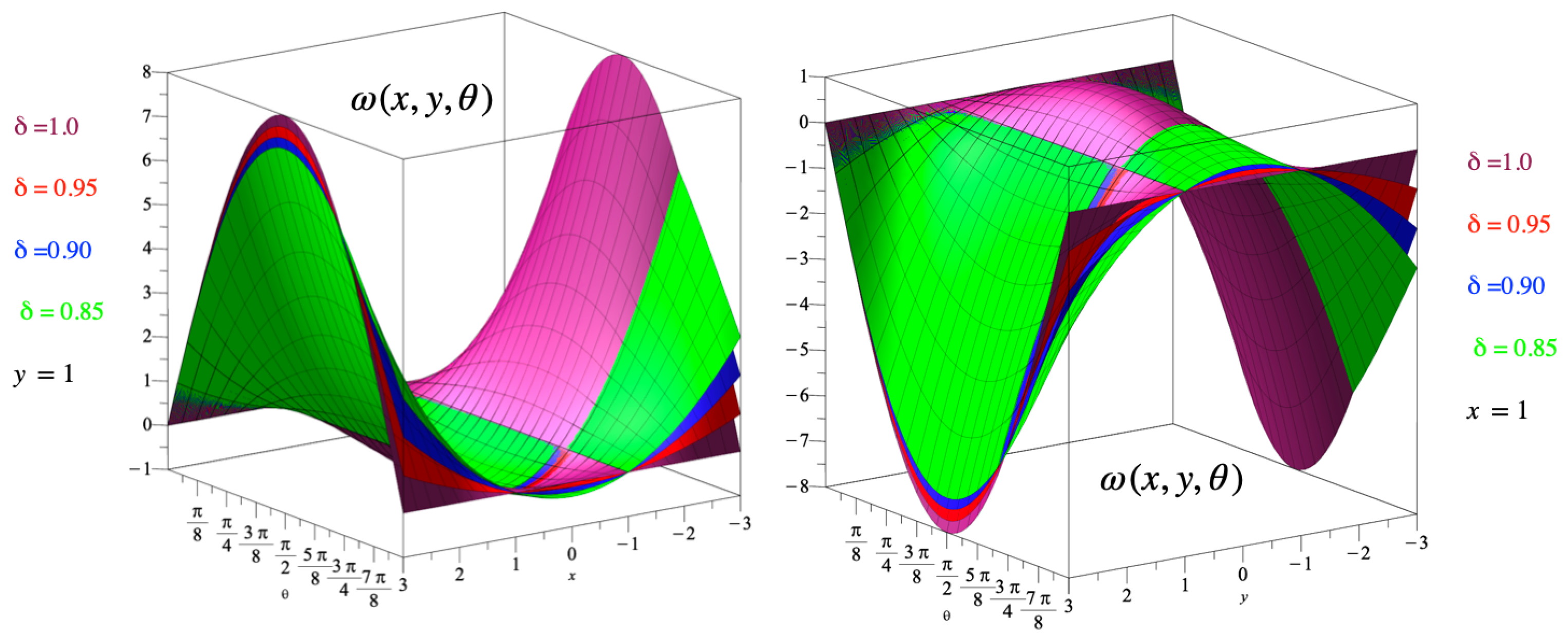
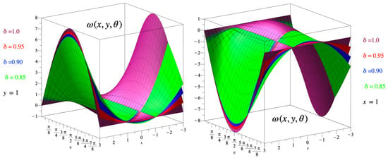
Figure 1 presents the three-dimensional plots of the approximate solution $\omega (x,y,\theta )$ for various values of $\delta .$ The exact solution of Equation (46) at $\delta =1$ is

$$\begin{array}{ccc}\hfill \omega \left(x,y,\theta \right)& =& \left(x^2-y^2\right)\left(\theta -{\displaystyle \frac{{\theta }^3}{3!}}+{\displaystyle \frac{{\theta }^5}{5!}}-{\displaystyle \frac{{\theta }^7}{7!}}+···\right)\hfill \\ \hfill \omega \left(x,y,\theta \right)& =& \left(x^2-y^2\right)sin\theta .\hfill \end{array}$$

Figure 1. The three-dimensional plots illustrate the approximate solution $\omega (x,y,\theta )$ corresponding to Example 3 for different values of $\delta$, with $\theta \in [-\pi ,\pi ]$, while the variables are fixed at $y=1$ and $x=1$, respectively.

4. The Double Natural Generalized Laplace Transform Decomposition Method for the Singular 2+1-Dimensional Non-Linear Boussinesq Equation

In this section, we present the proposed method for solving the singular 2+1-dimensional non-linear Boussinesq equation. The approach combines the double natural generalized Laplace transform (DNGLT) with the decomposition method to provide an effective solution framework.

The general form of the singular 2+1-dimensional non-linear Boussinesq equation is expressed as

$$\begin{array}{cc}\hfill {\displaystyle \frac{{\partial }^2\omega }{\partial {\theta }^2}}=& {\displaystyle \frac{1}{x}}{\left(x{\omega }_x\right)}_x+{\displaystyle \frac{1}{y}}{\left(y{\omega }_y\right)}_y+a(x,y){\omega }_{xxxx}+b(x,y){\omega }_{yyyy}\hfill \\ & +c(x,y){\omega }_{xx\theta \theta }+d(x,y){\omega }_{yy\theta \theta }+e(x,y){\omega }_{\theta }{\omega }_{xx}\hfill \\ & +g(x,y)\omega {\omega }_{xx\theta }+f(x,y,\theta ),\hfill \end{array}$$

(49)

subject to the initial conditions

$$\omega (x,y,0)=f_1(x,y),{\omega }_{\theta }(x,y,0)=f_2(x,y),$$

(50)

where $a(x,y),b(x,y),c(x,y),d(x,y),e(x,y)$, and $g(x,y)$ are arbitrary functions.

• Step 1. By first multiplying Equation (49) through by $xy$ and then applying the (DNGLT) to the modified equation together with the (DNT) of the initial conditions in Equation (50), one can, by invoking Theorem 5 and Equation (14), derive

$$\begin{array}{ccc}\hfill {\displaystyle \frac{uv}{pq{s}^2}}{\displaystyle \frac{{\partial }^2}{\partial u\partial v}}\left(uvF\left(p;u,q;v,s\right)\right)& =& {\displaystyle \frac{uv{s}^{\alpha -1}}{pq}}{\displaystyle \frac{{\partial }^2}{\partial u\partial v}}\left(uv{F}_1\left(p;u,q;v\right)\right)\hfill \\ & & +{\displaystyle \frac{uv{s}^{\alpha }}{pq}}{\displaystyle \frac{{\partial }^2}{\partial u\partial v}}\left(uv{F}_2\left(p;u,q;v\right)\right)\hfill \\ & & +{\displaystyle \frac{uv}{pq}}{\displaystyle \frac{{\partial }^2}{\partial u\partial v}}\left(uvF\left(p;u,q;v,s\right)\right)\hfill \\ & & +{\mathbf{N}}_{x,y}^{+}{G}_{\theta }\left[\Delta \right],\hfill \end{array}$$

(51)

where

$$\begin{array}{ccc}\hfill \Delta & =& y{\left(x{\omega }_x\right)}_x+x{\left(y{\omega }_y\right)}_y+a(x,y)xy{\omega }_{xxxx}+b\left(x,y\right)xy{\omega }_{yyyy}\hfill \\ & & +c\left(x,y\right)xy{\omega }_{xx\theta \theta }+d\left(x,y\right)xy{\omega }_{yy\theta \theta }+e\left(x,y\right){\omega }_{\theta }{\omega }_{xx}+g\left(x,y\right)\omega {\omega }_{xx\theta }.\hfill \end{array}$$

Streamlining Equation (51), we obtain

$$\begin{array}{ccc}\hfill {\displaystyle \frac{{\partial }^2}{\partial u\partial v}}\left(uvF\left(p;u,q;v,s\right)\right)& =& s^{\alpha +1}{\displaystyle \frac{{\partial }^2}{\partial u\partial v}}\left(uv{F}_1\left(p;u,q;v\right)\right)\hfill \\ & & +s^{\alpha +2}{\displaystyle \frac{{\partial }^2}{\partial u\partial v}}\left(uv{F}_2\left(p;u,q;v\right)\right)\hfill \\ & & +s^2{\displaystyle \frac{{\partial }^2}{\partial u\partial v}}\left(uvF\left(p;u,q;v,s\right)\right)\hfill \\ & & +{\displaystyle \frac{pq{s}^2}{uv}}{\mathbf{N}}_{x,y}^{+}{G}_{\theta }\left[\Delta \right].\hfill \end{array}$$

(52)

• Step 2. Applying the integration to both sides of Equation (52) from 0 to u and 0 to v with respect to $u,v$, then dividing the result by $uv,$ we obtain

  $$\begin{array}{ccc}\hfill F\left(p;u,q;v,s\right)& =& {\displaystyle \frac{1}{uv}}{\int }_0^u{\int }_0^v{s}^{\alpha +1}{\displaystyle \frac{{\partial }^2}{\partial u\partial v}}\left(uv{F}_1\left(p;u,q;v\right)\right)dudv\hfill \\ & & +{\displaystyle \frac{1}{uv}}{\int }_0^u{\int }_0^v{s}^{\alpha +2}{\displaystyle \frac{{\partial }^2}{\partial u\partial v}}\left(uv{F}_2\left(p;u,q;v\right)\right)dudv\hfill \\ & & +{\displaystyle \frac{1}{uv}}{\int }_0^u{\int }_0^v{s}^2{\displaystyle \frac{{\partial }^2}{\partial u\partial v}}\left(uvF\left(p;u,q;v,s\right)\right)dudv\hfill \\ & & +{\displaystyle \frac{1}{uv}}{\int }_0^u{\int }_0^v{\displaystyle \frac{pq{s}^2}{uv}}{\mathbf{N}}_{x,y}^{+}{G}_{\theta }\left[\Delta \right]dudv.\hfill \end{array}$$

  (53)
• Step 3. By employing the (IDNGLT) to Equation (53), we derive

  $$\begin{array}{ccc}\hfill \omega \left(x,y,\theta \right)& =& {\mathbf{N}}_2^{-1}{G}_s^{-1}\left[{\displaystyle \frac{1}{uv}}{\int }_0^u{\int }_0^v{s}^{\alpha +1}{\displaystyle \frac{{\partial }^2}{\partial u\partial v}}\left(uv{F}_1\left(p;u,q;v\right)\right)dudv\right]\hfill \\ & & +{\mathbf{N}}_2^{-1}{G}_s^{-1}\left[{\displaystyle \frac{1}{uv}}{\int }_0^u{\int }_0^v{s}^{\alpha +2}{\displaystyle \frac{{\partial }^2}{\partial u\partial v}}\left(uv{F}_2\left(p;u,q;v\right)\right)dudv\right]\hfill \\ & & +{\mathbf{N}}_2^{-1}{G}_s^{-1}\left[{\displaystyle \frac{1}{uv}}{\int }_0^u{\int }_0^v{s}^2{\displaystyle \frac{{\partial }^2}{\partial u\partial v}}\left(uvF\left(p;u,q;v,s\right)\right)dudv\right]\hfill \\ & & +{\mathbf{N}}_2^{-1}{G}_s^{-1}\left[{\displaystyle \frac{1}{uv}}{\int }_0^u{\int }_0^v{\displaystyle \frac{pq{s}^2}{uv}}{\mathbf{N}}_{x,y}^{+}{G}_{\theta }\left[\Delta \right]dudv\right].\hfill \end{array}$$

  (54)
• Step 4. By implementing (DNGLTDM), one can obtain

$$\begin{array}{ccc}\hfill \sum _{n=0}^{\infty }{\omega }_n\left(x,y,\theta \right)& =& {\mathbf{N}}_2^{-1}{G}_s^{-1}\left[{\displaystyle \frac{1}{uv}}{\int }_0^u{\int }_0^v{s}^{\alpha +1}{\displaystyle \frac{{\partial }^2}{\partial u\partial v}}\left(uv{F}_1\left(p;u,q;v\right)\right)dudv\right]\hfill \\ & & +{\mathbf{N}}_2^{-1}{G}_s^{-1}\left[{\displaystyle \frac{1}{uv}}{\int }_0^u{\int }_0^v{s}^{\alpha +2}{\displaystyle \frac{{\partial }^2}{\partial u\partial v}}\left(uv{F}_2\left(p;u,q;v\right)\right)dudv\right]\hfill \\ & & +{\mathbf{N}}_2^{-1}{G}_s^{-1}\left[{\displaystyle \frac{1}{uv}}{\int }_0^u{\int }_0^v{s}^2{\displaystyle \frac{{\partial }^2}{\partial u\partial v}}\left(uvF\left(p;u,q;v,s\right)\right)dudv\right]\hfill \\ & & +{\mathbf{N}}_2^{-1}{G}_s^{-1}\left[{\displaystyle \frac{1}{uv}}{\int }_0^u{\int }_0^v{\displaystyle \frac{pq{s}^2}{uv}}{\mathbf{N}}_{x,y}^{+}{G}_{\theta }\left[\sum _{n=0}^{\infty }{\Delta }_n\right]dudv\right],\hfill \end{array}$$

(55)

where ${\omega }_0\left(x,y,\theta \right)$ and ${\omega }_{n+1}\left(x,y,\theta \right)$ are imparted by

$$\begin{array}{ccc}\hfill {\omega }_0(x,y,\theta )& =& {\mathbf{N}}_2^{-1}{G}_s^{-1}\left[{\displaystyle \frac{1}{uv}}{\int }_0^u{\int }_0^v{s}^{\alpha +1}{\displaystyle \frac{{\partial }^2}{\partial u\partial v}}\left(uv{F}_1\left(p;u,q;v\right)\right)dudv\right]\hfill \\ & & +{\mathbf{N}}_2^{-1}{G}_s^{-1}\left[{\displaystyle \frac{1}{uv}}{\int }_0^u{\int }_0^v{s}^{\alpha +2}{\displaystyle \frac{{\partial }^2}{\partial u\partial v}}\left(uv{F}_2\left(p;u,q;v\right)\right)dudv\right]\hfill \\ & & +{\mathbf{N}}_2^{-1}{G}_s^{-1}\left[{\displaystyle \frac{1}{uv}}{\int }_0^u{\int }_0^v{s}^2{\displaystyle \frac{{\partial }^2}{\partial u\partial v}}\left(uvF\left(p;u,q;v,s\right)\right)dudv\right]\hfill \end{array}$$

(56)

and

$${\omega }_{n+1}(x,y,\theta )={\mathbf{N}}_2^{-1}{G}_s^{-1}\left[{\displaystyle \frac{1}{uv}}{\int }_0^u{\int }_0^v{\displaystyle \frac{pq{s}^2}{uv}}{\mathbf{N}}_{x,y}^{+}{G}_{\theta }\left[\sum _{n=0}^{\infty }{\Delta }_n\right]dudv\right].$$

(57)

Now, we assume that the inverse (DNGLT) with respect to $p,q,u,v$, and s exists for Equations (56) and (57).

To confirm the applicability of the proposed method for 2+1-dimensional coupled-system Boussinesq equations, we present the following example with $a=b=c=d=e=-1$:

Example 4.

The 2+1-dimensional coupled-system Boussinesq equation is imparted by

$$\begin{array}{ccc}\hfill {\displaystyle \frac{{\partial }^2\omega }{\partial {\theta }^2}}& =& {\displaystyle \frac{1}{x}}{\left(x{\omega }_x\right)}_x+{\displaystyle \frac{1}{y}}{\left(y{\omega }_y\right)}_y{\omega }_{xxxx}-{\omega }_{yyyy}\hfill \\ & & +{\omega }_{xx\theta \theta }+{\omega }_{yy\theta \theta }+{\omega }_{\theta }{\omega }_{xx}-\omega {\omega }_{xx\theta }\hfill \\ & & +\left(x^2-y^2\right)e^{\theta },\hfill \end{array}$$

(58)

with initial conditions

$$\omega \left(x,y,0\right)=\left(x^2-y^2\right),{\omega }_{\theta }\left(x,y,0\right)=\left(x^2-y^2\right).$$

(59)

In order to obtain the solution to the Equation (58), applying our method, one can get

$$\begin{array}{ccc}\hfill {\omega }_0(x,y,\theta )& =& {\mathbf{N}}_2^{-1}{G}_s^{-1}\left[{\displaystyle \frac{1}{uv}}{\int }_0^u{\int }_0^v{s}^{\alpha +1}\left({\displaystyle \frac{6u^2}{p^{3}q}}-{\displaystyle \frac{6v^2}{p{q}^3}}\right)dudv\right]\hfill \\ & & +{\mathbf{N}}_2^{-1}{G}_s^{-1}\left[{\displaystyle \frac{1}{uv}}{\int }_0^u{\int }_0^v{s}^{\alpha +2}\left({\displaystyle \frac{6u^2}{p^{3}q}}-{\displaystyle \frac{6v^2}{p{q}^3}}\right)dudv\right]\hfill \\ & & +{\mathbf{N}}_2^{-1}{G}_s^{-1}\left[\begin{array}{c}{\displaystyle \frac{1}{uv}}{\int }_0^u{\int }_0^v{s}^2\left({\displaystyle \frac{6u^2}{p^{3}q}}-{\displaystyle \frac{6v^2}{p{q}^3}}\right)\\ \left(s^{\alpha +1}+s^{\alpha +2}+s^{\alpha +3}+\cdots \right)dudv\end{array}\right],\hfill \end{array}$$

(60)

where

$$\begin{array}{ccc}\hfill G_{\theta }\left(e^{\theta }\right)& =& G_{\theta }\left(1+\theta +{\displaystyle \frac{{\theta }^2}{2!}}+{\displaystyle \frac{{\theta }^3}{3!}}\cdots \right)\hfill \\ & =& s^{\alpha +1}+s^{\alpha +2}+s^{\alpha +3}+\cdots ,\hfill \end{array}$$

Hence

$$\begin{array}{ccc}\hfill {\omega }_0(x,y,\theta )& =& \left(x^2-y^2\right)+\left(x^2-y^2\right)\theta \hfill \\ & & +\left(x^2-y^2\right)\left({\displaystyle \frac{{\theta }^2}{2!}}+{\displaystyle \frac{{\theta }^3}{3!}}+{\displaystyle \frac{{\theta }^4}{4!}}\cdots \right),\hfill \end{array}$$

(61)

and

$${\omega }_{n+1}(x,y,\theta )={\mathbf{N}}_2^{-1}{G}_s^{-1}\left[{\displaystyle \frac{1}{uv}}{\int }_0^u{\int }_0^v{\displaystyle \frac{pq{s}^2}{uv}}{\mathbf{N}}_{x,y}^{+}{G}_{\theta }\left[\sum _{n=0}^{\infty }{\Delta }_n\right]dudv\right]$$

(62)

where ${\Delta }_n$ dominated by

$$\begin{array}{ccc}\hfill {\Delta }_n& =& y{\left(x{\omega }_{nx}\right)}_x+x{\left(y{\omega }_{ny}\right)}_y-xy{\omega }_{nxxxx}-xy{\omega }_{nyyyy}\hfill \\ & & +xy{\omega }_{nxx\theta \theta }+xy{\omega }_{nyy\theta \theta }+{\omega }_{n\theta }{\omega }_{nxx}-{\omega }_n{\omega }_{nxx\theta }.\hfill \end{array}$$

In particular, at $n=0,$ Equation (62), becomes

$${\omega }_1(x,y,\theta )={\mathbf{N}}_2^{-1}{G}_s^{-1}\left[{\displaystyle \frac{1}{uv}}{\int }_0^u{\int }_0^v{\displaystyle \frac{pq{s}^2}{uv}}{\mathbf{N}}_{x,y}^{+}{G}_{\theta }\left[{\Delta }_0\right]dudv\right],$$

(63)

where ${\Delta }_0$ is given by

$$\begin{array}{ccc}\hfill {\Delta }_0& =& y{\left(x{\omega }_{0x}\right)}_x+x{\left(y{\omega }_{0y}\right)}_y-xy{\omega }_{0xxxx}-xy{\omega }_{0yyyy}\hfill \\ & & +xy{\omega }_{0xx\theta \theta }+xy{\omega }_{0yy\theta \theta }+{\omega }_{0\theta }{\omega }_{0xx}-{\omega }_0{\omega }_{0xx\theta }.\hfill \end{array}$$

Therefore

$$\begin{array}{ccc}\hfill {\omega }_1& =& {\mathbf{N}}_2^{-1}{G}_s^{-1}\left[{\displaystyle \frac{1}{uv}}{\int }_0^u{\int }_0^v{\displaystyle \frac{pq{s}^2}{uv}}{\mathbf{N}}_{x,y}^{+}{G}_{\theta }\left[{\Delta }_0\right]dudv\right],\hfill \\ \hfill {\omega }_1& =& 0.\hfill \end{array}$$

(64)

Likewise, the rest of the terms are granted by

$${\omega }_2=0,{\omega }_3=0,{\omega }_4=0,\dots$$

Hence, by utilizing Equation (42) the series solutions are achieved by

$$\begin{array}{ccc}\hfill \omega (x,y,\theta )& =& \sum _{n=0}^{\infty }{\omega }_n\left(x,y,\theta \right)={\omega }_0+{\omega }_1+{\omega }_2+\cdots \hfill \\ & =& \left(x^2-y^2\right)+\left(x^2-y^2\right)\theta ++\left(x^2-y^2\right)\left({\displaystyle \frac{{\theta }^2}{2!}}+{\displaystyle \frac{{\theta }^3}{3!}}+{\displaystyle \frac{{\theta }^4}{4!}}···\right)\hfill \\ \hfill \omega (x,y,\theta )& =& \left(x^2-y^2\right)e^{\theta }.\hfill \end{array}$$

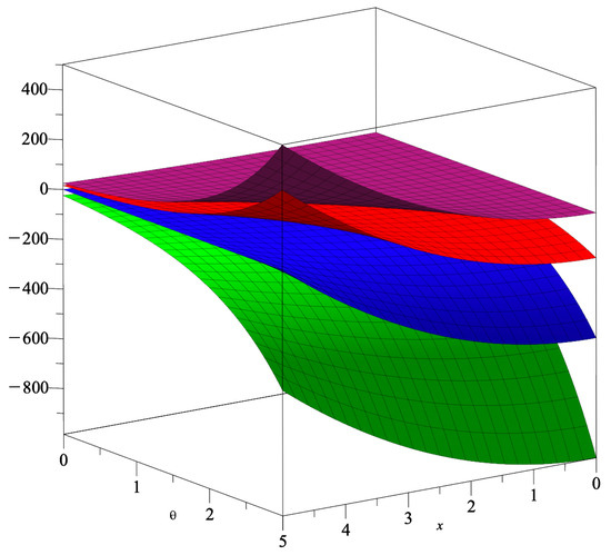
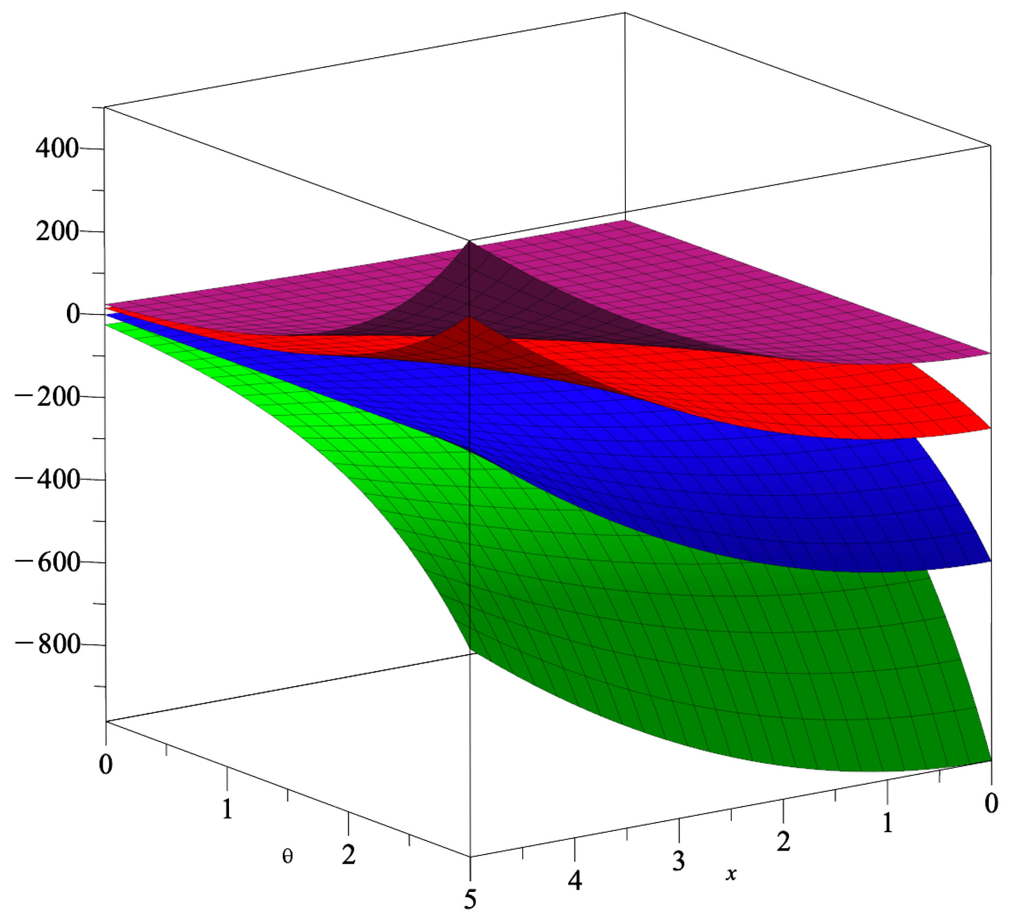
Figure 2 presents the three-dimensional plots of the approximate solution $\omega (x,y,\theta )$ over the domain $x\in [0,5]$ and $\theta \in [0,5]$, for the fixed values $y=0$ (maroon), $y=3$ (red), $y=5$ (blue), and $y=7$ (green).

Figure 2. The 3D plots of $\omega (x,y,\theta )$ in Example 4 are generated over the domain $x\in [0,5]$ and $\theta \in [0,5]$, for the fixed values $y=0$ (maroon), $y=3$ (red), $y=5$ (blue), and $y=7$ (green).

5. Conclusions

This study presents several key contributions. First, the double natural generalized Laplace transform (DNGLT) is introduced, and its fundamental properties are established, including conditions for existence, the convolution theorem, and the periodic theorem. Next, the double natural generalized Laplace transform decomposition method (DNGLTDM) is developed by combining the DNGLT with the decomposition approach. Two examples show that the proposed method works and is correct. We examined the singular fractional two-dimensional Boussinesq equation in the first example and the non-linear singular two-dimensional Boussinesq equation in the second example. We use Maple software 2021 to sketch the exact and approximate solutions. Finally, future research will focus on extending this technique to fractional problems arising in physics and related scientific fields.

References

1. Zabusky, N.J. Nonlinear Partial Differential Equations; Academic Press: New York, NY, USA, 1967. [Google Scholar]
2. Gal, C.G.; Miranville, A. Uniform global attractors for non-isothermal viscous and non-viscous Cahn-Hilliard equations with dynamic boundary conditions. Nonlinear Anal. Real World Appl. 2009, 10, 1738–1766. [Google Scholar] [CrossRef] [Scilit]
3. Kato, T.; Nishida, T. A mathematical justification for Korteweg-de Vries equation and Boussinesq equation of water surface waves. Osaka J. Math. 1986, 23, 389–413. [Google Scholar]
4. Sun, L.; Wang, Z.; Wei, Y. A second–order approximation scheme for Caputo–Hadamard derivative and its application in fractional Allen–Cahn equation. Commun. Anal. Mech. 2025, 17, 630–661. [Google Scholar] [CrossRef] [Scilit]
5. Nguyen, H.T.; Vo, V.T. Existence and uniqueness of the solution to Caputo-Hadamard differential equations with delay and nonlocal conditions. Commun. Anal. Mech. 2025, 17, 725–748. [Google Scholar] [CrossRef] [Scilit]
6. Prakasha, D.G.; Malagi, N.S.; Veeresha, P. New approach for fractional Schrodinger-Boussinesq equations with Mittag-Leffler kernel. Math. Methods Appl. Sci. 2020, 43, 9654–9670. [Google Scholar] [CrossRef] [Scilit]
7. Wazwaz, A.M. Construction of soliton solutions and periodic solutions of the Boussinesq equation by the modified decomposition method. Chaos Solitons Fractals 2001, 12, 1549–1556. [Google Scholar] [CrossRef] [Scilit]
8. Chen, F.; Liu, Q. Modified asymptotic Adomian decomposition method for solving Boussinesq equation of groundwater flow. Appl. Math. Mech. 2014, 35, 481–488. [Google Scholar] [CrossRef] [Scilit]
9. Attili, B.S. The Adomian decomposition method for solving the Boussinesq equation arising in water wave propagation. Numer. Method Partial Differ. Equ. 2006, 22, 1337–1347. [Google Scholar] [CrossRef] [Scilit]
10. Wazwaz, A.-M. New travelling wave solutions to the Boussinesq and the KleinGordon equations. Commun. Nonlinear Sci. Numer. Simul. 2008, 13, 889–901. [Google Scholar] [CrossRef] [Scilit]
11. Fernandez, F.M. On the homotopy perturbation method for Boussinesq-like equations. Appl. Math. Comput. 2014, 230, 208–210. [Google Scholar] [CrossRef] [Scilit]
12. Mukhtar, S. Numerical Analysis of the Time-Fractional Boussinesq Equation in Gradient Unconfined Aquifers with the Mittag-Leffler Derivative. Symmetry 2023, 15, 608. [Google Scholar] [CrossRef] [Scilit]
13. Algahtani, O. Theoretical and numerical analysis of nonlinear Boussinesq equation under the fractal fractional derivative. Nonlinear Eng. 2023, 12, 20220338. [Google Scholar] [CrossRef] [Scilit]
14. Gupta, A.K.; Ray, S.S. Comparison between homotopy perturbation method and optimal homotopy asymptotic method for the soliton solutions of Boussinesq–Burger equations. Comput. Fluids 2014, 103, 34–41. [Google Scholar] [CrossRef] [Scilit]
15. Lu, D.; Shen, J.; Cheng, Y. The approximate solutions of nonlinear Boussinesq equation. J. Phys. Conf. Ser. 2016, 710, 012001. [Google Scholar] [CrossRef] [Scilit]
16. Patel, H.S.; Meher, R. Application of Laplace Adomian Decomposition Method for the soliton solutions of Boussinesq-Burger equations. Int. J. Adv. Appl. Math. Mech. 2015, 3, 50–58. [Google Scholar]
17. Rady, A.S.A.; Osman, E.S.; Khalfallah, M. On soliton solutions of the (2+1) dimensional Boussinesq equation. Appl. Math. Comput. 2012, 219, 3414–3419. [Google Scholar]
18. Rawashdeh, M.; Maitama, S. Solving coupled system of nonlinear pde’s using the Natural decomposition method. Int. J. Pure Appl. Math. 2014, 92, 757–776. [Google Scholar]
19. Kiliciman, A.; Omran, M. On double Natural transform and its applications. J. Nonlinear Sci. Appl. 2017, 10, 1744–1754. [Google Scholar] [CrossRef] [Scilit]
20. Belgacem, F.B.M.; Silambarasan, R. Theory of the Natural transform. Math. Eng. Sci. Aerosp. (MESA) J. 2012, 3, 99–124. [Google Scholar]
21. Khan, Z.H.; Khan, W.A. N-transform properties and applications. NUST J. Eng. Sci. 2008, 1, 127–133. [Google Scholar]
22. Kim, H. The intrinsic structure and properties of Laplace-typed integral transforms. Math. Probl. Eng. 2017, 2017, 1762729. [Google Scholar] [CrossRef] [Scilit]
23. Gadain, H.E. Application of Double Natural Decomposition Method for Solving Singular One-Dimensional Boussinesq Equation. Filomat 2018, 32, 4389–4401. [Google Scholar] [CrossRef] [Scilit]
24. Khan, H.; Shah, R.; Kumam, P.; Baleanu, D.; Arif, M. Laplace decomposition for solving nonlinear system of fractional order partial differential equations. Adv. Differ. Equ. 2020, 2020, 375. [Google Scholar] [CrossRef] [Scilit]
25. Bayrak, M.; Demir, A. A new approach for space-time fractional partial differential equations by residual power series method. Appl. Math. Comput. 2018, 336, 215–230. [Google Scholar] [CrossRef] [Scilit]
26. Eltayeb, H. Application of Natural Generalized-Laplace Transform and Its Properties. Mathematics 2025, 13, 3194. [Google Scholar] [CrossRef] [Scilit]
Disclaimer/Publisher’s Note: The statements, opinions and data contained in all publications are solely those of the individual author(s) and contributor(s) and not of MDPI and/or the editor(s). MDPI and/or the editor(s) disclaim responsibility for any injury to people or property resulting from any ideas, methods, instructions or products referred to in the content.
Article Metrics
Citations
Article Access Statistics
Multiple requests from the same IP address are counted as one view.