


Abstract
Controllers for processes with fractional-order delay are usually tuned and evaluated with Padé and Oustaloup approximations. For integrating processes with the delay exp(−√s), this paper makes two contributions. It proposes a fractional lead-filtered FOPD (FLF-FOPD) controller, whose two lead elements provide a phase lead that grows like the process lag, and evaluates it and competing controllers on the exact process, revealing two pitfalls of the usual simulation chain. The Padé approximant fails above a closed-form frequency limit; the loop gain beyond it is small for 27 of 28 examined designs, but for the original FLF-FOPD tuning the phase margin was computed as 13.6° instead of 66.7°. The refined Oustaloup filter in FOMCON has a mid-band gain error (d/b)r that shortens the simulated delay by about 10% and made eight reproducible ITAE values from one study 8–22% too optimistic. In a benchmark with Ms ≤ 1.4, a bounded noise-to-control gain Mu and a 20 s horizon, the FLF-FOPD reduces to an FOPD for Mu ≤ 50. At Mu ≈ 860, the best of 60 runs lowers ITAE by a factor of 2.5 relative to the FOPD limit, at the cost of 3.5 times more control-signal noise, instability for α ≥ 0.7 and no benefit under saturation.
1. Introduction
Integrating processes with long or distributed delays are among the most difficult single-loop control problems in the process industry. The pole at the origin removes the natural damping of the process, while the delay limits the achievable bandwidth. When the delay arises from diffusion or transport through a distributed medium, as in heat conduction, mass diffusion or lossy transmission lines, the transfer function contains irrational terms of the form exp (−(τs)α) with 0 < α < 1, usually called a fractional-order time delay (FOTD) [1,2]. For α = 0.5, this factor is the exact transfer function of a semi-infinite diffusion medium. Its behaviour differs markedly from that of a pure dead time: the gain decays as exp (−√(ω/2)) instead of remaining at unity, and the phase lag grows only as √ω.
Fractional-order (FO) controllers have frequently been proposed for such processes, since non-integer integral and derivative orders provide additional freedom for loop shaping [3,4,5,6]. FOPI, FOPID, predictive FOPI (FOPPI) and filtered FOPI controllers have recently been tuned for FOTD processes by metaheuristic minimisation of the integral of time-weighted absolute error (ITAE) [7,8,9,10,11]. Fractional lead elements, a classical means of counteracting delay-induced phase lag [12], have also been combined in series with FO PI or PD controllers for integrating dead-time processes [13] and other time-delayed processes [14]. Earlier work treated stabilisation and PI/PID design for fractional-order plants with time delay [15] and frequency-domain FOPI design for integrating dead-time processes [16], and recent contributions combine bibliometric surveys with simulation studies of FOPID control [17]. In most of these studies, the FO operators of the controller and the FOTD term of the plant are implemented in MATLAB/Simulink with low-order Padé approximants of the exponential and Oustaloup-type rational approximations of sα [18,19,20], and ITAE values are compared across controllers whose parameters were obtained from different sources and tuning procedures. The accuracy of the operator approximations themselves has been compared in detail [21,22], and numerical inverse Laplace transformation has been proposed for the time response of irrational closed loops [23], but the consequences of the approximations for the reported controller performance, and for comparisons between controllers, have received little attention. Table 1 summarises the studies closest to the present one.
Table 1.
Studies closest to the present work. FOTD: delay exp(−(τs)α) with α < 1; FO plant: fractional-order plant dynamics with integer-order dead time.
This paper has two aims of equal weight. The first is methodological: to determine how far the standard Padé–Oustaloup simulation chain can be trusted for this process class and to provide a procedure that avoids its pitfalls. The second is to propose and assess a fractional-order lead filter in series with an FOPD controller (FLF-FOPD) for the integrating distributed-parameter system (DPS) with α = 0.5. The structure was first developed in the MSc thesis of the second author [25]. The two aims are connected: the FLF-FOPD is the case that exposed the pitfalls, and its value can only be judged once they are removed. The design idea is straightforward. Because the phase lag of exp(−√s) keeps increasing with frequency, the controller should provide a phase lead that also increases across the crossover region, and two fractional lead elements with different orders and corner frequencies can achieve this over a wider band than a single fractional derivative. No integral term is included, since the process itself is integrating.
A reliable evaluation of the controller proved to be more demanding than its design. An initial evaluation following the usual procedure gave an ITAE about four times lower than that of the best competitor. This advantage is confirmed on the exact plant, but it was obtained with a noise-to-control gain of 4611, the competing settings had been tuned under different conditions, and the stability margins and transient responses reported with it were artefacts of the approximate plant model. Closer analysis revealed four issues, all of which concern other controllers and other studies of this process class as well:
- The second-order Padé approximant of exp(−√s) reproduces the phase at low frequencies, but its magnitude returns to unity at high frequencies, whereas the true magnitude is below 10−3 above 100 rad/s. For controllers with appreciable high-frequency gain, such as any FO derivative action, the approximate loop therefore acquires spurious gain crossovers. In our case, this led to a phase margin of 13.6° instead of 66.7° and to a predicted instability for a 50% increase in process gain, although the actual loop is well damped.
- The refined Oustaloup filter of Xue et al. [18], as implemented in the new_fod function of the FOMCON toolbox [19] and used to realise (τs)α inside the Padé block, has a mid-band gain of (d/b)α instead of one. With the usual values b = 10 and d = 9, this is equivalent, to first order, to simulating the delay parameter as 0.9τ. Time-domain results obtained in this way therefore describe a process with a shorter delay and are usually optimistic.
- Minimising ITAE without any constraint on robustness or on the amplification of measurement noise into the control signal favours unbounded high-frequency gain. The optimiser then exploits the upper corner frequency of the Oustaloup band, so that the reported performance reflects a numerical setting rather than the controller structure.
- Benchmark parameters are often taken from earlier papers that used other objectives, bounds or optimisers, while the proposed controller is tuned anew, and metaheuristics are frequently run only once with a fixed seed.
The first two issues relate to the simulation model rather than to the controllers. To assess their effect on reported results, we re-evaluated 28 designs from four sources, three external and one from our own earlier work, on the exact plant (Section 3.1). The Padé approximant proved adequate for 27 of them, because their approximate loop gain is small in the frequency range where the approximant fails; a closed-form validity limit that predicts this is derived in Section 2.2.2. The Oustaloup gain error, in contrast, biased all eight reported ITAE values that we were able to reproduce exactly [7] by 8–22%. The ranking of the controllers was not affected in the cases examined, but the absolute values were.
The contributions on the evaluation side are as follows:
- A closed-form estimate of the validity limit of Padé approximants of the FOTD term, ω*τ = zn(1/α), where zn depends only on the Padé order and the admissible error, combined with a loop-gain check for spurious crossovers and applied to 28 designs from four sources;
- The identification of a mid-band gain error (d/b)r in the refined Oustaloup filter as implemented in FOMCON, which shifts the simulated delay parameter by about 10% and biased the reproducible ITAE values of [7] by 8–22%;
- A wide-band rational model of the FOTD term with 60 real poles and exact static gain, validated against high-precision numerical inverse Laplace transformation of the exact loop, which can replace the Padé–Oustaloup block in Simulink models.
The contributions on the controller side are as follows:
- The FLF-FOPD controller for integrating processes with fractional-order delay, together with a phase-lead design rationale; the structure is related to known series lead and PI–PD structures [12,13,14], and its novelty lies in its application to this process class and in the conditions under which it is useful;
- A statistically supported comparison of the FLF-FOPD with PI, FOPD, FOPID and predictive PI controllers, all retuned under identical conditions with a common roll-off filter and constraints on Ms and Mu. Under a moderate noise-gain limit, the FLF-FOPD reduces to an FOPD and offers no benefit, and a retuned FOPPI gives the best servo design; at noise gains above about 150, its best design lowers ITAE by up to a factor of 2.5, and the costs of this improvement are quantified.
The paper is organised as follows. Section 2 describes the process, its numerical realisation (including the Padé validity limit and the Oustaloup gain error), the proposed controller with the competing structures, and the evaluation procedure. The results are presented in Section 3 and discussed in Section 4, and Section 5 concludes the paper.
2. Materials and Methods
2.1. Process Model
The considered process is the integrating DPS with fractional-order delay studied in [7,9]:
The irrational factor has a clear physical interpretation. For one-dimensional diffusion ∂T/∂t = κ ∂2T/∂x2 in a semi-infinite medium driven at x = 0, the transfer function from the boundary to a point at depth ℓ is exp (−ℓ√(s/κ)), i.e., the factor above with α = 0.5 and τ = ℓ2/κ [1,2]. The integrator represents a quantity that accumulates downstream, such as a liquid level or stored energy.
For α = 0.5, the step response of the delay factor is erfc (1/(2√(t/τ))), which has no dead time but rises slowly and has a long tail. The frequency response is
so that the magnitude decays faster than any power of ω, while the phase lag grows only as √ω (−41° at 1 rad/s, −128° at 10 rad/s and −405° at 100 rad/s). A pure dead time behaves in the opposite way, with unit magnitude and a linearly growing phase lag. This difference is important for Section 2.2: a controller with large high-frequency gain can be stable with the true plant, whose magnitude vanishes at high frequencies, and yet unstable with an approximant whose magnitude does not.
All frequency-domain quantities in this paper, i.e., gain, phase and delay margins and peak sensitivities, are computed from this exact expression, and all time-domain results are checked against the fixed Talbot inversion [26] of the exact closed loop.
The values Kg = 1 and τ = 1 s involve no loss of generality. With the normalised variables = τs and = t/τ, the process becomes Kgτ exp (−)/, so that α is the only parameter that changes the problem. A controller designed for Kg = 1 and τ = 1 s gives the same loop transfer function, and therefore the same Ms, phase and gain margins and the same normalised responses, for any Kg and τ if its parameters are mapped as K2 → K2τα1, K3 → K3τα2/(Kgτ) and K4 → K4/(Kgτ); for the other structures, Kp → Kp/(Kgτ), Kd → Kdτμ/(Kgτ) and Ki → Kiτ(−λ)/(Kgτ). Crossover frequencies then scale with 1/τ, the ITAE scales with τ2 and the noise-to-control gain Mu scales with 1/(Kgτ), and the Padé validity limit of Section 2.2.2 is already given in the dimensionless form ω*τ. The mapping is exact for ideal fractional operators. The claim of no loss of generality refers to the loop transfer function and to all quantities derived from it; it holds for the constrained tuning problem of Section 2.4 only if every element that carries a physical frequency or amplitude is transformed as well. Specifically, the Oustaloup band [ωb, ωh] and the corner frequency of the common roll-off filter must scale with 1/τ, the sampling period of a digital implementation with τ, the constraint Mu ≤ Mumax must be replaced by Mu ≤ Mumax/(Kgτ) because Mu has the units of the inverse process gain, and actuator limits and noise levels must be expressed relative to Kg. Ms is dimensionless and needs no rescaling. With these transformations the admissible sets of the normalised and the physical problem correspond one to one, so that their constrained optima coincide. If, instead, a fixed realisation band, filter or Mu limit is kept while τ or Kg changes, the loop shapes still map onto each other, but the admissible controller families and hence the constrained optima are different, and the results of this paper do not transfer directly.
2.2. Numerical Realisation of the Fractional-Order Delay
The commonly used second-order Padé realisation of exp(−√s) is accurate up to about 5 rad/s, but its magnitude is wrong by several orders of magnitude at higher frequencies. The wide-band model proposed below matches the exact response from 10−4 rad/s up to the frequency at which the delay magnitude falls below 10−6, about 380 rad/s (Figure 1).
Figure 1.
Frequency response of the fractional-order delay factor exp(−√s): exact, second-order Padé + refined Oustaloup realisation, and the proposed 60-pole wide-band model. (a) Magnitude; (b) phase. The wide-band model is plotted where |D| > 10−6 (ω ≲ 380 rad/s); below that level its absolute error, about 2 × 10⁻⁷, dominates (Table 2). The shaded region marks the validity range of the second-order Padé approximant, ω* < 4.2 rad/s (5% error, Table 3).
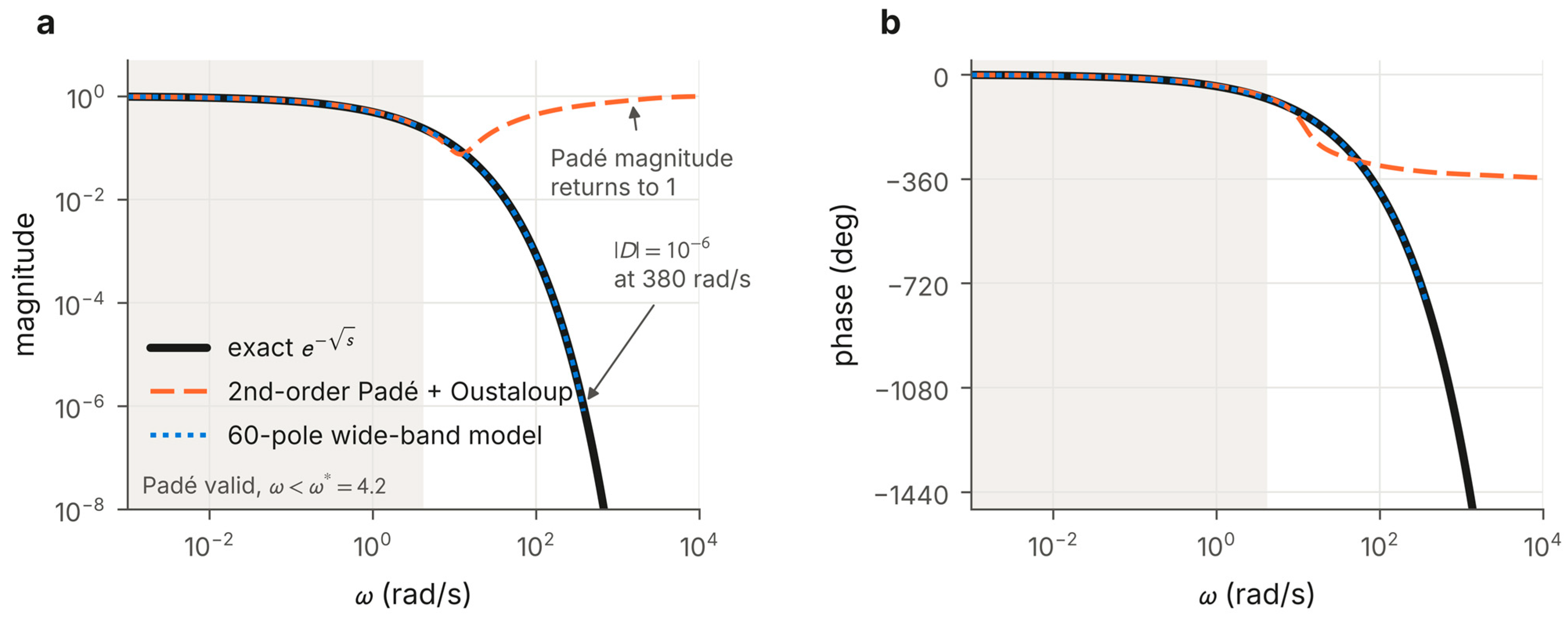
Table 2.
Magnitude of the delay factor exp(−√s) and of its realisations.
Table 3.
Validity limit of the [n/n] Padé approximant of exp (−(τs)α) for a 5% relative error: closed-form zn and ω*τ obtained from the numerically computed crossing of ε = 0.05.
2.2.1. Padé–Oustaloup Realisation
Following [7,19], the exponential is first replaced by its second-order Padé approximant in the variable x = (τs)α,
and the remaining sα terms are realised with the refined Oustaloup filter of Xue et al. [18] (N = 5, band 10−3–103 rad/s, b = 10, d = 9), as implemented in the FOMCON toolbox for MATLAB, version 1.21b [19]. In [25], and in our reproduction of [7], this block is followed by a first-order filter 1/(10−3s + 1).
The Padé approximant is a rational function of x whose magnitude tends to one as |x| increases. On the imaginary axis, x = √(jωτ) is not purely imaginary, so the approximant is not exactly all-pass, but its magnitude still approaches unity, whereas the true magnitude tends to zero. Table 2 quantifies the difference.
Evaluated with the exact x, the Padé approximant is adequate up to about 5 rad/s, where its magnitude error is about 4% and its phase error is about 4°. At higher frequencies, the phase error increases rapidly (10.5° at 7 rad/s and 27° at 10 rad/s). At 100 rad/s, the realisation overestimates the plant gain by a factor of about 500, and at 1000 rad/s, the upper edge of the Oustaloup band used for the controllers, by more than nine orders of magnitude. A controller whose gain at these frequencies is comparable to its low-frequency gain is therefore assessed on a plant that does not exist.
2.2.2. A General Validity Limit for Padé Approximants of the FOTD Term
The limit of about 5 rad/s found above can be generalised. Let Pn (x) denote the [n/n] Padé approximant of e(−x) and define its relative error as ε(x) = |Pn (x)ex − 1|. This complex measure combines magnitude and phase errors; ε = 0.05 corresponds to about 5% in magnitude or 2.9° in phase. For small |x|, the classical error expansion of the Padé approximant, Pn (x)ex − 1 = (−1)n cn x(2n+1) + O(x(2n+3)), gives the asymptotic estimate
in which the sign (−1)n of the leading coefficient drops out because ε is a modulus. The error therefore exceeds a tolerance ε at |x| ≈ zn, the (2n + 1)-th root of ε/cn. Since |x| = (ωτ)α on the imaginary axis, the estimated validity limit is
Equation (5) follows from Equation (4) by solving cn zn(2n+1) = ε and using |x| = (ωτ)α. For the second-order approximant, c2 = 1/720, so that z2 = (720ε)(1/5) = 2.05 for ε = 0.05 (Table 3). Equation (5) is an asymptotic estimate, not a rigorous bound: it neglects the higher-order terms and the dependence of ε on the argument of x. Its accuracy is therefore assessed numerically below, and it should be used to locate the limit rather than to certify it.
The argument of x, απ/2, has only a small influence. For 0.3 ≤ α ≤ 0.9, the numerically computed crossing of ε = 0.05 differs from zn by less than 8% for n ≤ 3 and by less than 11% for n ≤ 5 (Table 3); because ω* depends on zn(1/α), the corresponding error in ω* can reach 14% for small α. Through the exponent 1/α, the limit depends strongly on the delay order. For α = 0.5 and τ = 1 s, it is 4.2 rad/s for n = 2 and 11 rad/s for n = 3, whereas for α = 0.3 a second-order approximant remains adequate up to 10 rad/s.
Whether an analysis is reliable depends not only on this limit but also on the loop gain beyond it. We therefore use the following check: the largest magnitude of the approximate loop, |(jω)| = |C(jω)G0(jω)Pn(x(jω))|, is computed for ω* < ω ≤ 103 rad/s, where G0 is the rational part of the process and 103 rad/s is the upper edge of the controller realisation. If this value is well below one, the approximate loop has no spurious gain crossovers and its phase margin can be trusted, although the gain margin may still differ by a few decibels, since it depends on the loop gain near the phase crossover. If the value approaches or exceeds one, spurious crossovers appear, and a higher Padé order helps only if ω* is moved beyond the band in which the loop gain is significant (Section 3.2).
2.2.3. Gain Error of the Refined Oustaloup Filter
The refined Oustaloup filter [18], as implemented in new_fod of FOMCON [19] and used by its refined approximation option, approximates sr over [ωb, ωh] by
with the usual Oustaloup corner frequencies ωk′ and ωk. Within the band, the second factor is close to one because the term b ωh|s| dominates, and the product behaves as (s/ωh)r. Consequently, ŝr ≈ (dωh/b)r (s/ωh)r = (d/b)r sr. With the default values b = 10 and d = 9, the realised operator is therefore too small by the constant factor 0.9r, i.e., by 2.6% for r = 0.25, 5.1% for r = 0.5 and 9.0% for r = 0.9 (Figure 2a). The filters in the Simulink models of [25] have this gain, and the published results of [7] can be reproduced only with it (Section 3.1).
Figure 2.
(a) Mid-band gain error of the refined Oustaloup filter (N = 5, band 10−3–103 rad/s shaded, b = 10, d = 9): realised magnitude divided by ωr for four orders; dotted lines show (d/b)r. (b) ITAE of the eight designs of [7] as reported (Padé–Oustaloup chain) and on the exact plant, for the integrating and the first-order process. Panel (b) uses each design’s own controller realisation.
In a controller, this error is of little consequence, because it is absorbed into the tuned gain as long as the same realisation is used for tuning and implementation. In the plant model, the situation is different. Realising x = (τs)α with ŝα replaces x by (d/b)α τα sα = ((d/b)τ s)α in the linear term of the Padé approximant. Higher powers of x are realised as integer powers of s multiplied by a fractional operator and do not carry the full factor; for α = 0.5, for instance, x2 = τs is realised exactly. To first order in x, and hence at the low frequencies that determine the step response, the simulated process therefore has the delay parameter (d/b)τ = 0.9τ, irrespective of α. As the Padé approximant is accurate in this frequency range, a study based on this realisation effectively simulates a process with about 10% less delay than the one it describes. Section 3.1 shows that this accounts for most of the bias in the reported ITAE values, the remainder (at most 4%) being due to the Padé approximant. The error is removed by multiplying the filter by (b/d)r. The constant factor follows from the formula of [18] itself, i.e., Equation (6), which new_fod implements directly; the FOMCON and FOTF versions of new_fod realise the same formula [21]. It is therefore not specific to a version of the toolbox: any realisation of Equation (6) with b = 10 and d = 9 has the same mid-band gain. A numerical check is simple: the call new_fod(0.5, 5, 1e-3, 1e3, 10, 9) returns a filter whose magnitude at ω = 1 rad/s is 0.9487 = 0.90.5 instead of 1, with a phase of 45.04°. Wiora and Wiora [21] compared the classical, the refined and a later variant of the Oustaloup filter [27] and reported magnitude errors of the refined filter of up to about 10%, but did not trace them to a constant factor; the classical filter and the later variant were not examined here. In this paper, the correction is applied to the plant realisation only. In the controllers, it is not needed, because all controller gains are tuned and reported for the realised operators, so that the factor is absorbed in the gains (Section 2.3). In a Simulink model, the correction is a gain block (10/9)r in series with each refined Oustaloup block of order r in the plant model.
2.2.4. Wide-Band Rational Model
The delay factor is approximated by a sum of first-order terms with fixed, logarithmically spaced real poles pk. The residues rk are obtained by weighted linear least squares on a dense frequency grid, subject to the equality constraint Σ rk = 1, which makes the static gain exactly one:
The fit uses 4000 frequencies between 10−4 and 105 rad/s with the weight 1/max(|D(jω)|, 10−4), so that the relative error is controlled wherever the response is significant. This is a simplified form of vector fitting [28] with fixed poles, which leads to a linear equality-constrained least-squares problem with a unique solution. Without the constraint the residues sum to 0.86, i.e., the static gain is in error by 14% even though the fit error above 10−4 rad/s is small; for integrating loops, whose steady state depends on the static gain of the delay, this matters. The model is stable by construction and is implemented as a diagonal state-space block. Wherever |D(jω)| > 10−3, it reproduces the exact response with a maximum absolute error of 2.9 × 10⁻⁴, a relative error below 0.12% and a phase error below 0.06°. Its unit-step response agrees with erfc (1/(2√t)) within 4.1 × 10⁻⁵ for 0.05 ≤ t ≤ 20 s, and the fixed-Talbot inversion reproduces the same response within 2 × 10⁻¹¹.
As an independent check, closed-loop step responses computed with this model agree with fixed-Talbot inversion [26] of the exact irrational loop within 1% in ITAE for all designs reported in this paper (for example 0.0506 and 0.0504 for the FLF-FOPD controller of Section 3.2, and 0.0633 and 0.0638 for the best FLF-FOPD at Mu ≤ 1000). The only exception is the unconstrained FLF-FOPD of Section 3.3, whose control signal reaches 2.8 × 10⁴ (0.0160 and 0.0157). The model is therefore used for all time-domain results below, including the nonlinear tests with actuator saturation. Its poles and residues are given in the Supplementary Materials (Dataset S1), and the sensitivity of the benchmark results to the choices made in its construction (number of poles, fitting band, weighting and the static-gain constraint) is examined in Section 3.7.
2.3. The Proposed Controller and Its Competitors
The proposed FLF-FOPD controller is compared with PI, FOPD and FOPID controllers (Table 4). The FOPD corresponds to the proposed structure without its lead filter and therefore shows the contribution of the filter. For load rejection, an FLF-FOPID variant is also included.
Table 4.
Controller structures and decision variables.
Two realisations are used. Published settings (Section 3.1 and Section 3.2) are evaluated as in the original Simulink models: each operator sγ (0 < γ < 1) is the refined Oustaloup filter of Section 2.2.1 in series with 1/(10−3s + 1), which corresponds to the FOMCON “Fractional operator” block, and an FO integrator 1/sλ is the inverse of the same filter, again in series with 1/(10−3s + 1). In this realisation, the number of roll-off filters increases with the number of FO operators, so that different structures are partly compared through their implementation. In all benchmarks (Section 3.3, Section 3.4, Section 3.5, Section 3.6 and Section 3.7), the per-operator filters are therefore omitted, and every controller, including the PI, is followed by the same roll-off filter F(s) = 1/(10−3s + 1)2 in the forward path (Figure 3). The structures then differ only in their shape. Since F(s) is in series with the controller, it acts on both the reference and the measurement and can be regarded as part of the controller; the implemented controller is C(s)F(s), and Ms and Mu are computed with it. A filter placed only in the measurement path would give the same loop transfer function, and hence the same Ms and Mu, but a different reference response, which is why we do not call F(s) a measurement filter.
Figure 3.
Closed loop with the proposed FLF-FOPD controller. The fractional lead filter and the FOPD element act in series on the error e; in the benchmarks, every controller is followed by the same roll-off filter F(s) in the forward path. The load disturbance d enters at the process input and the measurement noise n at the output.
Each Oustaloup filter is built from its known zeros and poles as a cascade of first-order sections. This avoids the expansion of polynomials of degree 13, which proved numerically unreliable for orders close to one (Section 4.3).
The proposed FLF-FOPD controller is
i.e., a gain and two fractional-order lead elements in series (Figure 3). The structure was first developed in [25] under the name pre-filtered FOPD. Since the first element acts on the error signal rather than on the reference, the controller has one degree of freedom, and we refer to this element as a fractional lead filter (FLF). Fractional lead compensators [12] and series combinations of fractional lead or PD elements with FO PI controllers [13,14] have been studied for processes with integer-order dead time, but, to our knowledge, not for processes with fractional-order delay.
The design rationale follows from the phase characteristic of the process. On the imaginary axis, the phase of G(jω) is −90° − (ωτ)α sin (απ/2) rad, so that for α = 0.5 the lag grows without bound as √ω. To maintain a given phase margin at a higher crossover frequency, the controller must provide a phase lead that continues to increase across the crossover region. A lead element 1 + K sa contributes the phase
which rises from zero to aπ/2 around the corner frequency K(−1/a). A single FO derivative, as in the FOPD, produces one such rise. Two elements with different orders and corner frequencies produce two, so that the lead increases over a wider frequency band (Section 3.5). On the other hand, the high-frequency gain then grows as ω(α1+α2) up to the edge of the realisation band, which is why the noise sensitivity has to be constrained (Section 2.4.2).
The controller has no integral action. The integrating process ensures zero steady-state error for a step reference, but a constant load disturbance d at the process input leaves an offset of approximately d/C(0) ≈ d/K4. Because the realised sα has poles down to the lower band edge of 10−3 rad/s, this offset is reached only slowly, and we report the error at the end of the 20 s interval. The FLF-FOPID of Table 4, in contrast, includes integral action and removes the offset. In all structures, the gains refer to the realised operators and thus include the factor (d/b)r of Section 2.2.3.
Table 4 lists the structures without the common roll-off filter, which multiplies each of them in the benchmarks. The predictive structures PPI and FOPPI [7,8] contain an internal model of the process. In [7], this model is an integer-order dead time (PPI) or an FOTD term with its own tuned parameters (FOPPI), each realised by a Padé approximant. For the benchmarks, we retune both structures with a consistent internal model, namely the 60-pole wide-band model of exp(−√s) used for the plant (Section 2.2.4):
with Kp ∈ [0.001, 15]; Ki, Kprd ∈ [0, 15]; and λ, λprd ∈ [0.01, 0.99]. The predictor then contains no approximation error of its own, and the comparison with the other structures is fair. The published settings of [7] are evaluated in Section 3.1 and Section 3.2 in their original form.
2.4. Evaluation and Tuning Protocol
All controllers are tuned on the same plant model, with the same objective, the same computational budget and the same two optimisers, and every reported optimum is checked again on the exact plant.
2.4.1. Objectives
The servo objective is the ITAE of a unit-step reference response over T = 20 s,
evaluated on the wide-band model with a non-uniform time grid (steps of 0.1 ms up to 50 ms, 1 ms up to 2 s and 10 ms up to 20 s). The horizon of 20 s is the one used in [7,25], which allows a direct comparison with the published values, and it is more than three times the 2% settling time of the slowest constrained design (6.2 s for the PI, Section 3.4). It is not neutral, however: Section 3.6 shows that a longer horizon changes the ranking of designs with a weak integral term.
The closed-loop response to a step input is computed exactly for the linear model, either by eigendecomposition of the closed-loop state matrix or, if the eigenvector matrix is ill-conditioned (condition number above 1010), by exact zero-order-hold propagation with the matrix exponential, which is exact for a step input on every grid interval. The integral is evaluated with the trapezoidal rule on the time grid. Zero crossings of the error are not treated separately; the error made at the kinks of |e(t)| vanishes quadratically with the step size and is covered by the grid-refinement test below. Halving or quartering the step sizes in all three segments changes the ITAE of the five benchmark designs with Mu ≤ 50 and Mu ≤ 1000 examined in Section 3.6 by less than 1 × 10⁻⁵ in relative terms, and doubling them does so by less than 2 × 10⁻⁵, and Simpson’s rule gives the same values within 5 × 10⁻⁶. Both propagation methods give responses that agree within 3 × 10⁻¹⁰ for these designs, so that the switching threshold is uncritical; the matrix exponential was used for 28% of the feasible end points of the optimisation runs, whose median condition number was 2.4 × 10⁹. Adaptive time-step schemes for step-response metrics [29] could reduce the cost further. Load rejection is measured by the IAE of the output after a unit step disturbance at the process input with r = 0, and the practical objective is JITAE + IAEload.
2.4.2. Robustness and Noise-Sensitivity Constraints
Two classical frequency-domain measures [30,31] are computed with the exact plant G(jω) at 400 logarithmically spaced frequencies between 10−2 and 104 rad/s:
Ms is the inverse of the shortest distance between the Nyquist curve and −1 and bounds both the gain and the phase margin; Ms ≤ 1.4 guarantees a gain margin of at least 3.5 (10.9 dB) and PM ≥ 41°. Mu is the largest gain from measurement noise to the control signal. For the controllers studied here, it occurs above the crossover frequency and is close to the high-frequency gain of the controller. The constraint Ms ≤ 1.4 is used throughout, while Mu is limited to 50 in the constrained benchmark and varied from 10 to 1000 in the trade-off analysis. In the benchmarks, both measures include the common roll-off filter F(s) of Section 2.3. Constraint violations are handled by a penalty that exceeds any feasible cost, J = 10 + 10[max(0, Ms − 1.4) + max(0, log10(Mu/Mumax))], without simulating the loop; for the practical objective, the offset is 100 instead of 10. The offset is chosen larger than any feasible cost (the largest feasible servo ITAE is 3.1 for the PI, and the largest feasible practical cost is about 15), so that every infeasible point ranks below every feasible one. The factor 10 converts the violation into the same order of magnitude as the offset, so that the search is guided back towards the feasible set; the logarithm makes a violation of the Mu limit by a factor of ten equivalent to a violation of Ms by one. The constants affect only the search, not the reported optima, which are always feasible. A penalty of this kind, however, makes narrow feasible regions hard to reach, which explains the low feasibility rates of the PI with PSO and of the FLF-FOPD and FLF-FOPID at high Mu (Section 3.4, Section 3.5 and Section 3.6).
2.4.3. Optimisers and Budget
Two metaheuristics are applied to every structure: particle swarm optimisation (PSO) [32], with inertia decreasing linearly from 0.9 to 0.4, c1 = c2 = 2 and the velocity limited to 20% of each parameter range, and the grey wolf optimiser (GWO) [33]. Both use 20 agents and 50 iterations, i.e., 1000 cost evaluations per run. Each configuration is run independently with the seeds 0, 1, …, N − 1. All computations were made in Python 3.13 (NumPy 2.5, SciPy 1.18 and mpmath 1.3) on a two-core virtual machine (Intel Xeon, 2.1 GHz; Intel, Santa Clara, CA, USA), with two runs in parallel. One cost evaluation takes about 6 ms for the frequency-domain constraints and about 40 ms for the step response (89 states for the FLF-FOPD with the wide-band plant; about 27 ms when the matrix exponential is used), and infeasible points are not simulated. A run of 1000 evaluations took 5–11 s for the PI, 10–35 s for the FOPD and 12–52 s for the FOPID and the FLF-FOPD, depending on the fraction of infeasible points, and 40–100 s for the PPI and the FOPPI, whose internal model adds 60 states. N is 30 per optimiser for the unconstrained benchmark and for the benchmark with Mu ≤ 50 (15 for the predictive structures), and 20 per optimiser for the practical objective. At the other levels of the trade-off analysis, 12 GWO runs are made per structure, increased to 30 per optimiser for the FLF-FOPD at Mu ≤ 200 and 1000, where feasible points are rare.
2.4.4. Statistics and Verification
For each structure and optimiser, we report the best, mean, standard deviation and median cost, together with the number of runs that reached a feasible solution. For the constrained benchmarks, these statistics are computed over feasible runs only, so that penalty values do not affect them. Structures are compared with the two-sided Wilcoxon rank-sum (Mann–Whitney U) test, as recommended for metaheuristic comparisons [34]. Unless stated otherwise, the test is applied to the pooled feasible runs of both optimisers; optimiser-specific results are reported where they differ. The effect size is given by the Vargha–Delaney statistic A12, the probability that a random run of the first-named structure ends with a lower cost than a random run of the second [35], so that A12 < 0.5 favours the second structure, with 95% percentile-bootstrap confidence intervals from 4000 resamples. Because p-values alone say little about the practical size of a difference, the distributions of the final costs are also summarised by their quartiles (Section 3.7).
The best solution of each structure is re-evaluated by numerical inversion of the Laplace transform of the exact irrational closed loop, using the fixed Talbot contour with M = 32 nodes [26] and, as an independent check, the Euler algorithm with M = 16 [36]. Both were verified against 40-digit Talbot and de Hoog inversion (mpmath) at t = 0.25, 1 and 3 s for α = 0.5, 0.6 and 0.7: the double-precision results agree with the high-precision values within 3 × 10⁻⁷, and the high-precision values agree to all printed digits when the working precision is raised from 20 to 40 digits. In double precision, the ITAE obtained with the fixed Talbot contour changes by less than 10−5 between M = 16 and M = 32 for α = 0.5 and deteriorates from M = 48 onwards, owing to cancellation in the contour sum. For α = 0.6, M = 16 is too small, whereas M = 32 agrees with the Euler result within 0.04%; M = 32 is therefore used throughout. Margins are obtained by scanning all gain and phase crossovers of the exact loop at 30,000 logarithmically spaced frequencies between 10−3 and 104 rad/s, instead of relying on a routine that reports a single crossover. A gain crossover is detected as a sign change of |L(jω)| − 1 between adjacent grid points and located by linear interpolation in log ω; no tolerance or hysteresis is used, and the grid is fine enough that refining it by a factor of two changes no crossover count for the designs reported.
Generative AI tools (see Acknowledgments) were used to write and check parts of the analysis code. They were not used to generate data or results: all reported values were computed with the authors’ code and verified independently in MATLAB (see Data Availability Statement).
3. Results
3.1. Published Designs Re-Evaluated on the Exact Plant
For almost all designs examined in this study, the Padé approximant is adequate, whereas the Oustaloup gain error biases every reported ITAE value that we could reproduce exactly (Table 5, Figure 2b).
Table 5.
Designs from four sources: Padé validity limit ω* (5% error), largest approximate loop gain for ω* < ω ≤ 103 rad/s, and largest difference between margins computed with the Padé approximant and on the exact plant (ideal fractional operators).
The candidate studies were those on FO control of processes with fractional-order delay reviewed in Section 1. No systematic database search was made, so the audit illustrates the effect of the two numerical issues on typical published designs rather than covering the literature exhaustively. The audit was restricted to studies that satisfy three conditions: (i) the process contains a fractional-order delay exp (−(τs)α) with α < 1, rather than fractional-order dynamics with an integer-order dead time; (ii) all controller parameters, the Padé order and the realisation of the fractional operators are reported, so that the designs can be re-evaluated without assumptions; and (iii) the study was published from 2022 onwards or is our own earlier work. Of the studies discussed in Section 1, those in [8,11,15,16] are excluded by condition (i), and [9] was not included because its design relies on the same approximation method as [24], which is assessed through the designs of [24]. Four sources remain. We collected all designs for processes with fractional-order delay whose parameters are fully reported in these sources: PI, FOPI, predictive PI (PPI) and FOPPI controllers for the integrating and the first-order process [7]; PID controllers for 0.6(0.2s + 1)exp (−(τs)α)/(s(s + 1)) with α = 0.5, τ = 1 s and α = 0.85, τ = 0.3 s [24]; fractional-order filtered PI controllers and two comparison controllers for 1.5 exp (−√s)/(s(0.4s + 1)) and exp (−0.25s0.7)/(0.25s + 1) [10]; and the FOPID and FLF-FOPD of the MSc thesis [25], i.e., our own earlier work. This gives 28 designs (8 from [7], 10 from [24], 8 from [10] and 2 from [25]). All 28 designs enter the comparison of margins (Table 5). For each of them, the loop with the Padé approximant of the order used in the source was compared with the exact loop. In both cases, the controller was realised with ideal fractional operators, so that the comparison isolates the effect of the Padé approximation. Stability of the exact loop was verified with the argument principle on the indented right half-plane contour. Time-domain values could be compared only for the designs whose reported indices we were able to reproduce, namely the eight designs of [7] and the designs for the first process of [10] (see below); for these, step responses were computed by Talbot and Euler inversion of the exact loop (Section 2.4.4).
In 27 of the 28 designs, the approximate loop gain beyond ω* does not exceed 0.48. The phase margins then agree within 0.5° and the gain margins within 2 dB, except for the design with the largest residual loop gain (0.48), whose gain margin is underestimated by 3.5 dB. The approximate analysis is qualitatively wrong only for the FLF-FOPD of [25], whose approximate loop gain reaches 7.0. Its exact crossover frequency of 5.1 rad/s is not unusual; what distinguishes this design is its high-frequency gain. The check of Section 2.2.2 identifies this case without any knowledge of the exact plant: a value of max || above one implies, by continuity, at least one additional crossing of |(jω)| = 1 above ω*, which is then confirmed by the crossover scan of Section 2.4.4 applied to the approximate loop (three crossings for this design, against one for the exact loop). The check thus detects spurious crossovers, whereas the size of the remaining gain-margin error depends on the loop gain near the phase crossover.
As regards time-domain results, all ITAE values reported in [7] were reproduced within 0.9% by applying the published controllers to the Padé–Oustaloup plant of Section 2.2.1, including the gain of Section 2.2.3 (Table 6 lists the exact values for the integrating process). With the exact plant, the same controllers give ITAE values that are 8–22% higher: for the integrating process, 1.919 instead of 1.708 (PI), 1.580 instead of 1.295 (FOPI), 1.691 instead of 1.572 (PPI) and 0.370 instead of 0.332 (FOPPI); for the first-order process, 1.596, 0.802, 1.597 and 0.630 instead of 1.464, 0.705, 1.465 and 0.556 (Figure 2b). When only the Oustaloup gain is corrected, all values come within 4% of the exact ones, which shows that the bias is caused by the gain error and not by the Padé approximant. Simulating the exact plant with τ = 0.9 s, with the fractional gains of the controllers adjusted accordingly, reproduces the reported values of the four PI and FOPI designs within 0.8%. The ranking of the controllers does not change, and the relative improvements change by only a few percentage points. Absolute values, and comparisons with results obtained in other ways, are affected, however.
Table 6.
Published controller settings evaluated on the Padé–Oustaloup plant (as in the original studies) and on the exact plant. GM in dB, PM in degrees, DM in seconds. Settings of PI, FOPI, PPI and FOPPI from [7]; FOPID and FLF-FOPD from [25]: FOPID Kp = 2.5025, Ki = 0.0036, λ = 0.0007, Kd = 3, μ = 0.5859; FLF-FOPD K2 = 0.39254, α1 = 0.7763, K3 = 4.1106, α2 = 0.46879, K4 = 4.8816.
For the first process of [10], the published integral indices were reproduced within 9%. The third-order Padé approximant used there is accurate over the entire relevant band, and the exact values agree with the approximate ones within 1%. For [24] and for the second process of [10], the reported time-domain indices could not be reproduced from the published parameters alone, with either the approximate or the exact plant; our integral indices are 0.18–0.68 times the reported ones, possibly because some realisation details are not given. These designs are therefore used only in the comparison of margins.
3.2. Approximation Artefacts in the FLF-FOPD Design
For controllers without significant high-frequency gain, the Padé–Oustaloup plant gives phase margins within a few degrees and gain margins within about 1.5 dB of the exact values, whereas for the FLF-FOPD design it leads to qualitatively wrong conclusions (Table 6).
With the approximate plant, the FLF-FOPD loop crosses unity gain twice more, at 34 and 1807 rad/s. These crossings exist only because the Padé magnitude returns towards one at high frequencies (Table 2). The approximate model therefore indicates a gain margin of only 2.45 dB, i.e., instability for a 33% increase in process gain. With the exact plant, the gain margin is 14.5 dB and Ms = 1.40, which is the same robustness level as for the other well-tuned designs. The consequences in the time domain are shown in Figure 4. For Kg = 1.5, the approximate loop diverges with a growing oscillation near 2 × 10³ rad/s (Figure 4b), whereas the true loop settles in 0.70 s with 12% overshoot. In [25], this case appeared stable, with 23% overshoot and a settling time of 1.04 s. The Simulink model used there integrates the loop with the backward Euler method and a fixed step of 1 ms. For the unstable closed-loop pole of the approximate model, λ = 58.6 ± 2145j s−1, this gives |1 − λh| = 2.3 > 1, so the implicit method damps the growing oscillation instead of reproducing it. With the same method and step, we obtain 23.2% overshoot and 1.07 s, in agreement with [25]. The stable response reported there is therefore a consequence of the integration method and not a property of the approximate model.
Figure 4.
Step responses of the FLF-FOPD design of [25] for Kg = 0.5, 1 and 1.5. (a) Second-order Padé + Oustaloup plant; the Kg = 1.5 response leaves the plotted range within milliseconds, and the inset shows the spurious initial transient of the nominal loop (black) against the exact plant (blue). (b) Error |1 − y| of the Padé-model loop for Kg = 1.5 on a logarithmic scale: exponential divergence. (c) Exact plant (wide-band model, confirmed by Talbot inversion): all three loops are well damped. In (a) and (c), dotted blue, solid black and dashed orange lines denote Kg = 0.5, 1 and 1.5, respectively.
Increasing the Padé order does not reliably correct the analysis. For orders 1 to 5, the approximate FLF-FOPD loop has spurious gain crossovers, and its gain margin varies between −13.6 and 14.7 dB (Figure 5). From n = 6 onwards, the crossovers are correct, but the gain margin still oscillates (14.5, 8.4 and 14.5 dB for n = 6, 7 and 8, compared with the exact 14.5 dB), because every approximant returns to unit magnitude at frequencies where this controller still has a large gain. For the FOPID of [25], whose approximate loop gain beyond ω* is 0.48, the margin converges from n = 4 onwards, as predicted by the check in Section 2.2.2.
Figure 5.
Gain margin of the published FLF-FOPD and FOPID loops of [25] computed with Padé approximants of order 1–8 (markers) and on the exact plant (dashed lines). The approximants are evaluated with the exact x = √s, without Oustaloup realisation in the plant; hence the values for n = 2 differ from Table 6.
The design is also sensitive to the realisation of its own fractional operators. With ideal operators instead of Oustaloup filters, its ITAE on the exact plant is 0.032 instead of 0.050 and its crossover frequency is 5.1 instead of 4.76 rad/s. The value of 5.1 rad/s in Table 5 therefore refers to ideal operators and the value of 4.76 rad/s in Table 6 to the realised Oustaloup operators; the difference is caused mainly by the factor (d/b)r in Section 2.2.3, which lowers the gain of every realised operator.
The approximation also distorts the nominal response. With the approximate plant, the output of the FLF-FOPD loop rises to about 1.25 within the first 2 ms and oscillates before settling (Figure 4a, inset), because the approximant passes the very large initial control action directly to the output. The exact plant suppresses it, and the true response has an overshoot of 0.9% (Figure 4c). Overshoot and rise time values computed with such a model are therefore unreliable for controllers with large high-frequency gain.
On the exact plant, these ITAE values rank the published designs as FLF-FOPD < FOPID < FOPPI < FOPI < PPI < PI, which agrees with the ranking reported in [25]. This ranking, however, says little about the structures themselves. The settings were obtained with different objectives, model realisations and optimisers, and the FLF-FOPD achieves its ITAE with a noise-to-control gain of 4611, which is 37 times that of the FOPID and nearly 1000 times that of the PI. These confounding factors are removed in the following sections.
3.3. Fair Benchmark with the ITAE-Only Objective
When all structures are retuned under identical conditions with ITAE as the only objective, the FLF-FOPD achieves an ITAE about one eighth of that of any other structure, but it does so with more than 100 times more high-frequency gain (Table 7).
Table 7.
Unconstrained ITAE benchmark on the exact plant, common roll-off filter (30 independent runs per optimiser, 1000 evaluations each). Mean ± SD: mean and standard deviation over the 30 runs. The last five columns describe the best solution found.
In this benchmark, integral action is never selected: the best PI has Ki = 0 and is therefore a P controller, and the best FOPID also has Ki = 0 and thus reduces to the FOPD (footnotes of Table 7). Since a servo-only ITAE provides no incentive to reject load disturbances, these designs leave a permanent offset for constant loads (Section 3.6).
The advantage of the FLF-FOPD is statistically significant: its ITAE distribution is lower than those of all other structures (two-sided rank-sum p < 10−20, A12 = 1.00, both optimisers pooled). Its best solution, however, has Mu = 4.1 × 10⁴ (92 dB) and a peak control signal of 2.8 × 10⁴ for a unit step. These values are determined by the roll-off filter and the upper Oustaloup frequency, i.e., by implementation constants rather than by design choices, and the corresponding Ms of 1.74 would be unacceptable in most applications.
For the structures with few parameters, the two optimisers agree closely: for PI and FOPD, all 60 runs end within 0.1% of the same optimum. For the FOPID, GWO is more reliable than PSO (p < 10−4), whereas for the FLF-FOPD, the two optimisers do not differ significantly (p = 0.58).
3.4. Benchmark Under Robustness and Noise-Sensitivity Constraints
When Ms ≤ 1.4 and Mu ≤ 50 are imposed on all structures, the optimised FLF-FOPD reduces to an FOPD and matches its performance within 0.3%, while the FOPID achieves a 6% lower ITAE and the retuned FOPPI achieves a 27% lower ITAE (Table 8).
Table 8.
Constrained ITAE benchmark (Ms ≤ 1.4, Mu ≤ 50; 30 runs per optimiser, 60 in total). Feasible = number of runs ending at a feasible point (PSO/GWO); best and median are taken over the feasible runs of both optimisers. The time-domain and margin columns describe the best solution.
For the three FO structures, the Mu constraint is active at the optimum, so that the attainable performance is determined by the constraint much more than by the structure, and the best values differ by only 6%. The FLF-FOPD does not outperform the FOPD or the FOPID. Pooled over both optimisers, its feasible runs are slightly worse (two-sided rank-sum p = 2 × 10⁻⁴ and 6 × 10⁻⁵; A12 = 0.25 [0.15, 0.36] and 0.22 [0.13, 0.33], with 95% bootstrap intervals in brackets), but the median difference is small, 0.010 [0.002, 0.027] in ITAE. The difference stems from the GWO runs (p < 10−4; A12 = 0.06 and 0.12). The nine feasible PSO runs of the FLF-FOPD do not differ from those of the FOPD and the FOPID (p = 0.85 and 0.58; A12 = 0.48 and 0.44). The FLF-FOPD is also the most difficult structure to tune: 26 of its 60 runs reach a feasible point, compared with 59–60 for FOPD and FOPID (Fisher exact test p = 10−13). If infeasible runs are counted as failures, A12 against the FOPD falls to 0.11 [0.06, 0.17]. This value mixes feasibility with performance and depends on the penalty level, so we use it only as a measure of tuning reliability; the comparison of performance rests on the feasible runs. The quartiles of all distributions are given in Section 3.7.
The best FLF-FOPD solution explains this result. With K2 = 1.13, α1 = 0.51, K3 = 0 and K4 = 2.32, the second lead element vanishes and the controller becomes 2.32(1 + 1.13 s0.51), an FOPD with Kp = 2.32, Kd = 2.63 and μ = 0.51, which is practically identical to the FOPD optimum (Kp = 2.39, Kd = 2.68, μ = 0.51). Once the high-frequency gain is penalised, the optimiser thus removes the additional element. The 6% advantage of the best FOPID over the best FOPD results from a weak fractional integral term (Ki = 0.81, λ = 0.05), which within the Oustaloup band acts as an additional low-frequency gain rather than as true integral action. Over the whole distributions, the difference is marginal: pooled p = 0.03 and A12 = 0.61 [0.51, 0.71], significant for GWO (p = 0.003) but not for PSO (p = 0.80), with a median difference of 0.001 whose interval includes zero.
The retuned predictive structures behave differently (Table 8, last two rows). The PPI is limited by its integer-order PI core and reaches only 1.45. The FOPPI, in contrast, reaches the lowest constrained ITAE of all structures, 0.192. This is 27% below the best FOPD and about half the value of the published FOPPI settings on the exact plant (0.370, Table 6), with 3.6% overshoot and a settling time of 1.66 s. Its Mu of 13 is far below the limit, so that for this structure the Ms constraint, not the noise constraint, is active; in its best design the predictor order reaches the upper bound (λprd = 0.99). The advantage concerns mainly the best runs. The FOPPI results scatter widely (quartiles 0.224, 0.258 and 0.289), and over all feasible runs the FOPPI does not differ significantly from the FOPD (p = 0.15, A12 = 0.59 [0.43, 0.75]). Two drawbacks should also be noted. Its sensitivity to the delay order is the same as that of the other designs (Ms = 1.92 at α = 0.6 and 4.0 at α = 0.7), because the internal model is exact only for the nominal α. In addition, it rejects constant load disturbances poorly: a unit load step at the process input leaves an error of 0.40 at t = 20 s, against 0.05 for the PPI and 0.36 for the FOPD.
The PI optimum is unique but difficult for PSO to find, because the feasible set is a thin region near Ki = 0 that a penalty-based search with velocity limits of 20% of the range repeatedly overshoots. Feasibility-preserving constraint handling would avoid this; we report the behaviour as it is instead of retuning the optimiser for a single structure.
3.5. Performance Versus Noise Sensitivity
The lead filter becomes advantageous only when the noise-to-control gain exceeds about 150. Below this value, FOPD, FOPID and FLF-FOPD lie on the same trade-off curve; above it, the ITAE of the FOPD and FOPID no longer improves, whereas that of the FLF-FOPD continues to decrease (Figure 6).
Figure 6.
Best ITAE versus the noise-to-control gain Mu of the best design, under Ms ≤ 1.4 and Mu ≤ Mumax (filled markers, Mumax = 10, 20, 50, 200, 1000 and unlimited), and with the ITAE-only objective of Table 7 (open markers, Ms unconstrained). All controllers include the same roll-off filter; lines connect the best designs, and the dotted horizontal line marks the FOPD/FOPID limit. Squares: PI; triangles: FOPD; diamonds: FOPID; circles: FLF-FOPD. The PI optimum is insensitive to Mumax because its Mu is 2.2, so its filled markers coincide and no connecting line is drawn. The shaded region marks Mu above the FOPD/FOPID limit (Mu ≈ 150).
Figure 6 is obtained by repeating the constrained benchmark for Mumax = 10, 20, 50, 200 and 1000 and with Ms ≤ 1.4 only. For the FLF-FOPD, the levels 50, 200 and 1000 use 30 runs per optimiser and the remaining levels 12 GWO runs. Since a design that is feasible for a smaller Mumax is feasible for every larger one, the feasible sets are nested, and each curve shows the best design found at or below each level.
Up to Mu = 50 (34 dB), the best FLF-FOPD matches the best FOPD within 1% at every level, because one of its two lead elements is switched off (K3 → 0 at Mu ≤ 10 and 50, K2 → 0 at Mu ≤ 20). The FOPID reaches a 6–16% lower ITAE at these levels owing to its weak fractional integral term; Section 3.6 shows that this advantage disappears over a longer horizon.
At Mu ≈ 150 (44 dB), the FOPD and FOPID reach their limit, an ITAE of 0.156 at Mu ≈ 150–160 with PM = 62°, a crossover frequency of 2.8 rad/s and Ms = 1.40. A larger admissible noise gain does not improve them. The FOPD optimum remains unchanged up to Mumax = 109, and the FOPID runs at Mumax = 109 end at higher ITAE values (best 0.213, with Kp and μ at their bounds), which indicates incomplete convergence rather than a better optimum, since the feasible sets are nested. As shown below, this limit is not caused by bandwidth: FOPD designs with higher crossover frequencies exist, but their responses are poorer. At Mu ≤ 200, the FLF-FOPD reaches an ITAE of 0.113.
At Mu ≈ 860 (59 dB), with both lead elements active (α1 = 0.27, α2 = 0.72), the FLF-FOPD reaches an ITAE of 0.063. This is lower by a factor of 2.5 than the FOPD and FOPID limit, with a settling time of 0.73 s instead of 1.30 s and a crossover frequency of 3.7 rad/s instead of 2.8 rad/s at the same Ms. Over the feasible runs (19 FLF-FOPD and 12 FOPD runs), the difference is significant (two-sided rank-sum p = 0.002, A12 = 0.84 [0.67, 0.99]). With the Ms constraint alone, it reaches 0.026 at Mu ≈ 1.8 × 10⁴.
These results must be qualified in two respects. First, the high-Mu FLF-FOPD designs are difficult to find. At Mu ≤ 1000, only 19 of 60 runs reach a feasible point, whereas all 12 FOPD runs do (Fisher p = 10−5); only 15 of the 60 runs improve on the FOPD limit, and the best values obtained with PSO (0.075) and GWO (0.063) differ. If infeasible runs are counted as failures, a random FLF-FOPD run is better than a random FOPD run with a probability of A12 = 0.27 [0.16, 0.38]. The reduction by a factor of 2.5 is therefore a property of the best design, which in practice requires repeated runs, and the reported optimum is an upper bound rather than a certified minimum. Second, the additional bandwidth has costs, which are quantified in Section 3.6; over a 100 s horizon, the reduction decreases to a factor of 1.75 (0.232 against 0.407).
The reason for the benefit of the second lead element can be clarified by a frequency-domain analysis. Using ideal operators and the common roll-off filter, we maximised the crossover frequency of each structure under Ms ≤ 1.4 and a given Mumax by differential evolution (SciPy implementation, population 25, at most 300 generations, tolerance 10−8, final gradient polishing, seeds 0–2, bounds of Table 4). The cost was −ωgc + 10 [100 max (0, Ms − 1.4) + 10 max (0, log10 (Mu/Mumax))], with Ms and Mu evaluated on the exact plant; designs whose Nyquist curve crosses the negative real axis to the left of −1 were rejected by setting Ms = 99. Up to Mumax = 1000, the three structures reach the same crossover frequency at each level: 2.37 rad/s for Mumax = 50, 3.24 rad/s for Mumax = 200 and 4.31 rad/s for Mumax = 1000. The same applies to the largest low-frequency gain C(0) attainable at a prescribed feasible crossover frequency; in these problems, the optimised FLF-FOPD simply reproduces the FOPD. Only above Mu ≈ 104 does the FLF-FOPD reach higher crossover frequencies (5.6–8.3 rad/s compared with 4.8 rad/s). The bandwidth of the FOPD is therefore not the limiting factor. Its high-crossover designs, however, require μ close to one together with a very small or very large proportional gain, and their step responses are poor: realised with Oustaloup operators and the common roll-off filter, the FOPD that reaches 3.4 rad/s has Mu ≈ 870, an ITAE of 0.36 and an overshoot of 21%. Its Ms of 1.43 slightly exceeds the limit after realisation, so this design is not feasible and serves only to illustrate the transient behaviour of such FOPD designs.
What the two lead elements change is the shape of the phase curve (Figure 7). At Mu ≈ 860 the realised FLF-FOPD provides a phase lead of 35°, 45° and 54° at 1, 2 and 4 rad/s, while the FOPD at its ITAE-optimal limit provides 31°, 37° and 42°. The lead of the FLF-FOPD thus increases with frequency together with the √ω growth of the process lag, as intended in Section 2.3, and keeps the loop well damped (PM = 65°, 2% overshoot) at a crossover frequency of 3.7 rad/s. A single FO derivative can match either this lead or the low-frequency gain at that frequency, but not both without a deterioration of the transient response.
Figure 7.
Realised controllers (including the common roll-off filter) of the best FLF-FOPD at Mu ≤ 1000, the FOPD at its ITAE-optimal limit (Mu ≈ 150) and the FOPD at Mu ≤ 50. (a) Magnitude; the peak near 103 rad/s sets Mu. (b) Phase lead; markers give the values at 1, 2 and 4 rad/s. (c) Step responses on the exact plant (ITAE 0.063, 0.156 and 0.264). (d) ITAE versus crossover frequency of all 227 feasible end points of the constrained runs (Mu ≤ 50, 200 and 1000) with the least-squares line ln ITAE = 0.076 − 1.89 ln ωgc; circles mark the FOPD limit and the best FLF-FOPD. In (a–c), solid blue, dashed orange and dotted grey lines denote the three controllers in the order listed above; the shaded band in (b) marks the crossover region (1–4 rad/s), the thin horizontal line in (c) is the set-point y = 1, and the dashed line in (d) is the least-squares fit.
The link between phase shape and ITAE can be quantified over all 227 feasible end points of the runs at Mu ≤ 50, 200 and 1000 (Figure 7d). The crossover frequency alone explains 70% of the variance of ln ITAE, with ln ITAE ≈ 0.076 − 1.89 ln ωgc. For a loop whose dynamics were simply compressed in time by a factor k, the ITAE would scale with k−2, so the fitted exponent close to −2 indicates that bandwidth is the main factor. Adding the phase margin and the slope of the loop phase at crossover raises R2 to 0.75; the remaining scatter mainly reflects designs with oscillatory tails. The FOPD limit lies on the regression line (0.156 against 0.157 predicted), whereas the best FLF-FOPD lies 30% below it (0.063 against 0.090 at 3.73 rad/s). This agrees with the phase curves in Figure 7b. Because the phase lag of exp(−√s) steepens with frequency, from −78°/decade at 2.8 rad/s to −90°/decade at 3.7 rad/s, a controller has to contribute about +15°/decade at the FOPD crossover but +27°/decade at the FLF-FOPD crossover to keep the same loop-phase slope. The best FLF-FOPD achieves this: its loop-phase slope at crossover (−63°/decade) and its phase margin (65°) are those of the FOPD limit (−63°/decade, 62°), but at a 34% higher crossover frequency. A single fractional derivative sμ has a phase slope that decreases above its corner frequency, which is why the FOPD cannot do the same within the Mu limit.
Raising the limit to Mu ≤ 1000 leaves the predictive designs unchanged: all 60 PPI and FOPPI runs end at exactly the same points as for Mu ≤ 50, because for these structures the Ms constraint becomes active long before the noise constraint (Mu ≈ 13 at the optimum). The best FOPPI (0.192) therefore lies above the FOPD limit (0.156) and three times above the best FLF-FOPD at Mu ≤ 1000 (0.063). In the range Mu > 150, in which the lead filter is useful, the predictive structures offer no alternative to it.
3.6. Robustness, Saturation, Noise and Load Disturbances
All designs constrained to Mu ≤ 50 remain stable for ±50% changes of the process gain and for delay orders between 0.3 and 0.7, although the Ms of the FO designs rises to 3.7–4.2 at α = 0.7. The high-bandwidth FLF-FOPD designs, i.e., the optimum at Mu ≈ 860 and the published design, become unstable at α = 0.7, amplify measurement noise in the control signal 8–33 times more than the designs with Mu ≤ 50, and lose their advantage under actuator saturation (Table 9 and Table 10).
Table 9.
Robustness to changes of the process gain and of the delay order (exact plant, nominal controller parameters). (c) = constrained servo design (Table 8); (1000) = servo design with Ms ≤ 1.4, Mu ≤ 1000; (p) = practical design (servo ITAE + load IAE). ITAE for a unit-step reference. Nominal = Kg = 1, α = 0.5. For α = 0.7, the loop with PM < 0 is unstable.
Table 10.
Practical tests of the designs of Table 9: actuator saturation |u| ≤ 2 (ITAE and 2% settling time), measurement noise (std(u), standard deviation of u over 5–20 s, in units of u) and unit load step d = 1 at the process input (IAE and error at t = 20 s, both in units of the output; d/C(0) is the final error of a controller with finite DC gain C(0)).
Table 9 and Table 10 compare the constrained optima of Section 3.4, the FOPD and FLF-FOPD optima at Mu ≤ 1000, two designs tuned for the practical objective (servo ITAE plus load IAE, Ms ≤ 1.4, Mu ≤ 50, 20 runs per optimiser) and the published FLF-FOPD of [25]. All controllers retain their nominal parameters. Changes in gain and α are evaluated with the exact plant by Talbot inversion for α ≤ 0.6; for α = 0.7, only Ms and the phase margin are reported, since Ms values of 3.7–4.2 for the constrained FO designs imply poorly damped responses and two designs are unstable. This restriction concerns the interpretation of the responses, not the inversion, which converges for α = 0.7 as well (Section 2.4.4). The saturation and noise tests use the wide-band model in a sampled-data loop with a 0.2 ms step. As in [7,25], the noise is zero-order-held white noise (power 10−3, hold time 0.1 s, gain 0.15), and std(u) denotes the standard deviation of the control signal over 5 s ≤ t ≤ 20 s, i.e., after the reference transient.
All designs remain stable at Kg = 0.5 and 1.5 and at α = 0.3, 0.4 and 0.6 (α = 0.3 is not tabulated; all designs have Ms ≤ 1.14 there). Changes in α are the more demanding test, because a larger α makes the plant more similar to a dead time, with a faster increase in the phase lag. At α = 0.7, the FO designs with Mu ≈ 50 retain 18–23° of phase margin and the FOPD at its limit retains 11°, whereas both high-bandwidth FLF-FOPD designs become unstable, since their bandwidth relies on the slow phase growth of the plant with α = 0.5.
Under actuator saturation (|u| ≤ 2), the ranking is reversed. The high-bandwidth designs become the slowest, with settling times of 7.1–7.4 s, because their control signal remains at the limits, while the FOPD and FLF-FOPD designs with Mu ≤ 50 settle fastest (5.2 s).
The standard deviation of the control signal under measurement noise follows Mu: it is 0.03 for the PI, 0.28–0.31 for all designs with Mu ≈ 50, 0.66 for the FOPD at its limit, 2.3 for the FLF-FOPD with Mu ≈ 860 and 9.2 for the published design. The output varies much less (0.006–0.009 for all FO designs), so the additional actuator activity yields almost no gain in output accuracy.
These results allow the costs of the high-bandwidth FLF-FOPD to be quantified. Relative to the FOPD at its limit, its control-signal noise is 3.5 times larger (2.32 against 0.66), and the largest delay order for which the loop remains stable falls from 0.727 to 0.699, compared with about 0.77 for the designs with Mu ≤ 50. Its ITAE advantage under nominal conditions (0.063 against 0.156) is lost when |u| is limited to 2 (3.20 against 2.91), and its smaller load offset (0.24 against 0.31) does not remove the need for integral action. The design is therefore suited to applications with a low-noise sensor, an actuator range well above the steady-state control signal and a delay order known within a few hundredths, e.g., laboratory diffusion or thermal processes with accurately identified models, but not to plants with saturating actuators or uncertain α.
Without effective integral action, all servo-tuned designs leave a large offset after a unit load step (0.18–0.64 at t = 20 s). For a controller with finite DC gain C(0), the final error is d/C(0); for the FO servo designs, the errors at 20 s are still 9–20% below these values because the response of exp(−√s) approaches its final value slowly. The fractional integral terms of the FOPID designs are realised by Oustaloup filters with a finite DC gain; for the constrained FOPID (λ = 0.05), this gain is close to Kp, whereas for the FOPID (p), it is large enough to make the offset negligible. The two designs tuned for the practical objective remove it and reduce the load IAE by a factor of about 8–9 relative to the constrained servo designs, at the cost of a slower reference response (servo ITAE of 1.27–1.32 instead of about 0.25). Within this pair, the lead filter brings no benefit: the FLF-FOPID has a 3.6% lower servo ITAE (1.273 against 1.320) but a 14.6% higher load IAE (0.833 against 0.726), its practical objective (2.11) is no better than that of the FOPID (2.05), under saturation both reach the same ITAE (3.55), and only 2 of its 40 runs reached a feasible point.
Finally, an evaluation horizon of 20 s is not a neutral choice. Extending it to 100 s increases the ITAE of the FOPD and FLF-FOPD with Mu ≤ 50 by only 15% (0.265 → 0.305), but it more than doubles that of the FOPID (0.249 → 0.579), whose weak integral term produces a slow tail. The advantage of the FOPID in Table 8 therefore disappears for longer horizons, whereas the advantage of the FLF-FOPD with Mu ≈ 860 over the FOPD at its limit persists (0.232 against 0.407 at 100 s).
3.7. Run-to-Run Variability and Sensitivity to Modelling and Implementation Choices
Table 11 summarises the distributions of the final costs behind Table 7 and Table 8 and Figure 6. For the FOPD, the interquartile range is below 2% of the median at every level, whereas the FLF-FOPD distributions are wide at Mu ≤ 50 and Mu ≤ 1000, with upper quartiles 8% and 64% above the respective medians. The advantage of the FLF-FOPD at Mu ≤ 1000 is nevertheless not confined to its best run: its median (0.093) lies 40% below the FOPD limit, and even its upper quartile (0.152) is slightly lower.
Three choices of the evaluation chain could influence these results: the wide-band model of the plant, the time constant of the common roll-off filter and the band of the Oustaloup operators. The wide-band model was varied with the designs held fixed (Table 12, upper part). The two choices of the implementation enter the constraints directly, so the FOPD and the FLF-FOPD were re-optimised for them (10 GWO runs per structure and level, Mu evaluated up to 105 rad/s; Table 12, lower part).
Table 12.
Sensitivity of the results. Upper part: ITAE of the fixed designs FOPD (c), FLF-FOPD (c), FOPD (1000) and FLF-FOPD (1000) for alternative wide-band models; ΔITAE = largest relative change against the nominal model. Lower part: best ITAE after re-optimisation with a modified roll-off filter time constant Tf or Oustaloup band [ωb, ωh]; ratio = FOPD/FLF-FOPD at Mu ≤ 1000.
The nominal wide-band model is accurate: its ITAE values agree with Talbot inversion of the exact loop within 0.8%, and the models with 80 or 100 poles change them by at most 1.2%. Wider fitting bands with the same number of poles spread the poles more thinly and increase the error to about 4%. Two variants are clearly inadequate: 40 poles, and a weight floor of 10−6, which spends the degrees of freedom on the far tail of |D(jω)| and leaves a relative error of 4.7% in the relevant band. Both are detected by the fit error alone, before any closed-loop evaluation. In all variants with a fit error below 2%, the ratio between the FOPD limit and the best FLF-FOPD stays between 2.4 and 2.6, so the conclusions do not depend on the details of the fit.
The implementation choices change the absolute values considerably, but not the conclusions. At Mu ≤ 50, the attainable ITAE depends strongly on the filter: a faster filter (Tf = 3 × 10⁻⁴ s) leaves more of the controller’s high-frequency gain unattenuated and forces a lower gain, whereas a slower filter (Tf = 3 × 10⁻³ s) allows a higher gain and lowers the ITAE of both structures by about one third. In every variant, however, the FLF-FOPD again reduces to an FOPD at Mu ≤ 50 (one lead element vanishes or its order goes to zero) and matches the FOPD within 6%. At Mu ≤ 1000, the FLF-FOPD remains clearly better in every variant, by factors of 1.8–2.5. Since only 2–4 of the 10 FLF-FOPD runs per variant reached a feasible point, these factors are lower bounds of the attainable improvement rather than precise values. The Oustaloup band has the smallest effect: narrowing it to [10−3, 102] rad/s lowers the FOPD limit by 9%, because the realised derivative then contributes less high-frequency gain to Mu, and widening it to 104 rad/s leaves the FOPD unchanged.
4. Discussion
4.1. How Fractional-Order Controllers for FOTD Processes Should Be Evaluated
The fourfold ITAE advantage of the original FLF-FOPD tuning is confirmed on the exact plant. It was, however, obtained with an objective that rewards unbounded high-frequency gain and in comparison with benchmark settings tuned under other conditions. The margins of the approximate loop had already been recognised in [25] as unreliable, but the response for a 50% higher process gain had not: the approximate loop is unstable in that case, and the stable response obtained in [25] is a property of the integration method (Section 3.2). The audit in Section 3.1 identified a further issue that concerns all controllers, namely the gain error of the realised (τs)α. The two numerical issues differ considerably in their effect. Padé artefacts are rare but can be severe: they occur only for controllers with large high-frequency gain, and in such cases they can reverse conclusions about stability. The Oustaloup gain error, in contrast, affects every study that uses this realisation in the plant, but its effect is moderate: it shortens the simulated delay by about 10% and lowered all ITAE values that we could reproduce exactly by 8–22%, without changing the rankings in the cases examined. On the basis of these findings, we suggest the following minimum requirements for studies of this process class:
- The plant realisation should be verified against the exact irrational response over the whole frequency range in which the loop gain is not negligible, not only up to the crossover frequency. A simple check is to compute the Padé validity limit of Section 2.2.2 and to report the largest approximate loop gain beyond it. If this gain is not small, a wide-band rational model or numerical Laplace inversion should be used instead of a low-order Padé approximant.
- The gain of the realised fractional operators should be checked. When the refined Oustaloup filter is used, it should be multiplied by (b/d)r, at least in the plant model.
- Margins should be computed from the exact frequency response, and all crossovers should be scanned, since a routine that returns a single crossover may report any one of several crossovers when spurious high-frequency crossings are present.
- Robustness (Ms) and noise sensitivity (Mu, or the high-frequency gain of the controller) should be constrained or at least reported, with the same roll-off filter for all controllers; preferably, the trade-off between performance and Mu should be shown instead of a single design.
- All competing controllers should be retuned with the same objective, model, bounds, budget and optimiser, and results should be reported as distributions over 20–30 runs with two-sided non-parametric tests and effect sizes rather than as single runs with a fixed seed.
- For integrating processes, the response to load disturbances and the sensitivity of the ranking to the evaluation horizon should be reported. A servo-only criterion never selects integral action and therefore hides a permanent offset, and a weak fractional integral term can appear favourable over 20 s while producing a slow tail.
4.2. What the Fractional Lead Filter Contributes
When these requirements are met, a positive result remains, although it is narrower than initially expected. Under a moderate noise-gain limit (Mu ≤ 50), the optimiser switches off one of the two lead elements and the FLF-FOPD reduces to an FOPD, so the additional structure offers no benefit there. Under this limit, the best servo design is the retuned FOPPI, whose predictor lowers the best ITAE by 27%, although over all runs it is not significantly better than the FOPD and it rejects load disturbances poorly. Above Mu ≈ 150, the two fractional lead elements in series provide phase lead over a wider frequency band than a single fractional derivative. For this plant, whose phase lag grows as √ω, the lead then increases across the crossover region, and the loop remains well damped at a crossover frequency of 3.7 rad/s instead of 2.8 rad/s. The FOPD can reach such crossover frequencies under the same Ms and Mu limits, but only with a considerably poorer transient response (Section 3.5). The improvement is obtained at the cost of a noise-to-control gain of about 860 instead of about 150 (Table 9), a control-signal noise 3.5 times larger (Table 10), a loss of stability for α = 0.7, and no benefit when the actuator limits are tight. Whether this trade-off is worthwhile depends on the sensor noise, the actuator range and the confidence in the value of α, none of which can be judged from a single ITAE value. For load rejection, once integral action is required, the lead filter brings no measurable improvement.
The two parts of the paper therefore depend on each other. Without the exact-plant evaluation and the common constraints, the FLF-FOPD would appear uniformly superior, as in [25] and Table 7; with them, its benefit is confined to a clearly identified region of the performance–noise trade-off, and this is what a user needs to know before adding the second lead element.
These conclusions apply to the integrating process. For non-integrating processes with fractional-order delay, the same constrained trade-off analysis could clarify whether lead filtering is beneficial there as well.
4.3. Numerical Realisation of High-Order Fractional Filters
A refined Oustaloup filter with N = 5 has 13 poles spread over eight decades. Expanding it into numerator and denominator polynomials, as transfer-function-based implementations do, reduces the accuracy. For orders close to one, the poles near the upper band edge almost coincide, and in our experiments the state-space models obtained from cascaded filters contained matrix entries of the order of 1018. In a first benchmark of this study, this went unnoticed and corrupted 44 of the 60 FOPID optimisation runs, until it was detected by cross-checking with Talbot inversion. Building each filter from its known zeros and poles as a cascade of first-order sections eliminated the problem. We recommend this solution, together with an independent frequency-domain check of every reported optimum.
4.4. Limitations
The study is limited to simulation and to one plant with Kg = 1, τ = 1 s and a nominal α of 0.5. The constraint levels (Ms = 1.4 and Mu between 10 and 1000) are common but not unique choices, and the common roll-off filter with two poles at 103 rad/s is one of many possible filters; Section 3.7 shows how the results change with its time constant and with the Oustaloup band. The penalty-based constraint handling made feasible points difficult to find for the PI, for the FLF-FOPD at high Mu and for the seven-parameter FLF-FOPID, so the reported optima of these structures should be regarded as upper bounds. The predictive structures were retuned only for the constrained benchmarks (Mu ≤ 50 and Mu ≤ 1000, 15 runs per optimiser), with an internal model fixed to the nominal α. The audit in Section 3.1 includes only designs whose parameters are fully reported, uses ideal fractional operators for the comparison of margins, and could not reproduce the published time-domain values for two sources. Experimental validation on a diffusion-dominated process, such as a heated rod, is the next step.
5. Conclusions
A fractional lead-filtered FOPD controller has been proposed for integrating processes with the fractional-order delay exp(−√s). Its two lead elements provide a phase lead that increases across the crossover region, following the growing phase lag of the process. A reliable evaluation of the controller required a closer examination of the usual simulation procedure, which revealed two numerical problems that are relevant beyond this controller.
First, the Padé approximant of the delay fails above a frequency given by the closed-form expression ω*τ = zn(1/α), which is about 4 rad/s for the usual second-order approximant and α = 0.5. Analyses remain reliable as long as the approximate loop gain is small beyond this frequency. This was the case for 27 of the 28 designs examined, but not for the original FLF-FOPD tuning, for which a phase margin of 13.6° was computed instead of the true 66.7°. Second, the refined Oustaloup filter as implemented in FOMCON has a mid-band gain error (d/b)r which, to first order, shortens the simulated delay by 10% and made all eight reported ITAE values that we could reproduce 8–22% too optimistic. Users of the block can remove this error with a series gain (b/d)r, and published results obtained with it should be read as results for a process with about 10% less delay.
On the exact process, with a common roll-off filter, Ms ≤ 1.4 and a bounded noise-to-control gain Mu, the proposed controller reduces to an FOPD for Mu ≤ 50 and matches it within 1%. Under the same limit, the retuned FOPPI gives the lowest ITAE (0.192, 27% below the FOPD), at the price of a large spread between runs and poor load rejection. Above Mu ≈ 150, the FLF-FOPD lowers ITAE by up to a factor of 2.5 (best of 60 runs at Mu ≈ 860), with 2% overshoot at the same Ms. This improvement is paid for with increased noise amplification and a reduced stability margin with respect to changes of the delay order, and it is lost under tight actuator limits. For load rejection, integral action is indispensable and the lead filter brings no measurable benefit. The FLF-FOPD is therefore a suitable choice when the measurement noise is low, the actuator range is large and α is well known. In practice, the admissible Mu should be fixed from the noise level and the tolerable actuator activity before tuning. A controller with Mu of several hundred passes measurement noise to the actuator with a correspondingly large gain, which increases actuator wear and energy use. The roll-off filter should be chosen together with the controller: in Section 3.7, a filter that is three times slower improved the constrained optima at Mu ≤ 50 by about one third and left the advantage of the FLF-FOPD at Mu ≤ 1000 essentially unchanged.
The wide-band model, the exact-plant analysis tools and the benchmark procedure are available from the authors on request. We recommend the six requirements of Section 4.1 as a minimum standard for the evaluation of fractional-order controllers for processes with irrational delays.
Supplementary Materials
The following supporting information can be downloaded at: https://www.mdpi.com/article/10.3390/fractalfract10110809/s1, Dataset S1: Minimal dataset (CSV files with a README): 60-pole wide-band model of exp(−√s), all optimisation runs, evaluated best designs, ITAE–Mu trade-off data, audit of published designs, Oustaloup gain-error results, re-optimisation runs of the sensitivity analysis and of the predictive structures, quartile statistics, crossover and phase-margin data of all feasible runs, and wide-band model variants.
Author Contributions
Conceptualisation, K.Y.; methodology, K.Y.; software, K.Y. and E.C.; validation, K.Y.; formal analysis, K.Y.; investigation, E.C. and K.Y.; data curation, E.C.; writing—original draft preparation, K.Y.; writing—review and editing, K.Y. and E.C.; visualisation, K.Y.; supervision, K.Y. All authors have read and agreed to the published version of the manuscript.
Funding
This research received no external funding.
Data Availability Statement
The original contributions presented in this study are included in the article and its Supplementary Materials (Dataset S1). The MATLAB and Python analysis code is available from the corresponding author on reasonable request. The best designs of Table 6, Table 7, Table 8, Table 9 and Table 10 were re-evaluated independently in MATLAB R2025b (The MathWorks, Natick, MA, USA; Control System Toolbox), with ITAE agreeing within 1% (2% for the unconstrained and the Mu ≤ 1000 FLF-FOPD designs) and margins, Ms and Mu to the reported digits.
Acknowledgments
The controller structure studied here was first developed in the MSc thesis of E.C. [25]. During the preparation of this study, the authors used ChatGPT-6 (OpenAI; web interface, model version not recorded) and Claude Opus 5.5 (Anthropic) for the purposes of language editing and of writing and checking parts of the analysis code. The authors have reviewed and edited the output and take full responsibility for the content of this publication.
Conflicts of Interest
The authors declare no conflicts of interest.
Abbreviations
The following abbreviations are used in this manuscript:
| A12 | Vargha–Delaney effect size |
| DE | differential evolution |
| DM | delay margin |
| DPS | distributed-parameter system |
| FLF | fractional lead filter |
| FLF-FOPD | fractional lead filter + fractional-order PD controller |
| FLF-FOPID | fractional lead filter + fractional-order PID controller |
| FO | fractional order |
| FOPD | fractional-order proportional–derivative controller |
| FOPI | fractional-order proportional–integral controller |
| FOPID | fractional-order proportional–integral–derivative controller |
| FOPPI | fractional-order predictive PI controller |
| FOTD | fractional-order time delay |
| GM | gain margin |
| GWO | grey wolf optimiser |
| IAE | integral of absolute error |
| ITAE | integral of time-weighted absolute error |
| Mp | percentage overshoot |
| Ms | peak of the sensitivity function |
| Mu | peak gain from measurement noise to control signal |
| PM | phase margin |
| PPI | predictive PI controller |
| PSO | particle swarm optimisation |
| std(u) | standard deviation of the control signal |
References
- Curtain, R.F.; Morris, K. Transfer functions of distributed parameter systems: A tutorial. Automatica 2009, 45, 1101–1116. [Google Scholar] [CrossRef] [Scilit]
- Carslaw, H.S.; Jaeger, J.C. Conduction of Heat in Solids, 2nd ed.; Oxford University Press: Oxford, UK, 1959. [Google Scholar]
- Podlubny, I. Fractional-order systems and PIλDμ-controllers. IEEE Trans. Autom. Control 1999, 44, 208–214. [Google Scholar] [CrossRef] [Scilit]
- Monje, C.A.; Chen, Y.Q.; Vinagre, B.M.; Xue, D.; Feliu, V. Fractional-Order Systems and Controls: Fundamentals and Applications; Springer: London, UK, 2010. [Google Scholar] [CrossRef] [Scilit]
- Hamamci, S.E. Stabilization using fractional-order PI and PID controllers. Nonlinear Dyn. 2008, 51, 329–343. [Google Scholar] [CrossRef] [Scilit]
- Vu, T.N.L.; Lee, M. Analytical design of fractional-order proportional-integral controllers for time-delay processes. ISA Trans. 2013, 52, 583–591. [Google Scholar] [CrossRef] [Scilit]
- Şahin, E. A novel fractional-order predictive PI controller approach for the systems with noninteger order delay. Optim. Control Appl. Methods 2025, 46, 2329–2343. [Google Scholar] [CrossRef] [Scilit]
- Devan, P.A.M.; Hussin, F.A.; Ibrahim, R.; Bingi, K.; Abdulrab, H.Q. Fractional-order predictive PI controller for dead-time processes with set-point and noise filtering. IEEE Access 2020, 8, 183759–183773. [Google Scholar] [CrossRef] [Scilit]
- Özyetkin, M.M.; Birdane, H. The processes with fractional order delay and PI controller design using particle swarm optimization. Int. J. Optim. Control Theor. Appl. 2023, 13, 81–91. [Google Scholar] [CrossRef] [Scilit]
- Yumuk, E. Design and performance evaluation of a novel fractional order filtered PI controller for fractional order time delay systems. Int. J. Syst. Sci. 2025, 56, 2652–2663. [Google Scholar] [CrossRef] [Scilit]
- Wang, Y.-J.; You, K.-H.; Huang, S.-T. Optimal and robust PIλDμ tuning strategy for fractional order time delay processes satisfying robust gain margin, phase margin, and gain crossover frequency constraints. J. Chin. Inst. Eng. 2025, 48, 1043–1067. [Google Scholar] [CrossRef] [Scilit]
- Monje, C.A.; Calderón, A.J.; Vinagre, B.M.; Feliu, V. The fractional order lead compensator. In Proceedings of the 2nd IEEE International Conference on Computational Cybernetics, Vienna, Austria, 30 August–1 September 2004; pp. 347–352. [Google Scholar] [CrossRef] [Scilit]
- Bhase, S.S.; Lengare, M.J.; Patre, B.M. Tuning of robust FO[PI] plus fractional lead controller for integrating time-delay systems. Int. J. Autom. Control 2015, 9, 247–260. [Google Scholar] [CrossRef] [Scilit]
- Çökmez, E.; Kaya, I. Fractional order PI-PD controller design for time delayed processes. Comput. Electr. Eng. 2024, 120, 109776. [Google Scholar] [CrossRef] [Scilit]
- Özyetkin, M.M.; Yeroğlu, C.; Tan, N.; Taşluk, M.E. Design of PI and PID controllers for fractional order time delay systems. IFAC Proc. Vol. 2010, 43, 355–360. [Google Scholar] [CrossRef] [Scilit]
- Çökmez, E.; Atiç, S.; Peker, F.; Kaya, I. Fractional-order PI controller design for integrating processes based on gain and phase margin specifications. IFAC-PapersOnLine 2018, 51, 751–756. [Google Scholar] [CrossRef] [Scilit]
- Roba, M.T.; Matušů, R.; Yareshe, F.T.; Wolde, M.K.; Wendimu, A.A.; Gebretsadik, T.A. Fractional-order control: Bibliometric analysis and performance evaluation. Fractal Fract. 2026, 10, 445. [Google Scholar] [CrossRef] [Scilit]
- Xue, D.; Zhao, C.; Chen, Y.Q. A modified approximation method of fractional order system. In Proceedings of the IEEE International Conference on Mechatronics and Automation, Luoyang, China, 25–28 June 2006; pp. 1043–1048. [Google Scholar] [CrossRef] [Scilit]
- Tepljakov, A.; Petlenkov, E.; Belikov, J. FOMCON: Fractional-order modeling and control toolbox for MATLAB. In Proceedings of the 18th International Conference on Mixed Design of Integrated Circuits and Systems (MIXDES), Gliwice, Poland, 16–18 June 2011; pp. 684–689. [Google Scholar]
- Oustaloup, A.; Levron, F.; Mathieu, B.; Nanot, F.M. Frequency-band complex noninteger differentiator: Characterization and synthesis. IEEE Trans. Circuits Syst. I Fundam. Theory Appl. 2000, 47, 25–39. [Google Scholar] [CrossRef] [Scilit]
- Wiora, J.; Wiora, A. Influence of methods approximating fractional-order differentiation on the output signal illustrated by three variants of Oustaloup filter. Symmetry 2020, 12, 1898. [Google Scholar] [CrossRef] [Scilit]
- Wendimu, A.A.; Matušů, R.; Shaikh, I.; Wolde, M.K.; Roba, M.T.; Yareshe, F.T. A unified comparative framework for fractional-order operator approximation with Pareto-based analysis. Fractal Fract. 2026, 10, 321. [Google Scholar] [CrossRef] [Scilit]
- Liu, L.; Xue, D.; Zhang, S. Closed-loop time response analysis of irrational fractional-order systems with numerical Laplace transform technique. Appl. Math. Comput. 2019, 350, 133–152. [Google Scholar] [CrossRef] [Scilit]
- Özyetkin, M.M. An approximation method and PID controller tuning for systems having integer order and non-integer order delay. Alex. Eng. J. 2022, 61, 11365–11375. [Google Scholar] [CrossRef] [Scilit]
- Canbay, E. Design of a Pre-Filtered FOPD Controller for Fractional-Order Time-Delay Systems and Performance Analysis with Metaheuristic Optimisation Algorithms. Master’s Thesis, Giresun University, Giresun, Türkiye, 2026. (In Turkish) [Google Scholar]
- Abate, J.; Valkó, P.P. Multi-precision Laplace transform inversion. Int. J. Numer. Methods Eng. 2004, 60, 979–993. [Google Scholar] [CrossRef] [Scilit]
- Xue, D. Fractional-Order Control Systems: Fundamentals and Numerical Implementations; De Gruyter: Berlin, Germany, 2017. [Google Scholar]
- Gustavsen, B.; Semlyen, A. Rational approximation of frequency domain responses by vector fitting. IEEE Trans. Power Deliv. 1999, 14, 1052–1061. [Google Scholar] [CrossRef] [Scilit]
- Reznichenko, I.; Podržaj, P.; Peperko, A. Variable time step algorithm for transient response analysis for control and optimization. Fractal Fract. 2024, 8, 710. [Google Scholar] [CrossRef] [Scilit]
- Åström, K.J.; Hägglund, T. Advanced PID Control; ISA: Research Triangle Park, NC, USA, 2006. [Google Scholar]
- Skogestad, S.; Postlethwaite, I. Multivariable Feedback Control: Analysis and Design, 2nd ed.; Wiley: Chichester, UK, 2005. [Google Scholar]
- Kennedy, J.; Eberhart, R. Particle swarm optimization. In Proceedings of the ICNN’95—International Conference on Neural Networks, Perth, Australia, 27 November–1 December 1995; Volume 4, pp. 1942–1948. [Google Scholar] [CrossRef] [Scilit]
- Mirjalili, S.; Mirjalili, S.M.; Lewis, A. Grey wolf optimizer. Adv. Eng. Softw. 2014, 69, 46–61. [Google Scholar] [CrossRef] [Scilit]
- Derrac, J.; García, S.; Molina, D.; Herrera, F. A practical tutorial on the use of nonparametric statistical tests as a methodology for comparing evolutionary and swarm intelligence algorithms. Swarm Evol. Comput. 2011, 1, 3–18. [Google Scholar] [CrossRef] [Scilit]
- Vargha, A.; Delaney, H.D. A critique and improvement of the CL common language effect size statistics of McGraw and Wong. J. Educ. Behav. Stat. 2000, 25, 101–132. [Google Scholar] [CrossRef] [Scilit]
- Abate, J.; Whitt, W. A unified framework for numerically inverting Laplace transforms. INFORMS J. Comput. 2006, 18, 408–421. [Google Scholar] [CrossRef] [Scilit]
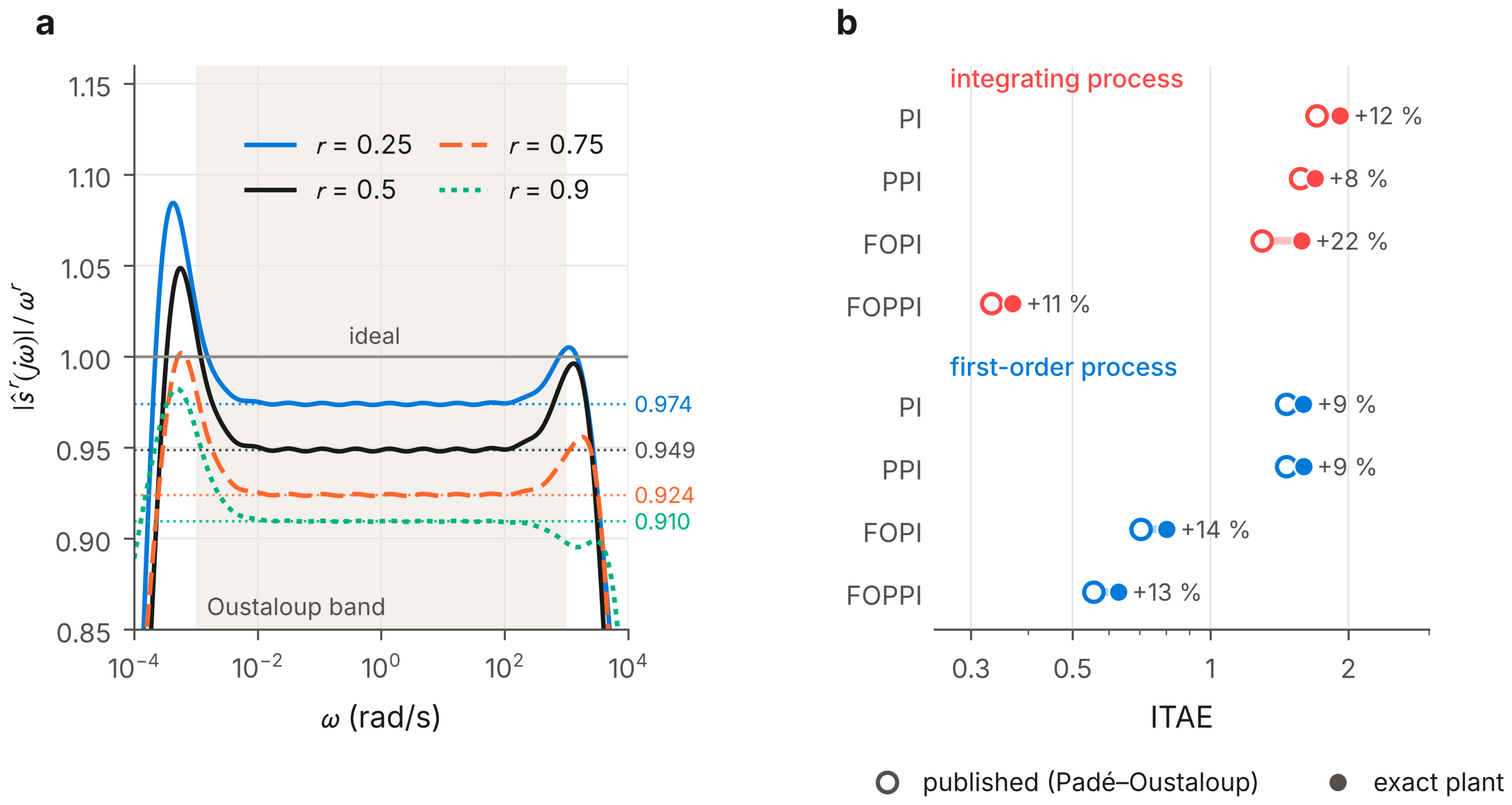
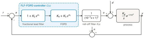
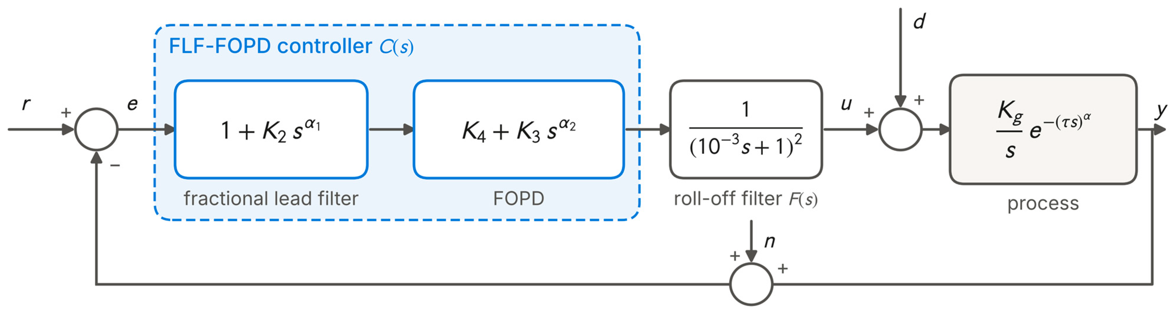
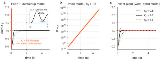
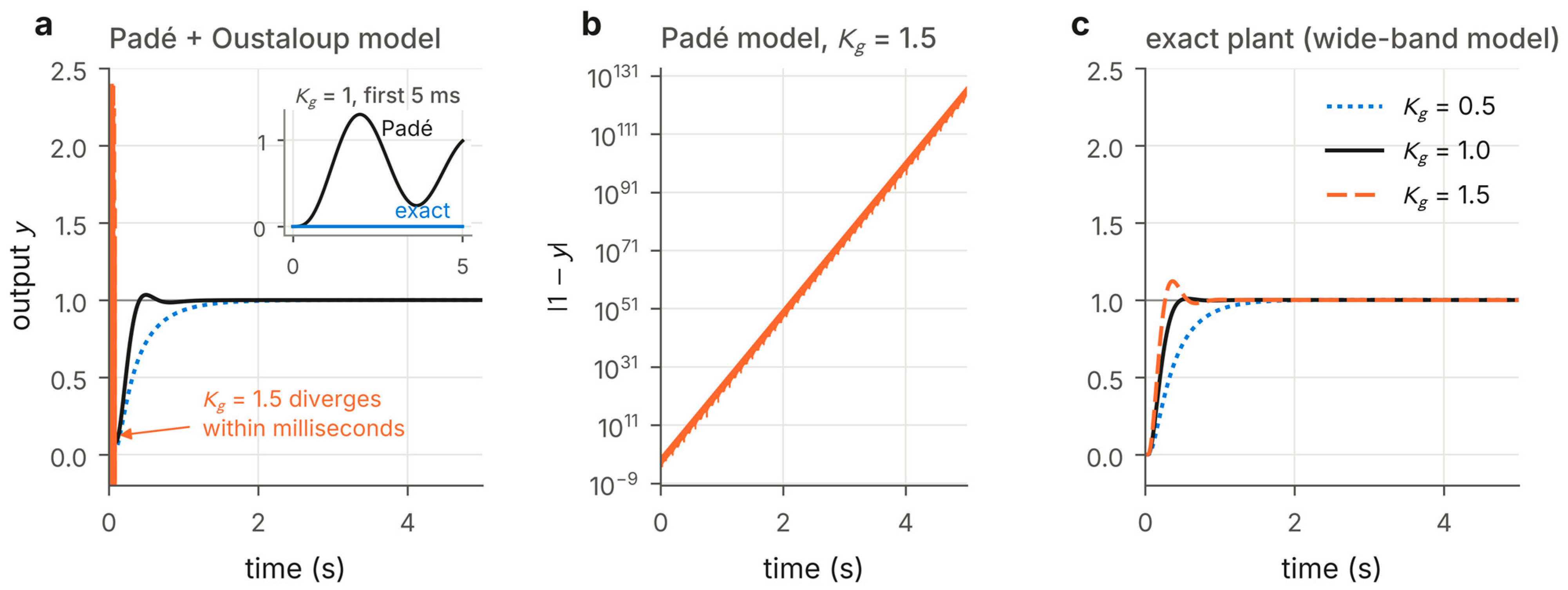
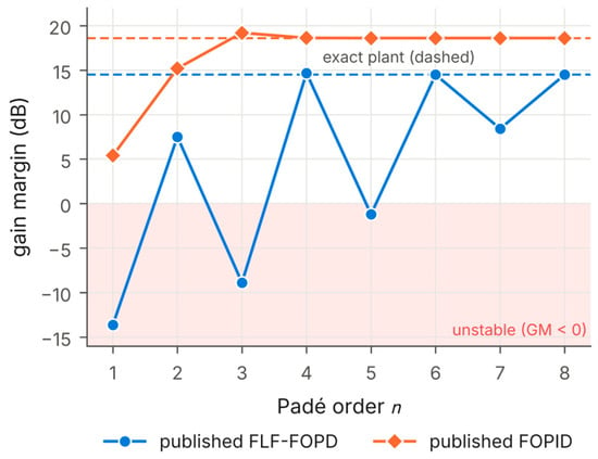
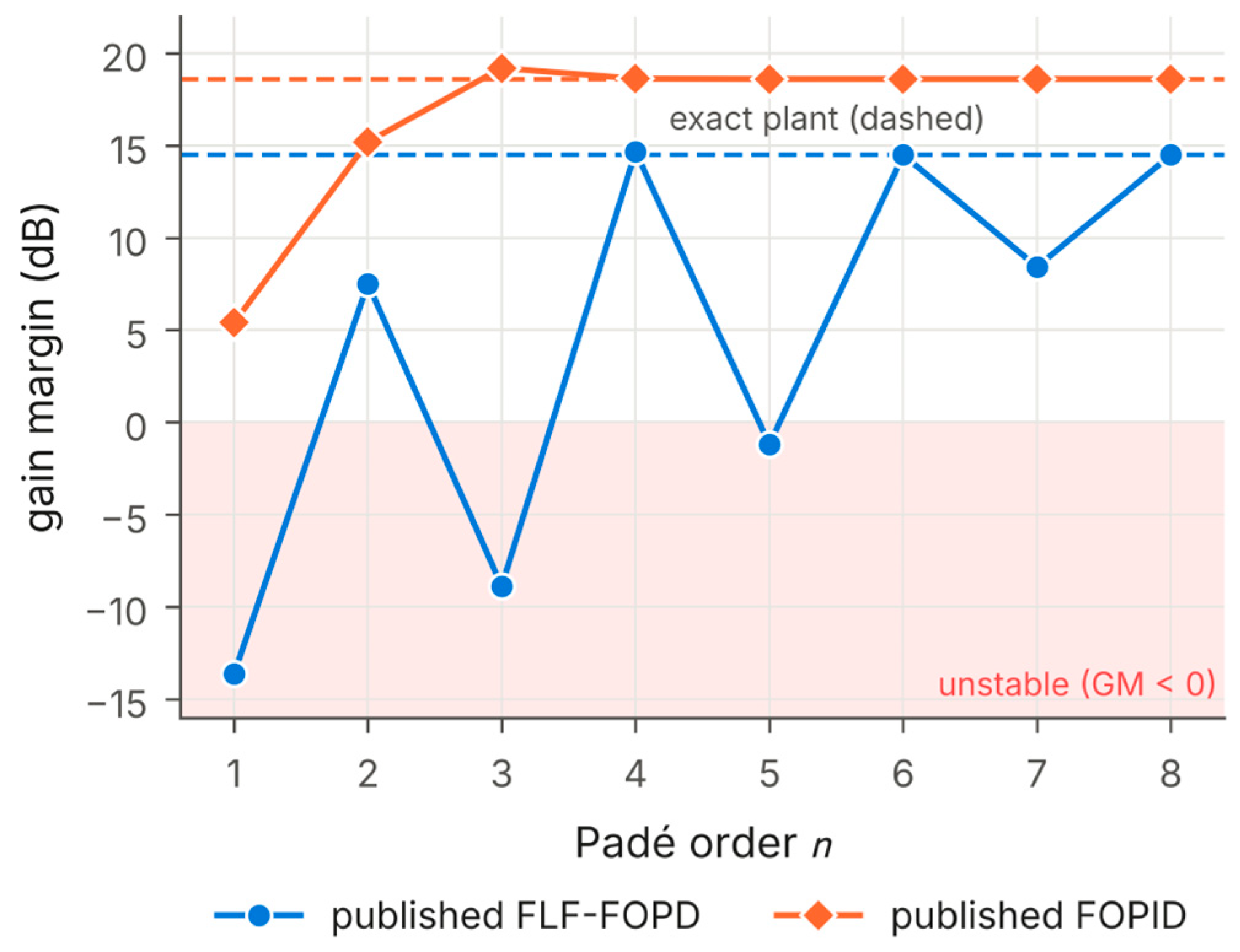
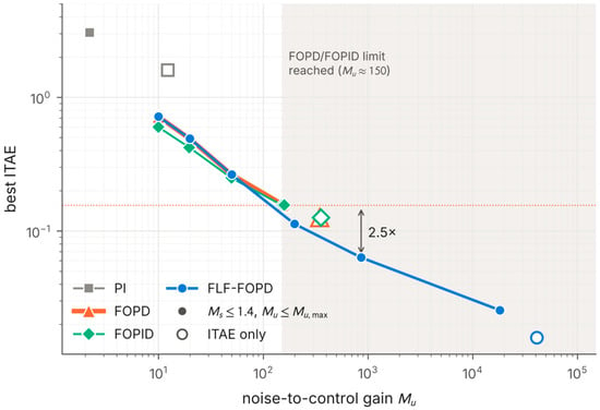
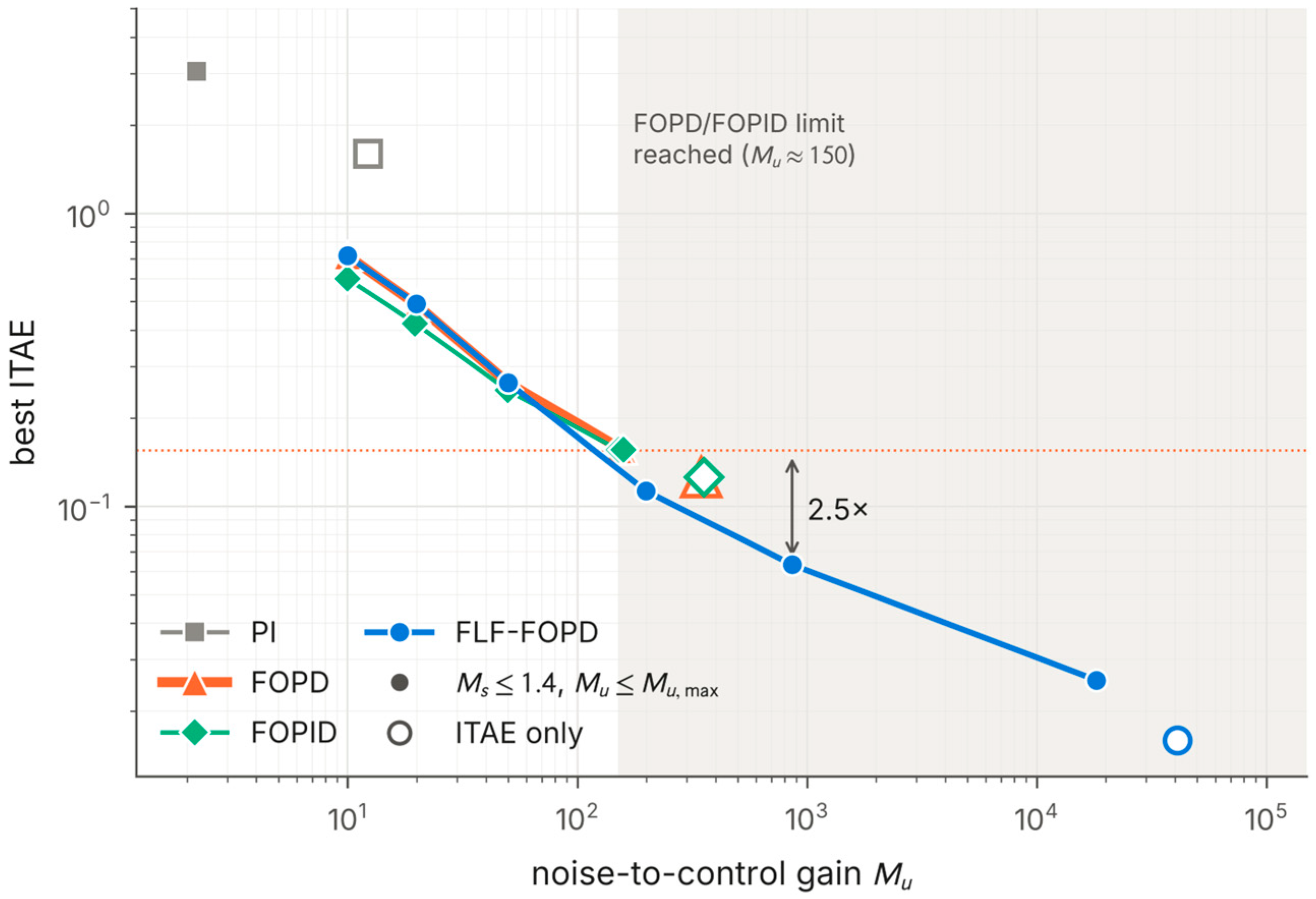
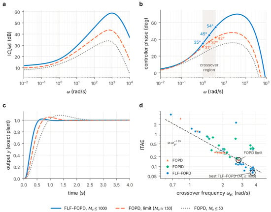
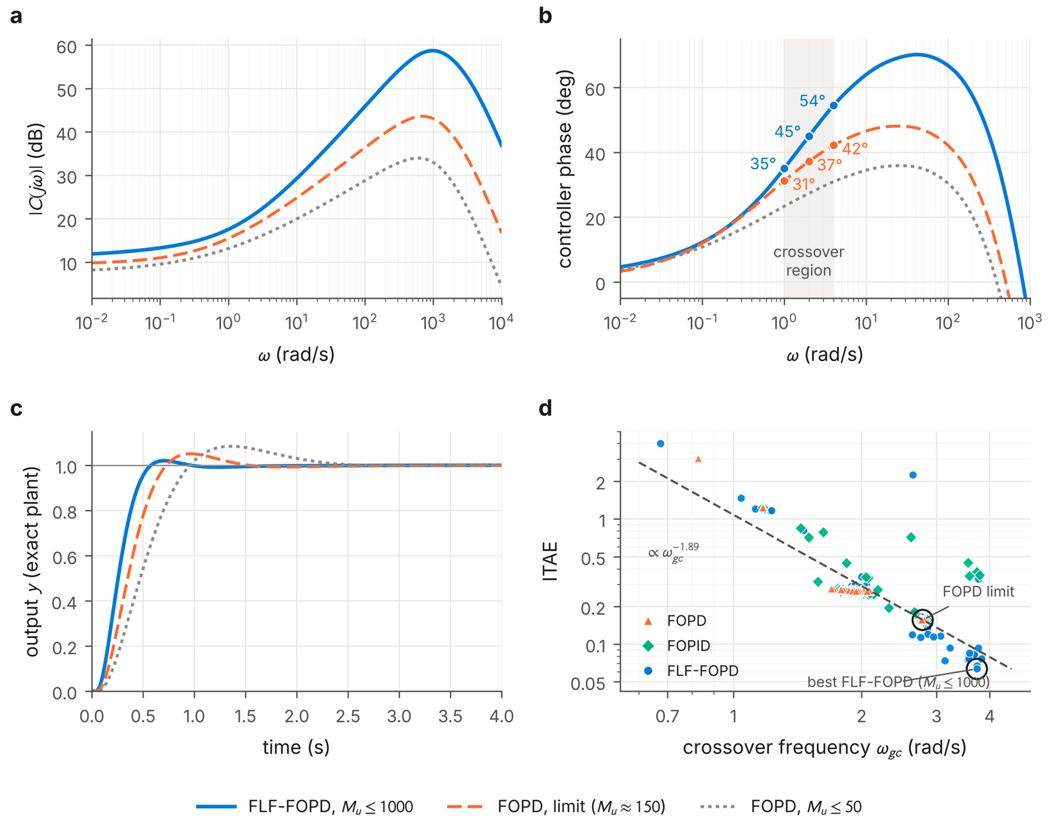

Disclaimer/Publisher’s Note: The statements, opinions and data contained in all publications are solely those of the individual author(s) and contributor(s) and not of MDPI and/or the editor(s). MDPI and/or the editor(s) disclaim responsibility for any injury to people or property resulting from any ideas, methods, instructions or products referred to in the content. |
© 2026 by the authors. Licensee MDPI, Basel, Switzerland. This article is an open access article distributed under the terms and conditions of the Creative Commons Attribution (CC BY) license.