


Abstract
This paper investigates stability and complete synchronization of distributed-order fractional nonlinear dynamical systems (DONDSs) with a constant time delay. For the continuous Caputo distributed-order model, a Laplace-transform resolvent approach gives the sufficient incremental small-gain condition under stated well-posedness and resolvent assumptions. The resolvent requirements are verified for scalar damping , for which the criterion reduces to , and for symmetric positive-definite A, for which is sufficient; well-posedness remains a separate hypothesis. For the finite multi-term model, the corresponding condition is . A conditional history-space generalized Wright Lyapunov criterion is also established, with decay described through a scalar multi-term relaxation function and its generalized Wright series representation subject to additional inversion conditions. We develop an Adams product integration predictor–corrector method, examine contraction of its endpoint corrector, and compare it with backward-Euler convolution quadrature and a fully implicit Adams endpoint. Finite multi-term Liu and financial systems illustrate the framework, accompanied by numerical studies of order distributions, delays, control gains, perturbations, and parameter interactions. Finally, an active control construction cancels nonlinear and delayed mismatch terms under ideal full state and exact model assumptions, leaving a stable linear distributed-order synchronization error system.
1. Introduction
Distributed-order nonlinear dynamical systems (DONDSs) provide a flexible framework for representing memory and hereditary effects that may involve a spectrum of fractional orders rather than a single fixed order. Fractional-order (FO) and distributed-order (DO) models have been used in biological, physical, and engineering applications [1,2,3,4,5,6,7,8]. These systems are particularly relevant in applications such as viscoelastic materials, anomalous diffusion, and control theory, where the dynamics are influenced by a spectrum of time scales and memory effects [9,10,11].
One of the critical challenges in the analysis of distributed-order (DO) systems is ensuring stability in the presence of nonlinearities and delays. Classical fractional stability theory includes Mittag-Leffler Lyapunov methods for nonlinear fractional systems [12], while delayed fractional systems have been treated through frequency-domain bounds, Razumikhin-type arguments, and related delay-dependent techniques [13,14,15]. Distributed-order stability has been studied in its own right [16,17]; numerical analysis for multi-order and distributed-order equations has been developed, for example, by Diethelm and Ford [18,19]. Delay distributed-order equations have also been investigated numerically [7]. Accordingly, we do not claim that delayed fractional or distributed-order analysis is new as a topic; the narrower point is that the particular combination used here—a continuous distributed-order resolvent criterion, its finite multi-term counterpart, a history-space generalized Wright criterion, and cancellation-based synchronization for delayed nonlinear systems—is comparatively less represented in one framework.
Synchronization of distributed-order chaotic systems has received substantial attention. Active-control, Lyapunov, linear feedback, and adaptive strategies have been developed for several distributed-order models [5,20,21]. The additional presence of an explicit time delay changes both the stability analysis and the numerical treatment, which motivates the delayed formulation considered here.
In this work, we consider a DONDS with a constant time delay
where , , , , and are continuous. The decomposition isolates the linear damping matrix A because A enters the transform-side resolvent , whereas f and g are treated as present-state and delayed Lipschitz perturbations in the small-gain estimate. The initial history is equipped with the norm
Throughout the paper, denotes the Euclidean norm for vectors and its induced spectral norm for matrices unless stated otherwise.
Definition 1.
Let satisfy almost everywhere and . With the fixed initial time (lower terminal) , the Caputo distributed-order derivative is defined by [17]
Thus, the operator in (1) is a weighted superposition of Caputo derivatives having the same lower terminal 0.
Remark 1
(Fixed lower terminal and memory). The lower terminal is part of the fractional operator, and is kept fixed at the initial time throughout this paper; it is not reset at , controller switching times, or numerical time steps. If a problem starts at a general time , the corresponding operator is
and changing changes the retained history as well as the resulting dynamics in general. This point is important for fractional systems with switching or piecewise inputs; for example, see [22,23]. In the present delayed model, the time origin is fixed at 0, while the prescribed history on supplies the delayed state before the evolution starts.
Remark 2.
Definition 1 is formulated for absolutely continuous-order distributions with density . A single-order Caputo model can be recovered as a singular limiting case by replacing the density with the Dirac measure . Such a Dirac measure is not itself an density, and will only be used below as a formal limiting case.
The main contributions are as follows. First, we provide a resolvent small-gain criterion for the continuous delayed distributed-order model and a separate finite multi-term counterpart. Second, building on the generalized Wright framework of [20], we formulate a conditional history-space Lyapunov criterion: if a functional satisfies the stated trajectory regularity, coercivity, and distributed-order decay inequality, its decay is controlled by the scalar multi-term relaxation kernel. Third, we formulate and diagnose an Adams product integration discretization, including the corrector contraction issue, an independent BE-CQ comparison, and a fully implicit endpoint variant. Finally, we place the classical cancellation-based active control mechanism in the present delayed distributed-order/finite multi-term setting, provide the exact cancellation assumptions, and quantify the sensitivity, control effort, and parameter effects numerically. The novelty of the synchronization result is not the cancellation principle itself but its transparent integration with the two distributed-order stability levels and the documented numerical limitations.
Relative to [20], the generalized Wright result is best interpreted as a history-space criterion applicable to the delayed model when a suitable can be verified. In the synchronization application, the chosen quadratic functional is instantaneous because the controller cancels the delays from the error equation. The resolvent criterion is complementary and genuinely retains the delayed state in the convolution estimate, although its sufficient small-gain constant is independent of the delay due to the supremum norm bound.
Table 1 summarizes the scope of the cited neighboring results along with the distinct roles of the results established here; the comparison is deliberately limited to the assumptions and methods relevant to this manuscript.
Table 1.
Comparison of assumptions, methods, and results with representative neighboring studies.
The rest of this paper is organized as follows: Section 2 gives the basic definitions and midpoint approximation; Section 3 develops continuous and finite multi-term resolvent stability criteria; Section 4 presents the conditional history-space generalized Wright stability criterion; Section 5 formulates the numerical discretization and reports the manufactured solution refinement test; the finite multi-term Liu and financial illustrations appear in Section 6; Section 7 develops the synchronization result and examples; and Section 8 concludes the paper.
2. Definitions and Preliminaries
This section presents the fundamental definitions of DO and FO derivatives together with the special function identities and auxiliary inequalities used below [9,17,25,26].
Standing Assumptions and Scope
For convenience, the principal hypotheses used later are collected here. The continuous-order stability result assumes a non-negative and nontrivial density , global Lipschitz bounds on the nonlinear terms, a well-posed admissible solution class, and the invertibility, boundedness/decay, and -kernel conditions stated in Assumption 1. The finite multi-term results use ordered orders and non-negative coefficients, with zero coefficients omitted; the finite resolvent theorem uses Assumption 2. The generalized Wright Lyapunov theorem additionally requires the scalar trajectory and the Caputo terms appearing in to possess the regularity and common Laplace transformability stated in Theorem 3. The numerical experiments use uniform grids with commensurate delays . The midpoint formula is used only when approximating a specified integrable density. The Liu/financial coefficients introduced later coincide algebraically, for , with midpoint values of the formal function ; however, this function is not integrable at . Those coefficients are treated as a prescribed finite discrete order measure, not as a quadrature of an density. These hypotheses are restated at the points where they are used to ensure that the scope of each result remains clear.
Definition 2.
For a function and order ν satisfying , the left-sided Riemann–Liouville fractional integral with the same lower terminal 0 is
Definition 3.
For any positive integer n satisfying , the Caputo FO derivative of with lower terminal 0 is
If g and its derivatives satisfy the usual exponential-order hypotheses required for the Laplace transform, then Equation (4) gives
The operator on the left of (5) is exactly the same Caputo operator as in (4); in particular, its lower terminal remains 0.
Definition 4
([25]). The two-parameter Mittag-Leffler function is given by
The Laplace transform of the function is
where is defined by
For parameters , the generalized Wright function is defined by
whenever the series converges. From this definition and (8),
Lemma 1
([9]). Let . Whenever the series below converges, the following expansion holds:
where denotes the multinomial coefficient ([26], Ch. 24). A convenient sufficient condition for the underlying geometric expansion at a given transform point s is
indeed, (11) is precisely the condition that the ratio of the lower-order part of the denominator to its two highest-order terms have modulus less than one before applying the geometric and multinomial expansions. For Laplace inversion, a useful sufficient contour condition is that for some Bromwich line ,
Under (12), the transform-side geometric series is uniformly absolutely convergent on that line. Term-by-term Bromwich inversion is then used only when the usual domination needed to interchange summation and inversion is also satisfied. For the positive coefficients used in the relaxation problem below, the contour inequality is not an additional restrictive parameter condition; it holds on every sufficiently far-right Bromwich line. Indeed, writing with and ,
while the numerator is at most . Hence, uniformly on ,
For signed or complex coefficients, such a positivity argument is unavailable, and the contour condition must be checked separately.
For the midpoint discretization, we additionally assume that the density w admits a continuous representative on (or is piecewise continuous with the quadrature nodes away from its discontinuities), so that pointwise sampling is meaningful. Let
and define the midpoint orders and quadrature coefficients by
Thus, . If a sampled coefficient vanishes, the corresponding term may be omitted. Whenever division by the highest-order coefficient is used below, the terms are relabeled so that . We denote the corresponding m-term approximation by
Every term has the same fixed lower terminal 0. To preserve the compact notation used in the subsequent formulas, we write from this point onward; no change of lower terminal is implied by this abbreviation. If the map is sufficiently smooth, the midpoint rule converges to the distributed-order integral as . Accordingly, the quadrature-discretized form of (1) is
Equation (15) is also meaningful as a finite multi-term model with coefficients prescribed directly, without an underlying integrable density. For the Liu and financial illustrations, and coincide formally with the midpoint values of . However, as this formal function is not integrable at , the coefficients are not interpreted as a quadrature of any density; they directly define a finite discrete order measure.
Lemma 2
(Quadratic Caputo inequality with the initial term explicit). Let with , and let . With the fixed lower terminal 0, for every ,
Consequently,
If , integration over the order gives
and the same inequality holds for the finite non-negative sum defined in (14).
Proof.
From the Caputo definition,
Since , the integration by parts is performed first on , where . Continuity at the initial point and give as , while implies , and hence as . Letting and yields (16). Both terms on its right-hand side are non-negative. This proof accommodates the usual integrable fractional startup singularity in and also shows where the initial value enters; no assumption is required for this particular inequality. The importance of retaining the correct initial value and lower terminal in fractional identities has been emphasized in [27,28]. □
Remark 3
(Role of non-negative order weights). The assumption is used when integrating the scalar Caputo quadratic inequality over the order as well as in the complete monotonicity arguments for the scalar resolvent kernels. The abstract resolvent theorems require the stated invertibility and kernel assumptions, but do not prove those properties for signed weights; therefore, signed weights are covered only if those resolvent assumptions are independently verified, and we do not perform any such verification.
3. Resolvent Stability of Continuous and Multi-Term Delayed Systems
We first state a resolvent criterion directly for the continuous distributed-order problem in (1), then derive the corresponding result for the midpoint-discretized system in (15). This avoids using the numerical quadrature as a surrogate for a continuous-order stability theorem.
For the continuous model, define the following for :
and, whenever is invertible,
We call a global solution admissible for the resolvent argument if it is of exponential order and if the distributed-order derivative may be interchanged with the Laplace transform on some common half-plane . The transform identity is required only on that half-plane; the time-domain variation-of-constants formula then follows by uniqueness of the Laplace transform. Under global Lipschitz bounds, exponential-order estimates are standard once the problem is represented as a locally integrable Volterra equation. General existence, continuation, resolvent, and Paley–Wiener frameworks for Volterra equations are given in [29]. We nevertheless retain well-posedness as an explicit hypothesis here rather than claiming that alone is sufficient.
Assumption 1.
There exist such that for all and all ,
The continuous problem in (1) is well-posed in a class of admissible global solutions. For , is invertible; is bounded with as ; and is locally integrable with
Theorem 1
(Continuous small-gain criterion).
Under Assumption 1, if
then (1) is globally incrementally asymptotically stable in the history norm. More precisely,
and for every pair of admissible histories. If, in addition, is an equilibrium, then the zero solution is globally asymptotically stable.
Proof.
Let x and y be two admissible solutions, set , and let denote their history difference. With and , the Laplace transform of the distributed-order error equation gives
Hence,
Writing and , the history contribution for yields
where
The resolvent assumptions imply and
Therefore, for ,
which gives a uniform history-norm stability bound because . In particular, v is bounded on . Set
Fix and choose such that for all . In the first convolution, split the integral at . The contribution from tends to zero, since v is bounded there and
while the remaining contribution is asymptotically bounded by . For the delayed convolution, split at ; its early part again vanishes by the tail of , whereas for one has . Since , taking upper limits in the error inequality gives
Letting yields ; since , , and hence . Comparing with the zero equilibrium gives global asymptotic stability when is an equilibrium. □
Corollary 1
(Scalar-damping case).
Assume that with , is non-negative and nontrivial, and the continuous problem is well-posed in the admissible class of Theorem 1. Suppose that the Lipschitz bounds in Assumption 1 hold. Then, the resolvent conditions in Assumption 1 are satisfied automatically and
Consequently, if
then the system in (1) is globally incrementally asymptotically stable. If is an equilibrium, it is globally asymptotically stable.
Proof.
For ,
Taking the principal branch , if , then and for every ,
Because and , it follows that , and hence that on , so is invertible there. Moreover, is a complete Bernstein function, and the complete-Bernstein/Stieltjes implications used below are standard; see Bazhlekova [30]. Hence, is a Stieltjes function and its inverse Laplace transform is non-negative. Likewise, the scalar relaxation function with transform is completely monotone. Thus, , , , and . Since , monotone convergence in its Laplace transform gives
because as . Therefore, under (21), and Theorem 1 applies. □
Corollary 2
(Symmetric positive-definite damping matrix). Suppose , let , and let be non-negative and nontrivial. Assume the well-posedness and Lipschitz hypotheses of Theorem 1. Then, the resolvent kernels satisfy Assumption 1 and
Consequently, the explicit sufficient condition
implies global incremental asymptotic stability; if zero is an equilibrium, it is globally asymptotically stable.
Proof.
Choose an orthogonal diagonalization , where each . Since is a complete Bernstein function, for every , the function is Stieltjes. Its inverse Laplace transform is non-negative and has integral
The scalar relaxation kernel with transform is completely monotone, bounded, and tends to zero. In the eigenbasis, and are diagonal with entries and the corresponding relaxation kernels. Moreover, if , then
The inverse Laplace transform of the right-hand side is non-negative, since it is a non-negative multiple of the convolution of two non-negative kernels; thus, . Because is itself an eigenvalue of the symmetric matrix A, the spectral norm satisfies , not merely an upper bound. Therefore
The relaxation entries are bounded and decay to zero, so the remaining kernel conditions hold. The result now follows from Theorem 1. □
Remark 4
(Beyond symmetric damping). Corollary 2 supplies a directly verifiable non-scalar matrix class. For a general non-normal A, positivity and simultaneous diagonalization are lost, so a bound depending only on cannot be asserted. The abstract theorem remains applicable whenever is invertible and the associated matrix Volterra resolvent belongs to ; frequency-domain/Paley–Wiener criteria of the type developed for matrix Volterra equations in [29] provide a route for verifying those assumptions on a case-by-case basis.
Remark 5.
Theorem 1 is a stability result for the continuous distributed-order equation itself; it does not require passage to the limit . The midpoint theorem below is a separate counterpart that is finite-dimensional in order, and convergence of , , and to their continuous analogues is a distinct approximation question.
Proposition 1
(Finite multi-term well-posedness).
Fix with and . Suppose that f is continuous in t and globally Lipschitz in its state variable uniformly in t, that g is globally Lipschitz, and that . Then, the multi-term delayed problem in (15) has a unique global continuous solution in its Volterra formulation on every finite time interval. Whenever the usual regularity required for the Caputo derivatives is available, this Volterra solution is equivalent to the differential formulation (15).
Proof.
After applying the fixed-lower-terminal Riemann–Liouville integral , the equation takes the weakly singular Volterra form displayed later in (46), with the linear term included in the instantaneous right-hand side. On a sufficiently short interval, the associated Volterra operator is a contraction in the supremum norm, since every kernel with is locally integrable and the full right-hand side is globally Lipschitz in the present and delayed states. The prescribed history supplies the delayed term before . Repeating the same contraction argument on successive intervals gives uniqueness and continuation, while the global Lipschitz estimate gives a Volterra–Gronwall bound on each finite interval and so excludes finite-time blow-up. Standard contraction, continuation, and weakly singular Volterra estimates of precisely this type are developed in Brunner ([31], Chs. 4 and 6); applying those estimates to (46) yields the asserted global Volterra solution. We state this proposition at the level of the Volterra solution; equivalence with the Caputo differential form is invoked only under the additional regularity specified in the statement. □
For the Laplace transform argument below, the difference of any two global solutions also has exponential order; indeed, the global Lipschitz bounds applied to the Volterra difference equation give a weakly singular Gronwall estimate of the form for suitable . Hence, e, F, and G are Laplace-transformable on a common right half-plane . The transform step in Theorem 2 is understood on that half-plane; Assumption 2 is stronger in requiring the finite resolvent itself to be well-defined for .
We now turn to the finite midpoint model. Let x and y be two solutions. Their initial histories satisfy
Set
Then,
where
Assumption 2.
The common Lipschitz bounds on f and g stated in Assumption 1 hold with constants . In addition, for , define
and assume that is invertible. Define the resolvent kernels
Assume that is bounded and as . Assume also that is locally integrable on and that
The local integrability formulation allows for the weak singularity at the origin that is typical of fractional resolvent kernels.
Theorem 2
(Resolvent small-gain criterion).
Suppose that Assumption 2 holds and
Then, the m-term system in (15) is globally incrementally asymptotically stable with respect to the history norm: for every , there exists independent of the particular pair of solutions, such that
and the two solutions are incrementally attractive for every pair of initial histories . In particular,
If, in addition, is an equilibrium, i.e., for all , then the zero solution is globally asymptotically stable.
Proof.
Taking the Laplace transform of (22) and using the Caputo transform formula gives
Hence, by (24) and the convolution theorem,
For , the delayed difference is determined by the initial histories, whereas for it equals . Therefore, with and ,
where the last integral is understood as zero when and
Assumption 2 implies that b is bounded. Moreover, the history term in (30) tends to zero because it is bounded by for , and this tail integral vanishes when . Together with , this gives . Since ,
Let . From (29),
Hence, for every ,
Set
Then, (31) gives . Hence, given , choosing (with the conclusion immediate if ) proves global incremental stability in the history norm. In particular, the error is bounded on . Let . Fix and choose such that for . In the first convolution of (29), the contribution from tends to zero because v is bounded there and
The remaining part is bounded asymptotically by . The delayed convolution is treated in the same way after splitting at . Therefore, taking the upper limit in (29) gives
Letting yields . Since , , which proves (27). The uniform estimate in (31) together with attractivity then proves global incremental asymptotic stability. If is an equilibrium solution, the same estimate with gives Lyapunov stability of the zero solution in the history norm, while (27) gives global attractivity; hence, the zero solution is globally asymptotically stable. □
Remark 6
(Why the small-gain bound is delay-independent). The condition in Theorem 2 is a sufficient and generally conservative bound. In the convolution estimate, the delay enters as the shifted error ; for , this shift does not enlarge the supremum bound on the error, while the kernel contributes only through . This norm estimate discards phase and frequency information, so the resulting sufficient condition has no explicit τ. By retaining the delay in a characteristic equation or a delay-dependent Lyapunov–Krasovskii estimate, delay-dependent criteria can be less conservative; thus, independence of this particular bound from τ does not mean that the actual dynamics are insensitive to delay.
Numerical Illustration of the Small-Gain Criterion
To illustrate Theorem 2 independently of the nonlinear Liu and financial illustrations considered later, consider the scalar delayed multi-term problem
where
Here, , while and have global Lipschitz constants . In this scalar positive-coefficient case,
The function is a Stieltjes function, so its inverse Laplace transform is non-negative. Moreover, is precisely the scalar multi-term relaxation function ; by Lemma 3, it is completely monotone and tends to zero. Consequently,
Thus, the resolvent assumptions and the small-gain condition of Theorem 2 are verified for this example. We solved (32) using the predictor–corrector method of Section 5, using , one corrector iteration, and the three constant histories:
Figure 1 shows the convergence of all three trajectories to the equilibrium, while Figure 2 shows the decay of the pairwise trajectory differences, numerically illustrating the incremental attractivity asserted by Theorem 2.
Figure 1.
Solutions of (32) generated from three distinct constant histories. The numerical parameters are , , , and one corrector iteration.
Figure 2.
Pairwise trajectory errors for (32). Their decay illustrates incremental attractivity under the verified small-gain value .
4. Generalized Wright Stability
The generalized Wright concept used here is adapted from the non-delayed framework in [20]. We formulate it as a conditional history-space criterion on . The delay enters the estimate substantively only when V genuinely depends on and satisfies the hypotheses below. In the synchronization application, V is instantaneous because the controller cancels the delayed mismatch, so no delay-dependent Lyapunov–Krasovskii estimate is claimed.
We next formulate a Lyapunov-functional criterion for the m-term approximation. Let , and define the scalar relaxation function by
Its Laplace transform is
For positive coefficients and orders , is the standard multi-term fractional relaxation function. For the explicit representation only, zero coefficients are omitted, repeated orders (if any) are combined, and the remaining terms are relabeled so that
This ordering is required for the series representation below, but not for the Laplace transform definition in (34).
To display its generalized Wright representation, set
For , let . For a multi-index with , define
Whenever the contour condition in (12) (with and ) holds on a Bromwich line and the corresponding term-by-term inversion is justified by the usual domination condition stated in Lemma 1, inversion of (34) yields
Using (9), the last factor may be written equivalently as
The Laplace transform formula (34) is the primary definition. The time-domain series (36) is invoked only when the transform-side expansion of Lemma 1 satisfies the stated contour convergence condition and the interchange of summation with Bromwich inversion is justified; none of the stability results below requires (36) outside of these conditions.
Lemma 3.
Assume , not all zero, and . Then, for every , the inverse Laplace kernel
is non-negative, while is completely monotone, satisfies , and obeys
Proof.
The required complete-monotonicity properties are standard for discrete distributed-order relaxation equations; see Bazhlekova [30]. Set
Then, is a complete Bernstein function. Hence, is a Stieltjes function, so . Moreover,
is a Stieltjes function, which implies that is completely monotone. Its non-negativity and complete monotonicity guarantee the existence of a finite limit at infinity. Since as , the Abelian final-value relation gives
□
Definition 5
Theorem 3.
Let be a continuous Lyapunov functional. Along a solution, set , with . Here,
Thus, the Caputo derivatives act on the scalar trajectory ; we do not invoke a Fréchet derivative of V on the history space or a fractional chain rule for V. Assume , that the Caputo derivatives in the above finite sum exist almost everywhere and are locally integrable, and that v together with these Caputo terms is Laplace-transformable in a common right half-plane (for example, under the corresponding exponential-order bounds). A genuinely history-dependent functional is admissible whenever its composition with the solution satisfies the following requirements. Assume that there exist such that for every history ,
and
where for . Then,
Consequently, the zero solution is generalized Wright stable and asymptotically stable, since by Lemma 3.
Proof.
Remark 7
(Scope of the delay dependence). Theorem 3 is a conditional history-space criterion: the delay enters through the segment only when the chosen functional genuinely depends on that segment. The instantaneous quadratic choice is a special case, and does not necessarily create a delay-dependent estimate. We do not claim a general Lyapunov–Krasovskii construction for (15); in particular, for moving-window terms such as , the Caputo derivative is nonlocal and cannot be replaced by the classical Leibniz rule, so verifying (41) requires a separate fractional-delay argument. Razumikhin-type approaches provide an alternative route for genuinely delay-sensitive criteria; see, e.g., [14]. A history-dependent V is admissible in Theorem 3 only when satisfies the stated local absolute continuity and common Laplace transformability assumptions and when (41) can actually be verified.
Remark 8
(Synchronization-error example). A concrete instance is the synchronization error in Section 7. For the finite multi-term model, the controller gives
with . Choose the history functional
Then, in (40), and Lemma 2 gives
Hence, Theorem 3 applies with and yields the explicit decay estimate
Thus, the generalized Wright criterion is realized concretely by the error dynamics arising from delayed drive–response systems after exact active-control cancellation.
5. Numerical Method
The time variable t in all numerical illustrations denotes dimensionless model time, with no physical unit such as days or seconds assigned. The Liu and financial examples are benchmark models without a specified physical time calibration, and the remaining examples are mathematical test problems. For a dimensional distributed-order operator, coefficients of fractional derivatives of different orders would need compatible order-dependent physical units; no such scaling is prescribed here. Accordingly, the horizontal axes of the time-dependent figures are labeled “Time t (dimensionless)”; the phase portraits display state coordinates instead of time.
We formulate an Adams–Bashforth–Moulton product integration predictor–corrector discretization for the midpoint-discretized delayed system. To keep the formulas compact while remaining consistent with (15), define
We keep the notation distinct throughout this section in order to avoid conflating the original nonlinearity f with the full instantaneous term.
With the midpoint orders and coefficients defined in (13), assume (after omitting zero terms if necessary) that the largest retained coefficient satisfies . Then, this system is
Applying the fixed-lower-terminal Riemann–Liouville integral and using
we obtain the Volterra form
where .
Let , and assume for simplicity that with an integer . The grid is extended to by . Hence, the delayed value at is always ; for , this value is supplied by the initial history. If is not an integer, an interpolation rule for the delayed argument must be specified separately. Define
Following the fractional Adams product-integration approach [24,32,33,34], the predictor at is
For the corrector, let
Then
If additional corrector iterations are desired, set , and for , define
where
The product integration coefficients are
The numerical implementation is determined by the order nodes , coefficients , time step h, delay index r, and the number of corrector iterations . These quantities are part of the computational specification of the scheme. The present work does not claim a general global convergence order for this multi-term delayed discretization; establishing such an error theorem, including its dependence on the smallest order gaps and on solution regularity near , is left for future analysis. The manufactured solution test below is used only as a refinement check.
- Compact Algorithm and Cost
For : (i) read the delayed grid value from the prescribed history or the accepted solution; (ii) form the m history convolutions in (47); (iii) compute ; (iv) evaluate the endpoint right-hand side and perform corrector updates from (49) or solve the implicit endpoint (53); and (v) accept and append its right-hand-side value to the history. Direct convolution requires arithmetic operations over N steps. The state history requires storage while precomputing all order-dependent convolution weights requires up to additional storage. Short-memory truncation reduces cost at the price of a controlled memory approximation, while sum-of-exponentials, FFT/block convolution, or other fast-history techniques can reduce the quadratic-time bottleneck; however, these accelerations are not used in the reported runs.
The scheme is related to the classical fractional Adams predictor–corrector method [24,32] as well as to multi-order formulations [18] and distributed-order numerical analysis [19]. For a smooth single-order problem, the classical one-corrector Adams method has the familiar order under the corresponding regularity assumptions. Multi-term equations can possess startup singularities and several competing order gaps, meaning that single-order rate does not constitute a convergence theorem for (45); therefore, Table 2 is interpreted empirically.
Table 2.
Mesh refinement results for the manufactured delayed multi-term problem (54).
5.1. Fully Implicit Adams Product Integration Endpoint
The finite corrector iteration in (49) need not converge. This issue can be diagnosed at a fixed time step with the past values held fixed. Define
For the scalar current-state term with and a positive commensurate delay, successive endpoint iteration errors satisfy . Thus, this fixed-point iteration is contractive exactly when . More generally, if the instantaneous term is Lipschitz with constant and so that the delayed endpoint is already known, the corrector map has the sufficient contraction factor
For zero delay, a current-state contribution from g adds . This clarifies the dependence on step size: contains and , so a small highest-order coefficient can indeed make the endpoint iteration restrictive, although this is a condition on the iteration at only a single step. At and , with , this factor is for the manuscript coefficients, for uniform midpoint weights, for , and for . More iterations cannot cure the non-contractive cases.
We also solve the Adams–Moulton endpoint equation fully implicitly. Let and
The new endpoint is the solution of
This follows from the same product integration rule as (49); subtracting cancels its constant-history contribution exactly. This is a fully implicit variant, distinct from a prescribed finite number of predictor–corrector iterations. In the scalar affine case, its denominator is strictly positive. For the full-state synchronization example below, the current-state Jacobian is triangular with negative diagonal entries , so its implicit endpoint is also uniquely solvable. These observations establish endpoint solvability only for the tested examples.
The implicit equations were solved numerically and checked against an absolute infinity-norm residual tolerance of at every step. The maximum residual in the added experiment suite was . In the contractive manufactured case, the result agreed with 60 iterations of (49) within . The single integer-order limit also reproduced the trapezoidal rule within .
5.2. Manufactured Solution Accuracy Test
To assess the time discretization in Section 5 independently of the nonlinear application examples, we consider a scalar finite multi-term problem for which the exact solution is prescribed. We use the same 20 orders and coefficients employed later in the Liu and financial illustrations:
and define
with history for . The forcing term is chosen as
Since
the exact solution of (54) is
The predictor–corrector method was applied on with two corrector iterations. The step sizes all satisfy , so the delayed value is taken directly from the accepted mesh point. We measure the maximum grid error
and the observed refinement rate
The results are reported in Table 2.
The error decreases under every mesh refinement, indicating progressively better agreement with the manufactured solution for this test. However, the observed rates drift downward rather than approaching a clear asymptotic value, so reporting one definitive convergence order would be misleading. The rates in Table 2 are reported only as an empirical refinement check for this fixed finite multi-term problem; no formal convergence order is inferred.
5.3. Independent Time Integrator and Corrector Iteration Comparison
For an independent check, we also used first-order backward-Euler convolution quadrature (BE-CQ) for the Caputo terms, following Lubich [35]. The weights satisfy and , applied to in the Caputo history-shift formula. Nonlinear implicit steps were solved to residual tolerance . All delays were commensurate with the time grid. Table 3 compares both methods on the manufactured problem with the manuscript’s 20-term coefficients.
Table 3.
Maximum manufactured solution errors for ABM with two corrector iterations and backward-Euler convolution quadrature (BE-CQ).
Increasing the number of corrector updates greatly improves this particular manufactured solution result. The error falls from approximately with the predictor alone to approximately after four updates. This behavior indicates a substantial endpoint iteration contribution to the error at the tested step size. Still, it must not be extrapolated to non-contractive endpoint maps, where additional Picard updates can instead amplify an error; the refinement data remain empirical, and do not establish a general convergence order.
5.4. Order Quadrature and Delay Distribution Study
We use the continuous density and exact solution on , with . The forcing is constructed from the continuous distributed-order derivative. Midpoint models with are compared against an solution on the same BE-CQ grid () and with the same continuous forcing. The order quadrature error is ; the time error is measured separately against the exact solution using forcing matched to each finite model. Doubling the number of order nodes reduces the difference from the fine-m reference by approximately a factor of four, consistent with midpoint quadrature behavior for the smooth density considered here. At the fixed time step, the temporal error is much larger and can conceal this improvement in an overall error measure. This distinction is why order quadrature refinement must not be confused with convergence of the complete continuous-order discretization. The order-quadrature and time-discretization errors are summarized in Table 4.
Table 4.
Separated order quadrature and time discretization errors for the uniform order density using BE-CQ with .
With , , and , we also vary the delay and use the normalized density shapes , , and . Table 5 gives the maximum errors against the same exact solution using BE-CQ.
Table 5.
Manufactured solution maximum errors for delay and order density sweeps using BE-CQ.
The manufactured density comparison in Table 5 shows a consistent ordering of the observed errors: the low-order-heavy density yields the smallest values and the high-order-heavy density the largest. The modest variation with delay concerns the numerical error for this constructed exact solution; it does not imply that increasing the delay improves the stability of the underlying dynamics. In this setting, the order distribution changes the discrete memory operator, and hence the error behavior.
A stability limitation of the displayed ABM discretization was also exposed. For , uniform midpoint weights, , , and one corrector iteration, the manufactured trajectory exceeded by and subsequently overflowed, while BE-CQ remained finite. Accordingly, the density and order convergence results above use BE-CQ; they are not presented as validation of ABM for all admissible weights. The finite iteration method’s stable parameter range requires further analysis; the non-contractive endpoint iteration is addressed by the fully implicit variant in Section 5.1 and Section 5.5.
5.5. Validation of the Fully Implicit Variant
We repeated the previously non-contractive density tests using (53). All computed trajectories remained finite over the stated intervals. Table 6 reports temporal refinement with forcing matched to each finite model, , , and . The rates are empirical and do not imply a general convergence theorem.
Table 6.
Maximum manufactured solution errors using the fully implicit Adams endpoint.
Across all four tested coefficient families, the fully implicit endpoint yields decreasing errors under temporal refinement. More importantly, it remains finite in the manufactured cases for which the finite Picard iteration was non-contractive. Solving the endpoint equation directly addresses the observed iteration failure in these runs, although it does not imply a general nonlinear stability theorem.
Comparison with the fully implicit endpoint in Table 6 suggests that the endpoint iteration error may contribute to this changing refinement pattern: on a common grid, the implicit solution is substantially more accurate and its observed rates are more regular. This comparison motivates checking the corrector convergence separately from mesh refinement, without attributing the drift exclusively to the finite corrector.
We also repeated the uniform-density quadrature study on the same grid using the fully implicit endpoint and . Table 7 distinguishes the fixed-grid difference between order discretizations, with common continuous-order forcing, from the temporal error measured using forcing specific to the finite model. The former estimates the sensitivity of the computed solutions to order discretization, but does not provide an exact decomposition of the continuum error. The rate in Table 7 refers only to the difference from the reference. The finite-model time error column uses a different m-term operator and its matched forcing in each row; therefore, its decrease as m increases is a change in the time discretization error constant for those different finite models, not an order quadrature convergence rate.
Table 7.
Order quadrature difference and finite-model temporal error using the fully implicit Adams endpoint. The reported rate is computed from the difference-from- column only.
The fully implicit delay sweep covered for all four coefficient families. Every tested run remained finite, with maximum errors of order . For a fixed coefficient family, the maximum error is unchanged across the tested delays because it occurs within the initial time layer, that is, before the delayed argument leaves the prescribed history. This does not make the full trajectory delay-insensitive; errors at later times do vary with . Rather than establishing a delay-independent error bound or isolating a dynamical delay effect, the sweep checks the implementation and boundedness of the fully implicit method for these manufactured examples. The earlier BE-CQ results provide a separate numerical comparison.
6. Numerical Illustrations for Finite Multi-Term Liu and Financial Models with Time Delay
6.1. Liu-Type Finite Multi-Term Illustration
We begin with the delayed FO Liu model introduced in [36]:
For the numerical illustration, we use the following finite multi-term counterpart of the delayed distributed-order Liu model:
For the numerical computations, the finite multi-term model uses orders:
and the positive coefficients
These coefficients specify the finite multi-term model. For , they coincide formally with midpoint values of , but that function is non-integrable at ; hence, the coefficients are not interpreted as quadrature weights for an density. For transparency, their total mass is ; the highest-order coefficient contributes of this mass, and the coefficients span approximately decimal orders (). Thus, this particular finite measure is strongly concentrated near the largest retained order and should not be interpreted as a generic distributed-order density. Normalizing the weights to unit mass would multiply the effective right-hand side coefficients by , and hence define a different finite model. For this reason, we keep the stated coefficients but supplement them with the density/order/delay comparisons in Section 5.4 and Section 5.5 as well as the synchronization sensitivity study in Section 7.4. The predictor–corrector implementation uses and one corrector iteration. For the Liu model, we take
with the constant history
The finite multi-term Liu system is integrated on . Since , every delayed term at is evaluated from the accepted grid state , with the prescribed constant history used before . Figure 3 is generated from this implementation of Model (57). The phase portraits are reported as qualitative illustrations of the nonlinear dynamics. The baseline delay is only one time step, and is treated as a reproducible parameter choice rather than evidence of a substantive delay effect. A direct study of the same Liu model with larger delay is reported immediately below. To keep the numerical claims tied to the documented computations, no Lyapunov exponent values are reported for this example.
Figure 3.
Phase portraits of the finite 20-term Liu model: (a) projection onto the -plane and (b) projection onto the -plane, with , , , , and the model parameters specified in the text. The constant initial history is for .
To document the behavior of the Liu computation when the delay parameter is changed, we repeated the same finite 20-term model with the same coefficients, constant history, time step , and one corrector iteration, but with over the common finite horizon . All five computed trajectories remained finite, but their pointwise separations from the baseline increased markedly. The magnitude of such separation alone cannot distinguish a response to changing the delay from sensitivity to tiny disturbances in a chaotic computation. As a numerical sensitivity control, we also repeated the baseline calculation after adding only to the first component of the constant history, with no delay change. On the logarithmic scale in Figure 4, the curves for the changed delay lie many orders of magnitude above this control during the early part of the integration (before the control itself undergoes strong chaotic amplification). The perturbed-history control grows to the same broad scale as the changed-delay separations, by about and thereafter, so late-time pointwise distances are no longer delay-specific. Thus, the figure supports an early-time response to the delay change while also showing why long-time pointwise trajectory differences in this chaotic calculation cannot isolate a delay effect by themselves. A stronger delay-specific dynamical conclusion would require attractor-level or statistically converged comparisons together with solver- and precision-sensitivity controls.
Figure 4.
Finite-horizon trajectory divergence in the Liu computation, shown on a logarithmic vertical scale. Solid curves show for . The dashed control repeats but perturbs the first component of the constant history by only . The changed-delay separations dominate the control by many orders of magnitude at early times; after the control is chaotically amplified (around in this run), all pointwise separations enter a comparable broad scale and are no longer delay-specific. Here, , , and we use a single corrector iteration.
Remark 9.
The finite operator may equivalently be viewed as the distributed-order derivative associated with the discrete order measure . If only one term with coefficient is retained, the equation has the form . Dividing by gives a single-order Caputo Liu model of the same algebraic form (with the right-hand side coefficients rescaled by ) of the type studied in [36]. This interpretation is distinct from the -density formulation in Definition 1.
6.2. Financial Finite Multi-Term Illustration
Wang et al. [37] investigated the FO financial model with time delay as follows:
For the numerical illustration, we use the finite multi-term counterpart
For the financial model, we use the same 20-term coefficients, , one corrector iteration, , and
The constant history is
The financial system is integrated directly with delay index , so every delayed term at is evaluated from the accepted grid state (and from the prescribed constant history when ), as specified in Section 5. Figure 5 is regenerated from this implementation. As in the Liu example, the phase portrait is presented as a qualitative illustration without quoting Lyapunov exponent values. The delay is only five time steps, and is treated as part of this reproducible portrait, not as evidence of a substantial delay effect. The direct sensitivity experiment with larger delay is limited to the Liu model as a representative chaotic delay diagnostic; no corresponding larger-delay financial sweep is claimed. The method-oriented delay checks in Section 5.4 and Section 5.5 and the synchronization sensitivity study in Section 7.4 address separate numerical questions, and are not used to infer a delay effect for the financial model. The endpoint quantities for the common manuscript coefficients and used in Figure 3, Figure 4, and Figure 5 are and . Thus, the corrector iteration contraction condition becomes whenever a bound for the instantaneous endpoint map is available, which represents an endpoint iteration diagnostic.
Figure 5.
Phase portraits of the finite 20-term financial model: (a) projection onto the -plane and (b) projection onto the -plane, with , , , , and initial history for .
Remark 10.
As in Remark 9, the finite operator in (59) corresponds to a discrete order measure. If one Caputo term is retained, dividing the equation by the positive coefficient gives a single-order financial model of the same algebraic form, with all right-hand side coefficients (including the constant source term) scaled accordingly, as in [37]. The finite multi-term computation reported here should be interpreted as a multi-order counterpart, not as a quadrature experiment for a specified continuous density.
7. Synchronization Between Two Different DO Dynamical Systems with Time Delay
Definition 6.
Consider the following two DONDSs with time delay:
- Drive system:where f is nonlinear, is the drive delay, and is the drive state.
- Response system:where g is nonlinear, is the response delay, is the response state, and is the control input.
Remark 11.
If, as a singular limiting case, the order distribution is replaced by the Dirac measure , then the synchronization problem reduces to synchronization between two fractional-order dynamical systems with time delays [38]. Formally taking the boundary limit (outside the standing assumption ) recovers the corresponding integer-order synchronization problem [39].
Remark 12.
If , the systems have no time delay. The synchronization problem reduces to the standard synchronization of DONDSs [20].
Remark 13.
If f and g are linear functions, the synchronization problem can be solved using linear control techniques such as state feedback or observer-based control.
Remark 14.
Complete synchronization of DONDSs with time delays may have applications in secure communication, financial modeling, and complex networks.
7.1. Complete Synchronization Between Two Different DONDSs with Time Delays
Theorem 4.
Consider the drive and response systems in (60) and (61). Suppose that both use the same distributed-order operator from Definition 1, and assume that for the prescribed initial histories, the drive system and controlled response system under the law below both admit global solutions in the class for which the distributed-order derivatives and Laplace transform identities used in the proof are valid. Let . Then, the active control law
where , achieves complete synchronization.
Proof.
Subtracting the drive equation from the controlled response equation and substituting (62) gives the exact cancellation
Thus, no nonlinear mismatch remains in the synchronization-error dynamics. Since K is symmetric positive definite, write , where Q is orthogonal and with . Setting yields the following decoupled equations:
Define
For each component, the Laplace transform is
For a non-negative and nontrivial density, the corresponding distributed-order relaxation function is non-negative and completely monotone; see Bazhlekova [30]. Hence, the limit exists. Since
and as by dominated convergence, the Abelian final-value relation for a function possessing a finite limit gives
Therefore, for every i, and consequently .
For the midpoint-discretized model, the same conclusion follows directly from Lemma 3; alternatively, with , Lemma 2 gives
and Theorem 3 yields the same decay estimate. Thus, complete synchronization is achieved for both the continuous distributed-order model and its midpoint approximation. □
Remark 15
(Scope and novelty of the synchronization result). Theorem 4 is an exact-cancellation active-control result. Once (62) is substituted, the nonlinearities and both delays disappear from the error equation (63); consequently, the ideal synchronization decay is delay-independent and follows from the scalar distributed-order relaxation analysis. This cancellation principle is classical in active-control synchronization, including distributed-order work such as [20,21]. The contribution here is not a new cancellation mechanism but its formulation alongside the continuous/finite delayed distributed-order stability framework, together with explicit information assumptions and numerical tests of discretization, perturbation, control effort, and parameter sensitivity.
Remark 16
(Information required by the active controller). The cancellation in Theorem 4 is an ideal full-state feedback result. Implementing the law as written requires access to the current drive and response states and to the delayed states appearing in both models, together with a common time base and the same distributed-order operator. Measurement noise, parameter uncertainty, communication loss, and partial-state observation are not included in the theorem or the numerical example. Robust, adaptive, and observer-based versions are natural extensions in future work.
7.2. An Example
As an illustrative example, we apply the synchronization scheme developed in Section 7.1. We consider the finite multi-term Liu model (57) as the drive system and the finite multi-term financial model (59) as the response system. The midpoint counterpart of Theorem 4 applies because the same finite operator is used in both systems. The controlled response system is given by
where is the vector of control inputs.
Applying the finite multi-term counterpart of Theorem 4, the control functions in (62) are derived as follows:
where for represents the synchronization errors and the gains satisfy . Hence, , consistent with the positive-definiteness hypothesis of Theorem 4. Equations (64) and (65) give an analytical controller derivation for the Liu drive/financial response pair; no numerical Liu-to-financial synchronization simulation is reported in this subsection. The computed synchronization illustration is the separate two-dimensional example in Section 7.3.
The following reproducible two-dimensional post-substitution experiment illustrates the error decay predicted by Theorem 4, although does not independently verify the analytical cancellation.
7.3. A Reproducible Synchronization Experiment
Consider the two-dimensional delayed drive system
with constant history on . The controlled response system is chosen as
with constant history on the common history interval . Hence, both histories are defined on and . The finite operator uses
Choose . From Theorem 4, the control inputs are
Substitution of (68) into (67) gives exactly
For the numerical illustration, the closed-loop equations were integrated in their post-substitution form after the algebraic cancellation in (69), using the predictor–corrector scheme of Section 5, , and one corrector iteration. The stored x and y components are retained so that can be plotted. Because the nonlinear and delayed mismatch has already been removed analytically before time-stepping, Figure 6 and Figure 7 illustrate the decay of the resulting closed-loop error dynamics; they do not constitute an independent numerical verification of the cancellation itself. At , this post-substitution integration gives
Figure 6.
Drive and controlled-response components for the reproducible synchronization experiment with , , drive delay , response delay , and .
Figure 7.
Absolute synchronization errors for the reproducible experiment with , , and . Both components decay toward zero, in agreement with Theorem 4.
The decreasing componentwise errors are consistent with the two damped equations in (69). The stronger damping of the second component affects the reduced model directly, but neither curve tests the cancellation mechanism under imperfect model information.
The same post-substitution predictor–corrector baseline states used in Figure 6 and Figure 7 were used to reconstruct the control inputs from (68). Figure 8 reports the two control-input components and . The figure shows a pronounced control transient associated with the initial drive–response mismatch, followed by a much smaller input magnitude as the error decays. Evaluating (68) at gives and , with . The peak control norm is , compared with an RMS norm of and a terminal norm of . The contrast describes the distribution of control effort over this finite test; it does not establish actuator feasibility or robustness under uncertainty.
Figure 8.
Control inputs and their Euclidean norm reconstructed from the post-substitution single-corrector predictor–corrector baseline states, with , , , drive delay , and response delay . The components and may be signed, whereas the Euclidean norm is non-negative. The plot illustrates the control effort associated with the analytically canceled closed-loop model; it is not an independent numerical test of cancellation.
7.4. Synchronization Sensitivity to Delay, Order Measure, and Control Gain
We performed additional post-substitution closed-loop simulations using BE-CQ and evaluated from the computed states. In this separate two-dimensional test, the swept parameter is the delay in the drive equation (the argument in (66)); the response delayed terms have already been removed by the algebraic substitution. With the manuscript order coefficients, , and , the drive-delay sweep gave in every case to numerical precision. This delay-independence is built into the analytically reduced error equation after cancellation, making it a consistency check on the implementation as opposed to an independent numerical confirmation of the cancellation; the drive trajectories themselves still depend on delay.
For , so that , the terminal error decreases as shown in Table 8. The BE-CQ calculation remained finite through the largest tested gain. In contrast, ABM with and exceeded by ; this is a discretization limitation, not instability of the controlled continuous system.
Table 8.
Effect of the smallest control matrix eigenvalue on the terminal synchronization error using BE-CQ.
The monotone gain trend in Table 8 is consistent with stronger damping in the analytically-reduced linear error dynamics. It should not be read as proof that the finite-corrector ABM method remains stable as gains increase; the high-gain divergence above illustrates precisely the distinction between controlled-system damping and endpoint-iteration convergence.
Additional BE-CQ sweeps used coefficient multipliers , uniform-density order counts , and the three explicit densities (uniform), (low-order-heavy), and (high-order-heavy). At the fixed terminal time, uniformly increasing the order coefficients increases the remaining error for this reduced equation. This coefficient-scale sweep is an algebraic consistency check rather than an independent physical sensitivity; multiplying every by a common factor c in is equivalent to replacing K by . Thus, scales correspond to effective gains and their terminal errors coincide with the entries for , 1, and , respectively, in Table 8. The order count sweep changes the terminal error only slightly (approximately –), indicating weak sensitivity to further order node refinement in this particular uniform density experiment. The shape of the order distribution has a larger effect: the low-order-heavy density gives a larger remaining error (about ) than the uniform density (about ), while the high-order-heavy density gives a smaller one (about ). These results represent finite-horizon properties of the analytically reduced linear error equation.
To probe sensitivity to imperfect cancellation, we also added a bounded deterministic residual to the two response/control channels,
so that the numerically realized error equation becomes . This perturbation is intended as a reproducible aggregate model of small measurement/implementation error; it is not a stochastic noise model and does not constitute a robust control theorem. With , the manuscript coefficients, , , and , Table 9 reports the maximum perturbation-induced deviation from the unperturbed numerical error trajectory. Because exact cancellation leaves a linear error equation and enters additively, the perturbation-induced deviation is linear in for each fixed discretization up to roundoff. Indeed, is for BE-CQ and for the fully implicit Adams endpoint for every row of the table to the reported precision. Accordingly, this experiment measures the forced response of the linear numerical error equation; it should not be interpreted as evidence of nonlinear closed-loop robustness. All trajectories remained finite, and the two discretizations are closely consistent.
Table 9.
Sensitivity to a bounded residual controller perturbation .
7.5. A Compact Full-Factorial Sensitivity Check
To examine joint effects rather than only one-factor sweeps, we also performed a deterministic full-factorial BE-CQ study, following the general factorial design idea illustrated in [40]. The factors were for , , , and the drive-system delay . The response delay is absent from the post-substitution equations used in this factorial calculation. To make the comparison in m approximate the same continuous order distribution, we used the uniform density and midpoint weights rather than the strongly m-dependent illustrative coefficient formula used in the Liu/financial examples. The response was .
For each two-level factor, the reported effect is the mean response at the second listed level minus the mean response at the first listed level. The results indicate that the control gain is the dominant factor in the tested range; increasing it reduces the terminal error by a factor of approximately (Table 10). Refining the order grid or time grid has a much smaller effect on this response, and the drive delay factor has no observable effect because the delayed terms were already eliminated from the post-substitution error equation. While the comparatively small interactions suggest that these selected factors act nearly independently over the tested levels, the deterministic and unreplicated design only supports descriptive contrasts.
Table 10.
Main effects and largest interaction in the full-factorial synchronization study. Effects are contrasts in .
7.6. Fully Implicit Synchronization Checks
The full drive–response simulations were repeated using (53), with the same delay, coefficient scale, order count, density shape, and gain sweeps as above. Every state remained finite. For , the finite Picard iteration for the second error component has factor at . The fully implicit endpoint avoids this divergent iteration. When successively halving h from to , the terminal error changed only slightly and approached approximately . This agreement under refinement supports numerical consistency of the fully implicit solution in the previously problematic high-gain example, though it does not prove unconditional stability. The maximum absolute state was 2, attained in the initial data.
The implicit gain sweep in Table 11 is consistent with the independent BE-CQ comparison. The delay sweep again produced to the reported precision, as expected from exact cancellation. These finite-time checks address the previously failing numerical settings.
Table 11.
Fully implicit Adams endpoint: terminal synchronization error for , , , drive system delay , and manuscript coefficients.
8. Conclusions
This work has considered delayed distributed-order nonlinear dynamical systems at both the continuous-order and finite multi-term levels. For the continuous Caputo distributed-order equation, we establish a Laplace transform resolvent small-gain criterion for incremental asymptotic stability under stated well-posedness and resolvent-kernel assumptions. The midpoint approximation yields a finite multi-term system for which an analogous resolvent theorem and a conditional history-space generalized Wright Lyapunov functional criterion were developed. A delayed Adams–Bashforth–Moulton product integration discretization was formulated with consistent delay indexing and optional corrector iterations. The manufactured solution refinement study provides an empirical accuracy check, while a rigorous global convergence-order theorem is left for future work. Independent BE-CQ comparisons and separate order quadrature, delay, density shape, coefficient, control gain, and bounded controller perturbation studies are also reported. The finite-corrector ABM implementation becomes unbounded for some tested weights and gains. An endpoint iteration calculation identifies non-contractive cases, while a fully implicit Adams product integration variant resolves these failures in the repeated tests and exhibits mesh refinement. We do not claim a general time-discrete nonlinear stability and convergence theorem. For synchronization, the proposed active-control law cancels the nonlinear mismatch exactly, leaving a stable linear distributed-order error equation.
Taken together, the experiments separate three distinct numerical questions: refinement accuracy for a fixed model, contraction of the endpoint corrector, and the sensitivity of the reduced synchronization error to model parameters. The fully implicit endpoint improves the behavior of the tested non-contractive discretizations, while the cancellation-based control results remain analytically idealized. The figures and tables quantify these distinctions.
The numerical section uses a specified 20-term finite model. The Liu and financial illustrations are finite multi-term counterparts with fully reported order nodes, coefficients, model parameters, delays, histories, and time-stepping data. Their portraits are regenerated from implementations matching Models (57) and (59); for the financial model, the delay uses the exact mesh index .
The numerical discussion is restricted to the quantities and computational settings specified in the manuscript. A separate nonlinear delayed example is used to verify the finite resolvent assumptions; this gives the explicit small-gain value , while its trajectories demonstrate incremental attractivity. Finally, a fully specified two-dimensional drive–response experiment with is integrated in the post-substitution closed-loop form, illustrating the predicted decay of the synchronization errors. The cancellation itself is the preceding algebraic identity, and is not independently established by the numerical integration. A bounded residual perturbation study further quantifies finite-time sensitivity to imperfect cancellation for the tested numerical setting; thos is included as a diagnostic only, and is not a robust control theorem. Potential application settings include communication systems and financial dynamics; however, the examples presented here remain at the stage of mathematical illustrations.
- Limitations and Future Work
The global results rely on global Lipschitz perturbation bounds together with resolvent integrability or a sufficiently dominant positive damping matrix. They do not cover general local nonlinear stability. The finite m-term model and the continuous distributed-order model are analytically distinct, and only targeted smooth-density convergence studies in m are reported. A general convergence theorem for the delayed product integration method, especially for non-smooth startup behavior, remains open. The original Liu and financial portraits use small delays; in the additional larger-delay Liu computation, the changed-delay separations clearly exceed the history perturbation control during the early-time interval. By about , chaotic amplification brings the control to the same broad scale; consequently, we do not interpret late-time pointwise differences as an isolated delay effect. No general delay-dependent stability or bifurcation map is claimed. The synchronization theorem is an ideal exact-model/full-state cancellation result; mismatch, noisy measurements, partial observations, and communication effects require robust/adaptive/observer designs. Direct convolution also has cost and full-history memory. Natural extensions include local and delay-dependent stability, distributed or time-varying delays, rigorous convergence as , fast/short-memory convolution, robust synchronization, and broader factorial designs with additional weight parameters and replicated uncertainty scenarios that would allow for ANOVA quantification of both main effects and interactions.
Author Contributions
Conceptualization, T.A., A.S.A., and T.M.A.-E.; methodology, T.A., A.S.A. and T.M.A.-E.; formal analysis, T.A., A.S.A. and T.M.A.-E.; investigation, T.A., A.S.A. and T.M.A.-E.; writing—original draft preparation, T.A., A.S.A. and T.M.A.-E.; writing—review and editing, T.A., A.S.A. and T.M.A.-E. All authors have read and agreed to the published version of the manuscript.
Funding
This research received no external research funding.
Institutional Review Board Statement
Not applicable. This study did not involve humans or animals.
Informed Consent Statement
Not applicable.
Data Availability Statement
No external datasets were used or analyzed in this study. The numerical results were obtained through simulations using the model parameters and initial conditions specified here. For the common 20-term baseline model, the fractional-order nodes and coefficients are and , . For the Liu model, , , , , and , with constant initial history for . For the financial model, , , , and , with constant initial history for . For the two-dimensional synchronization example, , the drive and response delays are and , respectively, and the constant histories are and on . The remaining parameter choices, including the scalar stability example, manufactured solution test, sensitivity studies, time step sizes, integration intervals, and corrector iterations, are given in the corresponding sections, figures, and tables.
Acknowledgments
The researchers would like to thank the Deanship of Graduate Studies and Scientific Research at Qassim University (https://www.qu.edu.sa, accessed on 20 October 2026) for financial support (QU-APC-2026).
Conflicts of Interest
The authors declare no conflicts of interest.
References
- Caputo, M.; Mainardi, F. A new dissipation model based on memory mechanism. Pure Appl. Geophys. 1971, 91, 134–147. [Google Scholar] [CrossRef] [Scilit]
- Lorenzo, C.F.; Hartley, T.T. Variable order and distributed order fractional operators. Nonlinear Dyn. 2002, 29, 57–98. [Google Scholar] [CrossRef] [Scilit]
- Ganie, A.H.; Aljuaydi, F.; Ahmad, Z.; Bonyah, E.; Khan, N.; Alharthi, N.; Murtaza, S.; AlBaidani, M.M. A fractal–fractional perspective on chaotic behavior in 4D memristor-nonlinear system. AIP Adv. 2024, 14, 015135. [Google Scholar] [CrossRef] [Scilit]
- Ding, W.; Patnaik, S.; Sidhardh, S.; Semperlotti, F. Applications of distributed-order fractional operators: A review. Entropy 2021, 23, 110. [Google Scholar] [CrossRef] [Scilit] [PubMed]
- Abed-Elhameed, T.M.; Mahmoud, G.M.; Elbadry, M.M.; Ahmed, M.E. Nonlinear distributed-order models: Adaptive synchronization, image encryption and circuit implementation. Chaos Solitons Fractals 2023, 175, 114039. [Google Scholar] [CrossRef] [Scilit]
- Farhan, M.; Aljuaydi, F.; Shah, Z.; Alzahrani, E.; Bonyah, E.; Islam, S. A fractional modeling approach to a new Hepatitis B model in light of asymptomatic carriers, vaccination and treatment. Sci. Afr. 2024, 24, e02127. [Google Scholar] [CrossRef] [Scilit]
- Pimenov, V.G.; Hendy, A.S.; De Staelen, R.H. On a class of non-linear delay distributed order fractional diffusion equations. J. Comput. Appl. Math. 2017, 318, 433–443. [Google Scholar] [CrossRef] [Scilit]
- Abed-Elhameed, T.M.; Otefy, M.; Mahmoud, G.M. Dynamics of chaotic and hyperchaotic modified nonlinear Schrödinger equations and their compound synchronization. Phys. Scr. 2024, 99, 055226. [Google Scholar] [CrossRef] [Scilit]
- Podlubny, I. Fractional Differential Equations: An Introduction to Fractional Derivatives, Fractional Differential Equations, to Methods of Their Solution and Some of Their Applications; Academic Press: San Diego, CA, USA, 1999. [Google Scholar]
- Mainardi, F. Fractional Calculus and Waves in Linear Viscoelasticity: An Introduction to Mathematical Models; World Scientific: Singapore, 2022. [Google Scholar]
- Mahmoud, G.M.; Khalaf, H.; Darwish, M.M.; Abed-Elhameed, T.M. Synchronization and desynchronization of chaotic models with integer, fractional and distributed-orders and a color image encryption application. Phys. Scr. 2023, 98, 095211. [Google Scholar] [CrossRef] [Scilit]
- Li, C.; Chen, Y.; Podlubny, I.; Mittag. Leffler stability of fractional order nonlinear dynamic systems. Automatica 2009, 45, 1965–1969. [Google Scholar] [CrossRef] [Scilit]
- Chen, Y.Q.; Moore, K.L. Analytical stability bound for a class of delayed fractional-order dynamic systems. Nonlinear Dyn. 2002, 29, 191–200. [Google Scholar] [CrossRef] [Scilit]
- Chen, B.; Chen, J. Razumikhin-type stability theorems for functional fractional-order differential systems and applications. Appl. Math. Comput. 2015, 254, 63–69. [Google Scholar] [CrossRef] [Scilit]
- Birs, I.; Muresan, C.; Nascu, I.; Ionescu, C. A survey of recent advances in fractional order control for time delay systems. IEEE Access 2019, 7, 30951–30965. [Google Scholar] [CrossRef] [Scilit]
- Fernández-Anaya, G.; Nava-Antonio, G.; Jamous-Galante, J.; Muñoz-Vega, R.; Hernández-Martínez, E. Asymptotic stability of distributed order nonlinear dynamical systems. Commun. Nonlinear Sci. Numer. Simul. 2017, 48, 541–549. [Google Scholar] [CrossRef] [Scilit]
- Jiao, Z.; Chen, Y.-Q.; Podlubny, I. Distributed-Order Dynamic Systems: Stability; Springer: London, UK, 2012. [Google Scholar]
- Diethelm, K.; Ford, N.J. Multi-order fractional differential equations and their numerical solution. Appl. Math. Comput. 2004, 154, 621–640. [Google Scholar] [CrossRef] [Scilit]
- Diethelm, K.; Ford, N.J. Numerical analysis for distributed-order differential equations. J. Comput. Appl. Math. 2009, 225, 96–104. [Google Scholar] [CrossRef] [Scilit]
- Mahmoud, G.M.; Aboelenen, T.; Abed-Elhameed, T.M.; Farghaly, A.A. Generalized Wright stability for distributed fractional-order nonlinear dynamical systems and their synchronization. Nonlinear Dyn. 2019, 97, 413–429. [Google Scholar] [CrossRef] [Scilit]
- Mahmoud, G.M.; Farghaly, A.A.; Abed-Elhameed, T.M.; Aly, S.A.; Arafa, A.A. Dynamics of distributed-order hyperchaotic complex van der Pol oscillators and their synchronization and control. Eur. Phys. J. Plus 2020, 135, 32. [Google Scholar] [CrossRef] [Scilit]
- Hu, J. Studying the memory property and event-triggered control of fractional systems. Inf. Sci. 2024, 662, 120218. [Google Scholar] [CrossRef] [Scilit]
- Hu, J.-B.; Zheng, Z.; Ying, C.-T.; Li, S.-G.; Tan, P. The stability and oscillation analysis of fractional neural networks under periodically intermittent control from its response property. Inf. Sci. 2025, 716, 122241. [Google Scholar] [CrossRef] [Scilit]
- Diethelm, K.; Ford, N.J.; Freed, A.D. A predictor-corrector approach for the numerical solution of fractional differential equations. Nonlinear Dyn. 2002, 29, 3–22. [Google Scholar] [CrossRef] [Scilit]
- Miller, K.S.; Ross, B. An Introduction to the Fractional Calculus and Fractional Differential Equations; Wiley-Interscience: Hoboken, NJ, USA, 1993. [Google Scholar]
- Abramowitz, M.; Stegun, I.A. Handbook of Mathematical Functions: With Formulas, Graphs, and Mathematical Tables; Courier Corporation: North Chelmsford, MA, USA, 1965. [Google Scholar]
- Zhao, L. A note on “Cluster synchronization of fractional-order directed networks via intermittent pinning control”. Phys. A Stat. Mech. Its Appl. 2021, 561, 125150. [Google Scholar] [CrossRef] [Scilit]
- Zhao, L.; Chen, Y. Comments on “A novel approach to approximate fractional derivative with uncertain conditions”. Chaos Solitons Fractals 2022, 154, 111651. [Google Scholar] [CrossRef] [Scilit]
- Gripenberg, G.; Londen, S.-O.; Staffans, O. Volterra Integral and Functional Equations; Cambridge University Press: Cambridge, UK, 1990. [Google Scholar]
- Bazhlekova, E. Completely monotone functions and some classes of fractional evolution equations. Integral Transform. Spec. Funct. 2015, 26, 737–752. [Google Scholar] [CrossRef] [Scilit]
- Brunner, H. Collocation Methods for Volterra Integral and Related Functional Differential Equations; Cambridge University Press: Cambridge, UK, 2004. [Google Scholar]
- Diethelm, K.; Ford, N.J.; Freed, A.D. Detailed error analysis for a fractional Adams method. Numer. Algorithms 2004, 36, 31–52. [Google Scholar] [CrossRef] [Scilit]
- Bhalekar, S.; Daftardar-Gejji, V. A predictor-corrector scheme for solving nonlinear delay differential equations of fractional order. J. Fract. Calc. Appl. 2011, 1, 1–9. [Google Scholar]
- Wang, Z. A numerical method for delayed fractional-order differential equations. J. Appl. Math. 2013, 2013, 256071. [Google Scholar] [CrossRef] [Scilit]
- Lubich, C. Discretized fractional calculus. SIAM J. Math. Anal. 1986, 17, 704–719. [Google Scholar] [CrossRef] [Scilit]
- Bhalekar, S.; Daftardar-Gejji, V. Fractional ordered Liu system with time-delay. Commun. Nonlinear Sci. Numer. Simul. 2010, 15, 2178–2191. [Google Scholar] [CrossRef] [Scilit]
- Wang, Z.; Huang, X.; Shi, G. Analysis of nonlinear dynamics and chaos in a fractional order financial system with time delay. Comput. Math. Appl. 2011, 62, 1531–1539. [Google Scholar] [CrossRef] [Scilit]
- Wang, S.; Bekiros, S.; Yousefpour, A.; He, S.; Castillo, O.; Jahanshahi, H. Synchronization of fractional time-delayed financial system using a novel type-2 fuzzy active control method. Chaos Solitons Fractals 2020, 136, 109768. [Google Scholar] [CrossRef] [Scilit]
- Pyragas, K. Synchronization of coupled time-delay systems: Analytical estimations. Phys. Rev. E 1998, 58, 3067. [Google Scholar] [CrossRef] [Scilit]
- Shahin, R.; Hosteins, P.; Pellegrini, P.; Vandanjon, P.-O. A full factorial sensitivity analysis for a capacitated Flex-Route Transit system. In Proceedings of the 2023 8th International Conference on Models and Technologies for Intelligent Transportation Systems (MT-ITS); IEEE: Piscataway, NJ, USA, 2023; pp. 1–6. [Google Scholar] [CrossRef] [Scilit]
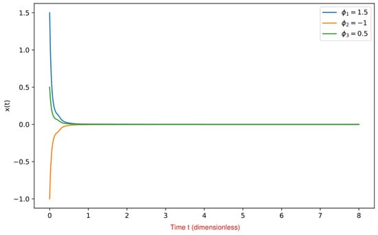
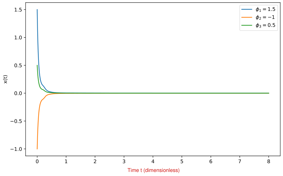
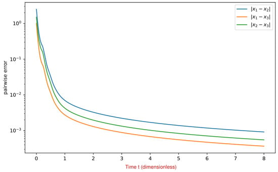
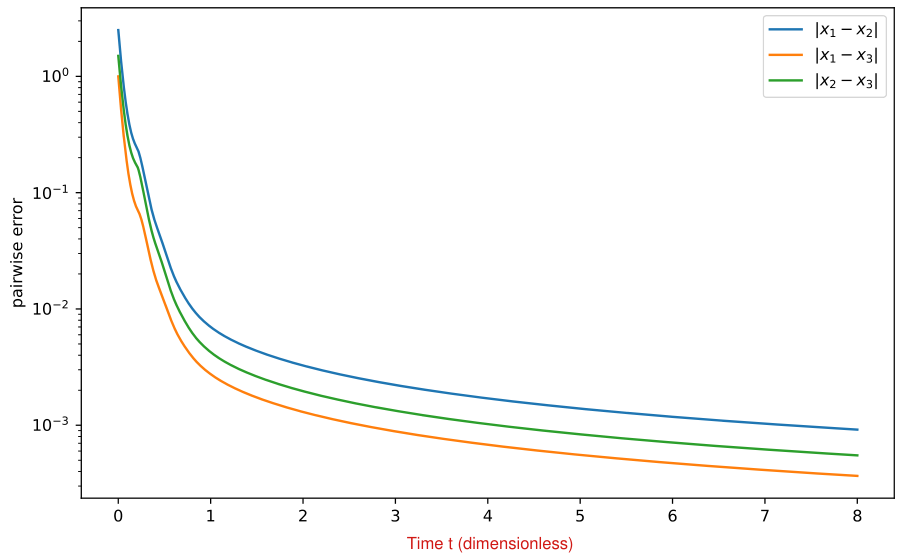
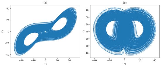
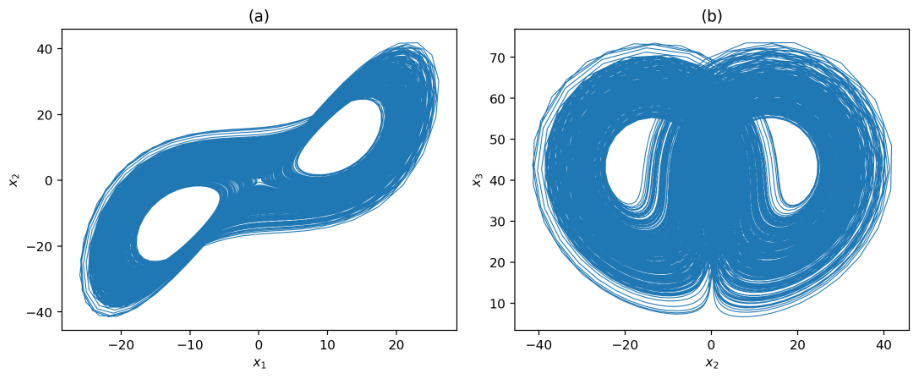
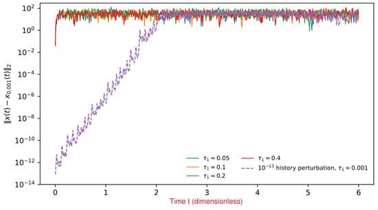
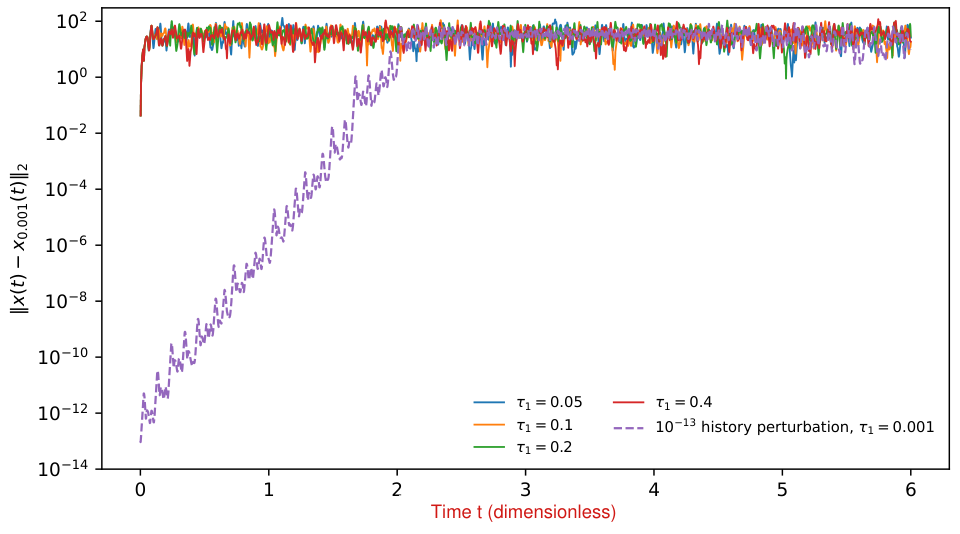
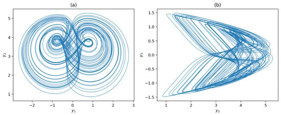
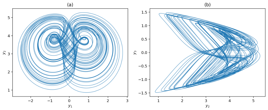
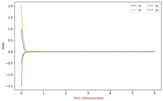
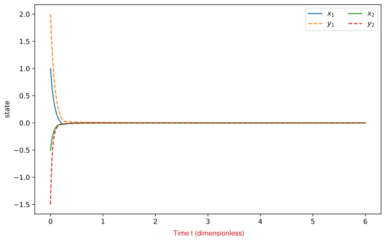
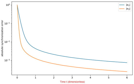
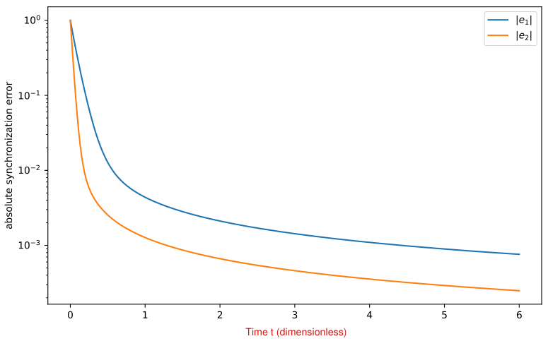
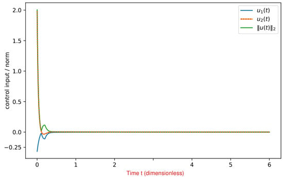
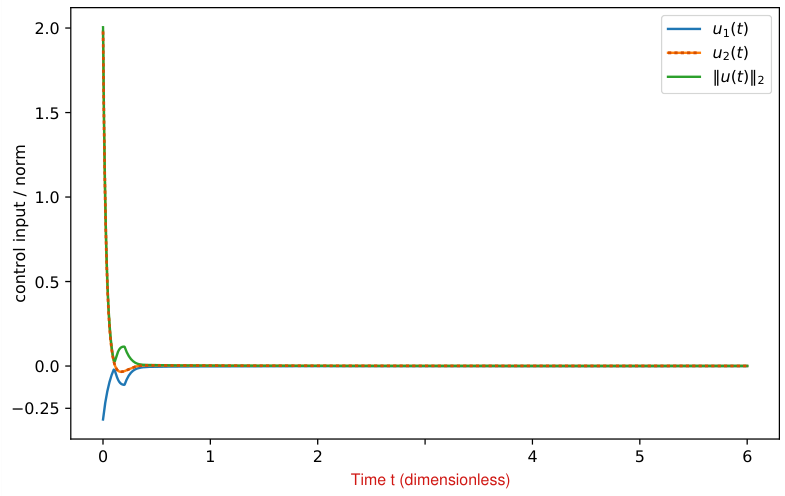

Disclaimer/Publisher’s Note: The statements, opinions and data contained in all publications are solely those of the individual author(s) and contributor(s) and not of MDPI and/or the editor(s). MDPI and/or the editor(s) disclaim responsibility for any injury to people or property resulting from any ideas, methods, instructions or products referred to in the content. |
© 2026 by the authors. Licensee MDPI, Basel, Switzerland. This article is an open access article distributed under the terms and conditions of the Creative Commons Attribution (CC BY) license.