


Abstract
Fractional differential equations and fractional-order chaotic systems are attractive for secure communications, but the nonlocal memory of the Caputo derivative makes their digital implementation costly, so iterative methods are preferred for developing digital implementations of physical systems. This paper characterizes seven members of the Lorenz family (Lorenz, Chen, Burke–Shaw, Liu, Shimizu–Morioka, Lü, and Yang) and implements them on an FPGA using the short-memory principle. Starting from rectangular (REC) and predictor–corrector (PC) product-integration rules, we derive incremental iterative forms with a finite memory window suited to digital hardware. Largest Lyapunov exponent maps and bifurcation diagrams over fractional order and memory duration identify chaotic regimes for the Caputo case that, to our knowledge, have not been reported; for most systems, they stabilize once the window exceeds about 2 s. On a Cyclone V FPGA with a common Q1.11.20 fixed-point format, each architecture lets you select any of the seven systems and a memory depth of 1–1000 samples without resynthesis. For a 2 s window, REC uses fewer resources (3258 ALMs, 60 DSP blocks), whereas PC, thanks to its larger time step, reaches a higher estimated state-generation rate (330,457 versus 291,839 state vectors/s). Finally, 8-bit pseudorandom sequences extracted from the Lorenz system (1 Gbit per architecture) pass NIST SP 800-22 and the TestU01 Rabbit, Alphabit, and BlockAlphabit batteries. In addition, we present numerical simulations and their digital implementation to validate the numerical schemes.
1. Introduction
Fractional calculus studies the differentiation and integration of non-integer order, where the order may be rational, real, or complex [1,2,3]. Its origins date back to a 1695 correspondence between Leibniz and L’Hôpital, in which they first proposed the concept of a fractional derivative [4]. Although fractional calculus remained primarily theoretical for centuries, Fractional-Order Systems (FOSs) have received significant attention in recent decades because of their capacity to model memory phenomena and nonlocal behavior [5,6]. Compared with integer-order models, FOSs bring additional degrees of freedom that allow a flexible description of complex physical phenomena, and they have been applied in bio-inspired robotics, oscillator design, control theory, cryptography, and chaotic systems [7,8,9,10,11].
Chaotic systems are nonlinear dynamical systems characterized by strong sensitivity to initial conditions, topological mixing, and deterministic behavior that appears random [12,13,14]. Since Lorenz introduced his butterfly attractor in 1963 to model atmospheric convection [15], many chaotic systems have been proposed, including the Chen and Lü systems and hyperchaotic and memristive extensions [16,17,18,19]. Their unpredictability has been exploited in secure communications, Pseudorandom Number Generation (PRNG), neural networks, and Internet of Things (IoT) security [20,21,22].
Combining these fields yields fractional-order chaotic systems, where the derivative is commonly defined using the Caputo, Grünwald–Letnikov (GL), or Riemann–Liouville (RL) formulations [23]. Because these operators are nonlocal, the current state depends on the full history of previous states, making the computational cost considerably higher than for integer-order systems [24]. The short-memory principle mitigates this cost by truncating the history to a finite window of length L, assuming distant states contribute little; the resulting error can be bounded in terms of L and the fractional order [25,26]. The window length therefore directly trades off accuracy and storage. Several numerical schemes compatible with this principle have been proposed, including the GL method and modified product-integration (PI) rules, such as the rectangular, trapezoidal, and predictor–corrector variants, where some numerical methods are described algebraically to express them as iterative methods of the form to facilitate the digital implementation [27].
In addition, extending classical chaotic systems to the fractional domain enriches their dynamics, with more complex bifurcation structures, enhanced ergodicity, and improved sensitivity, making them attractive for encryption and PRNG design [28]. Researchers have traditionally built chaotic systems with analog circuits based on operational amplifiers and discrete components, which are convenient for observing nonlinear dynamics [29,30]. Digital implementations, in contrast, offer better reproducibility, stability, and integration. Among digital platforms, field-programmable gate arrays (FPGAs) stand out for their parallelism, reconfigurability, and energy efficiency, which suit the repetitive arithmetic and memory accesses of fractional-order operators and enable real-time execution that general-purpose processors struggle to achieve.
Research on chaos in fractional-order systems and its applications in FPGAs is diverse. Ref. [31] presents GL-based operators as reusable hardware blocks with a short-memory window for several families of fractional-order oscillators on a Cyclone IV FPGA, using RAM/ROM blocks, resource-sharing control logic, and 32-bit fixed-point arithmetic. Later designs include GL integrators and differentiators using LUT- and quadratic- or piecewise-linear-based approximations, reducing the maximum absolute error by up to 91% over previous methods [32]; a complete GL differ-integral on a Virtex-5 with multiple window sizes is presented in [33]. Similar studies present a generic reconfigurable GL core on Artix-7 for four-wing systems [34] and an enhanced core whose fractional order, step size, and system parameters can be tuned at runtime, validated on a variable-order chaotic oscillator [35].
Another important line of research targets high-dimensional memristive and multi-scroll systems. Examples include a 5D memristive hyperchaotic system with coexisting attractors implemented on a Xilinx XC7Z020 FPGA with 32-bit floating-point [36], a 5D multi-wing system with hidden attractors [37], and a 4D memristive Hopfield neural network [38]. Recently, ref. [39] also proposed a piecewise-linear decomposition that avoids explicit Adomian polynomials for multi-scroll systems and targets ARM processors and FPGAs. In all of them, FPGA phase portraits agree with numerical simulations.
Several studies embed fractional chaos directly into application-specific designs, mostly for encryption. GL-based multi-scroll and memristive systems have been combined with CORDIC cores to generate PRNG sequences for image ciphers, with the sequences validated by NIST SP 800-22 [40,41]. A 1D time-delay fractional memristive system, modeled with the Caputo definition, has been implemented on an FPGA using a short-memory scheme and applied to a multilevel image-encryption algorithm [42]; ref. [43] explores randomness and image encryption using a memristive dual-wing fractional-order Hopfield neural network.
Many studies have developed diverse numerical schemes to simulate and implement fractional-order chaotic systems on FPGAs, formulating novel short-memory-based methods to use available hardware resources. Inspired by the aforementioned research, this paper aims for the dynamic characterization of seven chaotic systems that are members of the Lorenz family. We employ classical numerical methods to simulate fractional systems with the Caputo derivative. Using algebraic procedures, we derive simple iterative forms for the rectangular (REC) and predictor–corrector (PC) methods to compute dynamic characteristics of the Lorenz family—such as Lyapunov exponents and bifurcation diagrams—while accounting for the short-memory principle. This analysis identifies ranges of and memory durations associated with chaotic behavior in the Lorenz family modeled with a Caputo derivative, which have not been reported previously.
The FPGA implementations complement this characterization through configurable model selection and memory depth. Within each REC or PC bitstream, any of the seven systems and a memory depth between 1 and 1000 samples can be selected through configuration inputs. Changing these settings requires a reset, without modifying the HDL code or resynthesizing the design. The work also quantitatively compares both implementations on the same FPGA platform using a common fixed-point representation, reporting resource consumption, update latency, maximum operating frequency, and estimated power under the specified configurations. A systematic comparison of fixed-point formats against double-precision references supports the selection of Q1.11.20 for the evaluated operating conditions.
Each implementation also supports a PRNG application using the state variables of the selected Lorenz-family model. Statistical evaluation is performed in the Lorenz configuration for both REC and PC. The resulting bitstreams satisfy the reported acceptance criteria of NIST SP 800-22 and the Rabbit, Alphabit, and BlockAlphabit batteries of TestU01. These results support the statistical quality of the evaluated streams under the specified conditions; potential cryptographic applications require further cryptanalytic assessment.
The paper is organized as follows. Section 2 presents the Riemann–Liouville integral and its numerical approximation. Section 3 discusses fractional-order derivatives and the theoretical basis of the short-memory principle. Section 4 analyzes numerical methods for solving fractional differential equations. In Section 5, we make the corresponding modifications to obtain iterative forms ready for implementation in digital systems. Section 6 introduces the generalized Lorenz family under study and reports numerical simulations to validate our approach; it also presents the FPGA experimental results and their application in PRNG. Finally, Section 7 concludes the work with the main results.
2. The Riemann–Liouville Integral and Its Numerical Approximation
In this section, we present an intuitive derivation of the Riemann–Liouville integral and several numerical methods for computing it. First, consider the well-known n-fold integral in Definition 1. Integral (1) simplifies n repeated integrals associated with one function to only one calculation. In this sense, the values of n considered by the operator in (1) are restricted to the natural numbers, as shown on the left-hand side of Figure 1.
Definition 1
([44]). Let be a continuous function, . The n-th repeated integral of f (the Cauchy formula for repeated integration or n-fold integral) is given by
Now, we can ask what happens if the order of the n-fold integral is , as shown on the right-hand side of Figure 1. The answer to this question requires the following special function.
Definition 2
([45]). Let . The function
whenever the limit exists (as a finite number) is called the gamma function.
The gamma function generalizes the factorial function. In fact, by interpolating the factorial values, we can obtain the graphical representation of Function (2). Analytically, their relationship is straightforward; we can prove it by mathematical induction, i.e.,
so the following operator is obtained [46,47].
Definition 3
([44,48]). Let . The operator defined on by
for , is called the Riemann–Liouville fractional integral operator of order α.
One essential part of applied math is the computational implementation of equations, such as Integral (4). Let be the function of interest analyzed in the interval . If the interval is divided into subintervals, then the step size is
so the interval has points where the function could be evaluated with the algorithm. If the step size is smaller, the number N increases, i.e., there will be more points where the numerical algorithm is evaluated, improving the numerical estimation. Figure 2 shows a uniform grid in the interval with equispaced nodes with , i.e.,
At the node with , regarding Definition 3, we get
In summary, for ,
Equation (7) can be simplified if we can evaluate the integral. Considering the arbitrary subinterval shown in Figure 3, and given that we do not have a fixed value for , we can take as a first approximation the corresponding evaluation at the infimum and supremum of the subinterval, thus approximating by a constant.
Figure 2.
Visualization of the lattice associated with to determine numerically the Riemann–Liouville integral in (4).
Figure 3.
Visualization of the k-th subinterval of .
Case (a) Evaluating the function at the infimum, we get
Substituting and simplifying Expression (7), it follows that
According to the uniform distribution of the nodes, , then
so the Riemann–Liouville integral in (4) at time is approximated by
Defining
the approximation (9) can be written more compactly as the left-fractional rectangular method
Case (b) Evaluating the function at the supremum, we get
Substituting (12) into (7) and performing a similar simplification to the previous case allows us to obtain the right-fractional rectangular method
Remark 1.
Case (c) Using the two-step Lagrange polynomial interpolation [49], the function can be approximated as
Graphically, Equation (15) represents the linear approximation on the interval , that is, the secant line from point to point (see Figure 3). Substituting (15) into (7) with , it follows that
where
Integrals (17) and (18) are solved using the tabular method for integration by parts as follows [50]: 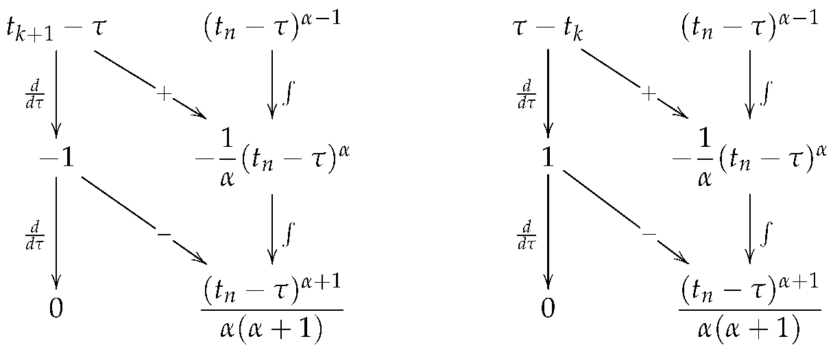 Calculating the corresponding diagonal products between the functions connected by the corresponding arrows and their corresponding signs, one obtains
Substituting the previous results into (16) allows us to obtain
Calculating the corresponding diagonal products between the functions connected by the corresponding arrows and their corresponding signs, one obtainsRemark 2.
The trapezoidal method is obtained by evaluating (19) with , i.e.,
The numerical method in (19) explicitly shows how each segment of the function contributes to the fractional operator’s memory; however, it evaluates the contribution of twice in consecutive loops. To improve computational efficiency, the first step is to expand (19) as follows:
where
and
By grouping the sums and simplifying,
so that (19) is rewritten as
Defining
Equation (21) is expressed as the fractional trapezoidal method
Remark 3.
According to [51], the following equation holds for any whole number r:
In the previous analysis, the simplification of follows from (25).
Remark 4.
The coefficients belonging to the same value of are grouped together in Method (24), reducing the round-off error and the inaccuracies we get by taking a certain number of decimal places instead of taking the entire number [52]. Since the weight vector in (22) depends only on the difference , when performing the numerical simulation, the vector is pre-calculated, and the calculation at each step reduces to a dot product between the function history vector and the weight vector , resulting in greater computational speed.
3. Fractional-Order Derivatives and the Short-Memory Principle
In this section, we contrast the Riemann integral with the fractional derivative and the short-memory principle, which we use to optimize the numerical methods in the next section. Readers interested in delving deeper into fractional calculus may consult [44,48,53,54].
Definition 4.
Let and . The operator defined by
is called the Riemann–Liouville fractional differential operator of order α, with the n-th derivative of integer order.
Definition 5.
Let and . For , the operator defined by
is called the Caputo fractional differential operator of order α.
For practical purposes, consider , so that Operator (27) reduces to
As we can see from Operators (26) and (27), the calculation of each derivative at time t involves all the information from the initial time . From a computational point of view, we see later that this has significant repercussions due to resource constraints, such as memory. That is why we must look for ways to reduce the computational cost. One way to address this situation is through the well-known short-memory principle, which relates the approximation error to the memory length L.
- (i)
- Riemann–Liouville derivative of order . Let be the error between and in ; then,If , thenFinally, considering , it follows that , which implies , i.e., . Therefore, the following bound is obtained:
Remark 5.
Inequality (29) can be used to determine memory length L providing the required precision . Then, to ensure (the estimation error), the memory length should satisfy
in order to satisfy the short-memory principle
- (ii)
- Caputo derivative of order . In a similar manner to the previous case, the error is given byFrom Equation (32), defineThen, one hasConsidering the bound and the triangle inequality, it is possible to concludeWhen holds, the memory length must satisfyto fulfill the short-memory principle
Remark 6
([48]). The above result was expected since, for absolutely continuous functions and , the following relation holds:
Figure 4 illustrates the general idea behind the short-memory principle: the classical derivative (of order n) is a local operator because it depends only on the function’s behavior at the evaluation point . In contrast, the fractional derivative is a non-local operator, since the value of the derivative at the point depends on the entire history of the function from an initial point a. Equation (34) states that, when is large, the contribution of the values of near the lower limit a becomes negligible in the calculation of the derivative at , that is, we can define a memory window L to approximate the fractional derivative by considering only the recent interval. This reduces the computational load, since computing an integral over the entire history of a system (a to t) requires memory and processing time that grow indefinitely as increases. By limiting the calculation to a window L, the computational cost becomes constant and manageable [55,56].
Figure 4.
Visualization of the short-memory principle.
4. Numerical Solution of Fractional Differential Equations
A fractional differential equation (FDE) can be defined similarly to ordinary or partial differential equations, i.e., equations that involve fractional-order derivatives of a dependent variable with respect to another independent variable, such as time. Assuming the existence and uniqueness of solutions, this section presents numerical methods based on successive approximations to solve FDE. The idea of successive approximations is simple [57,58,59]; recall that the function is a solution to the initial value problem , if and only if it is a solution to Volterra’s integral equation
Let us now see how to formulate the integral equation problem and the solution method for FDEs.
4.1. Fractional Differential Equations with Caputo Derivative
Let be the fractional-order; the function is a solution of
if and only if it is a solution of Volterra’s integral equation
whose solution can be constructed using the method of successive approximations [44,48]. Evidently, if , we recover the classical initial value problem and its integral—Equation (36). In particular, for , Volterra’s integral in Equation (38) takes the following form:
In contrast to the general exposition of FDE from an analytical point of view, using different valuable methods to determine explicit forms associated with the solution sought in various problems, multiple studies have been carried out to analyze numerical methods to solve FDEs, including error analysis and computational implementation [60,61,62,63,64]. Evaluating Volterra’s integral in Equation (38) at time with initial time ,
Based on the left-fractional rectangular method in (11), it follows Approximation (40) can be determined as
Reducing terms, we have, for ,
Similarly, now using the right-fractional rectangular method in (13), the solution can be approximated for as
Finally, based on the fractional trapezoidal formula in (24), it is straightforward to verify for
In particular, if , Algorithms (41), (42) and (43) take the form of product integration (PI) rules to solve FDEs [61,65]:
- Explicit PI rectangular rule (fractional forward Euler method):
- Implicit PI rectangular rule (fractional backward Euler method):
- Implicit-type trapezoidal rule:
Remark 7.
We obtain classical numerical methods from Algorithms (44) and (45) if . In both cases, the coefficient , which implies
and
Methods (47) and (48) represent the classical forward Euler and backward Euler methods, respectively [49,66]. On the other hand, considering in (46), one has and , so that
Applying Property (25) to the last term of the above equation, it follows that
By grouping the two previous sums, we arrive at the trapezoidal method for solving ordinary differential equations [49,66]:
The calculation of in (45) and (46) depends on itself. However, the solution can be estimated in two phases: the predictor step with Equation (44), which provides an initial estimate of the solution, and later the corrector step with (46), which refines the initial estimate. These ideas allow us to obtain the predictor–corrector (PC) scheme (see [67] for an in-depth discussion regarding the error analysis of this numerical method):
4.2. Fractional Differential Equations with Riemann–Liouville Derivative
Consider the Riemann–Liouville operator in (26) with , and the nonlinear model
where represents the limit at almost all the points of the right-hand side neighborhood of a, i.e., in the set , :
According to [44,48], is a solution of (51) if and only if it is a solution of the Volterra equation
Evaluating Equation (53) at with , we obtain
Now, considering numerical Method (11) with , it follows that
For systems of order , the corresponding integral in Equation (53) is reduced to
with
Taking and , the Explicit PI-RL rectangular rule is given as
5. Practical Aspects for FPGA Implementation of Numerical Methods
The numerical methods presented in the previous section are based on simple operations, which allow us to determine closed forms for computing the n-th iteration of the solution of an FDE. However, each iteration depends on a finite sum that must be computed at each instant, which imposes a considerable computational burden. In this section, we make a small modification to the algorithms to obtain equivalent forms with greater computational advantage, which we use to implement dynamic systems in embedded systems [68].
5.1. Modified Explicit PI Algorithm
According to (44), it is straightforward to obtain the sample n
From (59), the initial condition is expressed as , so that Equation (44) can be written as
Then, after some elementary simplifications, an iterative method for is obtained, i.e.,
It is essential to mention that the iteration for is obtained directly from Algorithm (44) to complete the calculations. Considering that the sum must be performed from to at each iteration of Algorithm (60), we employ the short-memory principle in (34) to reduce the computational cost and physical limitations of embedded systems. Then, for , the iterations of (60) are recalculated as
Defining as a new variable yields . Then, (60) and (61) are rewritten as
and
respectively. Finally, by setting the initial value , use Algorithm (44) for , so that the modified explicit PI algorithm for FPGA implementations has the recursive equation
with
Remark 8.
In particular, for , one has , so we get the classical Euler’s numerical method
5.2. Modified Explicit PC Algorithm
In a similar manner to the previous case, from (46), we get and solve for the value of given by
Substituting the above equation into (50) yields
Combining with the explicit rule in (60) and performing the corresponding simplifications, for , we obtain the following numerical method:
where
and
Remark 9.
If , we obtain and . Numerical Method (67) is reduced to the classical predictor–corrector method
According to the short-memory principle, one has
where . To further simplify the algorithms and obtain a more computationally efficient implementation, let us again consider the change of variables , which implies . Then, Algorithms (67) and (71) are rewritten as
and
respectively.
Finally, we can establish a recursive equation for the modified explicit PC algorithm by setting the initial value , and using Algorithms (44), (62) for and , respectively, that is,
with
Remark 10.
Consider the function in (68) for . By direct substitution, one gets . If , then for all . The most significant value always occurs in iteration , i.e., for all . In addition, the minimum possible value always occurs when (see Appendix B for details). Then, for practical purposes, from algorithm (74), let
for from a determined . Then, considering , one has that
for , and as . This simplification reduces resource use, such as embedded system memory.
Remark 11.
Numerical Methods (64) and (74) consider the short-memory principle. However, because they are expressed as difference equations, L is expressed in terms of the number of samples. With a window memory time and step size h, we have . The pseudocode provided by Algorithms A1 and A2 describes each numerical method.
6. Numerical and Experimental Results
Fractional-order derivatives introduce a memory effect that captures long-range temporal dependencies, enabling the more accurate modeling of real-world phenomena than integer-order approaches [69]. In chaotic systems, this intrinsic memory enhances dynamical complexity, ergodicity, and the emergence of hidden attractors, making fractional-order models particularly attractive for a wide range of applications.
Despite these advantages, the numerical solution of fractional-order differential equations is considerably more demanding than in the integer-order case. Each state depends on the entire history of previous states, leading to high computational and memory requirements. Numerical methods based on definitions such as Caputo, Grünwald–Letnikov (GL), or Riemann–Liouville (RL) involve convolution-like operations that are inefficient for real-time execution on general-purpose processors or microcontrollers [70].
To alleviate this burden, the short-memory principle is often employed, which assumes that the influence of distant past states becomes negligible beyond a finite time window. By truncating the memory length, the computational and storage requirements can be significantly reduced, at the cost of a controlled approximation error [25,26]. This trade-off is especially relevant in practical implementations where bounded resources are a constraint.
In this section, we validate the numerical algorithms from the previous section to characterize a family of chaotic systems. We also present numerical results for each family member, along with experimental implementation results on FPGA boards and a PRNG application.
6.1. Generalized Lorenz Family
The generalized Lorenz family consists of a 3-dimensional dynamical system given by
The explicit form of (77) is
where , , , , , , , , , , and are parameters, and their choice allows us to obtain a different chaotic system. Table 1 lists the parameter sets that define the dynamical system family in (78) for .
Table 1.
Parameters of the generalized Lorenz family in (78) considering .
The analysis of Family (78) was presented in [77] using the Grünwald–Letnikov (GL) derivative approach. However, the GL and Caputo derivatives have different properties; therefore, applying parameters from [77] or those associated with integer order does not guarantee that Family (78) will exhibit chaotic behavior. To characterize Family (78) with the Caputo operator, consider two key aspects:
- (1)
- A system with n state variables possesses n Lyapunov exponents , each corresponding to a direction in state space. The largest Lyapunov exponent (LLE) quantifies the rate at which two initially close trajectories diverge or converge. If , nearby trajectories converge, and the system tends toward an equilibrium or stable state. If , trajectories neither converge nor diverge, as in a limit cycle. If , nearby trajectories diverge while remaining bounded, as in a chaotic attractor.
- (2)
- A bifurcation represents a qualitative change in system behavior when a parameter surpasses a critical value. The bifurcation diagram illustrates the transition to chaos and reveals the structure of the parameter region. A single curve in the diagram indicates that the system settles into an equilibrium or a stable fixed point. A curve that successively splits into two, four, and eight branches demonstrates period-doubling behavior. A dense cloud of points indicates chaotic behavior, where the trajectory never repeats.
The bifurcation diagram depicts the long-term states as a parameter varies, while the LLE quantifies the degree of chaos in those states. These metrics are typically plotted against the same parameter and compared. A dense cloud in the diagram corresponds to a positive LLE, whereas a single curve or periodic window corresponds to a negative or zero LLE. The consistency between these indicators strengthens the validity of numerical results, while discrepancies often indicate insufficient simulation time, unremoved transients, or numerical problems.
According to [78,79], Algorithms A1 and A2 calculate the LLE for each system in family (78). Figure 5 and Figure 6 (Algorithm A1) and Figure 7 and Figure 8 (Algorithm A2) show how the fractional order and the short-memory window affect the LLE in each system. In the two-dimensional map of the LLE over and , a black contour marks the level , the border between regular dynamics () and chaotic regime (). For clarity, the LLE surface shows a gray plane at , indicating where the surface crosses from negative to positive values. In contrast to the LLE calculation, we show a 3D point cloud of the state variable against and , with bifurcation diagrams stacked along the memory-window axis. Each horizontal slice is the bifurcation diagram for one .
Figure 5.
Based on Algorithm A1, we quantitatively analyzed the Largest Lyapunov Exponent (LLE), comparing the effects of fractional order and the memory window to assess the short-memory principle. The results correspond to Lorenz system (a–c), the Chen system (d–f), the Burke–Shaw system (g–i), and the Liu system (j–l), respectively.
Figure 6.
Based on Algorithm A1, we quantitatively analyzed the Largest Lyapunov Exponent (LLE), comparing the effects of fractional order and the memory window to assess the short-memory principle. The results correspond to Shimizu–Morioka system (a–c), the Lü system (d–f), and the Yang system (g–i), respectively.
Figure 7.
Based on Algorithm A2, we quantitatively analyzed the Largest Lyapunov Exponent (LLE), comparing the effects of fractional order and the memory window to assess the short-memory principle. The results correspond to Lorenz system (a–c), the Chen system (d–f), the Burke–Shaw system (g–i), and the Liu system (j–l), respectively.
Figure 8.
Based on Algorithm A2, we quantitatively analyzed the Largest Lyapunov Exponent (LLE), comparing the effects of fractional order and the memory window to assess the short-memory principle. The results correspond to Shimizu–Morioka system (a–c), the Lü system (d–f), and the Yang system (g–i), respectively.
In all systems, the sign of the LLE changes at a critical that depends only weakly on once the window is long enough. For the Lorenz system, the transition under Algorithm A1 is near (Figure 5a–c). Chaotic behavior ( up to ≈0.9) appears above it. Chen and Liu have thresholds near (Figure 5d–f,j–l). The Chen system shows a second contour at . The Liu system has a second boundary near with an irregular contour. This points to alternating regular/chaotic windows rather than a single transition. Burke–Shaw has one near 0.89–0.90 (Figure 5g–i). Lü and Yang systems (Figure 6d–i) have several vertical contours and bands at showing multiple transitions between regular and chaotic behavior. In the Shimizu–Morioka system (Figure 6a–c), the transition is more gradual, and the LLE is small (LLE ), with a much longer window time than in the other systems (, ). The contour shows a sink in the point cloud around the transition. The results associated with Algorithm A2 (Figure 7 and Figure 8) shift to higher : for the Lorenz system, the transition is near ; for Chen, it shifts to ; for Burke–Shaw, ; and, for Liu, the first boundary is near .
For small , the contour oscillates strongly in . The oscillations appear as ripples in the 3D surfaces and as striped patterns in the negative-LLE region. Once exceeds approximately s, the contour becomes almost vertical, and the LLE stabilizes. This indicates that a truncated memory window is enough to reproduce the dynamics, which is the central point of the short-memory principle.
The chaotic region appears as two separate blocks of points in . A gap separates them and corresponds to the attractor’s two symmetric wings. The cloud preserves its shape as increases, so the bifurcation structure does not depend on the window length for sufficiently large . Checking that the LLE map and the bifurcation diagram agree, and that both are stable for large , provides evidence that the short-memory scheme is reliable.
To determine the Lyapunov exponents and bifurcation diagrams described above, we used the parameters from Table 2 in conjunction with Algorithms A1 and A2. For all systems, we used an initial condition and a simulation time of s to analyze the effect of s. The only exception is the Shimizu–Morioka system; due to its slow dynamics, we used a simulation time of s, with s for Algorithms A1 and A2.
Table 2.
Specific parameters of System (78) with .
The preceding analysis allows for the characterization of Family (78) modeled by Caputo Derivative (27). Each system uses the parameters in Table 2, with ( for the Shimizu–Morioka system), a simulation time of s ( s for the Shimizu–Morioka system), the memory window s ( s for the Shimizu–Morioka system), and the fractional dynamics governed by . All systems share the same initial condition, . Using Algorithm A1, we obtained the results shown in Figure 9 and Figure 10, which depict the phase-plane projections (–, –, –) and the corresponding chaotic attractor. For Algorithm A2, we used a shorter simulation time for Chen, Burke–Shaw, and Liu ( s); for Lorenz, Lü, and Yang, we used s. For the Shimizu–Morioka system, we used the same parameters as in Algorithm A1. In both cases, . Figure 11 and Figure 12 show the simulation results obtained with Algorithm A2.
Figure 9.
Simulation results considering Algorithm A1 applied to Family (78), showing the phase plane projections and the chaotic attractor of Lorenz system (a,b), the Chen system (c,d), the Burke–Shaw system (e,f), and the Liu system (g,h).
Figure 10.
Simulation results considering Algorithm A1 applied to Family (78), showing the phase plane projections and the chaotic attractor of Shimizu–Morioka system (a,b), the Lü system (c,d), and the Yang system (e,f).
Figure 11.
Simulation results considering Algorithm A2 applied to Family (78), showing the phase plane projections and the chaotic attractor of Lorenz system (a,b), the Chen system (c,d), the Burke–Shaw system (e,f), and the Liu system (g,h).
Figure 12.
Simulation results considering Algorithm A2 applied to Family (78), showing the phase plane projections and the chaotic attractor of Shimizu–Morioka system (a,b), the Lü system (c,d), and the Yang system (e,f).
6.2. FPGA Experiments
Field-Programmable Gate Arrays (FPGAs) offer an effective alternative because their inherent parallelism and reconfigurability suit accelerating the repetitive operations and memory accesses associated with fractional operators. Before implementing a system on an FPGA, you must analyze how its variables and parameters are represented numerically. Floating-point is the usual alternative to fixed-point, but it generally costs more in area, power consumption, and design complexity. Fixed-point arithmetic stores real numbers as scaled integers, so it maps directly onto adders and multipliers, whereas floating-point arithmetic needs operations such as exponent alignment and normalization, which add latency and hardware [80]. Comparative studies report 20–30% gains and considerable logic savings when replacing floating-point with an optimized fixed-point representation [81], and FPGA implementations of fractional-order systems based on product integration commonly adopt fixed-point formats for this reason. The cost is that the word length and scaling must be chosen carefully to avoid overflow and maintain sufficient precision, which precision-tuning and error-analysis techniques can address systematically [82,83].
To experimentally validate the proposed algorithms, the rectangular (REC) and predictor–corrector (PC) methods, based on the Caputo derivative, are implemented on FPGAs and applied to the Lorenz family models in (78), with the parameters indicated in the previous subsection, except for the integration steps. In the implementation, h = 0.004 (0.04 for Shimizu–Morioka) is used for the rectangular method, and h = 0.01 (0.1 for Shimizu–Morioka) for the predictor–corrector method. This is because the predictor–corrector method allows the use of larger integration steps without losing the stability of the algorithm or the chaotic properties of the dynamic models. Both implementations use Q1.11.20, a 32-bit signed fixed-point format with 1 sign bit, 11 integer bits and 20 fractional bits. The integer part holds the state variables and the stored vector-field evaluations without overflow in all fourteen system–method combinations evaluated. The fractional part gives a spacing of between representable values. The vector-field evaluations are the right-hand sides (RHSs) of the system equations, and they are stored for the memory calculations.
Since finite precision can change the dynamics of digitally implemented chaotic systems [84,85], the fractional part is assessed quantitatively. All seven systems are simulated with both methods, using and a memory duration s, except for Shimizu–Morioka, where s. Representations Q1.11.F, with total word length from 16 to 64 bits, are compared against double-precision implementations of the same finite-memory algorithms. Every comparison uses the same nominal initial conditions, parameters, timestep and memory window. The fixed-point simulations reproduce the hardware truncation and the widened intermediate arithmetic, including the quantization of initial values and stored constants.
Short-time trajectory agreement, shown in Figure 13a, is measured with the normalized root-mean-square error (NRMSE)
where and are the state vectors from the fixed-point and double-precision simulations at the same sampling instant, and represents the final sample index. The metric expresses the RMS distance between the trajectories as a percentage of the reference trajectory’s RMS magnitude.
Figure 13.
Accuracy versus fractional precision for Q1.11.F. (a) Maximum short-time NRMSE across seven systems for each method. (b) Aggregate relative error of each complete ROM bank. Errors are percentages on logarithmic axes; points denote evaluated formats and connecting lines guide the eye. Bands mark Q1.11.20 (32 bits); annotations give its largest errors across methods in (a) and coefficient banks in (b).
The comparison covered the first s ( s for the Shimizu–Morioka system), corresponding to 250 REC steps or 100 PC steps. This metric measures short-time agreement, including initial-state quantization and subsequent arithmetic errors. Chaotic sensitivity can amplify these perturbations and produce fluctuating trajectory differences; therefore, we did not interpret the metric as a measure of long-time attractor preservation. Figure 13a shows decreasing errors across the evaluated precisions: the maximum NRMSE among the fourteen cases decreased from at Q1.11.12 to at Q1.11.20. Within the Q1.11.20 comparison windows, the largest instantaneous state-vector difference, normalized by the reference RMS state-vector magnitude, was .
Memory-coefficient accuracy, shown in Figure 13b, was evaluated using the aggregate relative error:
where and are the original and quantized history coefficients. These coefficients weight the contributions of past vector-field evaluations. The metric measures the total absolute coefficient discrepancy relative to the total original coefficient magnitude; it is an aggregate bank error, not the largest error of an individual coefficient. Since the hardware supports any memory length , the analysis covers the complete ROM coefficient tables instead of only the coefficients used for a particular M. Each bank stores the coefficients for lags 1–999 and one zero padding entry, which is left out of the evaluation by restricting the lags to . REC and PC share the predictor-history coefficients, and PC also stores the interior and boundary corrector coefficients. The PC interior coefficient at lag 999 is stored but never used; it is still counted in the physical-ROM analysis because it occupies memory. At each precision, the coefficients are regenerated and rounded to the nearest representable value.
The largest aggregate error among the three banks is shown in Figure 13b to decrease from at Q1.11.12 to at Q1.11.20. At Q1.11.12, 796 predictor, 607 PC interior and 799 PC boundary coefficients were rounded to zero, out of 999 entries per bank. An accessed coefficient that is rounded to zero contributes nothing to the corresponding memory calculation. No nonzero coefficients were rounded to zero at Q1.11.20. This analysis covers the full supported coefficient range, whereas the trajectory accuracy and overflow results apply only to the operating memory windows specified above.
Finite-time surrogate largest Lyapunov exponent (LLE) estimates were used as supplementary dynamical diagnostics (Figure 14, with REC in panel (a) and PC in panel (b)). A tangent vector, representing an infinitesimal state perturbation, was propagated through the finite-memory recurrence using the smooth vector-field Jacobian along the simulated trajectory. After discarding the transient and a memory-window warm-up, the estimate was calculated as
where is the tangent vector before renormalization, is its prescribed norm afterward, R is the number of retained renormalization intervals, and is their total duration. Both the tangent vector and its retained RHS history were rescaled at each renormalization. The accumulated logarithmic growth measures the average perturbation expansion rate in the smooth surrogate model.
Figure 14.
Finite-time smooth-surrogate LLE estimates for the seven systems: (a) REC and (b) PC, with identical vertical scales. Markers show evaluated fixed-point formats, connecting lines guide the eye, and dashed horizontal lines show double-precision references. Hollow black squares flag constant post-transient trajectories. Bands mark Q1.11.20 (32 bits). Positive surrogate estimates alone do not establish chaotic stored trajectories.
At Q1.11.20, all fourteen estimates were positive, with maximum absolute differences from double precision of s−1 for REC and s−1 for PC. Unlike the errors in Figure 13, the estimates in Figure 14 do not vary monotonically with fractional precision, and, since they omit rounding discontinuities and are not classical LLEs of the quantized map, they are taken only as supplementary information about dynamical sensitivity. Positive estimates were even obtained for some constant Shimizu–Morioka trajectories at low precision, so positivity alone does not establish chaotic behavior of the stored trajectories. Overall, Q1.11.20 is supported as a practical common 32-bit representation for the evaluated operating conditions: overflow was avoided by its integer range, and close short-time trajectory agreement and low coefficient errors were obtained with its fractional precision, without any nonzero ROM coefficient being rounded to zero. Wider formats reduced the errors further, but at the cost of longer words.
The RTL architecture shown in Figure 15 implements the fractional-order Lorenz-family systems with Caputo’s incremental rectangular algorithm (Equation (64)). Its arithmetic datapath evaluates the functions , and . A configuration block selects the model parameters listed in Table 2 and the precomputed integration factor , while a global input sets the length M of the short-memory window. The fractional order is fixed at and the time step is s, except for the Shimizu–Morioka system, where s.
Figure 15.
Simplified RTL architecture of the rectangular Caputo algorithm.
The short-memory module, shown in Figure 16, stores the previous function evaluations in a banked circular RAM. Like the rest of the datapath, it works in Q1.11.20, and intermediate products and sums keep extra bits that are rescaled and truncated only when they are stored. The depth of the memory is set directly by the number of samples M. If the memory is specified as a nominal duration , M is obtained outside the hardware from the integration step h:
Figure 16.
Short-memory module of the rectangular architecture.
The hardware does not perform this conversion. The selected value of M is maintained during operation, and changing M or the system requires a reset. At iteration n, the history contains previous evaluations, while the current function evaluation is processed separately. The implementation supports and uses 10 RAM banks of 100 words, each 96 bits wide to store the three 32-bit function evaluations. Circular addressing updates the history without shifting stored samples.
To accommodate the limited DSP resources of the DE1-SoC FPGA, a multiply–accumulate architecture evaluates the short-memory sums. Ten multiplier lanes process the history in batches of up to ten terms. A coefficient ROM supplies the weights, while bank-selection logic aligns the corresponding samples and coefficients. The same lanes are reused across batches and sequentially for the three functions, keeping the multiplier count independent of M. A reduction tree combines the ten products, and the resulting sums are accumulated in three registers. The final batch sets unused lanes to zero.
A local controller manages memory access and accumulation. The main finite-state machine (FSM) starts the short-memory calculation and updates the state register only after the historical sums are ready. At the same update edge, the held current function evaluations are written into RAM for the next numerical step. The history-validity counter is cleared during reset so that uninitialized RAM contents are ignored.
The synthesized memory capacity is determined by , whereas the computation time depends on the selected M. Thus, changing changes the number of processed history terms without changing the allocated RAM, ROM, or multiplier resources. For 32-bit samples and coefficients, with a multiple of 10, the nominal storage is
giving a total of bits. The coefficient ROM contains rows of 320 bits, including one unused coefficient position.
With a fully populated memory window and , each step uses previous evaluations per function. For the pipelined controller, the interval between successive state updates is
The five cycles per batch account for memory access, batch loading, and the processing of the three function sums; the additional cycles cover the pipelined function evaluation, controller sequencing, and state update. During initialization, the shorter available history reduces the required number of batches. At clock frequency , the computation time per numerical step is
The architecture was described in VHDL and synthesized using Intel Quartus Prime. The resulting RTL schematic, shown in Figure 17, illustrates the shared equation evaluator, parameter-selection logic, short-memory module, controller, and state registers.
Figure 17.
Quartus-generated RTL schematic of the rectangular architecture.
On the other hand, the predictor–corrector (PC) topology described in Equation (74) extends the rectangular architecture. First, the circuit computes the predicted state and subsequently the corrected state . The same pipelined equation evaluator is reused to calculate the nonlinear functions at the current and predicted states.
Figure 18 shows the PC architecture, and Figure 19 details the short-memory module. The history RAM retains the same 10-bank organization as REC. A shared ten-lane multiply–accumulate unit sequentially calculates the three predictor and three corrector history sums, using their respective coefficient sets. For the corrector, the coefficient associated with the oldest retained evaluation is selected separately, as required by the short-memory formulation. The same integration-factor multipliers are also reused in the predictor and corrector updates.
Figure 18.
Simplified RTL architecture of the Caputo predictor–corrector algorithm.
Figure 19.
Short-memory module of the predictor–corrector architecture.
A Moore FSM coordinates the evaluation of the current functions, short-memory sums, prediction, evaluation at the predicted state, and correction. The corrected state and the current function evaluations are then stored for the next step. The additional predictor registers and arithmetic increase hardware utilization, but no second ten-multiplier short-memory unit is required.
The PC coefficient ROM stores three 32-bit coefficients per history position, organized as rows of 960 bits. The nominal RAM storage remains bits, while the ROM requires bits, giving bits in total. With a full memory window and , the pipelined PC controller requires
clock cycles per state update. Each batch includes two memory-access/loading cycles and six cycles for the predictor and corrector history sums. The additional cycles correspond to equation evaluations and the prediction/correction updates. The Quartus-generated RTL schematic of the PC architecture is shown in Figure 20.
Figure 20.
Quartus-generated RTL schematic of the predictor–corrector architecture.
Regarding resource consumption, Table 3 summarizes the Quartus Prime post-fit results for both architectures on the Cyclone V 5CSEMA5F31C6 FPGA. For a common nominal short-memory duration of s ( s for the Shimizu–Morioka system), Equation (82) gives for REC and for PC. Once these windows are filled, Equations (84) and (86) give 261 and 175 clock cycles per state update, respectively.
Table 3.
Post-fit FPGA resource utilization, estimated state-generation rates for fully populated short-memory windows, and estimated thermal power for Lorenz at 50 MHz. Percentages refer to available Cyclone V resources.
The state-generation rates are theoretical estimates calculated as
using the worst-case post-fit and full-window latency. Each generated state vector contains the simultaneous values ; these rates describe the computational architectures rather than the external visualization hardware. Although PC requires more DSP and memory resources and has a lower , its larger selected integration step reduces the number of history terms required for the same nominal memory duration, yielding a higher estimated state-generation rate under the reported configurations.
The short-memory module uses 30 DSP blocks in each architecture, while the common function evaluator uses 24. The state-update datapath requires 6 DSP blocks for REC and 15 for PC. The logical memory requirements correspond to 38 and 54 physical M10K blocks, respectively, after Quartus mapping.
Power was estimated using the Quartus Power Analyzer with activity from functional simulation supplemented by vectorless estimation. These estimates correspond to a common 50 MHz clock, typical device characteristics, and a 25 °C ambient temperature; HPS power is excluded, and both estimates are classified as low confidence by Quartus. Under these configurations, PC’s estimated core dynamic power is 10.8% higher than REC’s, while its estimated total thermal power is only 1.1% higher. The smaller relative difference in total power reflects the dominant core static component, approximately 412 mW in both architectures.
Table 4 comparatively provides an overview of the proposed architectures for FPGA implementations of fractional-order dynamic systems reported in the literature. Previous work has explored various numerical and architectural strategies, including integration schemes based on rectangular and trapezoidal approximations, the Grünwald–Letnikov methods, reconfigurable implementations, and frequency-domain approximations. Taken together, these studies demonstrate the feasibility of implementing fractional-order systems in programmable hardware and of adjusting certain numerical or configuration parameters. However, the comparison also shows that implementation characteristics are not always documented consistently, particularly with regard to memory usage, clock cycles per update, maximum frequency, power consumption, and specific selection and reconfiguration mechanisms. In addition, this comparison positions the proposed work within the context of integrating diverse models, configuring short-term memory, and evaluating two numerical schemes using explicit implementation metrics. Unlike previous studies in which some of these indicators are unavailable or cannot be verified, the characterization presented here allows for a joint analysis of resource utilization, maximum frequency, update latency, and estimated power consumption. However, since the studies considered use different devices, arithmetic representations, algorithms, and evaluation conditions, these results do not allow us to conclude that the proposed architectures are universally more efficient. Their main comparative value lies in providing a reproducible characterization of two implementation alternatives and demonstrating how the choice of numerical method affects the trade-off between hardware resources and temporal performance.
Table 4.
Comparative hardware analysis of the proposed FPGA implementations of fractional-order chaotic systems. NR: not reported or not verifiable from the original paper.
Figure 21 shows the experimental setup used to visualize the FPGA-generated chaotic attractors through a 16-bit digital-to-analog converter (DAC) and a digital oscilloscope.
Figure 21.
Experimental setup with the DE1-SoC FPGA, 16–bit DAC, and oscilloscope.
The experimental chaotic time series of each system of the Lorenz family in (78), obtained with the parameters described previously and numerical Method (64), are presented in Figure 22 and Figure 23. The oscilloscope allows the phase plane projections to be obtained, which validate the chaotic attractors previously determined numerically. In contrast, the experimental results associated with numerical Method (74) are shown in Figure 24 and Figure 25.
6.3. PRNG Application
Pseudo-Random Number Generators (PRNGs) are essential components in modern cryptographic systems, where they are used to generate keys, nonces, and masks whose unpredictability directly impacts overall security. Unlike true random number generators (TRNGs), which exploit physical phenomena and are inherently non-reproducible, PRNGs are deterministic algorithms that produce reproducible sequences fully defined by an initial secret seed. This determinism makes them attractive for digital hardware, offering high throughput and easy integration, but also places strict requirements on statistical quality, period length and resistance to cryptanalytic attacks [89,90,91].
Chaotic dynamical systems have emerged as promising building blocks for PRNG design, owing to properties such as ergodicity, topological mixing and extreme sensitivity to initial conditions and parameters. These characteristics can be mapped to desirable cryptographic features like diffusion, confusion and high key sensitivity, and many chaos-based PRNGs have been shown to pass stringent statistical batteries such as NIST SP 800-22, TestU01 and ENT, as well as key-space and correlation analyses [90,92,93,94].
To further enhance randomness and enlarge the key space, several works combine multiple chaotic maps, introduce turbulence or cross-over operations between maps, or add perturbation and scrambling stages before bit extraction [90,92,94,95].
However, when chaotic systems are implemented digitally, the finite precision of arithmetic leads to orbit quantization, short periods, and the possible loss or degradation of chaos, a phenomenon that is particularly relevant for fixed-point realizations preferred in FPGA designs due to their simplicity, low resource usage, and high clock frequencies [91,96]. A variety of countermeasures have been proposed to mitigate this dynamic degradation, including the dynamic perturbation of the state, weak coupling of several maps, conservative systems with controlled repetition rates, and careful selection of fixed-point formats guided by finite-precision period analysis [90,97,98].
Within this context, chaotic PRNGs implemented with sufficient resolution on FPGA can generate long-period sequences that closely approximate their continuous-time behavior, achieving a favorable trade-off between hardware efficiency and statistical quality, and making them promising candidates for high-speed stream ciphers and lightweight security applications [99,100,101,102].
To generate pseudorandom sequences from the digitally implemented fixed-point chaotic system, a simple post-processing method is applied in this work. This approach uses a bitwise XOR operation on the least significant bits (LSBs), which typically exhibit faster variations than the most significant bits (MSBs). In the evaluated configuration, the eight LSBs of the and state variables are combined to obtain one 8-bit pseudorandom number per accepted state update:
where and denote the 32-bit fixed-point representations of and at update n, respectively. For the predictor–corrector topology, extraction is performed from the corrected state. The proposed post-processing scheme is illustrated in Figure 26.
Figure 26.
Method for obtaining 8-bit pseudorandom numbers from 32-bit fixed-point chaotic variables.
The PRNG evaluation considers the Lorenz system for both topologies, with fractional order , parameters , and common initial conditions , quantized to Q1.11.20. The rectangular topology uses s and , whereas the predictor–corrector topology uses s and , corresponding to a common nominal short-memory duration of 2 s.
Since one 8-bit word is extracted per accepted state update, the steady-state bit rate supported by each chaotic core is
where is the clock frequency and is the number of clock cycles between accepted state updates. At 50 MHz, with the configured short-memory windows filled, the rectangular and predictor–corrector cores require 261 and 175 clock cycles per update, respectively. Table 5 summarizes the corresponding update intervals and bit rates. The predictor–corrector configuration supports an approximately higher rate because its larger integration step allows fewer memory samples for the same nominal memory duration, reducing the update interval despite the additional correction stage.
Table 5.
Core-derived generation throughput for 8-bit output words at 50 MHz with filled short-memory windows.
Finally, the statistical quality of the proposed pseudorandom number generators is evaluated using the NIST statistical test suite. After discarding an initial transient corresponding to 30 s of model time, a total of 1 billion bits, equivalent to 125 million 8-bit numbers, is collected directly from the FPGA implementation of each topology. Each dataset is divided into 1000 consecutive sequences of 1 million bits, using the default test parameters of NIST STS 2.1.2 [103].
This suite comprises 15 statistical test families that compare the evaluated sequences against an ideal random binary source, yielding 188 subtest results. Individual sequences pass a subtest when their p-value is greater than or equal to . At the second level, the distribution of p-values is assessed for uniformity using a minimum p-value of , while the passing proportion is evaluated using the integer count thresholds implemented in STS 2.1.2, derived from the three-sigma interval. The Random Excursions and Random Excursions Variant proportions use only the eligible sequences: 594 for rectangular and 631 for predictor–corrector.
Table 6 summarizes the NIST results obtained for both topologies. For test families producing multiple outputs, the minimum uniformity p-value and the minimum passing proportion are reported separately. Both methods satisfy all acceptance checks reported by STS 2.1.2.
Table 6.
Results of NIST statistical tests for rectangular and predictor–corrector topologies using 1 billion bits per method. The reported p-values assess the uniformity of individual sequence p-values. The p-value and proportion minima are computed independently across each family’s subtests.
To complement the NIST evaluation, the same binary streams are tested using the Rabbit, Alphabit and BlockAlphabit binary-file batteries of TestU01 1.2.3 [104]. BlockAlphabit is applied with block sizes 1, 2, 4, 8, 16 and 32. A reported statistic is considered suspicious when its p-value falls outside . Table 7 summarizes the numbers of statistics within this interval; these counts refer to reported statistics, rather than sequence passing proportions.
Table 7.
Results of the TestU01 binary-stream batteries for rectangular and predictor–corrector topologies using 1 billion bits per method.
All three tested TestU01 batteries are successfully passed by both methods, with no suspicious p-values. The reported results support the statistical quality of the proposed generators for the evaluated configurations and stream lengths; statistical testing alone does not establish cryptographic security [103].
7. Conclusions
This work combines the dynamical characterization and FPGA implementation of seven fractional-order Lorenz-family systems using Caputo-based rectangular (REC) and predictor–corrector (PC) schemes with the short-memory principle. LLE maps and bifurcation diagrams obtained by varying both the fractional order and memory duration characterize the dynamical regimes within the investigated parameter ranges and guide the selection of finite-memory operating conditions. The effect of truncation was assessed through the consistency of these maps across , not against a full-memory reference solution.
The precision assessment supports Q1.11.20 as a practical representation for the evaluated configurations. Across the fourteen system–method combinations, fixed-point simulations produced a maximum short-time NRMSE of approximately 0.065% relative to the corresponding double-precision reference. These comparisons precede history truncation and therefore quantify finite-precision effects over the evaluated intervals. The coefficient-error assessment and supplementary smooth-surrogate LLE estimates provide additional information for selecting the arithmetic format.
We implemented separate REC and PC architectures on a Cyclone V FPGA, each supporting selection among the seven models and memory lengths from 1 to 1000 samples. After a reset, model and memory settings can be changed without modifying the HDL code or resynthesizing the design. Within each architecture, the maximum supported memory capacity determines resource allocation, while the selected memory length determines the processing workload and update latency. The hardware comparison quantifies resource utilization, timing, estimated throughput, and estimated power under the reported configurations. REC requires fewer hardware resources, whereas PC achieves a higher estimated state-generation rate because its larger selected timestep requires fewer history samples for the same nominal memory duration. Experimental phase portraits obtained through DAC-based oscilloscope measurements complement the numerical characterization.
The implementations also support a PRNG application that extracts pseudorandom bits from the state variables of the selected Lorenz-family model. We performed statistical evaluation in the Lorenz configuration for both REC and PC. The resulting streams met the acceptance criteria in NIST SP 800-22 and the Rabbit, Alphabit, and BlockAlphabit batteries of TestU01. These findings support the statistical quality of the evaluated streams under the specified conditions. Potential applications in secure communications and IoT require further cryptanalytic assessment.
The Riemann–Liouville formulation remains theoretical, since we must close a gap in the numerical analysis before we can implement and validate it on an FPGA. The proposal for the iterative method, as well as the characterization of the Lorenz family via the Riemann–Liouville derivative, remains an open problem for future study.
Author Contributions
J.A.G.-G.: Data curation, Formal analysis, Investigation, Methodology, Software, Visualization, Writing—original draft, Writing—review and editing; O.M.-F.: Conceptualization, Formal analysis, Funding acquisition, Investigation, Methodology, Project administration, Resources, Supervision, Validation, Writing—original draft, Writing—review and editing; J.M.T.-A.: Data curation, Investigation, Software, Visualization, Writing—original draft; O.G.-F.: Data curation, Formal analysis, Investigation, Software, Visualization, Writing—original draft; E.T.-C.: Project administration, Resources, Supervision, Validation, Writing—review and editing; J.d.J.R.-M.: Project administration, Resources, Supervision, Validation, Writing—review and editing. All authors have read and agreed to the published version of the manuscript.
Funding
This research received no external funding.
Data Availability Statement
The raw data supporting the conclusions of this article will be made available by the authors on request.
Conflicts of Interest
The authors declare no conflicts of interest.
Appendix A. Pseudocode Listings
| Algorithm A1 Incremental explicit left-rectangle product-integration algorithm with the short-memory principle | |
| Require: Initial condition , initial time , step size h, fractional order , requested memory duration , number of iterations N, and system function | |
| 1: | ▹ Memory length in samples |
| 2: | ▹ Realized memory duration |
| 3: | |
| 4: // Precompute the incremental history coefficients | |
| 5: for do | |
| 6: | |
| 7: end for | |
| 8: | |
| 9: | |
| 10: for do | |
| 11: | ▹ Number of retained history terms |
| 12: | ▹ Current contribution |
| 13: // Incorporate the retained fractional memory | |
| 14: for do | |
| 15: | |
| 16: end for | |
| 17: | ▹ State update |
| 18: | |
| 19: | |
| 20: end for | |
| 21: return | |
| Algorithm A2 Incremental predictor–corrector product-integration algorithm with the short-memory principle | |
| Require: Initial condition , initial time , step size h, fractional order , requested memory duration , number of iterations N, and system function | |
| 1: | ▹ Memory length in samples |
| 2: | ▹ Realized memory duration |
| 3: | |
| 4: | |
| 5: | |
| 6: // Precompute predictor coefficients | |
| 7: for do | |
| 8: | |
| 9: end for | |
| 10: // Precompute corrector coefficients | |
| 11: for do | |
| 12: | |
| 13: end for | |
| 14: for do | |
| 15: | ▹ |
| 16: end for | |
| 17: | |
| 18: | |
| 19: for do | |
| 20: | ▹ Predictor depth; corrector depth is for |
| 21: // Predictor step | |
| 22: | |
| 23: for do | |
| 24: | |
| 25: end for | |
| 26: | |
| 27: | |
| 28: if then | |
| 29: | ▹ Use the rectangular rule for the first two steps |
| 30: else | |
| 31: | |
| 32: // Corrector step | |
| 33: | |
| 34: for do | |
| 35: | |
| 36: end for | |
| 37: | ▹ Initial history term |
| 38: | |
| 39: end if | |
| 40: | ▹ Store accepted RHS only |
| 41: end for | |
| 42: return | |
Appendix B. Behavior of the Function
The values that Function (68) takes as iterations are performed in the numerical method decrease until they reach zero, i.e.,
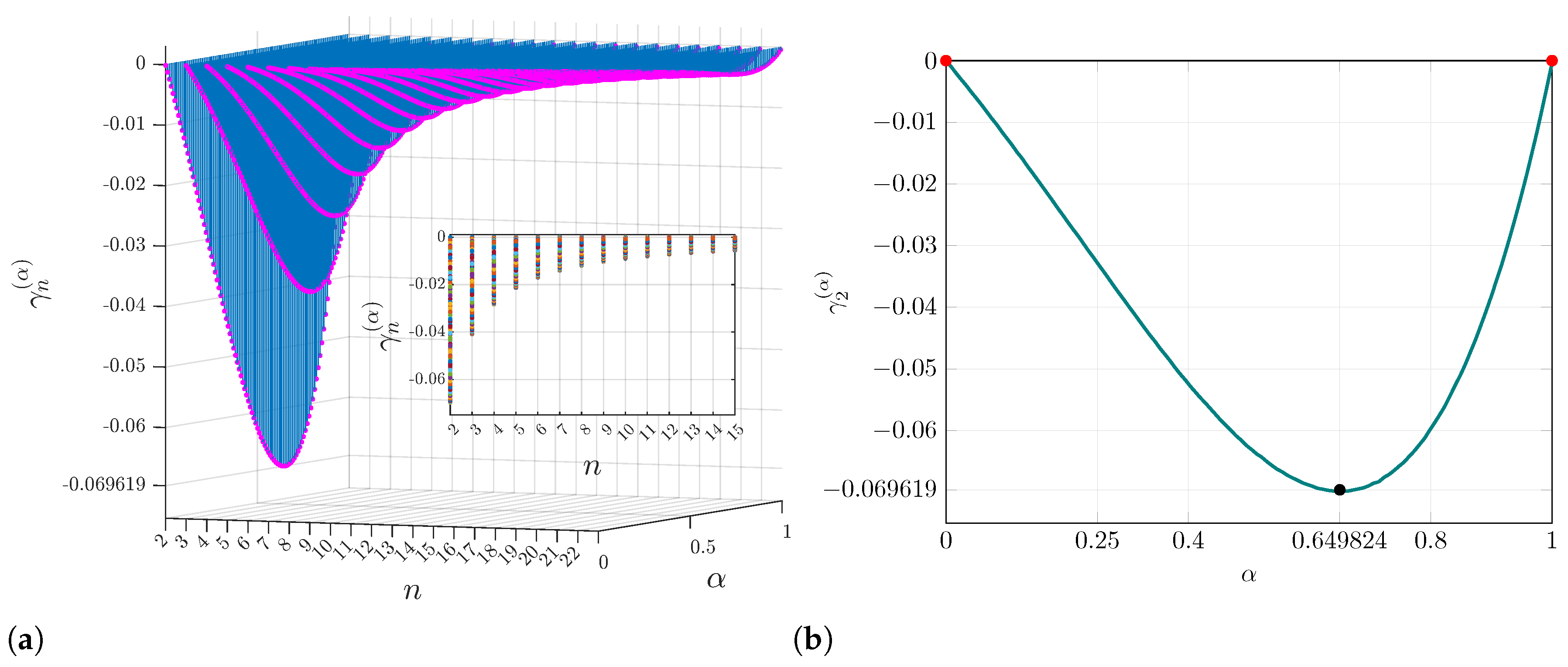
The most interesting part is that the function always takes minimal values (close to zero) starting from iteration , as shown in Figure A1a, and continues to decline asymptotically, fulfilling that . Note that the most significant value always occurs at iteration , i.e., for all . In addition, the maximum possible value always occurs at , as shown in Figure A1b.
Figure A1.
Behavior of Function (68) considering the interval : (a) Function in the interval , (b) Function to show the minimum value.
Appendix C. Modified Explicit PI-RL Algorithm
The main part of this article focuses on the analysis and digital implementation—on an FPGA—of the Lorenz family using the Caputo operator. Regarding the Riemann–Liouville case, we have made some initial progress, but it still requires validation. From Algorithm (58), for , we obtain
and the sample n given as . Considering , it follows that
Substituting (A2) into (58) and simplifying, note that
By reducing the coefficients, we find that we can define the next coefficient as
so that
Finally, according to the short-memory principle, one has
with
Remark A1.
To implement (A4) numerically, consider three interesting situations:
- (i)
- Consider the value of (57) as a finite constant, i.e., . Since , then . As the simulation grid is refined and , the value , representing the singularity at the initialization time [53]. For example, consider the FDE , with initial condition . According to (56), the corresponding integral equation has the formso thatTaking the initial approximation as , thenand so on, so that . Finally, asymptotically, we have that . Note how the solution exhibits a singularity at , i.e., . Finally,which implies
- (ii)
- If is a finite constant, thenIf behaves like a finite constant near , we get
- (iii)
- The trivial situation occurs if , so that .
Analysis of chaotic systems: From the previous analysis, note that, for to be non-zero, the system must necessarily exhibit a singularity at initialization. If we consider chaotic systems initialized with very large values (result of the singularity and a small value h), will further amplify the singularity, causing a numerical overflow in the first iteration, unless h is chosen very carefully to avoid numerical instability. Considering the second case, we must program ; however, this forces the initial state to be the origin for any system lacking this singularity. In most chaotic systems, the origin is an equilibrium point, so the system will be trapped at the origin for all iterations, so the trajectory stays there and never reaches the attractor [77,105,106].
References
- Gorenflo, R.; Mainardi, F. Fractional Calculus: Integral and Differential Equations of Fractional Order. arXiv 2008, arXiv:0805.3823. [Google Scholar]
- David, S.; Linares, J.L.; Pallone, E. Fractional order calculus: Historical apologia, basic concepts and some applications. Rev. Bras. Ensino Fis. 2011, 33, 4302. [Google Scholar] [CrossRef] [Scilit]
- Ortigueira, M.; Machado, J. What is a fractional derivative? J. Comput. Phys. 2015, 293, 4–13. [Google Scholar] [CrossRef] [Scilit]
- Al-Mdallal, Q.; Abdeljawad, T.; Hajji, M. Theoretical and Numerical Results for Fractional Difference and Differential Equations. Discret. Dyn. Nat. Soc. 2017, 2017, 2543452. [Google Scholar] [CrossRef] [Scilit]
- Gutiérrez, R.; Rosário, J.M.; Machado, J. Fractional Order Calculus: Basic Concepts and Engineering Applications. Math. Probl. Eng. 2010, 2010, 375858. [Google Scholar] [CrossRef] [Scilit]
- Suzuki, J.; Gulian, M.A.; Zayernouri, M.; D’Elia, M. Fractional Modeling in Action: A Survey of Nonlocal Models for Subsurface Transport, Turbulent Flows, and Anomalous Materials. J. Peridynamics Nonlocal Model. 2021, 5, 392–459. [Google Scholar] [CrossRef] [Scilit]
- Wu, G.-C.; Deng, Z.-G.; Baleanu, D.; Zeng, D.-Q. New variable-order fractional chaotic systems for fast image encryption. Chaos 2019, 29, 083103. [Google Scholar] [CrossRef] [Scilit] [PubMed]
- Muñoz-Pacheco, J.; Zambrano-Serrano, E.; Volos, C.; Jafari, S.; Kengne, J.; Rajagopal, K. A New Fractional-Order Chaotic System with Different Families of Hidden and Self-Excited Attractors. Entropy 2018, 20, 564. [Google Scholar] [CrossRef] [Scilit] [PubMed]
- Danca, M.F. Hidden chaotic attractors in fractional-order systems. Nonlinear Dyn. 2018, 89, 577–586. [Google Scholar] [CrossRef] [Scilit]
- Rahman, Z.A.S.A.; Jasim, B.H. Hidden Dynamics Investigation, Fast Adaptive Synchronization, and Chaos-Based Secure Communication Scheme of a New 3D Fractional-Order Chaotic System. Inventions 2022, 7, 108. [Google Scholar] [CrossRef] [Scilit]
- Roohi, M.; Zhang, C.; Taheri, M.; Basse-O’Connor, A. Synchronization of Fractional-Order Delayed Neural Networks Using Dynamic-Free Adaptive Sliding Mode Control. Fractal Fract. 2023, 7, 682. [Google Scholar] [CrossRef] [Scilit]
- Aguirre, J.; Viana, R.; Sanjuán, M. Fractal structures in nonlinear dynamics. Rev. Mod. Phys. 2009, 81, 333–386. [Google Scholar] [CrossRef] [Scilit]
- Lin, H.; Deng, X.; Yu, F.; Sun, Y. Diversified Butterfly Attractors of Memristive HNN With Two Memristive Systems and Application in IoMT for Privacy Protection. IEEE Trans. Comput.-Aided Des. Integr. Circuits Syst. 2025, 44, 304–316. [Google Scholar] [CrossRef] [Scilit]
- Cattani, M.; Caldas, I.; Souza, S.D.; Iarosz, K. Deterministic Chaos Theory: Basic Concepts. Rev. Bras. Ensino Fis. 2016, 39, e1309. [Google Scholar] [CrossRef] [Scilit]
- Lorenz, E.N. Deterministic nonperiodic flow. J. Atmos. Sci. 1963, 20, 130–141. [Google Scholar] [CrossRef] [Scilit]
- Gu, Y.; Li, G.; Xu, X.; Song, X.; Wu, S. Multistable dynamics and attractors self-reproducing in a new hyperchaotic complex Lü system. Chaos 2023, 33, 093112. [Google Scholar] [CrossRef] [Scilit] [PubMed]
- Wang, M.; Deng, Y.; Liao, X.; Li, Z.; Ma, M.; Zeng, Y. Dynamics and circuit implementation of a four-wing memristive chaotic system with attractor rotation. Int. J. Non-Linear Mech. 2019, 111, 149–159. [Google Scholar] [CrossRef] [Scilit]
- Kopp, M.; Samuilik, I. A New 6D Two-wing Hyperchaotic System: Dynamical Analysis, Circuit Design, and Synchronization. Chaos Theory Appl. 2024, 6, 273–283. [Google Scholar] [CrossRef] [Scilit]
- Yuan, Y.; Yu, F.; Tan, B.; Huang, Y.; Yao, W.; Cai, S.; Lin, H. A class of n-D Hamiltonian conservative chaotic systems with three-terminal memristor: Modeling, dynamical analysis, and FPGA implementation. Chaos 2025, 35, 013121. [Google Scholar] [CrossRef] [Scilit] [PubMed]
- Grassi, G. Chaos in the Real World: Recent Applications to Communications, Computing, Distributed Sensing, Robotic Motion, Bio-Impedance Modelling and Encryption Systems. Symmetry 2021, 13, 2151. [Google Scholar] [CrossRef] [Scilit]
- Yu, F.; Li, L.; Tang, Q.; Cai, S.; Song, Y.; Xu, Q. A Survey on True Random Number Generators Based on Chaos. Discret. Dyn. Nat. Soc. 2019, 2019, 2545123. [Google Scholar] [CrossRef] [Scilit]
- Aliabadi, F.; Majidi, M.; Khorashadizadeh, S. Chaos synchronization using adaptive quantum neural networks and its application in secure communication and cryptography. Neural Comput. Appl. 2022, 34, 6521–6533. [Google Scholar] [CrossRef] [Scilit]
- Devi, R.P.; Khan, M.I. Comparative Analysis of Fractional Derivative Operators: Stability, Asymptotic Behavior, and Computational Challenges. Int. J. Res. Sci. Technol. 2024, 14, 13–23. [Google Scholar] [CrossRef] [Scilit]
- Yu, X.; Xu, H.; Mao, Z.; Sun, H.; Zhang, Y.; Zhang, D.; Chen, Y. A data-driven framework for discovering fractional differential equations in complex systems. Nonlinear Dyn. 2024, 113, 24557–24577. [Google Scholar] [CrossRef] [Scilit]
- Wei, Y.; Chen, Y.; Cheng, S.; Wang, Y. A note on short memory principle of fractional calculus. Fract. Calc. Appl. Anal. 2017, 20, 1382–1404. [Google Scholar] [CrossRef] [Scilit]
- Deng, W. Short memory principle and a predictor-corrector approach for fractional differential equations. J. Comput. Appl. Math. 2007, 206, 174–188. [Google Scholar] [CrossRef] [Scilit]
- Abdelaty, A.; Roshdy, M.; Said, L.; Radwan, A.G. Numerical Simulations and FPGA Implementations of Fractional-Order Systems Based on Product Integration Rules. IEEE Access 2020, 8, 102093–102105. [Google Scholar] [CrossRef] [Scilit]
- He, S.; Sun, K.; Wang, H. Complexity Analysis and DSP Implementation of the Fractional-Order Lorenz Hyperchaotic System. Entropy 2015, 17, 8299–8311. [Google Scholar] [CrossRef] [Scilit]
- Piper, J.R.; Sprott, J. Simple Autonomous Chaotic Circuits. IEEE Trans. Circuits Syst. II Express Briefs 2010, 57, 730–734. [Google Scholar] [CrossRef] [Scilit]
- Clemente-López, D.; Muñoz-Pacheco, J.; Rangel-Magdaleno, J. A Review of the Digital Implementation of Continuous-Time Fractional-Order Chaotic Systems Using FPGAs and Embedded Hardware. Arch. Comput. Methods Eng. 2022, 30, 951–983. [Google Scholar] [CrossRef] [Scilit]
- Pano-Azucena, A.; Ovilla-Martínez, B.; Tlelo-Cuautle, E.; Muñoz-Pacheco, J.; Fraga, L.G.D.L. FPGA-based implementation of different families of fractional-order chaotic oscillators applying Grünwald–Letnikov method. Commun. Nonlinear Sci. Numer. Simul. 2019, 72, 516–527. [Google Scholar] [CrossRef] [Scilit]
- Tolba, M.; Said, L.; Madian, A.; Radwan, A.G. FPGA Implementation of the Fractional Order Integrator/Differentiator: Two Approaches and Applications. IEEE Trans. Circuits Syst. I Regul. Pap. 2019, 66, 1484–1495. [Google Scholar] [CrossRef]
- Tolba, M.; Abdelaty, A.; Soliman, N.; Said, L.; Madian, A.; Azar, A.; Radwan, A.G. FPGA implementation of two fractional order chaotic systems. AEU-Int. J. Electron. Commun. 2017, 78, 162–172. [Google Scholar] [CrossRef] [Scilit]
- Mohamed, S.M.; Sayed, W.; Said, L.; Radwan, A.G. Reconfigurable FPGA Realization of Fractional-Order Chaotic Systems. IEEE Access 2021, 9, 89376–89389. [Google Scholar] [CrossRef] [Scilit]
- Tolba, M.; Saleh, H.; Mohammad, B.; Al-Qutayri, M.; Elwakil, A.; Radwan, A.G. Enhanced FPGA realization of the fractional-order derivative and application to a variable-order chaotic system. Nonlinear Dyn. 2020, 99, 3143–3154. [Google Scholar] [CrossRef] [Scilit]
- Yu, F.; Zhang, W.; Xiao, X.; Yao, W.; Cai, S.; Zhang, J.; Wang, C.; Li, Y. Dynamic Analysis and Field-Programmable Gate Array Implementation of a 5D Fractional-Order Memristive Hyperchaotic System with Multiple Coexisting Attractors. Fractal Fract. 2024, 8, 271. [Google Scholar] [CrossRef] [Scilit]
- Yu, F.; Xu, S.; Xiao, X.; Yao, W.; Huang, Y.; Cai, S.; Li, Y. Dynamic analysis and FPGA implementation of a 5D multi-wing fractional-order memristive chaotic system with hidden attractors. Integration 2024, 96, 102129. [Google Scholar] [CrossRef] [Scilit]
- Yu, F.; Zhang, S.; Su, D.; Wu, Y.; Gracia, Y.M.; Yin, H. Dynamic Analysis and Implementation of FPGA for a New 4D Fractional-Order Memristive Hopfield Neural Network. Fractal Fract. 2025, 9, 115. [Google Scholar] [CrossRef] [Scilit]
- Clemente-López, D.; Muñoz-Pacheco, J.; Zambrano-Serrano, E.; Beltrán, O.G.F.F.; Rangel-Magdaleno, J. A Piecewise Linear Approach for Implementing Fractional-Order Multi-Scroll Chaotic Systems on ARMs and FPGAs. Fractal Fract. 2024, 8, 389. [Google Scholar] [CrossRef] [Scilit]
- Sayed, W.; Roshdy, M.; Said, L.; Herencsar, N.; Radwan, A.G. CORDIC-Based FPGA Realization of a Spatially Rotating Translational Fractional-Order Multi-Scroll Grid Chaotic System. Fractal Fract. 2022, 6, 432. [Google Scholar] [CrossRef] [Scilit]
- Mohamed, S.M.; Sayed, W.; Madian, A.; Radwan, A.G.; Said, L. An Encryption Application and FPGA Realization of a Fractional Memristive Chaotic System. Electronics 2023, 12, 1219. [Google Scholar] [CrossRef] [Scilit]
- Zourmba, K.; Effa, J.; Fischer, C.; Rodríguez-Muñoz, J.D.; Moreno-Lopez, M.F.; Tlelo-Cuautle, E.; de Dieu Nkapkop, J. Fractional order 1D memristive time-delay chaotic system with application to image encryption and FPGA implementation. Math. Comput. Simul. 2024, 227, 58–84. [Google Scholar] [CrossRef] [Scilit]
- He, S.; Yu, F.; Guo, R.; Zheng, M.; Tang, T.; Jin, J.; Wang, C. Dynamic analysis and FPGA implementation of a fractional-order memristive Hopfield neural network with hidden chaotic dual-wing attractors. Fractal Fract. 2025, 9, 561. [Google Scholar] [CrossRef] [Scilit]
- Samko, S.G.; Kilbas, A.A.; Marichev, O.I. Fractional Integrals and Derivatives; Gordon and Breach Science Publishers: Yverdon-les-Bains, Switzerland, 1993; Volume 1. [Google Scholar]
- Artin, E. The Gamma Function; Courier Dover Publications: Garden City, NY, USA, 2015. [Google Scholar]
- Bell, W.W. Special Functions for Scientists and Engineers; Courier Corporation: San Francisco, CA, USA, 2004. [Google Scholar]
- Lebedev, N.N.; Silverman, R.A.; Livhtenberg, D. Special Functions and Their Applications; Prentice-Hall: Hoboken, NJ, USA, 1965. [Google Scholar]
- Diethelm, K. The Analysis of Fractional Differential Equations: An Application-Oriented Exposition Using Differential Operators of Caputo Type; Springer: Berlin/Heidelberg, Germany, 2010. [Google Scholar]
- Cheney, E.W.; Kincaid, D.R. Numerical Mathematics and Computing, 7th ed.; Cengage Learning: Boston, MA, USA, 2013. [Google Scholar]
- Thomas, G.B.; Weir, M.D.; Hass, J. Thomas’ Calculus: Early Transcendentals, 12th ed.; Pearson: London, UK, 2014. [Google Scholar]
- He, T.X. Methods for the Summation of Series; Chapman and Hall/CRC: Boca Raton, FL, USA, 2022. [Google Scholar]
- Burden, R.L.; Faires, J.D. Numerical Analysis, 9th ed.; Brooks/Cole, Cengage Learning: Boston, MA, USA, 2010. [Google Scholar]
- Podlubny, I. Fractional Differential Equations: An Introduction to Fractional Derivatives, Fractional Differential Equations, to Methods of Their Solution and Some of Their Applications; Elsevier: Amsterdam, The Netherlands, 1998; Volume 198. [Google Scholar]
- Miller, K.S.; Ross, B. An Introduction to the Fractional Calculus and Fractional Differential Equations; Wiley-Interscience: Hoboken, NJ, USA, 1993. [Google Scholar]
- Dimov, I.; Georgieva, R.; Todorov, V. Balancing of systematic and stochastic errors in Monte Carlo algorithms for integral equations. In Proceedings of the International Conference on Numerical Methods and Applications; Springer: Cham, Switzerland, 2014; pp. 44–51. [Google Scholar]
- Gong, C.; Bao, W.; Liu, J. A piecewise memory principle for fractional derivatives. Fract. Calc. Appl. Anal. 2017, 20, 1010–1022. [Google Scholar] [CrossRef] [Scilit]
- Lovitt, W.V. Linear Integral Equations; Dover: Garden City, NY, USA, 1924. [Google Scholar]
- Tricomi, F.G. Integral Equations; Dover: Garden City, NY, USA, 1985. [Google Scholar]
- Rahman, M. Integral Equations and Their Applications; WIT Press: Southampton, UK, 2007. [Google Scholar]
- Garrappa, R. Trapezoidal methods for fractional differential equations: Theoretical and computational aspects. Math. Comput. Simul. 2015, 110, 96–112. [Google Scholar] [CrossRef] [Scilit]
- Garrappa, R. Numerical solution of fractional differential equations: A survey and a software tutorial. Mathematics 2018, 6, 16. [Google Scholar] [CrossRef] [Scilit]
- Li, C.; Zeng, F. Numerical Methods for Fractional Calculus; CRC Press: Boca Raton, FL, USA, 2015. [Google Scholar]
- Tacha, O.I.; Munoz-Pacheco, J.M.; Zambrano-Serrano, E.; Stouboulos, I.N.; Pham, V.T. Determining the chaotic behavior in a fractional-order finance system with negative parameters. Nonlinear Dyn. 2018, 94, 1303–1317. [Google Scholar] [CrossRef] [Scilit]
- Owolabi, K.M.; Atangana, A. Numerical Methods for Fractional Differentiation; Springer: Singapore, 2019; Volume 54. [Google Scholar]
- Garrappa, R.; Popolizio, M. On accurate product integration rules for linear fractional differential equations. J. Comput. Appl. Math. 2011, 235, 1085–1097. [Google Scholar] [CrossRef] [Scilit]
- Hildebrand, F.B. Introduction to Numerical Analysis; Courier Corporation: San Francisco, CA, USA, 1987. [Google Scholar]
- Diethelm, K.; Ford, N.J.; Freed, A.D. Detailed error analysis for a fractional Adams method. Numer. Algorithms 2004, 36, 31–52. [Google Scholar] [CrossRef] [Scilit]
- Tlelo-Cuautle, E.; Pano-Azucena, A.D.; Guillén-Fernández, O.; Silva-Juárez, A. Analog/Digital Implementation of Fractional Order Chaotic Circuits and Applications; Springer: Cham, Switzerland, 2020. [Google Scholar]
- He, S.; Wang, H.; Sun, K. Solutions and memory effect of fractional-order chaotic system: A review. Chin. Phys. B 2021, 31, 060501. [Google Scholar] [CrossRef] [Scilit]
- Matusiak, M. Optimization for Software Implementation of Fractional Calculus Numerical Methods in an Embedded System. Entropy 2020, 22, 566. [Google Scholar] [CrossRef] [Scilit] [PubMed]
- Zhou, T.; Tang, Y.; Chen, G. Chen’s attractor exists. Int. J. Bifurc. Chaos 2004, 14, 3167–3177. [Google Scholar] [CrossRef] [Scilit]
- Shaw, R. Strange attractors, chaotic behavior, and information flow. Z. Naturforschung A 1981, 36, 80–112. [Google Scholar] [CrossRef] [Scilit]
- Liu, C.; Liu, T.; Liu, L.; Liu, K. A new chaotic attractor. Chaos Solitons Fractals 2004, 22, 1031–1038. [Google Scholar] [CrossRef] [Scilit]
- Shimizu, T.; Morioka, N. On the bifurcation of a symmetric limit cycle to an asymmetric one in a simple model. Phys. Lett. A 1980, 76, 201–204. [Google Scholar] [CrossRef] [Scilit]
- Lü, J.; Chen, G. A new chaotic attractor coined. Int. J. Bifurc. Chaos 2002, 12, 659–661. [Google Scholar] [CrossRef] [Scilit]
- Yang, Q.; Chen, G. A chaotic system with one saddle and two stable node-foci. Int. J. Bifurc. Chaos 2008, 18, 1393–1414. [Google Scholar] [CrossRef] [Scilit]
- Petráš, I. The fractional-order Lorenz-type systems: A review. Fract. Calc. Appl. Anal. 2022, 25, 362–377. [Google Scholar] [CrossRef] [Scilit] [PubMed]
- Li, H.; Shen, Y.; Han, Y.; Dong, J.; Li, J. Determining Lyapunov exponents of fractional-order systems: A general method based on memory principle. Chaos Solitons Fractals 2023, 168, 113167. [Google Scholar] [CrossRef] [Scilit]
- Danca, M.F.; Kuznetsov, N. Matlab code for Lyapunov exponents of fractional-order systems. Int. J. Bifurc. Chaos 2018, 28, 1850067. [Google Scholar] [CrossRef] [Scilit]
- Winandy, I.; Dion, A.; Manni, F.; Garoche, P.L.; Khalifa, D.B.; Martel, M. Automated Fixed-Point Precision Optimization for FPGA Synthesis. IEEE Open J. Circuits Syst. 2025, 6, 192–204. [Google Scholar] [CrossRef] [Scilit]
- Amin-Nejad, S.; Basharkhah, K.; Gashteroodkhani, T. Floating Point versus Fixed point Tradeoffs in FPGA Implementations of QR Decomposition Algorithm. Eur. J. Electr. Eng. Comput. Sci. 2019, 3, 1–5. [Google Scholar] [CrossRef] [Scilit]
- Sung, W.; Kum, K.I. Simulation-based word-length optimization method for fixed-point digital signal processing systems. IEEE Trans. Signal Process. 1995, 43, 3087–3090. [Google Scholar] [CrossRef] [Scilit]
- Constantinides, G. Word-length optimization for differentiable nonlinear systems. ACM Trans. Des. Autom. Electron. Syst. 2006, 11, 26–43. [Google Scholar] [CrossRef] [Scilit]
- Wang, Q.; Yu, S.; Li, C.; Lu, J.; Fang, X.; Guyeux, C.; Bahi, J. Theoretical Design and FPGA-Based Implementation of Higher-Dimensional Digital Chaotic Systems. IEEE Trans. Circuits Syst. I Regul. Pap. 2015, 63, 401–412. [Google Scholar] [CrossRef] [Scilit]
- Méndez-Ramírez, R.; Arellano-Delgado, A.; Murillo-Escobar, M.; Cruz-Hernández, C. Degradation Analysis of Chaotic Systems and their Digital Implementation in Embedded Systems. Complexity 2019, 2019, 9863982. [Google Scholar] [CrossRef] [Scilit]
- Sayed, W.; Roshdy, M.; Said, L.; Radwan, A.G. Chaotic Dynamics and FPGA Implementation of a Fractional-Order Chaotic System With Time Delay. IEEE Open J. Circuits Syst. 2020, 1, 255–262. [Google Scholar] [CrossRef] [Scilit]
- Lin, L.; Wang, Q.; Cai, G. FPGA Realization of Two Different Fractional-Order Time-Delay Chaotic System With Predefined Synchronization Time. IEEE Access 2022, 10, 133663–133672. [Google Scholar] [CrossRef] [Scilit]
- Perez, J.C.N.; Prieto, R.U.A.; Afolabi, O.; Pinal, F.J.P.; Valdez, M.A.E. FPGA realization of fractional-order chaotic oscillators using ABM and EFORK methods. Sci. Rep. 2026, 16, 19716. [Google Scholar] [CrossRef] [Scilit] [PubMed]
- Dridi, F.; Assad, S.E.; Youssef, W.H.; Machhout, M.; Samhat, A. Design, FPGA-based Implementation and Performance of a Pseudo Random Number Generator of Chaotic Sequences. Adv. Electr. Comput. Eng. 2021, 21, 41–48. [Google Scholar] [CrossRef] [Scilit]
- Cang, S.; Kang, Z.; Wang, Z. Pseudo-random number generator based on a generalized conservative Sprott-A system. Nonlinear Dyn. 2021, 104, 827–844. [Google Scholar] [CrossRef] [Scilit]
- Gomar, S.; Ahmadi, M. A Digital Pseudo Random Number Generator Based on a Chaotic Dynamic System. In 2019 26th IEEE International Conference on Electronics, Circuits and Systems (ICECS); IEEE: Piscataway, NJ, USA, 2019; pp. 610–613. [Google Scholar]
- Krishnamoorthi, S.; Jayapaul, P.; Dhanaraj, R.K.; Rajasekar, V.; Balusamy, B.; Islam, S.H. Design of pseudo-random number generator from turbulence padded chaotic map. Nonlinear Dyn. 2021, 104, 1627–1643. [Google Scholar] [CrossRef] [Scilit]
- Irfan, M.; Khan, M.A. Cryptographically secure pseudo-random number generation using a Robust Chaotic Tent Map: A novel approach. Cogent Eng. 2025, 12, 2558751. [Google Scholar] [CrossRef] [Scilit]
- Dridi, F.; Assad, S.E.; Youssef, W.E.H.; Machhout, M. Design, Hardware Implementation on FPGA and Performance Analysis of Three Chaos-Based Stream Ciphers. Fractal Fract. 2023, 7, 197. [Google Scholar] [CrossRef] [Scilit]
- Krishnamoorthi, S.; Jayapaul, P.; Rajasekar, V.; Dhanaraj, R.K.; Iwendi, C. A futuristic approach to generate random bit sequence using dynamic perturbed chaotic system. Turk. J. Electr. Eng. Comput. Sci. 2021, 30, 35–49. [Google Scholar] [CrossRef] [Scilit]
- Abderrahim, N.W.; Benmansour, F.Z.; Seddiki, O. FPGA Implementation of a Chaotic Pseudo-random Numbers Generator. SN Comput. Sci. 2023, 4, 410. [Google Scholar] [CrossRef] [Scilit]
- Silva, S.J.S.; Cardoso, M.B.R.; Nardo, L.; Nepomuceno, E.; Hübner, M.; Arias-Garcia, J. A New Chaos-Based PRNG Hardware Architecture Using the HUB Fixed-Point Format. IEEE Trans. Instrum. Meas. 2023, 72, 2001208. [Google Scholar] [CrossRef] [Scilit]
- Wang, C.; Zheng, J.; Qian, Y. Structure-Varying Complex Network Chaotic Model and Its Hardware Implementation. IEEE Trans. Circuits Syst. I Regul. Pap. 2025, 72, 4673–4685. [Google Scholar] [CrossRef] [Scilit]
- Gonzalez, J.A.G.; Rangel-Magdaleno, J.; Muñoz-Pacheco, J. FPGA Implementation of a Multi-PRNG Based on a Multiscroll Chaotic Hopfield Neural Network. IEEE Trans. Ind. Inform. 2025, 21, 3097–3106. [Google Scholar] [CrossRef] [Scilit]
- Garcia-Bosque, M.; Pérez-Resa, A.; Sánchez-Azqueta, C.; Aldea, C.; Celma, S. Chaos-Based Bitwise Dynamical Pseudorandom Number Generator On FPGA. IEEE Trans. Instrum. Meas. 2019, 68, 291–293. [Google Scholar] [CrossRef] [Scilit]
- Gupta, M.; Chauhan, R. Hardware Efficient Pseudo-Random Number Generator Using Chen Chaotic System on FPGA. J. Circuits Syst. Comput. 2021, 31, 2250043. [Google Scholar] [CrossRef] [Scilit]
- Hadjadj, M.A.; Kaibou, R.; Sadoudi, S. Design and Hardware Implementation of a PRNG-CS for Embedded Security Applications. In 2025 IEEE Computer Society Annual Symposium on VLSI (ISVLSI); IEEE: Piscataway, NJ, USA, 2025; Volume 1, pp. 1–4. [Google Scholar]
- Rukhin, A.; Soto, J.; Nechvatal, J.; Smid, M.; Barker, E. A Statistical Test Suite for Random and Pseudorandom Number Generators for Cryptographic Applications; Technical Report SP 800-22 Revision 1a; National Institute of Standards and Technology: Gaithersburg, MD, USA, 2010.
- L’Ecuyer, P.; Simard, R. TestU01: A C Library for Empirical Testing of Random Number Generators. ACM Trans. Math. Softw. 2007, 33, 22. [Google Scholar] [CrossRef] [Scilit]
- Sene, N.; Ndiaye, A. On Class of Fractional-Order Chaotic or Hyperchaotic Systems in the Context of the Caputo Fractional-Order Derivative. J. Math. 2020, 2020, 8815377. [Google Scholar] [CrossRef] [Scilit]
- Heymans, N.; Podlubny, I. Physical interpretation of initial conditions for fractional differential equations with Riemann-Liouville fractional derivatives. Rheol. Acta 2006, 45, 765–771. [Google Scholar] [CrossRef] [Scilit]


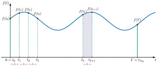
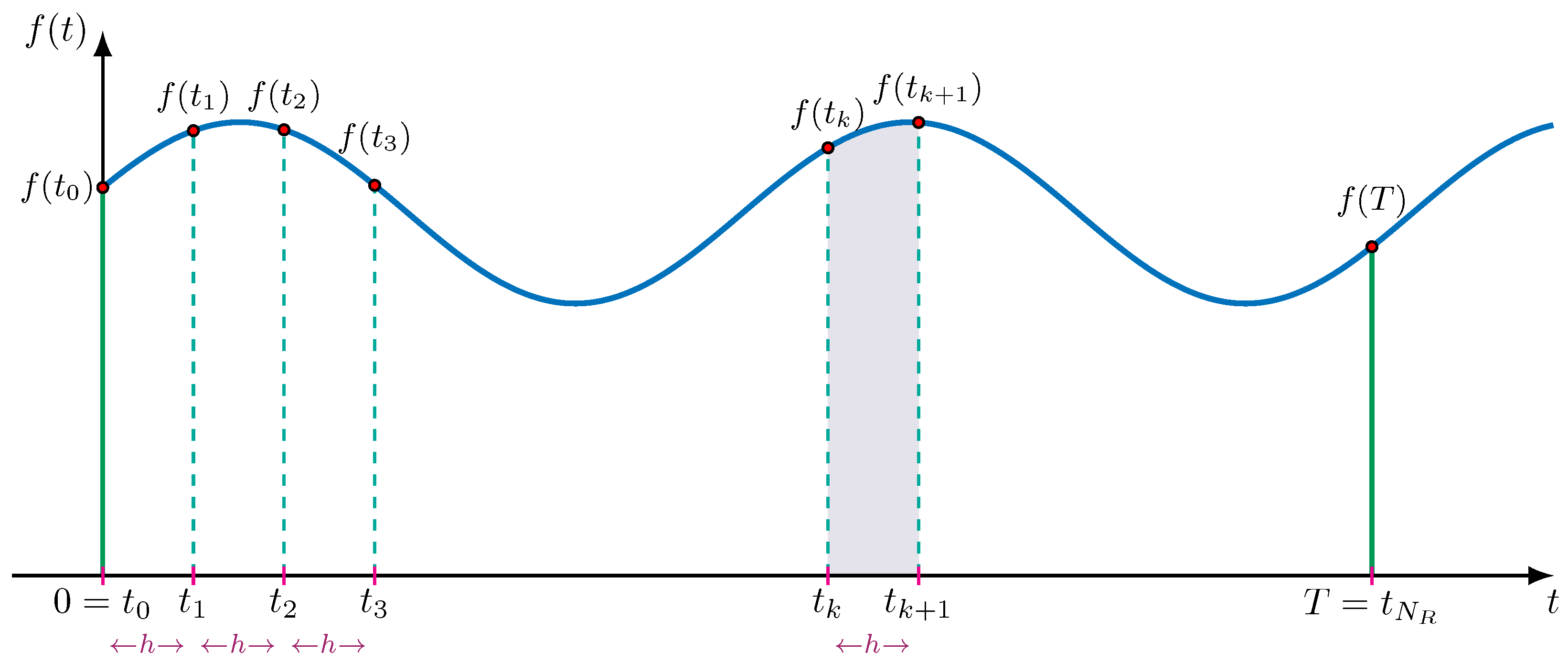
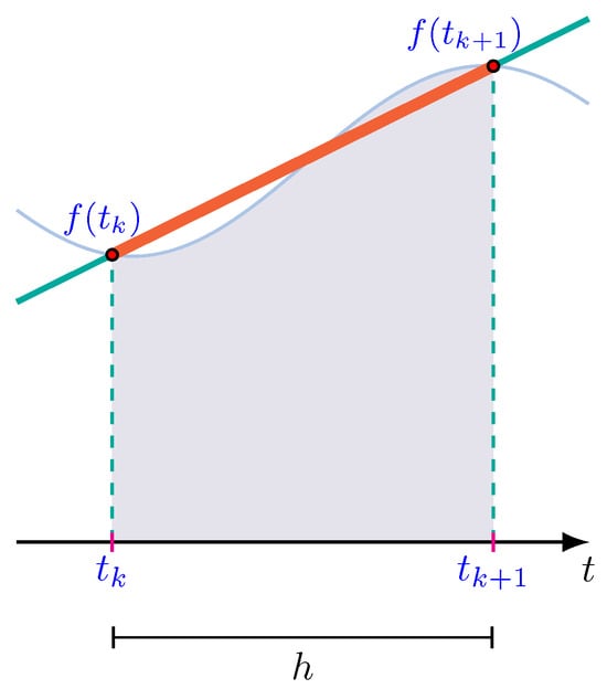
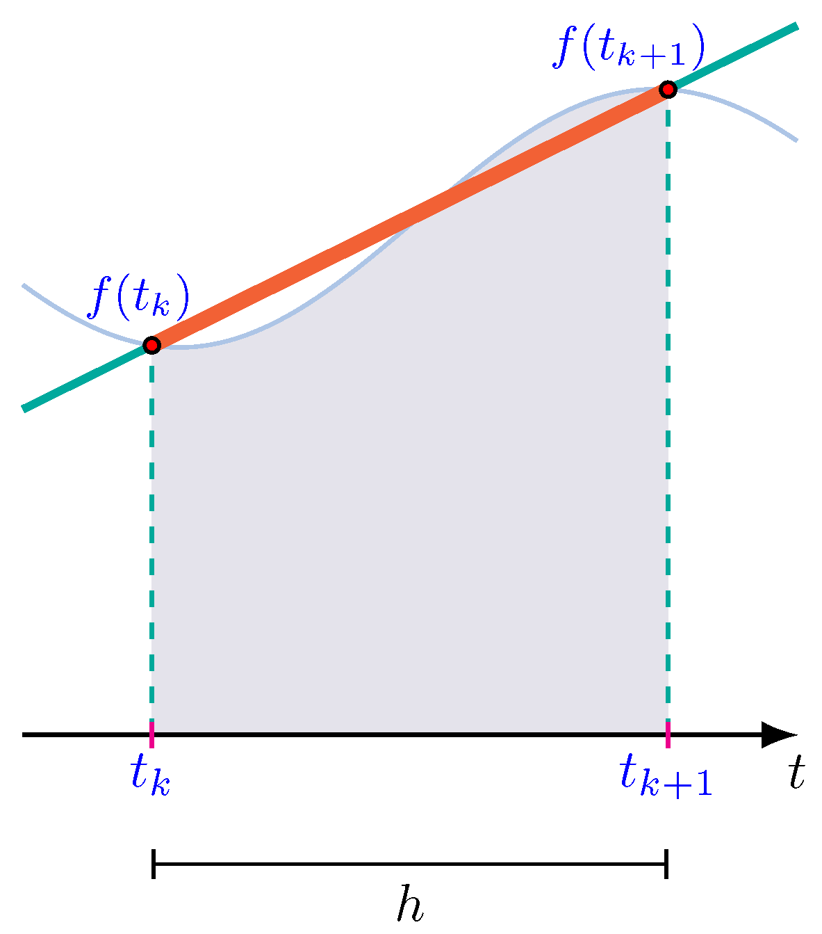
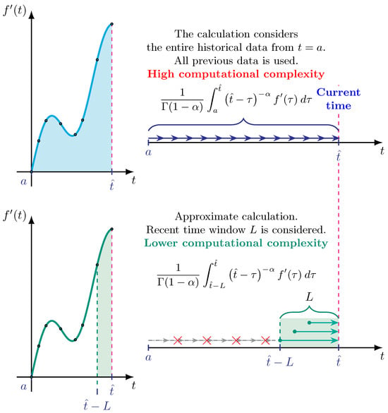
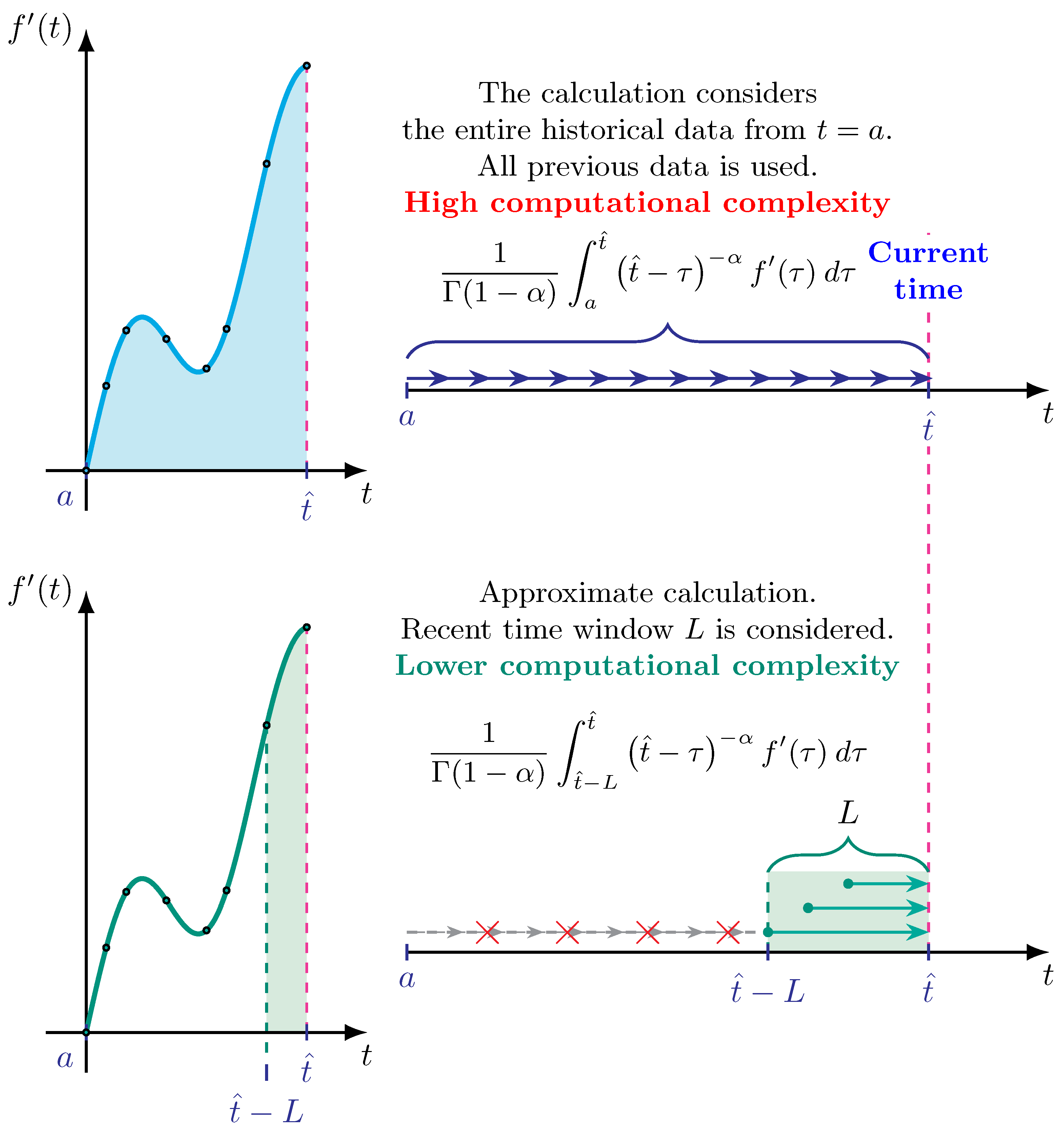
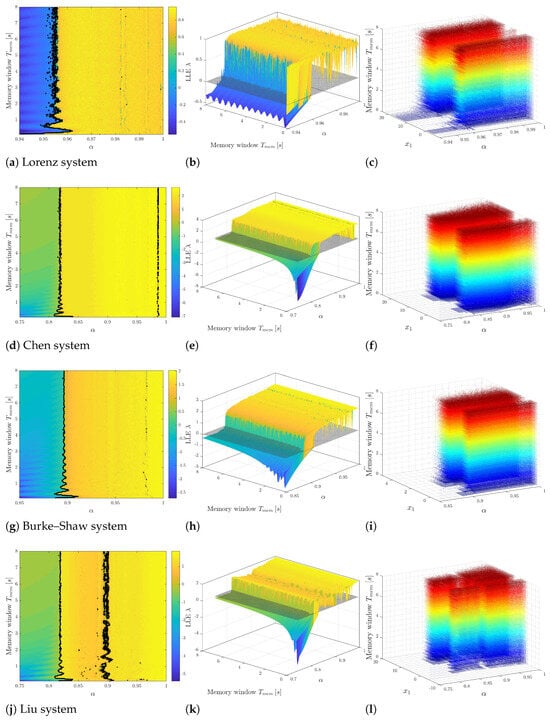
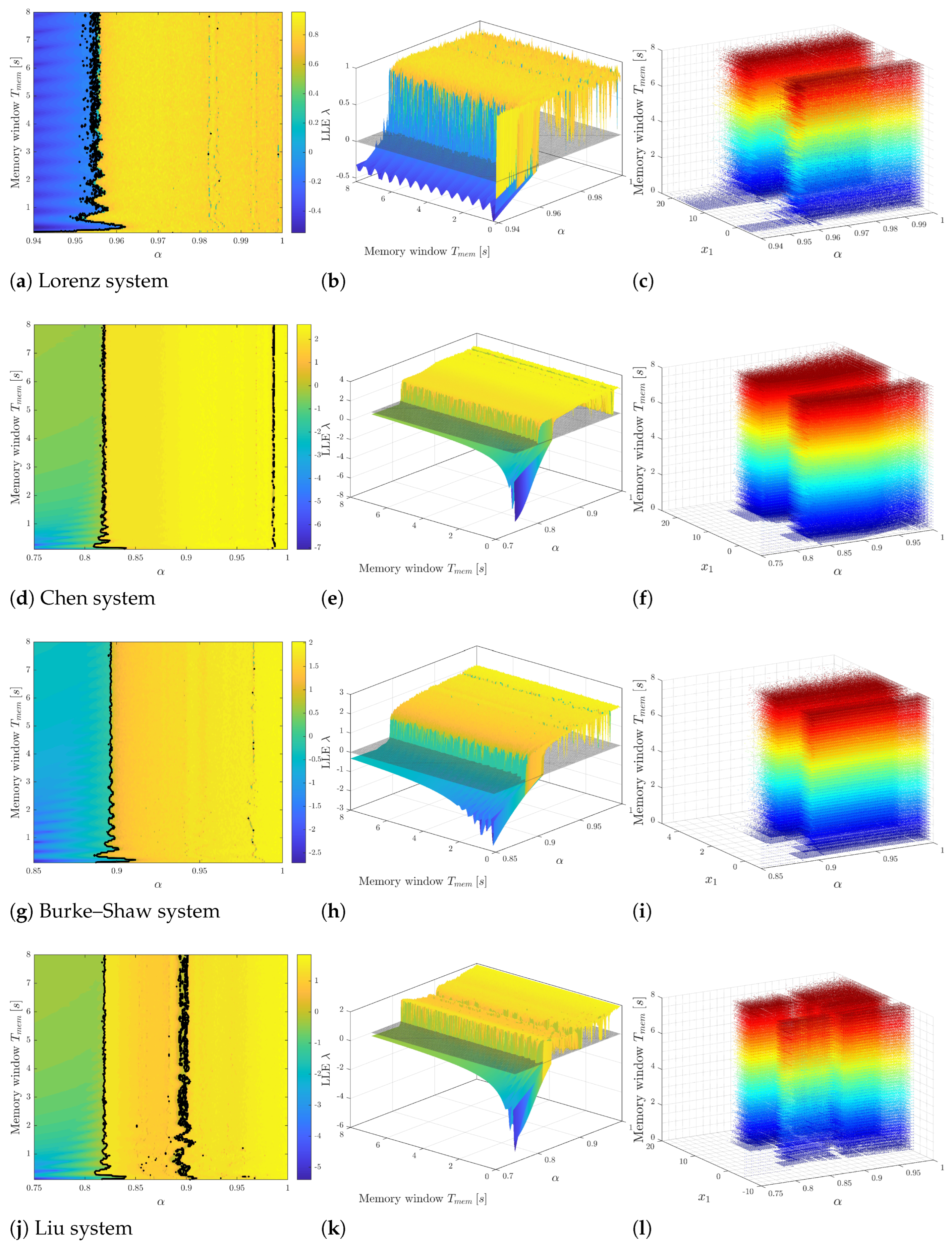
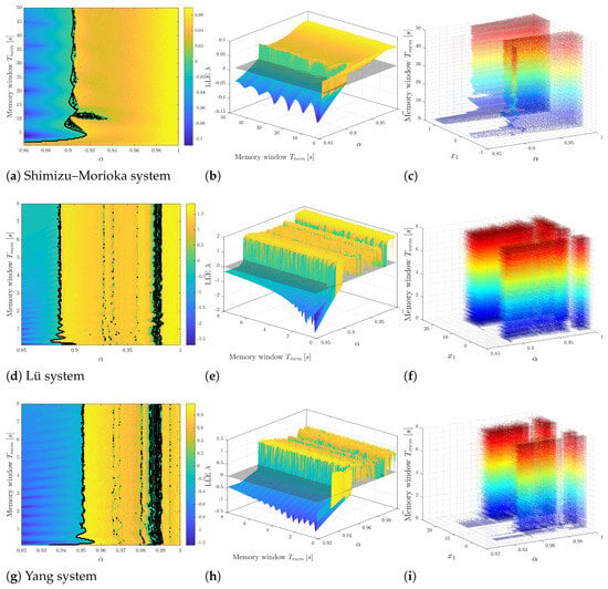
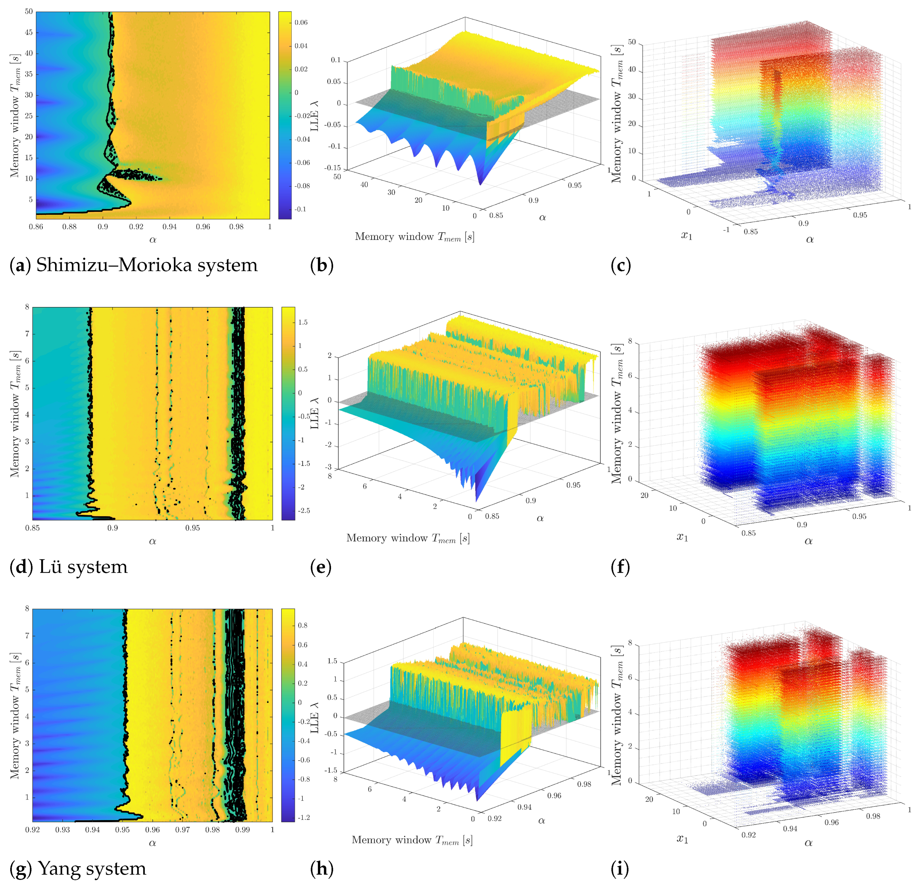
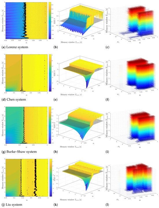
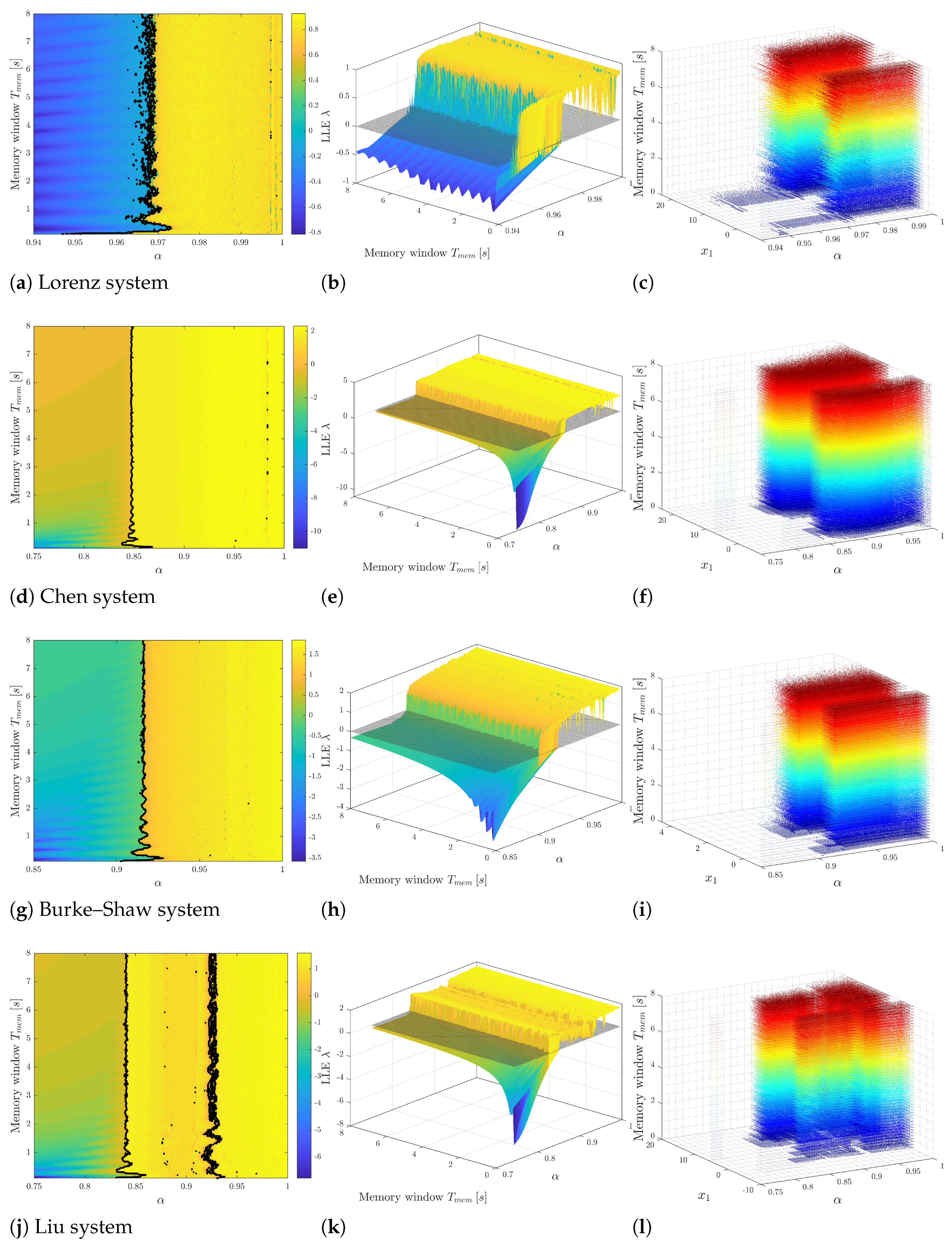
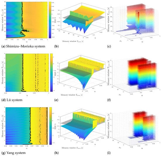
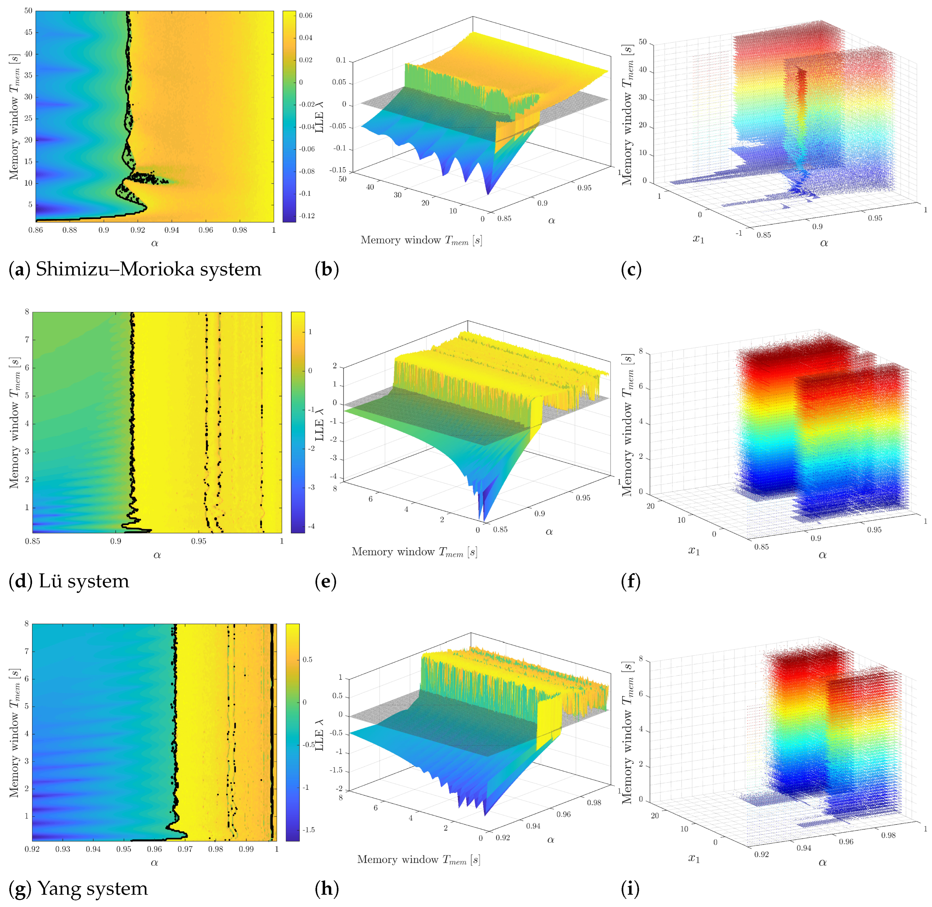
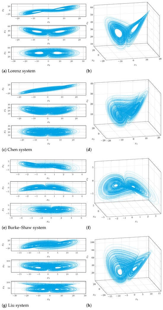
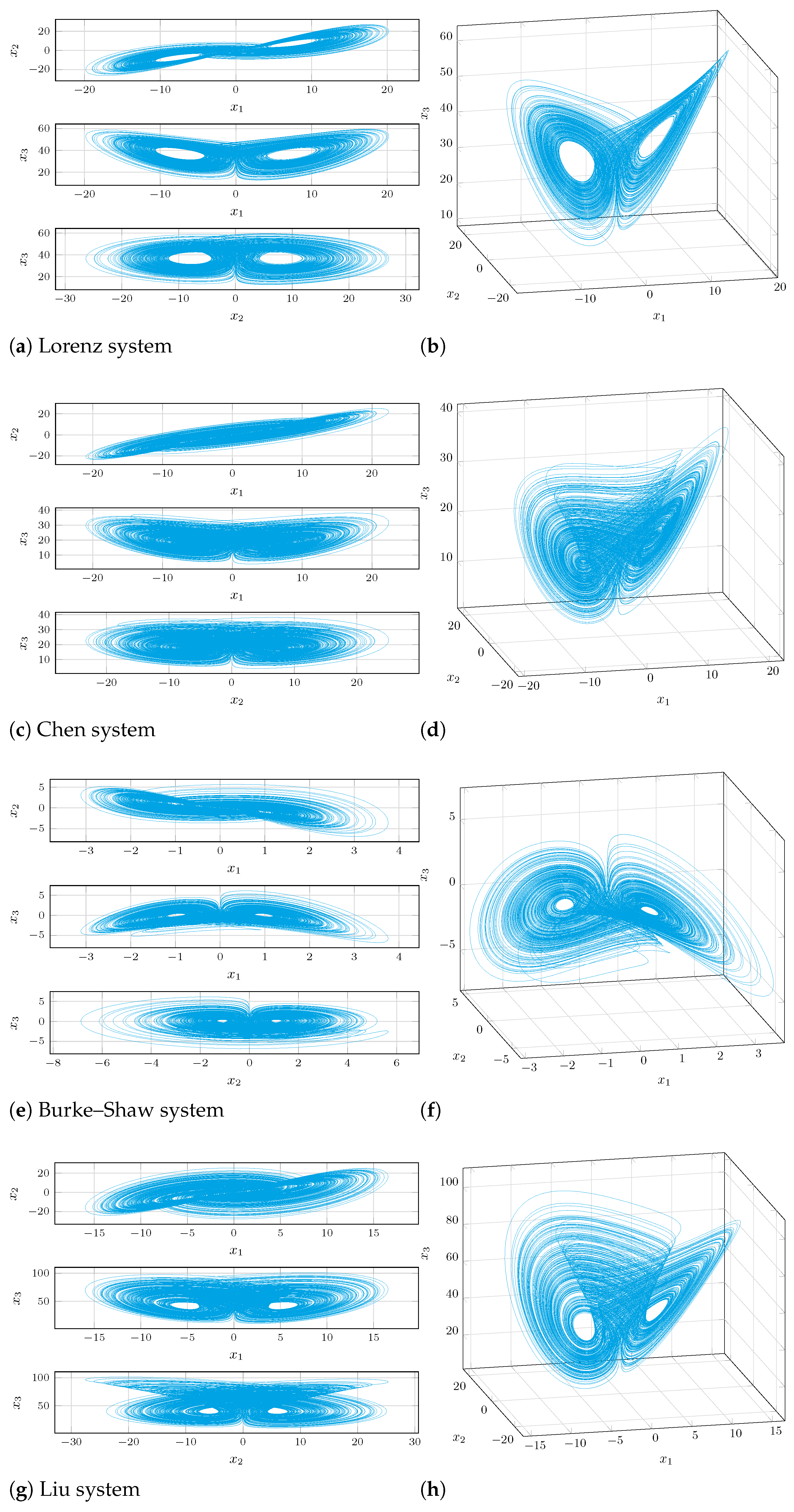
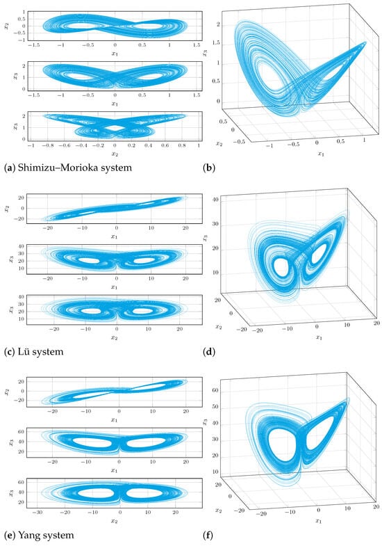
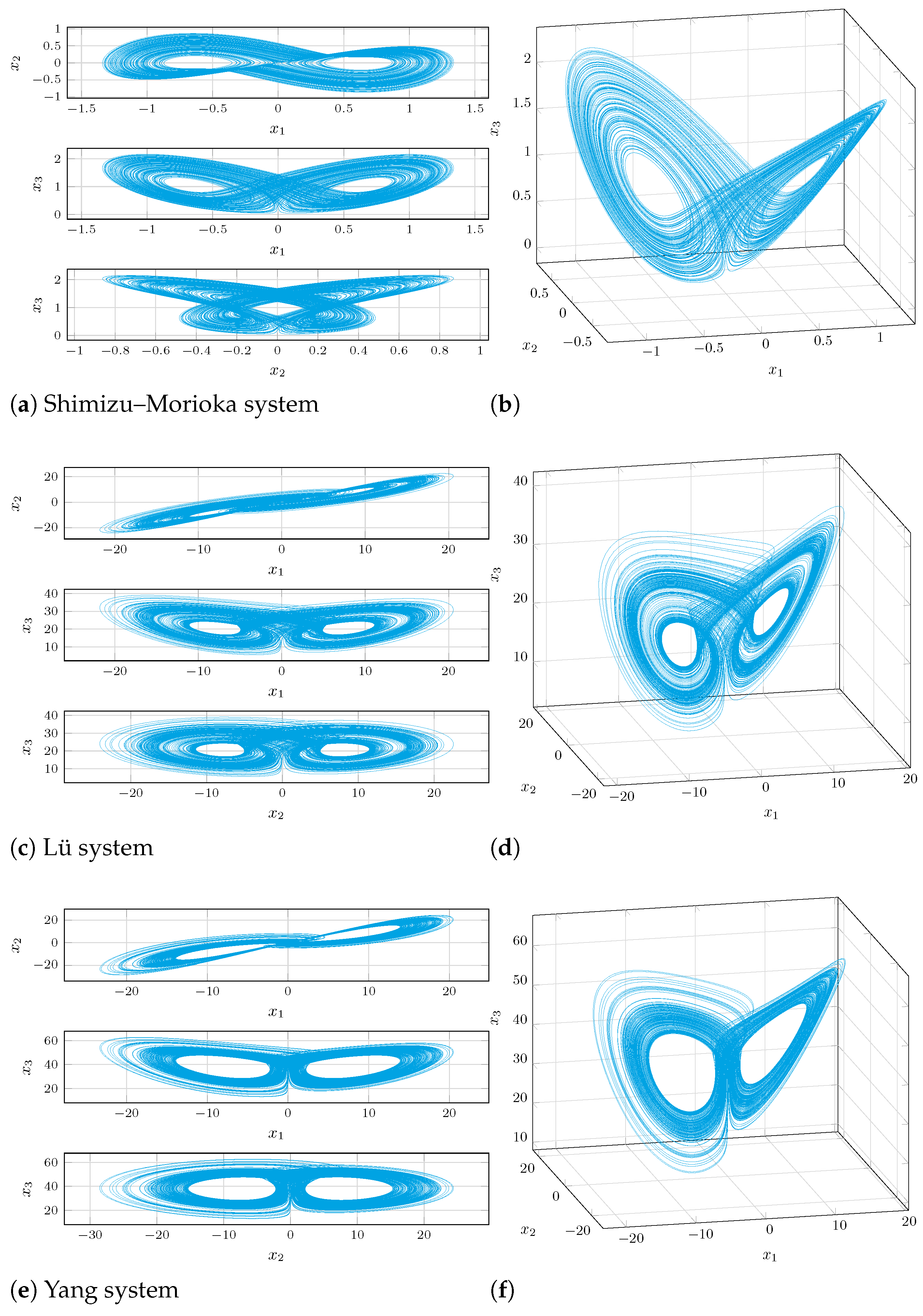
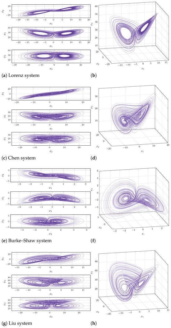
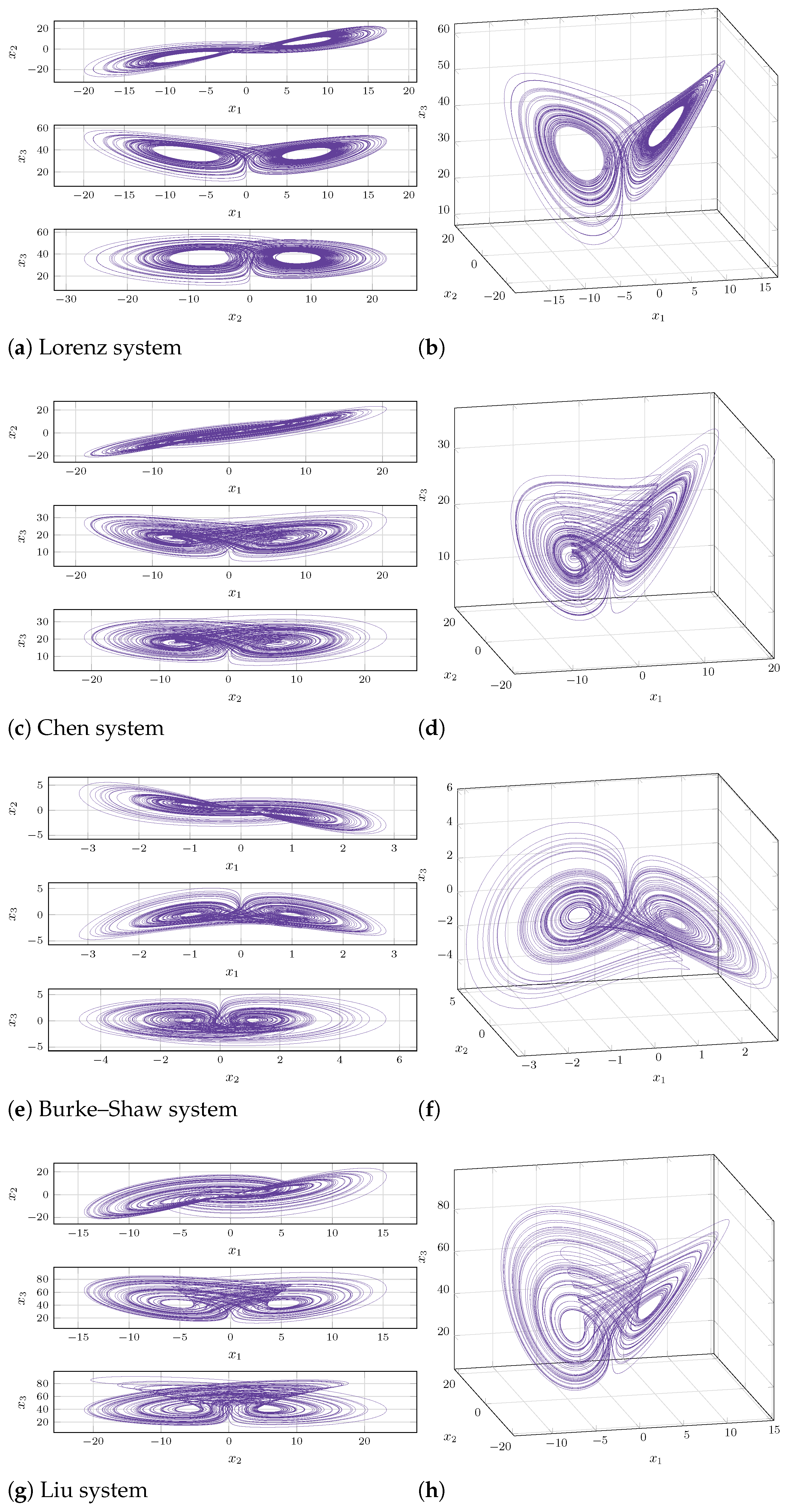
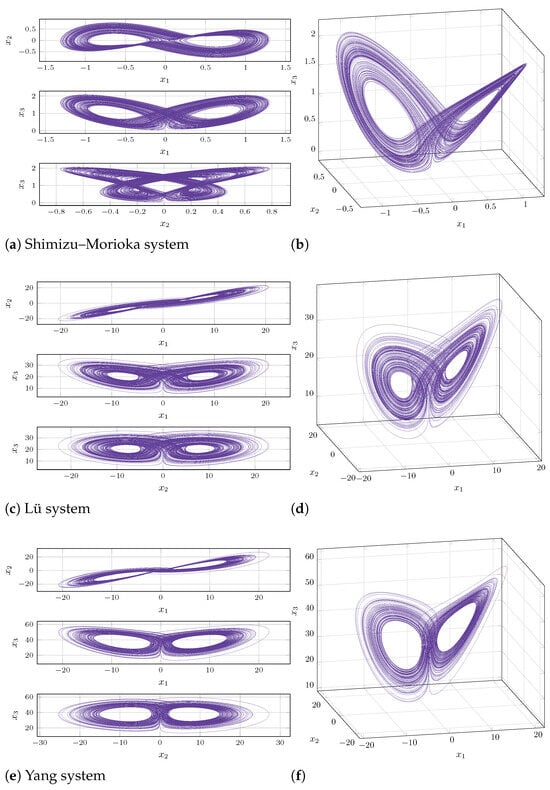
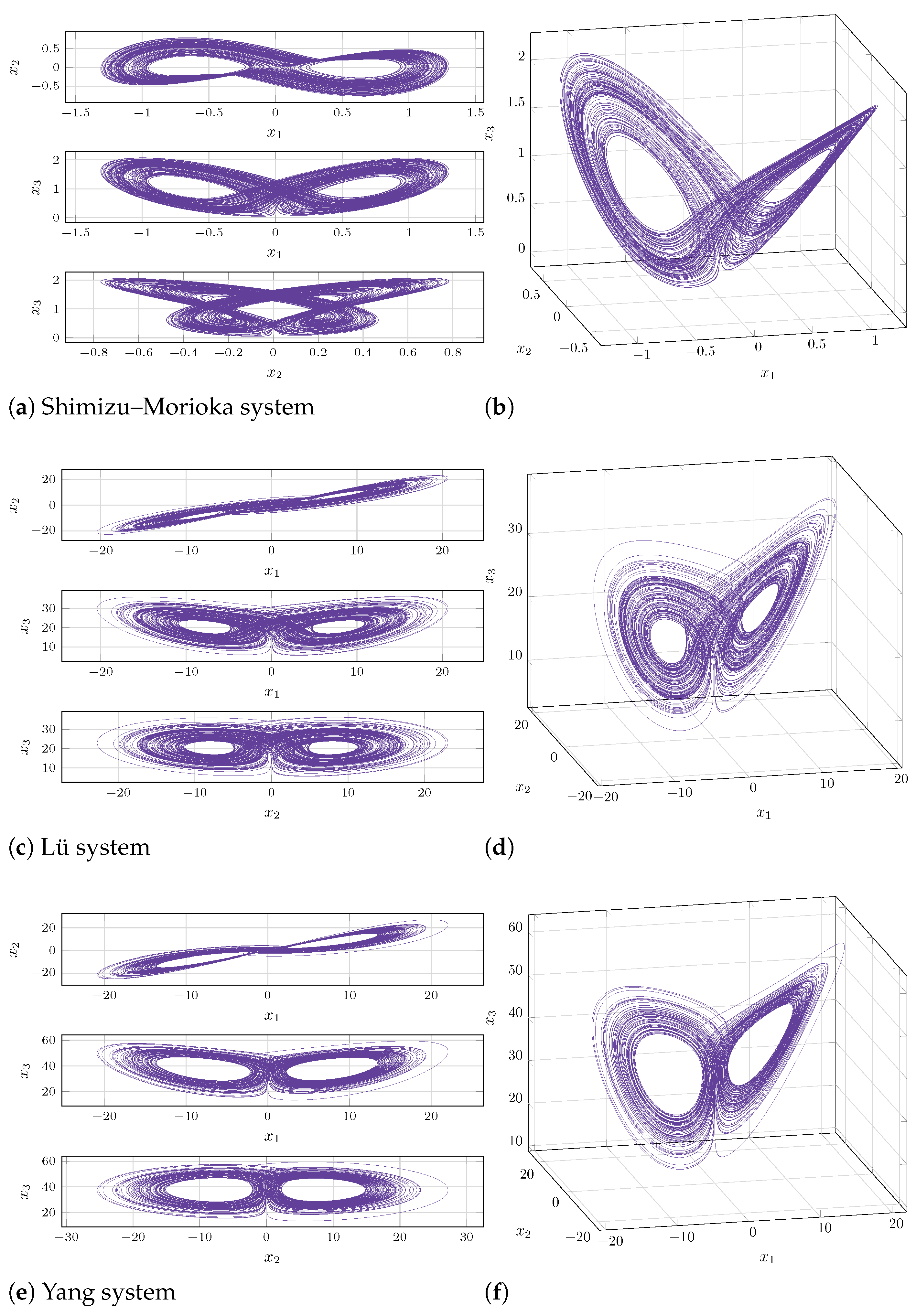
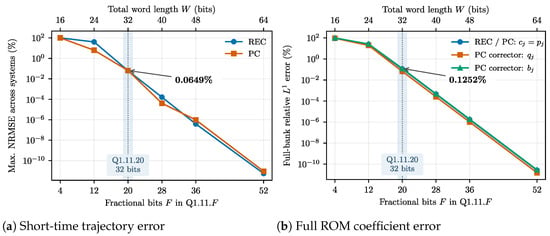
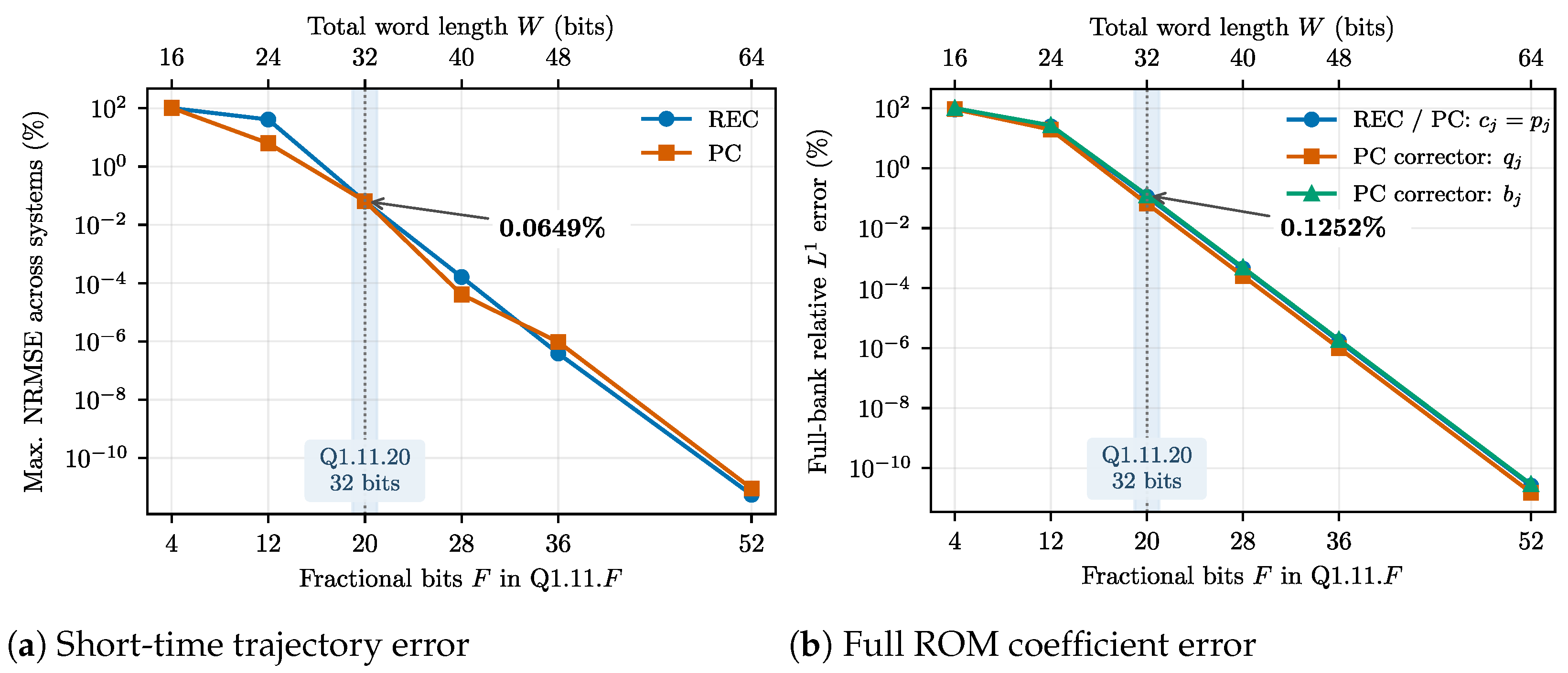
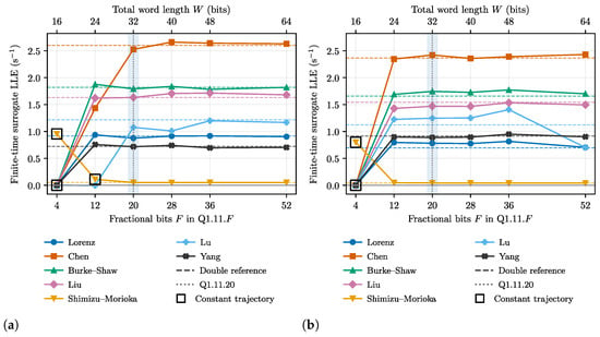
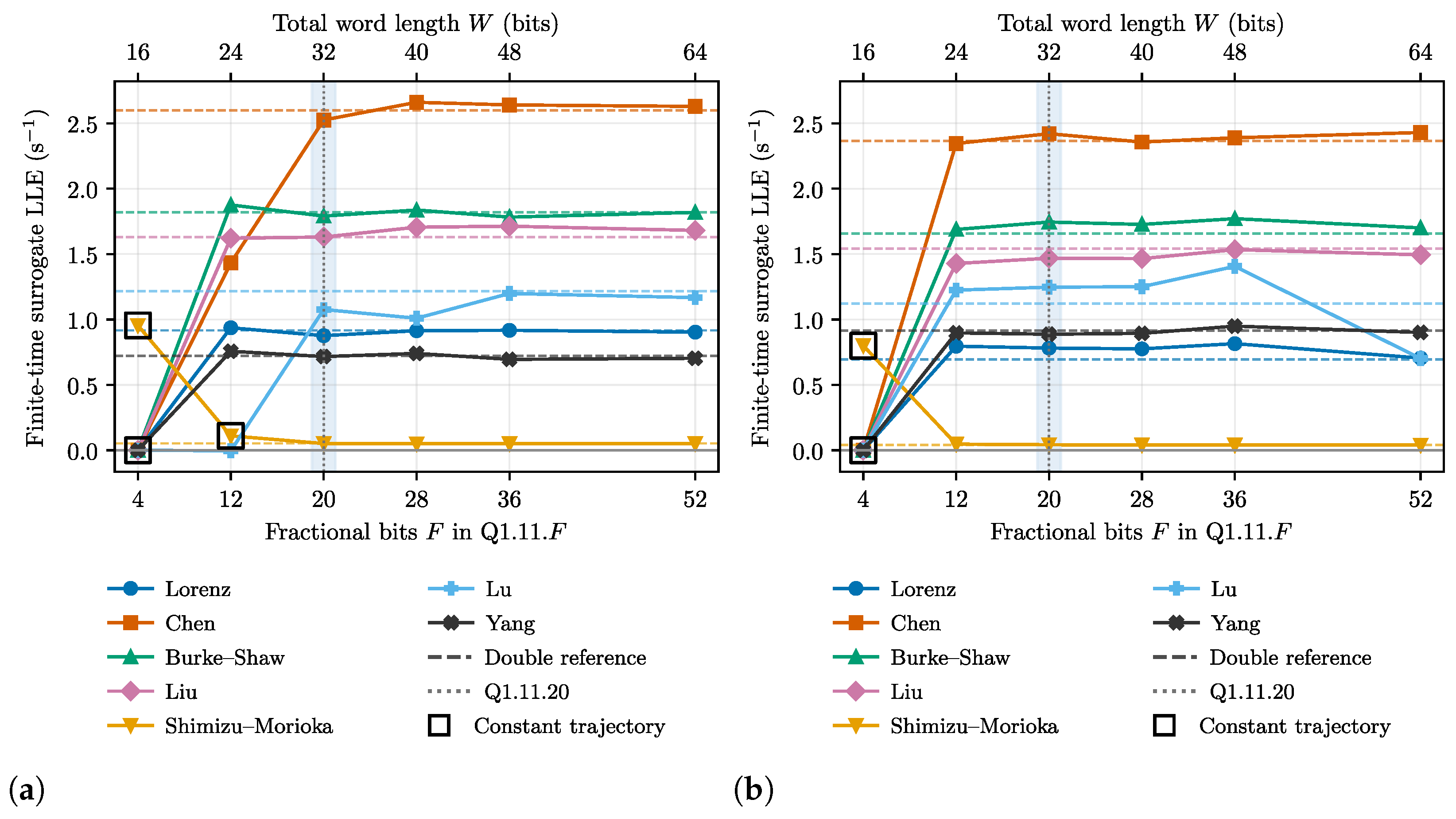
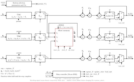
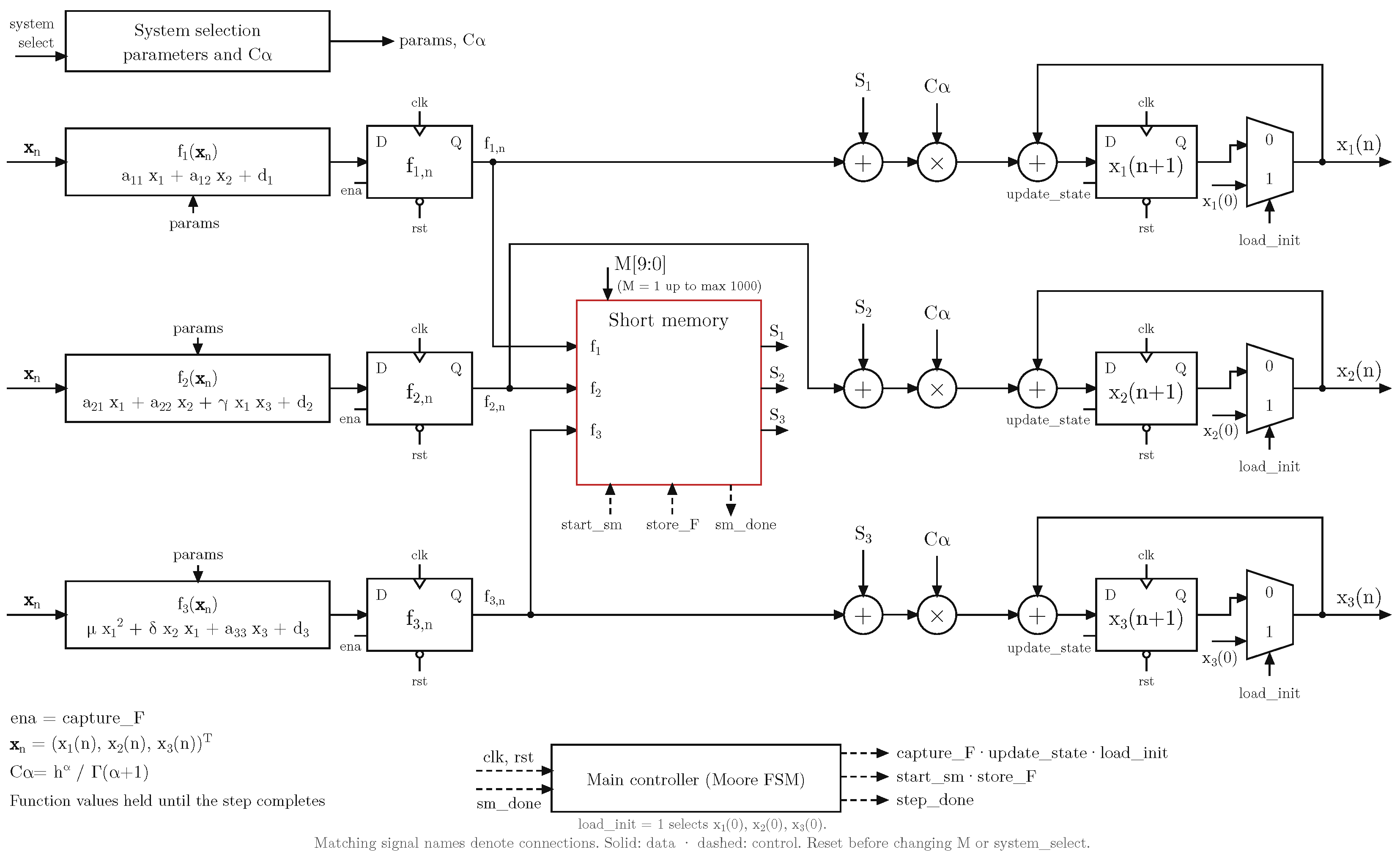
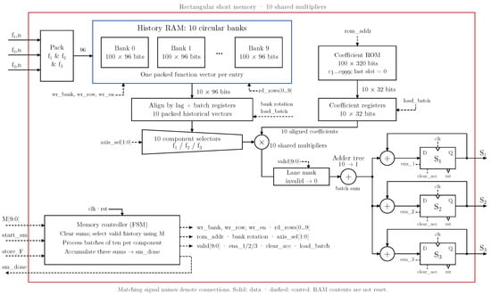
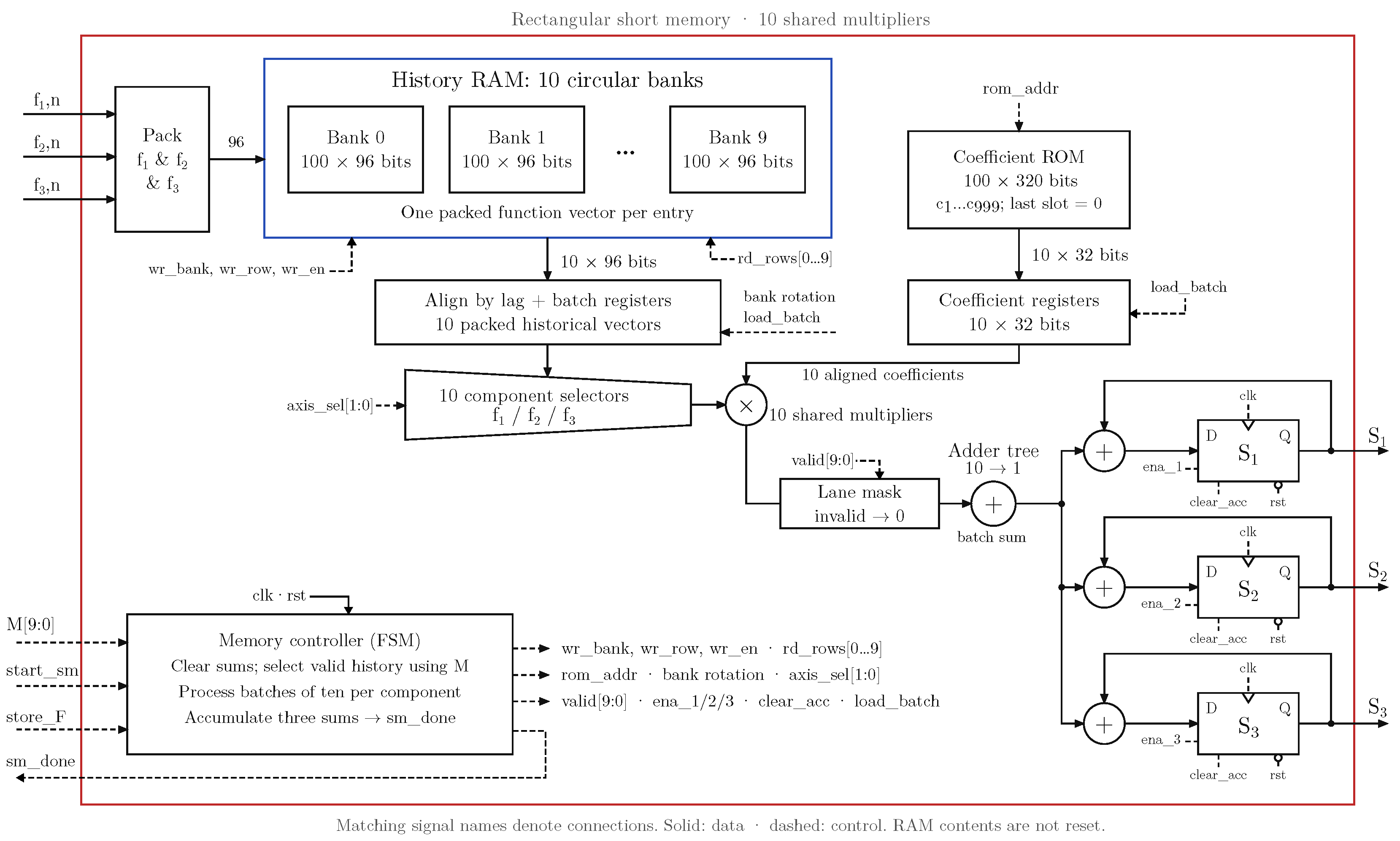
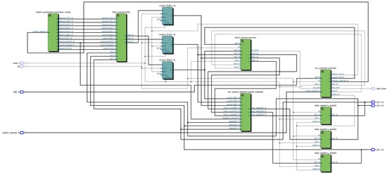
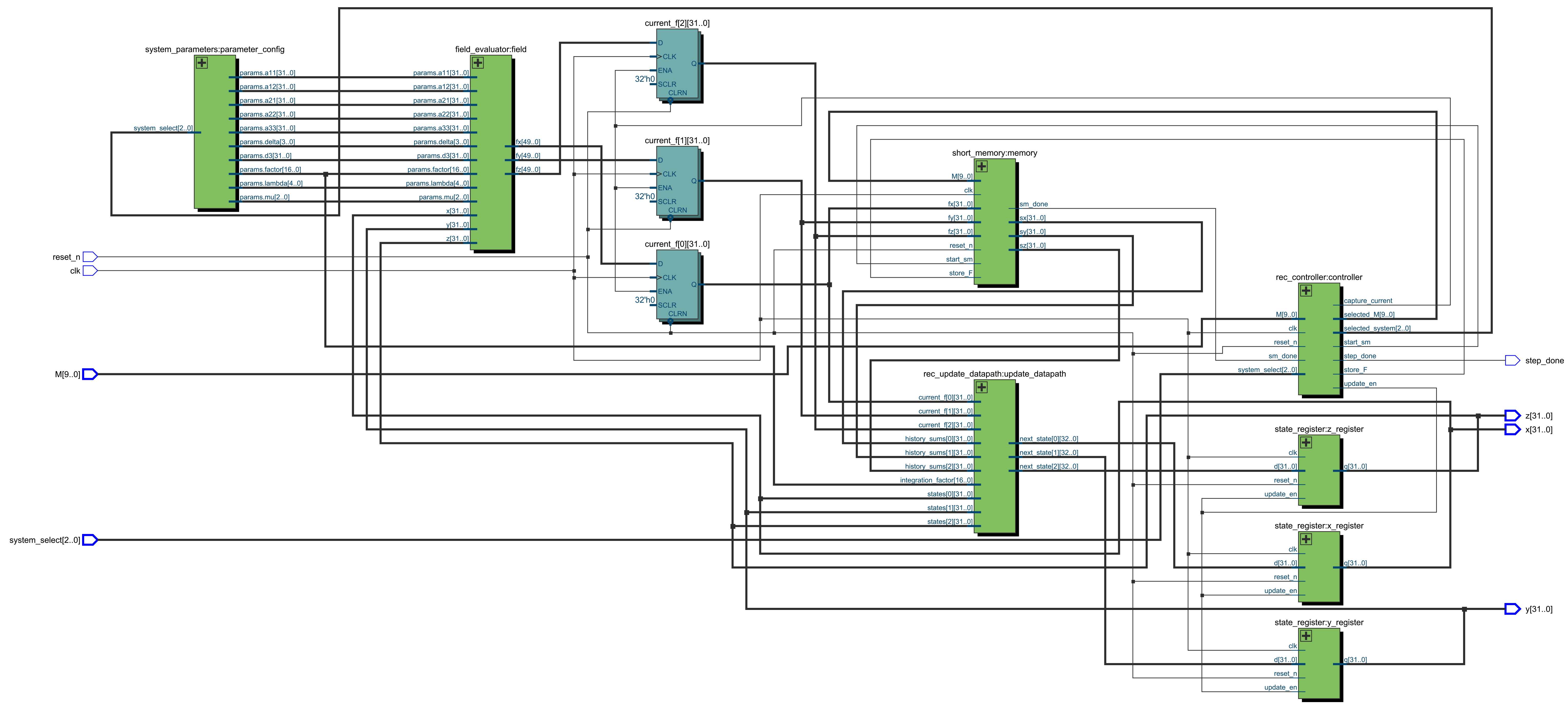
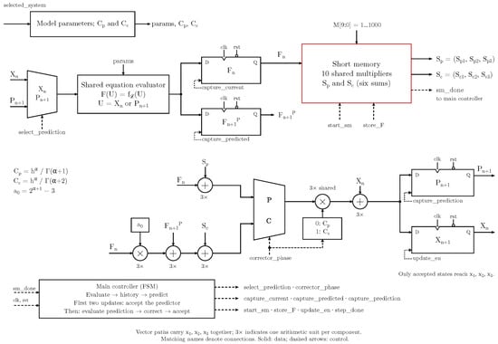
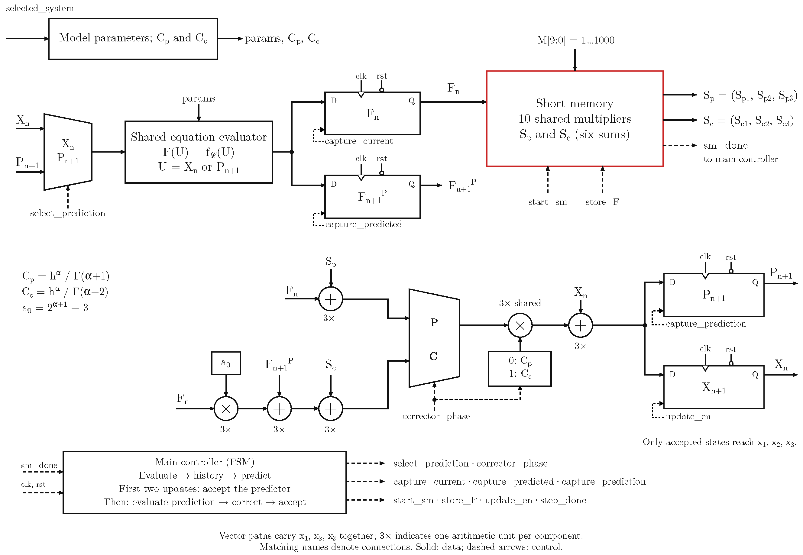
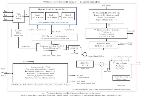
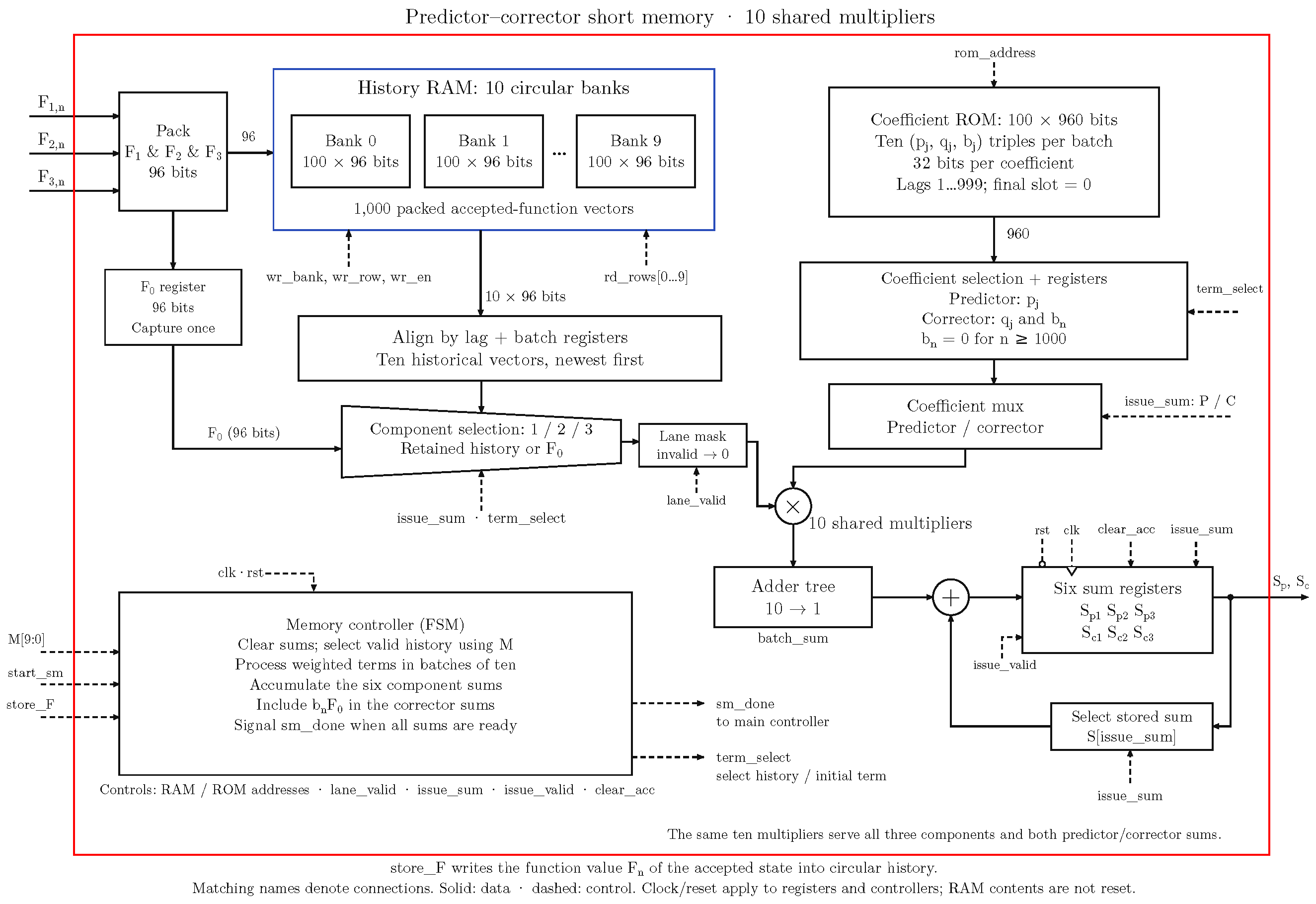
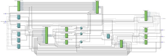
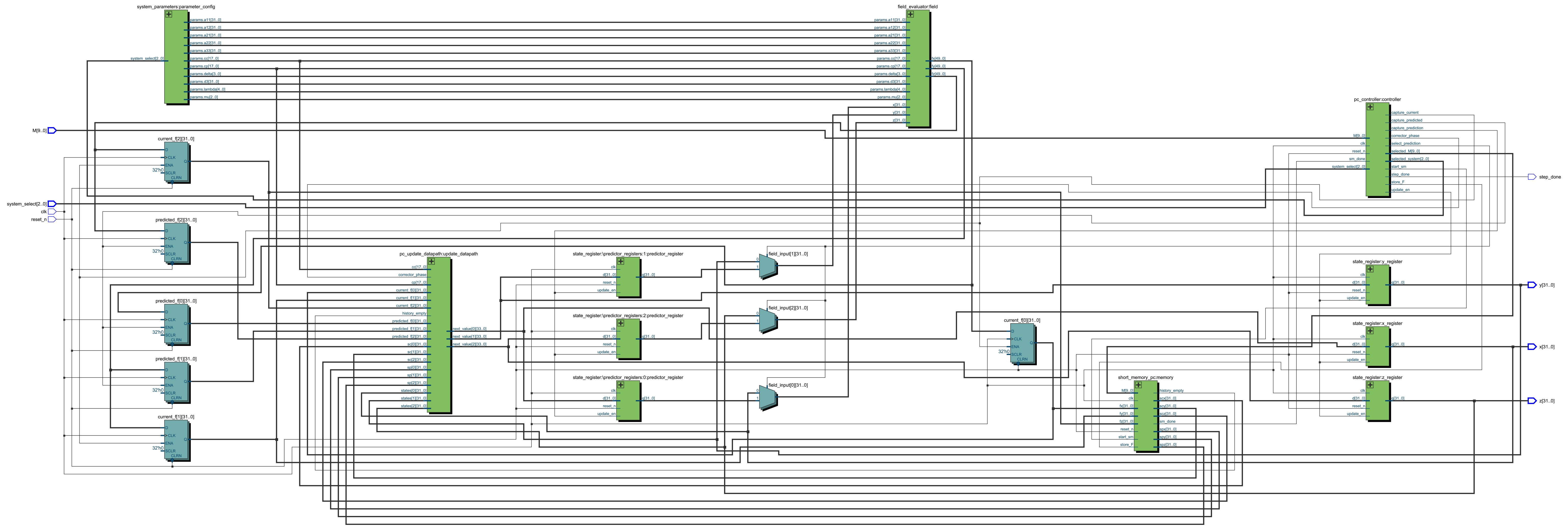
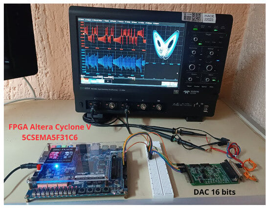
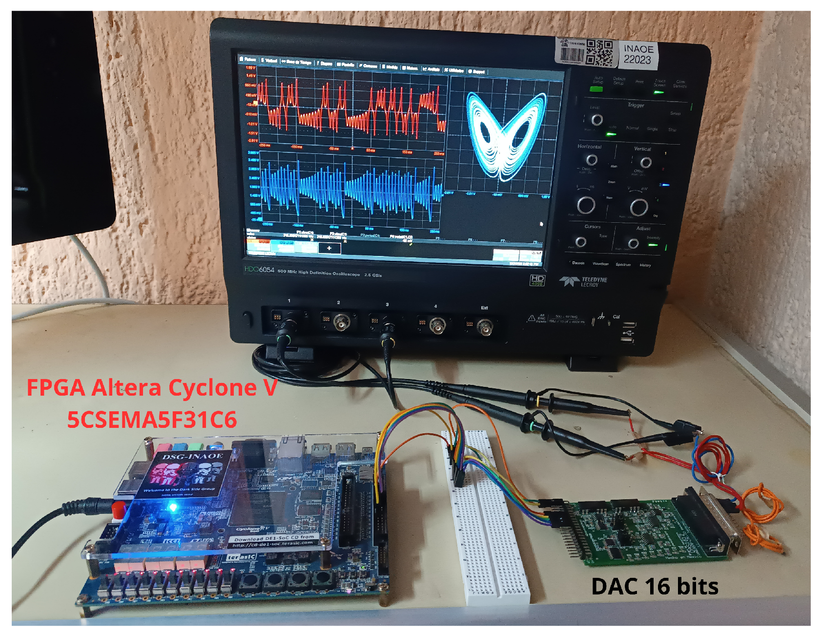
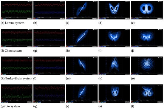
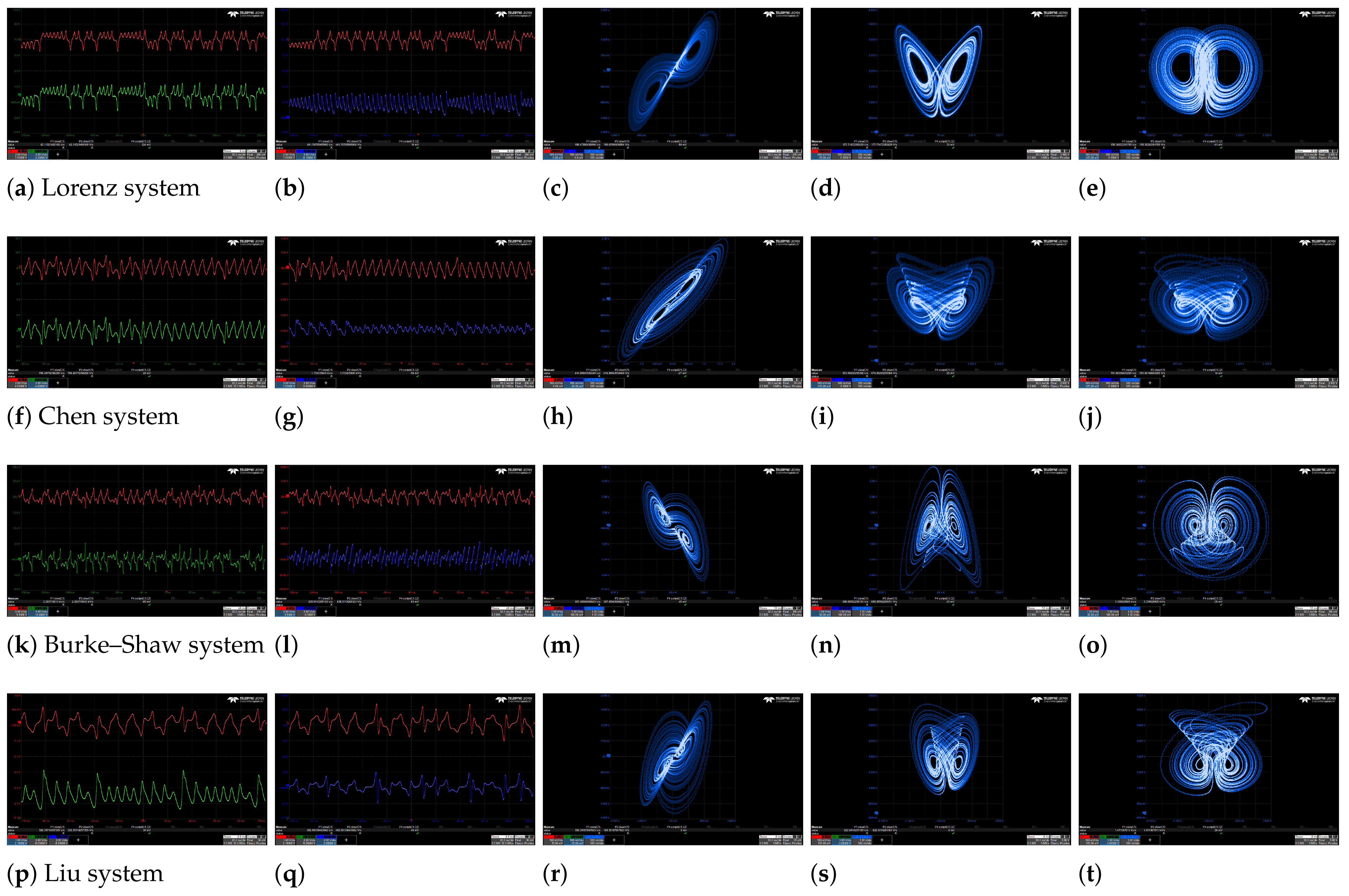
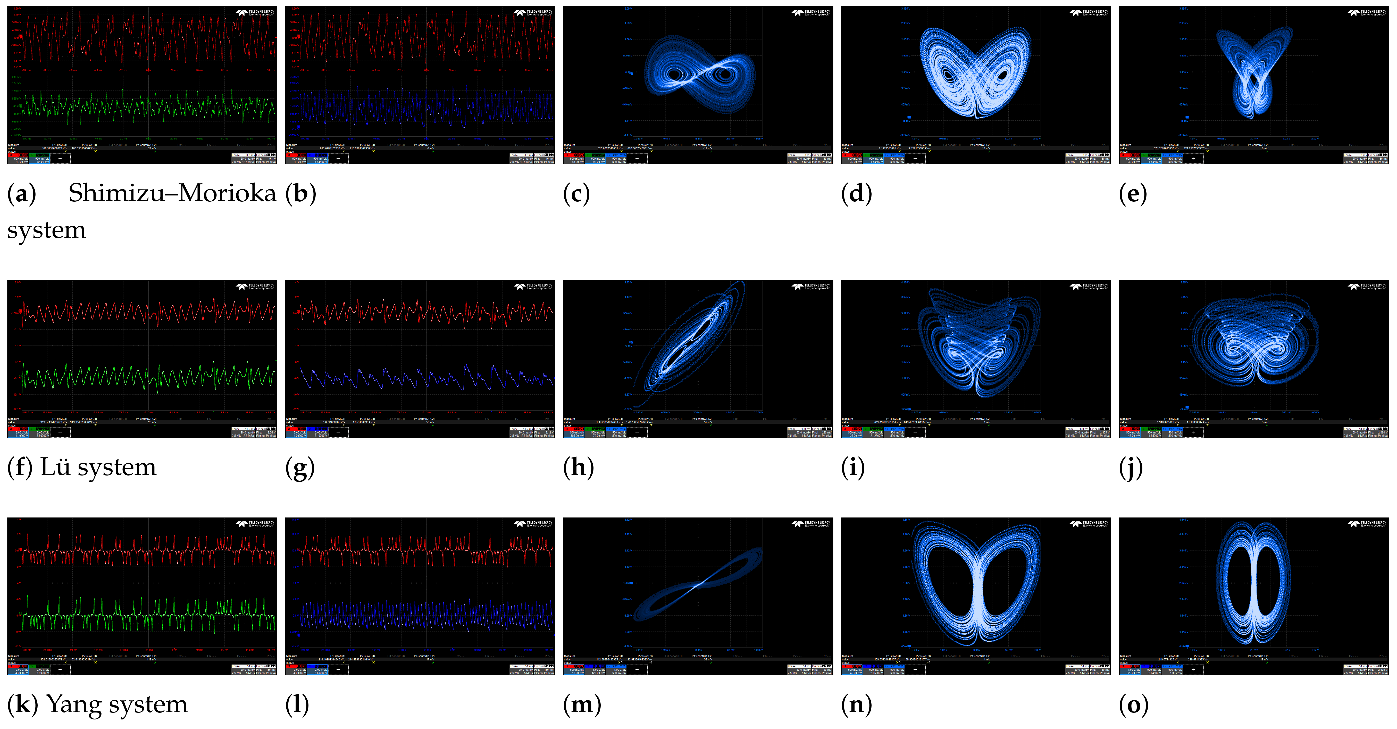
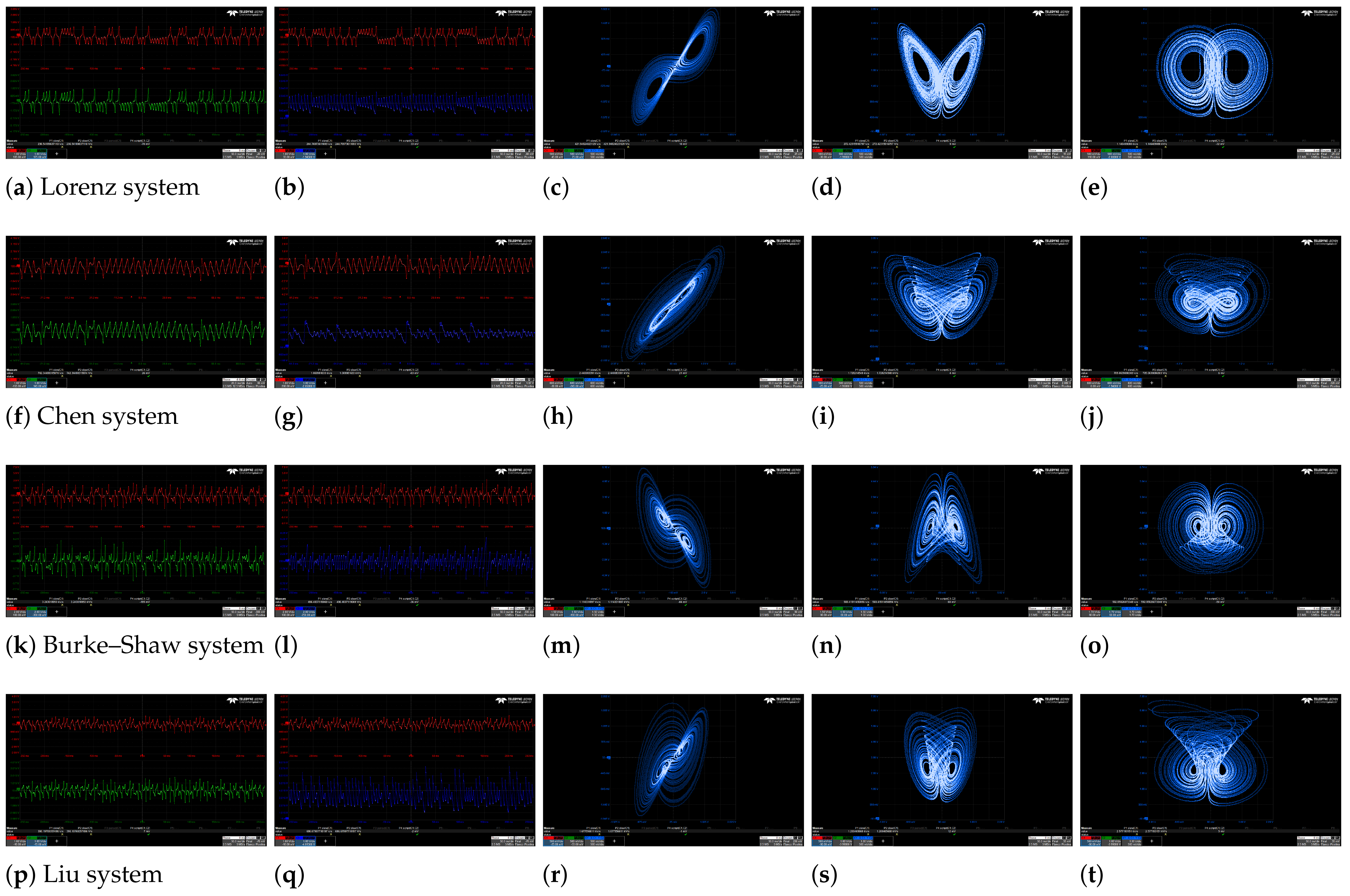
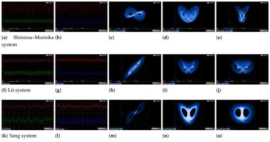
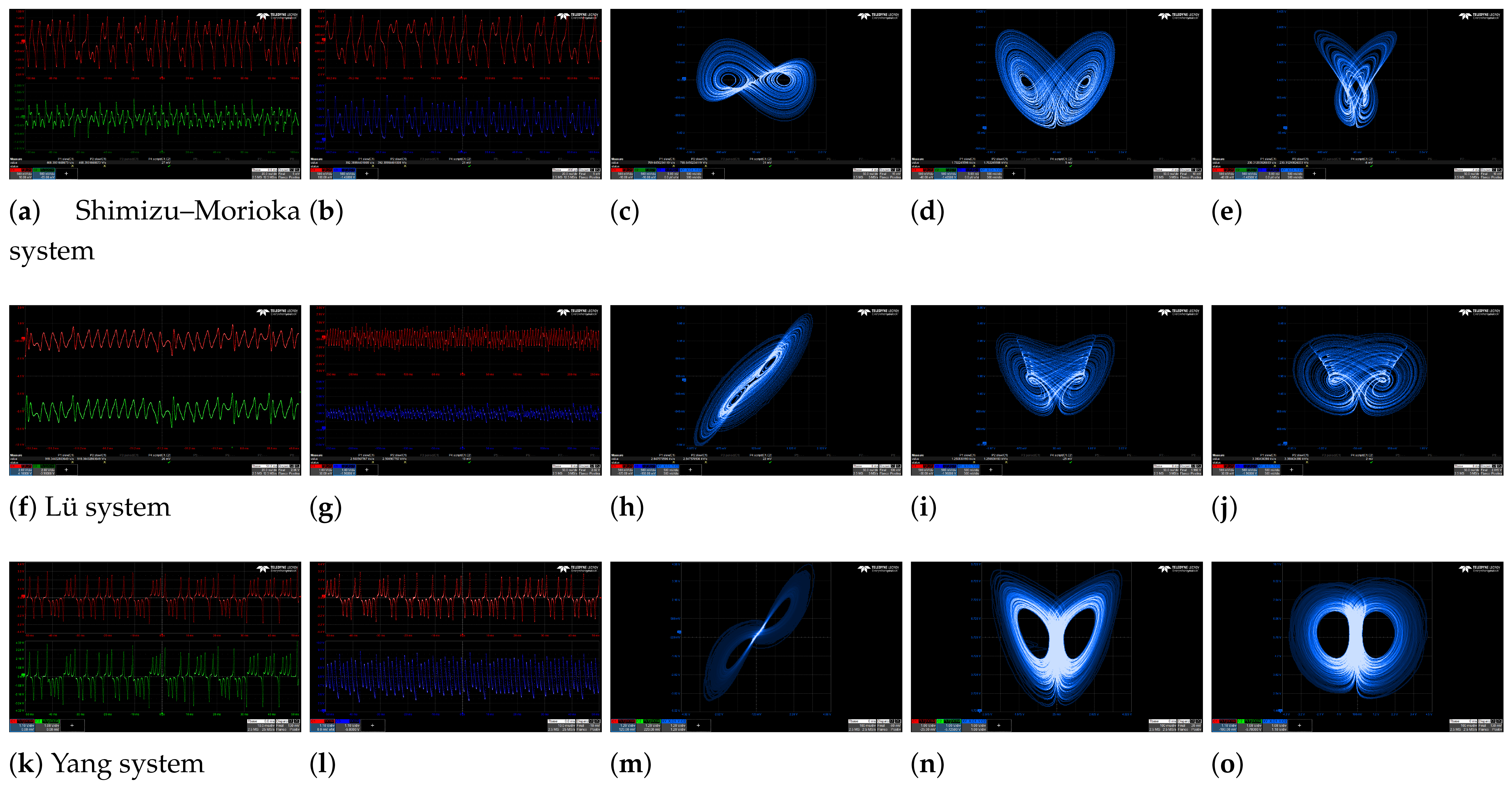
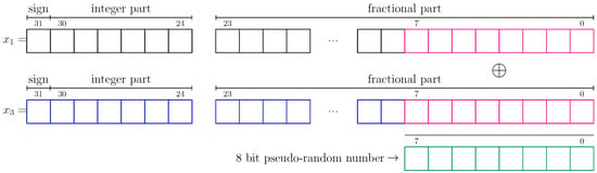
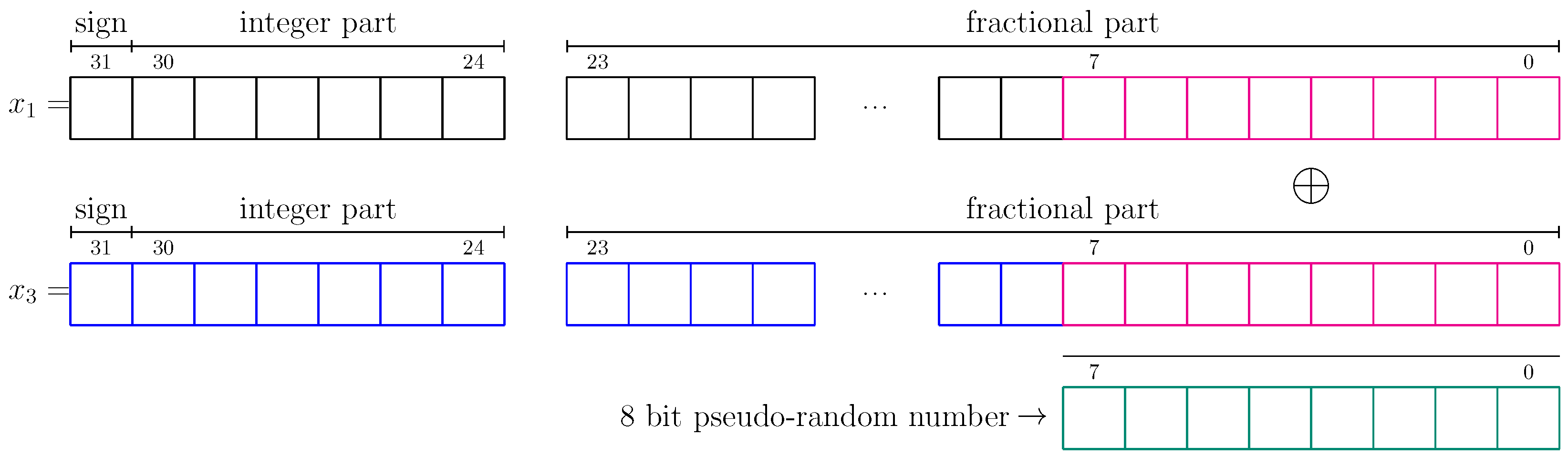

Disclaimer/Publisher’s Note: The statements, opinions and data contained in all publications are solely those of the individual author(s) and contributor(s) and not of MDPI and/or the editor(s). MDPI and/or the editor(s) disclaim responsibility for any injury to people or property resulting from any ideas, methods, instructions or products referred to in the content. |
© 2026 by the authors. Licensee MDPI, Basel, Switzerland. This article is an open access article distributed under the terms and conditions of the Creative Commons Attribution (CC BY) license.