Bicontrolled Contractive Approach to the Existence of Solutions to the Fractional Aizawa Model

Abstract

We introduce a novel class of $(F,B)$-contractions on complete metric spaces by imposing appropriate conditions on the auxiliary functions F and B. A new fixed-point theorem has been established, guaranteeing both the existence and uniqueness of the fixed point. This result brings together and expands upon several traditional contributions in fixed-point theory. The practicality of this theoretical framework is demonstrated through illustrative examples, including the existence and uniqueness of solutions to the fractional-order Aizawa system formulated with the Atangana–Baleanu fractional derivative. Numerical simulations, supported by graphical analysis and Lyapunov exponents, are presented to characterize the system’s dynamical behavior and to validate the effectiveness of the proposed results.

1. Introduction

Fixed-point theory is a useful tool for proving the existence, uniqueness, and convergence of solutions to nonlinear problems. The Banach [1] contraction principle is a key result in this area, but newer developments have expanded on this concept by introducing more flexible control functions and alternative ways of measuring distances between mappings. Researchers such as Rakotch [2], Boyd–Wong [3], Ćirić [4], Reich, Wardowski [5,6], and Proinov [7] have contributed to enlarging the class of contractive mappings that can be considered. These developments are significant not only because they lead to more fixed-point theorems but also because they offer new ways to impose contractive behavior when a uniform Lipschitz constant is not available.

Agarwal et al. [8], Bedre et al. [9], Popescu et al. [10], and Nazam et al. [11] have carried out remarkable work for the advancement of the idea of F-contractions. The use of fixed-point results in solving physical and engineering problems is illustrated in [12,13].

One important extension to consider is the Ćirić–Reich–Rus-type condition, which controls the distance between two images by considering the distance between the original points and the displacement of each point under the mapping simultaneously. This condition offers more flexibility compared to the Banach [1] contraction because it incorporates additional quantities $\mathfrak{D}(x,\mathfrak{Z}(x))$ and $\mathfrak{D}(y,\mathfrak{Z}(y))$ in addition to $\mathfrak{D}(x,y)$. In our current work, we retain this structure but replace linear control with a pair of nonlinear auxiliary functions F and B. Our objective is to explore how a bicontrolled nonlinear relation can expand the contractive framework, rather than introducing another application of a known fixed-point principle.

The reason for this extension is that existing formulations have limitations. In classical Banach [1] and Reich-type conditions, contractivity is expressed through linear combinations of metric distances. Wardowski-type and related F-contractions use an auxiliary function on the distance, while Proinov-type formulations offer more flexibility through generalized control functions. These approaches show that nonlinear control of the metric distance can significantly expand the range of allowable mappings. However, the control of the image distance and the control of the mixed Reich-type expression have not typically been incorporated simultaneously through two independent auxiliary functions in the form considered here.

Motivated by this observation, we are introducing a bicontrolled $(F,B)$-contraction on complete metric spaces. The proposed condition takes the form of

$$F\left[\mathfrak{D}(Tx,Ty)\right]\le B\left({\alpha }_1\mathfrak{D}(x,y)+{\alpha }_2\mathfrak{D}(x,Tx)+{\alpha }_3\mathfrak{D}(y,Ty)\right)$$

Here, F and B are auxiliary functions that must satisfy specific compatibility conditions. F regulates the distance between the images, while B controls the generalized Reich-type combination of the original and displacement distances. This creates a nonlinear two-function control mechanism that distinguishes it from the classical Banach, Reich, or Ćirić–Reich–Rus formulations.

The relation with existing results can be made explicit. When F and B are chosen as identity functions, the proposed condition reduces to a Reich-type contraction. By further suppressing the displacement terms, the Banach contraction is recovered. Moreover, suitable logarithmic choices of F and B yield a Ćirić–Reich–Rus-type condition. Hence, the proposed framework is not disconnected from the classical theory; rather, it contains several established contractive structures as particular cases while allowing a genuinely nonlinear comparison between the two sides of the contractive inequality. This reduction property also clarifies that the novelty lies in the bicontrolled nonlinear formulation rather than in merely renaming an existing contraction.

The distinction from previous applications to fractional differential equations is also important. The use of fixed-point theorems for fractional differential equations, including equations involving the Atangana–Baleanu derivative, is already well established. Therefore, the fractional character of the application is not claimed as the principal theoretical novelty of this work. Instead, the fractional Aizawa system is used as a nonlinear coupled test problem for the proposed fixed-point framework. Previous studies have established existence and uniqueness results for Atangana–Baleanu fractional differential equations using Banach and other generalized fixed-point techniques, demonstrating that the fractional derivative itself does not automatically create a new fixed-point mechanism. The purpose here is to determine whether the proposed bicontrolled contractive condition provides a useful and mathematically distinct criterion for the corresponding nonlinear dynamical system.

This distinction is particularly important for the fractional-order Aizawa model. A recent study used a fixed-point framework to establish criteria for the existence and uniqueness of a chaotic system involving the Atangana–Baleanu derivative. Our approach is different in that we introduce two auxiliary functions and establish a fixed-point principle under conditions on their mutual behavior, rather than imposing a single linear control. Consequently, our work investigates whether the same class of nonlinear fractional systems can be treated within a broader nonlinear bicontrolled framework.

The paper presents three main contributions. First, it introduces a new class of bicontrolled (F,B)-contractions and establishes conditions for the existence and uniqueness of fixed points in complete metric spaces. Second, it clarifies the relationship of the proposed condition with classical contractions by demonstrating how appropriate choices of auxiliary functions recover important special cases. Third, it applies the resulting theorem to the fractional-order Aizawa system with the Atangana–Baleanu derivative and complements the theoretical results with numerical simulations and dynamical diagnostics. Overall, the paper’s primary contribution lies in the development of the bicontrolled contractive framework and its precise relationship with existing fixed-point principles, with the fractional Aizawa model serving as a nontrivial application to demonstrate the framework’s usefulness. The numerical simulations are used to illustrate the system’s behavior in different parameter regimes, rather than as a substitute for the fixed-point proof.

2. Preliminaries

In order to understand our results, it is important to examine some fundamental concepts from the literature. We begin by defining a metric space which is known for its well-defined distance structure. This structure ensures the existence, uniqueness, and convergence of solutions through fixed-point theorems. Moreover, it provides a foundation for analyzing stability and consistency in fractional dynamical systems.

Definition 1. 

Let $\mathcal{A}\ne \varnothing$. A metric is a mapping $\mathfrak{D}:\mathcal{A}\times \mathcal{A}\to [0,\infty )$ that satisfies the following axioms.

• $\mathfrak{D}(x,y)=0$ if and only if $x=y$ for every $x,y\in \mathcal{A}.$
• $\mathfrak{D}(x,y)=\mathfrak{D}(y,x).$
• Triangular inequality, i.e., $[\mathfrak{D}(x,y)+\mathfrak{D}(y,z)]\ge [\mathfrak{D}(x,z)]$, $\mathit{for}\mathit{all}x,y,z\in \mathcal{A}$.

The pair $(\mathfrak{D},\mathcal{A})$ is called a metric space.

Definition 2 

(Complete metric space). Let $(\mathfrak{D},\mathcal{A})$ be a metric space and $\left\{x_n\right\}$ be any Cauchy sequence in $\mathcal{A}$. The space $(\mathfrak{D},\mathcal{A})$ is called a complete metric space, if for every $\epsilon >0$, there exists a positive integer $N_0$ such that

$$\mathfrak{D}(x_n,x)<\epsilon \mathit{for}\mathit{all}n\ge N_0.$$

and $x\in A,$ i.e., every Cauchy sequence in A converges in A.

A complete metric space is essential in fixed-point theory because it guarantees the convergence within the space. The Banach contraction principle heavily depends on completeness to ensure that the limit of successive approximations exists in the space and acts as the unique fixed point. Recall that a sequence may converge outside the given space if it is not complete, potentially resulting in the absence of a fixed point within the domain. Therefore, completeness is a crucial requirement for the validity of numerous fundamental results and iterative methods in fixed-point theory.

Definition 3 

(banach cotraction). Let $(\mathcal{A},\mathfrak{D})$ be a complete metric space. A mapping $T:\mathcal{A}\to \mathcal{A}$ is said to be a Banach [1] contraction, if there exists a constant k such that

$$\mathfrak{D}\left(T(x),T(y)\right)\le k\mathfrak{D}(x,y)),forall x,y\in \mathcal{A}$$

where $0<k<1$

• The Banach contraction principle necessitates a fixed contraction constant $0<k<1$ for all pairs of points. A natural generalization is constructed by Rakotch [2], permitting the contraction factor to be dependent on the distance between the points.

Definition 4 

(Rakotch contraction). Let $\mathcal{A}\ne 0$ be a complete metric space. It is called a Rakotch [2] contraction If there exists a bounded non-negative function α such that

$$\mathfrak{D}\left(T(x),T(y)\right)\le \alpha (\mathfrak{D}\left(x,y))\mathfrak{D}(x,y)\right),x,y\in \mathcal{A}.$$

where $\alpha (t)<1$ for all $t\in [0,\infty ).$ Replacing the multiplicative contraction factor with an auxiliary function that acts directly on the distance results in a further generalization. This gives rise to the concept of Boyd–Wong [3] contraction, which can be defined as follows.

Definition 5 

(Boyd–Wong contraction). Let $\mathcal{A}$ be a complete metric space; a mapping $T:\mathcal{A}\to \mathcal{A}$ is said to be a Boyd–Wong contraction if there exists an auxiliary function $\psi :[0,\infty )\to [0,\infty )$ such that

• ψ is right continuous over $[0,\infty )$.
• $\psi (t)<t$ for every $t\in (0,\infty )$.

and

$$\mathfrak{D}\left(T(x),T(y)\right)\le \psi (\mathfrak{D}\left((x,y)\right),\mathrm{for}\mathrm{all}x,y\in \mathcal{A}.$$

Reich [14] extended the Banach contraction principle by replacing the Lipschitz constant with a linear combination of three metric distances,

$$\mathfrak{D}(T(x),T(y)\le {\alpha }_1\mathfrak{D}(x,y)+{\alpha }_2\mathfrak{D}(x,T(x))+{\alpha }_3\mathfrak{D}(y,T(y)),$$

$\mathrm{for}\mathrm{all}x,y\in \mathcal{A},\mathrm{where}{\alpha }_1,{\alpha }_2,{\alpha }_3\ge 0\mathrm{with}{\alpha }_1+{\alpha }_2+{\alpha }_3<1.$ Proinov [7] later established fixed-point theorems for generalized contractive mappings governed by a pair of auxiliary functions $\psi ,\varphi$ rather than linear coefficients, unifying several earlier results and demonstrating that nonlinear control of the metric distance can expand the range of admissible mappings while preserving the existence and uniqueness of fixed points.

We recall the following useful lemma due to Suzuki [15], which gives a criterion for a sequence to be a Cauchy sequence.

Lemma 1. 

Let the sequence $\left\{x_n\right\}\subset (\mathcal{A},\mathfrak{D})$ be non-Cauchy and satisfy $\mathfrak{D}(x_n,x_{n+1})\to 0$ when $n\to \infty$. Then, for every $\epsilon >0$, there exist two subsequences $\left\{x_{n_k}\right\}$ and $\left\{x_{m_k}\right\}$ of $\left\{x_n\right\}$ such that

$$\mathfrak{D}(x_{n_{k+1}},x_{m_{k+1}})\to {\epsilon }^{+},wheneverk\to \infty .$$

(1)

Moreover, the limiting value remains unchanged when either index is shifted by one, i.e., when $k\to \infty$.

$$\left\{\begin{array}{c}\hfill \mathfrak{D}(x_{n_k},x_{m_k})\to \epsilon \\ \hfill \mathfrak{D}(x_{n_{k+1}},x_{m_k})\to \epsilon \\ \hfill \mathfrak{D}(x_{n_k},x_{m_{k+1}})\to \epsilon \end{array}\right\}.$$

(2)

The following three lemmas contain information about the equivalence between global boundedness, local limit behavior, and sequential characterization.

Lemma 2 

([7]). Let $F:(0,\infty )\to (-\infty ,\infty )$. Then the following conditions are equivalent:

(a)

${\inf }_{\widehat{t}>\epsilon }F(\widehat{t})>-\infty$ for every $\epsilon >0$.

(b)

${\mathrm{lim\; inf}}_{\widehat{t}\to {\epsilon }^{+}}F(\widehat{t})>-\infty$ for every $\epsilon >0$.

(c)

${\lim }_{n\to \infty }F({\widehat{t}}_n)=-\infty$ implies ${\lim }_{n\to \infty }{\widehat{t}}_n=0$.

Lemma 3. 

Let $B:(0,\infty )\to (0,\infty )$. Then the following three conditions are equivalent:

(a)

If ${\lim }_{n\to \infty }{\widehat{t}}_n=\epsilon >0$, then

$$\underset{n\to \infty }{\mathrm{lim\; inf}}B({\widehat{t}}_n)>0.$$

(b)

If ${\lim }_{n\to \infty }B({\widehat{t}}_n)=0$ for a bounded sequence $({\widehat{t}}_n)\subset (0,\infty )$, then

$$\underset{n\to \infty }{\lim }{\widehat{t}}_n=0.$$

(c)

${\mathrm{lim\; inf}}_{\widehat{t}\to {\epsilon }^{+}}B(\widehat{t})>0$ for every $\epsilon >0$.

Proof. 

• Case 1. $((a)\Rightarrow (b))$: Let (a) hold and suppose that ${\lim }_{n\to \infty }B({\widehat{t}}_n)=0$ for a bounded sequence $({\widehat{t}}_n)\subset (0,\infty )$ and the sequence  $({\widehat{t}}_n)$ does not converge to 0. By boundedness, there exist $\epsilon >0$  and a subsequence  $({\widehat{t}}_{n_k})$ such that

  $$\underset{k\to \infty }{\lim }{\widehat{t}}_{n_k}=\epsilon .$$

             Then condition $(a)$ implies

  $$\underset{k\to \infty }{\mathrm{lim\; inf}}B({\widehat{t}}_{n_k})>0,$$

    which contradicts ${\lim }_{n\to \infty }B({\widehat{t}}_n)=0$. Thus, (b) holds.
• Case 2. ($(b)\Rightarrow (c)):$ This follows directly from Lemma 2.  
• Case 3. $((c)\Rightarrow (a)):$ Let (c) hold and suppose that ${\lim }_{n\to \infty }{\widehat{t}}_n=\epsilon >0$. If $(a)$ does not hold, then 

  $$\underset{n\to \infty }{\mathrm{lim\; inf}}B({\widehat{t}}_n)=0,$$

    which contradicts $(c)$. Hence,  $(a)$ holds.

         □

Lemma 4. 

Let $F,B:(0,\infty )\to \mathbf{R}$ be two functions such that

$$\underset{\widehat{t}\to \epsilon }{\mathrm{lim\; sup}}B(\widehat{t})<\underset{\widehat{t}\to \epsilon }{\mathrm{lim\; inf}}F(\widehat{t})\mathit{for}\mathit{any}\epsilon >0.$$

(3)

Suppose that $(F({\widehat{t}}_n))$ and $(B({\widehat{t}}_n))$ are two sequences; for any bounded sequence $({\widehat{t}}_n)\subset (0,\infty )$, both converge to the same limit. Then

$$\underset{n\to \infty }{\lim }{\widehat{t}}_n=0.$$

Proof. 

Assume, on the contrary, that $({\widehat{t}}_n)$ does not converge to zero. Since $({\widehat{t}}_n)$ is bounded, there exist $\epsilon >0$ and a subsequence $({\widehat{t}}_{n_k})$ such that

$${\widehat{t}}_{n_k}\to \epsilon \mathrm{as}k\to \infty .$$

Then

$$\underset{\widehat{t}\to \epsilon }{\mathrm{lim\; inf}}F(\widehat{t})\le \underset{k\to \infty }{\lim }F({\widehat{t}}_{n_k})=\underset{k\to \infty }{\lim }B({\widehat{t}}_{n_k})\le \underset{\widehat{t}\to \epsilon }{\mathrm{lim\; sup}}B(\widehat{t}),$$

which contradicts condition (3). Hence, we must have

$${\widehat{t}}_n\to 0\mathrm{as}n\to \infty .$$

□

3. Problem Statement

Banach [1] established the following leading fixed-point result.

Theorem 1. 

Ref. [1] Let $\mathcal{A}$ be a complete metric space and $\mathfrak{Z}$ be a contraction over $\mathcal{A}$, that is, there exists a constant $\mathsf{\lambda }\in [0,1)$ such that

$$\mathfrak{D}\left(\mathfrak{Z}(x),\mathfrak{Z}(y)\right)\le \mathsf{\lambda }\left[\mathfrak{D}(x,y)\right]\mathit{for}\mathit{all}x,y\in \mathcal{A}.$$

(4)

Then $\mathfrak{Z}$ admits a unique fixed point in $\mathcal{A}$.

According to a remarkable result by Reich [14], if we exchange the right-hand side of inequality (4) with

$${\alpha }_1\mathfrak{D}(x,y)+{\alpha }_2\mathfrak{D}(x,\mathfrak{Z}x)+{\alpha }_3\mathfrak{D}(y,\mathfrak{Z}y),$$

Theorem 1 remains true. Boyd–Wong [3] presented a leading generalization of Theorem 1 as follows.

Theorem 2. 

Let $(\mathcal{A},\mathfrak{D})$ be a complete metric space and $\mathfrak{Z}:\mathcal{A}\to \mathcal{A}$ be a self-mapping that satisfies the following contractive condition:

$$\mathfrak{D}(\mathfrak{Z}x,\mathfrak{Z}y)\le \psi (\mathfrak{D}(x,y))\mathit{for}\mathit{all}x,y\in \mathcal{A},$$

where $\psi :[0,\infty )\to [0,\infty )$ meets the following conditions:

(i)

$\psi (\widehat{t})<\widehat{t}$ for all $\widehat{t}>0$.

(ii)

${\mathrm{lim\; sup}}_{t\to {\widehat{t}}^{+}}\psi (t)<\widehat{t}$ for all $\widehat{t}>0$.

Then $\mathfrak{Z}$ has a unique fixed point and the iterative sequence $({\mathfrak{Z}}^{n}x)$ converges to a fixed point for all $x\in \mathcal{A}$.

Recently, Proinov [7] extended the idea of Boyd–Wong [3] and Wardowski [6]. In this paper, we work on a generalization of Proinov’s [7] idea and hence investigate a mapping $\mathfrak{Z}:\mathcal{A}\to \mathcal{A}$ that satisfies the following generalized contractive condition. We will name such mapping $\mathfrak{Z}$ an $(F,B)$-contraction.

$$F\left[\mathfrak{D}(\mathfrak{Z}x,\mathfrak{Z}y)\right]\le B\left({\alpha }_1\mathfrak{D}(x,y)+{\alpha }_2\mathfrak{D}(x,\mathfrak{Z}x)+{\alpha }_3\mathfrak{D}(y,\mathfrak{Z}y)\right)\mathrm{for}\mathrm{all}x,y\in \mathcal{A}$$

(5)

with $\mathfrak{D}(\mathfrak{Z}x,\mathfrak{Z}y)>0$, where $F,B:(0,\infty )\to (-\infty ,\infty )\mathrm{are}\mathrm{functions},{\alpha }_1,{\alpha }_2\in (0,1),0<{\alpha }_1+{\alpha }_2<1$ and ${\alpha }_3\le 1-({\alpha }_1+{\alpha }_2)$.

We are interested to investigate some useful conditions that lead to the existence and uniqueness of a fixed point of $\mathfrak{Z}$. We demonstrate that the operator associated with a fractional Aizwa model satisfying (5) admits a solution. We also show that an iterative scheme subject to (5) converges to a fixed point. Moreover, we discuss the cases where an iterative scheme associated with the fractional Aizwa model diverges. The graphical presentations of these cases describe a chaotic nature of solution.

4. $(\mathit{F},\mathit{B})$-Contraction Principle

In this section, we define and discuss the $(F,B)$-contraction principle. We demonstrate a fixed-point theorem for a self-mapping $\mathfrak{Z}$ over a complete metric space $(\mathcal{A},\mathfrak{D})$, meeting a generalized contractive condition determined by two nonlinear functions $F,B:(0,\infty )\to (-\infty ,\infty )$.

Definition 6. 

($(F,B)$-contraction) Let $\mathfrak{Z}:\mathcal{A}\to \mathcal{A}$ be a mapping defined on a complete metric space $(\mathcal{A},\mathfrak{D})$. If $\mathit{for}\mathit{all}x,y\in \mathcal{A}$ with $\mathfrak{D}(\mathfrak{Z}x,\mathfrak{Z}y)>0,$ the mapping $\mathfrak{Z}$ satisfies the following inequality

$$F\left(\mathfrak{D}(\mathfrak{Z}x,\mathfrak{Z}y)\right)\le B\left({\alpha }_1\mathfrak{D}(x,y)+{\alpha }_2\mathfrak{D}(x,\mathfrak{Z}x)+{\alpha }_3\mathfrak{D}(y,\mathfrak{Z}y)\right)$$

provided

$${\alpha }_1,{\alpha }_2,{\alpha }_3\in [0,1),{\alpha }_1+{\alpha }_2<1,{\alpha }_3\le 1-({\alpha }_1+{\alpha }_2).$$

Then we say that $\mathfrak{Z}$ is an $(F,B)$-contraction.

Remark 1. 

Let $\mathtt{P}:\mathcal{A}\times \mathcal{A}\to [0,\infty )$ be defined by $\mathtt{P}(x,y)={\alpha }_1\mathfrak{D}(x,y)+{\alpha }_2\mathfrak{D}(x,\mathfrak{Z}x)+{\alpha }_3\mathfrak{D}(y,\mathfrak{Z}y)$; then $(F,B)$-contraction can be written as follows:

$$F\left(\mathfrak{D}(\mathfrak{Z}x,\mathfrak{Z}y)\right)\le B\left(\mathtt{P}(x,y)\right)\mathit{with}\mathfrak{D}(\mathfrak{Z}x,\mathfrak{Z}y)>0.$$

(6)

We divide the main fixed-point result into three different results. In the first result, (Theorem 3) we prove that consecutive distances are zero; in the second result (Theorem 4), we deal with the Cauchy sequence; and we deal with the existence of a fixed point in the third result (Theorem 5).

Theorem 3. 

Let $(\mathcal{A},\mathfrak{D})$ be a metric space and $\mathfrak{Z}:\mathcal{A}\to \mathcal{A}$ be a self-mapping satisfying (6). Suppose $F,B$ satisfy the conditions (i) and (ii)

(i)

B is continuous and $B(\widehat{t})<F(\widehat{t})$ for all $\widehat{t}>0$.

(ii)

${\inf }_{\widehat{t}>\epsilon }F(\widehat{t})>-\infty$ for any $\epsilon >0$.

In addition, suppose they satisfy one of the following conditions:

(iii)

F is nondecreasing and

$$\underset{\widehat{t}\to {\epsilon }^{+}}{\mathrm{lim\; sup}}B(\widehat{t})<F({\epsilon }^{+})\mathit{for}\mathit{all}\epsilon >0,$$

(iv)

If $(F({\widehat{t}}_n))$ and $(B({\widehat{t}}_n))$ are convergent with the same limit and $(F({\widehat{t}}_n))$ is strictly decreasing, then ${\widehat{t}}_n\to 0$.

Then

$$\underset{n\to \infty }{\lim }\mathfrak{D}({\mathfrak{Z}}^{n}x,{\mathfrak{Z}}^{n+1}x)=0.$$

Proof. 

Let $x_0\in \mathcal{A}$ and define the iterative scheme by

$$x_n={\mathfrak{Z}}^n{x}_0,{\mathsf{\ell }}_n=\mathfrak{D}(x_n,x_{n+1}).$$

We prove that ${\mathsf{\ell }}_n\to 0$. Assume ${\mathsf{\ell }}_n>0\mathrm{for}\mathrm{all}n$. Using the contractive condition (6) with $x=x_n$, $y=x_{n+1}$, we obtain the following:

$$\mathtt{P}(x_n,x_{n+1})={\alpha }_1{\mathsf{\ell }}_n+{\alpha }_2{\mathsf{\ell }}_n+{\alpha }_3{\mathsf{\ell }}_{n+1}.$$

We have two possibilities for selecting values of ${\alpha }_3,$ so we will create two cases. If ${\alpha }_3=1-{\alpha }_1-{\alpha }_2,$ we have case 1 and case 2 will be for the inequality.

• Case 1: Let

  $$\mathtt{a}={\alpha }_1+{\alpha }_2<1,\mathtt{b}={\alpha }_3=1-\mathtt{a}.$$

Then

$$\mathtt{P}(x_n,x_{n+1})=\mathtt{a}{\mathsf{\ell }}_n+\mathtt{b}{\mathsf{\ell }}_{n+1}.$$

By using (6), we get

$$F({\mathsf{\ell }}_{n+1})\le B(\mathtt{a}{\mathsf{\ell }}_n+\mathtt{b}{\mathsf{\ell }}_{n+1}).$$

(7)

Since $(\mathtt{a}{\mathsf{\ell }}_n+\mathtt{b}{\mathsf{\ell }}_{n+1})>0$, by (i), we have $B(\mathtt{a}{\mathsf{\ell }}_n+\mathtt{b}{\mathsf{\ell }}_{n+1})<F(\mathtt{a}{\mathsf{\ell }}_n+\mathtt{b}{\mathsf{\ell }}_{n+1})$. By (7), we have

$$F({\mathsf{\ell }}_{n+1})\le B(\mathtt{a}{\mathsf{\ell }}_n+\mathtt{b}{\mathsf{\ell }}_{n+1})<F(\mathtt{a}{\mathsf{\ell }}_n+\mathtt{b}{\mathsf{\ell }}_{n+1}).$$

(8)

$$\mathrm{Thus},F({\mathsf{\ell }}_{n+1})<F(\mathtt{a}{\mathsf{\ell }}_n+\mathtt{b}{\mathsf{\ell }}_{n+1}).$$

Since F is nondecreasing, we have

$${\mathsf{\ell }}_{n+1}<\mathtt{a}{\mathsf{\ell }}_n+\mathtt{b}{\mathsf{\ell }}_{n+1},\mathrm{this}\mathrm{implies}\mathrm{that}(1-\mathtt{b}){\mathsf{\ell }}_{n+1}<\mathtt{a}{\mathsf{\ell }}_n.$$

As $1-\mathtt{b}=\mathtt{a}$, we get

$$\mathtt{a}{\mathsf{\ell }}_{n+1}<\mathtt{a}{\mathsf{\ell }}_n,\mathrm{thus},{\mathsf{\ell }}_{n+1}<{\mathsf{\ell }}_n.$$

And ${\mathsf{\ell }}_{n+1}<{\mathsf{\ell }}_n$ for every $n\ge 0$. Hence the sequence ${\mathsf{\ell }}_n$ is positive and strictly monotonic, so it is bounded below. This implies that there exists $\mathsf{\ell }\ge 0$ such that

$${\mathsf{\ell }}_{n+1},{\mathsf{\ell }}_n\to \mathsf{\ell },\mathrm{and}$$

$$\mathtt{a}{\mathsf{\ell }}_n+\mathtt{b}{\mathsf{\ell }}_{n+1}\to \mathtt{a}\mathsf{\ell }+\mathtt{b}\mathsf{\ell }=(\mathtt{a}+\mathtt{b})\mathsf{\ell }=\mathsf{\ell }n\to \infty .$$

• Case 2: Let

  $$\mathtt{a}={\alpha }_1+{\alpha }_2<1,\mathtt{b}={\alpha }_3<1-\mathtt{a}.$$

Then

$$\mathtt{P}(x_n,x_{n+1})=\mathtt{a}{\mathsf{\ell }}_n+\mathtt{b}{\mathsf{\ell }}_{n+1}.$$

By using (6), we get

$$F({\mathsf{\ell }}_{n+1})\le B(\mathtt{a}{\mathsf{\ell }}_n+\mathtt{b}{\mathsf{\ell }}_{n+1}).$$

(9)

Since $(\mathtt{a}{\mathsf{\ell }}_n+\mathtt{b}{\mathsf{\ell }}_{n+1})>0$, by (i), we have $B(\mathtt{a}{\mathsf{\ell }}_n+\mathtt{b}{\mathsf{\ell }}_{n+1})<F(\mathtt{a}{\mathsf{\ell }}_n+\mathtt{b}{\mathsf{\ell }}_{n+1})$. By (9), we have

$$F({\mathsf{\ell }}_{n+1})\le B(\mathtt{a}{\mathsf{\ell }}_n+\mathtt{b}{\mathsf{\ell }}_{n+1})<F(\mathtt{a}{\mathsf{\ell }}_n+\mathtt{b}{\mathsf{\ell }}_{n+1}).$$

(10)

$$\mathrm{Thus},F({\mathsf{\ell }}_{n+1})<F(\mathtt{a}{\mathsf{\ell }}_n+\mathtt{b}{\mathsf{\ell }}_{n+1}).$$

Since F is nondecreasing, we have

$${\mathsf{\ell }}_{n+1}<\mathtt{a}{\mathsf{\ell }}_n+\mathtt{b}{\mathsf{\ell }}_{n+1},\mathrm{this}\mathrm{implies}\mathrm{that}(1-\mathtt{b}){\mathsf{\ell }}_{n+1}<\mathtt{a}{\mathsf{\ell }}_n.$$

As $1-\mathtt{b}>\mathtt{a}$, we get

$${\mathsf{\ell }}_{n+1}<{\displaystyle \frac{\mathtt{a}}{1-\mathtt{b}}}{\mathsf{\ell }}_n<{\mathsf{\ell }}_n,\mathrm{thus},{\mathsf{\ell }}_{n+1}<{\mathsf{\ell }}_n.$$

And ${\mathsf{\ell }}_{n+1}<{\mathsf{\ell }}_n$ for every $n\ge 0$. Hence the sequence ${\mathsf{\ell }}_n$ is positive and strictly monotonic, so it is bounded below. This implies that there exists $\mathsf{\ell }\ge 0$ such that

$${\mathsf{\ell }}_{n+1},{\mathsf{\ell }}_n\to \mathsf{\ell },\mathrm{and}$$

$$\mathtt{a}{\mathsf{\ell }}_n+\mathtt{b}{\mathsf{\ell }}_{n+1}\to \mathtt{a}\mathsf{\ell }+\mathtt{b}\mathsf{\ell }=(\mathtt{a}+\mathtt{b})\mathsf{\ell }=\mathsf{\ell }n\to \infty .$$

It remains to prove that $\mathsf{\ell }=0$. Suppose, on the contrary, $\mathsf{\ell }>0$. As F is nondecreasing and ${\mathsf{\ell }}_n$ is strictly monotonic then the output converges to the right-hand limit, i.e.,

$$\underset{n\to \infty }{\mathrm{lim\; sup}}F\left({\mathsf{\ell }}_{n+1}\right)=F\left({\mathsf{\ell }}^{+}\right).$$

Now by taking the limit superior as $n\to \infty$ to the left part of inequality (10), we obtain

$$F({\mathsf{\ell }}^{+})=\underset{n\to \infty }{\mathrm{lim\; sup}}F({\mathsf{\ell }}_{n+1})\le \underset{n\to \infty }{\mathrm{lim\; sup}}B(\mathtt{a}{\mathsf{\ell }}_n+\mathtt{b}{\mathsf{\ell }}_{n+1}).$$

(11)

Given that B is continuous,

$$\underset{n\to \infty }{\mathrm{lim\; sup}}B\left(\mathtt{a}{\mathsf{\ell }}_n+\mathtt{b}{\mathsf{\ell }}_{n+1}\right)=B({\mathsf{\ell }}^{+}).$$

By (11), we infer that

$$F({\mathsf{\ell }}^{+})=\underset{n\to \infty }{\mathrm{lim\; sup}}F({\mathsf{\ell }}_{n+1})\le \underset{n\to \infty }{\mathrm{lim\; sup}}B(\mathtt{a}{\mathsf{\ell }}_n+\mathtt{b}{\mathsf{\ell }}_{n+1})=B({\mathsf{\ell }}^{+}).$$

(12)

Let $\widehat{t_n}=a{\mathsf{\ell }}_n+b{\mathsf{\ell }}_{n+1}$, where $n=1,2,3,\dots$. Clearly $\widehat{t_n}>0\mathrm{for}\mathrm{all}n=1,2,3,\dots$, and $\widehat{t_n}\to \mathsf{\ell }$. As B is continuous with $\widehat{t_n}\to \mathsf{\ell }\left(\mathrm{also}{t}_n\downarrow {\mathsf{\ell }}^{+}\right)$. By the sequential characterization of the limit superior of a function, we obtain

$$\underset{n\to \infty }{\mathrm{lim\; sup}}B(\widehat{t_n})\le \underset{\widehat{t}\to {\mathsf{\ell }}^{+}}{\mathrm{lim\; sup}}B(\widehat{t}).$$

The inequality (12) implies that

$$F({\mathsf{\ell }}^{+})=\underset{n\to \infty }{\mathrm{lim\; sup}}F({\mathsf{\ell }}_{n+1})\le \underset{n\to \infty }{\mathrm{lim\; sup}}B(\mathtt{a}{\mathsf{\ell }}_n+\mathtt{b}{\mathsf{\ell }}_{n+1})=B(\mathsf{\ell })\le \underset{\widehat{t}\to E^{+}}{\mathrm{lim\; sup}}B(\widehat{t}),$$

$$F({\mathsf{\ell }}^{+})\le \underset{\widehat{t}\to {\mathsf{\ell }}^{+}}{\mathrm{lim\; sup}}B(\widehat{t})\mathrm{for}\mathrm{all}\mathsf{\ell }>0.$$

This is a contradiction to condition (iii) that states

$$\underset{\widehat{t}\to {\epsilon }^{+}}{\mathrm{lim\; sup}}B(\widehat{t})<F({\epsilon }^{+})\mathrm{for}\mathrm{all}\epsilon >0.$$

So our supposition is wrong. Hence $\mathsf{\ell }=0$. Let condition (iv) hold. By inequality (10), we have

$$F({\mathsf{\ell }}_{n+1})<F(\mathtt{a}{\mathsf{\ell }}_n+\mathtt{b}{\mathsf{\ell }}_{n+1}).$$

Since

$${\mathsf{\ell }}_{n+1}<{\mathsf{\ell }}_n\mathrm{and}\mathtt{a}+\mathtt{b}=1\mathrm{with}\mathtt{a},\mathtt{b}\in (0,1),$$

it follows that

$$\mathtt{a}{\mathsf{\ell }}_n+\mathtt{b}{\mathsf{\ell }}_{n+1}<\mathtt{a}{\mathsf{\ell }}_n+\mathtt{b}{\mathsf{\ell }}_n=(\mathtt{a}+\mathtt{b}){\mathsf{\ell }}_n={\mathsf{\ell }}_n.$$

As F is nondecreasing, we obtain

$$F(\mathtt{a}{\mathsf{\ell }}_n+\mathtt{b}{\mathsf{\ell }}_{n+1})\le F({\mathsf{\ell }}_n).$$

Thus,

$$F({\mathsf{\ell }}_{n+1})<F({\mathsf{\ell }}_n).$$

Hence, $(F({\mathsf{\ell }}_n))$ is a strictly decreasing sequence.

• Case 1. If $(F({\mathsf{\ell }}_n))$ is not bounded below, then utilizing (ii) and Lemma 2, we get,

  $$\underset{n\to \infty }{\lim }{\mathsf{\ell }}_n=0,\mathrm{this}\mathrm{completes}\mathrm{the}\mathrm{proof}.$$

  Case 2. If $(F({\mathsf{\ell }}_n))$ is bounded below. Then the sequence $(F({\mathsf{\ell }}_n))$ is both strictly decreasing and bounded below and hence $(F({\mathsf{\ell }}_n))$ is convergent. Let

  $$\underset{n\to \infty }{\lim }F({\mathsf{\ell }}_n)=L.$$

  (13)

By condition (i), we have

$$B({\mathsf{\ell }}_n)<F({\mathsf{\ell }}_n)\mathrm{for}\mathrm{all}n>0.$$

Thus, by the monotonicity property of the limit superior, we have

$$\underset{n\to \infty }{\mathrm{lim\; sup}}B({\mathsf{\ell }}_n)\le \underset{n\to \infty }{\mathrm{lim\; sup}}F({\mathsf{\ell }}_n).$$

Since $(F({\mathsf{\ell }}_n))$ converges to L,

$$\underset{n\to \infty }{\mathrm{lim\; sup}}F({\mathsf{\ell }}_n)=\underset{n\to \infty }{\lim }F({\mathsf{\ell }}_n)=L.$$

Therefore,

$$\underset{n\to \infty }{\mathrm{lim\; sup}}B({\mathsf{\ell }}_n)\le L.$$

(14)

Since $\left\{{\mathsf{\ell }}_n\right\}$ is non-increasing and bounded below by 0, then there exists $\mathsf{\ell }\ge 0$ such that

$${\mathsf{\ell }}_n\to \mathsf{\ell }{\mathsf{\ell }}_{n+1}\to \mathsf{\ell },\mathtt{a}{\mathsf{\ell }}_n+\mathtt{b}{\mathsf{\ell }}_{n+1}\to \mathsf{\ell }.\mathrm{as}n\to \infty$$

Now, by using the continuity of B, we have

$$\underset{n\to \infty }{\lim }B({\mathsf{\ell }}_n)=B(\mathsf{\ell }),\underset{n\to \infty }{\lim }B(\mathtt{a}{\mathsf{\ell }}_n+\mathtt{b}{\mathsf{\ell }}_{n+1})=B(\mathsf{\ell }).$$

(15)

Then,

$$F({\mathsf{\ell }}_{n+1})\le B(\mathtt{a}{\mathsf{\ell }}_n+\mathtt{b}{\mathsf{\ell }}_{n+1}).$$

Applying limit on both sides, we get

$$\underset{n\to \infty }{\lim }F({\mathsf{\ell }}_{n+1})\le \underset{n\to \infty }{\lim }B(\mathtt{a}{\mathsf{\ell }}_n+\mathtt{b}{\mathsf{\ell }}_{n+1}).$$

By using (13) and (15), we obtain

$$L=\underset{n\to \infty }{\lim }F({\mathsf{\ell }}_{n+1})\le \underset{n\to \infty }{\lim }B(\mathtt{a}{\mathsf{\ell }}_n+\mathtt{b}{\mathsf{\ell }}_{n+1})=B(\mathsf{\ell })$$

By using condition (i), we have

$$B({\mathsf{\ell }}_n)\le F({\mathsf{\ell }}_n)\mathrm{for}\mathrm{all}{\mathsf{\ell }}_n\ge 0\mathrm{where}n=1,2,3,\dots .$$

After taking a limit on both sides, we have

$$B(\mathsf{\ell })\le L.$$

Hence

$$L=B(\mathsf{\ell })\mathrm{implies}\underset{n\to \infty }{\lim }B({\mathsf{\ell }}_n)=\underset{n\to \infty }{\lim }F({\mathsf{\ell }}_n).$$

So $B({\mathsf{\ell }}_n)$ and $F({\mathsf{\ell }}_n)$ both converge to the same limit, so by condition (iv), we have

$${\mathsf{\ell }}_n\to 0,\mathrm{as}n\to \infty .$$

□

Theorem 4. 

Let $(\mathcal{A},\mathfrak{D})$ be a complete metric space and $\mathfrak{Z}:\mathcal{A}\to \mathcal{A}$ be a function satisfying condition (6) with auxiliary functions $F,B:(0,\infty )\to (-\infty ,\infty ),$ which hold for at least one of the following given conditions:

(i)

F is nondecreasing, $B<F$, and ${\mathrm{lim\; sup}}_{\widehat{t}\to {\alpha }_1{\epsilon }^{+}}B(\widehat{t})<F({\epsilon }^{+})$ for any $\epsilon >0$.

(ii)

${\mathrm{lim\; sup}}_{\widehat{t}\to {\alpha }_1\epsilon }B(\widehat{t})<{\mathrm{lim\; inf}}_{\widehat{t}\to {\epsilon }^{+}}F(\widehat{t})$ for any $\epsilon >0$.

(iii)

${\mathrm{lim\; sup}}_{\widehat{t}\to {\alpha }_1{\epsilon }^{+}}B(\widehat{t})<{\mathrm{lim\; inf}}_{\widehat{t}\to \epsilon }F(\widehat{t})$ for any $\epsilon >0$.

If ${\lim }_{n\to \infty }\mathfrak{D}\left({\mathfrak{Z}}^n(x),{\mathfrak{Z}}^{n+1}(x)\right)=0$ for any point $x\in \mathcal{A}$, then $\left\{{\mathfrak{Z}}^{n}x\right\}$ is a Cauchy sequence.

Proof. 

Let ${\lim }_{n\to \infty }\mathfrak{D}({\mathfrak{Z}}^{n}x,{\mathfrak{Z}}^{n+1}x)=0$. Assume that the sequence $\left\{{\mathfrak{Z}}^{n}x\right\}$ is non-Cauchy. Set $x_n={\mathfrak{Z}}^{n}x$ for any $n\ge 0$. Let condition (i) be true for both F and B; then Lemma 1 shows that there are two subsequences $\left\{x_{n_k}\right\}$ and $\left\{x_{m_k}\right\}$ of $\left\{x_n\right\}$, along with $\epsilon >0,$ such that the limits in Lemma 1 hold. In particular, we have

$$\mathfrak{D}(x_{n_{k+1}},x_{m_{k+1}})>\epsilon ,\mathrm{for}\mathrm{all}k\ge 1.$$

Substituting $x=x_{n_k}$ and $y=x_{m_k}$ in

$$\mathtt{P}(x,y)={\alpha }_1\mathfrak{D}(x,y)+{\alpha }_2\mathfrak{D}(x,\mathfrak{Z}x)+{\alpha }_3\mathfrak{D}(y,\mathfrak{Z}y),$$

we get

$$\mathtt{P}(x_{n_k},x_{m_k})={\alpha }_1\mathfrak{D}(x_{n_k},x_{m_k})+{\alpha }_2\mathfrak{D}(x_{n_k},x_{n_{k+1}})+{\alpha }_3\mathfrak{D}(x_{m_k},x_{m_{k+1}}).$$

(16)

Since ${\mathsf{\ell }}_n=\mathfrak{D}(x_n,x_{n+1})$, then ${\mathsf{\ell }}_{n_k}=\mathfrak{D}(x_{n_k},x_{n_{k+1}})$ and ${\mathsf{\ell }}_{m_k}=\mathfrak{D}(x_{m_k},x_{m_{k+1}})$, so (16) becomes

$$\mathtt{P}(x_{n_k},x_{m_k})={\alpha }_1\mathfrak{D}(x_{n_k},x_{m_k})+{\alpha }_2{\mathsf{\ell }}_{n_k}+{\alpha }_3{\mathsf{\ell }}_{m_k}.$$

(17)

Again, substituting $x=x_{n_k}$ and $y=x_{m_k}$ in (6), we have

$$F(\mathfrak{D}(\mathfrak{Z}{x}_{n_k},\mathfrak{Z}{x}_{m_k}))\le B(\mathtt{P}(x_{n_k},x_{m_k})),$$

$$F(\mathfrak{D}(x_{n_{k+1}},x_{m_{k+1}}))\le B({\alpha }_1\mathfrak{D}(x_{n_k},x_{m_k})+{\alpha }_2{\mathsf{\ell }}_{n_k}+{\alpha }_3{\mathsf{\ell }}_{m_k})\mathrm{for}\mathrm{all}k\ge 1.$$

(18)

Set ${\alpha }_k=\mathfrak{D}(x_{n_k},x_{m_k})$. By (17), the inequality (18) takes the form

$$F({\alpha }_k)\le B({\alpha }_1{\alpha }_k+{\alpha }_2{\mathsf{\ell }}_{n_k}+{\alpha }_3{\mathsf{\ell }}_{m_k})..$$

(19)

Let ${\widehat{\lambda }}_k={\alpha }_1{\alpha }_k+{\alpha }_2{\mathsf{\ell }}_{n_k}+{\alpha }_3{\mathsf{\ell }}_{m_k}$. Then

$$F({\alpha }_k)\le B({\widehat{\lambda }}_k).$$

(20)

Hence, taking into account that $B<F$, we obtain

$$F({\alpha }_k)\le B({\widehat{\lambda }}_k)\le F({\widehat{\lambda }}_k).$$

(21)

From the monotonicity of F, we deduce ${\alpha }_k\le {\widehat{\lambda }}_k$. Then it follows from the limits in Lemma 1 that ${\alpha }_k\to {\epsilon }^{+}$, and ${\widehat{\lambda }}_k\to {\alpha }_1{\epsilon }^{+}$ as $k\to \infty$. Thus,

$$F({\epsilon }^{+})=\underset{k\to \infty }{\lim }F({\alpha }_k)\le \underset{k\to \infty }{\mathrm{lim\; sup}}B({\widehat{\lambda }}_k)\le \underset{\widehat{t}\to {\alpha }_1{\epsilon }^{+}}{\lim }B(\widehat{t}),$$

implies that

$$F({\epsilon }^{+})\le \underset{\widehat{t}\to {\alpha }_1{\epsilon }^{+}}{\lim }B(\widehat{t}),$$

which contradicts the statement present in condition (i).

Let condition (ii) be satisfied by both F and B. Based on Lemma 1, it can be inferred that

$${\alpha }_k\to {\epsilon }^{+}\mathrm{and}{\beta }_k\to {\epsilon }^{+}.$$

By using (20), we obtain

$$\underset{\widehat{t}\to {\epsilon }^{+}}{\mathrm{lim\; inf}}F(\widehat{t})\le \underset{s\to \infty }{\mathrm{lim\; inf}}F({\alpha }_k)\le \underset{s\to \infty }{\lim }B({\lambda }_k)\le \underset{\widehat{t}\to {\alpha }_1{\epsilon }^{+}}{\mathrm{lim\; sup}}B(\widehat{t}).$$

Thus,

$$\underset{\widehat{t}\to {\epsilon }^{+}}{\mathrm{lim\; inf}}F(\widehat{t})\le \underset{\widehat{t}\to {\alpha }_1{\epsilon }^{+}}{\mathrm{lim\; sup}}B(\widehat{t}),$$

which contradicts condition (ii), i.e.,

$$\underset{\widehat{t}\to {\alpha }_1\epsilon }{\mathrm{lim\; sup}}B(\widehat{t})<\underset{\widehat{t}\to {\epsilon }^{+}}{\mathrm{lim\; inf}}F(\widehat{t}).$$

Now let F and B satisfy condition (iii). It follows from Lemma 1 that there exist $\epsilon >0$ and two subsequences $(x_{m_k})$ and $(x_{n_k})$ of $(x_n)$ such that the limits (1) and (2) hold. From (2), we conclude that

$$\mathfrak{D}(\mathfrak{Z}{x}_{n_k},\mathfrak{Z}{x}_{m_k})=\mathfrak{D}(x_{n_k+1},x_{m_k+1})>0.$$

Implementing (6) with $x=x_{n_k}$ and $y=x_{m_k}$, and setting

$${\alpha }_k=\mathfrak{D}(x_{n_k+1},x_{m_k+1}),{\lambda }_k={\alpha }_1{\alpha }_k+{\alpha }_2{\mathsf{\ell }}_{n_k}+{\alpha }_3{\mathsf{\ell }}_{m_k},$$

we get

$$F({\alpha }_k)\le B\left({\lambda }_k\right).$$

By Lemma 1, we obtain

${\alpha }_k\to {\epsilon }^{+}$ and ${\lambda }_k\to {\alpha }_1{\epsilon }^{+}+{\alpha }_2(0)+{\alpha }_3(0)={\alpha }_1{\epsilon }^{+}$.

That is, ${\lambda }_k\to {\alpha }_1{\epsilon }^{+}$. By (17) we have

$$\underset{\widehat{t}\to {\epsilon }^{+}}{\mathrm{lim\; inf}}F(\widehat{t})\le \underset{k\to \infty }{\mathrm{lim\; inf}}F({\alpha }_k)\le \underset{k\to \infty }{\lim }B({\lambda }_k)\le \underset{\widehat{t}\to {\alpha }_1{\epsilon }^{+}}{\mathrm{lim\; sup}}B(\widehat{t}).$$

This implies

$$\underset{\widehat{t}\to {\epsilon }^{+}}{\mathrm{lim\; inf}}F(\widehat{t})\le \underset{\widehat{t}\to {\alpha }_1{\epsilon }^{+}}{\mathrm{lim\; sup}}B(\widehat{t}),$$

it contradicts condition (iii) in the statement of the theorem, i.e.,

$$\underset{\widehat{t}\to {\alpha }_1{\epsilon }^{+}}{\mathrm{lim\; sup}}B(\widehat{t})<\underset{\widehat{t}\to \epsilon }{\mathrm{lim\; inf}}F(\widehat{t}).$$

Hence our supposition is wrong, so $({\mathfrak{Z}}^{n}x)$ is a Cauchy sequence in $\mathcal{A}$. □

Theorem 5. 

Let $(\mathcal{A},\mathfrak{D})$ be a complete metric space and $\mathfrak{Z}$ be a self-mapping on $\mathcal{A}$ satisfying condition (6), with the functions $F,B:(0,\infty )\to (\infty ,\infty )$, which satisfy at least one of the following conditions:

(i)

$\mathfrak{Z}$ has a closed graph.

(ii)

F is nondecreasing and $B(\widehat{t})<F(\widehat{t})$ for any $\widehat{t}>0$.

(iii)

${\lim }_{\widehat{t}\to {\alpha }_3\epsilon }B(\widehat{t})<{\lim }_{\widehat{t}\to \epsilon }F(\widehat{t}),\mathit{where}0<{\alpha }_3\epsilon <\epsilon \mathit{for}\mathit{any}\epsilon >0$.

        If ${\lim }_{n\to \infty }{\mathfrak{Z}}^{n}x=\eta$ for some $x\in \mathcal{A}$, then η is a unique fixed point of $\mathfrak{Z}$.

Proof. 

Case 1 (i) is trivial. Let only conditions (ii) and (iii) and $x_n={\mathfrak{Z}}^{n}x$ hold. First, suppose that $\mathfrak{D}(\mathfrak{Z}{x}_n,\mathfrak{Z}\eta )=0$ for infinite numbers of n. Then, by the triangle inequality, we have

$$\mathfrak{D}(\eta ,\mathfrak{Z}\eta )\le \mathfrak{D}(\eta ,\mathfrak{Z}{x}_n)+\mathfrak{D}(\mathfrak{Z}{x}_n,\mathfrak{Z}\eta )=\mathfrak{D}(\eta ,x_{n+1}).$$

Letting $n\to \infty$, we have $\mathfrak{D}(\eta ,x_{n+1})\to 0$, which implies

$$\mathfrak{D}(\eta ,\mathfrak{Z}\eta )\le 0.$$

Since $(\mathcal{A},\mathfrak{D})$ is a complete metric space, it follows that $\eta \in \mathcal{A}$, and

$$\mathfrak{D}(\eta ,\mathfrak{Z}\eta )=0.$$

Thus, $\mathfrak{Z}\eta =\eta$, i.e., $\eta$ is a fixed point of $\mathfrak{Z}$.

Now suppose that $\mathfrak{D}(\mathfrak{Z}{x}_n,\mathfrak{Z}\eta )>0$ for an infinite numbers of n. Implementing condition (6) with $x=x_n$ and $y=\eta$, we obtain

$$F\left(\mathfrak{D}(\mathfrak{Z}{x}_n,\mathfrak{Z}\eta )\right)\le B\left({\alpha }_1\mathfrak{D}(x_n,\eta )+{\alpha }_2\mathfrak{D}(x_n,\mathfrak{Z}{x}_n)+{\alpha }_3\mathfrak{D}(\eta ,\mathfrak{Z}\eta )\right).$$

Let

$${\Delta }_n={\alpha }_1\mathfrak{D}(x_n,\eta )+{\alpha }_2\mathfrak{D}(x_n,\mathfrak{Z}{x}_n)+{\alpha }_3\mathfrak{D}(\eta ,\mathfrak{Z}\eta ).$$

Then

$$F\left(\mathfrak{D}(\mathfrak{Z}{x}_n,\mathfrak{Z}\eta )\right)\le B({\Delta }_n).$$

(22)

Under condition (ii), we have $B(\widehat{t})<F(\widehat{t})$ for any $\widehat{t}>0$. Hence, from (22)

$$F\left(\mathfrak{D}(\mathfrak{Z}{x}_n,\mathfrak{Z}\eta )\right)\le B({\Delta }_n)<F({\Delta }_n).$$

(23)

Since F is nondecreasing, it follows that

$$\mathfrak{D}(\mathfrak{Z}{x}_n,\mathfrak{Z}\eta )<{\Delta }_n.$$

(24)

Taking the limit as $n\to \infty$, we note that

$$\mathfrak{D}(x_n,\eta )\to 0,\mathfrak{D}(x_n,\mathfrak{Z}{x}_n)\to 0,$$

so that

$${\Delta }_n\to {\alpha }_3\mathfrak{D}(\eta ,\mathfrak{Z}\eta ),\mathfrak{D}(\mathfrak{Z}{x}_n,\mathfrak{Z}\eta )\to \mathfrak{D}(\eta ,\mathfrak{Z}\eta ).$$

Thus, passing to the limit in (24), we get

$$\mathfrak{D}(\eta ,\mathfrak{Z}\eta )\le {\alpha }_3\mathfrak{D}(\eta ,\mathfrak{Z}\eta ),$$

which implies

$$(1-{\alpha }_3)\mathfrak{D}(\eta ,\mathfrak{Z}\eta )\le 0.$$

(25)

Since ${\alpha }_1+{\alpha }_2<1$, we have ${\alpha }_3=1-{\alpha }_1-{\alpha }_2$ and hence $1-{\alpha }_3>0$. Therefore, (25) yields

$$\mathfrak{D}(\eta ,\mathfrak{Z}\eta )=0,$$

so $\eta$ is a fixed point of $\mathfrak{Z}$.

Now assume that F and B satisfy condition (iii). From (22), we have

$$F({\alpha }_n)\le B({\Delta }_n),$$

(26)

where ${\alpha }_n=\mathfrak{D}(x_{n+1},\mathfrak{Z}\eta )$.

Let $\epsilon =\mathfrak{D}(\eta ,\mathfrak{Z}\eta )$. Then ${\alpha }_n\to \epsilon$ and

$${\Delta }_n\to {\alpha }_3\epsilon .$$

Thus,

$$\underset{\widehat{t}\to \epsilon }{\mathrm{lim\; inf}}F(\widehat{t})\le \underset{n\to \infty }{\mathrm{lim\; inf}}F({\alpha }_n)\le \underset{n\to \infty }{\mathrm{lim\; sup}}B({\Delta }_n)\le \underset{\widehat{t}\to {\alpha }_3\epsilon }{\mathrm{lim\; sup}}B(\widehat{t}).$$

If $\epsilon >0$, this contradicts condition (iii). Hence $\epsilon =0$, i.e.,

$$\mathfrak{D}(\eta ,\mathfrak{Z}\eta )=0,$$

which implies that $\eta$ is a fixed point of $\mathfrak{Z}$.

• Uniqueness of the fixed point: Assume on the contrary that $\eta$ is not a unique fixed point of $\mathfrak{Z}$; then there exists at least one $\tilde{\nu }\in \mathcal{A}$ such that $\mathfrak{Z}(\tilde{\nu })=\tilde{\nu }$ and $\tilde{\nu }\ne \eta$. By contractive condition (6), we have

  $$F\left(\mathfrak{D}(\mathfrak{Z}\eta ,\mathfrak{Z}\tilde{\nu })\right)\le B\left({\alpha }_1\mathfrak{D}(\eta ,\tilde{\nu })+{\alpha }_2\mathfrak{D}(\eta ,\mathfrak{Z}\eta )+{\alpha }_3\mathfrak{D}(\tilde{\nu },\mathfrak{Z}\tilde{\nu })\right).$$

  By using the definitions of $\eta ,\tilde{\nu },$ and the assumptions on F and B, we have

  $$\begin{array}{ccc}\hfill F\left(\mathfrak{D}(\eta ,\tilde{\nu })\right)& \le & B\left({\alpha }_1\mathfrak{D}(\eta ,\tilde{\nu })+{\alpha }_2\mathfrak{D}(\eta ,\eta )+{\alpha }_3\mathfrak{D}(\tilde{\nu },\tilde{\nu })\right)\hfill \\ & =& B\left({\alpha }_1\mathfrak{D}(\eta ,\tilde{\nu })\right)<F\left({\alpha }_1\mathfrak{D}(\eta ,\tilde{\nu })\right)<F\left(\mathfrak{D}(\eta ,\tilde{\nu })\right).\hfill \end{array}$$

  This shows a contradiction to assumption (ii). Hence $\tilde{\nu }=\eta$, that is, the fixed point is unique. □

Example 1. 

Let $\mathcal{A}=[0,0.5]$ with the usual metric $\mathfrak{D}(x,y)=|x-y|$ for all $x,y\in \mathcal{A}$. Define $\mathfrak{Z}:\mathcal{A}\to \mathcal{A}$ by

$$\mathfrak{Z}(x)=x^2.$$

Define the controlling functions

$$F,B:[0,\infty )\to [0,\infty )$$

by

$$F(\widehat{t})=\widehat{t},B(\widehat{t})={\displaystyle \frac{3}{4}}\widehat{t}.$$

Clearly, $B(\widehat{t})<F(\widehat{t})$ for all $\widehat{t}>0$. Define metric $\mathfrak{D}(x,y)=|x-y|$ for all $x,y\in \mathcal{A}$ such that

$$\mathfrak{D}(x,y)=|x-y|,\mathfrak{D}(x,\mathfrak{Z}x)=|x-x^2|,\mathfrak{D}(y,\mathfrak{Z}y)=|y-y^2|$$

$$F\left(\mathfrak{D}(\mathfrak{Z}x,\mathfrak{Z}y)\right)\le B\left({\alpha }_1\mathfrak{D}(x,y)+{\alpha }_2\mathfrak{D}(x,\mathfrak{Z}x)+{\alpha }_3\mathfrak{D}(y,\mathfrak{Z}y)\right),\mathit{for}\mathit{all}x,y\in \mathcal{A}.$$

$$F\left(|x^2-y^2|\right)\le B\left({\alpha }_1|x-y|+{\alpha }_2|x-x^2|+{\alpha }_3|y-y^2|\right),\mathit{for}\mathit{all}x,y\in \mathcal{A}.$$

Let the constants ${\alpha }_1,{\alpha }_2,{\alpha }_3$ be chosen by

$${\alpha }_1=0.6,{\alpha }_2=0.2,{\alpha }_3=0.2.$$

Solving the left side of the inequality,

$$F\left(|x^2-y^2|\right)=|x^2-y^2|$$

By solving the right side of the inequality,

$$B\left({\alpha }_1|x-y|+{\alpha }_2|x-x^2|+{\alpha }_3|y-y^2|\right)={\displaystyle \frac{3}{4}}({\alpha }_1|x-y|+{\alpha }_2|x-x^2|+{\alpha }_3|y-y^2|)$$

Thus,

$$B\left({\alpha }_1|x-y|+{\alpha }_2|x-x^2|+{\alpha }_3|y-y^2|\right)={\displaystyle \frac{3}{4}}(0.6|x-y|+0.2|x-x^2|+0.2|y-y^2|)$$

For all $x,y\in [0,0.5]$, one can verify (by direct algebraic manipulation or case analysis) that

$$|x^2-y^2|\le {\displaystyle \frac{3}{4}}(0.6|x-y|+0.2|x-x^2|+0.2|y-y^2|).$$

Hence, the inequality holds, and $\mathfrak{Z}$ satisfies the given generalized contraction condition with respect to $F,B$ and ${\alpha }_1,{\alpha }_2,{\alpha }_3.$

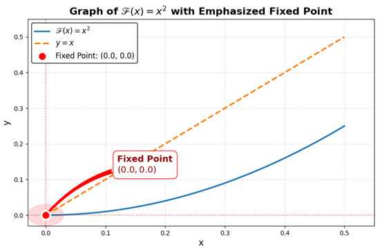
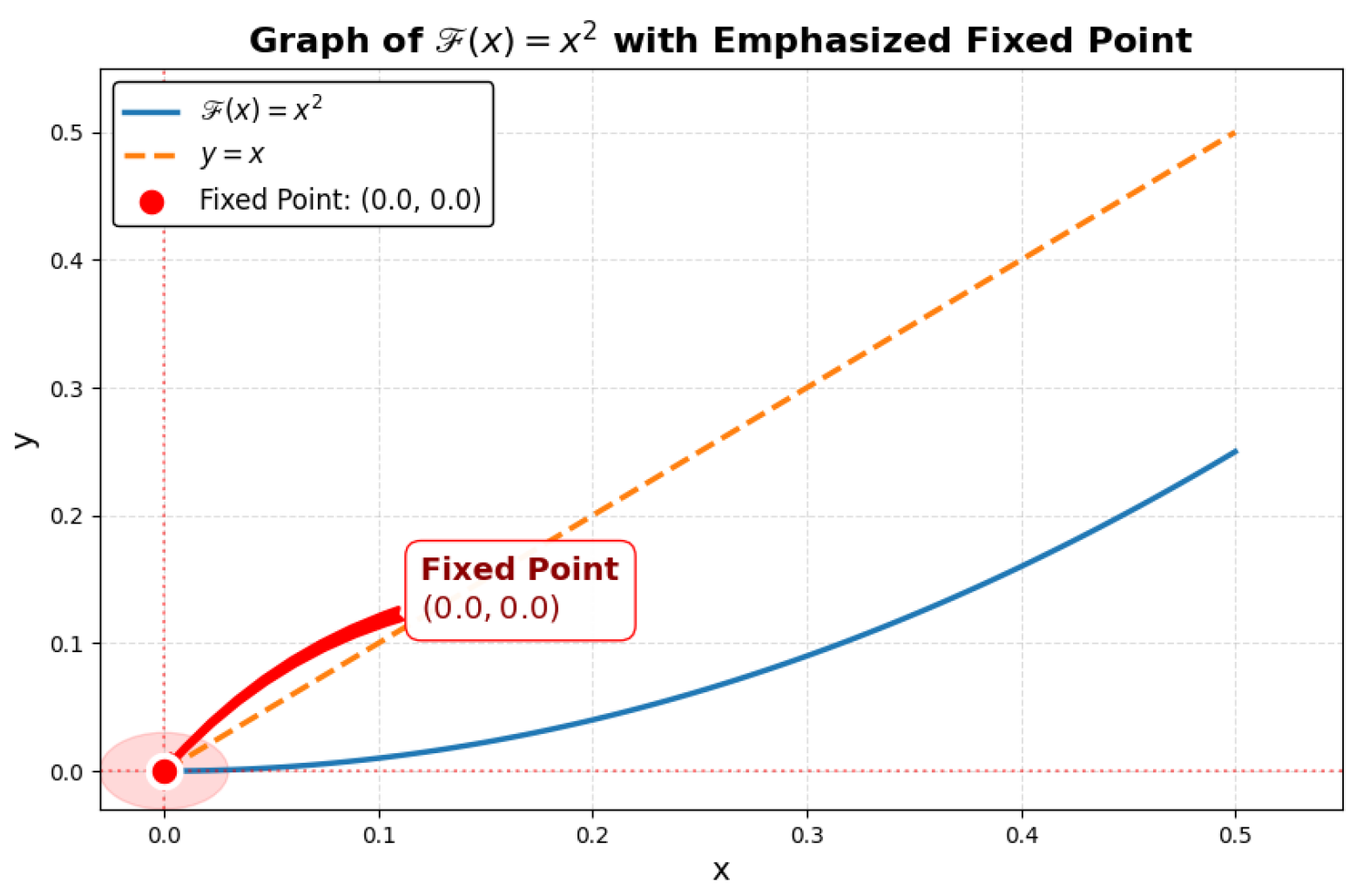
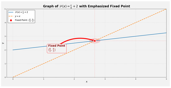
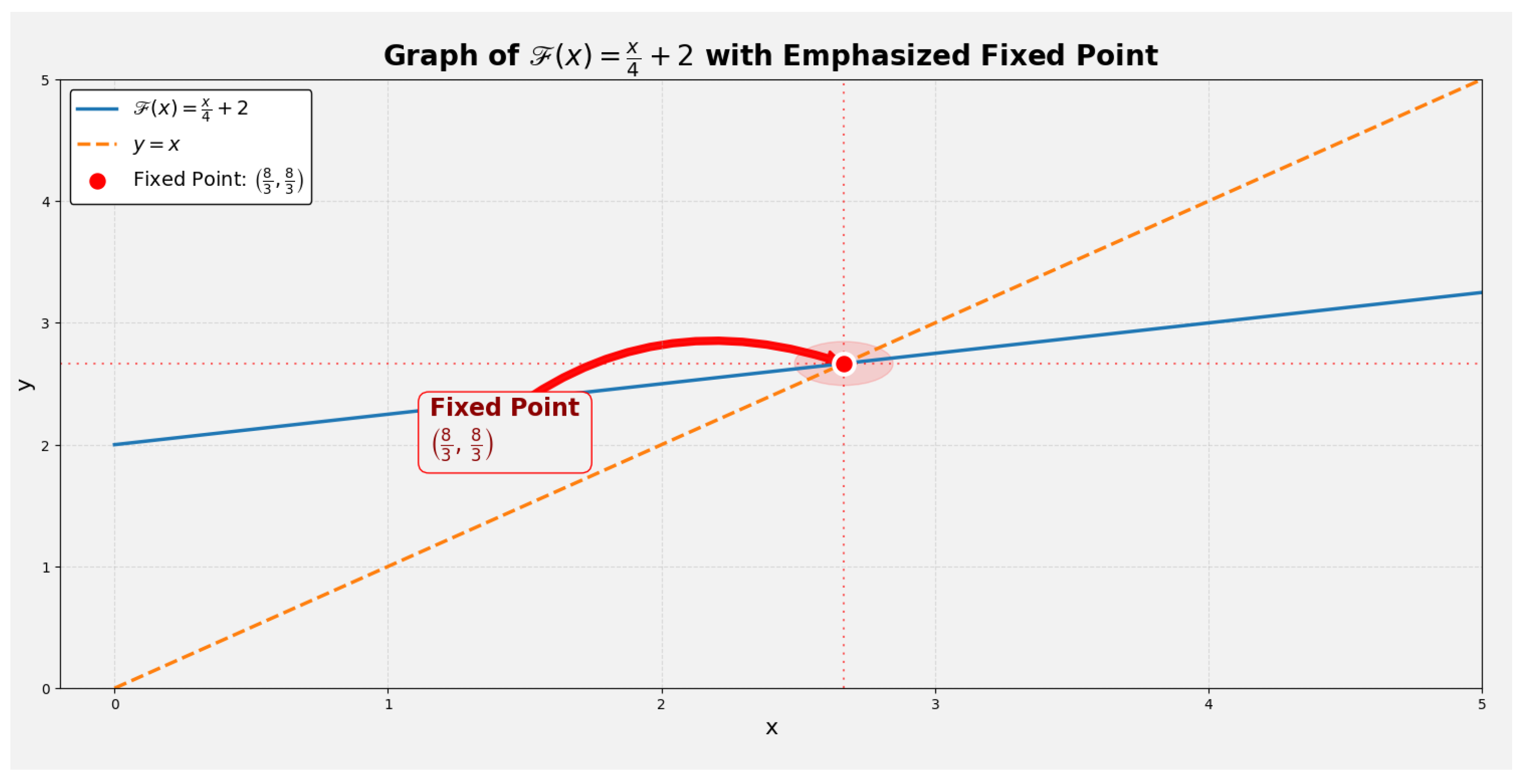
• Therefore, all the terms and conditions outlined in our main result have been met, confirming $(0,0)$ as the unique fixed point as depicted in Figure 1.
  

  Figure 1. Geometry of the fixed point of mapping $\mathfrak{Z}$ in Example 1.

Clearly Figure 1 shows $(0,0)$ is a unique fixed point for $\mathfrak{Z}=x^2$.

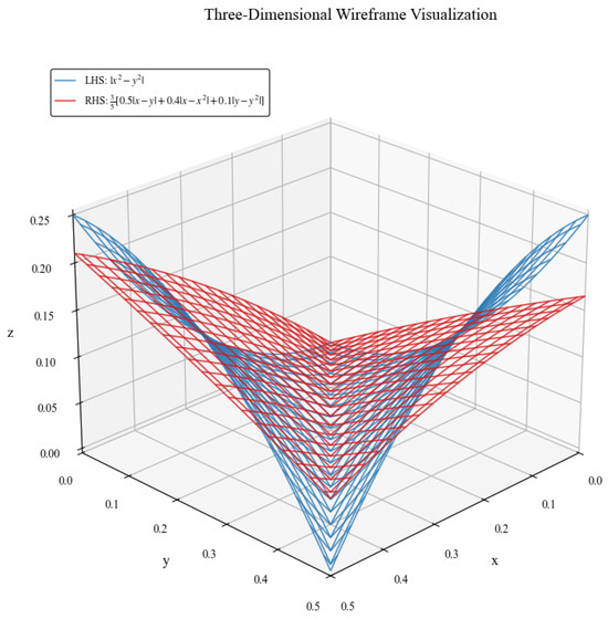
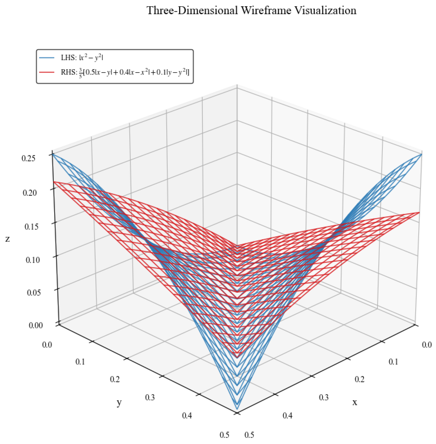
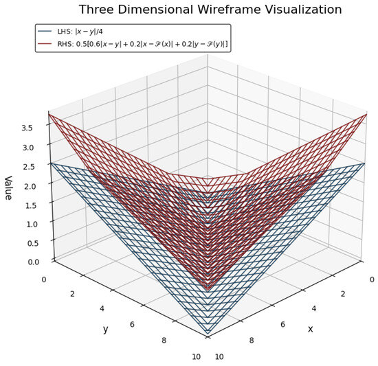
The 3D wireframe visualization of Figure 2 shows that the right-hand side of the inequality remains strictly above the left-hand side for all pairs $(x,y)$, demonstrating that the generalized contractive condition is met throughout the region. Moreover, if we take the difference of both surfaces (RHS − LHS) in Figure 2, it will be strictly positive, further confirming the validity of the inequality. These visualizations provide strong numerical and geometric evidence supporting the analytical results and ensuring the existence and uniqueness of the fixed point within the specified interval.

Figure 2. 3D wireframe visualization of the inequality in Example 1.

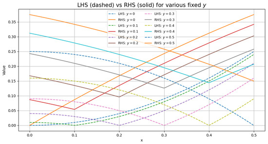
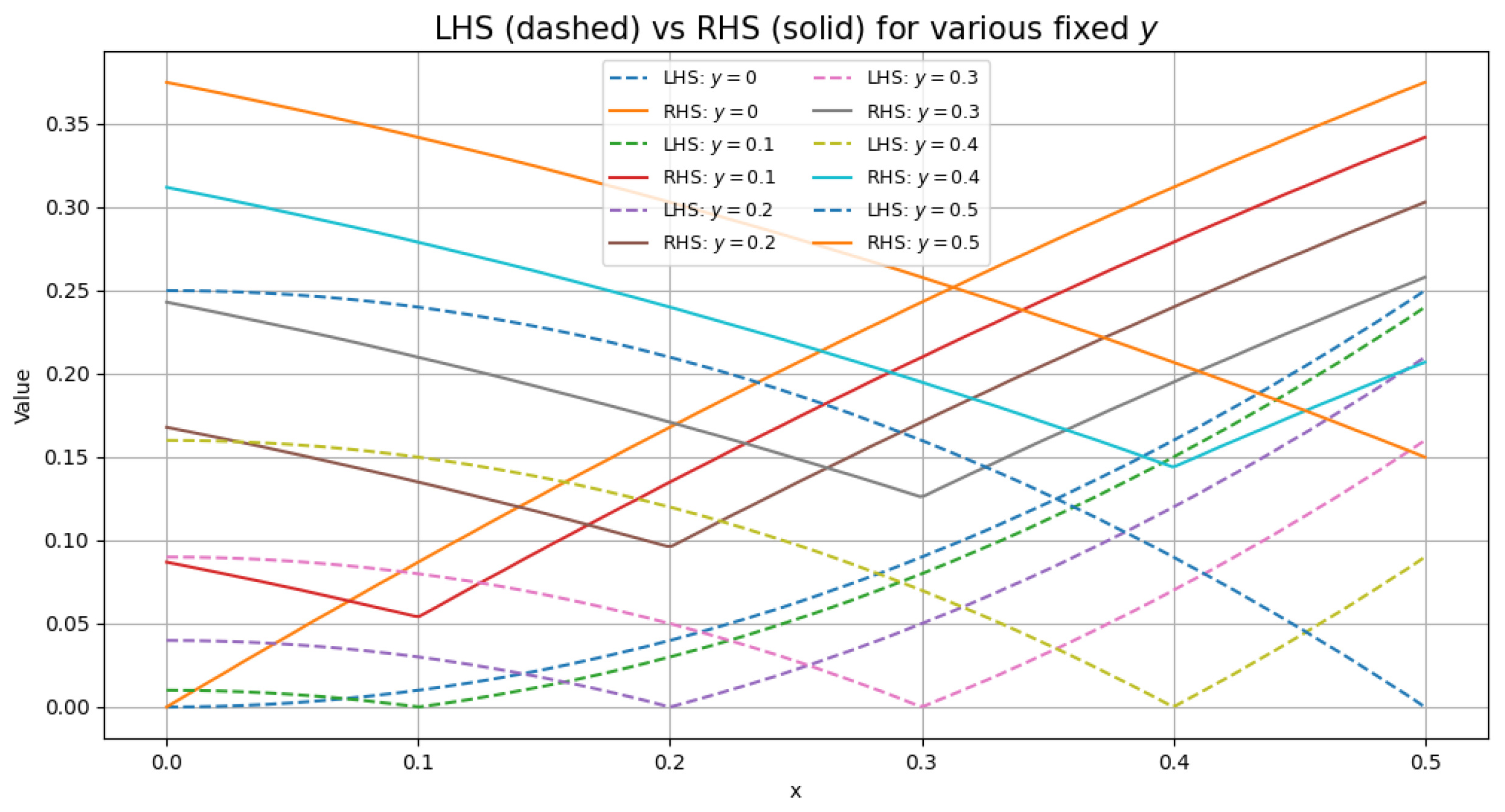
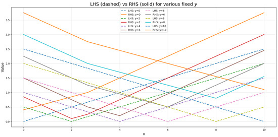
In Figure 3, the line graph shows a cross-sectional view of the contractive inequality by fixing values of y within the interval $[0,0.5]$. The dashed curve represents the expression $\mathfrak{D}(\mathfrak{Z}(x),\mathfrak{Z}(y))=|x^2-y^2|$, while the solid curve represents the right-hand side of the contractive condition. Comparing these curves directly shows that the solid curve is always above the dashed curve for all values of x, confirming that the mapping $\mathfrak{Z}(x)=x^2$ satisfies the contractive condition throughout the interval.

Figure 3. Cross-sectional view of the contractive inequality in Example 1.

Example 2. 

Let $\mathcal{A}=[0,\infty )$; with the metric defined by $\mathfrak{D}(x,y)=|x-y|$ for all $x,y\in \mathcal{A}$, $\mathcal{A}$ is a complete metric space Define

• $\mathfrak{Z}:\mathcal{A}\to \mathcal{A}$ by

$$\mathfrak{Z}(x)={\displaystyle \frac{x}{4}}+2$$

Define $F,B:[0,\infty )\to [0,\infty )$

as

$$F(\widehat{t})=\widehat{t},B(\widehat{t})=0.5\widehat{t}.$$

Clearly, $B<F$ for all $\widehat{t}>0$. As

$$\mathfrak{D}(x,y)=|x-y|,\mathfrak{D}(x,\mathfrak{Z}x)=|x-{\displaystyle \frac{x}{4}}-2|=|{\displaystyle \frac{3x}{4}}-2|,\mathfrak{D}(y,\mathfrak{Z}y)=|y-{\displaystyle \frac{y}{4}}-2|=|{\displaystyle \frac{3y}{4}}-2|$$

$$F\left(\mathfrak{D}(\mathfrak{Z}x,\mathfrak{Z}y)\right)\le B\left({\alpha }_1\mathfrak{D}(x,y)+{\alpha }_2\mathfrak{D}(x,\mathfrak{Z}x)+{\alpha }_3\mathfrak{D}(y,\mathfrak{Z}y)\right),\mathit{for}\mathit{all}x,y\in \mathcal{A}.$$

$$F\left({\displaystyle \frac{1}{4}}|x-y|\right)\le B\left({\alpha }_1|x-y|+{\alpha }_2|{\displaystyle \frac{3x}{4}}-2|+{\alpha }_3|{\displaystyle \frac{3y}{4}}-2|\right),\mathit{for}\mathit{all}x,y\in \mathcal{A}.$$

Let the constants ${\alpha }_1,{\alpha }_2,{\alpha }_3$ be given by

$${\alpha }_1=0.6,{\alpha }_2=0.2,{\alpha }_3=0.2.$$

$$F\left({\displaystyle \frac{1}{4}}|x-y|\right)\le B\left(0.6|x-y|+0.2|{\displaystyle \frac{3x}{4}}-2|+0.2|{\displaystyle \frac{3y}{4}}-2|\right),\mathit{for}\mathit{all}x,y\in \mathcal{A}.$$

Thus,

$$\left({\displaystyle \frac{1}{4}}|x-y|\right)\le 0.5\left(0.6|x-y|+0.2|{\displaystyle \frac{3x}{4}}-2|+0.2|{\displaystyle \frac{3y}{4}}-2|\right)$$

$${\displaystyle \frac{1}{4}}|x-y|\le 0.5\left(0.6|x-y|+0.2|{\displaystyle \frac{3x}{4}}-2|+0.2|{\displaystyle \frac{3y}{4}}-2|\right)$$

For all $x,y\in [0,\infty )$, one can verify (by direct algebraic manipulation or case analysis) that

$${\displaystyle \frac{1}{4}}|x-y|\le 0.5\left(0.6|x-y|+0.2|{\displaystyle \frac{3x}{4}}-2|+0.2|{\displaystyle \frac{3y}{4}}-2|\right)$$

Hence, the inequality holds, and $\mathfrak{Z}$ satisfies the given generalized contraction condition with respect to $F,B$ and ${\alpha }_1,{\alpha }_2,{\alpha }_3$.

• Therefore, all the terms and conditions outlined in our main result have been met, confirming $({\displaystyle \frac{8}{3}},{\displaystyle \frac{8}{3}})$ as the unique fixed point, as depicted in Figure 4.
  

  Figure 4. Geometry of the fixed point of mapping $\mathfrak{Z}$ in Example 2.

Clearly Figure 1 shows $({\displaystyle \frac{8}{3}},{\displaystyle \frac{8}{3}})$ is a unique fixed point for $\mathfrak{Z}={\displaystyle \frac{x}{4}}+2$.

The 3D wireframe visualization of Figure 5 shows that the right-hand side of the inequality remains strictly above the left-hand side for all pairs $(x,y)$, demonstrating that the generalized contractive condition is met throughout the region. Moreover, if we take the difference of both surfaces (RHS − LHS) in Figure 5, it will be strictly positive, further confirming the validity of the inequality. These visualizations provide strong numerical and geometric evidence supporting the analytical results and ensuring the existence and uniqueness of the fixed point within the specified interval.

Figure 5. 3D wireframe visualization of contractive condition in Example 2.

In Figure 6, the line graph shows a cross-sectional view of the contractive inequality by fixing values of y within the interval. The dashed curve represents the expression left-hand of the inequality, while the solid curve represents the right-hand side of the contractive condition. Comparing these curves directly shows that the solid curve is always above the dashed curve for all values of x, confirming that the mapping $\mathfrak{Z}(x)={\displaystyle \frac{x}{4}}+2$ satisfies the contractive condition throughout the interval.

Figure 6. Cross-sectional view of the contractive inequality in Example 2.

Remark 2. 

(1).

In $(F,B)$ contraction, if $F,B$ are defined to be identity mappings, then we recover the Reich contraction:

$$\mathfrak{D}(\mathfrak{Z}x,\mathfrak{Z}y)\le {\alpha }_1\mathfrak{D}(x,y)+{\alpha }_2\mathfrak{D}(x,\mathfrak{Z}x)+{\alpha }_3\mathfrak{D}(y,\mathfrak{Z}y)$$

$${\alpha }_1,{\alpha }_2,{\alpha }_3\in [0,1),{\alpha }_1+{\alpha }_2<1,{\alpha }_3\le 1-({\alpha }_1+{\alpha }_2).$$

(27)

(2).

Let us consider a metric space $\mathfrak{D}(x,y)=|x-y|$ and let $\mathfrak{Z}:[0,1]\to [0,1]$ be a self-mapping defined by

$$3(x)=\left\{\begin{array}{cc}{\displaystyle \frac{1}{2}},\hfill & x\in [0,{\displaystyle \frac{1}{2}}),\hfill \\ 1-x,\hfill & x\in [{\displaystyle \frac{1}{2}},1].\hfill \end{array}\right.$$

with $F(x)=xB(t)={\displaystyle \frac{1}{2}}x,$ and clearly $B(t)<F(t)$ for all $t>0.$ Let $x,y\in [{\displaystyle \frac{1}{2}},1],$ and $x={\displaystyle \frac{1}{2}},y>{\displaystyle \frac{1}{2}}.$

$$F\left(\mathfrak{D}(\mathfrak{Z}x,\mathfrak{Z}y)\right)\le B\left({\alpha }_1\mathfrak{D}(x,y)+{\alpha }_2\mathfrak{D}(x,\mathfrak{Z}x)+{\alpha }_3\mathfrak{D}(y,\mathfrak{Z}y)\right),$$

$$F\left(|1-x-1+y|\right)\le B\left({\alpha }_1|{\displaystyle \frac{1}{2}}-y|+{\alpha }_2|{\displaystyle \frac{1}{2}}-1+x|+{\alpha }_3|y-1+y|\right),$$

$$F\left(|y-{\displaystyle \frac{1}{2}}|\right)\le B\left({\alpha }_1|y-{\displaystyle \frac{1}{2}}|+{\alpha }_2|{\displaystyle \frac{1}{2}}-{\displaystyle \frac{1}{2}}|+{\alpha }_3|2y-1|\right),$$

$$|y-{\displaystyle \frac{1}{2}}|\le {\displaystyle \frac{1}{2}}\left({\alpha }_1|y-{\displaystyle \frac{1}{2}}|+{\alpha }_2\left|0\right|+{\alpha }_3|2y-1|\right).$$

Since $x,y>0,$ and $x<y$,

$$(y-{\displaystyle \frac{1}{2}})\le {\displaystyle \frac{1}{2}}\left({\alpha }_1(y-{\displaystyle \frac{1}{2}})+{\alpha }_3.2(y-{\displaystyle \frac{1}{2}})\right),$$

$$1\le {\displaystyle \frac{1}{2}}({\alpha }_1+{\alpha }_3.2).$$

Let ${\alpha }_1={\alpha }_2=0,{\alpha }_3=1,\Rightarrow {\alpha }_1+{\alpha }_2+{\alpha }_3=1$, and

$$1\le {\displaystyle \frac{1}{2}}(0+(1)(2)),$$

$$1\le 1.$$

Hence, $\mathfrak{Z}$ is an $(F,B)$-contraction. If we consider ${\alpha }_1+{\alpha }_2+{\alpha }_3<1$, then the inequality $1\le {\displaystyle \frac{1}{2}}({\alpha }_1+2{\alpha }_3)$ never holds.

It concludes that $\mathfrak{Z}$ is an (F,B)-contraction but not a Reich contraction.

(3).

If we consider ${\alpha }_2={\alpha }_3=0$, then the Reich contraction reduces to a Banach contraction.

(4).

If we consider ${\alpha }_1=0$, and let $k=max\{{\alpha }_1,{\alpha }_2\}\in (0,{\displaystyle \frac{1}{2}})$, then it becomes a Kannan Contraction.

(5).

Selecting $F(t)=\ln (t)$ and $B(t)=\ln (\lambda t)$ for $\lambda \in (0,1)$ in condition (2.5) yields the classical Ćirić–Reich–Rus contractive condition $\mathfrak{D}(\mathfrak{Z}x,\mathfrak{Z}y)\le \lambda ({\alpha }_1\mathfrak{D}(x,y)+{\alpha }_2\mathfrak{D}(x,\mathfrak{Z}x)+{\alpha }_3\mathfrak{D}(y,\mathfrak{Z}y))$, which was employed by [16] for the fractional Aizawa system. The $(F,B)$-contraction thus serves as a nonlinear extension of the linear Ćirić–Reich–Rus model. A comprehensive comparison is presented in Table 1.

Table 1. Comparison between the Ćirić–Reich–Rus approach [16] and the proposed $(F,B)$-contraction.

Feature	Ćirić-Reich-Rus Approach [16]	Proposed $(\mathit{F},\mathit{B})$-Contraction Framework
Contractive Form	$\mathfrak{D}(\mathfrak{Z}x,\mathfrak{Z}y)\le a_1\mathfrak{D}(x,y)+a_2\mathfrak{D}(x,\mathfrak{Z}x)+a_3\mathfrak{D}(y,\mathfrak{Z}y)$	$F(\mathfrak{D}(\mathfrak{Z}x,\mathfrak{Z}y))\le B({\alpha }_1\mathfrak{D}(x,y)+{\alpha }_2\mathfrak{D}(x,\mathfrak{Z}x)+{\alpha }_3\mathfrak{D}(y,\mathfrak{Z}y))$
Control Structure	Linear coefficients $a_1,a_2,a_3\ge 0$	Nonlinear auxiliary mappings $F,B:(0,\infty )\to \mathbb{R}$
Generality	Special case of $(F,B)$-contractions	Unifies Wardowski, Proinov, and Ćirić-type fixed-point results
Constraint Bounds	Strict linear bound $a_1+a_2+a_3<1$	Relaxed nonlinear control via $B(t)<F(t)$

5. Application to Fractional Aizawa Model

In this section, we analyze the fractional Aizawa system by applying the fixed-point theorem obtained in the previous section. The Aizawa system [16] contains three nonlinear differential equations and is known for its nonlinear complex chaotic dynamics. The system’s evolution is governed by the state variables $x,y,z$ alongside parameters $a,b,c,\gamma ,f$. All parameters have a specific role in creating the visualization of the model. The parameters $a,b,c,\gamma$, and f modulate the vertical stretching, symmetry, vertical displacement along the (z)-axis, rotational coupling, and chaotic behavior of the system by controlling higher-order nonlinear interactions, respectively. Understanding the behavioral bounds of the Aizawa system is crucial due to its generation of rich, multi-scroll chaotic dynamics. The recent literature has explored the use of advanced neural networks, such as time-varying fuzzy-parameter zeroing neural networks and noise-tolerant models [17,18], to govern the synchronization and stabilization of these chaotic structures. However, it is important to ensure the existence and uniqueness of solutions before implementing these control setups. This foundation is necessary for the effectiveness of the control methods.

Here the Aizawa system is selected due to its structural simplicity and rich dynamical properties, rendering it an ideal benchmark for validating both theoretical framework and numerical formulations in fractional calculus. The advanced literature reinforces the adaptability of the Aizawa system across different fields (physics, information technology, etc.), including analog and memristor-based circuit realizations [19], finding out numerical solutions for fractional systems [20], fractal and fractional chaotic dynamics [21], hybrid system architectures, and neural-network-based identification approaches [22]. The use of multiple disciplines highlights the importance of the system in nonlinear dynamics and engineering, showing that it is a strong option to showcase the practicality of the proposed results regarding existence and uniqueness.

$$\left\{\begin{array}{c}{\displaystyle \frac{dx(t)}{dt}}=(z(t)-b)x(t)-\gamma y(t)\hfill \\ {\displaystyle \frac{dy(t)}{dt}}=\gamma x(t)+(z(t)-b)y(t)\hfill \\ {\displaystyle \frac{dz(t)}{dt}}=c+az(t)-{\displaystyle \frac{z^3(t)}{3}}-(x^2(t)+y^2(t))(1+ez(t))+fz(t)x^3(t).\hfill \end{array}\right.$$

(28)

Let,

$$\left\{\begin{array}{c}{\widehat{\mathcal{E}}}_1(x(t),y(t),z(t))=(z(t)-b)x(t)-\gamma y(t),\hfill \\ {\widehat{\mathcal{E}}}_2(x(t),y(t),z(t))=\gamma x(t)+(z(t)-b)y(t),\hfill \\ {\widehat{\mathcal{E}}}_3(x(t),y(t),z(t))=c+az(t)-{\displaystyle \frac{z^3(t)}{3}}-\left(x^2(t)+y^2(t)\right)\left(1+ez(t)\right)+fz(t)x^3(t).\hfill \end{array}\right.$$

Now, we replace the classical time derivative with the fractional Atangana–Baleanu operator. The Aizawa differential system converted into Aizawa fractional system with fractional order $\tilde{\nu }\in (0,1)$. The fractional derivatives are effective mathematical tools for capturing memory and hereditary effects in a wide range of complex systems in physics, biology, and engineering. Analytical solutions for these equations are seldom feasible due to the nonlocal nature of the operators they contain, leading to a rapid development of numerical methods to solve them, creating a complete history of trajectory. The Mittag-Leffler kernel is used in the AB derivative to guarantee stability and offer a deeper insight patterns into complex dynamical systems.

$$\left\{\begin{array}{c}{}_0{}^{AB}\mathfrak{D}_t^{\tilde{\nu }}\left\{x(t)\right\}={\widehat{\mathcal{E}}}_1(x(t),y(t),z(t))\hfill \\ {}_0{}^{AB}\mathfrak{D}_t^{\tilde{\nu }}\left\{y(t)\right\}={\widehat{\mathcal{E}}}_2(x(t),y(t),z(t))\hfill \\ {}_0{}^{AB}\mathfrak{D}_t^{\tilde{\nu }}\left\{z(t)\right\}={\widehat{\mathcal{E}}}_3(x(t),y(t),z(t))\hfill \end{array}\right.$$

(29)

The AB-derivative definition enables the system to be expressed as a fractional Volterra integral equation through a specific process.

$$\begin{array}{c}\hfill \left\{\begin{array}{cc}x(t)-{\widehat{\tilde{\upsilon }}}_1(t)\hfill & ={\displaystyle \frac{1-\tilde{\nu }}{\widehat{\mathcal{C}}(\tilde{\nu })}}{\widehat{\mathcal{E}}}_1(x(t),y(t),z(t))+{\displaystyle \frac{\tilde{\nu }}{\widehat{\mathcal{C}}(\tilde{\nu })\Gamma (\tilde{\nu })}}{\int }_0^t{(t-\widehat{r})}^{\tilde{\nu }-1}{\widehat{\mathcal{E}}}_1(x(\widehat{r}),y(\widehat{r}),z(\widehat{r}))d\widehat{r}\hfill \\ y(t)-{\widehat{\tilde{\upsilon }}}_2(t)\hfill & ={\displaystyle \frac{1-\tilde{\nu }}{\widehat{\mathcal{C}}(\tilde{\nu })}}{\widehat{\mathcal{E}}}_2(x(t),y(t),z(t))+{\displaystyle \frac{\tilde{\nu }}{\widehat{\mathcal{C}}(\tilde{\nu })\Gamma (\tilde{\nu })}}{\int }_0^t{(t-\widehat{r})}^{\tilde{\nu }-1}{\widehat{\mathcal{E}}}_2(x(\widehat{r}),y(\widehat{r}),z(\widehat{r}))d\widehat{r}\hfill \\ z(t)-{\widehat{\tilde{\upsilon }}}_3(t)\hfill & ={\displaystyle \frac{1-\tilde{\nu }}{\widehat{\mathcal{C}}(\tilde{\nu })}}{\widehat{\mathcal{E}}}_3(x(t),y(t),z(t))+{\displaystyle \frac{\tilde{\nu }}{\widehat{\mathcal{C}}(\tilde{\nu })\Gamma (\tilde{\nu })}}{\int }_0^t{(t-\widehat{r})}^{\tilde{\nu }-1}{\widehat{\mathcal{E}}}_3(x(\widehat{r}),y(\widehat{r}),z(\widehat{r}))d\widehat{r}.\hfill \end{array}\right.\end{array}$$

(30)

The previously described iterative methodology is now demonstrated in the following list:

$$x(0)={\widehat{\tilde{\upsilon }}}_1(t),y(0)={\widehat{\tilde{\upsilon }}}_2(t),z(0)={\widehat{\tilde{\upsilon }}}_3(t).$$

Afterward, the system in Equation (30) is altered to

$$\begin{array}{c}\hfill \left\{\begin{array}{cc}x(t)\hfill & =x(0)+{\displaystyle \frac{1-\tilde{\nu }}{\widehat{\mathcal{C}}(\tilde{\nu })}}{\widehat{\mathcal{E}}}_1(x(t),y(t),z(t))+{\displaystyle \frac{\tilde{\nu }}{\widehat{\mathcal{C}}(\tilde{\nu })\Gamma (\tilde{\nu })}}{\int }_0^t{(t-\widehat{r})}^{\tilde{\nu }-1}{\widehat{\mathcal{E}}}_1(x(\widehat{r}),y(\widehat{r}),z(\widehat{r}))d\widehat{r}\hfill \\ y(t)\hfill & =y(0)+{\displaystyle \frac{1-\tilde{\nu }}{\widehat{\mathcal{C}}(\tilde{\nu })}}{\widehat{\mathcal{E}}}_2(x(t),y(t),z(t))+{\displaystyle \frac{\tilde{\nu }}{\widehat{\mathcal{C}}(\tilde{\nu })\Gamma (\tilde{\nu })}}{\int }_0^t{(t-\widehat{r})}^{\tilde{\nu }-1}{\widehat{\mathcal{E}}}_2(x(\widehat{r}),y(\widehat{r}),z(\widehat{r}))d\widehat{r}\hfill \\ z(t)\hfill & =z(0)+{\displaystyle \frac{1-\tilde{\nu }}{\widehat{\mathcal{C}}(\tilde{\nu })}}{\widehat{\mathcal{E}}}_3(x(t),y(t),z(t))+{\displaystyle \frac{\tilde{\nu }}{\widehat{\mathcal{C}}(\tilde{\nu })\Gamma (\tilde{\nu })}}{\int }_0^t{(t-\widehat{r})}^{\tilde{\nu }-1}{\widehat{\mathcal{E}}}_3(x(\widehat{r}),y(\widehat{r}),z(\widehat{r}))d\widehat{r},\hfill \end{array}\right.\end{array}$$

(31)

that yields the recursion expressions

$$\begin{array}{c}\hfill \left\{\begin{array}{cc}{x}_n(t)\hfill & ={\displaystyle \frac{1-\tilde{\nu }}{\widehat{\mathcal{C}}(\tilde{\nu })}}{\widehat{\mathcal{E}}}_1(x_{n-1}(t),y_{n-1}(t),z_{n-1}(t))+{\displaystyle \frac{\tilde{\nu }}{\widehat{\mathcal{C}}(\tilde{\nu })\Gamma (\tilde{\nu })}}{\int }_0^t{(t-\widehat{r})}^{\tilde{\nu }-1}{\widehat{\mathcal{E}}}_1(x_{n-1}(\widehat{r}),y_{n-1}(\widehat{r}),z_{n-1}(\widehat{r}))d\widehat{r}\hfill \\ y_n(t)\hfill & ={\displaystyle \frac{1-\tilde{\nu }}{\widehat{\mathcal{C}}(\tilde{\nu })}}{\widehat{\mathcal{E}}}_2(x_{n-1}(t),y_{n-1}(t),z_{n-1}(t))+{\displaystyle \frac{\tilde{\nu }}{\widehat{\mathcal{C}}(\tilde{\nu })\Gamma (\tilde{\nu })}}{\int }_0^t{(t-\widehat{r})}^{\tilde{\nu }-1}{\widehat{\mathcal{E}}}_2(x_{n-1}(\widehat{r}),y_{n-1}(\widehat{r}),z_{n-1}(\widehat{r})d\widehat{r}\hfill \\ z_n(t)\hfill & ={\displaystyle \frac{1-\tilde{\nu }}{\widehat{\mathcal{C}}(\tilde{\nu })}}{\widehat{\mathcal{E}}}_3(x_{n-1}(t),y_{n-1}(t),z_{n-1}(t))+{\displaystyle \frac{\tilde{\nu }}{\widehat{\mathcal{C}}(\tilde{\nu })\Gamma (\tilde{\nu })}}{\int }_0^t{(t-\widehat{r})}^{\tilde{\nu }-1}{\widehat{\mathcal{E}}}_3(x_{n-1}(\widehat{r}),y_{n-1}(\widehat{r}),z_{n-1}(\widehat{r}))d\widehat{r}.\hfill \end{array}\right.\end{array}$$

(32)

Now we state the main application theorem for the existence and uniqueness of solutions for the fractional Azawa system. It is remarked that the specific parameters of the fractional Azawa model are chosen to meet the contractive condition outlined in Theorem 6; the fixed-point results from the previous section can be used to ensure the existence and uniqueness of the solution. More explicitly, when the parameter sets meet the necessary contractive condition, the iterative scheme will converge to the unique fixed point. On the other hand, parameter choices that do not satisfy the contractive condition such as standard parameters, are not accounted for by the fixed-point theorem and may display non-convergent or chaotic dynamics.

Theorem 6. 

Let $\mathcal{A}=C([0,t_{\max }],{\mathbb{R}}^3)$ and $\mathfrak{Z}:\mathcal{A}\to \mathcal{A}$ be associated with the fractional Aizawa system under the Atangana–Baleanu derivative of order $\tilde{\nu }\in (0,1)$. If the following conditions hold,

(i)

Boundedness condition:

$${\displaystyle \frac{\Gamma (\tilde{\nu })(1-\tilde{\nu })+t^{\tilde{\nu }}}{\mathcal{C}(\tilde{\nu })\Gamma (\tilde{\nu })}}\le {\displaystyle \frac{1}{2}},$$

(ii)

Contractive condition:

$$\begin{array}{cc}& \mathrm{For}\mathrm{any},U_1=((x_1(t),y_1(t),z_1(t))),U_2=(x_2(t),y_2(t),z_2(t))\in \mathcal{A}.\hfill \\ & \left|{\widehat{\mathcal{E}}}_1(U_1(t))-{\widehat{\mathcal{E}}}_1(U_2(t))\right|\le {\alpha }_1\left|U_1(t)-U_2(t)\right|+{\alpha }_2\left|U_1(t)-\mathfrak{Z}{U}_1(t)\right|+{\alpha }_3\left|U_2(t)-\mathfrak{Z}{U}_2(t)\right|\hfill \end{array}$$

with ${\alpha }_1,{\alpha }_2\in [0,1)$, ${\alpha }_1+{\alpha }_2<1$ and ${\alpha }_3\le 1-{\alpha }_1-{\alpha }_2$

then the operator $\mathfrak{Z}$ admits a unique fixed point in $\mathcal{A}$. Consequently, the fractional Aizawa system with an Atangana–Baleanu derivative possesses a unique solution on $[0,t_{\max }]$.

Proof. 

Let $\mathcal{A}=C([0,t_{\max }],{\mathbb{R}}^3)$ be a space of all continuous functions defined on $[0,t_{\max }]$, and define the functional $\mathfrak{D}:\mathcal{A}\times \mathcal{A}\to [0,\infty )$ by

$$\mathfrak{D}\left(U_1(t),U_2(t))\right)=\underset{t\in [0,t_{\max }]}{\sup }|U_1(t)-U_2(t)|$$

Then $(\mathcal{A},\mathfrak{D})$ is a complete metric space. We know that the fractional Aizawa system can be expressed in integral form via the Atangana–Baleanu derivative:

$$\begin{array}{c}\hfill \left\{\begin{array}{cc}\mathfrak{Z}(U(t))\hfill & {\displaystyle =U(0)+{\displaystyle \frac{1-\tilde{\nu }}{\widehat{\mathcal{C}}(\tilde{\nu })}}{\widehat{\mathcal{E}}}_1(U(t))+{\displaystyle \frac{\tilde{\nu }}{\widehat{\mathcal{C}}(\tilde{\nu })\Gamma (\tilde{\nu })}}{\int }_0^t{(t-\widehat{r})}^{\tilde{\nu }-1}{\widehat{\mathcal{E}}}_1(U(\widehat{r}))d\widehat{r},}\hfill \\ \mathfrak{Z}(U(t))\hfill & {\displaystyle =U(0)+{\displaystyle \frac{1-\tilde{\nu }}{\widehat{\mathcal{C}}(\tilde{\nu })}}{\widehat{\mathcal{E}}}_2(U(t))+{\displaystyle \frac{\tilde{\nu }}{\widehat{\mathcal{C}}(\tilde{\nu })\Gamma (\tilde{\nu })}}{\int }_0^t{(t-\widehat{r})}^{\tilde{\nu }-1}{\widehat{\mathcal{E}}}_2(U(\widehat{r}))d\widehat{r},}\hfill \\ \mathfrak{Z}(U(t))\hfill & {\displaystyle =U(0)+{\displaystyle \frac{1-\tilde{\nu }}{\widehat{\mathcal{C}}(\tilde{\nu })}}{\widehat{\mathcal{E}}}_3(U(t))+{\displaystyle \frac{\tilde{\nu }}{\widehat{\mathcal{C}}(\tilde{\nu })\Gamma (\tilde{\nu })}}{\int }_0^t{(t-\widehat{r})}^{\tilde{\nu }-1}{\widehat{\mathcal{E}}}_3(U(\widehat{r}))d\widehat{r}.}\hfill \end{array}\right.\end{array}$$

(33)

It is obvious that ${\widehat{r}}_i$ is continuous, so $\mathfrak{Z}$ maps continuous functions to continuous functions. Thus, $\mathfrak{Z}:\mathcal{A}\to \mathcal{A}$ is well defined. Moreover, for finite $t_{\max }$, the integral term is bounded by ${\displaystyle \frac{t^{\tilde{\nu }}}{\tilde{\nu }}}$. Hence, $\mathfrak{Z}x,\mathfrak{Z}y,\mathfrak{Z}z$ remain continuous and bounded on $[0,t_{\max }]$. Therefore, $\mathfrak{Z}(\mathcal{A})\subseteq \mathcal{A}$.

Now, we establish the existence and uniqueness of system (33) by applying our fixed-point theorem along with the assumptions (i) and (ii). We consider

$$\begin{array}{cc}& \left|\mathfrak{Z}{U}_1(t)-\mathfrak{Z}{U}_2(t)\right|\hfill \\ & =\left|\left({\displaystyle \frac{1-\tilde{\nu }}{\mathcal{C}(\tilde{\nu })}}\right)\left\{{\widehat{\mathcal{E}}}_1(U_1(t))-{\widehat{\mathcal{E}}}_1(U_2(t))\right\}\right.\hfill \\ & \left.+{\displaystyle \frac{\tilde{\nu }}{\mathcal{C}(\tilde{\nu })\tilde{\Gamma }(\tilde{\nu })}}{\int }_0^t{(t-\widehat{r})}^{\tilde{\nu }-1}\left\{{\widehat{\mathcal{E}}}_1(U_1(\widehat{r}))-{\widehat{\mathcal{E}}}_2(U_2(\widehat{r}))\right\}d\widehat{r}\right|\hfill \\ & \le \left({\displaystyle \frac{1-\tilde{\nu }}{\mathcal{C}(\tilde{\nu })}}\right)\left|{\widehat{\mathcal{E}}}_1(U_1(\widehat{r}))-{\widehat{\mathcal{E}}}_1(U_2(\widehat{r}))\right|\hfill \\ & +\left({\displaystyle \frac{\tilde{\nu }}{\mathcal{C}(\tilde{\nu })\tilde{\Gamma }(\tilde{\nu })}}\right)\left|{\widehat{\mathcal{E}}}_1(U_1(\widehat{r}))-{\widehat{\mathcal{E}}}_1(U_2(\widehat{r}))\right|\left({\displaystyle \frac{t^{\tilde{\nu }}}{\tilde{\nu }}}\right)\hfill \\ & \le \left({\displaystyle \frac{1-\tilde{\nu }}{\mathcal{C}(\tilde{\nu })}}\right)\left|{\widehat{\mathcal{E}}}_1(U_1(t))-{\widehat{\mathcal{E}}}_1(U_2(t))\right|\hfill \\ & +\left({\displaystyle \frac{\tilde{\nu }}{\mathcal{C}(\tilde{\nu })\tilde{\Gamma }(\tilde{\nu })}}\right)\left|{\widehat{\mathcal{E}}}_1(U_1(t))-{\widehat{\mathcal{E}}}_1(U_2(t))\right|\left({\displaystyle \frac{t^{\tilde{\nu }}}{\tilde{\nu }}}\right)\hfill \end{array}$$

$$\begin{array}{cc}& \le \left[\left({\displaystyle \frac{1-\tilde{\nu }}{\mathcal{C}(\tilde{\nu })}}\right)+\left({\displaystyle \frac{t^{\tilde{\nu }}}{\mathcal{C}(\tilde{\nu })\tilde{\Gamma }(\tilde{\nu })}}\right)\right]\left|{\widehat{\mathcal{E}}}_1(U_1(t))-{\widehat{\mathcal{E}}}_1(U_2(t))\right|\hfill \\ & \le \left({\alpha }_1\left|U_1(t)-U_2(t)\right|+{\alpha }_2\left|U_1(t)-\mathfrak{Z}{U}_1(t)\right|\right.\times \left({\displaystyle \frac{t^{\tilde{\nu }}+\tilde{\Gamma }(\tilde{\nu })(1-\tilde{\nu })}{\mathcal{C}(\tilde{\nu })\tilde{\Gamma }(\tilde{\nu })}}\right)\hfill \\ & \le 0.5\left({\alpha }_1\left|U_1(t)-U_2(t)\right|+{\alpha }_2\left|U_1(t)-\mathfrak{Z}{U}_1(t)\right|\right.\hfill \\ & \left.+{\alpha }_3\left|U_2(t)-\mathfrak{Z}{U}_2(t)\right|\right).\hfill \end{array}$$

Since $t\in [0,t_{\max }]$,

$$\underset{t\in [0,t_{\max }]}{\sup }|U_1(t)-U_2(t)|\le 0.5\left({\alpha }_1\underset{t\in [0,t_{\max }]}{\sup }\left|U_1(t)-U_2(t)\right|+{\alpha }_2\underset{t\in [0,t_{\max }]}{\sup }\left|U_1(t)-\mathfrak{Z}{U}_1(t)\right|+{\alpha }_3\underset{t\in [0,t_{\max }]}{\sup }\left|U_2(t)-\mathfrak{Z}{U}_2(t)\right|\right)$$

Based on the previously established inequality, we conclude the following:

$$\begin{array}{cc}\hfill \mathfrak{D}\left(\mathfrak{Z}{U}_1(t),\mathfrak{Z}{U}_2(t)\right)& \le 0.5({\alpha }_1\mathfrak{D}\left(U_1(t),U_2(t)\right)\hfill \\ & +{\alpha }_2\mathfrak{D}\left(U_1(t),\mathfrak{Z}{U}_1(t)\right)\hfill \\ & +{\alpha }_3\mathfrak{D}\left(U_2(t),\mathfrak{Z}{U}_2(t)\right)).\hfill \end{array}$$

Hence, by meeting all the outlined requirements in the main result, a unique solution for the system is guaranteed. □

Remark 3. 

Condition (i) in Theorem 6 defines a local time horizon $T_0$ for which existence and uniqueness are guaranteed. For instance, using $\tilde{\nu }=0.995$ and $\mathcal{C}(\tilde{\nu })=1$, condition (i) gives $T_0\approx 0.495$. On $[0,T_0]$, the operator $\mathfrak{Z}$ is a strict contraction. Beyond $T_0$, the contraction condition may be violated, allowing complex, non-convergent, and chaotic dynamics to arise over larger time horizons.

6. Stability Analysis of the Aizawa Attractor Fixed Points

In this section, we will be examining the conditions necessary for a stable fixed point. Equilibrium points occur when all time fractional derivatives are zero. To determine stability in the fractional Aizawa system, we will create the Jacobian matrix at equilibrium points and calculate the eigenvalues of this matrix. If the real parts of these eigenvalues are negative, then the fixed point is considered stable.

• Let $(x^{\ast },y^{\ast },z^{\ast }(t))$ be the equilibrium point for an Azawa fractional system. It is known that an equilibrium point satisfies the following equations:

  $${}_0{}^{AB}\mathfrak{D}_t^{\tilde{\nu }}\left\{x(t)\right\}=0,{}_0{}^{AB}\mathfrak{D}_t^{\tilde{\nu }}\left\{y(t)\right\}=0,{}_0{}^{AB}\mathfrak{D}_t^{\tilde{\nu }}\left\{z(t)\right\}=0.$$

  From the first two equations, we have

  $$(z(t)-b)x(t)-\gamma y(t)=0.$$

  $$\gamma x(t)+(z(t)-b)y(t)=0.$$

If $x(t)\ne 0$ and $y(t)\ne 0$ for all t, then $y(t)={\displaystyle \frac{(z(t)-b)x(t)}{\gamma }}$. Substituting this expression into the second equation gives

$$\gamma x(t)+{\displaystyle \frac{{(z(t)-b)}^{2}x(t)}{\gamma }}=0\Rightarrow x(t)\left({\gamma }^2+{(z(t)-b)}^2\right)=0$$

Since $\gamma \ne 0$ and we assumed $x(t)\ne 0$, the term $\left({\gamma }^2+{(z(t)-b)}^2\right)$ cannot equal zero for any real coordinates. Thus, no real off-axis fixed points exist. The system possesses equilibrium points localized strictly on the z-axis where

$$x^{\ast }=0,y^{\ast }=0$$

Substituting $x^{\ast }=0$ and $y^{\ast }=0,z(t)=z^{\ast }(t)$ into the third fractional differential equation,

$${}_0{}^{AB}\mathfrak{D}_t^{\tilde{\nu }}\left\{z(t)\right\}=0.$$

$$\Rightarrow c+a{z}^{\ast }(t)-{\displaystyle \frac{{(z^{\ast }(t))}^3}{3}}=0$$

Any real root $z^{\ast }(t)$ solving this cubic polynomial defines a valid system equilibrium point at $(0,0,z^{\ast }(t))$.

6.1. Constructing the Jacobian Matrix

To determine the stability of the system at $(0,0,z^{\ast }(t))$, we compute the Jacobian matrix J of partial derivatives. Let

$${}_0{}^{AB}\mathfrak{D}_t^{\tilde{\nu }}\left\{x(t)\right\}=\dot{x}(t),{}_0{}^{AB}\mathfrak{D}_t^{\tilde{\nu }}\left\{y(t)\right\}=\dot{y}(t),\mathrm{and} {}_0{}^{AB}\mathfrak{D}_t^{\tilde{\nu }}\left\{z(t)\right\}=\dot{z}(t).$$

$$J=\left(\begin{array}{ccc}{\displaystyle \frac{\partial \dot{x}(t)}{\partial x(t)}}& {\displaystyle \frac{\partial \dot{x}(t)}{\partial y(t)}}& {\displaystyle \frac{\partial \dot{x}(t)}{\partial z(t)}}\\ {\displaystyle \frac{\partial \dot{y}(t)}{\partial x(t)}}& {\displaystyle \frac{\partial \dot{y}(t)}{\partial y(t)}}& {\displaystyle \frac{\partial \dot{y}(t)}{\partial z(t)}}\\ {\displaystyle \frac{\partial \dot{z}(t)}{\partial x(t)}}& {\displaystyle \frac{\partial \dot{z}(t)}{\partial y(t)}}& {\displaystyle \frac{\partial \dot{z}(t)}{\partial z(t)}}\end{array}\right)$$

Evaluating the algebraic partial derivatives explicitly at the localized coordinate point $(0,0,z^{\ast }(t))$ simplifies the matrix layout:

$$J_{(0,0,z^{\ast }(t))}=\left(\begin{array}{ccc}{z}^{\ast }(t)-b& -\gamma & 0\\ \gamma & z^{\ast }(t)-b& 0\\ 0& 0& a-{(z^{\ast }(t))}^2\end{array}\right)$$

6.2. Deriving Eigenvalues and Stability Constraints

The characteristic eigenvalues ($\mu$) are computed by solving the determinant equation $|J-\mu I|=O$:

$$\left|\begin{array}{ccc}{z}^{\ast }(t)-b-\lambda & -\gamma & 0\\ \gamma & z^{\ast }(t)-b-\lambda & 0\\ 0& 0& a-{(z^{\ast }(t))}^2-\lambda \end{array}\right|=O$$

Using the property of the triangular matrix and exploiting the zero entries occupying the third row and column allows direct factorization into the following:

$$\left({(z^{\ast }(t)-b-\lambda )}^2+{\gamma }^2\right)·\left(a-{(z^{\ast }(t))}^2-\lambda \right)=0$$

This equation yields three distinct system eigenvalues:

$${\mu }_1=a-{(z^{\ast }(t))}^2$$

$${\mu }_2,{\mu }_3=(z^{\ast }(t)-b)\pm i\gamma$$

According to the Routh–Hurwitz criteria and linear stability theory, a fixed point is asymptotically stable if and only if the real components of all eigenvalues are strictly negative ($\mathrm{Re}({\mu }_i)<0$):

• From ${\mu }_1$: We require $a-{(z^{\ast }(t))}^2<0,\Rightarrow {(z^{\ast }(t))}^2>a$.
• From ${\mu }_{2,3}$: We require $\mathrm{Re}((z^{\ast }(t)-b)\pm i\gamma )<0\Rightarrow z^{\ast }(t)<b$.

If we solve $c+a{z}^{\ast }(t)-{\displaystyle \frac{{(z^{\ast }(t))}^3}{3}}=0$ substituting fixed parameters $(a,b,c)=(0.95,0.70,0.60)$, we get real roots

$$z_1^{\ast }\approx 1.9367,z_2^{\ast }\approx -0.8038,z_3^{\ast }\approx -1.1328$$

Clearly, $z_1^{\ast }$ violates condition $z^{\ast }(t)<b$ and $z_1^{\ast }$ condition ${(z^{\ast }(t))}^2>a$. They both are unstable points, while $z_3^{\ast }$ satisfies both conditions, so it is consider a stable points for selected parameters. This yields three real roots.

7. Numerical Results for Fractional Models

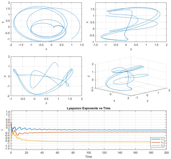
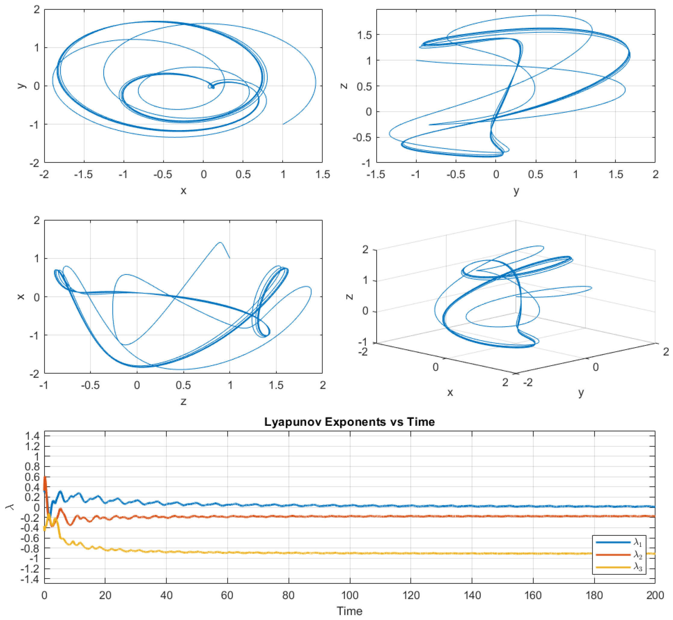
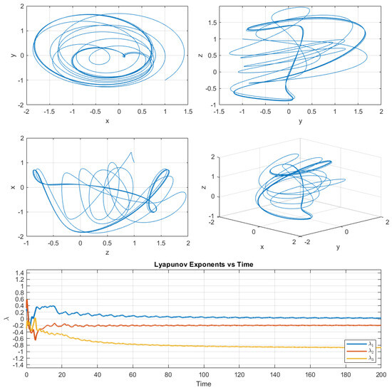
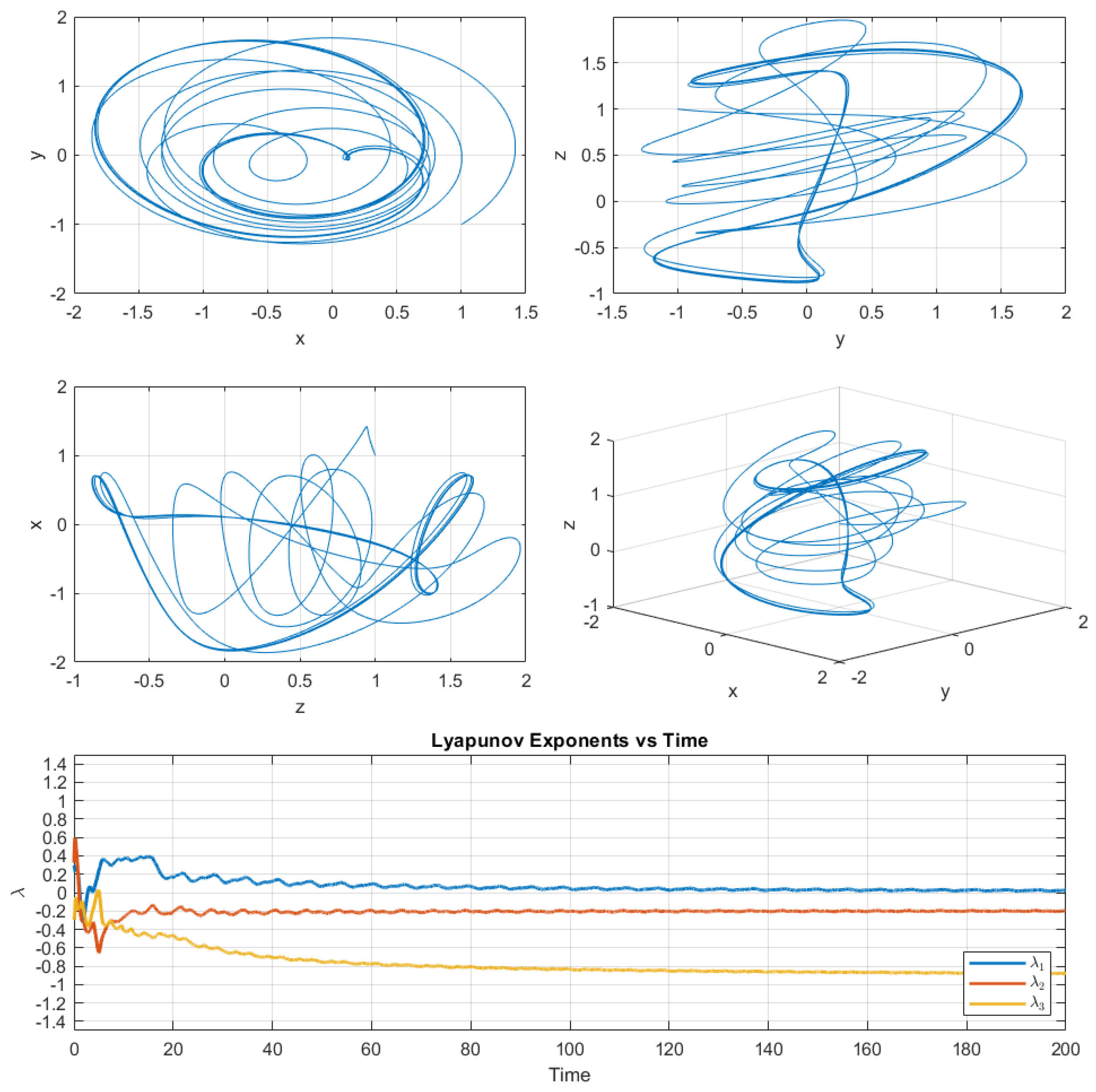
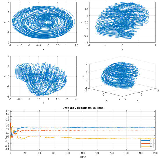
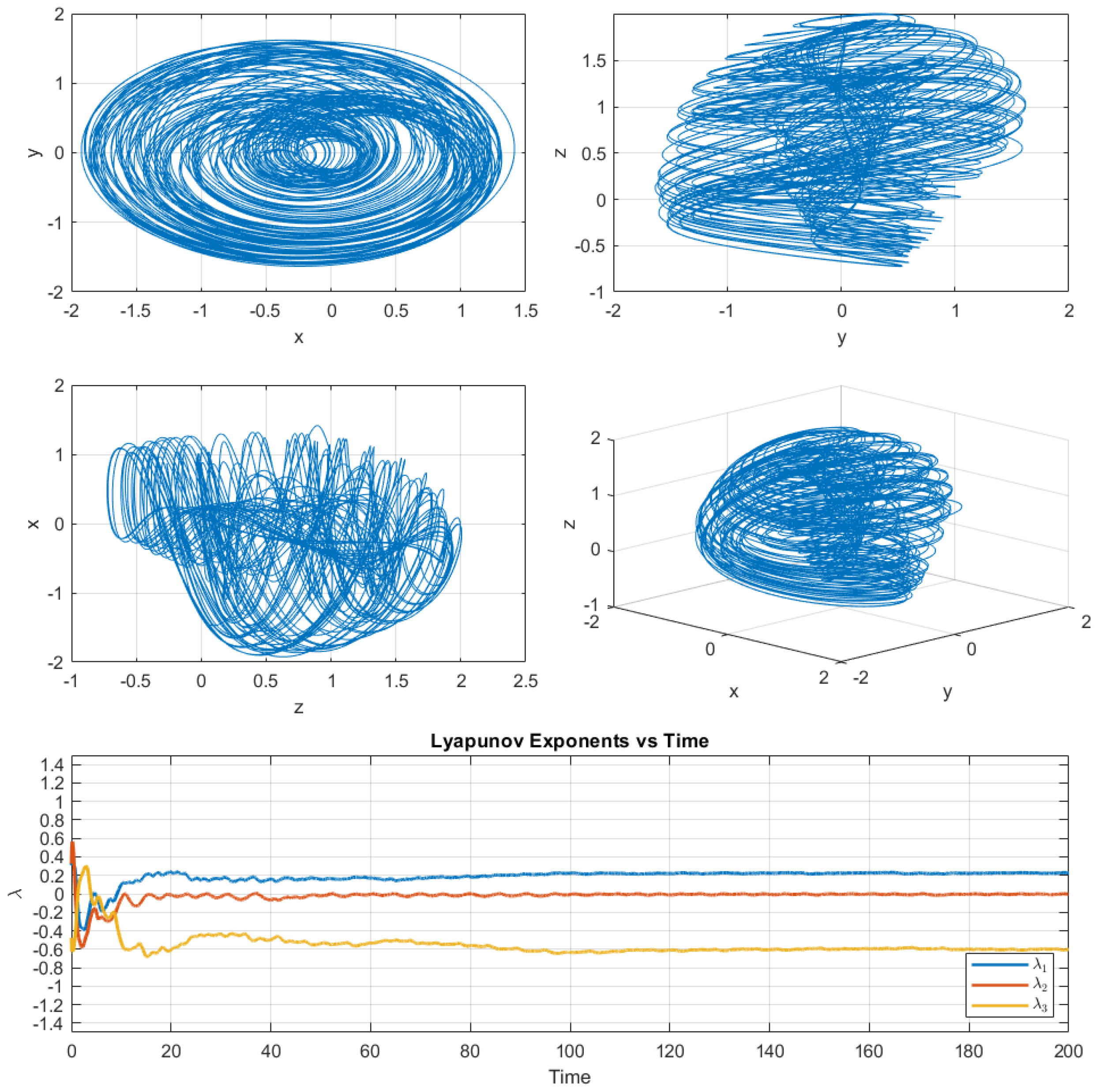
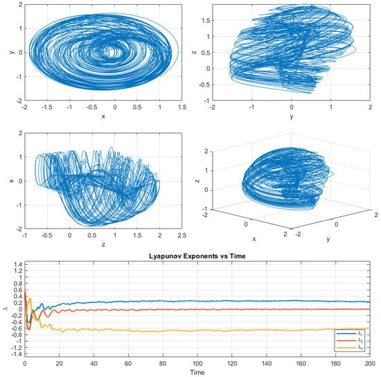
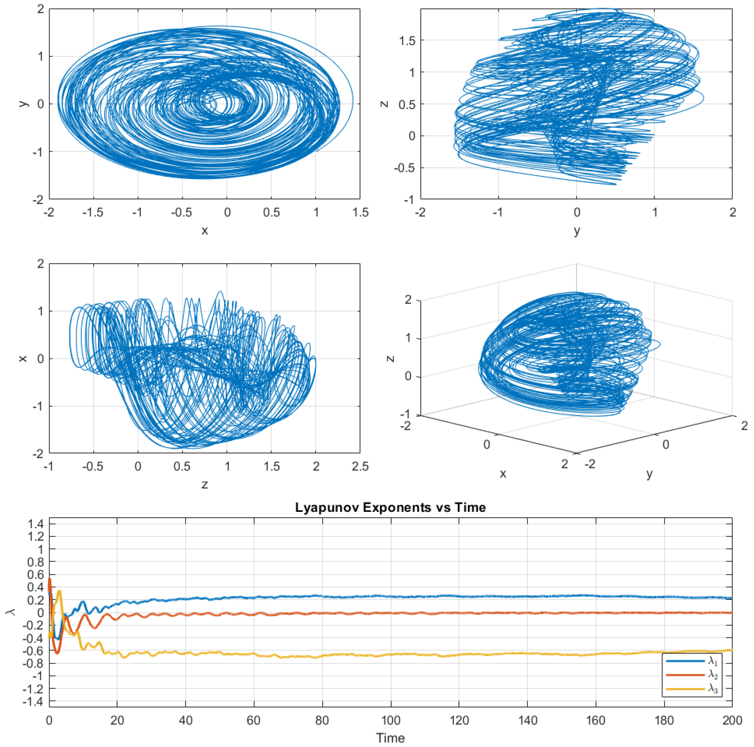
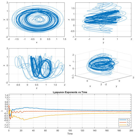
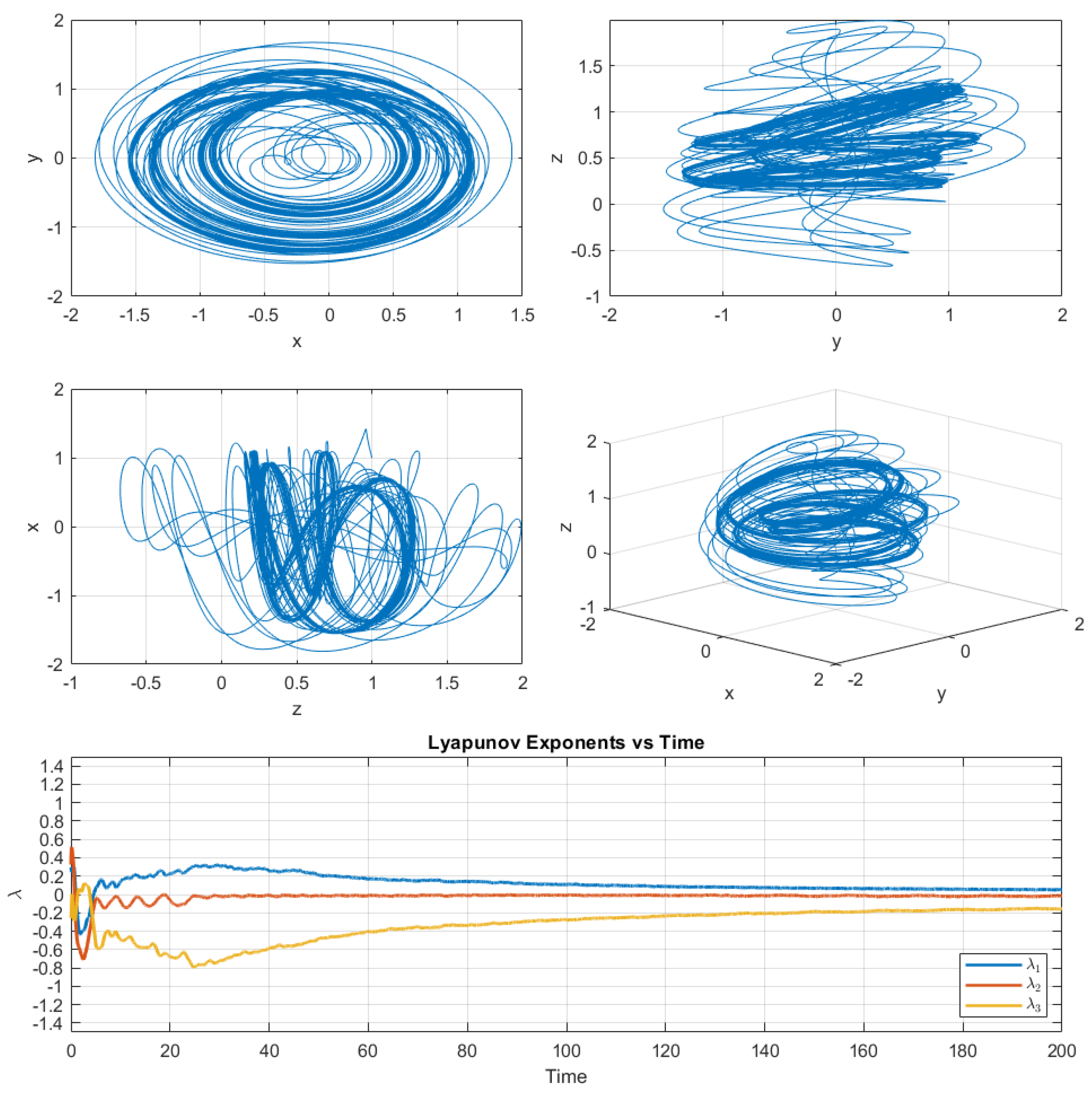
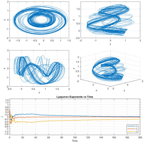
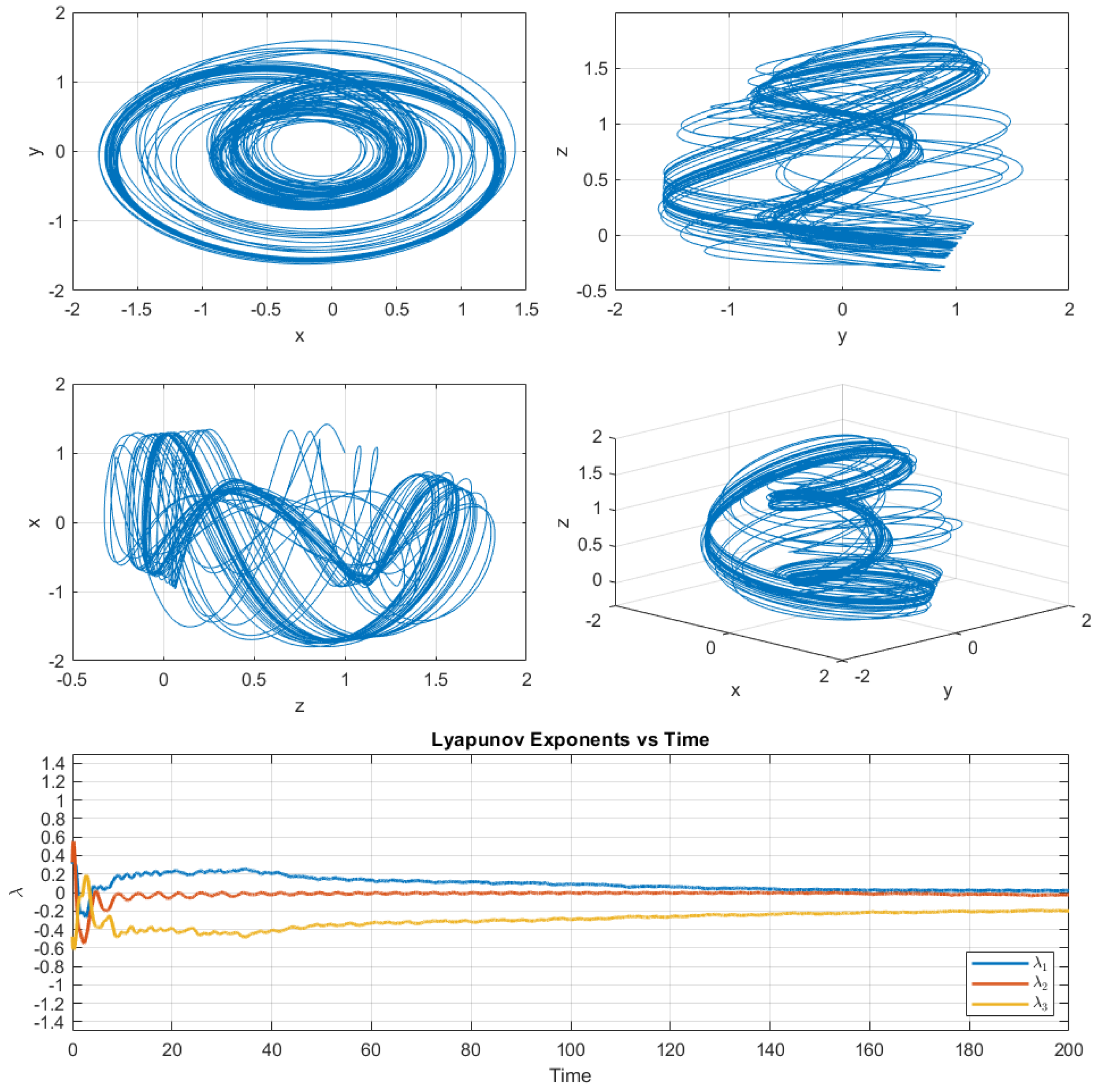
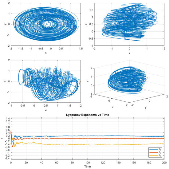
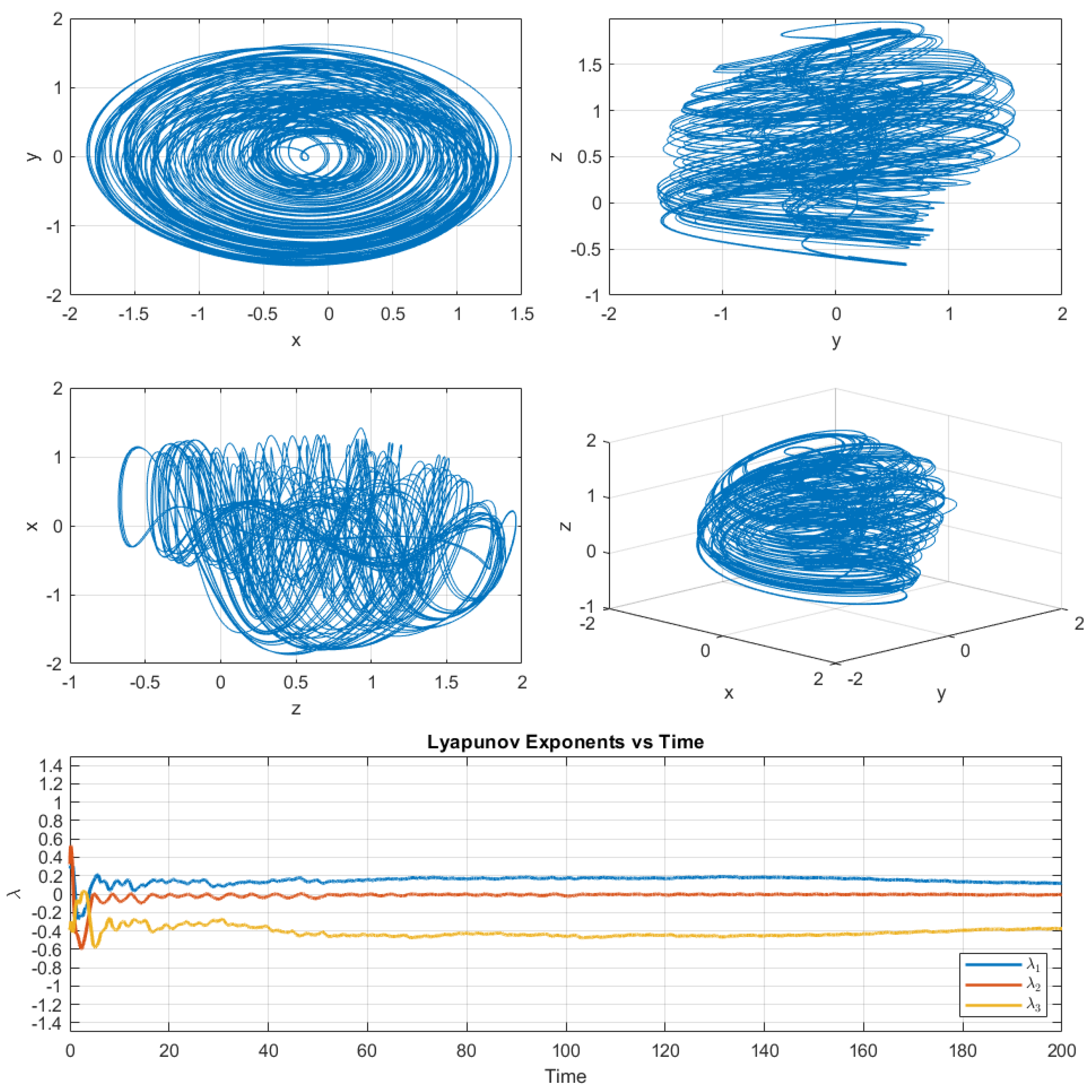
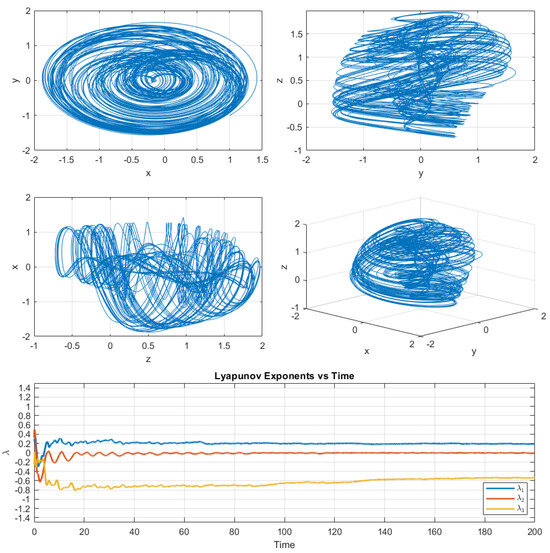
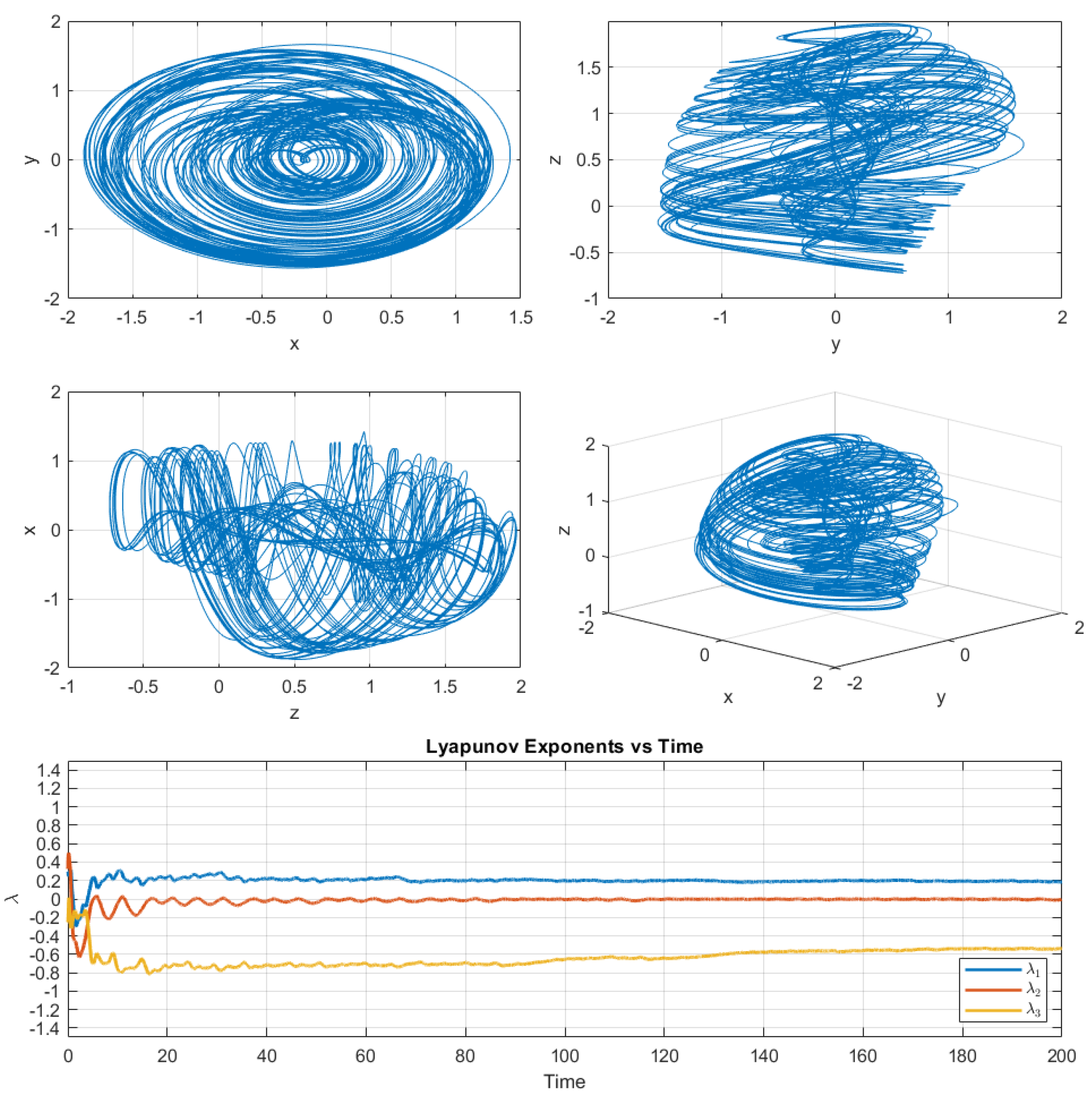
In this section, we are using a numerical approach to study the fractional-order Aizawa model. It is important to note that while Theorem 6 ensures local existence and uniqueness on $t\in [0,T_0]$ ($T_0\approx 0.495$ for $\tilde{\nu }=0.995$), the numerical simulations run over $t\in [0,200]$. Beyond $T_0$, the strict contractivity condition is relaxed, which is a necessary prerequisite for the emergence of the rich, non-periodic chaotic attractors observed in Figure 7, Figure 8, Figure 9, Figure 10, Figure 11, Figure 12, Figure 13, Figure 14 and Figure 15. We are approximating the Atangana–Baleanu (AB) fractional derivative using the two-step Lagrange polynomial method. This method allows us to efficiently approximate the resulting fractional dynamics while preserving the essential memory characteristics of the AB operator and enabling the generation of phase portraits and other numerical representations of the system. In our study of the fractional-order Aizawa system, we are evaluating the core dynamics by fixing several system parameters at their standard literature values to maintain consistent structural properties. The fixed (standard) parameters are a = 0.95, b = 0.70, c = 0.60, e = 0.25, initial condition $(1,-1,1)$, fractional derivative order $\tilde{\nu }=0.995$, time interval $t\in [0,200]$, and phase shift $h=0.01$. The initial condition plays a very important role in chaotic systems due to their high sensitivity to initial states. Even small disturbances can cause considerably different trajectories. Additionally, the computational interval of [0, 200] is sufficiently long to allow transient effects to diminish and to examine the long-term dynamics.

Figure 7. When $\gamma =3.0$ and $f=0.1$, the Lyapunov exponents’ plot and phase plots of $x-y,z-y,x-z,x-y-z$ are given.

Figure 8. When $\gamma =3.0$ and $f=0.2$, the Lyapunov exponents’ plot and phase plots of $x-y,z-y,x-z,x-y-z$ are given.

Figure 9. When $\gamma =3.0$ and $f=0.3$, the Lyapunov exponents’ plot and phase plots of $x-y,z-y,x-z,x-y-z$ are given.

Figure 10. When $\gamma =4.5$ and $f=0.1$, the Lyapunov exponents’ plot and phase plots of $x-y,z-y,x-z,x-y-z$ are given.

Figure 11. When $\gamma =4.5$ and $f=0.2$, the Lyapunov exponents’ plot and phase plots of $x-y,z-y,x-z,x-y-z$ are given.

Figure 12. When $\gamma =4.5$ and $f=0.3$, the Lyapunov exponents’ plot and phase plots of $x-y,z-y,x-z,x-y-z$ are given.

Figure 13. When $\gamma =4.9$ and $f=0.1$, the Lyapunov exponents’ plot and phase plots of $x-y,z-y,x-z,x-y-z$ are given.

Figure 14. When $\gamma =4.9$ and $f=0.2$, the Lyapunov exponents’ plot and phase plots of $x-y,z-y,x-z,x-y-z$ are given.

Figure 15. When $\gamma =4.9$ and $f=0.3$, the Lyapunov exponents’ plot and phase plots of $x-y,z-y,x-z,x-y-z$ are given.

As $z_3^{\ast }\approx -1.1328$ is a locally asymptotically stable axial equilibrium, the numerical simulations in Cases 1–9 are initialized at $(1,-1,1)$, which is not in the local neighborhood of this equilibrium. As a result, the local stability of $z_3^{\ast }$ does not imply the convergence of these trajectories to the equilibrium. Instead, the numerical trajectories exhibit bounded oscillatory and chaotic behavior. The nonlinear terms in the Aizawa system, particularly the cubic coupling term $fz{x}^3$, contribute to the nonlinear feedback that prevents unbounded growth and supports the formation of bounded chaotic attractors. In the fractional-order Aizawa model, the parameters $\gamma$ and f play a key role in directly affecting the system’s phase-space geometry and dynamic responses. Although $\gamma$ does not appear in the real parts of the eigenvalues $(Re({\mu }_{2,3})=z^{\ast }-b),$ it dictates the imaginary component $(Im({\mu }_{2,3})=\pm \gamma )$. Thus, varying $\gamma$ modulates the rotational frequency and phase mixing around the z-axis without altering the local stability nature or baseline geometry set by $a,b,c$.

The parameter f is responsible for scaling the nonlinear coupling term $fz{x}^3$, which in turn drives global trajectory stretching and folding, leading to chaos. We kept parameters a, b, and c fixed in order to maintain a consistent local structural framework, while varying $\gamma$ and f in order to systematically investigate rotational mixing and chaotic folding.

By making adjustments to these parameters, the final trajectory plots can show the transitions from steady-state convergence to complex periodic behavior and chaotic dynamics, providing a clear illustration of the impact of their variation. In all cases, for selected values for parameters $\gamma$ and $f,$ the Lyapunov-exponent graph for Lyapunov exponents $({\lambda }_1,{\lambda }_2,{\lambda }_3)$ are also shown. In all cases the positive value of ${\lambda }_1$ indicates exponential separation of initially nearby trajectories, while the negative exponent represents contraction in another direction. The corresponding divergence curve further demonstrates the sensitive dependence on initial conditions, whereas the bounded phase-space trajectory confirms that the observed divergence is associated with chaotic dynamics rather than unbounded instability. The following cases, along with their corresponding phase diagrams and Lyapunov exponent spectra, presented in Figure 7, Figure 8, Figure 9, Figure 10, Figure 11, Figure 12, Figure 13, Figure 14 and Figure 15, are constructed by varying the parameters $\gamma$ and f.

Case 1. 

When $\gamma$ is equal to 3 and f is equal to 0.1, we analyze the dynamics of the system and the Lyapunov exponents can be seen in Figure 7.

Case 2. 

When $\gamma$ is equal to 3 and f is equal to 0.2, we analyze the dynamics of the system and the Lyapunov exponents can be seen in Figure 8.

Case 3. 

When $\gamma$ is equal to 3 and f is equal to 0.3, we analyze the dynamics of the system and the Lyapunov exponents can be seen in Figure 9.

Case 4. 

When $\gamma$ is equal to 4.5 and f is equal to 0.1, we analyze the dynamics of the system and the Lyapunov exponents can be seen in Figure 10.

Case 5. 

When $\gamma$ is equal to 4.5 and f is equal to 0.2, we analyze the dynamics of the system and the Lyapunov exponents can be seen in Figure 11.

Case 6. 

When $\gamma$ is equal to 4.5 and f is equal to 0.3, we analyze the dynamics of the system and the Lyapunov exponents can be seen in Figure 12.

Case 7. 

When $\gamma$ is equal to 4.9 and f is equal to 0.1, we analyze the dynamics of the system and the Lyapunov exponents can be seen in Figure 13.

Case 8. 

When $\gamma$ is equal to 4.9 and f is equal to 0.2, we analyze the dynamics of the system and the Lyapunov exponents can be seen in Figure 14.

Case 9. 

When $\gamma$ is equal to 4.9 and f is equal to 0.3, we analyze the dynamics of the system and the Lyapunov exponents can be seen in Figure 15.

The Figure 7, Figure 8, Figure 9, Figure 10, Figure 11, Figure 12, Figure 13, Figure 14 and Figure 15 demonstrate the dynamic behavior of the system transitioning into chaos under the specified parameters in all above cases. The geometric attractor structure and Lyapunov spectrum both indicate the presence of deterministic chaos in this system, placing it within the broader category of nonlinear dynamical models. When looking at the x-y, z-y, and x-z projections, the trajectories do not converge into fixed points or periodic cycles. They fill specific areas with complex looping structures, which are a sign of a strange attractor. The three-dimensional representation highlights the fractal-like geometry, showcasing trajectories that undergo repeated stretching and folding. This mechanism aligns with the attractor dynamics seen in classical systems like the Lorenz attractor) and the Rössler system, where deterministic rules produce intricate, non-repetitive patterns.

The Lyapunov exponents offer a way to quantify stability in a system. When there is a positive exponent, it indicates that nearby trajectories are diverging exponentially, which is a key characteristic of chaos. A near-zero exponent represents a neutral direction in the system’s continuous time evolution, and negative exponents indicate contraction along other directions, keeping trajectories bounded. The mixed spectrum represents chaos through its deterministic yet unpredictable mathematical fingerprint.

Comparing can be possible with the Lorenz system, and both have a Lyapunov spectrum that includes one positive, one near-zero, and one negative exponent. This similarity emphasizes the widespread presence of chaotic dynamics. Ref. [23] highlighted that the balance of expansion and contraction is a defining characteristic of chaotic attractors, leading to bounded yet unpredictable trajectories.

8. Conclusions

A bicontrolled contractive framework has been developed in this work, which extends classical fixed-point theory. The authors introduced a new class of (F, B)-contractions governed by auxiliary functions, leading to the establishment of new fixed-point theorems that guarantee both the existence and uniqueness of solutions in complete metric spaces. The results of this study bring together and build upon previous contributions, including Banach’s contraction principle, Boyd–Wong’s generalization, and Reich’s extensions. They also offer a more adaptable structure for nonlinear mappings. To validate the theoretical framework, the study included illustrative examples and applied it to the fractional-order Aizawa system with the Atangana–Baleanu fractional derivative. The dynamical behavior of the system was confirmed through numerical simulations, graphical analysis, and Lyapunov exponents. These methods highlighted both convergence to fixed points and the emergence of chaotic trajectories under certain conditions. This demonstrates the richness of fractional dynamical systems and the significance of robust fixed-point techniques in analyzing them.

The current study suggests several potential areas for future research. One direction is to expand the bicontrolled $(F,B)$-contraction framework to encompass a wider range of metric structures, such as partial and probabilistic metric spaces. Another promising avenue is to apply these findings to fractional differential equations with nonlocal kernels, which are frequently encountered in physics and engineering. Additionally, the bicontrolled approach could offer valuable insights into equilibrium problems in economics and finance, where multiple nonlinear influences are at play. Finally, several directions remain open for further investigation. One important direction is the development of effective numerical and iterative methods for approximating fixed points of bicontrolled contractions, particularly in situations where the fixed point cannot be obtained explicitly. Such methods could include suitable iterative schemes together with computable error estimates, convergence rates, and stopping criteria. Another interesting direction is to investigate the applicability of bicontrolled contraction principles to nonlinear and fractional dynamical systems. In particular, it would be worthwhile to examine whether the proposed framework can be used to establish the existence and uniqueness of equilibria or other invariant states in systems exhibiting complex or chaotic behavior and to study the relationship between the contraction conditions and the resulting dynamical properties. These investigations could provide both theoretical extensions and computational applications of bicontrolled contraction theory.

References

- Banach, S. Sur les opérations dans les ensembles abstraits et leur application aux équations intégrales. Fundam. Math. 1922, 3, 133–181. [Google Scholar] [CrossRef] [Scilit]
- Rakotch, E. A note on contractive mappings. Proc. Am. Math. Soc. 1962, 13, 459–465. [Google Scholar] [CrossRef] [Scilit]
- Boyd, D.W.; Wong, J.S.W. On nonlinear contractions. Proc. Am. Math. Soc. 1969, 20, 458–464. [Google Scholar] [CrossRef] [Scilit]
- Ciric, L.B. A generalization of banach’s contraction principle. Proc. Am. Math. Soc. 1974, 45, 267–273. [Google Scholar] [CrossRef] [Scilit]
- Wardowski, D.; Dung, N.V. Fixed points of f-weak contractions on complete metric space. Demonstr. Math. 2014, 47, 146–155. [Google Scholar] [CrossRef] [Scilit]
- Wardowski, D. Fixed points of a new type of contractive mappings in complete metric spaces. Fixed Point Theory Appl. 2012, 94, 2012. [Google Scholar] [CrossRef] [Scilit]
- Proinov, P.D. Fixed point theorems for generalized contractive mappings in metric spaces. J. Fixed Point Theory Appl. 2020, 22, 21. [Google Scholar] [CrossRef] [Scilit]
- Agarwal, R.P.; Aksoy, U.; Karapınar, E.; Erhan, I. F-contraction mappings on metric-like spaces in connection with integral equations on time scales. Revista de la Real Academia de Ciencias Exactas Físicas y Naturales. Serie A. Matemáticas 2020, 114, 147. [Google Scholar] [CrossRef] [Scilit]
- Bedre, S. Remarks on f-weak contractions and discontinuity at the fixed point. Adv. Theory Nonlinear Anal. Appl. 2020, 4, 260–265. [Google Scholar] [CrossRef] [Scilit]
- Popescu, O.; Stan, G. Two fixed point theorems concerning f-contraction in complete metric spaces. Symmetry 2020, 12, 58. [Google Scholar] [CrossRef] [Scilit]
- Nazam, M.; Aydi, H.; Park, C.; Arshad, M.; Savas, E.; Shin, D.Y. Some variants of wardowski fixed point theorem. Adv. Differ. Equ. 2021, 2021, 485. [Google Scholar] [CrossRef] [Scilit]
- Ahmad, J.; Al-Rawashdeh, A.; Azam, A. New fixed point theorems for generalized f-contractions in complete metric spaces. Fixed Point Theory Appl. 2015, 80, 2015. [Google Scholar] [CrossRef] [Scilit]
- Alsulami, H.; Karapınar, E.; Piri, H. Fixed points of generalized f-suzuki type contraction in complete metric spaces. Discret. Dyn. Nat. Soc. 2015, 2015, 969726. [Google Scholar] [CrossRef] [Scilit]
- Reich, S. Some remarks concerning contraction mappings. Can. Math. Bull. 1971, 14, 121–124. [Google Scholar] [CrossRef] [Scilit]
- Suzuki, T. Several fixed point theorems for generalized contractions in complete metric spaces. Nonlinear Anal. Theory Methods Appl. 2005, 61, 455–463. [Google Scholar]
- Ahmad, H.; Din, F.U.; Younis, M. A novel Cirić–Reich–Rus fixed point approach for the existence and uniqueness criterion of a fractional-order Aizawa chaotic system. Chaos Solitons Fractals 2025, 200, 116932. [Google Scholar] [CrossRef] [Scilit]
- Jin, J.; Chen, W.; Ouyang, A.; Yu, F.; Liu, H. A time-varying fuzzy parameter zeroing neural network for the synchronization of chaotic systems. IEEE Trans. Emerg. Top. Comput. Intell. 2024, 8, 364–376. [Google Scholar] [CrossRef] [Scilit]
- Li, C.; Gao, Y.; Lei, T.; Li, R.Y.M.; Xu, Y. Two independent offset controllers in a three-dimensional chaotic system. Int. J. Bifurc. Chaos 2024, 34, 2450008. [Google Scholar] [CrossRef] [Scilit]
- Varan, M.; Ulusoy, B.; Pehlivan, I.; Gurevin, B.; Akgul, A. Nonlinear Analysis and Circuit Realization of Chaotic Aizawa System. In Proceedings of the International Conference on Applied Mathematics in Engineering (ICAME), Balikesir, Turkey, 27–29 June 2018; p. 191. [Google Scholar]
- Ghanbari, B.; Gómez-Aguilar, J.F. Two efficient numerical schemes for simulating dynamical systems and capturing chaotic behaviors with Mittag–Leffler memory. Eng. Comput. 2022, 38, 2139–2167. [Google Scholar] [CrossRef] [Scilit]
- Jain, S.; El-Khatib, Y. Modelling chaotic dynamical attractor with fractal-fractional differential operators. AIMS Math. 2021, 6, 13689–13725. [Google Scholar] [CrossRef] [Scilit]
- Echenausía-Monroy, J.L.; Magallón-García, D.A.; Ontañón-García, L.J.; Rivera Rodriguez, R.; Pena Ramirez, J.; Alvarez, J. Does a fractional-order recurrent neural network improve the identification of chaotic dynamics. Fractal Fract. 2024, 8, 632. [Google Scholar] [CrossRef] [Scilit]
- Ott, E. Chaos in Dynamical Systems, 2nd ed.; Cambridge University Press: Cambridge, UK, 2002. [Google Scholar]
Disclaimer/Publisher’s Note: The statements, opinions and data contained in all publications are solely those of the individual author(s) and contributor(s) and not of MDPI and/or the editor(s). MDPI and/or the editor(s) disclaim responsibility for any injury to people or property resulting from any ideas, methods, instructions or products referred to in the content. |
© 2026 by the authors. Licensee MDPI, Basel, Switzerland. This article is an open access article distributed under the terms and conditions of the Creative Commons Attribution (CC BY) license.