A Fractional Lotka–Volterra Predator–Prey Model with Strong Allee Effects, Nonlinear Harvesting, and Memory

Abstract

This work develops a fractional Lotka–Volterra predator–prey model incorporating a strong Allee effect, nonlinear anthropogenic harvesting, and memory-dependent dynamics through the Atangana–Baleanu–Caputo (ABC) fractional operator. The model describes the interactions between two prey populations and a predator under competition, predation, and nonlinear harvesting. Theoretical analysis establishes the existence and uniqueness, non-negativity, ultimate boundedness, and Ulam–Hyers stability of the solutions. Numerical simulations examine the effects of the fractional order $\varpi$, the characteristic time-scale $\tau$, the Allee-effect parameters, and harvesting effort. The results show that the fractional order modifies transient population dynamics, while $\tau$ regulates the fractional response through the factor ${\tau }^{1-\varpi }$. A systematic analysis of the Allee threshold $C_1$ reveals a sharp numerical persistence and extinction transition for the stronger prey, bracketed within $12.448<C_{1,\mathrm{tr}}<12.449$ for the prescribed parameter set and initial conditions, while the Allee severity parameter influences its temporal recovery. Increasing harvesting effort suppresses the prey populations and consequently affects the predator through trophic coupling, with fractional memory modifying the transient response. The proposed framework provides a flexible approach for investigating predator–prey dynamics under Allee effects, anthropogenic exploitation, and memory-dependent processes.

1. Introduction

The dynamical interplay between predator and prey has long served as a foundational concept in both theoretical and applied ecology, due to its essential function in modulating population abundances, structuring trophic networks, and upholding ecosystem resilience. In recent decades, the mathematical representation of predator-prey systems has garnered growing scholarly attention, providing a robust quantitative lens through which to interpret complex dynamical features, including local and global stability, cyclical fluctuations, bifurcation phenomena, and population collapse thresholds. The value of such modeling transcends purely theoretical pursuits, offering practical guidance for conserving biological diversity, sustainably managing natural resources, and anticipating ecological outcomes in response to changing environmental conditions.

A substantial body of research has focused on classical predator-prey models incorporating various biological mechanisms. Aguirre et al. [1] proposed an extended predator-prey model that includes an Allee effect on the prey and a ratio-dependent functional response. Their bifurcation analysis and numerical invariant manifold computations revealed the emergence or disappearance of limit cycles, homoclinic, and heteroclinic orbits near a Bogdanov-Takens bifurcation, thereby governing the global phase plane topology. Notably, they defined the Allee threshold as the basin boundary of an attracting positive equilibrium, providing precise conditions under which predator and prey either coexist or undergo mutual extinction.

Building upon such frameworks, subsequent studies have introduced additional ecological realism. Thirthar et al. [2] proposed a mammalian predator-prey model with logistic prey growth, Allee effects, and prey consumption shaped by water and moonlight. Their bifurcation analysis uncovered transcritical bifurcations tied to predator death rate and Hopf bifurcations tied to prey conversion rate. Their findings demonstrate that moonlight boosts hunting efficiency, water availability modulates system behavior, and a moderate Allee effect promotes stability through density-dependent mechanisms, while an excessive Allee effect drives instability and population crashes, with numerical simulations supporting these conclusions.

In addition to demographic and environmental factors, other ecological dimensions such as fear and migration have been extensively investigated. Yaseen et al. [3] studied fear and migration in a predator-prey model with an asymmetric functional response, where prey exhibit density-dependent anti-predator behavior that amplifies the fear effect. Existence conditions for all relevant equilibria were derived, and local and global dynamics were fully characterized. Modulating fear intensity and predator aggregate sensitivity produced diverse dynamical responses, with numerical simulations revealing that trait-mediated effects on prey growth, competition, fear, or death can destabilize the equilibrium, giving rise to periodic attractors.

To capture memory and hereditary dynamics intrinsic to biological systems, fractional calculus has increasingly been utilized to characterize complex predator-prey systems [4,5]. For instance, Lu et al. [6] demonstrated the significant impact of non-integer orders using a two-zone fishery model with Caputo derivatives. Ramesh et al. [7,8] examined fractional predator-prey frameworks incorporating memory, Allee effects, harvesting, and functional responses. Similarly, Kalra et al. [9] and Wang and Han analyzed multi-species food chains and refuge-dependent dynamics, showing how fractional frameworks alter stability and suppress chaos. Furthermore, Kumar et al. [10] utilized Caputo derivatives to highlight how varying fractional orders modify equilibrium stability under fear and predator mortality effects, with additional contributions found in [11,12,13].

Despite the broad application of fractional frameworks, many existing models overlook multi-prey interactions where predator preferences split between distinct biomass streams. A seminal integer-order framework addressing this multi-prey dynamic was established by Jana et al. [14], who investigated a predator–weaker prey–stronger prey model governed by the following system of equations:

$$\begin{array}{cc}\hfill {\displaystyle \frac{d{P}_1}{dt}}& =r_1{P}_1\left(1-{\displaystyle \frac{P_1}{A}}\right)-{\displaystyle \frac{\alpha P_1{P}_3}{a+P_1}}-{\eta }_1{P}_1{P}_2,\hfill \\ \hfill {\displaystyle \frac{d{P}_2}{dt}}& =r_2{P}_2\left(1-{\displaystyle \frac{P_2}{B}}\right)-\beta P_2{P}_3-{\eta }_2{P}_1{P}_2,\hfill \\ \hfill {\displaystyle \frac{d{P}_3}{dt}}& ={\displaystyle \frac{m_1\alpha P_1{P}_3}{a+P_1}}+m_2\beta P_2{P}_3-\delta P_3-\mu P_3^2,\hfill \end{array}$$

(1)

where $P_1$, $P_2$, and $P_3$ denote the biomass densities of the stronger prey, weaker prey, and predator species, respectively. The biological meanings of the remaining parameters are detailed in Table 1.

Table 1. Biological interpretation, dimensional units, and references of the FEEM (7) parameters.

Parameter	Meaning	Units	Source
$r_1,r_2$	Intrinsic growth rates of the stronger prey $P_1$ and weaker prey $P_2$, respectively	$1/\mathrm{time}$	[8,14]
$A,B$	Environmental carrying capacities of prey $P_1$ and prey $P_2$, respectively	$\mathrm{biomass}\mathrm{density}$	[8,14]
$\alpha ,\beta$	Predation-rate coefficients associated with predator $P_3$ on prey $P_1$ and prey $P_2$, respectively	$1/\mathrm{time}$	[14,15]
a	Half-saturation constant of the Holling Type II predatory functional response	$\mathrm{biomass}\mathrm{density}$	[14]
$m_1,m_2$	Biomass conversion efficiencies of prey $P_1$ and prey $P_2$ into predator $P_3$, respectively	dimensionless	[14]
${\eta }_1,{\eta }_2$	Interspecific competition coefficients between the two prey populations	$1/(\mathrm{biomass}\mathrm{density}·\mathrm{time})$	[14]
$\delta$	Natural mortality rate of the predator population $P_3$	$1/\mathrm{time}$	[8,14]
$\mu$	Intraspecific self-limitation coefficient of the predator population $P_3$	$1/(\mathrm{biomass}\mathrm{density}·\mathrm{time})$	[14]
$C_1$	Allee threshold for the stronger prey population $P_1$	$\mathrm{biomass}\mathrm{density}$	[8]
$C_2$	Positive scaling parameter determining the shape of the Allee-effect response for $P_1$	$\mathrm{biomass}\mathrm{density}$	[8]
$q_1,q_2$	Harvesting-efficiency (catchability) coefficients for prey $P_1$ and prey $P_2$, respectively	$1/\mathrm{time}$	[15]
$E_1,E_2$	Applied harvesting effort directed toward prey $P_1$ and prey $P_2$, respectively	$\mathrm{harvesting}\mathrm{effort}$	[15]
$u_1,u_2$	Dimensionless saturation coefficients associated with harvesting effort	dimensionless	[15]
$v_1,v_2$	Coefficients converting prey biomass density into the effort-equivalent quantity in the harvesting denominator	$\mathrm{effort}/\mathrm{biomass}\mathrm{density}$	[15]
$\tau$	Characteristic time-scale parameter introduced to ensure dimensional compatibility of the fractional model	time	Assumed

Despite its valuable contribution to multi-species dynamics, the model proposed by Jana et al. [14] exhibits several notable limitations. First, it assumes standard logistic growth for both prey populations without incorporating Allee effects, which critically influence population persistence and extinction thresholds at low densities [8]. Second, it neglects harvesting strategies on the prey species, despite harvesting being a vital intervention for population control and commercial management [16,17]. Third, because the model relies on classical integer-order derivatives, it inherently fails to capture memory and hereditary properties. Addressing these limitations through a fractional-order formulation provides a more accurate representation of real-world ecological dynamics, particularly for conservation planning and long-term population forecasting.

To address the aforementioned limitations, the present work extends the model of Jana et al. [14] through several key modifications. First, we incorporate a strong Allee effect term $\left({\displaystyle \frac{P_1-C_1}{P_1+C_2}}\right)$ into the growth rate of the stronger prey $P_1$, where $C_1$ denotes the longevity or persistence threshold of the prey and $C_2$ is an auxiliary parameter [18,19], thereby capturing the reduced per-capita growth rate at low population densities. Second, we introduce a Michaelis–Menten type multi-species harvesting function defined as $h_k(P_k,E_k)=q_k{\displaystyle \frac{E_k{P}_k}{u_k{E}_k+v_k{P}_k}}$ for $k\in \{1,2\}$, where $q_k$ is the catchability coefficient, $E_k$ is the harvesting effort, and $u_k,v_k>0$ are constants. This harvesting formulation is widely recognized as biologically and economically realistic [15,16,17,20], with the biological significance of $u_k$ and $v_k$ detailed in Section 3 of [16]. Third, we reformulate the extended model using the Atangana–Baleanu–Caputo (ABC) fractional derivative to construct the Fractional Extended Ecological Model (FEEM), which possesses a non-singular and non-local kernel capable of capturing memory effects and hereditary properties that classical integer-order derivatives cannot represent. By coupling these mechanisms within a multi-prey predator–prey framework, the proposed FEEM enables their combined influence on population persistence, anthropogenic exploitation, and memory-dependent dynamics to be examined within a unified system. The resulting numerical analysis identifies model-specific dynamical responses, including an abrupt persistence and extinction transition associated with the Allee threshold and memory-dependent modification of the transient response to harvesting.

The remainder of this article is structured as follows. Section 2 introduces the fundamental concepts of fractional calculus and the Atangana–Baleanu fractional integral operator used in the proposed framework. Section 3 formulates the Fractional Extended Ecological Model (FEEM), incorporating the strong Allee effect, nonlinear Michaelis–Menten-type harvesting, interspecific competition, predator–prey interactions, and memory-dependent dynamics. Section 4 presents the main theoretical results, including the existence and uniqueness of solutions, non-negativity, ultimate boundedness, and Ulam–Hyers stability of the proposed system. Section 5 presents the numerical implementation and sensitivity analyses, examining the effects of the fractional order, the characteristic time-scale, the strong Allee-effect parameters, and anthropogenic harvesting on the temporal dynamics of the three populations. Finally, Section 6 summarizes the main conclusions of the study and outlines future directions of the proposed model.

2. Some Basic Definitions

The present section delineates the requisite mathematical preliminaries, systematically formalizing the fundamental definitions of fractional integrals and derivatives while emphasizing the significance of their associated memory kernels. A comprehensive exposition of the recently introduced Atangana–Baleanu fractional derivatives (ABFD), characterized by their distinctive non-singular and non-local kernel properties, is subsequently provided. These operators serve as the analytical foundation that supports the derivation and proof of the principal findings in the sections that follow.

Definition 1 

([21]). Consider $\varpi >0$. The Riemann–Liouville fractional integral (RLFI) of order ϖ for a function $\varphi \left(t\right)$ is defined by

$$0^{\mathcal{RL}}{\mathbf{I}}_t^{\varpi }\varphi \left(t\right)={\left(\Gamma \left(\varpi \right)\right)}^{-1}{\int }_0^t{(t-\xi )}^{\varpi -1}\varphi \left(\xi \right)d\xi ,$$

(2)

where $\varphi \left(t\right)\in L^1(0,T)$ with $T<\infty$.

Definition 2 

([21]). For any real number ϖ satisfying $0<\varpi <1$, the Caputo fractional derivative (CFD) of order ϖ for a function $\varphi \left(t\right)$ takes the form

$${}_0{}^{\mathcal{C}}\mathbf{D}_t^{\varpi }\varphi \left(t\right)={\left(\Gamma (1-\varpi )\right)}^{-1}{\int }_0^t{(t-\xi )}^{-\varpi }{\varphi }^{\prime }\left(\xi \right)d\xi ,$$

(3)

whenever ${\varphi }^{\prime }\left(t\right)\in L^1(0,T)$, where ${\varphi }^{\prime }\left(t\right)$ denotes the ordinary derivative of $\varphi \left(t\right)$.

Definition 3 

([22,23,24]). Suppose ϖ is a real number confined to the interval $(0,1)$. The Caputo-type Atangana–Baleanu fractional derivative (ABFD) of order ϖ for a function $\varphi \left(t\right)$ is given by

$$0^{\mathcal{ABC}}{\mathbf{D}}_t^{\varpi }\varphi \left(t\right)={\displaystyle \frac{\mathcal{N}\left(\varpi \right)}{1-\varpi }}{\int }_0^t{\mathbf{E}}_{\varpi }\left(-{\kappa }_{\varpi }{(t-\xi )}^{\varpi }\right){\varphi }^{\prime }\left(\xi \right)d\xi ,$$

(4)

wherein ${\kappa }_{\varpi }={\displaystyle \frac{\varpi }{1-\varpi }}$ represents a scaling (relaxation) parameter. The quantity $\mathcal{N}\left(\varpi \right)$ denotes a normalization function satisfying $\mathcal{N}\left(0\right)=\mathcal{N}\left(1\right)=1$. Here, ${\varphi }^{\prime }\left(\xi \right)\in L^1(0,T)$ signifies the ordinary derivative of $\varphi \left(\xi \right)$, and ${\mathbf{E}}_{\varpi }\left(z\right)$ is the Mittag–Leffler function defined as ${\mathbf{E}}_{\varpi }\left(z\right)={\sum }_{j=0}^{\infty }{\displaystyle \frac{z^j}{\Gamma (\varpi j+1)}},$ with $\mathcal{ABC}$ denoting the Atangana–Baleanu operator in the Caputo sense.

Remark 1. 

It is worth mentioning that at the boundary limits $\varpi \to 0^{+}$ and $\varpi \to 1^{-}$, the operators recover the traditional base states such that ${}_0{}^{\mathcal{C}}\mathbf{D}_t^0\varphi \left(t\right)=0^{\mathcal{ABC}}{\mathbf{D}}_t^0\varphi \left(t\right)=\varphi \left(t\right)-\varphi \left(0\right)$ and ${}_0{}^{\mathcal{C}}\mathbf{D}_t^1\varphi \left(t\right)=0^{\mathcal{ABC}}{\mathbf{D}}_t^1\varphi \left(t\right)={\varphi }^{\prime }\left(t\right)$, respectively. Furthermore, within the Caputo-type Atangana–Baleanu fractional derivative (ABFD), the scaling parameter ${\kappa }_{\varpi }={\displaystyle \frac{\varpi }{1-\varpi }}$ appears inside the Mittag–Leffler kernel ${\mathcal{M}}_{\varpi }\left(-{\kappa }_{\varpi }{(t-\xi )}^{\varpi }\right)$. This parameter ensures proper kernel normalization and facilitates a gradual transition of the memory component between short-term and long-term influences. More precisely, ${\kappa }_{\varpi }$ acts as a relaxation coefficient: for sufficiently small ϖ, it produces gradual decay (long memory), while as ϖ approaches 1, ${\kappa }_{\varpi }$ increases substantially, localizing the kernel near the current state and recovering the ordinary first derivative. Thus, ${\kappa }_{\varpi }$ modulates the contribution of past states in a manner consistent with the integral formulation while capturing both Markovian and non-Markovian dynamical behaviors.

Definition 4 

([22,23]). The Atangana–Baleanu fractional integral (ABFI) operator, which corresponds to the fractional derivative defined in Definition 3, is formulated as

$$0^{\mathcal{ABC}}{\mathcal{I}}_t^{\varpi }\varphi \left(t\right)={\displaystyle \frac{1-\varpi }{\mathcal{N}\left(\varpi \right)}}\varphi \left(t\right)+{\displaystyle \frac{\varpi }{\mathcal{N}\left(\varpi \right)\Gamma \left(\varpi \right)}}{\int }_0^t{(t-\xi )}^{\varpi -1}\varphi \left(\xi \right)d\xi ,$$

(5)

wherein $\mathcal{N}\left(\varpi \right)$ denotes the normalization mapping that satisfies $\mathcal{N}\left(0\right)=\mathcal{N}\left(1\right)=1$, and $\Gamma (·)$ represents the standard Gamma function.

Lemma 1 

([22,23,24]). Let ϖ be a real number satisfying $0<\varpi <1$, and let ${\varphi }^{\prime }\left(t\right)\in L^1(0,T)$. Then, for the Atangana–Baleanu fractional integral (ABFI) operator $0^{\mathcal{ABC}}{\mathcal{I}}_t^{\varpi }$ as defined in Definition 4 and the associated Atangana–Baleanu fractional derivative (ABFD) operator $0^{\mathcal{ABC}}{\mathbf{D}}_t^{\varpi }$ as defined in Definition 3, the following relationship holds true:

$$0^{\mathcal{ABC}}{\mathcal{I}}_t^{\varpi }\left(0^{\mathcal{ABC}}{\mathbf{D}}_t^{\varpi }\varphi \left(t\right)\right)=\varphi \left(t\right)-\varphi \left(0\right).$$

Lemma 2 

([21,22,23]). The Laplace transform associated with the Atangana–Baleanu fractional derivative (ABFD) from Definition 3 satisfies

$$\mathcal{L}\left\{0^{\mathcal{ABC}}{\mathbf{D}}_t^{\varpi }\varphi \left(t\right)\right\}\left(q\right)={\displaystyle \frac{\mathcal{N}\left(\varpi \right)\left(q^{\varpi }\Phi \left(q\right)-q^{\varpi -1}\varphi \left(0\right)\right)}{\varpi +(1-\varpi )q^{\varpi }}},$$

(6)

where $\Phi \left(q\right)=\mathcal{L}\left\{\varphi \right(t\left)\right\}\left(q\right)$ denotes the Laplace transform of $\varphi \left(t\right)$.

Definition 5 

([5,25]). Consider a mapping ${\mathcal{F}:(\mathcal{U},\parallel ·\parallel }_{\mathcal{U}}{)\to (\mathcal{V},\parallel ·\parallel }_{\mathcal{V}})$ defined between two normed linear spaces. The mapping $\mathcal{F}$ is said to be Hyers–Ulam stable if there exists a positive constant $c>0$ such that, for every $ϵ>0$, any v belonging to the range of $\mathcal{F}$, and any $u\in \mathcal{U}$ satisfying ${\parallel v-\mathcal{F}\left(u\right)\parallel }_{\mathcal{V}}<ϵ$, one can find an element $u_0\in \mathcal{U}$ with $\mathcal{F}\left(u_0\right)=v$ and $\parallel u_0{-u\parallel }_{\mathcal{U}}<cϵ$.

In the sequel, let $\mathcal{J}=[0,T]$ where T is a finite positive real number. We consider the Banach space $\mathcal{X}\left(\mathcal{J}\right)$ consisting of all continuous real-valued functions defined on $\mathcal{J}$, endowed with the norm $\parallel P\parallel :={sup}_{t\in \mathcal{J}}\left|P\left(t\right)\right|,P\in \mathcal{X}\left(\mathcal{J}\right).$ For the present three-species ecological model, we set $m=3$ and introduce the product Banach space $\mathcal{P}={\left(\mathcal{X}\left(\mathcal{J}\right)\right)}^3.$ An arbitrary element of $\mathcal{P}$ is denoted by $\mathbf{X}={(P_1,P_2,P_3)}^{\top }\in \mathcal{P}.$ We equip $\mathcal{P}$ with the maximum product norm ${\parallel \mathbf{X}\parallel }_{\mathcal{P}}={max}_{1\le j\le 3}\parallel P_j\parallel .$ Since $\mathcal{J}$ is a compact interval and each $P_j\in C(\mathcal{J},\mathbb{R})$, every component function $P_j$ is bounded on $\mathcal{J}$. Consequently, the supremum norms appearing above are finite. Moreover, $\mathcal{P}$ is a Banach space under the norm ${\parallel ·\parallel }_{\mathcal{P}}$. This functional-analytic framework provides the appropriate setting for the qualitative analysis of the proposed fractional-order ecological model.

3. Model Assumptions and Formulation

In this section, we formulate the proposed fractional Lotka–Volterra-type predator–prey model by extending the integer-order multi-prey framework in (1). The proposed formulation incorporates three additional mechanisms: a strong Allee effect in the stronger prey population, nonlinear harvesting of both prey populations, and memory effects through the Atangana–Baleanu–Caputo (ABC) fractional derivative. These mechanisms are introduced to account, respectively, for low-density limitations on prey persistence, anthropogenic extraction, and the influence of past population states on the present dynamics.

• We incorporate a strong Allee effect into the per-capita growth rate of the stronger prey population $\left(P_1\right)$ through the dimensionless factor ${\displaystyle \frac{P_1-C_1}{P_1+C_2}},$ where $(C_1>0)$ denotes the Allee threshold and $(C_2>0)$ is a scaling parameter that determines the shape of the Allee-effect response. Since the ratio must be dimensionless, both $\left(C_1\right)$ and $\left(C_2\right)$ have the same units as the biomass density $\left(P_1\right)$. In particular, the factor becomes negative when $(0\le P_1<C_1)$, representing the reduced growth and increased extinction tendency associated with sufficiently low prey density [8].
• We introduce a nonlinear harvesting function for each prey population, defined by $h_k(P_k,E_k)=q_k{\displaystyle \frac{E_k{P}_k}{u_k{E}_k+v_k{P}_k}},k\in \{1,2\},$ where $\left(P_k\right)$ denotes the biomass density of prey $\left(k\right)$, $(E_k>0)$ represents the corresponding harvesting effort, and $(q_k>0)$ is a harvesting-efficiency coefficient. The positive parameters $\left(u_k\right)$ and $\left(v_k\right)$ determine the relative contributions of harvesting effort and prey biomass to the saturation mechanism. The parameters are assigned appropriate dimensions so that $\left(u_k{E}_k\right)$ and $\left(v_k{P}_k\right)$ have the same units, while $\left(h_k\right)$ has the units of a population-rate term. The nonlinear form allows harvesting to increase with prey biomass and harvesting effort while exhibiting saturation effects.
• We reformulate the extended model by employing the Atangana–Baleanu–Caputo (ABC) fractional derivative, represented by the operator $0^{\mathcal{ABC}}{\mathbf{D}}_t^{\varpi }$. This fractional formulation accounts for nonlocal memory and hereditary effects that cannot be represented by the classical integer-order derivative.

Based on the above modifications, we propose the following Fractional Extended Ecological Model (FEEM):

$$\left\{\begin{array}{cc}\hfill 0^{\mathcal{ABC}}{\mathbf{D}}_t^{\varpi }{P}_1\left(t\right)& ={\tau }^{1-\varpi }\left[r_1{P}_1\left(t\right)\left(1-{\displaystyle \frac{P_1\left(t\right)}{A}}\right)\left({\displaystyle \frac{P_1\left(t\right)-C_1}{P_1\left(t\right)+C_2}}\right)-{\displaystyle \frac{\alpha P_1\left(t\right)P_3\left(t\right)}{a+P_1\left(t\right)}}-{\eta }_1{P}_1\left(t\right)P_2\left(t\right)-h_1(P_1\left(t\right),E_1)\right],\hfill \\ \hfill 0^{\mathcal{ABC}}{\mathbf{D}}_t^{\varpi }{P}_2\left(t\right)& ={\tau }^{1-\varpi }\left[r_2{P}_2\left(t\right)\left(1-{\displaystyle \frac{P_2\left(t\right)}{B}}\right)-\beta P_2\left(t\right)P_3\left(t\right)-{\eta }_2{P}_1\left(t\right)P_2\left(t\right)-h_2(P_2\left(t\right),E_2)\right],\hfill \\ \hfill 0^{\mathcal{ABC}}{\mathbf{D}}_t^{\varpi }{P}_3\left(t\right)& ={\tau }^{1-\varpi }\left[{\displaystyle \frac{m_1\alpha P_1\left(t\right)P_3\left(t\right)}{a+P_1\left(t\right)}}+m_2\beta P_2\left(t\right)P_3\left(t\right)-\delta P_3\left(t\right)-\mu P_3^2\left(t\right)\right],\hfill \end{array}\right.$$

(7)

where $\tau >0$ serves as a finite characteristic time-scale parameter, while the factor ${\tau }^{1-\varpi }$ ensures dimensional compatibility between the ecological rate terms and the fractional-order dynamics. The harvesting functions are explicitly given by

$$h_1(P_1,E_1)=q_1{\displaystyle \frac{E_1{P}_1}{u_1{E}_1+v_1{P}_1}},h_2(P_2,E_2)=q_2{\displaystyle \frac{E_2{P}_2}{u_2{E}_2+v_2{P}_2}}.$$

The system is supplemented with the nonnegative initial conditions

$$P_1\left(0\right)=P_{10}\ge 0,P_2\left(0\right)=P_{20}\ge 0,P_3\left(0\right)=P_{30}\ge 0,$$

(8)

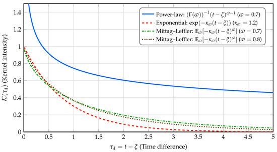
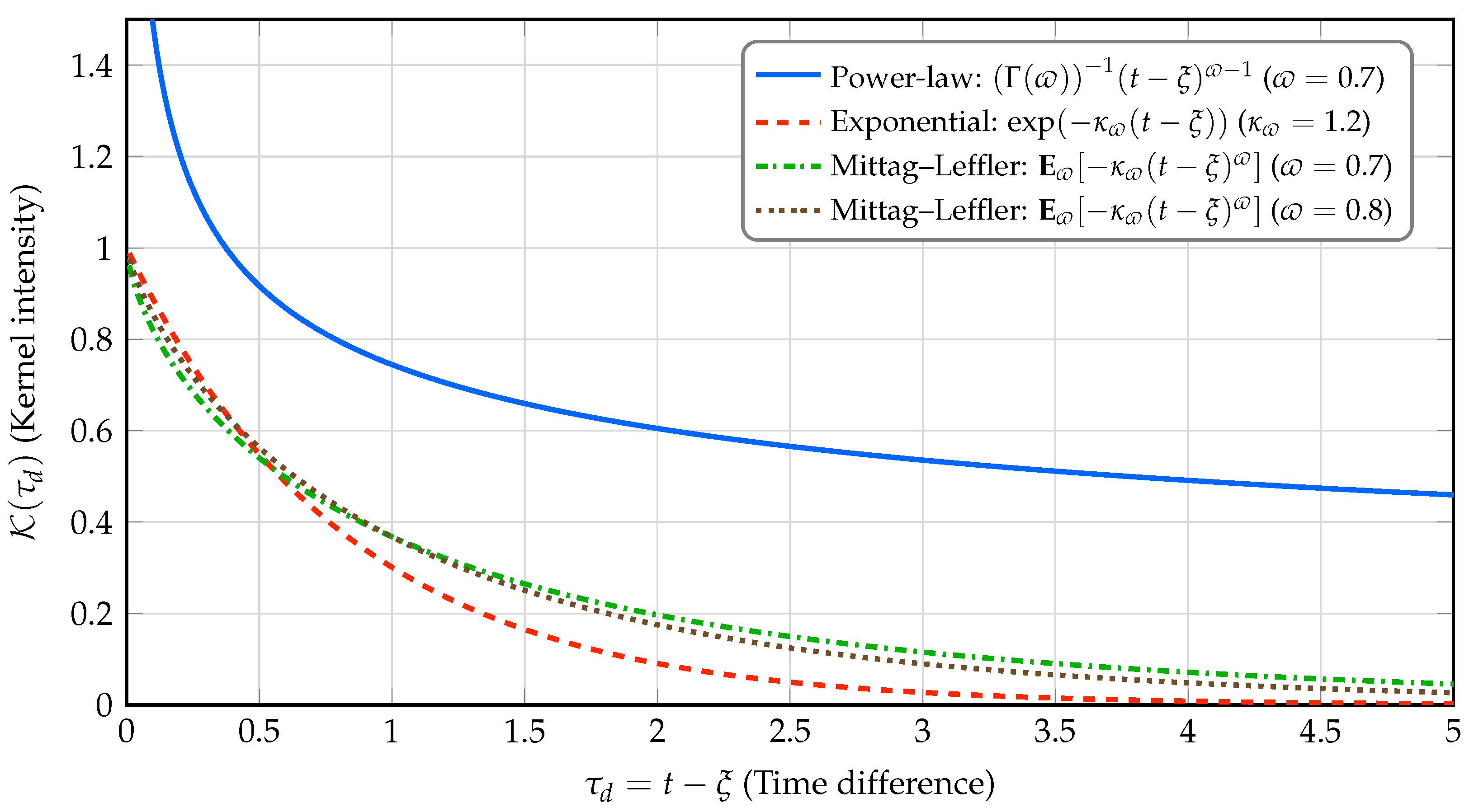
In contrast to classical integer-order models, which describe population dynamics through instantaneous rates of change, the fractional order $\varpi$ introduces a nonlocal temporal dependence that accounts for the influence of past system states. The Atangana–Baleanu–Caputo (ABC) operator is employed because of its non-singular Mittag–Leffler kernel, which provides a fading-memory representation without the singular kernel associated with conventional power-law fractional derivatives, as illustrated in Figure 1. Consequently, the model incorporates historical effects into the evolution of the interacting populations rather than relying solely on their instantaneous states.

Figure 1. Comparison of power-law, exponential, and Mittag–Leffler kernels for fractional orders $\varpi =0.7$ and $\varpi =0.8$. Note that the power-law kernel displays normalized intensity using the scaling coefficient $1/\Gamma \left(0.7\right)\approx 0.7447$ to strictly comply with the Riemann–Liouville integral definition. The Mittag–Leffler kernel smoothly interpolates between power-law and exponential decay profiles, making it exceptionally suited for modeling memory-dependent ecological phenomena.

To clarify the ecological terminology and the structural assumptions of the proposed framework, the dynamic roles of the two prey populations and the harvesting mechanisms are briefly specified. Following the foundational multi-prey model [14], the designations stronger prey ($P_1$) and weaker prey ($P_2$) reflect their different predator–prey interaction mechanisms: $P_1$ is considered the principal prey resource and is therefore subjected to the stronger predation mechanism, in addition to interspecific competition with $P_2$. This ecological setting motivates the incorporation of a strong Allee effect exclusively into the $P_1$ population, representing density-dependent limitations that may become critical when its abundance falls below a persistence threshold. In contrast, $P_2$ is modeled without an Allee effect and serves as an alternative prey population. Thus, the asymmetric treatment of the two prey species is intended to reflect their distinct functional roles and interaction mechanisms within the predator–prey community.

Furthermore, anthropogenic harvesting effort is explicitly incorporated into the dynamics of both prey populations, whereas direct harvesting of the apex predator $P_3$ is omitted. This modeling choice reflects an ecological management framework in which anthropogenic extraction is primarily directed toward lower trophic levels, while direct exploitation of the apex predator is not considered. For $k\in \{1,2\}$, the harvesting rate is described by the nonlinear function $h_k(P_k,E_k)=q_k{\displaystyle \frac{E_k{P}_k}{u_k{E}_k+v_k{P}_k}},$ which is increasing in both prey biomass and harvesting effort and incorporates diminishing returns through its saturating structure. Larger values of $q_k$ represent greater harvesting efficiency or catchability. The parameter $u_k$ regulates the contribution of harvesting effort to the saturation mechanism; when $u_k{E}_k\gg v_k{P}_k$, the harvesting rate approaches $h_k(P_k,E_k)\approx {\displaystyle \frac{q_k}{u_k}}{P}_k.$ Conversely, when $v_k{P}_k\gg u_k{E}_k$, the harvesting rate approaches $h_k(P_k,E_k)\approx {\displaystyle \frac{q_k}{v_k}}{E}_k,$ and becomes approximately independent of prey biomass. Hence, the relative magnitudes of $u_k{E}_k$ and $v_k{P}_k$ determine the transition between the two limiting harvesting regimes, providing a flexible framework for examining the effects of nonlinear resource extraction and its potential cascading consequences across trophic levels [16,17].

The proposed FEEM therefore retains the fundamental ecological structure of the multi-prey predator–prey framework of Jana et al. [14], while extending it through the incorporation of a strong Allee effect, nonlinear harvesting, and fractional memory. These extensions introduce additional factors that may influence population persistence and dynamical behavior, particularly the Allee threshold $C_1$, harvesting efforts $E_1$ and $E_2$, and the fractional parameters $\varpi$ and $\tau$. Unlike the model of Singh and Malik [15], which considers a two-species Leslie–Gower predator–prey system with Michaelis–Menten prey harvesting and a discrete-time formulation, the present model considers two prey populations and one predator within a continuous-time fractional framework and incorporates a strong Allee effect and harvesting of both prey populations. The qualitative implications of these extensions and their differences from the results reported in [14,15] are examined in the subsequent analysis.

4. Qualitative Analysis of the FEEM

This section investigates the principal qualitative properties of the proposed FEEM (7). First, we establish the existence and uniqueness of solutions by converting the fractional system into an equivalent Volterra-type integral formulation and verifying suitable Lipschitz conditions. We then establish the non-negativity of the population variables, thereby ensuring the biological feasibility of the model. Subsequently, we derive an ultimate boundedness result to demonstrate the dissipative behavior of the system. Finally, we establish Ulam–Hyers stability, thereby quantifying the robustness of the model with respect to admissible perturbations. These qualitative results provide the mathematical foundation for the numerical simulations presented in the subsequent sections, where the effects of the fractional order, Allee threshold, and nonlinear harvesting mechanisms on the predator–prey dynamics are explored.

4.1. Existence and Uniqueness via the Volterra Integral Formulation

We establish the existence and uniqueness of solutions for the proposed FEEM (7) on a finite time interval $\mathcal{J}=[0,T]$, where $T>0$. The analysis is based on the integral representation associated with the Atangana–Baleanu–Caputo operator. By applying the corresponding Atangana–Baleanu fractional integral, the fractional differential system is transformed into an equivalent Volterra-type integral system. We then establish a Lipschitz estimate for the nonlinear operator in the maximum product norm, by estimating its components separately, taking into account the strong Allee effect, predator–prey interactions, interspecific competition, and nonlinear harvesting terms. These estimates will be used to derive the contraction condition required to establish the existence and uniqueness of the solution on $\mathcal{J}$. Applying the Atangana–Baleanu fractional integral operator $0^{\mathcal{ABC}}{\mathcal{I}}_t^{\varpi }$ to the FEEM (7) and using the corresponding initial conditions yields the following equivalent integral representation:

$$\left\{\begin{array}{cc}\hfill P_1\left(t\right)& =P_{10}+{\tau }^{1-\varpi }{0}^{\mathcal{ABC}}{\mathcal{I}}_t^{\varpi }\left\{r_1{P}_1\left(t\right)\left(1-{\displaystyle \frac{P_1\left(t\right)}{A}}\right)\left({\displaystyle \frac{P_1\left(t\right)-C_1}{P_1\left(t\right)+C_2}}\right)-{\displaystyle \frac{\alpha P_1\left(t\right)P_3\left(t\right)}{a+P_1\left(t\right)}}-{\eta }_1{P}_1\left(t\right)P_2\left(t\right)-h_1(P_1\left(t\right),E_1)\right\},\hfill \\ \hfill P_2\left(t\right)& =P_{20}+{\tau }^{1-\varpi }{0}^{\mathcal{ABC}}{\mathcal{I}}_t^{\varpi }\left\{r_2{P}_2\left(t\right)\left(1-{\displaystyle \frac{P_2\left(t\right)}{B}}\right)-\beta P_2\left(t\right)P_3\left(t\right)-{\eta }_2{P}_1\left(t\right)P_2\left(t\right)-h_2(P_2\left(t\right),E_2)\right\},\hfill \\ \hfill P_3\left(t\right)& =P_{30}+{\tau }^{1-\varpi }{0}^{\mathcal{ABC}}{\mathcal{I}}_t^{\varpi }\left\{{\displaystyle \frac{m_1\alpha P_1\left(t\right)P_3\left(t\right)}{a+P_1\left(t\right)}}+m_2\beta P_2\left(t\right)P_3\left(t\right)-\delta P_3\left(t\right)-\mu P_3^2\left(t\right)\right\}.\hfill \end{array}\right.$$

(9)

Define the nonlinear component operators ${\Theta }_i$, $i=1,2,3$, by the nonlinear right-hand sides of the three equations in (7). For $\mathbf{X}\left(t\right)={(P_1\left(t\right),P_2\left(t\right),P_3\left(t\right))}^{\top }$, we have $\Theta \left(\mathbf{X}\left(t\right)\right)={\left({\Theta }_1\left(\mathbf{X}\left(t\right)\right),{\Theta }_2\left(\mathbf{X}\left(t\right)\right),{\Theta }_3\left(\mathbf{X}\left(t\right)\right)\right)}^{\top }\in \mathcal{P},$ where

$$\left\{\begin{array}{cc}\hfill {\Theta }_1\left(\mathbf{X}\left(t\right)\right)& =r_1{P}_1\left(t\right)\left(1-{\displaystyle \frac{P_1\left(t\right)}{A}}\right)\left({\displaystyle \frac{P_1\left(t\right)-C_1}{P_1\left(t\right)+C_2}}\right)-{\displaystyle \frac{\alpha P_1\left(t\right)P_3\left(t\right)}{a+P_1\left(t\right)}}-{\eta }_1{P}_1\left(t\right)P_2\left(t\right)-h_1(P_1\left(t\right),E_1),\hfill \\ \hfill {\Theta }_2\left(\mathbf{X}\left(t\right)\right)& =r_2{P}_2\left(t\right)\left(1-{\displaystyle \frac{P_2\left(t\right)}{B}}\right)-\beta P_2\left(t\right)P_3\left(t\right)-{\eta }_2{P}_1\left(t\right)P_2\left(t\right)-h_2(P_2\left(t\right),E_2),\hfill \\ \hfill {\Theta }_3\left(\mathbf{X}\left(t\right)\right)& ={\displaystyle \frac{m_1\alpha P_1\left(t\right)P_3\left(t\right)}{a+P_1\left(t\right)}}+m_2\beta P_2\left(t\right)P_3\left(t\right)-\delta P_3\left(t\right)-\mu P_3^2\left(t\right).\hfill \end{array}\right.$$

(10)

Using the definition of the Atangana–Baleanu fractional integral, the integral representation (9) can be written explicitly as the following Volterra-type integral system:

$$\left\{\begin{array}{cc}\hfill P_1\left(t\right)& =P_{10}+{\displaystyle \frac{(1-\varpi ){\tau }^{1-\varpi }}{\mathcal{N}\left(\varpi \right)}}{\Theta }_1\left(\mathbf{X}\left(t\right)\right)+{\displaystyle \frac{\varpi {\tau }^{1-\varpi }}{\mathcal{N}\left(\varpi \right)\Gamma \left(\varpi \right)}}{\int }_0^t{(t-\psi )}^{\varpi -1}{\Theta }_1\left(\mathbf{X}\left(\psi \right)\right)d\psi ,\hfill \\ \hfill P_2\left(t\right)& =P_{20}+{\displaystyle \frac{(1-\varpi ){\tau }^{1-\varpi }}{\mathcal{N}\left(\varpi \right)}}{\Theta }_2\left(\mathbf{X}\left(t\right)\right)+{\displaystyle \frac{\varpi {\tau }^{1-\varpi }}{\mathcal{N}\left(\varpi \right)\Gamma \left(\varpi \right)}}{\int }_0^t{(t-\psi )}^{\varpi -1}{\Theta }_2\left(\mathbf{X}\left(\psi \right)\right)d\psi ,\hfill \\ \hfill P_3\left(t\right)& =P_{30}+{\displaystyle \frac{(1-\varpi ){\tau }^{1-\varpi }}{\mathcal{N}\left(\varpi \right)}}{\Theta }_3\left(\mathbf{X}\left(t\right)\right)+{\displaystyle \frac{\varpi {\tau }^{1-\varpi }}{\mathcal{N}\left(\varpi \right)\Gamma \left(\varpi \right)}}{\int }_0^t{(t-\psi )}^{\varpi -1}{\Theta }_3\left(\mathbf{X}\left(\psi \right)\right)d\psi .\hfill \end{array}\right.$$

(11)

Since the nonlinear functions in (10) are continuously differentiable on their admissible domain, they are locally Lipschitz continuous. In particular, on any prescribed closed and bounded rectangular set containing the initial data, the corresponding partial derivatives are bounded, and hence explicit Lipschitz constants can be obtained. More precisely, let $\Omega =[0,M_1]\times [0,M_2]\times [0,M_3],M_i>0,i=1,2,3,$ be a prescribed closed and bounded rectangular subset of ${\mathbb{R}}_{+}^3$ containing the initial state ${\mathbf{X}}_0={(P_{10},P_{20},P_{30})}^{\top }$ and assume that $\mathbf{X}={(P_1,P_2,P_3)}^{\top },\overline{\mathbf{X}}={({\overline{P}}_1,{\overline{P}}_2,{\overline{P}}_3)}^{\top }$ belong to $\Omega$. Then

$$\left|{\Theta }_i\left(\mathbf{X}\left(t\right)\right)-{\Theta }_i\left(\overline{\mathbf{X}}\left(t\right)\right)\right|\le L_i{∥\mathbf{X}-\overline{\mathbf{X}}∥}_{\mathcal{P}},\mathbf{X},\overline{\mathbf{X}}\in \mathcal{P},t\in \mathcal{J},i=1,2,3.$$

(12)

where component bounds $L_i$ are given by

$$\begin{array}{cc}\hfill L_1& =r_1\left[\left(1+{\displaystyle \frac{2M_1}{A}}\right)\left(1+{\displaystyle \frac{C_1}{C_2}}\right)+M_1\left(1+{\displaystyle \frac{M_1}{A}}\right){\displaystyle \frac{C_1+C_2}{C_2^2}}\right]+{\displaystyle \frac{\alpha M_3}{a}}+{\eta }_1{M}_2+{\displaystyle \frac{q_1}{u_1}}+{\eta }_1{M}_1+\alpha ,\hfill \\ \hfill L_2& =r_2\left(1+{\displaystyle \frac{2M_2}{B}}\right)+\beta M_3+{\eta }_2{M}_1+{\displaystyle \frac{q_2}{u_2}}+{\eta }_2{M}_2+\beta M_2,\hfill \\ \hfill L_3& ={\displaystyle \frac{m_1\alpha M_3}{a}}+m_2\beta M_3+{\displaystyle \frac{m_1\alpha M_1}{a}}+m_2\beta M_2+\delta +2\mu M_3.\hfill \end{array}$$

(13)

Theorem 1. 

Let $L={max}_{1\le i\le 3}{L}_i,$ where $L_1,L_2,L_3$ are the Lipschitz constants obtained in the preceding estimates (13). Then, the FEEM (7) admits a unique solution $\mathbf{X}\left(t\right)\in \mathcal{P}$ on $\mathcal{J}$, provided that $\Xi \left(\tau \right)<1,$ where $\Xi \left(\tau \right)=\left({\displaystyle \frac{1-\varpi }{\mathcal{N}\left(\varpi \right)}}+{\displaystyle \frac{T^{\varpi }}{\mathcal{N}\left(\varpi \right)\Gamma \left(\varpi \right)}}\right)L{\tau }^{1-\varpi }.$

Proof. 

For $k\in \mathbb{N}$, we construct the sequence ${\left\{{\mathbf{X}}_k\left(t\right)\right\}}_{k\in \mathbb{N}}$ using the recursive formula derived from (11):

$$\begin{array}{cc}\hfill P_{i,k}\left(t\right)& =P_{i,0}+{\displaystyle \frac{(1-\varpi ){\tau }^{1-\varpi }}{\mathcal{N}\left(\varpi \right)}}{\Theta }_i\left({\mathbf{X}}_{k-1}\left(t\right)\right)+{\displaystyle \frac{\varpi {\tau }^{1-\varpi }}{\mathcal{N}\left(\varpi \right)\Gamma \left(\varpi \right)}}{\int }_0^t{(t-\psi )}^{\varpi -1}{\Theta }_i\left({\mathbf{X}}_{k-1}\left(\psi \right)\right)d\psi ,\hfill \end{array}$$

(14)

where ${\mathbf{X}}_{k-1}\left(t\right)={\left(P_{1,k-1}\left(t\right),P_{2,k-1}\left(t\right),P_{3,k-1}\left(t\right)\right)}^{\top },$ and the initial baseline approximation is given by $P_{i,0}\left(t\right)=P_{i,0},t\in \mathcal{J},i=1,2,3.$ Let ${\Lambda }_k\left(t\right)={\mathbf{X}}_k\left(t\right)-{\mathbf{X}}_{k-1}\left(t\right),k\ge 1,$ denote the difference between two consecutive iterates. Equivalently, ${\Lambda }_{i,k}\left(t\right)=P_{i,k}\left(t\right)-P_{i,k-1}\left(t\right).$ Using (14), for $k\ge 2$ we obtain

$$\begin{array}{cc}\hfill {\Lambda }_{i,k}\left(t\right)& ={\displaystyle \frac{(1-\varpi ){\tau }^{1-\varpi }}{\mathcal{N}\left(\varpi \right)}}\left[{\Theta }_i\left({\mathbf{X}}_{k-1}\left(t\right)\right)-{\Theta }_i\left({\mathbf{X}}_{k-2}\left(t\right)\right)\right]\hfill \\ \hfill & +{\displaystyle \frac{\varpi {\tau }^{1-\varpi }}{\mathcal{N}\left(\varpi \right)\Gamma \left(\varpi \right)}}{\int }_0^t{(t-\psi )}^{\varpi -1}\left[{\Theta }_i\left({\mathbf{X}}_{k-1}\left(\psi \right)\right)-{\Theta }_i\left({\mathbf{X}}_{k-2}\left(\psi \right)\right)\right]d\psi .\hfill \end{array}$$

(15)

Taking the absolute value and applying the triangle inequality, we have

$$\begin{array}{cc}\hfill |{\Lambda }_{i,k}\left(t\right)|& \le {\displaystyle \frac{(1-\varpi ){\tau }^{1-\varpi }}{\mathcal{N}\left(\varpi \right)}}\left|{\Theta }_i\left({\mathbf{X}}_{k-1}\left(t\right)\right)-{\Theta }_i\left({\mathbf{X}}_{k-2}\left(t\right)\right)\right|\hfill \\ \hfill & +{\displaystyle \frac{\varpi {\tau }^{1-\varpi }}{\mathcal{N}\left(\varpi \right)\Gamma \left(\varpi \right)}}{\int }_0^t{(t-\psi )}^{\varpi -1}\left|{\Theta }_i\left({\mathbf{X}}_{k-1}\left(\psi \right)\right)-{\Theta }_i\left({\mathbf{X}}_{k-2}\left(\psi \right)\right)\right|d\psi .\hfill \end{array}$$

(16)

Using the Lipschitz condition (12) with $\mathbf{X}={\mathbf{X}}_{k-1}$ and $\overline{\mathbf{X}}={\mathbf{X}}_{k-2}$, we obtain

$$\begin{array}{cc}\hfill |{\Lambda }_{i,k}\left(t\right)|& \le {\displaystyle \frac{(1-\varpi ){\tau }^{1-\varpi }}{\mathcal{N}\left(\varpi \right)}}{L}_i{∥{\mathbf{X}}_{k-1}-{\mathbf{X}}_{k-2}∥}_{\mathcal{P}}\hfill \\ \hfill & +{\displaystyle \frac{\varpi {\tau }^{1-\varpi }{L}_i}{\mathcal{N}\left(\varpi \right)\Gamma \left(\varpi \right)}}{∥{\mathbf{X}}_{k-1}-{\mathbf{X}}_{k-2}∥}_{\mathcal{P}}{\int }_0^t{(t-\psi )}^{\varpi -1}d\psi .\hfill \end{array}$$

(17)

Since ${\mathbf{X}}_{k-1}-{\mathbf{X}}_{k-2}={\Lambda }_{k-1}$, the preceding inequality becomes

$$\begin{array}{cc}\hfill |{\Lambda }_{i,k}\left(t\right)|& \le {\displaystyle \frac{(1-\varpi ){\tau }^{1-\varpi }}{\mathcal{N}\left(\varpi \right)}}{L}_i{∥{\Lambda }_{k-1}∥}_{\mathcal{P}}\hfill \\ \hfill & +{\displaystyle \frac{\varpi {\tau }^{1-\varpi }{L}_i}{\mathcal{N}\left(\varpi \right)\Gamma \left(\varpi \right)}}{∥{\Lambda }_{k-1}∥}_{\mathcal{P}}{\int }_0^t{(t-\psi )}^{\varpi -1}d\psi .\hfill \end{array}$$

(18)

Taking the supremum over $t\in \mathcal{J}$ and using ${\int }_0^t{(t-\psi )}^{\varpi -1}d\psi \le {\displaystyle \frac{T^{\varpi }}{\varpi }},$ we obtain

$$\begin{array}{cc}\hfill \underset{t\in \mathcal{J}}{sup}\left|{\Lambda }_{i,k}\left(t\right)\right|& \le \left({\displaystyle \frac{1-\varpi }{\mathcal{N}\left(\varpi \right)}}+{\displaystyle \frac{T^{\varpi }}{\mathcal{N}\left(\varpi \right)\Gamma \left(\varpi \right)}}\right)L_i{\tau }^{1-\varpi }{∥{\Lambda }_{k-1}∥}_{\mathcal{P}}.\hfill \end{array}$$

(19)

Define ${\Xi }_i\left(\tau \right)=\left({\displaystyle \frac{1-\varpi }{\mathcal{N}\left(\varpi \right)}}+{\displaystyle \frac{T^{\varpi }}{\mathcal{N}\left(\varpi \right)\Gamma \left(\varpi \right)}}\right)L_i{\tau }^{1-\varpi }.$ Since $L_i\le L$, we have ${\Xi }_i\left(\tau \right)\le \Xi \left(\tau \right),$ where $\Xi \left(\tau \right)=\left({\displaystyle \frac{1-\varpi }{\mathcal{N}\left(\varpi \right)}}+{\displaystyle \frac{T^{\varpi }}{\mathcal{N}\left(\varpi \right)\Gamma \left(\varpi \right)}}\right)L{\tau }^{1-\varpi }.$ Consequently, taking the maximum over $i=1,2,3$ gives

$${∥{\Lambda }_k∥}_{\mathcal{P}}\le \Xi \left(\tau \right){∥{\Lambda }_{k-1}∥}_{\mathcal{P}},k\ge 2.$$

(20)

By induction, it follows that

$${∥{\Lambda }_k∥}_{\mathcal{P}}\le {\left(\Xi \left(\tau \right)\right)}^{k-1}{∥{\Lambda }_1∥}_{\mathcal{P}},k\ge 1.$$

(21)

For any integer $\overline{m}>0$ and $k\ge 1$, we consider the difference between two successive approximations separated by $\overline{m}$ iterations. By the triangle inequality,

$$\begin{array}{cc}\hfill {∥{\mathbf{X}}_{k+\overline{m}}-{\mathbf{X}}_k∥}_{\mathcal{P}}& \le {\displaystyle \sum _{s=1}^{\overline{m}}}{∥{\Lambda }_{k+s}∥}_{\mathcal{P}}\hfill \\ \hfill & \le {∥{\Lambda }_1∥}_{\mathcal{P}}{\displaystyle \sum _{s=1}^{\overline{m}}}{\left(\Xi \left(\tau \right)\right)}^{k+s-1}\hfill \\ \hfill & ={∥{\Lambda }_1∥}_{\mathcal{P}}{\left(\Xi \left(\tau \right)\right)}^k{\displaystyle \sum _{s=0}^{\overline{m}-1}}{\left(\Xi \left(\tau \right)\right)}^s\hfill \\ \hfill & ={∥{\Lambda }_1∥}_{\mathcal{P}}{\left(\Xi \left(\tau \right)\right)}^k{\displaystyle \frac{1-{\left(\Xi \left(\tau \right)\right)}^{\overline{m}}}{1-\Xi \left(\tau \right)}}.\hfill \end{array}$$

(22)

Since $0\le \Xi \left(\tau \right)<1$ by hypothesis, the right-hand side tends to zero as $k\to \infty$. Hence, ${\left\{{\mathbf{X}}_k\right\}}_{k\in \mathbb{N}}$ is a Cauchy sequence in the complete Banach space $\mathcal{P}$. Therefore, there exists ${\mathbf{X}}^{\ast }\left(t\right)={\left(P_1^{\ast }\left(t\right),P_2^{\ast }\left(t\right),P_3^{\ast }\left(t\right)\right)}^{\top }\in \mathcal{P}$ such that ${\mathbf{X}}_k\left(t\right)⟶{\mathbf{X}}^{\ast }\left(t\right)$ uniformly on $\mathcal{J}$. Since the operators ${\Theta }_i$ are continuous on the prescribed domain and the sequence $\left\{{\mathbf{X}}_k\right\}$ converges uniformly, we may pass to the limit in (14). Thus,

$$\begin{array}{cc}\hfill P_i^{\ast }\left(t\right)& =P_{i,0}+{\displaystyle \frac{(1-\varpi ){\tau }^{1-\varpi }}{\mathcal{N}\left(\varpi \right)}}{\Theta }_i\left({\mathbf{X}}^{\ast }\left(t\right)\right)+{\displaystyle \frac{\varpi {\tau }^{1-\varpi }}{\mathcal{N}\left(\varpi \right)\Gamma \left(\varpi \right)}}{\int }_0^t{(t-\psi )}^{\varpi -1}{\Theta }_i\left({\mathbf{X}}^{\ast }\left(\psi \right)\right)d\psi ,\hfill \end{array}$$

(23)

for $i=1,2,3$. Hence, ${\mathbf{X}}^{\ast }\left(t\right)$ satisfies the integral system (11). By the equivalence between (11) and the FEEM (7), ${\mathbf{X}}^{\ast }\left(t\right)$ is a solution of the model. It remains to establish uniqueness. Suppose that $\mathbf{X}\left(t\right)$ and $\mathbf{Y}\left(t\right)$ are two solutions of (7). Subtracting their corresponding integral equations and applying the same Lipschitz estimate as above gives

$$\begin{array}{cc}\hfill {∥\mathbf{X}-\mathbf{Y}∥}_{\mathcal{P}}& \le \left({\displaystyle \frac{1-\varpi }{\mathcal{N}\left(\varpi \right)}}+{\displaystyle \frac{T^{\varpi }}{\mathcal{N}\left(\varpi \right)\Gamma \left(\varpi \right)}}\right)L{\tau }^{1-\varpi }{∥\mathbf{X}-\mathbf{Y}∥}_{\mathcal{P}}=\Xi \left(\tau \right){∥\mathbf{X}-\mathbf{Y}∥}_{\mathcal{P}}.\hfill \end{array}$$

(24)

Consequently, $\left(1-\Xi \left(\tau \right)\right){∥\mathbf{X}-\mathbf{Y}∥}_{\mathcal{P}}\le 0.$ Since $\Xi \left(\tau \right)<1$, we have $1-\Xi \left(\tau \right)>0$, and therefore ${∥\mathbf{X}-\mathbf{Y}∥}_{\mathcal{P}}=0.$ Thus, $\mathbf{X}\left(t\right)=\mathbf{Y}\left(t\right),t\in \mathcal{J},$ which proves uniqueness. Hence, the FEEM (7) admits a unique solution on $\mathcal{J}$. □

4.2. Forward Invariance and Non-Negativity of Solutions

This subsection establishes the non-negativity of the state trajectories, which is a prerequisite for the ecological validity of the FEEM. Since the state variables $P_i\left(t\right)$, $i=1,2,3$, represent physical biomass densities, negative values are biologically inadmissible. We therefore show that the non-negative orthant

$${\mathbb{R}}_{+}^3=\left\{(P_1,P_2,P_3)\in {\mathbb{R}}^3:P_1\ge 0,P_2\ge 0,P_3\ge 0\right\}$$

is a forward-invariant region for the FEEM. Consequently, solutions starting from non-negative initial data remain in the biologically meaningful state space throughout their evolution.

Lemma 3. 

Consider the FEEM (7) with non-negative initial conditions $P_{10}\ge 0, P_{20}\ge 0, P_{30}\ge 0.$ Then the non-negative orthant ${\mathbb{R}}_{+}^3$ is forward invariant for the FEEM (7) on $\mathcal{J}=[0,T]$. In particular, $P_1\left(t\right)\ge 0, P_2\left(t\right)\ge 0, P_3\left(t\right)\ge 0,t\in \mathcal{J}.$

Proof. 

We prove that the non-negative orthant is forward invariant on $\mathcal{J}=[0,T]$. Suppose, to the contrary, that a solution starting from ${\mathbb{R}}_{+}^3$ leaves the non-negative orthant at some time in $\mathcal{J}$. Since the solution components are continuous, there exists a first time $t_1\in (0,T]$ at which at least one component reaches the boundary of ${\mathbb{R}}_{+}^3$ and attempts to cross into the negative region, while all components remain non-negative on $[0,t_1]$.

The argument is based on the fractional minimum principle for fractional differential equations involving Mittag–Leffler-type kernels; see Al-Refai [26]. At the first boundary contact, the component that reaches zero attains a non-positive minimum. The fractional minimum principle then implies that, under a genuine attempted crossing into the negative region, the corresponding Atangana–Baleanu–Caputo derivative must be strictly negative.

We first consider the boundary $P_1\left(t_1\right)=0$. Since $P_2\left(t_1\right),P_3\left(t_1\right)\ge 0$, every term in the first component of the nonlinear operator contains either the factor $P_1\left(t_1\right)$ or the harvesting term $h_1(P_1\left(t_1\right),E_1)$. Moreover, because $E_1>0$, $h_1(0,E_1)=0.$ Consequently, ${\Theta }_1\left(\mathbf{X}\left(t_1\right)\right)=0.$ Hence, by the first equation of (7), $0^{\mathcal{ABC}}{\mathcal{D}}_t^{\varpi }{P}_1\left(t_1\right)={\tau }^{1-\varpi }{\Theta }_1\left(\mathbf{X}\left(t_1\right)\right)=0.$ This contradicts the strict inequality furnished by the fractional minimum principle at a first boundary crossing.

Next, suppose that $P_2\left(t_1\right)=0.$ Since $P_1\left(t_1\right),P_3\left(t_1\right)\ge 0$, every term in the second component of the nonlinear operator contains the factor $P_2\left(t_1\right)$ or the harvesting term $h_2(P_2\left(t_1\right),E_2)$. Because $E_2>0$, $h_2(0,E_2)=0.$ Therefore, ${\Theta }_2\left(\mathbf{X}\left(t_1\right)\right)=0,$ and the second equation of (7) gives $0^{\mathcal{ABC}}{\mathcal{D}}_t^{\varpi }{P}_2\left(t_1\right)={\tau }^{1-\varpi }{\Theta }_2\left(\mathbf{X}\left(t_1\right)\right)=0,$ again contradicting the fractional minimum principle.

Finally, suppose that $P_3\left(t_1\right)=0.$ Since $P_1\left(t_1\right),P_2\left(t_1\right)\ge 0$, every term in the third component of the nonlinear operator contains the factor $P_3\left(t_1\right)$. Hence, ${\Theta }_3\left(\mathbf{X}\left(t_1\right)\right)=0,$ and therefore, from the third equation of (7), $0^{\mathcal{ABC}}{\mathcal{D}}_t^{\varpi }{P}_3\left(t_1\right)={\tau }^{1-\varpi }{\Theta }_3\left(\mathbf{X}\left(t_1\right)\right)=0.$ This again contradicts the fractional minimum principle at a first boundary crossing.

Thus, none of the three components can cross any coordinate boundary from the non-negative region into the negative region. Therefore, $P_1\left(t\right)\ge 0,P_2\left(t\right)\ge 0,P_3\left(t\right)\ge 0,t\in \mathcal{J}.$ Consequently, $\mathbf{X}\left(t\right)\in {\mathbb{R}}_{+}^3,t\in \mathcal{J},$ and hence ${\mathbb{R}}_{+}^3$ is a forward-invariant region for the FEEM. This completes the proof. □

Remark 2. 

The non-negativity result allows zero initial biomass, but the structure of the FEEM implies that a population initially absent cannot be generated spontaneously by the model. Indeed, if $P_{i0}=0$ for some $i\in \{1,2,3\}$, then ${\Theta }_i\left(\mathbf{X}\left(t\right)\right){|}_{P_i=0}=0,$ because all terms in the respective component contain $P_i$ or the corresponding harvesting term $h_i(P_i,E_i)$, with $h_i(0,E_i)=0$. Thus, under the uniqueness established in Theorem (1), the corresponding coordinate hyperplanes are invariant. In particular, $P_{i0}=0\Rightarrow P_i\left(t\right)\equiv 0$ for $i=1,2,3.$ Hence, a population that is initially absent remains absent, and the corresponding lower-dimensional subsystem describes the resulting ecological dynamics. For the full three-species FEEM considered in the subsequent analysis and numerical simulations, we therefore take $P_{i0}>0$ for $i=1,2,3,$ while retaining the more general non-negative conditions $P_{i0}\ge 0$ ($i=1,2,3$) in the mathematical formulation of the model.

4.3. Boundedness of Solutions in the FEEM

For continuous-time ecological models, confirming the boundedness of solutions is essential to verify both mathematical integrity and biological plausibility. Whereas positivity prevents population densities from assuming physically inadmissible negative values, boundedness ensures that no state variable exhibits unbounded growth, which would be inconsistent with ecological reality. Ecosystems are inherently constrained by limited resources, carrying capacities, and competitive interactions. By demonstrating that the total weighted biomass of the fractional-order system remains bounded within a compact region, we confirm that the model respects these environmental limitations and precludes unphysical population divergence driven by the non-local memory dynamics.

Lemma 4. 

Assume that the state variables of the FEEM (7) are initialized with $P_i\left(0\right)>0$ for all $i\in \{1,2,3\}$. Then, the FEEM (7) is globally bounded on $\mathcal{J}$ and ultimately bounded by the weighted biomass threshold ${\displaystyle \frac{{\mathcal{M}}_0}{\delta }},$ where ${\mathcal{M}}_0={\displaystyle \frac{A{\left(r_1^{\ast }+\delta \right)}^2}{4r_1}}+{\displaystyle \frac{m_{2}B{(r_2+\delta )}^2}{4m_1{r}_2}},$ with $r_1^{\ast }=r_1\left(1+{\displaystyle \frac{C_1+C_2}{A}}\right).$

Proof. 

Let us define the total weighted environmental biomass function

$$Z\left(t\right)=P_1\left(t\right)+{\displaystyle \frac{m_2}{m_1}}{P}_2\left(t\right)+{\displaystyle \frac{1}{m_1}}{P}_3\left(t\right).$$

(25)

By the linearity of the Atangana–Baleanu–Caputo derivative,

$$0^{\mathcal{ABC}}{\mathcal{D}}_t^{\varpi }Z\left(t\right)=0^{\mathcal{ABC}}{\mathcal{D}}_t^{\varpi }{P}_1\left(t\right)+{\displaystyle \frac{m_2}{m_1}}{0}^{\mathcal{ABC}}{\mathcal{D}}_t^{\varpi }{P}_2\left(t\right)+{\displaystyle \frac{1}{m_1}}{0}^{\mathcal{ABC}}{\mathcal{D}}_t^{\varpi }{P}_3\left(t\right).$$

(26)

Substituting the three equations of the FEEM (7) into (26), then cancel the predator–prey interaction terms gives

$$\begin{array}{cc}\hfill 0^{\mathcal{ABC}}{\mathcal{D}}_t^{\varpi }Z\left(t\right)& ={\tau }^{1-\varpi }[r_1{P}_1\left(1-{\displaystyle \frac{P_1}{A}}\right)\left({\displaystyle \frac{P_1-C_1}{P_1+C_2}}\right)-{\eta }_1{P}_1{P}_2-h_1(P_1,E_1)\hfill \\ \hfill & +{\displaystyle \frac{m_2}{m_1}}{r}_2{P}_2\left(1-{\displaystyle \frac{P_2}{B}}\right)-{\displaystyle \frac{m_2}{m_1}}{\eta }_2{P}_1{P}_2-{\displaystyle \frac{m_2}{m_1}}{h}_2(P_2,E_2)-{\displaystyle \frac{\delta }{m_1}}{P}_3-{\displaystyle \frac{\mu }{m_1}}{P}_3^2].\hfill \end{array}$$

(27)

To justify the upper estimate for the strong Allee-effect growth term, observe that, for $P_1\ge 0$,

$$\begin{array}{cc}& \left(1+{\displaystyle \frac{C_1+C_2}{A}}-{\displaystyle \frac{P_1}{A}}\right)-\left(1-{\displaystyle \frac{P_1}{A}}\right)\left({\displaystyle \frac{P_1-C_1}{P_1+C_2}}\right)\hfill \\ & ={\displaystyle \frac{(A+C_2)(C_1+C_2)}{A(P_1+C_2)}}>0.\hfill \end{array}$$

Therefore,

$$r_1{P}_1\left(1-{\displaystyle \frac{P_1}{A}}\right)\left({\displaystyle \frac{P_1-C_1}{P_1+C_2}}\right)\le r_1^{\ast }{P}_1-{\displaystyle \frac{r_1}{A}}{P}_1^2,$$

(28)

where

$$r_1^{\ast }=r_1\left(1+{\displaystyle \frac{C_1+C_2}{A}}\right).$$

(29)

Moreover, because $E_1,E_2>0$ and the harvesting parameters are positive, the harvesting functions satisfy $h_1(P_1,E_1)\ge 0, h_2(P_2,E_2)\ge 0$ for all $P_1,P_2\ge 0$. By the previously established non-negativity of the population trajectories, we have $P_1\left(t\right),P_2\left(t\right),P_3\left(t\right)\ge 0,t\in \mathcal{J}.$ Consequently, $-{\eta }_1{P}_1{P}_2\le 0,-{\displaystyle \frac{m_2}{m_1}}{\eta }_2{P}_1{P}_2\le 0,$ $-h_1(P_1,E_1)\le 0,-{\displaystyle \frac{m_2}{m_1}}{h}_2(P_2,E_2)\le 0,$ and $-{\displaystyle \frac{\mu }{m_1}}{P}_3^2\le 0.$ Combining these estimates with (28), we obtain the following fractional differential inequality:

$$\begin{array}{cc}\hfill 0^{\mathcal{ABC}}{\mathcal{D}}_t^{\varpi }Z\left(t\right)\le {\tau }^{1-\varpi }& [r_1^{\ast }{P}_1\left(t\right)-{\displaystyle \frac{r_1}{A}}{P}_1^2\left(t\right)+{\displaystyle \frac{m_2}{m_1}}\left(r_2{P}_2\left(t\right)-{\displaystyle \frac{r_2}{B}}{P}_2^2\left(t\right)\right)-{\displaystyle \frac{\delta }{m_1}}{P}_3\left(t\right)].\hfill \end{array}$$

(30)

Adding ${\tau }^{1-\varpi }\delta Z\left(t\right)$ to both sides of (30) gives

$$\begin{array}{cc}\hfill 0^{\mathcal{ABC}}{\mathcal{D}}_t^{\varpi }Z\left(t\right)+{\tau }^{1-\varpi }\delta Z\left(t\right)\le {\tau }^{1-\varpi }& \left[\right(r_1^{\ast }+\delta )P_1-{\displaystyle \frac{r_1}{A}}{P}_1^2+{\displaystyle \frac{m_2}{m_1}}\left((r_2+\delta )P_2-{\displaystyle \frac{r_2}{B}}{P}_2^2\right)].\hfill \end{array}$$

(31)

The quadratic expressions on the right-hand side attain their maximum values for $P_1,P_2\ge 0$ at $P_1={\displaystyle \frac{A(r_1^{\ast }+\delta )}{2r_1}},P_2={\displaystyle \frac{B(r_2+\delta )}{2r_2}},$ respectively. Hence,

$$\underset{P_1\ge 0}{max}\left[(r_1^{\ast }+\delta )P_1-{\displaystyle \frac{r_1}{A}}{P}_1^2\right]={\displaystyle \frac{A{(r_1^{\ast }+\delta )}^2}{4r_1}},$$

and

$$\underset{P_2\ge 0}{max}\left[(r_2+\delta )P_2-{\displaystyle \frac{r_2}{B}}{P}_2^2\right]={\displaystyle \frac{B{(r_2+\delta )}^2}{4r_2}}.$$

Therefore, define

$${\mathcal{M}}_0={\displaystyle \frac{A{(r_1^{\ast }+\delta )}^2}{4r_1}}+{\displaystyle \frac{m_{2}B{(r_2+\delta )}^2}{4m_1{r}_2}}.$$

(32)

It follows from (31) that

$$0^{\mathcal{ABC}}{\mathcal{D}}_t^{\varpi }Z\left(t\right)+{\tau }^{1-\varpi }\delta Z\left(t\right)\le {\tau }^{1-\varpi }{\mathcal{M}}_0.$$

(33)

Applying the Laplace transform to (33), then setting $D_{\varpi }=\mathcal{N}\left(\varpi \right)+\delta {\tau }^{1-\varpi }(1-\varpi ),$ gives

$${\displaystyle \frac{\mathcal{N}\left(\varpi \right)\left[q^{\varpi }\tilde{Z}\left(q\right)-q^{\varpi -1}Z\left(0\right)\right]}{\varpi +(1-\varpi )q^{\varpi }}}+\delta {\tau }^{1-\varpi }\tilde{Z}\left(q\right)\le {\displaystyle \frac{{\tau }^{1-\varpi }{\mathcal{M}}_0}{q}}.$$

(34)

Consequently,

$$\tilde{Z}\left(q\right)\le {\displaystyle \frac{\left[\mathcal{N}\left(\varpi \right)Z\left(0\right)+(1-\varpi ){\tau }^{1-\varpi }{\mathcal{M}}_0\right]q^{\varpi -1}+\varpi {\tau }^{1-\varpi }{\mathcal{M}}_0{q}^{-1}}{D_{\varpi }{q}^{\varpi }+\varpi \delta {\tau }^{1-\varpi }}}.$$

(35)

Define

$${\kappa }_1={\displaystyle \frac{\mathcal{N}\left(\varpi \right)Z\left(0\right)+(1-\varpi ){\tau }^{1-\varpi }{\mathcal{M}}_0}{D_{\varpi }}},$$

(36)

and

$${\kappa }_2={\displaystyle \frac{\varpi {\tau }^{1-\varpi }{\mathcal{M}}_0}{D_{\varpi }}},{\zeta }_{\varpi }={\displaystyle \frac{\varpi \delta {\tau }^{1-\varpi }}{D_{\varpi }}}.$$

(37)

Using the inverse Laplace transform of (35) yields

$$\begin{array}{cc}\hfill Z\left(t\right)& \le {\kappa }_1{\mathbf{E}}_{\varpi ,1}\left(-{\zeta }_{\varpi }{t}^{\varpi }\right)+{\kappa }_2{t}^{\varpi }{\mathbf{E}}_{\varpi ,\varpi +1}\left(-{\zeta }_{\varpi }{t}^{\varpi }\right),\hfill \\ \hfill & =\left({\kappa }_1-{\displaystyle \frac{{\mathcal{M}}_0}{\delta }}\right){\mathbf{E}}_{\varpi ,1}\left(-{\zeta }_{\varpi }{t}^{\varpi }\right)+{\displaystyle \frac{{\mathcal{M}}_0}{\delta }}.\hfill \end{array}$$

(38)

Furthermore, ${\kappa }_1-{\displaystyle \frac{{\mathcal{M}}_0}{\delta }}={\displaystyle \frac{\mathcal{N}\left(\varpi \right)\left(Z\left(0\right)-\frac{{\mathcal{M}}_0}{\delta }\right)}{D_{\varpi }}}.$ Thus, the bound is uniformly finite on every finite interval $\mathcal{J}=[0,T]$. Moreover [21], since ${\mathbf{E}}_{\varpi ,1}\left(-{\zeta }_{\varpi }{t}^{\varpi }\right)⟶0\mathrm{as}t\to \infty ,$ we obtain

$$\underset{t\to \infty }{lim\; sup}Z\left(t\right)\le {\displaystyle \frac{{\mathcal{M}}_0}{\delta }}.$$

(39)

Hence, the total weighted biomass remains globally bounded and is ultimately confined by the threshold ${\mathcal{M}}_0/\delta$. In particular, each population component is bounded because

$$0\le P_1\left(t\right)\le Z\left(t\right),0\le P_2\left(t\right)\le {\displaystyle \frac{m_1}{m_2}}Z\left(t\right),0\le P_3\left(t\right)\le m_{1}Z\left(t\right).$$

Therefore, all solutions of the FEEM remain bounded on $\mathcal{J}$, and the system is dissipative. This completes the proof. □

Remark 3. 

The weighted biomass functional $Z\left(t\right)=P_1\left(t\right)+{\displaystyle \frac{m_2}{m_1}}{P}_2\left(t\right)+{\displaystyle \frac{1}{m_1}}{P}_3\left(t\right)$ provides a convenient aggregate measure of the total ecological biomass in the FEEM. The threshold ${\displaystyle \frac{{\mathcal{M}}_0}{\delta }}$ represents an explicit long-term upper bound determined by the intrinsic growth parameters, the carrying capacities, the strength of the Allee effect, the biomass conversion coefficients, and the predator mortality rate. Moreover, the characteristic time-scale factor ${\tau }^{1-\varpi }$ enters the transient fractional dynamics and, consequently, affects the decay parameter ${\zeta }_{\varpi }$ appearing in the Mittag–Leffler term of the explicit estimate. Thus, the parameter τ influences the transient rate at which the weighted biomass approaches its asymptotic bound. In contrast, the ultimate threshold ${\displaystyle \frac{{\mathcal{M}}_0}{\delta }}$ does not explicitly depend on the scaling factor ${\tau }^{1-\varpi }$. Therefore, the characteristic time-scale modifies the transient behavior of the fractional system without changing the resulting long-term upper threshold for the total weighted biomass.

4.4. Ulam–Hyers Stability Analysis of the FEEM

This subsection investigates the Ulam–Hyers (UH) stability of the FEEM presented in (7), in accordance with Definition 5. A thorough examination of UH stability is important for assessing the robustness of the proposed model, as it ensures that small perturbations, such as those arising from observational errors, measurement uncertainties, or parameter fluctuations, result in only controlled deviations of the corresponding state trajectories. This property is particularly relevant in ecological applications, where population data are often subject to measurement variability and uncertainty. Moreover, establishing UH stability provides a theoretical guarantee that approximate trajectories remain close to the corresponding exact solutions, thereby supporting the reliability of the model’s analytical and numerical results and its ability to preserve the memory-dependent behavior induced by the fractional-order formulation. The following theorem establishes a sufficient condition under which the FEEM (7) satisfies Ulam–Hyers stability in the sense of Definition 5.

Theorem 2. 

Assume that the conditions of Theorem 1 hold. Then the FEEM (7) is Ulam–Hyers stable in the sense of Definition 5. More precisely, if $\widehat{\mathbf{X}}\left(t\right)={\left({\widehat{P}}_1\left(t\right),{\widehat{P}}_2\left(t\right),{\widehat{P}}_3\left(t\right)\right)}^{\top }\in \mathcal{P}$ is an approximate solution satisfying

$$\left|0^{\mathcal{ABC}}{\mathcal{D}}_t^{\varpi }{\widehat{P}}_i\left(t\right)-{\tau }^{1-\varpi }{\Theta }_i\left(\widehat{\mathbf{X}}\left(t\right)\right)\right|\le \epsilon ,t\in \mathcal{J},i=1,2,3,$$

(40)

for some $\epsilon >0$, with the same initial conditions ${\widehat{P}}_{i0}=P_{i0},i=1,2,3,$ then the exact solution $\mathbf{X}$ of (7) satisfies

$$\parallel \widehat{\mathbf{X}}{-\mathbf{X}\parallel }_{\mathcal{P}}\le C_{\mathrm{UH}}\epsilon ,$$

where $C_{\mathrm{UH}}>0$ is independent of ε and given by

$$C_{\mathrm{UH}}={\displaystyle \frac{\Xi \left(\tau \right)}{L(1-\Xi (\tau \left)\right)}}.$$

(41)

Proof. 

Let $\widehat{\mathbf{X}}\left(t\right)={\left({\widehat{P}}_1\left(t\right),{\widehat{P}}_2\left(t\right),{\widehat{P}}_3\left(t\right)\right)}^{\top }\in \mathcal{P}$ be an approximate solution satisfying (40). Define the perturbation functions $g_i\left(t\right)$ by

$$g_i\left(t\right)=0^{\mathcal{ABC}}{\mathcal{D}}_t^{\varpi }{\widehat{P}}_i\left(t\right)-{\tau }^{1-\varpi }{\Theta }_i\left(\widehat{\mathbf{X}}\left(t\right)\right),\left|g_i\left(t\right)\right|\le \epsilon ,t\in \mathcal{J},i=1,2,3.$$

(42)

Applying the Atangana–Baleanu fractional integral operator $0^{\mathcal{ABC}}{\mathcal{I}}_t^{\varpi }$ to (42) and using the same inversion formula as in the existence theorem, we obtain

$$\begin{array}{cc}\hfill {\widehat{P}}_i\left(t\right)& ={\widehat{P}}_{i0}+{\displaystyle \frac{(1-\varpi ){\tau }^{1-\varpi }}{\mathcal{N}\left(\varpi \right)}}{\Theta }_i\left(\widehat{\mathbf{X}}\left(t\right)\right)+{\displaystyle \frac{\varpi {\tau }^{1-\varpi }}{\mathcal{N}\left(\varpi \right)\Gamma \left(\varpi \right)}}{\int }_0^t{(t-\psi )}^{\varpi -1}{\Theta }_i\left(\widehat{\mathbf{X}}\left(\psi \right)\right)d\psi \hfill \\ \hfill & +{\displaystyle \frac{(1-\varpi ){\tau }^{1-\varpi }}{\mathcal{N}\left(\varpi \right)}}{g}_i\left(t\right)+{\displaystyle \frac{\varpi {\tau }^{1-\varpi }}{\mathcal{N}\left(\varpi \right)\Gamma \left(\varpi \right)}}{\int }_0^t{(t-\psi )}^{\varpi -1}{g}_i\left(\psi \right)d\psi .\hfill \end{array}$$

(43)

On the other hand, the exact solution satisfies the Volterra integral representation (11):

$$\begin{array}{cc}\hfill P_i\left(t\right)& =P_{i0}+{\displaystyle \frac{(1-\varpi ){\tau }^{1-\varpi }}{\mathcal{N}\left(\varpi \right)}}{\Theta }_i\left(\mathbf{X}\left(t\right)\right)+{\displaystyle \frac{\varpi {\tau }^{1-\varpi }}{\mathcal{N}\left(\varpi \right)\Gamma \left(\varpi \right)}}{\int }_0^t{(t-\psi )}^{\varpi -1}{\Theta }_i\left(\mathbf{X}\left(\psi \right)\right)d\psi .\hfill \end{array}$$

(44)

Since the exact and approximate solutions have identical initial conditions, ${\widehat{P}}_{i0}=P_{i0},i=1,2,3.$ subtracting (44) from (43) gives

$$\begin{array}{cc}\hfill {\widehat{P}}_i\left(t\right)-P_i\left(t\right)& ={\displaystyle \frac{(1-\varpi ){\tau }^{1-\varpi }}{\mathcal{N}\left(\varpi \right)}}\left[{\Theta }_i\left(\widehat{\mathbf{X}}\left(t\right)\right)-{\Theta }_i\left(\mathbf{X}\left(t\right)\right)\right]\hfill \\ \hfill & +{\displaystyle \frac{\varpi {\tau }^{1-\varpi }}{\mathcal{N}\left(\varpi \right)\Gamma \left(\varpi \right)}}{\int }_0^t{(t-\psi )}^{\varpi -1}\left[{\Theta }_i\left(\widehat{\mathbf{X}}\left(\psi \right)\right)-{\Theta }_i\left(\mathbf{X}\left(\psi \right)\right)\right]d\psi \hfill \\ \hfill & +{\displaystyle \frac{(1-\varpi ){\tau }^{1-\varpi }}{\mathcal{N}\left(\varpi \right)}}{g}_i\left(t\right)+{\displaystyle \frac{\varpi {\tau }^{1-\varpi }}{\mathcal{N}\left(\varpi \right)\Gamma \left(\varpi \right)}}{\int }_0^t{(t-\psi )}^{\varpi -1}{g}_i\left(\psi \right)d\psi .\hfill \end{array}$$

(45)

Taking absolute values and applying the triangle inequality, we obtain

$$\begin{array}{cc}\hfill |{\widehat{P}}_i\left(t\right)-P_i\left(t\right)|& \le {\displaystyle \frac{(1-\varpi ){\tau }^{1-\varpi }}{\mathcal{N}\left(\varpi \right)}}\left|{\Theta }_i\left(\widehat{\mathbf{X}}\left(t\right)\right)-{\Theta }_i\left(\mathbf{X}\left(t\right)\right)\right|\hfill \\ \hfill & +{\displaystyle \frac{\varpi {\tau }^{1-\varpi }}{\mathcal{N}\left(\varpi \right)\Gamma \left(\varpi \right)}}{\int }_0^t{(t-\psi )}^{\varpi -1}\left|{\Theta }_i\left(\widehat{\mathbf{X}}\left(\psi \right)\right)-{\Theta }_i\left(\mathbf{X}\left(\psi \right)\right)\right|d\psi \hfill \\ \hfill & +{\displaystyle \frac{(1-\varpi ){\tau }^{1-\varpi }}{\mathcal{N}\left(\varpi \right)}}|g_i\left(t\right)|+{\displaystyle \frac{\varpi {\tau }^{1-\varpi }}{\mathcal{N}\left(\varpi \right)\Gamma \left(\varpi \right)}}{\int }_0^t{(t-\psi )}^{\varpi -1}\left|g_i\left(\psi \right)\right|d\psi .\hfill \end{array}$$

(46)

Applying the Lipschitz condition (12), and using $|g_i\left(t\right)|\le \epsilon$ yields

$$\begin{array}{cc}\hfill |{\widehat{P}}_i\left(t\right)-P_i\left(t\right)|& \le {\displaystyle \frac{(1-\varpi )L_i{\tau }^{1-\varpi }}{\mathcal{N}\left(\varpi \right)}}\parallel \widehat{\mathbf{X}}{-\mathbf{X}\parallel }_{\mathcal{P}}+{\displaystyle \frac{\varpi L_i{\tau }^{1-\varpi }}{\mathcal{N}\left(\varpi \right)\Gamma \left(\varpi \right)}}{\parallel \widehat{\mathbf{X}}-\mathbf{X}\parallel }_{\mathcal{P}}{\int }_0^t{(t-\psi )}^{\varpi -1}d\psi \hfill \\ \hfill & +{\displaystyle \frac{(1-\varpi ){\tau }^{1-\varpi }}{\mathcal{N}\left(\varpi \right)}}\epsilon +{\displaystyle \frac{\varpi {\tau }^{1-\varpi }}{\mathcal{N}\left(\varpi \right)\Gamma \left(\varpi \right)}}\epsilon {\int }_0^t{(t-\psi )}^{\varpi -1}d\psi .\hfill \end{array}$$

(47)

Since ${\int }_0^t{(t-\psi )}^{\varpi -1}d\psi \le {\displaystyle \frac{T^{\varpi }}{\varpi }},$ it follows that

$$\begin{array}{cc}\hfill |{\widehat{P}}_i\left(t\right)-P_i\left(t\right)|& \le L_i{\tau }^{1-\varpi }\left({\displaystyle \frac{1-\varpi }{\mathcal{N}\left(\varpi \right)}}+{\displaystyle \frac{T^{\varpi }}{\mathcal{N}\left(\varpi \right)\Gamma \left(\varpi \right)}}\right){\parallel \widehat{\mathbf{X}}-\mathbf{X}\parallel }_{\mathcal{P}}\hfill \\ \hfill & +\epsilon {\tau }^{1-\varpi }\left({\displaystyle \frac{1-\varpi }{\mathcal{N}\left(\varpi \right)}}+{\displaystyle \frac{T^{\varpi }}{\mathcal{N}\left(\varpi \right)\Gamma \left(\varpi \right)}}\right).\hfill \end{array}$$

(48)

Taking the supremum over $t\in \mathcal{J}$ and the maximum over $i=1,2,3$, and using $L_i\le L$, we obtain

$$\begin{array}{cc}\hfill \parallel \widehat{\mathbf{X}}{-\mathbf{X}\parallel }_{\mathcal{P}}& \le L{\tau }^{1-\varpi }\left({\displaystyle \frac{1-\varpi }{\mathcal{N}\left(\varpi \right)}}+{\displaystyle \frac{T^{\varpi }}{\mathcal{N}\left(\varpi \right)\Gamma \left(\varpi \right)}}\right){\parallel \widehat{\mathbf{X}}-\mathbf{X}\parallel }_{\mathcal{P}}\hfill \\ \hfill & +\epsilon {\tau }^{1-\varpi }\left({\displaystyle \frac{1-\varpi }{\mathcal{N}\left(\varpi \right)}}+{\displaystyle \frac{T^{\varpi }}{\mathcal{N}\left(\varpi \right)\Gamma \left(\varpi \right)}}\right).\hfill \end{array}$$

(49)

By definition we have $L{\tau }^{1-\varpi }\left({\displaystyle \frac{1-\varpi }{\mathcal{N}\left(\varpi \right)}}+{\displaystyle \frac{T^{\varpi }}{\mathcal{N}\left(\varpi \right)\Gamma \left(\varpi \right)}}\right)=\Xi \left(\tau \right).$ Hence, (49) becomes

$$(1-\Xi \left(\tau \right))\parallel \widehat{\mathbf{X}}{-\mathbf{X}\parallel }_{\mathcal{P}}\le {\displaystyle \frac{\Xi \left(\tau \right)}{L}}\epsilon .$$

Dividing by $1-\Xi \left(\tau \right)$ yields

$$\parallel \widehat{\mathbf{X}}{-\mathbf{X}\parallel }_{\mathcal{P}}\le {\displaystyle \frac{\Xi \left(\tau \right)}{L(1-\Xi (\tau \left)\right)}}\epsilon .$$

(50)

Thus,

$$\parallel \widehat{\mathbf{X}}{-\mathbf{X}\parallel }_{\mathcal{P}}\le C_{\mathrm{UH}}\epsilon ,$$

where $C_{\mathrm{UH}}$ is given by (41). Since $C_{\mathrm{UH}}$ is finite and independent of $\epsilon$, the FEEM (7) satisfies the required Ulam–Hyers stability estimate. Hence, the FEEM is Ulam–Hyers stable on $\mathcal{J}$. □

Remark 4. 

The Ulam–Hyers stability multiplier, given explicitly by $C_{\mathrm{UH}}={\displaystyle \frac{\Xi \left(\tau \right)}{L(1-\Xi (\tau \left)\right)}},$ provides an explicit bound on the propagation of perturbations and depends on the fractional parameterization $(\varpi ,\mathcal{N}(\varpi \left)\right)$, the scaling factor ${\tau }^{1-\varpi }$, the finite time horizon T, and the maximum Lipschitz constant $L={max}_{1\le i\le 3}{L}_i.$ Moreover, in the integer-order limit $\varpi \to 1$, the scaling factor satisfies ${\tau }^{1-\varpi }\to 1,$ while, under the standard normalization $\mathcal{N}\left(1\right)=1$, the coefficient of the non-integral Atangana–Baleanu contribution satisfies ${\displaystyle \frac{1-\varpi }{\mathcal{N}\left(\varpi \right)}}\to 0.$ At the same time, ${(t-\psi )}^{\varpi -1}\to 1,{\displaystyle \frac{\varpi }{\mathcal{N}\left(\varpi \right)\Gamma \left(\varpi \right)}}\to 1,$ so that the fractional integral formulation approaches the corresponding classical Volterra integral formulation. Thus, the associated stability estimate is consistent with the classical local integer-order structure in the limit $\varpi \to 1$.

5. Numerical Scheme for the FEEM and Analysis of Results

In this section, we present a numerical scheme for approximating the temporal dynamics of the proposed FEEM (7). Since the model is formulated in terms of the Atangana–Baleanu–Caputo (ABC) fractional derivative, the resulting dynamics incorporate a non-local memory effect through the non-singular Mittag–Leffler kernel. To accurately account for this memory contribution, we employ a fractional two-step Adams–Bashforth quadrature method based on a piecewise linear interpolation of the nonlinear interaction terms [27]. The numerical formulation is constructed directly from the Volterra-type integral representation (11), thereby preserving the characteristic fractional scaling factor ${\tau }^{1-\varpi }$ appearing in the original FEEM.

Let the finite time interval $\mathcal{J}=[0,T]$ be divided into N uniform subintervals of length $\Delta t={\displaystyle \frac{T}{N}},t_n=n\Delta t,n=0,1,\dots ,N.$ We denote by $P_i^n\approx P_i\left(t_n\right),i=1,2,3,$ the numerical approximation of the ith population component at the grid point $t_n$. We further introduce ${\mathbf{X}}^n={(P_1^n,P_2^n,P_3^n)}^{\top }$ and define ${\Theta }_i^n={\Theta }_i\left({\mathbf{X}}^n\right),i=1,2,3,$ where the nonlinear operators ${\Theta }_i$ are given by (10). Starting from the equivalent Volterra formulation (11), evaluated at $t=t_{n+1}$, we obtain

$$\begin{array}{cc}\hfill P_i\left(t_{n+1}\right)& =P_{i0}+{\displaystyle \frac{(1-\varpi ){\tau }^{1-\varpi }}{\mathcal{N}\left(\varpi \right)}}{\Theta }_i\left(\mathbf{X}\left(t_{n+1}\right)\right)\hfill \\ \hfill & +{\displaystyle \frac{\varpi {\tau }^{1-\varpi }}{\mathcal{N}\left(\varpi \right)\Gamma \left(\varpi \right)}}{\int }_0^{t_{n+1}}{(t_{n+1}-\psi )}^{\varpi -1}{\Theta }_i\left(\mathbf{X}\left(\psi \right)\right)d\psi ,i=1,2,3.\hfill \end{array}$$

(51)

Splitting the memory integral over the individual subintervals gives

$$\begin{array}{cc}\hfill P_i\left(t_{n+1}\right)& =P_{i0}+{\displaystyle \frac{(1-\varpi ){\tau }^{1-\varpi }}{\mathcal{N}\left(\varpi \right)}}{\Theta }_i\left(\mathbf{X}\left(t_{n+1}\right)\right)\hfill \\ \hfill & +{\displaystyle \frac{\varpi {\tau }^{1-\varpi }}{\mathcal{N}\left(\varpi \right)\Gamma \left(\varpi \right)}}{\displaystyle \sum _{j=0}^n}{\int }_{t_j}^{t_{j+1}}{(t_{n+1}-\psi )}^{\varpi -1}{\Theta }_i\left(\mathbf{X}\left(\psi \right)\right)d\psi .\hfill \end{array}$$

(52)

To obtain an explicit numerical procedure, the nonlinear term in the non-integral contribution is approximated by the currently available value, ${\Theta }_i\left(\mathbf{X}\left(t_{n+1}\right)\right)\approx {\Theta }_i^n.$ For the memory integral, we employ a piecewise linear interpolation of ${\Theta }_i\left(\mathbf{X}\left(\psi \right)\right)$ on each interval $[t_j,t_{j+1}]$ using the two consecutive nodal values ${\Theta }_i^{j-1}$ and ${\Theta }_i^j$. Thus, for $j\ge 1$,

$${\Theta }_i\left(\mathbf{X}\left(\psi \right)\right)\approx {\Theta }_i^j+{\displaystyle \frac{{\Theta }_i^j-{\Theta }_i^{j-1}}{\Delta t}}(\psi -t_j),\psi \in [t_j,t_{j+1}].$$

(53)

The resulting quadrature formula leads to the following explicit two-step fractional Adams–Bashforth scheme:

$$P_i^{n+1}=\left\{\begin{array}{cc}{\displaystyle P_{i0}+{\tau }^{1-\varpi }\left[\frac{1-\varpi }{\mathcal{N}\left(\varpi \right)}+\frac{{(\Delta t)}^{\varpi }}{\mathcal{N}\left(\varpi \right)\Gamma (\varpi +1)}\right]{\Theta }_i^0,}\hfill & n=0,\hfill \\ {\displaystyle P_{i0}+\frac{(1-\varpi ){\tau }^{1-\varpi }}{\mathcal{N}\left(\varpi \right)}{\Theta }_i^n+\frac{\varpi {\tau }^{1-\varpi }{(\Delta t)}^{\varpi }}{\mathcal{N}\left(\varpi \right)\Gamma (\varpi +2)}{\displaystyle \sum _{j=1}^n}\left[{\mathcal{A}}_{n,j}{\Theta }_i^j-{\mathcal{B}}_{n,j}{\Theta }_i^{j-1}\right],}\hfill & n\ge 1,\hfill \end{array}\right.$$

(54)

for $i=1,2,3$. Here, the memory coefficients are given by

$$\begin{array}{cc}\hfill {\mathcal{A}}_{n,j}& ={(n+1-j)}^{\varpi }(n-j+2+\varpi )-{(n-j)}^{\varpi }(n-j+2+2\varpi ),\hfill \\ \hfill {\mathcal{B}}_{n,j}& ={(n+1-j)}^{\varpi +1}-{(n-j)}^{\varpi }(n-j+1+\varpi ).\hfill \end{array}$$

(55)

The first-step formula in (54) is obtained by approximating the nonlinear term on the first interval by its initial value ${\Theta }_i^0$. For subsequent time levels, the linear interpolation between consecutive values ${\Theta }_i^{j-1}$ and ${\Theta }_i^j$ provides the two-step approximation of the memory integral. Hence, the entire history of the nonlinear interaction terms contributes to the numerical value at $t_{n+1}$, which is consistent with the non-local character of the ABC fractional operator. For the normalization function, we adopt $\mathcal{N}\left(\varpi \right)=1-\varpi +{\displaystyle \frac{\varpi }{\Gamma \left(\varpi \right)}},0<\varpi \le 1,$ so that $\mathcal{N}\left(1\right)=1.$ This choice is consistent with the normalization convention used in the fractional formulation and ensures the appropriate classical normalization in the integer-order limit $\varpi \to 1$.

5.1. Numerical Convergence and Accuracy Verification

To assess the numerical accuracy of the numerical scheme given in (54), a convergence test was performed before carrying out the subsequent numerical experiments. The baseline parameter values used throughout the numerical analysis are listed in Table 2.

Table 2. Baseline parameter values used in the numerical simulations.

$r_1$	$r_2$	A	B	$C_1$	$C_2$	a	$\alpha$	$\beta$	${\eta }_1$	${\eta }_2$	$m_1$
$2.5$	$2.0$	$120.0$	$80.0$	$0.3$	$0.7$	$0.4$	$0.35$	$0.05$	$0.01$	$0.01$	$0.4$
$m_2$	$\delta$	$\mu$	$q_1$	$q_2$	$u_1$	$v_1$	$u_2$	$v_2$	$E_1$	$E_2$
$0.4$	$0.08$	$0.015$	$0.4$	$0.2$	$0.8$	$0.3$	$1.2$	$0.7$	$0.08$	$0.12$

For the convergence test, the fractional order and characteristic time scale were fixed at $\varpi =0.95, \tau =1,$ with the initial conditions $P_1\left(0\right)=15, P_2\left(0\right)=10$, and $P_3\left(0\right)=5$. The computations were carried out over the interval $0\le t\le 40$.

Since an exact analytical solution of the FEEM (7) is not available, a numerical solution computed with the finer time step $\Delta t_{\mathrm{ref}}=0.00625$ was used as the reference solution. The numerical solutions were then computed using $\Delta t=0.20, 0.10, 0.05, 0.025, 0.0125.$ For each time step $\Delta t$, the componentwise maximum absolute error was defined as

$${\mathcal{E}}_{P_i}(\Delta t)=\underset{0\le n\le N}{max}\left|P_{i,\Delta t}\left(t_n\right)-P_{i,\mathrm{ref}}\left(t_n\right)\right|,i=1,2,3,$$

where $N=T/\Delta t$ and $P_{i,\mathrm{ref}}\left(t_n\right)$ denotes the corresponding component of the reference numerical solution evaluated at the common time points $t_n=n\Delta t$. The corresponding componentwise maximum relative error was calculated as

$${\mathcal{E}}_{P_i}^{\mathrm{rel}}(\Delta t)={\displaystyle \frac{{\mathcal{E}}_{P_i}(\Delta t)}{{\displaystyle \underset{0\le k\le N_{\mathrm{ref}}}{max}\left|P_{i,\mathrm{ref}}\left(t_k^{\mathrm{ref}}\right)\right|}}}\times 100\%,i=1,2,3,$$

where $N_{\mathrm{ref}}={\displaystyle \frac{T}{\Delta t_{\mathrm{ref}}}}$, and $t_k^{\mathrm{ref}}=k\Delta t_{\mathrm{ref}}.$ The overall maximum error was defined by

$${\mathcal{E}}_{max}(\Delta t)=\underset{1\le i\le 3}{max}{\mathcal{E}}_{P_i}(\Delta t).$$

The observed convergence rate between two successive time steps was estimated according to

$$p={\displaystyle \frac{log\left({\mathcal{E}}_{max}(\Delta t)/{\mathcal{E}}_{max}(\Delta t/2)\right)}{log2}}.$$

Table 3 reports the resulting errors and observed convergence rates.

Table 3. Numerical convergence test for the scheme given in (54) with $\varpi =0.95$ and $\tau =1$.

$\mathbf{\Delta }\mathit{t}$	${\mathcal{E}}_{{\mathit{P}}_1}$	${\mathcal{E}}_{{\mathit{P}}_2}$	${\mathcal{E}}_{{\mathit{P}}_3}$	${\mathcal{E}}_{max}$	p
$0.2000$	$9.9489\times {10}^0$	$2.7038\times {10}^0$	$5.9975\times {10}^{-1}$	$9.9489\times {10}^0$	–
$0.1000$	$5.0788\times {10}^0$	$1.4858\times {10}^0$	$3.1406\times {10}^{-1}$	$5.0788\times {10}^0$	$0.9701$
$0.0500$	$2.4668\times {10}^0$	$7.2001\times {10}^{-1}$	$1.5257\times {10}^{-1}$	$2.4668\times {10}^0$	$1.0419$
$0.0250$	$1.0840\times {10}^0$	$3.1407\times {10}^{-1}$	$6.6735\times {10}^{-2}$	$1.0840\times {10}^0$	$1.1863$
$0.0125$	$3.6648\times {10}^{-1}$	$1.0708\times {10}^{-1}$	$2.2479\times {10}^{-2}$	$3.6648\times {10}^{-1}$	$1.5645$

The results show a systematic reduction in the numerical error as the time step is refined. In particular, the overall maximum error ${\mathcal{E}}_{max}$ decreases from $9.9489$ for $\Delta t=0.20$ to $0.36648$ for $\Delta t=0.0125$. The corresponding observed convergence rates are $0.9701$, $1.0419$, $1.1863$, and $1.5645$. These results demonstrate a clear convergence trend under successive time-step refinement.

For an additional assessment of the accuracy at the time step $\Delta t=0.05$ used in the subsequent numerical simulations, the componentwise maximum relative errors ${\mathcal{E}}_{P_i}^{\mathrm{rel}}$ were found to be approximately $2.1524\%$, $2.8169\%$, and $0.8827\%$ for $P_1$, $P_2$, and $P_3$, respectively. Thus, the maximum absolute discrepancies between the numerical and reference solutions, relative to the maximum magnitude of each corresponding reference component, remain below $3\%$ for all three population variables. Together with the systematic error reduction observed under time-step refinement, these results support the numerical reliability of the time step used in the subsequent simulations.

5.2. Numerical Verification of Analytical Properties

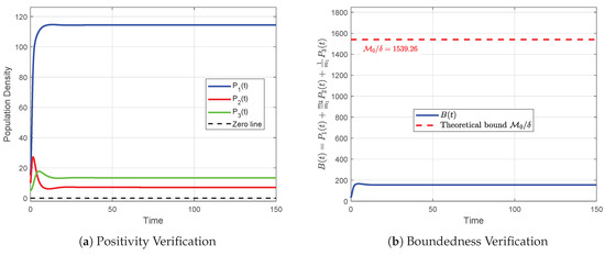
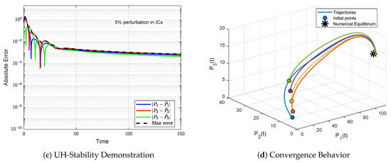
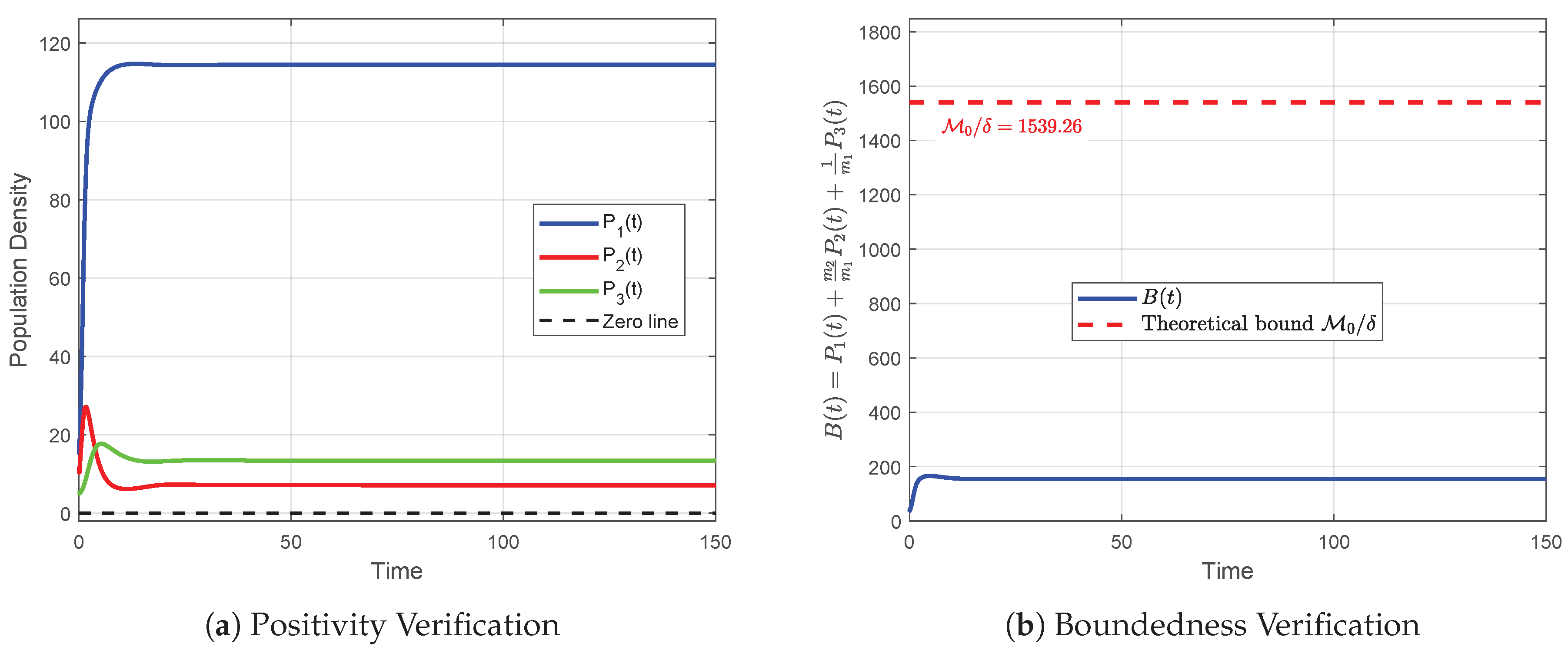
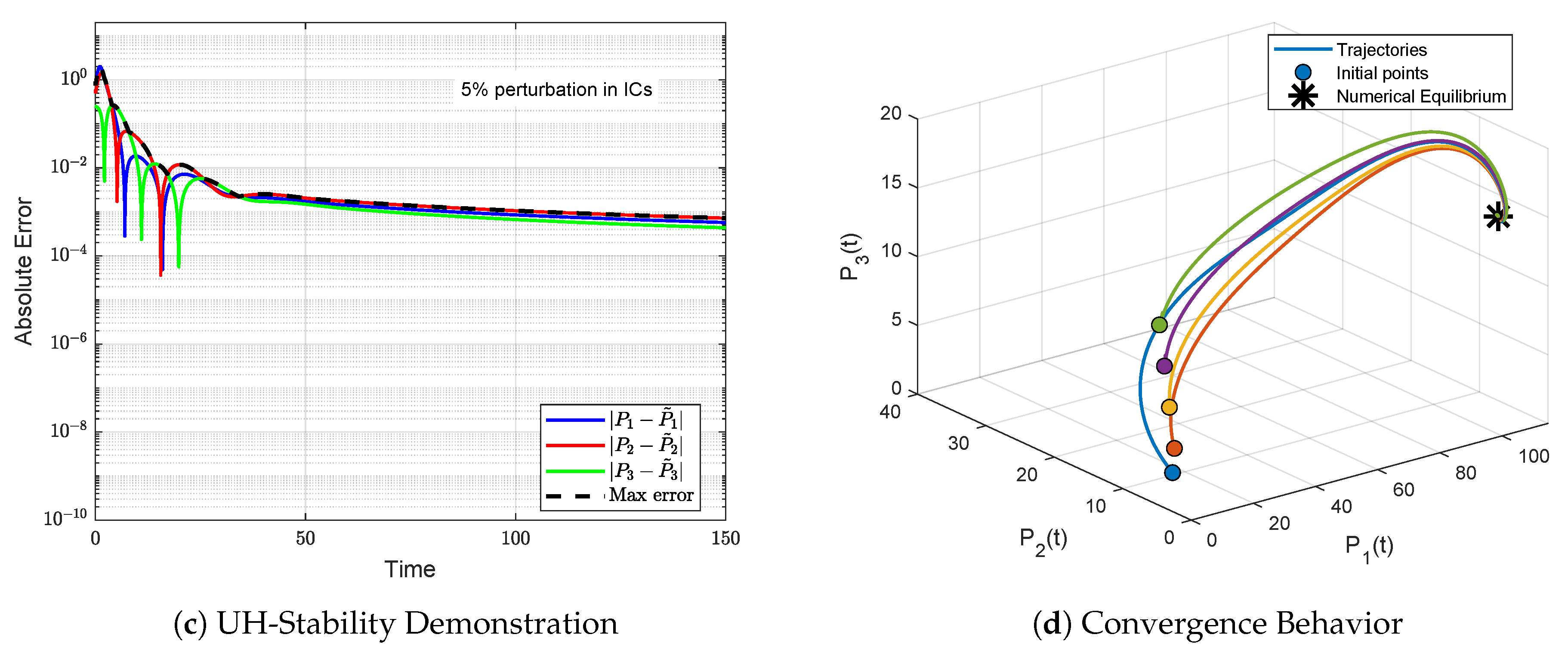
To verify the main analytical properties established in Section 4, numerical simulations are performed over a time horizon of $t\in [0,150]$ with the time step $\Delta t=0.05$ using the baseline fractional order $\varpi =0.95$, the characteristic time-scale $\tau =1$, and the initial population biomasses $P_1\left(0\right)=15$, $P_2\left(0\right)=10$, and $P_3\left(0\right)=5$. The complete baseline parameter values and numerical settings are summarized in Table 2. The corresponding numerical results are presented in Figure 2. Figure 2a shows that all population trajectories remain strictly positive, supporting the non-negativity result of Lemma 3. Figure 2b demonstrates boundedness, with the weighted biomass $Z\left(t\right)=P_1\left(t\right)+{\displaystyle \frac{m_2}{m_1}}{P}_2\left(t\right)+{\displaystyle \frac{1}{m_1}}{P}_3\left(t\right)$ remaining below the analytical threshold ${\mathcal{M}}_0/\delta \approx 1539.26$, consistent with Lemma 4. Figure 2c illustrates the response to a $5\%$ perturbation, with the resulting errors remaining uniformly bounded, providing numerical evidence consistent with the Ulam–Hyers stability estimate in Theorem 2. Finally, Figure 2d shows the trajectories corresponding to five different initial configurations, which converge toward the same stable coexistence state, providing numerical evidence of the observed asymptotic convergence.

Figure 2. Numerical verification of the fundamental analytical properties of the FEEM (7) over a time horizon $[0,150]$.

5.3. Numerical Assessment of Fractional-Order Effects

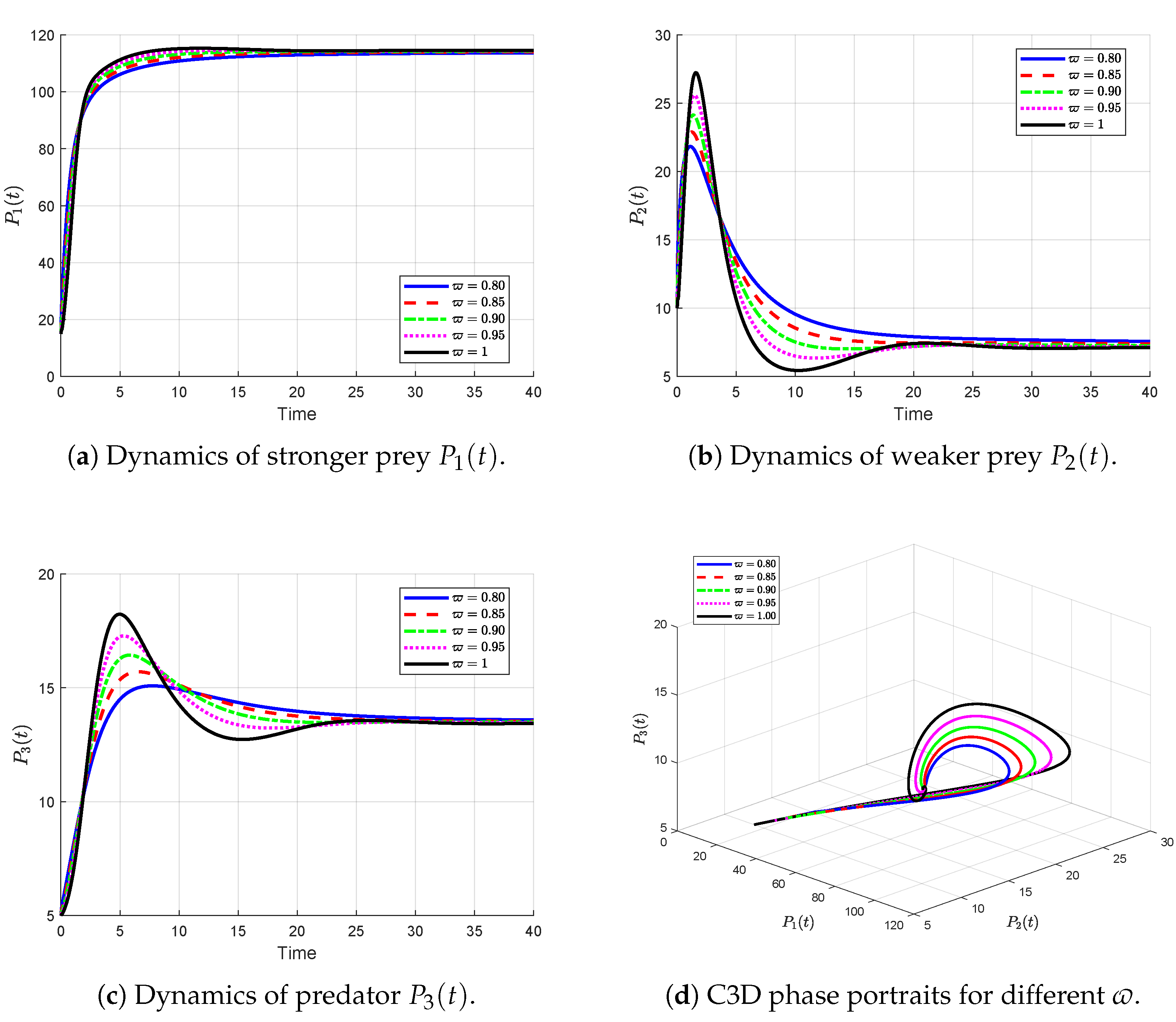
To assess the influence of the fractional order on the transient dynamics of the FEEM (7), numerical simulations are performed for $\varpi \in \{0.80,0.85,0.90,0.95,1.00\}$, while all biological parameters, the initial conditions, the characteristic time-scale $\tau =1$, and the numerical step size are kept unchanged as previously defined. The classical case $\varpi =1$ is included as a reference for comparison with the fractional-order formulations.

Figure 3a shows that the stronger prey $P_1$ exhibits a rapid increase for all tested fractional orders and subsequently approaches a nearly common long-term level. The main effect of decreasing $\varpi$ is observed in the transient regime: the classical case $\varpi =1$ produces the fastest initial growth and the largest transient overshoot, whereas smaller fractional orders lead to a smoother and more gradual approach to the long-term state.

Figure 3. Numerical assessment of the fractional-order effects in the FEEM (7) for $\varpi \in \{0.80,0.85,0.90,0.95,1\}$ over a time horizon $[0,40]$.

A more pronounced fractional-order dependence is observed for the weak prey $P_2$ in Figure 3b. For $\varpi =1$, the population reaches the highest initial peak, followed by a pronounced decline before recovering toward its long-term level. As $\varpi$ decreases, both the initial peak and the depth of the subsequent decline are progressively reduced. Thus, the fractional formulation modifies the amplitude and damping of the transient response while the trajectories remain bounded and approach a similar long-term population level.

The predator population $P_3$, shown in Figure 3c, exhibits a comparable dependence on the fractional order. The classical case produces the largest initial peak and the strongest subsequent oscillatory excursion, whereas decreasing $\varpi$ progressively smooths these transient fluctuations. Nevertheless, all trajectories eventually approach a closely similar long-term level.

The corresponding three-dimensional phase portraits in Figure 3d further illustrate the effect of the fractional order on the transient geometry of the system. The trajectories form transient excursions in the $(P_1,P_2,P_3)$ state space and subsequently contract toward a common terminal region. The classical trajectory ($\varpi =1$) exhibits the largest excursion, while decreasing the fractional order progressively reduces the size of the transient orbit. These results indicate that the fractional order primarily controls the strength and duration of transient population fluctuations, reflecting the influence of hereditary memory, whereas the long-term population levels remain relatively insensitive to the tested fractional orders.

5.4. Numerical Assessment of the Characteristic Time-Scale

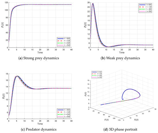
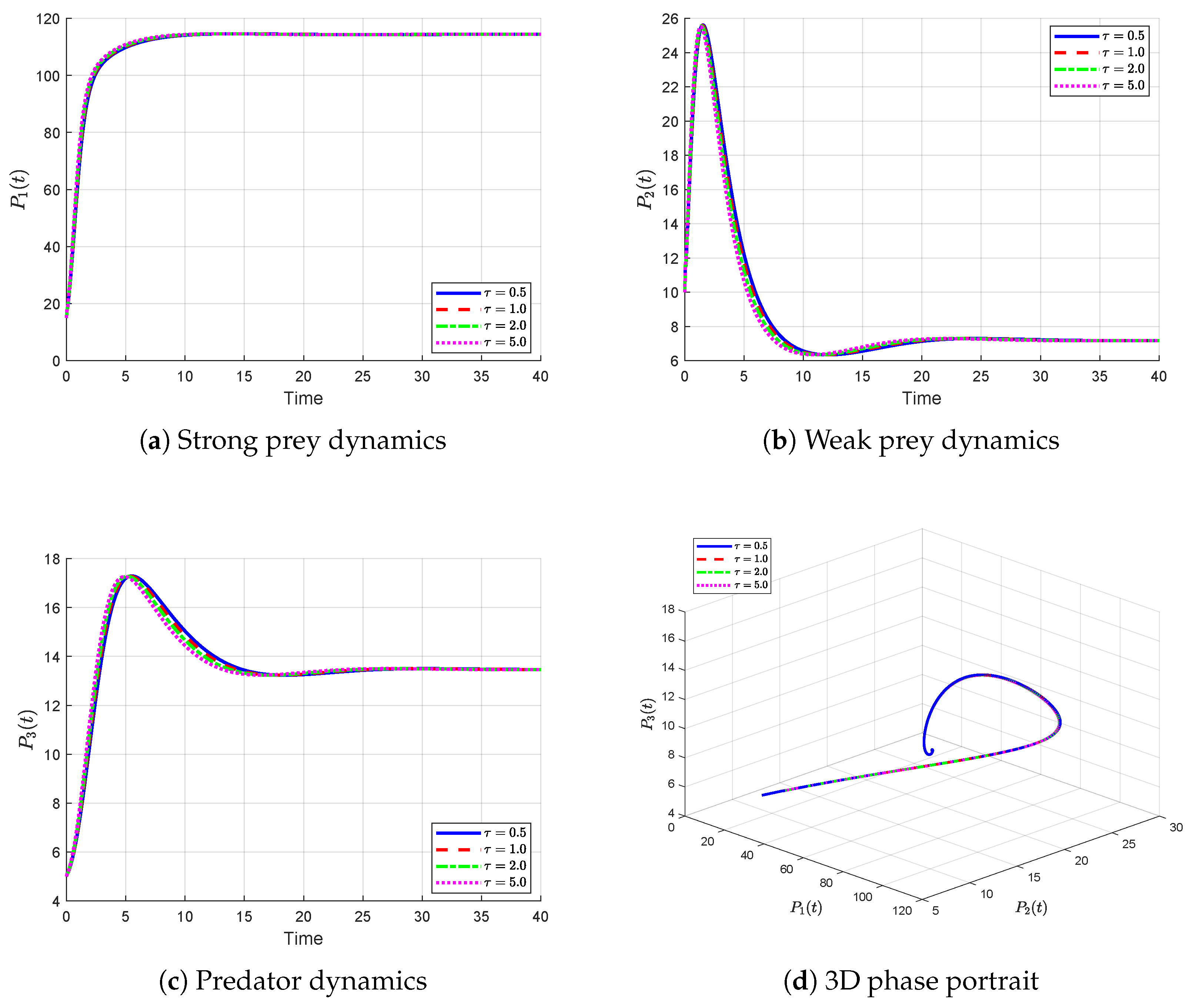
To assess the influence of the characteristic time-scale $\tau$ on the transient dynamics of the FEEM (7), numerical simulations are performed for $\tau \in \{0.5,1.0,2.0,5.0\}$ while keeping the fractional order fixed at $\varpi =0.95$. All biological parameters, numerical settings, and initial conditions are kept unchanged. The effect of $\tau$ is therefore examined independently through the scaling factor ${\tau }^{1-\varpi }$.

Figure 4 illustrates the resulting population dynamics. For the strong prey $P_1\left(t\right)$ (Figure 4a), the trajectories corresponding to the four characteristic time-scales remain close to one another. The population increases from its initial value and approaches a nearly steady level of approximately 110–120, with only minor differences in the transient evolution. This indicates that variations in $\tau$ have a relatively weak effect on the long-term dynamics of the strong prey.

Figure 4. Numerical assessment of the characteristic time-scale for $\tau \in \{0.5,1.0,2.0,5.0\}$ with fixed fractional order $\varpi =0.95$ over $t\in [0,40]$.

For the weak prey $P_2\left(t\right)$ (Figure 4b), the influence of $\tau$ is more apparent during the transient phase. The population initially increases to approximately 25–30, subsequently decreases to a lower level, and then gradually recovers toward a nearly steady value around 7–8. The different values of $\tau$ produce small shifts in the transient trajectory and in the timing of these changes, while the eventual behavior remains similar.

The predator population $P_3\left(t\right)$ exhibits a comparable response (Figure 4c). The trajectories initially increase to approximately 18, followed by a decline toward a level near 13–14, after which the solutions approach a nearly steady state. The differences between the characteristic time-scales are mainly observed during the transient stage rather than in the asymptotic behavior.

The corresponding three-dimensional phase portrait is presented in Figure 4d. The trajectories associated with the different values of $\tau$ remain close and approach the same region of the phase space. Thus, within the considered parameter regime, the characteristic time-scale primarily modifies the transient pathway of the ecological system, whereas its long-term dynamical behavior remains essentially unchanged. This observation is consistent with the role of ${\tau }^{1-\varpi }$ as a scaling factor in the fractional formulation.

5.5. Numerical Sensitivity Analysis of the Strong Allee Effect

To assess the influence of the strong Allee effect on the dynamics of the FEEM (7), numerical simulations are performed by varying the parameters $C_1$ and $C_2$ appearing in the Allee-modified growth term of the stronger prey population $P_1$. All remaining biological parameters and numerical settings are kept at their baseline values, with fractional order $\varpi =0.95$, characteristic time-scale $\tau =1$, and initial conditions $P_1\left(0\right)=15, P_2\left(0\right)=10$, and $P_3\left(0\right)=5$.

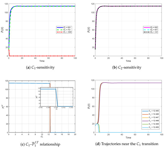
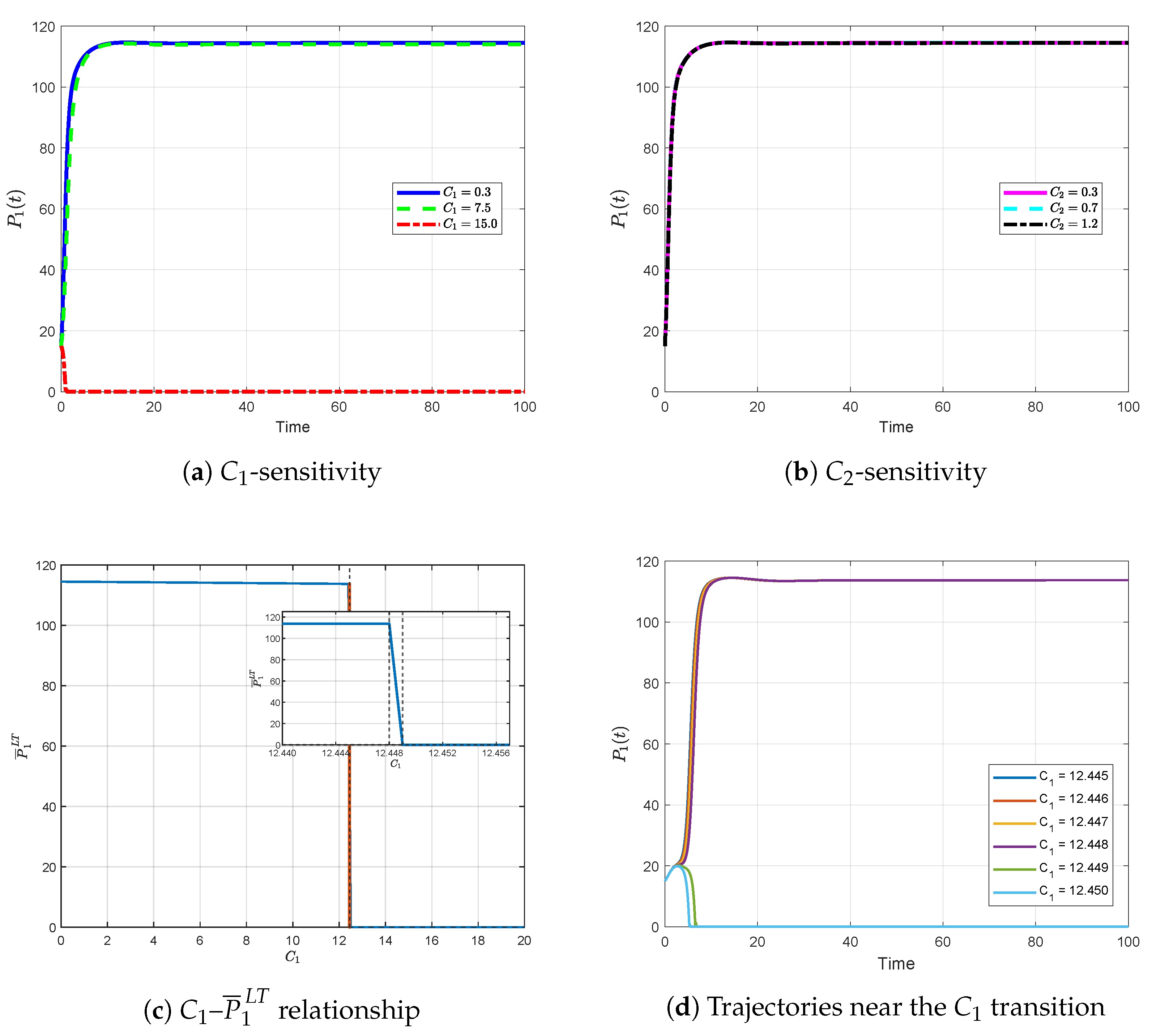
Figure 5 illustrates the resulting sensitivity of the stronger prey population to the two Allee-effect parameters. For the Allee-threshold parameter $C_1$ (Figure 5a), the trajectories corresponding to $C_1=0.3$ and $C_1=7.5$ persist and approach a nearly steady level of approximately $P_1\approx 115$. In contrast, for $C_1=15$, the population rapidly declines toward zero. This pronounced difference indicates that $C_1$ plays a dominant role in determining whether the stronger prey persists or becomes extinct under the considered parameter regime.

Figure 5. Numerical sensitivity analysis of the strong Allee effect on the stronger prey population $P_1$ for fixed fractional order $\varpi =0.95$, characteristic time-scale $\tau =1$, and initial conditions $P_1\left(0\right)=15$, $P_2\left(0\right)=10$, and $P_3\left(0\right)=5$.

For the auxiliary Allee parameter $C_2$ (Figure 5b), the trajectories corresponding to $C_2\in \{0.3,0.7,1.2\}$ remain close and converge toward nearly the same long-term population level. Thus, within the investigated range, variations in $C_2$ have a considerably weaker effect on the dynamics of $P_1$ than variations in $C_1$. This behavior is consistent with the structure of the Allee correction ${\displaystyle \frac{P_1-C_1}{P_1+C_2}},$ where $C_1$ determines the zero of the Allee factor, whereas $C_2$ primarily modifies its density-dependent scaling.

To identify the persistence and extinction transition associated with $C_1$ more systematically, $C_1$ is subsequently varied over the interval $0\le C_1\le 20$, while $C_2=0.7$ is held fixed. For each value of $C_1$, the long-term response of the stronger prey is characterized by the mean population over the final $10\%$ of the simulation interval, ${\overline{P}}_1^{LT}={\displaystyle \frac{1}{N_{LT}}}{\sum }_{j\in {\mathcal{I}}_{LT}}{P}_1\left(t_j\right),$ where ${\mathcal{I}}_{LT}$ denotes the set of time indices corresponding to the final $10\%$ of the simulation. Numerical extinction is classified according to the criterion ${\overline{P}}_1^{LT}\le {10}^{-3}.$ A coarse sweep with increment $\Delta C_1=0.1$ is first employed to locate the transition region, followed by a refined sweep with increment $\Delta C_1=0.001$.

The resulting $C_1$–${\overline{P}}_1^{LT}$ relationship is presented in Figure 5c. The long-term stronger prey population remains on a high-persistence branch over most of the investigated range and then undergoes an abrupt collapse within a narrow interval of $C_1$. The inset provides an enlarged view of this transition region. The refined computation identifies $C_1=12.448$ as the last tested value for which the stronger prey persists, whereas $C_1=12.449$ is the first tested value satisfying the numerical extinction criterion. Accordingly, for the selected parameter set, initial conditions, simulation horizon, and extinction criterion, the numerical persistence and extinction transition is bracketed by

$$12.448<C_{1,\mathrm{tr}}<12.449.$$

The sharp transition observed in Figure 5c is further examined through the fine-resolution time-domain trajectories shown in Figure 5d. For

$$C_1\in \{12.445,12.446,12.447,12.448,12.449,12.450\},$$

the trajectories exhibit two distinctly different long-term outcomes. For $C_1=12.445$, $12.446$, $12.447$, and $12.448$, the stronger prey initially undergoes a transient response and subsequently recovers toward the persistent state near $P_1\approx 114$. In contrast, for $C_1=12.449$ and $C_1=12.450$, the population decreases to zero after a short transient. These trajectories therefore corroborate the transition identified from the systematic $C_1$–${\overline{P}}_1^{LT}$ analysis.

Overall, the numerical results demonstrate a markedly stronger sensitivity of the stronger prey dynamics to $C_1$ than to $C_2$. In particular, under the prescribed initial condition $P_1\left(0\right)=15$ and the selected baseline parameter set, a small increase in $C_1$ across the narrow interval between $12.448$ and $12.449$ changes the long-term outcome from persistence to numerical extinction. The reported interval should therefore be interpreted as a numerical persistence and extinction transition for the specified simulation conditions.

5.6. Sensitivity Analysis of Anthropogenic Harvesting

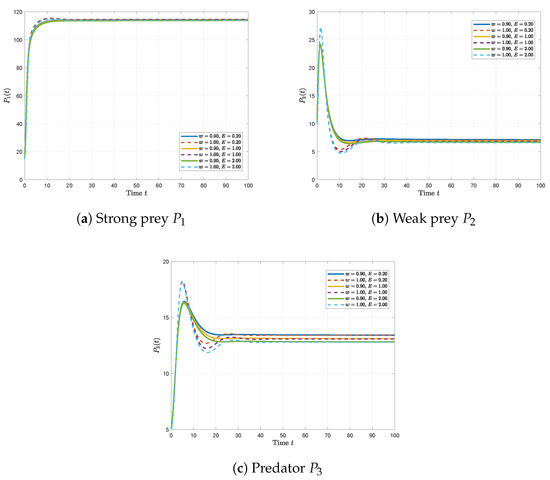
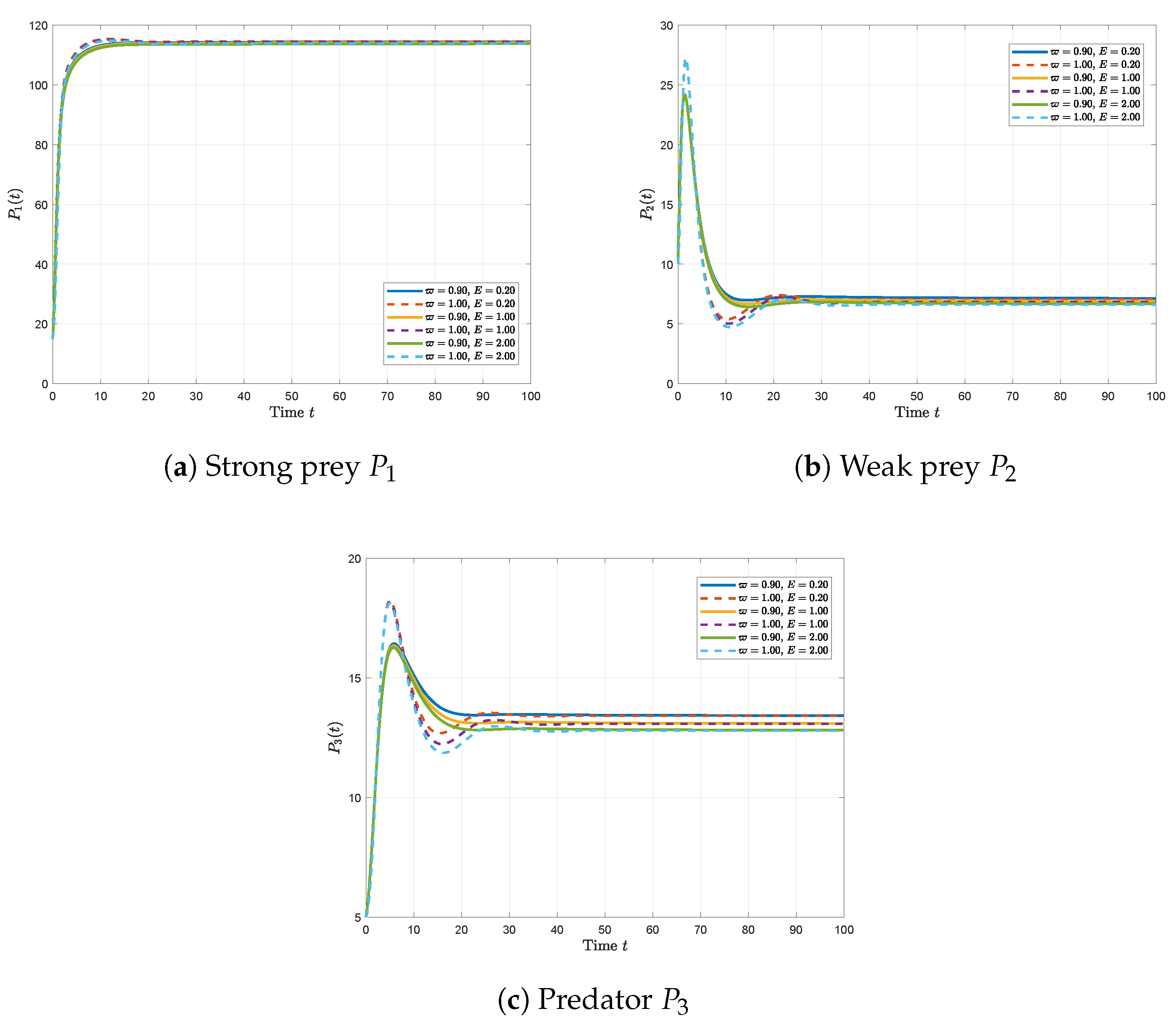
To assess the temporal response of the FEEM to anthropogenic exploitation, we consider three representative harvesting effort levels, $E\in \{0.20,1.00,2.00\}$, with the same baseline parameter values adopted in the preceding numerical experiments. The harvesting effort is applied equally to both prey populations, i.e., $E_1=E_2=E$. The fractional-order model with $\varpi =0.90$ is compared with the corresponding classical integer-order model obtained by setting $\varpi =1.00$, while the characteristic time-scale parameter is kept fixed at $\tau =1$.

Figure 6 summarizes the responses of the three populations under the selected harvesting intensities. For the strong prey $P_1$, increasing the harvesting effort produces a clear reduction in population density and modifies its temporal trajectory. The comparison between $\varpi =0.90$ and $\varpi =1.00$ indicates that the fractional model exhibits a different temporal response due to the incorporation of memory effects. Thus, the harvesting impact is not determined solely by the instantaneous removal term, but is also influenced by the memory-dependent dynamics of the system.

Figure 6. Temporal responses of the strong prey $P_1$, weak prey $P_2$, and predator $P_3$ under selected harvesting efforts $E\in \{0.20,1.00,2.00\}$, comparing the fractional-order model ($\varpi =0.90$) with the classical integer-order model ($\varpi =1.00$).

A similar response is observed for the weak prey $P_2$. As the harvesting effort increases, the population is increasingly suppressed. The difference between the fractional and classical trajectories becomes evident in their transient behavior, reflecting the fact that the fractional formulation retains information from the previous states of the population. Consequently, the response to harvesting is distributed over the temporal history of the system rather than being determined exclusively by its instantaneous state.

The predator population $P_3$ exhibits an indirect response to harvesting. Since harvesting is applied directly to the prey populations, its effect on the predator is transmitted through the trophic interactions. Increasing E reduces the availability of prey and consequently alters the temporal dynamics of the predator population. The comparison between $\varpi =0.90$ and $\varpi =1.00$ further demonstrates that the memory effect influences this bottom-up response, although the magnitude of the predator response depends on the strength of the prey–predator interactions.

6. Conclusions and Future Work

In this study, we developed and analyzed a fractional Lotka–Volterra predator–prey model incorporating a strong Allee effect, nonlinear anthropogenic harvesting, and memory-dependent dynamics through the Atangana–Baleanu–Caputo (ABC) fractional operator. The theoretical analysis established the existence and uniqueness, non-negativity, ultimate boundedness, and Ulam–Hyers stability of the system under the stated assumptions. Numerical investigations showed that the fractional order $\varpi$ modifies the temporal dynamics of the interacting populations, highlighting the influence of memory, while the characteristic time-scale $\tau$ regulates the fractional response through the factor ${\tau }^{1-\varpi }$.

The sensitivity analysis of the strong Allee effect showed that the threshold parameter $C_1$ plays a critical role in the persistence of the stronger prey. For the prescribed initial conditions $P_1\left(0\right)=15$, $P_2\left(0\right)=10$, and $P_3\left(0\right)=5$ and the selected parameter set, the systematic $C_1$–${\overline{P}}_1^{LT}$ analysis identified $C_1=12.448$ as the last persistent tested value and $C_1=12.449$ as the first numerically extinct tested value, bracketing the numerical persistence and extinction transition within $12.448<C_{1,\mathrm{tr}}<12.449$. In contrast, variations in the auxiliary Allee parameter $C_2$ produced a substantially less pronounced effect over the investigated range.

The harvesting simulations further showed that increasing anthropogenic exploitation modifies the dynamics of both prey populations and consequently affects the predator through trophic interactions, while fractional memory alters the temporal response to harvesting. Overall, the results demonstrate the importance of Allee effects, harvesting pressure, and fractional memory in shaping the dynamics of the proposed predator–prey system. Future work will investigate the effects of $\varpi$ and $\tau$ on equilibrium stability and conduct a systematic bifurcation analysis to identify critical parameter values and transitions between different dynamical regimes.

References

- Aguirre, P.; Flores, J.D.; González-Olivares, E. Bifurcations and global dynamics in a predator–prey model with a strong Allee effect on the prey, and a ratio-dependent functional response. Nonlinear Anal. Real World Appl. 2014, 16, 235–249. [Google Scholar] [CrossRef] [Scilit]
- Thirthar, A.A.; Panja, P.; Majeed, S.J.; Nisar, K.S. Dynamic interactions in a two-species model of the mammalian predator–prey system: The influence of Allee effects, prey refuge, water resources, and moonlights. Partial Differ. Equ. Appl. Math. 2024, 11, 100865. [Google Scholar] [CrossRef] [Scilit]
- Yaseen, R.M.; Helal, M.M.; Dehingia, K.; Mohsen, A.A. Effect of the fear factor and prey refuge in an asymmetric predator–prey model. Braz. J. Phys. 2024, 54, 214. [Google Scholar] [CrossRef] [Scilit]
- Dasumani, M.; Lassong, B.S.; Akgül, A.; Osman, S.; Moore, S.E. Analyzing the dynamics of human papillomavirus transmission via fractal and fractional dimensions under Mittag–Leffler Law. Model. Earth Syst. Environ. 2024, 10, 7225–7249. [Google Scholar] [CrossRef] [Scilit]
- Youssef, M.I.; Dasumani, M.; Maina, R.M.; Radwan, A.; Gathungu, D.K. An Atangana–Baleanu fractional derivative approach to modeling diabetes progression and optimizing comorbidity reduction and prevention. Fractal Fract. 2025, 9, 820. [Google Scholar] [CrossRef] [Scilit]
- Zakirullah; Lu, C.; Li, L.; Shah, K.; Abdalla, B.A.; Abdeljawad, T. Mathematical insights into chaos in fractional-order fishery model. Model. Earth Syst. Environ. 2025, 11, 201. [Google Scholar] [CrossRef] [Scilit]
- Ramesh, K.; Kumar, G.R.; Nisar, K.S. A nonlinear mathematical model on the dynamical study of a fractional-order delayed predator–prey scheme that incorporates harvesting together and Holling type-II functional response. Results Appl. Math. 2023, 19, 100390. [Google Scholar] [CrossRef] [Scilit]
- Ramesh, K.; Kumar, G.R.; Khan, A.; Abdeljawad, T. Analysis of the stability of a predator–prey model including the memory effect, double Allee effect and Holling type-I functional response. PLoS ONE 2025, 20, e0305179. [Google Scholar] [CrossRef] [Scilit]
- Kalra, P.; Malhotra, N. Dynamical and numerical analysis of a fractional order three species food chain model with Holling type II functional response and Allee effect. J. Math. Sci. 2026, 298, 58–79. [Google Scholar] [CrossRef] [Scilit]
- Kumar, G.R.; Ramesh, K.; Khan, A.; Lakshminarayan, K.; Abdeljawad, T. Bazykin’s predator–prey model includes a dynamical analysis of a Caputo fractional order delay fear and the effect of the population-based mortality rate on the growth of predators. Qual. Theory Dyn. Syst. 2024, 23, 130. [Google Scholar] [CrossRef] [Scilit]
- Vijayalakshmi, G.M.; Nisar, K.S.; Reddy, K.S. Mittag–Leffler kernel operator on prey–predator model interfusing intra-specific competition and prey fear factor. Partial Differ. Equ. Appl. Math. 2024, 9, 100637. [Google Scholar] [CrossRef] [Scilit]
- Kumar, S.; Singh, R.; Chauhan, R.P.; Thakur, N.K. Investigation of an interacting fractional-order predator–prey system in presence of fear and harvesting. Iran. J. Sci. 2023, 47, 1739–1749. [Google Scholar] [CrossRef] [Scilit]
- Anggriani, N.; Panigoro, H.S.; Rahmi, E.; Peter, O.J.; Jose, S.A. A predator–prey model with additive Allee effect and intraspecific competition on predator involving Atangana–Baleanu–Caputo derivative. Results Phys. 2023, 49, 106489. [Google Scholar] [CrossRef] [Scilit]
- Jana, S.; Ghorai, A.; Guria, S.; Kar, T.K. Global dynamics of a predator, weaker prey and stronger prey system. Appl. Math. Comput. 2015, 250, 235–248. [Google Scholar] [CrossRef] [Scilit]
- Singh, A.; Malik, P. Bifurcations in a modified Leslie–Gower predator–prey discrete model with Michaelis–Menten prey harvesting. J. Appl. Math. Comput. 2021, 67, 143–174. [Google Scholar] [CrossRef] [Scilit]
- Krishna, S.V.; Srinivasu, P.D.N.; Kaymakcalan, B. Conservation of an ecosystem through optimal taxation. Bull. Math. Biol. 1998, 60, 569–584. [Google Scholar] [CrossRef] [Scilit]
- Clark, C.W. Mathematical models in the economics of renewable resources. SIAM Rev. 1979, 21, 81–99. [Google Scholar] [CrossRef] [Scilit]
- Arancibia-Ibarra, C.; Flores, J.; Bode, M.; Pettet, G.; van Heijster, P. A modified May–Holling–Tanner predator–prey model with multiple Allee effects on the prey and an alternative food source for the predator. Discret. Contin. Dyn. Syst. B 2021, 26, 943–962. [Google Scholar] [CrossRef] [Scilit]
- Berec, L.; Angulo, E.; Courchamp, F. Multiple Allee effects and population management. Trends Ecol. Evol. 2007, 22, 185–191. [Google Scholar] [CrossRef] [Scilit]
- Ghosh, B.; Kar, T.K. Sustainable use of prey species in a prey–predator system: Jointly determined ecological thresholds and economic trade-offs. Ecol. Model. 2014, 272, 49–58. [Google Scholar] [CrossRef] [Scilit]
- Podlubny, I. Fractional Differential Equations: An Introduction to Fractional Derivatives, Fractional Differential Equations, to Methods of Their Solution and Some of Their Applications; Academic Press: San Diego, CA, USA, 1998; Volume 198. [Google Scholar]
- Kumar, S.; Chauhan, R.P.; Aly, A.A.; Momani, S.; Hadid, S. A study on fractional HBV model through singular and non-singular derivatives. Eur. Phys. J. Spec. Top. 2022, 231, 1885–1904. [Google Scholar] [CrossRef] [Scilit]
- Atangana, A.; Baleanu, D. New fractional derivatives with non-local and non-singular kernel: Theory and application to heat transfer model. Therm. Sci. 2016, 20, 763–769. [Google Scholar] [CrossRef] [Scilit]
- Lassong, B.S.; Dasumani, M.; Mung’atu, J.K.; Moore, S.E. Power and Mittag–Leffler laws for examining the dynamics of fractional unemployment model: A comparative analysis. Chaos Solitons Fractals X 2024, 13, 100117. [Google Scholar] [CrossRef] [Scilit]
- Mursaleen, M.; Ansari, K.J. On the stability of some positive linear operators from approximation theory. Bull. Math. Sci. 2015, 5, 147–157. [Google Scholar] [CrossRef] [Scilit]
- Al-Refai, M. Maximum principles and applications for fractional differential equations with operators involving Mittag–Leffler function. Fract. Calc. Appl. Anal. 2021, 24, 1220–1230. [Google Scholar] [CrossRef] [Scilit]
- Atangana, A.; Qureshi, S. Modeling attractors of chaotic dynamical systems with fractal–fractional operators. Chaos Solitons Fractals 2019, 123, 320–337. [Google Scholar] [CrossRef] [Scilit]
Disclaimer/Publisher’s Note: The statements, opinions and data contained in all publications are solely those of the individual author(s) and contributor(s) and not of MDPI and/or the editor(s). MDPI and/or the editor(s) disclaim responsibility for any injury to people or property resulting from any ideas, methods, instructions or products referred to in the content. |
© 2026 by the authors. Licensee MDPI, Basel, Switzerland. This article is an open access article distributed under the terms and conditions of the Creative Commons Attribution (CC BY) license.