Federated Learning with Multi-Method Adaptive Aggregation for Enhanced Defect Detection in Power Systems

Abstract

The detection and identification of defects in transmission lines using computer vision techniques is essential for maintaining the safety and reliability of power supply systems. However, existing training methods for transmission line defect detection models predominantly rely on single-node training, potentially limiting the enhancement of detection accuracy. To tackle this issue, this paper proposes a server-side adaptive parameter aggregation algorithm based on multi-method fusion (SAPAA-MMF) and formulates the corresponding objective function. Within the federated learning framework proposed in this paper, each client executes distributed synchronous training in alignment with the fundamental process of federated learning. The hierarchical difference between the global model, aggregated using the improved joint mean algorithm, and the global model from the previous iteration is computed and utilized as the pseudo-gradient for the adaptive aggregation algorithm. This enables the adaptive aggregation to produce a new global model with improved performance. To evaluate the potential of SAPAA-MMF, comprehensive experiments were conducted on five datasets, involving comparisons with several algorithms. The experimental results are analyzed independently for both the server and client sides. The findings indicate that SAPAA-MMF outperforms existing federated learning algorithms on both the server and client sides.

1. Introduction

Ensuring a stable power supply through the power grid is a crucial factor in maintaining quality of life and the seamless functioning of society. Timely detection of faults and defects in transmission lines is essential for maintaining the stability of power system operations. Consequently, transmission line defect detection has emerged as a research hotspot, garnering significant attention from both academia and the power industry, and has been extensively studied by numerous scholars.

In recent years, the rapid advancement of deep learning has prompted researchers to employ it for object detection, leading to the development of numerous deep learning-based object detection algorithms. For insulator defect detection, Miao et al. [1] employed transfer learning strategies, utilizing the COCO (Common Objects in Context) pre-trained model for domain adaptation to construct a Single Shot MultiBox Detector (SSD) model that incorporates various insulator types using diverse backgrounds. Zhao et al. [2] proposed an improved insulator detection method based on Faster R-CNN, fine-tuning the model and introducing an enhanced anchor box generation technique to improve detection precision and significantly enhance performance in handling occlusion. Feng et al. [3] introduced an automatic insulator detection approach utilizing the YOLOv5x object detection model in combination with the K-means algorithm. This approach optimizes model performance, facilitating the rapid and accurate detection and localization of targets in images. For detecting foreign objects in bird nests, Ju et al. [4] proposed a real-time bird nest detection approach leveraging the spatial relationship between bird nests and tower poles. This approach employs SSD as the detector and utilizes deep neural networks to establish the spatial relationship between tower poles and bird nests. By leveraging tower pole detection results to refine bird nest detection, this approach enhances both the accuracy and efficiency of bird nest identification.

Although the aforementioned detection models have achieved considerable success in identifying defects in transmission lines, their training methodologies primarily rely on single-node systems. Training defect detection models on a single node restricts effective data sharing and connectivity, hindering comprehensive integration and analysis of data from diverse environments. This, in turn, affects the diversity and generalization capabilities of transmission line defect detection models. Furthermore, single-node training raises concerns regarding privacy security and the inability to handle large-scale data [5]. In 2016, Google Research introduced the concept of federated learning to enhance privacy protection and address the challenge of data silos [6]. The primary goal of federated learning is to enable model training without centrally storing or transmitting raw data. Due to its superior performance and enhanced security compared to traditional distributed machine learning, federated learning has rapidly become a prominent paradigm in the field [7]. Hong et al. [8] proposed a joint adversarial debiasing method that allows users to opt out of the debiasing session based on privacy or computational cost concerns without accessing sensitive group information. This method addresses the issue of model bias and unfairness arising from the heterogeneity of user data in federated learning. Karimireddy et al. [9] proposed the stochastic control averaging algorithm, which utilizes control variables to reduce drift between clients during local updates, thereby addressing the issues of unstable and slow model convergence. Yuan et al. [10] proposed the joint pairwise averaging algorithm, which overcomes the limitations of traditional averaging by introducing an innovative server-side pairwise averaging procedure. This approach effectively improves convergence speed and optimization in federated learning tasks involving non-smooth regularization terms. Traditional federated learning algorithms have achieved progress by optimizing parameter aggregation and improving communication efficiency, but the aggregated global model continues to suffer from poor performance and generalization. Most traditional federated learning algorithms optimize parameter aggregation from a single perspective, overlooking the complementary advantages of integrating different algorithms, which limits model performance.

To tackle these challenges, this paper introduces a Server-side Adaptive Parameter Aggregation Algorithm Based on Multi-method Fusion (SAPAA-MMF). This approach takes into account data silos, privacy security, and hardware performance issues inherent in defect detection tasks dependent on single-node training models. The study constructs a transmission line defect detection network utilizing the single-stage object detection algorithm SSD as the client model for local training within a federated learning framework. By leveraging the complementarity of algorithms, the adaptive aggregation algorithm FedAdam [11] serves as the base algorithm, which is combined with the improved federated averaging algorithm FedAvg [11] to enhance server-side parameter aggregation in federated learning. This approach yields a more effective global model.

• The SAPAA-MMF method integrates various algorithms by utilizing the average model variance as the pseudo-gradient for adaptive aggregation. This approach addresses the limitations of previous single-parameter aggregation algorithms, which often struggled to ensure both the convergence and stability of the global model. By leveraging the average model variance, SAPAA-MMF enables a more robust and stable parameter aggregation process, resulting in enhanced performance and generalization of the global model in federated learning scenarios.
• In this paper, we propose a weight balancing method that comprehensively considers factors such as client-side local data distribution and data quality in the aggregation process. This method ensures that different training nodes or devices can contribute effectively to the global model, thereby maximizing the advantages of various algorithms. By accounting for the variability in local data and the quality of client contributions, the weight balancing method improves the aggregation process, resulting in a more accurate and robust global model in federated learning.
• The SAPAA-MMF method proposed in this paper significantly improves defect detection in transmission lines. Extensive experiments against several state-of-the-art methods demonstrate the effectiveness and superiority of SAPAA-MMF. The results indicate that SAPAA-MMF outperforms existing methods by providing more accurate and reliable defect detection, thereby confirming its potential and advantages in practical applications.

2. Related Work

2.1. Defect Detection

In the traditional field of image processing research, researchers mainly use artificially designed feature extraction algorithms to build models for visual characteristics such as color and morphological edges, aiming to effectively distinguish key objects from complex background environments, performing various defect detection tasks accordingly. Wu et al. [12] proposed a new active contour model, which uses a semi-local operator to extract texture features, defines a new function to handle texture inhomogeneity, and uses a fast dual form to make contour evolution more efficient. The model can extract uneven insulators from aerial images and overcome the recognition difficulties caused by texture inhomogeneity. Using only a single feature cannot significantly improve the detection effect. Therefore, Wang et al. [13] proposed a recognition method that integrates the shape, color, and texture information of insulators. First, parallel line features are perceived from different directions as candidate features of the insulators. Then, the candidate region is expanded and semantic analysis is performed using local binary patterns to identify the insulator region. Finally, the main color component analysis is used to compensate for the insulator region, the region is adaptively divided according to the average distance, the texture feature changes are analyzed, and the insulator shedding defect is detected. Considering that image noise can also affect the detection results, Yan et al. [14] proposed a maximum inter-class variance algorithm based on morphological methods, designed a new filtering method to remove tiny noise according to the characteristics of power lines, and successfully identified the redundant materials on the power lines by comparing the number of local maxima in the measured power lines and Hough transfer accumulators through the Hough transform feature. Chen et al. [15] addressed the limitations of traditional pavement defect detection methods by proposing MANet, a multi-scale mobile attention-based network that integrates multi-scale convolutions and hybrid attention mechanisms to enhance feature extraction and improve the accuracy of pavement defect detection. Yu et al. [16] addressed the limitations of using methods like graph convolutional networks (GCN) by constructing high-quality graphs with multi-source sensors and utilizing a two-stage framework for fault diagnosis, thereby enhancing the robustness of fault diagnosis.

Although the above algorithms have achieved some results, they have limitations in feature acquisition and real-time performance, which limits the accuracy and efficiency of detection. In recent years, with the rapid development of deep learning [17], researchers have adopted deep learning for target detection, and many deep learning-based target detection algorithms have emerged. The target detection algorithm based on deep learning has achieved good results in image feature extraction and complex and diverse image features. This type of algorithm can automatically identify the features in an image and overcomes the shortcomings of traditional algorithms. In insulator defect detection, Miao et al. [1] borrowed the transfer learning strategy, made domain adaptability adjustments through the COCO (Common Objects in Context) pre-trained model, and constructed an SSD (Single Shot MultiBox Detector) detection model that includes multiple insulator types using multivariate backgrounds. On this basis, the initial model is fine-tuned using training data from specific insulator samples and their complex application scenarios to accurately identify insulators. Zhao et al. [2] proposed an insulator detection method based on an improved Faster R-CNN. By fine-tuning the Faster R-CNN model and using an improved anchor box generation method, the accuracy of insulator detection is improved while significant improvements are made in handling occlusion. Feng et al. [3] proposed an automatic insulator detection method based on the YOLOv5x target detection model. This method combines the YOLOv5x model and the K-Means algorithm to achieve the purpose of automatically identifying insulator defects. The performance of the model is optimized by K-means clustering. The YOLOv5x model can quickly and accurately detect and locate targets in the image. In the defect detection of bird nest foreign bodies, Ju et al. [4] proposed a real-time bird nest detection method based on the relationship with the tower pole. This method uses SSD as a detector, uses a deep neural network to establish the relationship between the tower pole and the bird nest, and uses the tower pole detection results to correct the bird nest detection effect, thereby improving the accuracy and efficiency of bird nest detection. Li et al. [18] proposed an automatic detection method for bird nests in power transmission lines based on Faster R-CNN. By magnifying the bird nest image, it not only solves the problem of insufficient training samples and overfitting of the neural network classifier, but also has a good bird nest target detection effect in complex environments. Li et al. [19] addressed the limitations of traditional PV panel defect detection methods by incorporating Ghost convolution with BottleneckCSP and a tiny target prediction head into YOLOv5, significantly enhancing detection accuracy and speed for multiscale PV panel defects. Wang et al. [20] addressed the limitations of traditional road defect detection methods by enhancing YOLOv8 with BiFPN and LSK-attention mechanisms, improving both detection accuracy and model efficiency for real-time applications.

Although the aforementioned detection models have achieved good results in identifying defects in transmission lines, their training methods are primarily based on single nodes. However, in practical applications, transmission lines are widely distributed, and defect data is dispersed across equipment or systems in different regions. The single-node training method for defect detection models leads to a lack of effective sharing and connection between data, preventing comprehensive integration and analysis of data from different environments, thus affecting the data diversity and generalization ability of transmission line defect detection models. Additionally, there are issues related to privacy security and the inability to train large-scale data on a single node.

2.2. Federated Learning

The goal of federated learning is to build a global model by aggregating local updates from multiple clients to adapt to the overall data distribution. The client shares global model parameters with other clients during local training, and the server aggregates local updates to form a global model.

McMahan et al. [6] were the first to propose the concept of federated learning. In response to the needs of massive data training and privacy and security protection, they advocated distributing training data to mobile devices and using local calculated updates for shared model learning. They proposed a practical method for deep network federated learning based on the average iteration model, and the global model was obtained by calculating the mean of the parameters. Blanchard et al. [21] proposed the Krum aggregation algorithm, the core idea of which is to judge the abnormal behavior of nodes based on the similarity between weights, identify abnormal nodes by calculating the distance between weights, and exclude these abnormal nodes to obtain a reliable aggregation result. Yin et al. [22] proposed a robust distributed gradient descent algorithm based on median and truncated mean operations, which enables the algorithm to better solve the Byzantine problem [22] and has good robustness. Pan et al. [23] started by reducing the frequency of federated learning communication, and optimized the balance between local updates and global parameter aggregation by intelligently selecting the number of local updates from the client, thereby reducing the communication frequency between the client and the server. Li et al. [24] added a proximal term to the loss function of the client model to penalize any client model that deviates too much from the global model, so as to prevent the client model from deviating too much from the global model and ensure the convergence of the global model. Li et al. [25] proposed model contrast federated learning by using improved cross entropy loss to perform local optimization and solve the inconsistency problem between foreground and background and by using the similarity between model representations to correct the local training of each party. Zhu et al. [26] proposed a data-free knowledge distillation method to solve heterogeneous federated learning. This method integrates client information without using actual data by training a lightweight generator on the server side and then broadcasting it to the client, adjusting the client’s training process. Reddi et al. [11] proposed an adaptively optimized federated learning algorithm, combined with an adaptive optimization strategy, to achieve effective learning and optimization of the global model on the server side, thereby improving the performance of federated learning. Fallah et al. [27] proposed combining federated learning algorithms with a model-agnostic meta-learning framework. In this approach, models are initialized via meta-learning, and clients perform one or more gradient descent steps on their local datasets to adapt the models. This method retains the advantages of the federated learning architecture while providing more personalized models for each client. Li et al. [28] proposed a private model inheritance scheme that fuses a client’s historical personalized models to guide the subsequent personalized adaptation of the global model, effectively leveraging prior personalized results. Chen et al. [29] proposed a trunk patch-based federated learning architecture, where the shared trunk refines the common knowledge of all participants, and the private patch serves as a compact and efficient module to retain each participant’s domain-specific information, thereby improving model performance. Niu et al. [30] proposed an activation function-based regularizer to correct the gradient of category embeddings by accurately injecting cross-client gradient terms, starting from backpropagation for gradient correction. Collins et al. [31] proposed shared feature representations with local head learning algorithms, which utilize the computational power of distributed clients to perform multiple rounds of local low-dimensional parameter updates. This approach addresses the issues of learning inefficiency and limited model generalization caused by data heterogeneity in federated learning. Shen et al. [32] proposed a novel federated learning paradigm called joint mutual learning to address the issue of data heterogeneity. This paradigm allows each client to independently train personalized models and obtain local models for similar but distinct tasks through collaborative training. Additionally, it enables clients to design customized models for different scenarios and tasks. Shi et al. [33] investigated the challenge of balancing generalization and personalization in blended learning and proposed the personalized joint upper confidence bound algorithm. This algorithm optimally selects the exploration length to balance learning a local model with providing global information for the blended learning objective.

The federated learning algorithm has made some achievements in terms of parameter aggregation effect and communication efficiency, but the aggregated global model still has problems such as poor model performance and the generalization effect. Most traditional federated learning algorithms only optimize the parameter aggregation effect from a single perspective, ignoring the complementary advantages of different algorithm fusions, which limits the model performance. Starting from the perspective of multi-method fusion, this paper makes full use of the complementary advantages of different algorithms and designs a multi-method fusion adaptive aggregation parameter algorithm to improve the performance and generalization ability of the global model.

3. Proposed Method

This section is organized into subsections and offers a comprehensive description of the proposed SAPAA-MMF structure, the objective function, and the specific design elements. Additionally, it presents the pseudo-code along with an analysis of the model’s time and space complexity.

3.1. Overall Algorithm Architecture

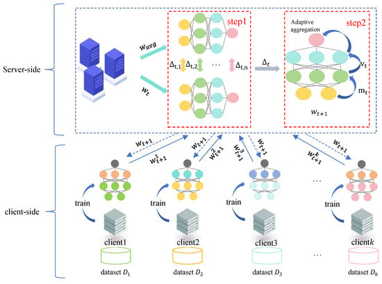
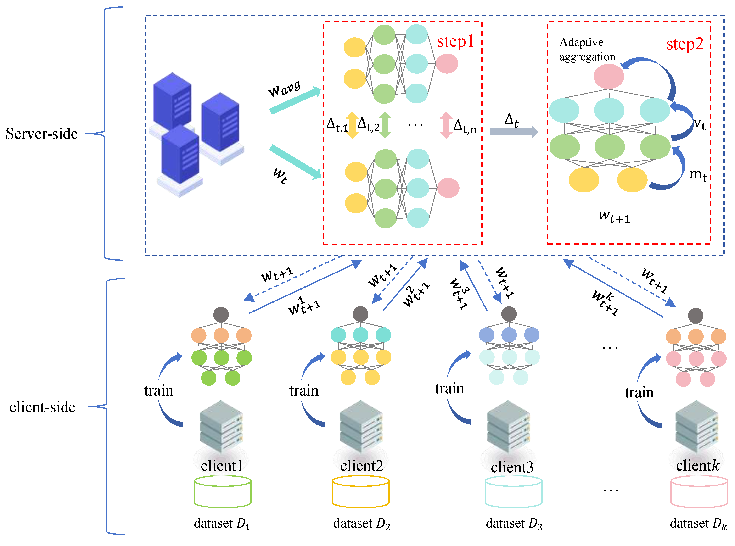
The SAPAA-MMF algorithm is designed to ensure that the global model aggregated by the server demonstrates robust performance and generalization capabilities. This paper leverages the complementary strengths of algorithms by integrating the improved joint mean algorithm with the adaptive aggregation algorithm. By combining the broad applicability and high performance of the joint mean algorithm with the adaptability and stability of the adaptive aggregation algorithm, the SAPAA-MMF algorithm further improves the performance and generalization capabilities of the global model. The overall architecture of SAPAA-MMF is depicted in Figure 1.

Figure 1. Architecture diagram of server-side adaptive parameter aggregation algorithm based on multi-method fusion.

The SAPAA-MMF algorithm operates within the federated learning framework developed in this study. As illustrated in Figure 1, each client utilizes its local dataset to perform distributed synchronous training, adhering to the standard federated learning process. After each training round, the aggregated global model is disseminated to the clients as updated model parameters, and iterative training continues until the termination condition is satisfied. During server-side aggregation, the hierarchical difference between the global model aggregated by the improved joint mean algorithm and the global model from the previous round is calculated. This difference is utilized as the pseudo-gradient for the adaptive aggregation algorithm, enabling it to generate a new global model with improved performance.

3.2. Objective Function

The local client device in federated learning is responsible solely for storing and processing data. Under this condition, it uploads the client model parameters to the server, which aggregates them to generate a single global model parameter w. In this distributed setting, the global optimization problem involves finding the set of parameters w that minimizes the average loss across all client devices participating in the training process. Thus, the global optimal objective function $F\left(w\right)$ on the server side can be expressed as

$$\underset{w}{min}F\left(w\right)={\displaystyle \frac{1}{K}}\sum _{k=1}^K{F}_k\left(w\right).$$

(1)

Here, K represents the total number of client devices participating in the joint training and $F_k\left(w\right)$ denotes the local objective function of the k-th client, which is expressed as

$$F_k\left(w\right)={\displaystyle \frac{1}{n_k}}\sum _{i\in d_k}{f}_i\left(w\right).$$

(2)

Here, $d_k$ represents the local dataset of the k-th client device, $n_k$ indicates the size of the k-th client’s data, and $f_i\left(w\right)$ refers to the loss value of the local client defect detection model SSD on sample i. The corresponding loss function $f\left(w\right)$ is expressed as

$$f\left(w\right)={\displaystyle \frac{1}{N}}(L_{conf}(w,x,c)+\lambda L_{loc}(w,x,l,g)),$$

(3)

where x is the matching indicator variable, c is the confidence score of each category predicted by the network, l is the offset of each default box predicted by the network relative to its original shape, and g represents the parameters of the real box, including the center coordinates $(cx,cy)$, width $\left(w\right)$, and height $\left(h\right)$. N is the number of default boxes corresponding to the matched real box, $L_{conf}$ is the classification loss, $L_{loc}$ is the positioning loss, and $\lambda$ is a hyperparameter that balances the weights between classification and positioning losses. $L_{conf}$ and $L_{loc}$ are calculated using Equation (4) and Equation (6), respectively. In Equation (3),

$$L_{conf}(w,x,c)=-\sum _{i\in Pos}^N{x}_{ij}^{p}log\left({\widehat{c}}_i^p\right)-\sum _{i\in Neg}log\left({\widehat{c}}_i^0\right),$$

(4)

where $x_{ij}^p=\{1,0\}$ indicates whether the i-th default box matches the real bounding box of category p. In Equation (4),

$${\widehat{c}}_i^p={\displaystyle \frac{exp\left(c_i^p\right)}{{\sum }_{p}exp\left(c_i^p\right)}}$$

(5)

indicates the probability that the i-th default box belongs to category p.

$$L_{loc}(w,x,l,g)=\sum _{i\in Pos}^N\sum _{m\in \{cx,cy,w,h\}}{x}_{ij}^f{smooth}_{\mathrm{L}1}\left(l_i^m-{\widehat{g}}_j^m\right),$$

(6)

where $x_{ij}^f=\{1,0\}$ indicates whether the i-th default box matches the j-th real bounding box. In Equation (6), ${smooth}_{\mathrm{L}1}(·)$ is the smooth L1 loss function used to calculate the difference in positional parameters between the bounding box predicted by the network and the real bounding box.

3.3. Algorithm Principle

The SAPAA-MMF algorithm integrates two algorithms to fully leverage the complementary strengths of different approaches, thereby enhancing the performance of the global model. This process is divided into two stages of aggregation. In the first stage, an improved joint mean algorithm is used for aggregation, followed by the calculation of hierarchical differences between the aggregated global model and the previous round’s global model. The objective is to leverage the adaptability and strong performance of the improved joint mean algorithm, fully accounting for the differences in client data and local training states, to obtain a high-performance one-stage global model. In the second stage, the hierarchical model differences from the first stage serve as pseudo-gradients for adaptive aggregation. The aim is to exploit the strong convergence and stability of adaptive aggregation algorithms to further enhance the stability and performance of the global model. Due to the use of joint mean and adaptive aggregation algorithms in multi-method fusion, this section primarily provides a detailed introduction and analysis of the joint mean algorithm, adaptive aggregation algorithm, and server-side adaptive parameter aggregation algorithm used in multi-method fusion.

3.3.1. Joint Mean Algorithm

McMahan et al. [6] proposed the joint mean algorithm FedAvg, applicable to horizontal federated learning. This algorithm accounts for the influence of data samples on aggregation performance, adapts to various environments, and fully utilizes the computing resources of diverse devices. By aggregating multiple local models, this algorithm enhances the model’s generalization ability and improves its robustness.

In the FedAvg algorithm, the server aggregates the model parameters uploaded by the clients, while the clients train the model on their local datasets. The detailed training process is as follows: First, the server initiates the global model’s initialization process and distributes the initialized model to various clients. Then, the server and clients jointly enter the iterative training stage. In the $t+1$ round of federated learning, the server selects K clients from all available clients for local model training and sends the aggregated global model $w_t$ from the t-th round to the selected clients. After receiving the global model, the clients train on their local datasets according to Equation (7). Finally, after local training, the local model parameters $w_{t+1}^k$ are generated as follows:

$$w_{t+1}^k=w_t^k-\eta g_k.$$

(7)

Here, $\eta$ represents the learning rate, and $g_k$ denotes the model gradient. After all client models complete training, the model parameters are uploaded to the server, which aggregates the parameters from each client model according to

$$w_{t+1}=\sum _{k=1}^K{\displaystyle \frac{n_k}{n}}·w_{t+1}^k.$$

(8)

Here, n represents the total number of client samples and $n_k$ denotes the number of samples for the k-th client. After server-side aggregation, a global model is generated and distributed to each client for subsequent rounds of training until the model converges or meets the termination condition.

3.3.2. Adaptive Aggregation Algorithm

The FedAdam algorithm, proposed by Reddi et al. [11], is a federated learning algorithm. It is an improved federated learning algorithm that utilizes the Adam optimizer [34] within the federated learning framework. It primarily addresses the issues of slow convergence, low accuracy, and poor stability encountered by traditional federated learning algorithms during model training.

The FedAdam algorithm is adapted from the Adam algorithm framework to accommodate the unique characteristics of federated learning. This algorithm retains the concept of adaptive learning rates from the Adam algorithm, dynamically adjusting the learning rate through first-order and second-order moment estimations to accelerate model convergence and improve stability. The formula for calculating the first-order moment in the FedAdam algorithm is:

$$m_t={\beta }_1{m}_{t-1}+(1-{\beta }_1){\Delta }_t$$

(9)

Here, t denotes the training round and ${\beta }_1$ represents the decay rate of first-order moment estimation. First-order moment estimation simulates the effect of momentum, helping to stabilize model parameter updates. Here, ${\Delta }_t$ represents the model pseudo-gradient. In the FedAdam algorithm, the average model difference for each client is computed as:

$${\Delta }_t^k=w_t^k-w_t.$$

(10)

Here, ${\Delta }_t^k$ represents the difference between the k-th client and the global model $w_t$ in round t. Based on the above equation, the average model difference ${\Delta }_t$ can be obtained as:

$${\Delta }_t={\displaystyle \frac{1}{\left|K\right|}}\sum _{i=1}^K{\Delta }_t^k.$$

(11)

The calculation formula for second-order moment estimation in the FedAdam algorithm is:

$$v_t={\beta }_2{v}_{t-1}+(1-{\beta }_2){\left({\Delta }_t\right)}^2.$$

(12)

Here, ${\beta }_2$ represents the decay rate of second-order moment estimation. By incorporating second-order moment estimation, the algorithm can more flexibly respond to gradient changes in the parameter space. In some cases, gradients can undergo significant changes, and second-order moment estimation captures this trend, facilitating learning rate adjustments and enhancing the algorithm’s robustness.

Finally, the formula for updating the model parameters is

$$w_{t+1}=w_t+{\displaystyle \frac{\sigma m_t}{\sqrt{v_t}+\tau }}.$$

(13)

Here, $\sigma$ represents the learning rate, controlling the magnitude of parameter updates, while $\tau$ is a small constant added for numerical stability to prevent division by zero.

3.3.3. A Server-Side Adaptive Parameter Aggregation Algorithm for Multi-Method Fusion

The first two sections provide a comprehensive introduction to the core concepts of the FedAvg and FedAdam algorithms. The FedAvg algorithm primarily addresses data distribution differences, offering strong effectiveness and adaptability, while the FedAdam algorithm focuses on improving model convergence speed and stability. Therefore, this paper posits that integrating these two algorithms can harness their complementary strengths, further enhancing the effectiveness of federated learning.

This paper proposes a server-side adaptive parameter aggregation algorithm, SAPAA-MMF, based on multi-method fusion. In the adaptive aggregation algorithm FedAdam, the pseudo-gradient ${\Delta }_t$ is calculated by averaging model differences, as shown in Equations (10) and (11). This paper posits that using average model differences as pseudo-gradients for adaptive aggregation overlooks the impact of client data samples on the global model. Since the number of data samples is a key factor in determining the contribution of each client, overlooking client data samples can result in weight allocation bias. For instance, clients with a large number of data samples may be undervalued, while clients with fewer data samples may be overvalued, leading to weight bias that can affect the accuracy of model training. Furthermore, overlooking client data samples can also diminish the model’s generalization ability. The diversity of data samples is crucial to the model’s generalization ability, and neglecting this factor may lead to poor model performance on new data. Therefore, during the model aggregation process, the influence of the number of client samples on the aggregation results must be carefully considered.

To address the above issues and integrate the advantages of different algorithms, this chapter adopts FedAdam as the base algorithm, incorporates the weighted client data samples from the FedAvg algorithm, and proposes a new model hierarchical difference as the pseudo-gradient ${\Delta }_t$ in the FedAdam algorithm:

$${\Delta }_t=[w_{avg,1}-w_{t,1},w_{avg,2}-w_{t,2},\dots ,w_{avg,i}-w_{t,i}].$$

(14)

Here, i represents the number of model layers, $w_{avg}$ denotes the global model aggregated using the joint mean algorithm in the first stage, and $w_t$ is the global model from the previous round. The detailed calculation of ${\Delta }_t$ is presented in Algorithm 1.

Algorithm 1: Calculation of hierarchical differences in models

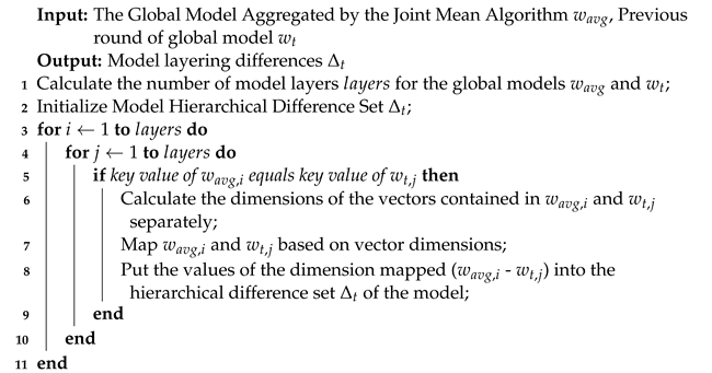Using hierarchical model differences that account for data samples as pseudo-gradients can effectively resolve the weight bias and generalization decline caused by average model differences. However, there are still challenges in calculating $w_{avg}$. In the calculation of $w_{avg}$, only the number of client samples is considered, meaning that the more samples a client has, the greater the client’s influence on the global model aggregation. If a client’s model parameters are of poor quality but the client has a large number of samples, this will negatively impact the performance of the global model.

In real-world federated learning, various factors influence client samples, including not only sample size but also differences in data distribution and quality. Therefore, the aggregation method for $w_{avg}$ can be further improved to fully account for the impact of factors such as client local data distribution and quality on the aggregation results. Since no direct indicator exists to measure data distribution and quality, the loss during client training is used as an indirect indicator to assess the local data distribution and quality factors of the client, further optimizing the calculation of

$$w_{avg}=\sum _{k=1}^K\left[\left(1-\theta \right)·{\displaystyle \frac{n_k}{n}}+\theta ·L_k\right]·w_{t+1}^k.$$

(15)

Here, $L_k$ represents the proportion of losses incurred by the k-th client relative to all clients. This improvement considers both the impact of local data samples and the loss incurred during training on the aggregation results. The parameter $\theta$ adjusts the ratio between sample size and loss. When $\theta$ equals 0, the calculation of $w_{avg}$ is equivalent to the original FedAvg algorithm. $L_k$ is calculated using Equation (16). In Equation (15),

$$L_k={\displaystyle \frac{e^{-l_k}}{{\sum }_{i=1}^K{e}^{-l_i}}},$$

(16)

where $l_i$ represents the model loss for the k-th client trained on the local dataset. This formula converts a set of losses into a probability distribution with values ranging between 0 and 1. For the exponential term $e^{-l_k}$, taking the negative value of the input $l_k$ ensures that smaller $l_k$ values approach 1 after the exponential operation, while larger $l_k$ values approach 0. Accordingly, for larger losses, if the model’s learning performance is poor, the proportion of losses should be small, whereas for smaller losses, if the model’s learning performance is good, the proportion of losses should be large.

Weight decay is a technique used to regularize neural networks, with its effects primarily manifesting in regularization, preventing overfitting, enhancing robustness, simplifying model structure, and improving convergence stability. By introducing weight decay, the model can learn simpler and smoother representations, thereby enhancing its generalization ability and robustness. Weight decay is introduced in the adaptive aggregation algorithm to prevent the global model parameters from becoming too large after server-side aggregation, thereby reducing the risk of overfitting and improving the stability and generalization performance of the global model. The weight decay penalty is introduced in the adaptive aggregation algorithm updates to control the complexity of the model. The optimized model update is given by:

$$w_{t+1}=w_t+\sigma \left({\displaystyle \frac{m_t}{\sqrt{v_t}+ϵ}}-\lambda w_t\right).$$

(17)

Here, $\lambda$ represents the weight decay term, which is a non-negative real number typically set to 0.0001 during training.

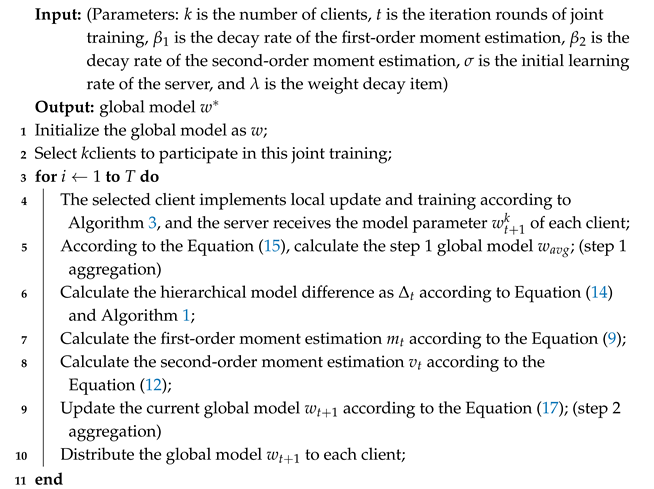
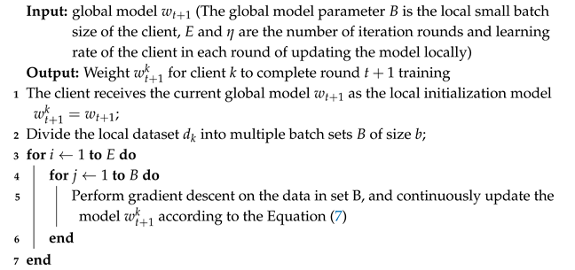
Based on the aforementioned algorithm steps and fundamental principles, a server-side adaptive parameter aggregation algorithm for multi-method fusion has been implemented. The detailed steps of the algorithm are presented in Algorithm 2. Algorithm 3 provides the client-side update procedure, which is used to receive the global model and perform updates and local training.

Algorithm 2: A server-side adaptive parameter aggregation algorithm for multi-method fusion (SAPAA-MMF)

Algorithm 3: Client update algorithm

3.3.4. Algorithm Flow

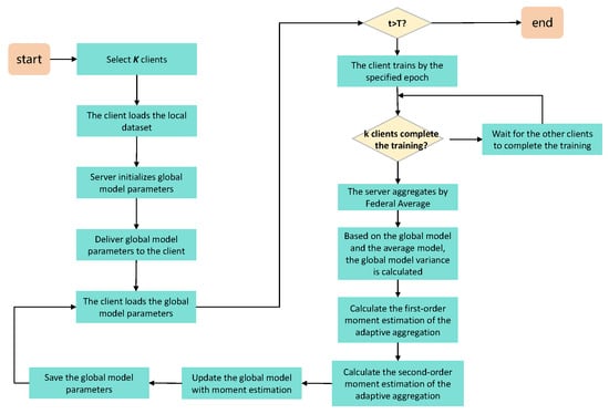
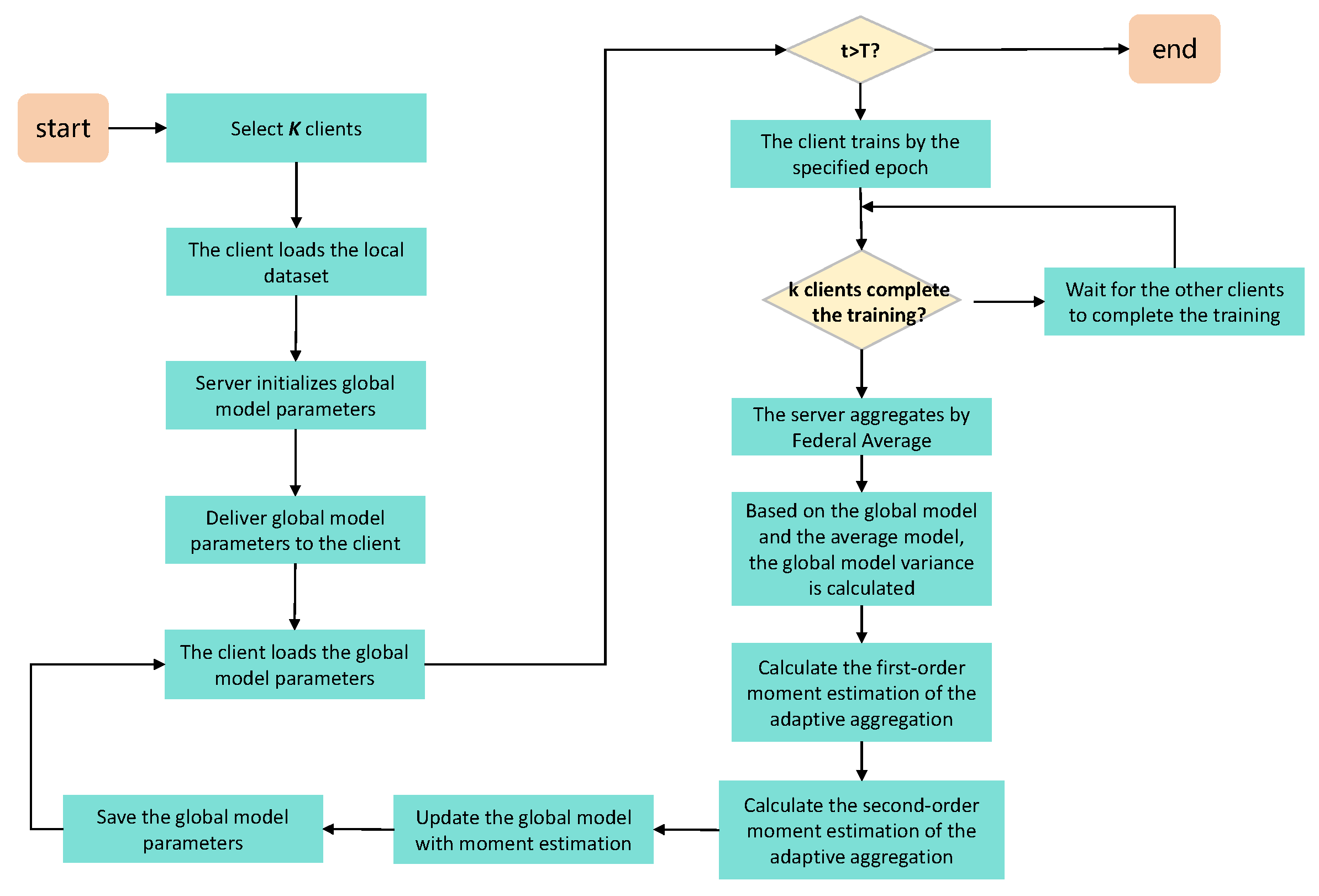
Combining the SAPAA-MMF algorithm with the basic process of federated learning, the specific algorithm process is illustrated in Figure 2. Initially, the server selects k clients for joint training. Each client loads its local dataset and waits for the initialization of the model. Once the server initializes the model, it distributes the global model to each client. After receiving the initialized global model, clients load it and use it as their initial model parameters for training. After the initialization phase, the training proceeds according to the specified number of rounds. If training reaches the specified number of rounds, the joint training task ends. Otherwise, each client uses its local dataset for training and waits for all k clients to complete their training, after which the server aggregates the k models. In the SAPAA-MMF algorithm, the improved joint mean algorithm is first used to aggregate and obtain a one-stage global model. The hierarchical model difference is subsequently calculated based on the previous round’s global model. This hierarchical model difference is used as a pseudo-gradient to calculate the first-order moment estimation and the second-order moment estimation. A two-stage global model is generated through adaptive aggregation, and the global model parameters for the current round are stored. This process constitutes one round of SAPAA-MMF training. Iterative training continues until the specified number of rounds is reached or the model converges, at which point the training concludes.

Figure 2. SAPAA-MMF algorithm flow chart.

3.3.5. Algorithm Complexity Analysis

SAPAA-MMF is a federated learning algorithm that operates within the federated learning framework, with its primary task being model aggregation. Therefore, this section will not consider the complexity of the federated learning framework but will focus solely on analyzing the time and space complexity of the SAPAA-MMF algorithm. In terms of time complexity, the primary factor affecting the complexity of the SAPAA-MMF algorithm is the number of model layers, denoted as m. The algorithm first iterates through the model layers for one-stage aggregation, resulting in a time complexity of $O\left(m\right)$. Next, the hierarchical model difference is calculated. Since the model layers need to be matched, the time complexity of this step is $O\left(m^2\right)$. Finally, the adaptive algorithm aggregates the two-stage model, with a time complexity of $O\left(m\right)$. Therefore, the overall time complexity of the SAPAA-MMF algorithm is $O(m^2+2m)$, which simplifies to $O\left(m^2\right)$. In terms of space complexity, the primary factor influencing the complexity of the SAPAA-MMF algorithm is the number of model layers, denoted as m. The algorithm requires loading all the models into the memory during execution. Therefore, the space complexity of the algorithm is $O\left(m\right)$.

4. Experiments

4.1. Experiments Setup

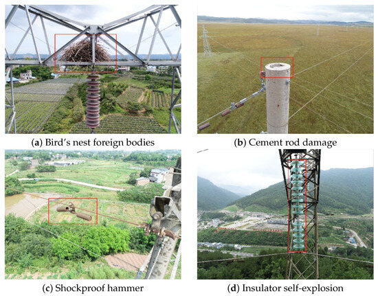
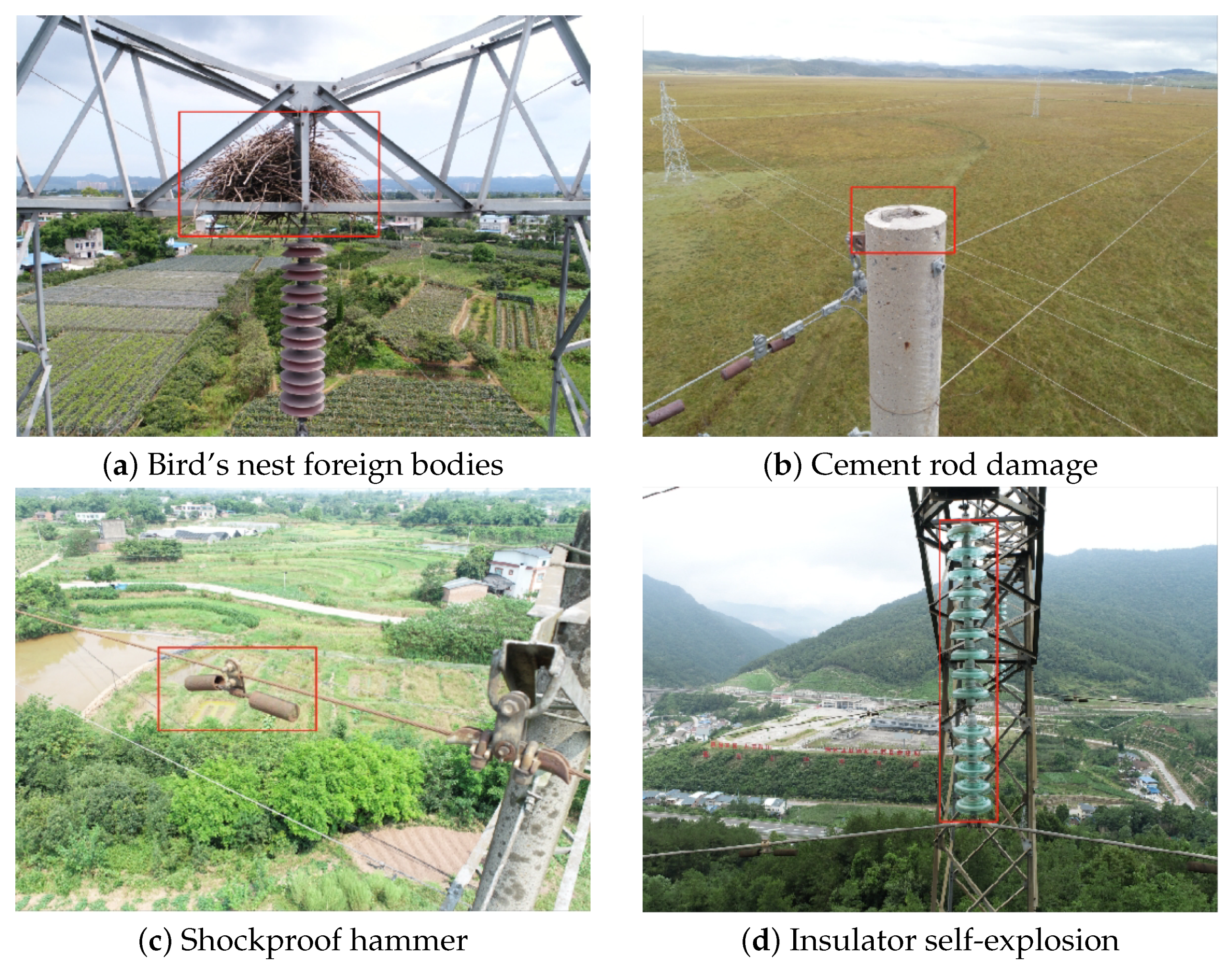
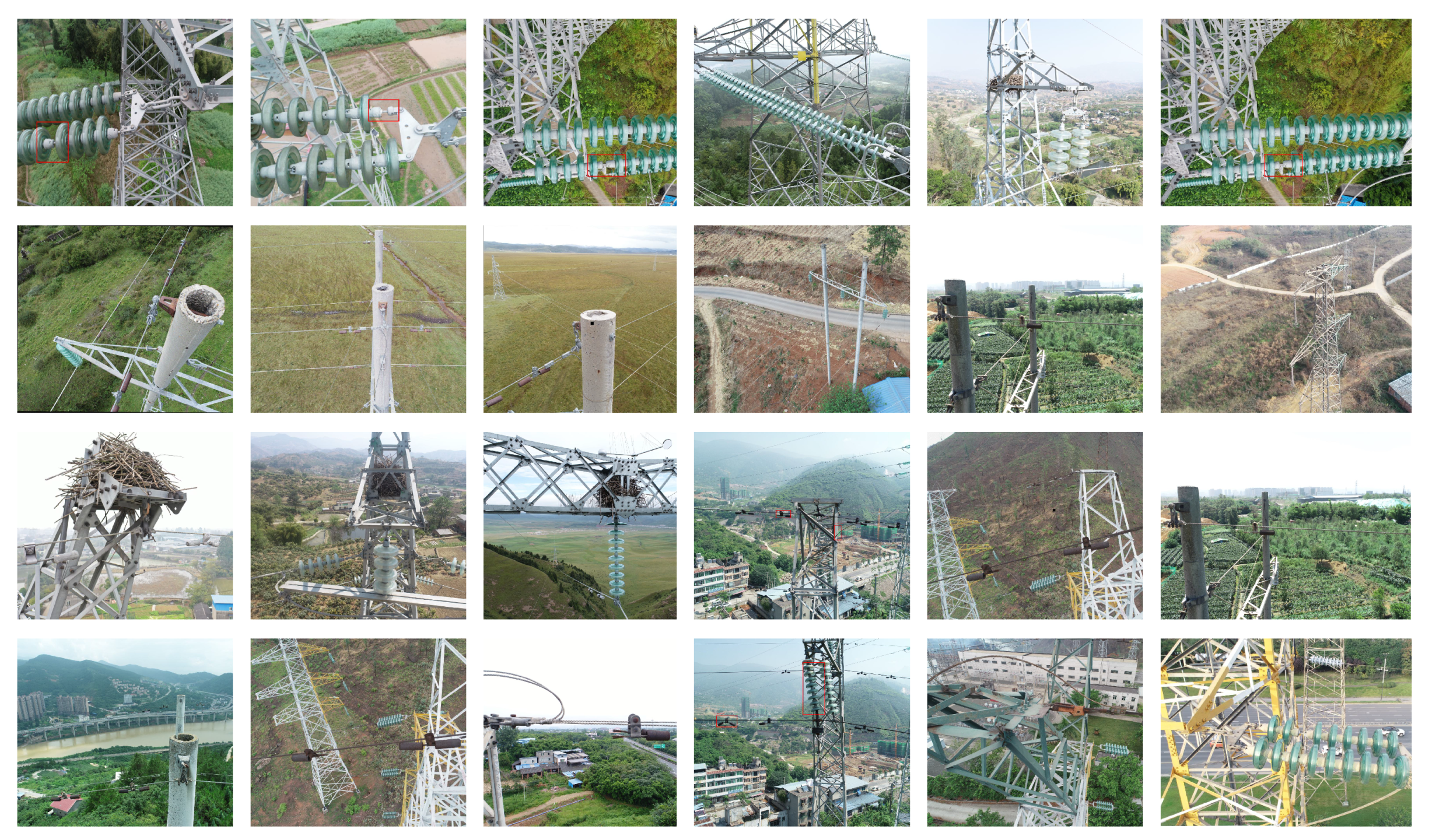
Datasets. This paper utilizes transmission line defect data as the experimental dataset, provided by the State Grid Sichuan Electric Power Company Electric Power Research Institute. After thorough screening and collation, the defect data has been meticulously marked and reviewed by professionals, ensuring its high quality and credibility, thereby accurately reflecting various transmission line defects in actual operation. The entire dataset is categorized based on defect characteristics, comprising four main types: bird’s nest foreign bodies, cement rod damage, shockproof hammer slip, and insulator self-explosion. To enable efficient detection of multiple defects using a single model, the four types of defect data are combined into a mixed dataset containing various defect types. Table 1 illustrates the details of all the datasets. Figure 3 and Figure 4 present sample images of the four defect types and the mixed dataset, respectively.

Table 1. Defect dataset information.

Dataset	client_1	client_2	client_3	client_4	Total
Bird’s nest foreign bodies	115	115	115	36	381
Cement rod damage	90	100	110	23	323
Shockproof hammer slip	85	105	115	29	334
Insulator self-explosion	114	93	106	26	339
Mixed dataset	175	175	175	54	579

Figure 3. Examples of datasets. The image dataset was obtained from the State Grid Sichuan Electric Power Research Institute, Power Internet of Things Key Laboratory of Sichuan Province.

Figure 4. Mixed data example. The image dataset was obtained from the State Grid Sichuan Electric Power Research Institute, Power Internet of Things Key Laboratory of Sichuan Province.

As shown in Table 1, federated learning involves multiple clients and requires distributed training. Therefore, this paper divides the five datasets into four parts, each of which is used as local data for individual clients. Client_4 is designated for global evaluation and does not participate in model training.

Software and hardware environment. The experimental environment is divided into a hardware environment and a software environment. The host using the Ubuntu operating system on the hardware uses system version number 18.04 and has a memory size of 86 G, a CPU of AMD EPYC 7402, a graphics card of NVIDIA A40 (19.5 TFLOPs), and a video memory size of 48G. The programming language of the software is python, version 3.8. The depth learning framework used is python, version 1.9. The programming IDE is Pycharm 2023.2.

Experimental framework. On the experimental framework, Flower is used as the basic framework for federated learning and the SSD network is used as the transmission line defect detection model to build a multi-client transmission line defect detection federated learning synchronous training framework.

Comparison Algorithms. The SAPAA-MMF algorithm proposed in this paper is used for federated learning, and compared with FedAvg [11], FedAvgM [35], FedYogi [11], FedAdam [11], FedAdagrad [11], FedMedia [22], TrimmedAvg [22], and Krum [21] algorithms.

Parameter settings. The initial learning rate of the SSD network is set to 0.002, the Batchsize is set to 2, 20 epochs are trained in each round, a total of 20 rounds, and 1200 epochs are trained for three clients. The initialization parameter of SAPAA-MMF algorithm $\theta$ is set to 0.003, ${\beta }_1$ is set to 0.9, ${\beta }_2$ is set to 0.99, and $\sigma$ is set to 0.01.

Evaluation metrics. The experimental results are evaluated and compared separately for the server and client. Server evaluation measures the performance of the global model, while client evaluation assesses the performance of the client model. The client evaluation result is obtained by averaging all client evaluations. For evaluation metrics, five indicators—$AP$, $A{P}_{50}$, $A{P}_{75}$, $A{R}_{100}$, and $A{R}_{300}$—which effectively represent the model’s performance, are selected. These five indicators are standard metrics from the COCO dataset [36]. Detailed definitions of these evaluation metrics are provided in the next subsection.

4.2. Evaluation Metrics Definition

In this paper, a target detection model is used to identify transmission line defects and a federated learning model for defect detection is trained using the federated learning algorithm. Therefore, the evaluation metrics used in this paper are commonly employed in target detection and the effectiveness of the proposed federated learning algorithm is assessed using these metrics. The commonly used evaluation metrics in target detection include AP and AR values. These evaluation metrics are described below.

Intersection over Union ($IoU$) is a metric commonly used to evaluate the degree of overlap between bounding boxes in target detection. $IoU$ calculates the ratio of the overlapping area between two bounding boxes to their union. It is typically used to evaluate the match between the predicted bounding box and the actual target box. The formula is as follows:

$$IoU={\displaystyle \frac{area(B_p\cap B_{gt})}{area(B_p\cup B_{gt})}}.$$

(18)

Here, $B_p$ represents the predicted box, $B_{gt}$ is the actual target box, and the $IoU$ value ranges from 0 to 1.

Generally, in target detection, when the Intersection over Union ($IoU$) between the predicted box and the ground truth box exceeds the threshold of 0.5, the predicted box is considered a positive sample. Conversely, if the $IoU$ is lower than 0.5, the predicted box is considered a negative sample. Under this standard, the instances that the model correctly identifies as positive samples are defined as true positives ($TP$), while the instances correctly identified as negative samples are referred to as true negatives ($TN$). Conversely, when an actual positive sample is mistakenly classified as negative by the model, it is recorded as a false negative ($FN$). Similarly, when an actual negative sample is mistakenly classified as positive, it is recorded as a false positive ($FP$). Based on the above, Precision and Recall can be calculated using the following formulas:

$$Precision={\displaystyle \frac{TP}{TP+FP}},$$

(19)

$$Recall={\displaystyle \frac{TP}{TP+FN}}.$$

(20)

The Precision–Recall ($PR$) curve illustrates the trade-off between these two metrics as the threshold changes, making it a common method for evaluating the effectiveness of classification models. Average precision ($AP$) is the area under the $PR$ curve, obtained by integrating the area enclosed by the $PR$ curve and the coordinate axes, and serves as a measure of the model’s overall performance. The larger the area value, the better the overall performance of the detection model. Its calculation formula is as follows:

$$AP={\int }_0^{1}P\left(r\right)dr.$$

(21)

In target detection tasks, $AP$ is an important evaluation metric, typically calculated based on different $IoU$ thresholds. These thresholds include $A{P}_{50}$ and $A{P}_{75}$, which represent the average precision when the $IoU$ threshold is 0.5 and 0.75, respectively. Additionally, an $IoU$ step of 0.05 can be used to calculate $AP$ values from $A{P}_{50}$ to $A{P}_{95}$, with the average taken as $A{P}_{50:95}$. The model’s performance can be evaluated using multiple metrics at different thresholds.

Average recall ($AR$) is the average of all $Recall$ values within the $IoU$ range of [0.5, 1], used to evaluate the recall performance of the detection model. The calculation formula is as follows:

$$AR=2{\int }_{0.5}^{1}recall\left(o\right)do$$

(22)

In target detection tasks, the maximum number of targets to be detected is often limited. Therefore, metrics such as $A{R}_{100}$ and $A{R}_{300}$ are typically used to represent the average recall when the number of detections is limited to 100, 300, and so on, to more comprehensively evaluate the performance of the detection model.

4.3. Comparison of Server Evaluation

This section will compare the performance of SAPAA-MMF algorithm and each comparison algorithm in the server evaluation using five datasets.

The server evaluation results based on the Bird’s Nest Foreign Bodies dataset are presented in Table 2. From this dataset, it is evident that the SAPAA-MMF algorithm ranks first in four of the server evaluation metrics. The $AP$, $A{P}_{50}$, $A{R}_{100}$, and $A{R}_{300}$ metrics outperform those of the other comparison algorithms. Although $A{P}_{75}$ is lower than the maximum value among the comparison algorithms, the overall $Average$ value remains higher than that of the other comparison algorithms.

Table 2. The server evaluation results of each algorithm, based on the Bird’s Nest Foreign Bodies dataset.

Algorithm	Indicator
	$\mathit{AP}$	${\mathit{AP}}_{\mathbf{50}}$	${\mathit{AP}}_{\mathbf{75}}$	${\mathit{AR}}_{\mathbf{100}}$	${\mathit{AR}}_{\mathbf{300}}$	$\mathit{Average}$
FedAvg	0.166	0.497	0.070	0.260	0.265	0.252
FedAvgM	0.185	0.455	0.114	0.265	0.265	0.257
FedYogi	0.182	0.483	0.079	0.240	0.240	0.245
FedAdam	0.174	0.506	0.063	0.247	0.247	0.247
FedAdagrad	0.196	0.503	0.074	0.255	0.255	0.257
FedMedia	0.171	0.496	0.094	0.243	0.243	0.249
TrimmedAvg	0.197	0.469	0.156	0.265	0.265	0.270
Krum	0.138	0.443	0.047	0.217	0.232	0.215
SAPAA-MMF	0.202	0.509	0.123	0.267	0.267	0.274

The server evaluation results based on the Cement Rod Damage dataset are presented in Table 3. From this dataset, it is evident that the SAPAA-MMF algorithm ranks first in four of the server evaluation metrics. The $AP$, $A{P}_{50}$, $A{R}_{100}$, and $A{R}_{300}$ metrics outperform those of the other comparison algorithms. Although $A{P}_{75}$ is lower than the maximum value among the comparison algorithms, the overall $Average$ value remains higher than that of the other comparison algorithms.

Table 3. The server evaluation results of each algorithm, based on the Cement Rod Damage dataset.

Algorithm	Indicator
	$\mathit{AP}$	${\mathit{AP}}_{\mathbf{50}}$	${\mathit{AP}}_{\mathbf{75}}$	${\mathit{AR}}_{\mathbf{100}}$	${\mathit{AR}}_{\mathbf{300}}$	$\mathit{Average}$
FedAvg	0.601	0.783	0.752	0.633	0.650	0.684
FedAvgM	0.543	0.776	0.703	0.588	0.588	0.640
FedYogi	0.597	0.793	0.754	0.642	0.642	0.686
FedAdam	0.602	0.776	0.752	0.604	0.604	0.668
FedAdagrad	0.534	0.771	0.567	0.567	0.567	0.601
FedMedia	0.577	0.763	0.752	0.613	0.613	0.664
TrimmedAvg	0.540	0.786	0.621	0.596	0.596	0.628
Krum	0.522	0.727	0.655	0.567	0.567	0.608
SAPAA-MMF	0.614	0.795	0.752	0.654	0.654	0.694

The server evaluation results based on the Shockproof Hammer Slip dataset are presented in Table 4. The SAPAA-MMF algorithm ranks first in all five server evaluation metrics: $AP$, $A{P}_{50}$, $A{P}_{75}$, $A{R}_{100}$, and $A{R}_{300}$, outperforming the other comparison algorithms.

Table 4. The server evaluation results of each algorithm, based on the Shockproof Hammer Slip dataset.

Algorithm	Indicator
	$\mathit{AP}$	${\mathit{AP}}_{\mathbf{50}}$	${\mathit{AP}}_{\mathbf{75}}$	${\mathit{AR}}_{\mathbf{100}}$	${\mathit{AR}}_{\mathbf{300}}$	$\mathit{Average}$
FedAvg	0.443	0.692	0.499	0.521	0.521	0.535
FedAvgM	0.440	0.691	0.478	0.514	0.514	0.527
FedYogi	0.445	0.700	0.498	0.545	0.545	0.547
FedAdam	0.438	0.703	0.521	0.521	0.534	0.543
FedAdagrad	0.264	0.629	0.116	0.393	0.393	0.359
FedMedia	0.398	0.714	0.414	0.497	0.497	0.504
TrimmedAvg	0.439	0.699	0.554	0.507	0.507	0.541
Krum	0.310	0.673	0.288	0.393	0.400	0.412
SAPAA-MMF	0.446	0.716	0.586	0.552	0.552	0.570

The server evaluation results based on the Insulator Self-Explosion dataset are presented in Table 5. From this dataset, it is evident that the SAPAA-MMF algorithm ranks first in four of the server evaluation metrics. The $AP$, $A{P}_{50}$, $A{R}_{100}$, and $A{R}_{300}$ metrics outperform those of the other comparison algorithms. Although $A{P}_{75}$ is lower than the maximum value among the comparison algorithms, the overall $Average$ value remains higher than that of the other comparison algorithms.

Table 5. The server evaluation results of each algorithm, based on the Insulator Self-Explosion dataset.

Algorithm	Indicator
	$\mathit{AP}$	${\mathit{AP}}_{\mathbf{50}}$	${\mathit{AP}}_{\mathbf{75}}$	${\mathit{AR}}_{\mathbf{100}}$	${\mathit{AR}}_{\mathbf{300}}$	$\mathit{Average}$
FedAvg	0.261	0.463	0.273	0.355	0.370	0.344
FedAvgM	0.293	0.523	0.349	0.385	0.391	0.388
FedYogi	0.346	0.528	0.381	0.391	0.391	0.407
FedAdam	0.330	0.517	0.407	0.370	0.376	0.400
FedAdagrad	0.256	0.531	0.260	0.300	0.300	0.329
FedMedia	0.264	0.445	0.333	0.370	0.370	0.356
TrimmedAvg	0.314	0.526	0.371	0.397	0.397	0.401
Krum	0.274	0.526	0.304	0.373	0.376	0.371
SAPAA-MMF	0.349	0.533	0.394	0.398	0.398	0.414

The server evaluation results based on the mixed dataset are presented in Table 6. From this dataset, it is evident that the SAPAA-MMF algorithm ranks first in three of the server evaluation metrics. The $AP$, $A{P}_{50}$, and $A{P}_{75}$ metrics outperform those of the other comparison algorithms. Although $A{R}_{100}$ and $A{R}_{300}$ are lower than the maximum values among the comparison algorithms, the overall $Average$ value remains higher than that of the other comparison algorithms.

Table 6. The server evaluation results of each algorithm, based on the mixed dataset.

Algorithm	Indicator
	$\mathit{AP}$	${\mathit{AP}}_{\mathbf{50}}$	${\mathit{AP}}_{\mathbf{75}}$	${\mathit{AR}}_{\mathbf{100}}$	${\mathit{AR}}_{\mathbf{300}}$	$\mathit{Average}$
FedAvg	0.320	0.598	0.344	0.394	0.394	0.410
FedAvgM	0.311	0.570	0.301	0.394	0.394	0.394
FedYogi	0.290	0.581	0.262	0.356	0.356	0.369
FedAdam	0.332	0.628	0.365	0.368	0.368	0.412
FedAdagrad	0.342	0.651	0.299	0.368	0.368	0.406
FedMedia	0.290	0.562	0.321	0.397	0.397	0.393
TrimmedAvg	0.284	0.580	0.301	0.392	0.397	0.391
Krum	0.263	0.564	0.252	0.363	0.365	0.361
SAPAA-MMF	0.346	0.653	0.370	0.396	0.396	0.432

From Table 2, Table 3, Table 4, Table 5 and Table 6, it is evident that the SAPAA-MMF algorithm consistently achieves the best results across the five datasets in the server evaluation, excelling in key metrics such as $AP$, $A{P}_{50}$, $A{P}_{75}$, $A{R}_{100}$, and $A{R}_{300}$. Notably, the $AP$ and $A{P}_{50}$ metrics consistently rank first across all datasets, and the overall average value of all SAPAA-MMF indicators remains higher than those of the comparison algorithms. This consistent performance highlights the superiority of the SAPAA-MMF algorithm, demonstrating its innovation and advancement over traditional methods. The SAPAA-MMF algorithm, as a multi-method fusion federated learning approach, leverages the strengths of different algorithms to achieve superior performance. In the one-stage aggregation process, it effectively balances the impact of data sample size and training loss, leading to strong initial results. The two-stage adaptive aggregation further enhances the stability of the training process, ensuring that the model not only performs well but also exhibits robust generalization capabilities. Consequently, the SAPAA-MMF algorithm produces a federated learning model that excels in defect detection, significantly improving both detection accuracy and generalization across diverse datasets.

4.4. Comparison of Client Evaluation

This section will compare the performance of the SAPAA-MMF algorithm with that of each comparison algorithm in the client evaluation using five datasets.

The client evaluation results based on the Bird’s Nest Foreign Bodies dataset are presented in Table 7. From this dataset, it is evident that the SAPAA-MMF algorithm ranks first in three of the client evaluation metrics. The $AP$, $A{P}_{50}$, and $A{P}_{75}$ metrics outperform those of the other comparison algorithms. Although $A{R}_{100}$ and $A{R}_{300}$ are lower than the maximum values among the comparison algorithms, the overall $Average$ value remains higher than that of the other comparison algorithms.

Table 7. The client evaluation results of each algorithm, based on the Bird’s Nest Foreign Bodies dataset.

Algorithm	Indicator
	$\mathit{AP}$	${\mathit{AP}}_{\mathbf{50}}$	${\mathit{AP}}_{\mathbf{75}}$	${\mathit{AR}}_{\mathbf{100}}$	${\mathit{AR}}_{\mathbf{300}}$	$\mathit{Average}$
FedAvg	0.214	0.571	0.121	0.287	0.289	0.296
FedAvgM	0.224	0.585	0.175	0.318	0.318	0.324
FedYogi	0.203	0.551	0.147	0.303	0.303	0.302
FedAdam	0.214	0.564	0.140	0.281	0.282	0.296
FedAdagrad	0.219	0.589	0.155	0.281	0.281	0.305
FedMedia	0.217	0.587	0.136	0.316	0.316	0.314
TrimmedAvg	0.224	0.562	0.160	0.316	0.319	0.316
Krum	0.203	0.518	0.135	0.295	0.305	0.291
SAPAA-MMF	0.244	0.597	0.178	0.317	0.317	0.331

The client evaluation results based on the Cement Rod Damage dataset are presented in Table 8. The SAPAA-MMF algorithm ranks first in all five client evaluation metrics, $AP$, $A{P}_{50}$, $A{P}_{75}$, $A{R}_{100}$, and $A{R}_{300}$, outperforming the other comparison algorithms.

Table 8. The client evaluation results of each algorithm, based on the Cement Rod Damage dataset.

Algorithm	Indicator
	$\mathit{AP}$	${\mathit{AP}}_{\mathbf{50}}$	${\mathit{AP}}_{\mathbf{75}}$	${\mathit{AR}}_{\mathbf{100}}$	${\mathit{AR}}_{\mathbf{300}}$	$\mathit{Average}$
FedAvg	0.611	0.837	0.720	0.659	0.659	0.697
FedAvgM	0.609	0.811	0.749	0.653	0.655	0.695
FedYogi	0.605	0.847	0.718	0.667	0.667	0.701
FedAdam	0.564	0.853	0.703	0.631	0.631	0.676
FedAdagrad	0.516	0.822	0.546	0.566	0.566	0.603
FedMedia	0.604	0.851	0.683	0.671	0.674	0.697
TrimmedAvg	0.597	0.853	0.692	0.650	0.650	0.688
Krum	0.569	0.780	0.708	0.618	0.619	0.659
SAPAA-MMF	0.621	0.867	0.758	0.677	0.678	0.720

The client evaluation results based on the Shockproof Hammer Slip dataset are presented in Table 9. From this dataset, it is evident that the SAPAA-MMF algorithm ranks first in four of the client evaluation metrics. The $AP$, $A{P}_{50}$, $A{R}_{100}$, and $A{R}_{300}$ metrics outperform those of the other comparison algorithms. The overall $Average$ value remains higher than that of the other comparison algorithms.

Table 9. The client evaluation results of each algorithm, based on the Shockproof Hammer Slip dataset.

Algorithm	Indicator
	$\mathit{AP}$	${\mathit{AP}}_{\mathbf{50}}$	${\mathit{AP}}_{\mathbf{75}}$	${\mathit{AR}}_{\mathbf{100}}$	${\mathit{AR}}_{\mathbf{300}}$	$\mathit{Average}$
FedAvg	0.473	0.751	0.500	0.544	0.544	0.562
FedAvgM	0.465	0.746	0.554	0.541	0.541	0.569
FedYogi	0.470	0.771	0.567	0.532	0.532	0.574
FedAdam	0.436	0.707	0.506	0.523	0.523	0.539
FedAdagrad	0.276	0.641	0.178	0.370	0.376	0.368
FedMedia	0.466	0.767	0.499	0.534	0.534	0.560
TrimmedAvg	0.441	0.732	0.471	0.505	0.505	0.531
Krum	0.403	0.730	0.425	0.504	0.504	0.513
SAPAA-MMF	0.473	0.772	0.559	0.553	0.553	0.582

The client evaluation results based on the Insulator Self-Explosion dataset are presented in Table 10. From this dataset, it is evident that the SAPAA-MMF algorithm ranks first in four of the client evaluation metrics. The $AP$, $A{P}_{75}$, $A{R}_{100}$, and $A{R}_{300}$ metrics outperform those of the other comparison algorithms. The overall $Average$ value remains higher than that of the other comparison algorithms.

Table 10. The client evaluation results of each algorithm, based on the Insulator Self-Explosion dataset.

Algorithm	Indicator
	$\mathit{AP}$	${\mathit{AP}}_{\mathbf{50}}$	${\mathit{AP}}_{\mathbf{75}}$	${\mathit{AR}}_{\mathbf{100}}$	${\mathit{AR}}_{\mathbf{300}}$	$\mathit{Average}$
FedAvg	0.263	0.485	0.262	0.357	0.361	0.346
FedAvgM	0.275	0.503	0.284	0.372	0.378	0.362
FedYogi	0.316	0.554	0.320	0.377	0.378	0.389
FedAdam	0.318	0.539	0.344	0.366	0.370	0.387
FedAdagrad	0.255	0.529	0.256	0.334	0.335	0.342
FedMedia	0.210	0.434	0.166	0.319	0.325	0.291
TrimmedAvg	0.275	0.522	0.300	0.353	0.360	0.362
Krum	0.233	0.461	0.236	0.340	0.348	0.324
SAPAA-MMF	0.328	0.539	0.348	0.381	0.389	0.397

The client evaluation results based on the mixed dataset are presented in Table 11. From this dataset, it is evident that the SAPAA-MMF algorithm ranks first in four of the client evaluation metrics. The $AP$, $A{P}_{50}$, $A{R}_{100}$, and $A{R}_{300}$ metrics outperform those of the other comparison algorithms. Although $A{P}_{75}$ is lower than the maximum value among the comparison algorithms, the overall $Average$ value remains higher than that of the other comparison algorithms.

Table 11. The client evaluation results of each algorithm, based on the mixed dataset.

Algorithm	Indicator
	$\mathit{AP}$	${\mathit{AP}}_{\mathbf{50}}$	${\mathit{AP}}_{\mathbf{75}}$	${\mathit{AR}}_{\mathbf{100}}$	${\mathit{AR}}_{\mathbf{300}}$	$\mathit{Average}$
FedAvg	0.263	0.534	0.208	0.379	0.381	0.353
FedAvgM	0.277	0.518	0.215	0.382	0.382	0.355
FedYogi	0.270	0.516	0.262	0.341	0.341	0.346
FedAdam	0.265	0.537	0.238	0.334	0.334	0.342
FedAdagrad	0.278	0.537	0.216	0.346	0.346	0.345
FedMedia	0.280	0.527	0.239	0.364	0.364	0.355
TrimmedAvg	0.264	0.514	0.230	0.369	0.372	0.350
Krum	0.227	0.498	0.181	0.333	0.333	0.314
SAPAA-MMF	0.285	0.540	0.240	0.383	0.384	0.366

From Table 7, Table 8, Table 9, Table 10 and Table 11, it is evident that the SAPAA-MMF algorithm consistently achieves the best results across the five client evaluation metrics: $AP$, $A{P}_{50}$, $A{P}_{75}$, $A{R}_{100}$, and $A{R}_{300}$ on the five datasets. The $AP$ metric consistently ranks first across all five datasets, and the average value of all metrics for the SAPAA-MMF algorithm remains higher than that of the other comparison algorithms. SAPAA-MMF combines the strengths of multiple algorithms and enhances the server evaluation, resulting in a better global model. This indicates that the global model performs better across the entire dataset, demonstrating strong generalization capabilities and consistent performance across different data distributions. As a result, client evaluation has also improved, further confirming that the global model exhibits strong generalization capabilities on client data. This underscores the effectiveness and innovation of the SAPAA-MMF algorithm, which consistently delivers strong performance and generalization.

4.5. Hyper-Parameter Experimental Verification

In the SAPAA-MMF algorithm, factors such as data distribution, data quality, and the number of samples also influence the effectiveness of parameter aggregation. Since there is no direct indicator to measure these factors, the client training loss is used as an indirect measure of local data distribution and quality. In the SAPAA-MMF algorithm, the hyperparameter $\theta$ is used to control the balance between sample size and loss during parameter aggregation. The optimal value of the hyperparameter $\theta$ is determined through experiments, validating the rationale for using client loss as a condition for parameter aggregation. Table 12 and Table 13 in the mixed dataset present the optimal values of the hyperparameter $\theta$ for server and client evaluations across different metrics, including $AP$, $A{P}_{50}$, $A{P}_{75}$, $A{R}_{100}$, and $A{R}_{300}$.

Table 12. Optimal indicators for server evaluation with different parameter values based on mixed datasets.

Parameter	Indicator
	$\mathit{AP}$	${\mathit{AP}}_{\mathbf{50}}$	${\mathit{AP}}_{\mathbf{75}}$	${\mathit{AR}}_{\mathbf{100}}$	${\mathit{AR}}_{\mathbf{300}}$	$\mathit{Average}$
$\theta =0$	0.335	0.624	0.339	0.390	0.390	0.416
$\theta =0.001$	0.304	0.649	0.275	0.400	0.400	0.406
$\theta =0.003$	0.346	0.653	0.370	0.396	0.396	0.432
$\theta =0.005$	0.329	0.550	0.352	0.397	0.397	0.405
$\theta =0.007$	0.320	0.629	0.252	0.411	0.411	0.405
$\theta =0.009$	0.316	0.626	0.303	0.403	0.403	0.410
$\theta =0.01$	0.319	0.570	0.314	0.399	0.399	0.400
$\theta =0.03$	0.244	0.515	0.196	0.373	0.378	0.341
$\theta =0.05$	0.198	0.433	0.131	0.343	0.346	0.290
$\theta =0.07$	0.131	0.339	0.112	0.273	0.273	0.226
$\theta =0.09$	0.107	0.269	0.088	0.255	0.257	0.195

Table 13. Optimal indicators for client evaluation with different parameter values based on mixed datasets.

Parameter	Indicator
	$\mathit{AP}$	${\mathit{AP}}_{\mathbf{50}}$	${\mathit{AP}}_{\mathbf{75}}$	${\mathit{AR}}_{\mathbf{100}}$	${\mathit{AR}}_{\mathbf{300}}$	$\mathit{Average}$
$\theta =0$	0.284	0.539	0.271	0.326	0.326	0.349
$\theta =0.001$	0.278	0.533	0.271	0.331	0.331	0.349
$\theta =0.003$	0.285	0.540	0.240	0.383	0.384	0.366
$\theta =0.005$	0.287	0.520	0.259	0.352	0.352	0.354
$\theta =0.007$	0.277	0.546	0.265	0.351	0.351	0.358
$\theta =0.009$	0.275	0.534	0.281	0.347	0.347	0.357
$\theta =0.01$	0.278	0.531	0.248	0.351	0.351	0.352
$\theta =0.03$	0.251	0.546	0.190	0.358	0.358	0.341
$\theta =0.05$	0.186	0.459	0.115	0.304	0.305	0.274
$\theta =0.07$	0.135	0.358	0.070	0.291	0.291	0.229
$\theta =0.09$	0.091	0.280	0.049	0.206	0.206	0.166

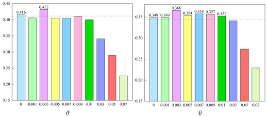
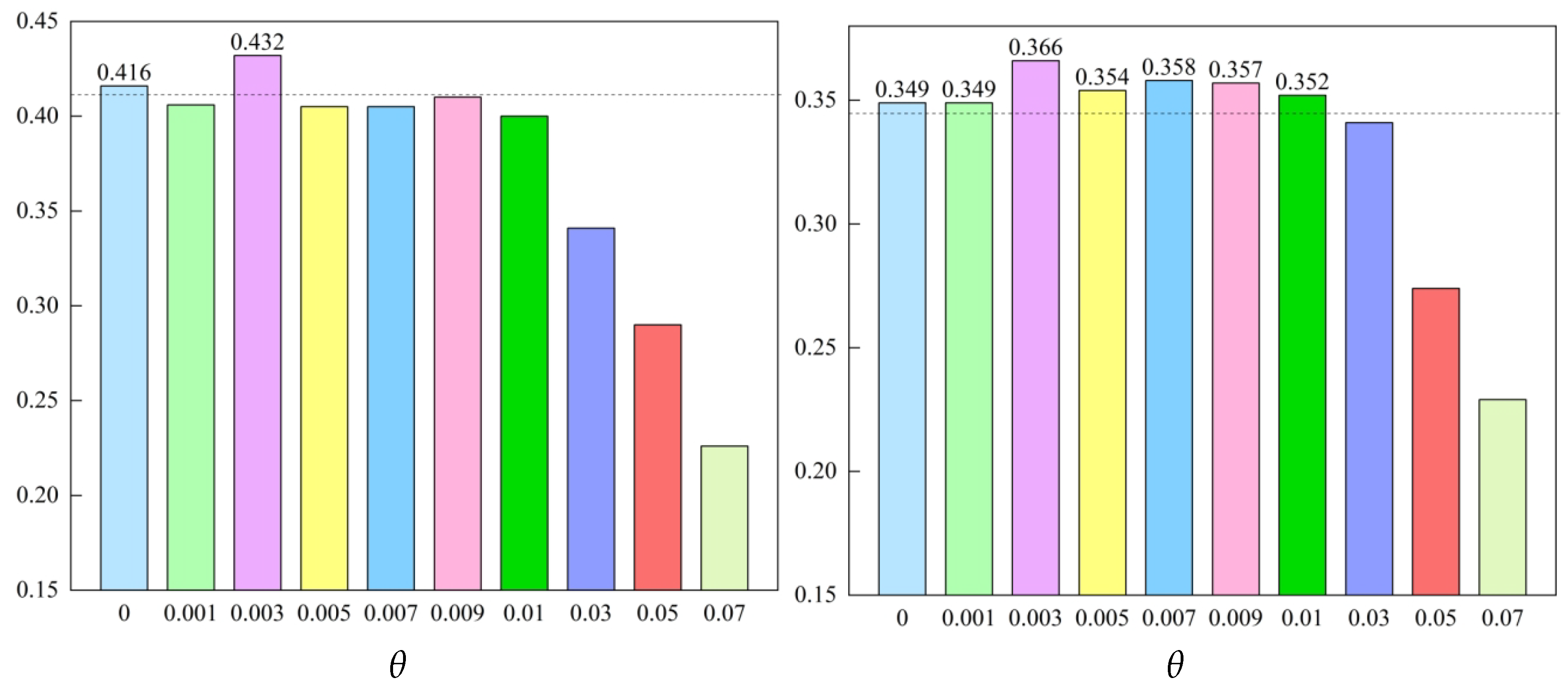
From Table 12 and Table 13, it is evident that different values of the hyperparameter $\theta$ have varying effects on the server and client evaluation metrics. This fully demonstrates the effectiveness and rationale of considering both the number of client samples and training loss in the SAPAA-MMF algorithm. To intuitively determine the optimal value of the hyperparameter $\theta$, the average values of various metrics and the corresponding values of $\theta$ are illustrated in a bar chart, as shown in Figure 5.

Figure 5. Mean value of client evaluation indicators using different parameter values (The dashed line represents the mean of indicators that do not take into account client losses.).

From Figure 5, it is evident that different values of the parameter $\theta$ in the SAPAA-MMF algorithm result in varying effects on both client-side and server-side evaluations. In the server evaluation, when the parameter $\theta$ is set to 0.003, the average metric value is 0.416 higher compared to the case where client loss is not considered. In the client evaluation, when the parameter $\theta$ is set to 0.003, 0.005, 0.007, 0.009, or 0.01, the average metric value is higher than the baseline value of 0.349, where client loss is not considered. Therefore, when the parameter $\theta$ is set to 0.003, the average evaluation metrics for both server and client are higher than those that do not consider client loss, achieving the best performance. This fully verifies that incorporating client loss during model parameter aggregation yields better results. Based on this analysis, the optimal value of $\theta$ used throughout this study is 0.003.

4.6. Validation of Multi-Method Fusion

This paper proposes the SAPAA-MMF algorithm. By leveraging the concept of multi-method fusion, different algorithms are combined, fully utilizing their complementary advantages to enhance the performance and generalization ability of the model while ensuring stability and convergence. To comprehensively verify the effectiveness of multi-method fusion, the FedAdam algorithm and the SAPAA-MMF algorithm without fusion are tested on five datasets. The detailed server and client evaluation metrics are presented in Table 14 and Table 15.

Table 14. Comparison between non-multi-method fusion and multi-method fusion server evaluation based on different datasets.

Dataset	No Fusion					Fusion ($\mathit{\theta }=0$)
	$\mathit{AP}$	${\mathit{AP}}_{\mathbf{50}}$	${\mathit{AP}}_{\mathbf{75}}$	${\mathit{AR}}_{\mathbf{100}}$	${\mathit{AR}}_{\mathbf{300}}$	$\mathit{AP}$	${\mathit{AP}}_{\mathbf{50}}$	${\mathit{AP}}_{\mathbf{75}}$	${\mathit{AR}}_{\mathbf{100}}$	${\mathit{AR}}_{\mathbf{300}}$
Bird’s nest foreign bodies	0.174	0.506	0.063	0.247	0.247	0.190	0.491	0.084	0.255	0.255
Cement rod damage	0.602	0.776	0.752	0.604	0.604	0.614	0.792	0.752	0.642	0.642
Shockproof hammer slip	0.438	0.703	0.521	0.521	0.534	0.442	0.708	0.559	0.549	0.549
Insulator self-explosion	0.330	0.517	0.407	0.370	0.376	0.341	0.525	0.404	0.390	0.391
Mixed	0.332	0.628	0.365	0.368	0.368	0.335	0.624	0.339	0.390	0.390
$Average$	0.375	0.626	0.422	0.422	0.426	0.384	0.628	0.428	0.445	0.445

Table 15. Comparison between non-multi-method fusion and multi-method fusion client evaluation based on different datasets.

Dataset	No Fusion					Fusion ($\mathit{\theta }=0$)
	$\mathit{AP}$	${\mathit{AP}}_{\mathbf{50}}$	${\mathit{AP}}_{\mathbf{75}}$	${\mathit{AR}}_{\mathbf{100}}$	${\mathit{AR}}_{\mathbf{300}}$	$\mathit{AP}$	${\mathit{AP}}_{\mathbf{50}}$	${\mathit{AP}}_{\mathbf{75}}$	${\mathit{AR}}_{\mathbf{100}}$	${\mathit{AR}}_{\mathbf{300}}$
Bird’s nest foreign bodies	0.214	0.564	0.140	0.281	0.282	0.232	0.573	0.160	0.285	0.285
Cement rod damage	0.564	0.853	0.703	0.631	0.631	0.603	0.850	0.742	0.655	0.656
Shockproof hammer slip	0.436	0.707	0.506	0.523	0.523	0.467	0.763	0.498	0.548	0.548
Insulator self-explosion	0.318	0.539	0.344	0.366	0.370	0.327	0.554	0.387	0.376	0.377
Mixed	0.265	0.537	0.238	0.334	0.334	0.284	0.539	0.271	0.326	0.326
$Average$	0.359	0.640	0.387	0.427	0.428	0.383	0.656	0.412	0.438	0.438

From Table 14 and Table 15, it is evident that after multi-method fusion, server-side evaluations showed improvements across multiple datasets. On the Bird’s Nest Foreign Bodies dataset, $AP$, $A{P}_{75}$, $A{R}_{100}$, and $A{R}_{300}$ increased by 1.6%, 2.1%, 0.8%, and 0.8%, respectively. On the Cement Pole Damage dataset, $AP$, $A{P}_{50}$, $A{R}_{100}$, and $A{R}_{300}$ increased by 1.2%, 1.6%, 3.8%, and 3.8%. On the Shockproof Hammer Slip dataset, $AP$, $A{P}_{50}$, $A{P}_{75}$, $A{R}_{100}$, and $A{R}_{300}$ increased by 0.4%, 0.5%, 3.8%, 2.8%, and 1.5%, respectively. On the Insulator Self-Explosion dataset, $AP$, $A{P}_{50}$, $A{R}_{100}$, and $A{R}_{300}$ increased by 1.1%, 0.8%, 2%, and 1.5%, respectively. On the mixed dataset, $AP$, $A{R}_{100}$, and $A{R}_{300}$ increased by 0.3%, 2.2%, and 2.2%.

In the client evaluation on the Bird’s Nest Foreign Bodies dataset, $AP$, $A{P}_{50}$, $A{P}_{75}$, $A{R}_{100}$, and $A{R}_{300}$ increased by 1.8%, 0.9%, 2%, 0.4%, and 0.3%, respectively. On the Cement Pole Damage dataset, $AP$, $A{P}_{75}$, $A{R}_{100}$, and $A{R}_{300}$ increased by 3.9%, 3.9%, 2.4%, and 2.5%, respectively. On the Shockproof Hammer Slip dataset, $AP$, $A{P}_{50}$, $A{R}_{100}$, and $A{R}_{300}$ increased by 3.1%, 5.6%, 2.5%, and 2.5%, respectively. On the Insulator Self-Explosion dataset, $AP$, $A{P}_{50}$, $A{P}_{75}$, $A{R}_{100}$, and $A{R}_{300}$ increased by 0.9%, 1.5%, 4.3%, 1%, and 0.7%, respectively. On the mixed dataset, $AP$, $A{P}_{50}$, and $A{P}_{75}$ increased by 1.9%, 0.2%, and 3.3%, respectively.

From both server-side and client-side evaluations, fully considering the stability of client data samples and utilizing adaptive aggregation during server-side parameter aggregation leads to better aggregation outcomes. This demonstrates that multi-method fusion effectively leverages the complementary strengths of different algorithms, significantly improving model performance and effectiveness.

4.7. Training Effectiveness Experiment

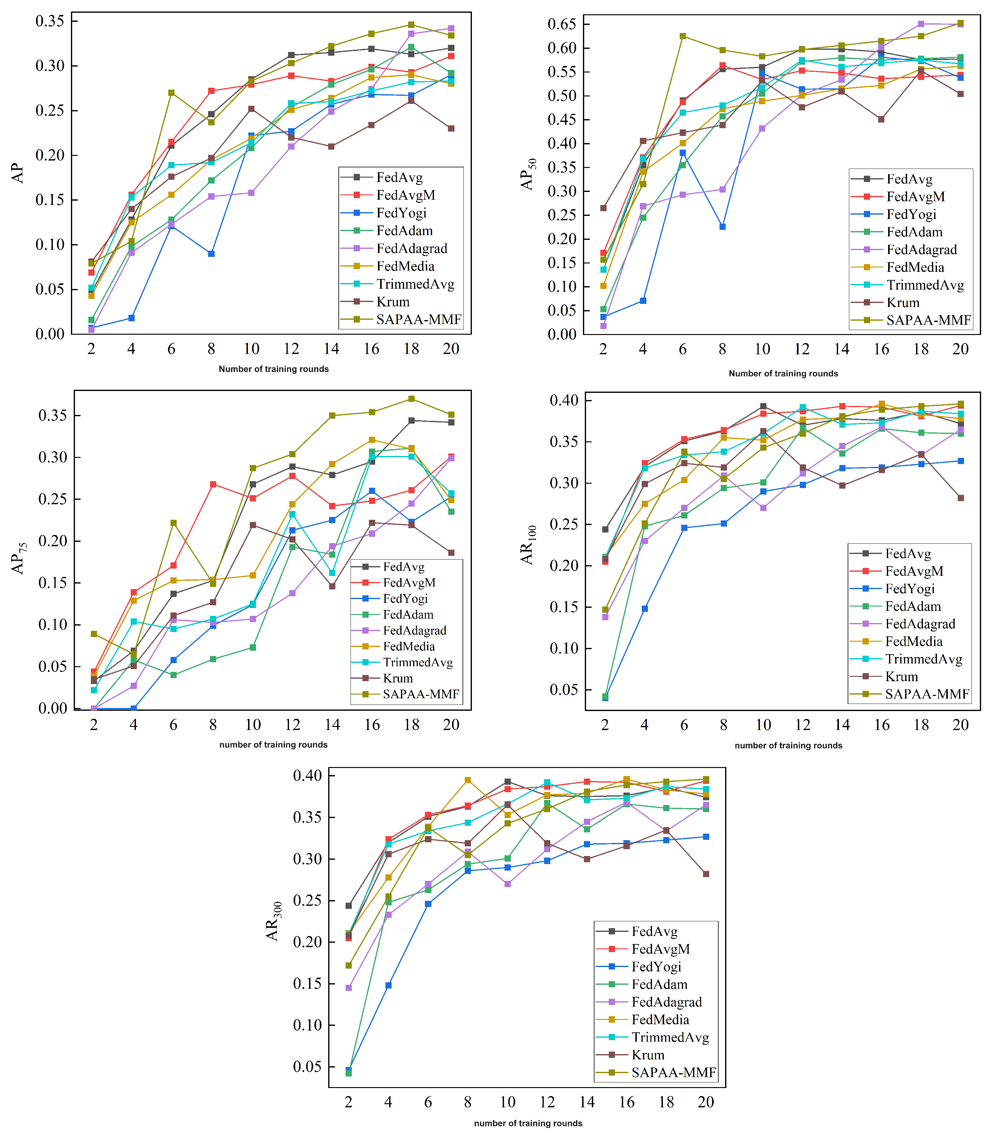
To verify the effectiveness of applying federated learning to the training of transmission line defect detection models and to assess the effectiveness of the constructed federated learning training framework, nine federated learning algorithms, including the SAPAA-MMF algorithm proposed in this chapter, were selected for evaluation in this section. Figure 6 illustrates the trends of various evaluation metrics ($AP$, $A{P}_{50}$, $A{P}_{75}$, $A{R}_{100}$, and $A{R}_{300}$) for SAPAA-MMF and other algorithms on the mixed dataset as training progresses. As shown in the figure, SAPAA-MMF and the other algorithms exhibit an upward trend in all five evaluation metrics as training progresses, eventually stabilizing after a certain point, demonstrating the good convergence ability of SAPAA-MMF. Furthermore, except for the $AP$ metric, where SAPAA-MMF is sub-optimal, SAPAA-MMF achieves the best results in the other four evaluation metrics after 20 training rounds, further demonstrating its effectiveness.

Figure 6. Evaluation metrics change curves for SAPAA-MMF and comparison algorithms run for 20 rounds on a mixed dataset.

4.8. Statistical Hypothesis Testing

The Friedman statistical test is a non-parametric method for comparing multiple related samples. It evaluates whether there are significant differences across conditions by ranking observed values and comparing the differences between these rankings. In this section, the Friedman test is used to conduct hypothesis testing to determine whether there are significant differences in the performance of each algorithm. The first step involves sorting all algorithms according to performance indicators for each dataset and assigning ranks from 1 to k. Next, the average ranking of each algorithm across all datasets is calculated. Finally, the statistics required for the test are calculated using Equations (23) and (24) as follows:

$${\tau }_{{\chi }^2}={\displaystyle \frac{12N}{k(k+1)}}\left(\sum _{i=1}^k{r}_i^2-{\displaystyle \frac{k{(k+1)}^2}{4}}\right),$$

(23)

$${\tau }_F={\displaystyle \frac{(N-1){\tau }_{{\chi }^2}}{N(k-1)-{\tau }_{{\chi }^2}}}.$$

(24)

where k is the number of algorithms participating in the statistical test, N is the number of datasets, and $r_i$ represents the average ranking value of the i algorithm in all datasets. ${\tau }_{{\chi }^2}$ is used to measure the ranking difference among algorithms and ${\tau }_F$ is the conversion of ${\tau }_{{\chi }^2}$ to make it obey the approximate normal distribution, which is used to further analyze that the ranking difference ${\tau }_F$ obeys the F distribution with degrees of freedom of $(k-1)$ and $(k-1)(N-1)$.

The significance level $\alpha$ is typically set at 0.05 in hypothesis testing. The null hypothesis posits that “there is no significant difference in the performance of the algorithms between the server and the client”. If the value of ${\tau }_F$ is less than the critical value of the F distribution at the significance level $\alpha$, the null hypothesis is accepted, indicating no significant difference in the performance of the algorithms between the server and the client. Otherwise, the null hypothesis is rejected, indicating a significant difference in performance.

To examine the performance differences between the server and the client across the nine algorithms, the Friedman statistical test was applied to analyze the experimental results. All statistical tests were conducted on the $AP$ metric. The experiment involved five datasets and nine algorithms. According to Equations (23) and (24), the value of $\tau F$ for the server evaluation is 19.38, and for the client evaluation it is 16.17. The critical value of the F distribution at a significance level of 0.05 is $F0.05(8,32)=2.244$. Since $19.38>2.244$ and $16.17>2.244$, the null hypothesis is rejected, indicating a significant difference in the performance of the algorithms between the server and the client. Based on these experimental results, it can be concluded that SAPAA-MMF outperforms the other comparison algorithms.

5. Conclusions

This study proposes a server-side Adaptive Parameter Aggregation Algorithm based on Multi-method Fusion (SAPAA-MMF) for transmission line defect detection. A federated learning framework for transmission line defect detection was constructed to enable distributed model training without the need to centrally store or transmit original data, addressing the issues of data silos, privacy concerns, and hardware performance limitations associated with traditional transmission line defect detection model training. To address the limitation that existing federated learning algorithms only use a single algorithm for server-side parameter aggregation, making it challenging to fully leverage the advantages of different algorithms, this study proposes a server-side adaptive parameter aggregation algorithm based on multi-method fusion to enhance the aggregation effect, model performance, and generalization ability. The performance of the SAPAA-MMF algorithm was compared with multiple baseline algorithms across five datasets, and the effectiveness of SAPAA-MMF was verified. This comprehensive performance across multiple datasets underscores the effectiveness of SAPAA-MMF in addressing challenges associated with federated learning in defect detection tasks. By integrating multiple methods and carefully balancing key factors, SAPAA-MMF demonstrates its capacity to provide a more reliable and adaptable solution for real-world transmission lines defect detection applications.

However, existing federated learning algorithms often overlook personalized client feature information during the client update process. Additionally, the generalization ability of these models for performing defect detection tasks in other domains has not been thoroughly demonstrated. Future research should explore additional strategies and optimize client parameter updates to further enhance model performance. Furthermore, applying SAPAA-MMF to defect detection tasks in other real-world scenarios could further highlight the effectiveness of our research approach.

References

- Miao, X.; Liu, X.; Chen, J.; Zhuang, S.; Fan, J.; Jiang, H. Insulator detection in aerial images for transmission line inspection using single shot multibox detector. IEEE Access 2019, 7, 9945–9956. [Google Scholar] [CrossRef] [Scilit]
- Zhao, Z.; Zhen, Z.; Zhang, L.; Qi, Y.; Kong, Y.; Zhang, K. Insulator detection method in inspection image based on improved faster r-cnn. Energies 2019, 12, 1204. [Google Scholar] [CrossRef] [Scilit]
- Feng, Z.; Guo, L.; Huang, D.; Li, R. Electrical insulator defects detection method based on yolov5. In Proceedings of the 2021 IEEE 10th Data Driven Control and Learning Systems Conference, Suzhou, China, 14–16 May 2021; pp. 979–984. [Google Scholar]
- Ju, M.; Yoo, C.D. Detection of bird’s nest in real time based on relation with electric pole using deep neural network. In Proceedings of the 2019 34th International Technical Conference on Circuits/Systems, Computers and Communications, Jeju, Republic of Korea, 23–26 June 2019; pp. 1–4. [Google Scholar]
- Zhang, C.; Xie, Y.; Bai, H.; Yu, B.; Li, W.; Gao, Y. A survey on federated learning. Knowl.-Based Syst. 2021, 216, 106775. [Google Scholar] [CrossRef] [Scilit]
- McMahan, B.; Moore, E.; Ramage, D.; Hampson, S.; Arcas, B.A.Y. Communication-efficient learning of deep networks from decentralized data. In Proceedings of the 20th International Conference on Artificial Intelligence and Statistics, Fort Lauderdale, FL, USA, 20–22 April 2017; pp. 1273–1282. [Google Scholar]
- Li, L.; Fan, Y.; Tse, M.; Lin, K.-Y. A review of applications in federated Learning. Comput. Ind. Eng. 2020, 149, 106854. [Google Scholar] [CrossRef] [Scilit]
- Hong, J.; Zhu, Z.; Yu, S.; Wang, Z.; Dodge, H.H.; Zhou, J. Federated adversarial debiasing for fair and transferable representations. In Proceedings of the 27th ACM SIGKDD Conference on Knowledge Discovery & Data Mining, Virtual Event, 14–18 August 2021; pp. 617–627. [Google Scholar]
- Karimireddy, S.P.; Kale, S.; Mohri, M.; Reddi, S.; Stich, S.; Suresh, A.T. Scaffold: Stochastic controlled averaging for federated learning. In Proceedings of the International Conference on Machine Learning, Virtual Event, 13–18 July 2020; pp. 5132–5143. [Google Scholar]
- Yuan, H.; Zaheer, M.; Reddi, S. Federated composite optimization. In Proceedings of the 38th International Conference on Machine Learning, Virtual Event, 18–24 July 2021; pp. 12253–12266. [Google Scholar]
- Reddi, S.; Charles, Z.; Zaheer, M.; Garrett, Z.; Rush, K.; Konečnỳ, J.; Kumar, S.; McMahan, H.B. Adaptive federated optimization. arXiv 2020, arXiv:2003.00295. [Google Scholar]
- Wu, Q.; An, J. An active contour model based on texture distribution for extracting inhomogeneous insulators from aerial images. IEEE Trans. Geosci. Remote Sens. 2013, 52, 3613–3626. [Google Scholar] [CrossRef] [Scilit]
- Wang, W.; Wang, Y.; Han, J.; Liu, Y. Recognition and drop-off detection of insulator based on aerial image. In Proceedings of the 2016 9th International Symposium on Computational Intelligence and Design, Hangzhou, China, 10–11 December 2016; pp. 162–167. [Google Scholar]
- Yan, S.; Jin, L.; Duan, S.; Zhao, L.; Yao, C.; Zhang, W. Power line image segmentation and extra matter recognition based on improved otsu algorithm. In Proceedings of the 2013 2nd International Conference on Electric Power Equipment-Switching Technology, Matsue, Japan, 20–23 October 2013; pp. 1–4. [Google Scholar]
- Chen, J.; Wen, Y.; Nanehkaran, Y.A.; Zhang, D.; Zeb, A. Multiscale attention networks for pavement defect detection. IEEE Trans. Instrum. Meas. 2023, 72, 1–12. [Google Scholar] [CrossRef] [Scilit]
- Yu, Y.; He, Y.; Karimi, H.R.; Gelman, L.; Cetin, A.E. A two-stage importance-aware subgraph convolutional network based on multi-source sensors for cross-domain fault diagnosis. Neural Netw. 2024, 179, 106518. [Google Scholar] [CrossRef] [Scilit] [PubMed]
- LeCun, Y.; Bengio, Y.; Hinton, G. Deep learning. Nature 2015, 521, 436–444. [Google Scholar] [CrossRef] [Scilit] [PubMed]
- Li, F.; Xin, J.; Chen, T.; Xin, L.; Wei, Z.; Li, Y.; Zhang, Y.; Jin, H.; Tu, Y.; Zhou, X.; et al. An automatic detection method of bird’s nest on transmission line tower based on faster_rcnn. IEEE Access 2020, 8, 164214–164221. [Google Scholar] [CrossRef] [Scilit]
- Li, L.; Wang, Z.; Zhang, T. Gbh-yolov5: Ghost convolution with bottleneckcsp and tiny target prediction head incorporating yolov5 for pv panel defect detection. Electronics 2023, 12, 561. [Google Scholar] [CrossRef] [Scilit]
- Wang, X.; Gao, H.; Jia, Z.; Li, Z. Bl-yolov8: An improved road defect detection model based on yolov8. Sensors 2023, 23, 8361. [Google Scholar] [CrossRef] [Scilit] [PubMed]
- Blanchard, P.; El Mhamdi, E.M.; Guerraoui, R.; Stainer, J. Machine learning with adversaries: Byzantine tolerant gradient descent. Adv. Neural Inf. Process. Syst. 2017, 30, 119–129. [Google Scholar]
- Yin, D.; Chen, Y.; Kannan, R.; Bartlett, P. Byzantine-robust distributed learning: Towards optimal statistical rates. In Proceedings of the 35th International Conference on Machine Learning, Stockholm, Sweden, 10–15 July 2018; pp. 5650–5659. [Google Scholar]
- Pan, Z.; Geng, H.; Wei, L.; Zhao, W. Adaptive client model update with reinforcement learning in synchronous federated learning. In Proceedings of the 2022 32nd International Telecommunication Networks and Applications Conference, Wellington, New Zealand, 30 November–2 December 2022; pp. 1–3. [Google Scholar]
- Li, T.; Sahu, A.K.; Zaheer, M.; Sanjabi, M.; Talwalkar, A.; Smith, V. Federated optimization in heterogeneous networks. Proc. Mach. Learn. Syst. 2020, 2, 429–450. [Google Scholar]
- Li, Q.; He, B.; Song, D. Model-contrastive federated learning. In Proceedings of the IEEE/CVF Conference on Computer Vision and Pattern Recognition, Nashville, TN, USA, 20–25 June 2021; pp. 10713–10722. [Google Scholar]
- Zhu, Z.; Hong, J.; Zhou, J. Data-free knowledge distillation for heterogeneous federated learning. In Proceedings of the 38th International Conference on Machine Learning, Virtual Event, 18–24 July 2021; pp. 12878–12889. [Google Scholar]
- Fallah, A.; Mokhtari, A.; Ozdaglar, A. Personalized federated learning with theoretical guarantees: A model-agnostic meta-learning approach. Adv. Neural Inf. Process. Syst. 2020, 33, 3557–3568. [Google Scholar]
- Li, X.-C.; Zhan, D.-C.; Shao, Y.; Li, B.; Song, S. Fedphp: Federated personalization with inherited private models. In Joint European Conference on Machine Learning and Knowledge Discovery in Databases; Springer: Cham, Switzerland, 2021; pp. 587–602. [Google Scholar]
- Chen, J.; Zhang, R.; Guo, J.; Fan, Y.; Cheng, X. Fedmatch: Federated learning over heterogeneous question answering data. In Proceedings of the 30th ACM International Conference on Information & Knowledge Management, Virtual Event, 1–5 November 2021; pp. 181–190. [Google Scholar]
- Niu, Y.; Deng, W. Federated learning for face recognition with gradient correction. In Proceedings of the AAAI Conference on Artificial Intelligence, Vancouver, BC, Canada, 28 February–1 March 2022; pp. 1999–2007. [Google Scholar]
- Collins, L.; Hassani, H.; Mokhtari, A.; Shakkottai, S. Exploiting shared representations for personalized federated learning. In Proceedings of the 38th International Conference on Machine Learning, Virtual Event, 18–24 July 2021; pp. 2089–2099. [Google Scholar]
- Shen, T.; Zhang, J.; Jia, X.; Zhang, F.; Lv, Z.; Kuang, K.; Wu, C.; Wu, F. Federated mutual learning: A collaborative machine learning method for heterogeneous data, models, and objectives. Front. Inf. Technol. Electron. Eng. 2023, 24, 1390–1402. [Google Scholar] [CrossRef] [Scilit]
- Shi, C.; Shen, C.; Yang, J. Federated multi-armed bandits with personalization. In Proceedings of the 24th International Conference on Artificial Intelligence and Statistics, Virtual Event, 13–15 April 2021; pp. 2917–2925. [Google Scholar]
- Kingma, D.P.; Ba, J. Adam: A method for stochastic optimization. arXiv 2014, arXiv:1412.6980. [Google Scholar]
- Hsu, T.-M.H.; Qi, H.; Brown, M. Federated visual classification with real-world data distribution. In Computer Vision–ECCV 2020: 16th European Conference, Glasgow, UK, 23–28 August 2020, Proceedings, Part X 16; Springer: Berlin/Heidelberg, Germany, 2020; pp. 76–92. [Google Scholar]
- Lin, T.-Y.; Maire, M.; Belongie, S.J.; Hays, J.; Perona, P.; Ramanan, D.; Dollár, P.; Zitnick, C.L. Microsoft coco: Common objects in context. In European Conference on Computer Vision; Springer: Berlin/Heidelberg, Germany, 2014; pp. 740–755. [Google Scholar]
Disclaimer/Publisher’s Note: The statements, opinions and data contained in all publications are solely those of the individual author(s) and contributor(s) and not of MDPI and/or the editor(s). MDPI and/or the editor(s) disclaim responsibility for any injury to people or property resulting from any ideas, methods, instructions or products referred to in the content. |
© 2024 by the authors. Licensee MDPI, Basel, Switzerland. This article is an open access article distributed under the terms and conditions of the Creative Commons Attribution (CC BY) license (https://creativecommons.org/licenses/by/4.0/).