Benchmarking LLM-Based Time-Series Foundation Models for Minute-Resolution Turning-Movement Traffic Dynamics on an Urban Arterial

Abstract

Large language models (LLMs) and time-series foundation models have advanced traffic forecasting, but almost exclusively on freeway sensors at five-minute, aggregate-flow resolution; their behavior on minute-resolution, movement-level counts at signalized arterials is unknown. This study assembled a real corridor dataset—6449 gap-free one-minute turning-movement records (255,364 counted vehicles) at 20 signalized intersections along 13 miles of Nolensville Pike, Nashville, Tennessee—and ran a controlled benchmark across three model families (classical, deep, and LLM/foundation models). We evaluate in-sample accuracy at 5/10/15 min horizons (RQ1), cross-date leave-intersection-out transfer to morning-only sites (RQ2). On the full-day sites, a per-series ARIMA attains the best short-horizon accuracy (MASE 0.87 at h = 5), while a zero-shot foundation model (Chronos) is the most stable across horizons; under leave-intersection-out transfer the ordering reverses—foundation models transfer best (MASE ≈ 0.61, improving to ≈0.56 with few-shot adaptation) whereas globally trained deep networks fail catastrophically (MASE > 4). All benchmark values reported here are measured on the corridor data; foundation-model families that we could not execute end-to-end in this environment are discussed qualitatively and are not included in the quantitative comparison. The dataset and protocol establish an honest, cost-aware basis for judging whether language and foundation models genuinely forecast an urban corridor at minute resolution.

1. Introduction

1.1. Motivation

Signalized urban arterials are among the most operationally demanding elements of the road network [1]. On a single corridor, dozens of signalized intersections interact through progression, queue spillback, and demand that rises and falls sharply within minutes of the peak. Turning-movement counts (TMCs)—the directional, per-movement tallies of vehicles at an intersection—are the fundamental measurement used to design signal timing, size turn lanes, estimate delay, and calibrate microsimulation models. Historically, TMCs are reported in coarse 15 min bins because manual counting and conventional detectors cannot reliably resolve finer intervals [2]. The recent proliferation of computer-vision-based collection platforms, such as Miovision, has changed this: video-derived counts can now be reported at 1 min resolution across an entire corridor, exposing the minute-scale demand structure that 15 min aggregation deliberately smooths away [3]. This resolution creates both an opportunity and a modeling challenge—short-horizon fluctuations at the movement level are highly variable (“bursty”), yet they carry information directly relevant to adaptive signal control and real-time operations.

In parallel, a rapid and somewhat surprising development has taken place in the machine-learning literature: large language models (LLMs) and, more broadly, transformer-based time-series foundation models (TSFMs) are being repurposed for numerical forecasting tasks well outside natural language [4,5,6]. The central claim of this line of work is that a model pretrained on massive sequence corpora learns general-purpose representations of temporal structure that transfer, with little or no task-specific training, to unseen forecasting problems [7,8]. If that claim holds for traffic, it would be consequential for transportation agencies: a single pretrained model could, in principle, produce short-horizon forecasts at intersections where little or no historical data exists—precisely the situation at most arterials, where instrumented counts are collected for only a few hours on a single day. Yet the evidence for LLMs in traffic remains thin and, importantly, contested. Purpose-built spatio-temporal LLM adaptations such as ST-LLM [9,10], ST-LLM+ [11], and LEAF [12] report state-of-the-art accuracy on widely used sensor benchmarks (e.g., the PEMS freeway loop-detector datasets). At the same time, a rigorous ablation study has shown that, for several published LLM forecasters, removing the language-model backbone entirely—or replacing it with a single attention layer—does not degrade, and sometimes improves, accuracy [13]. This tension motivates careful, application-specific benchmarking rather than uncritical adoption. Crucially, essentially all of the traffic evidence to date concerns freeway mainline sensors at 5 min resolution; the behavior of these models on minute-resolution, movement-level, signalized-arterial data—where the target is a small, noisy, integer count for a specific turning movement—has not been established.

1.2. The Gap

We identify two specific gaps in the literature that this study addresses. First, a resolution and target-granularity gap [14]. LLM and TSFM traffic studies overwhelmingly forecast aggregate directional flow on freeway detectors at 15 min (or coarser sometimes) resolution [9,11,12]. Arterial operations, however, are governed by individual turning movements (through, left, right) at each approach, and emerging sensing supports 1 min reporting. Minute-level movement counts are far sparser and burstier than freeway flow, and it is unknown whether foundation models—whose advantage is often attributed to learning smooth, periodic structure—retain any benefit in this regime. Second, a transfer/data-scarcity gap. The practical appeal of a pretrained model is zero- or few-shot deployment where historical data is unavailable [7,8]. Real corridor data collection is intermittent: different intersections are counted on different days, for different durations, using portable equipment. Whether a model trained on the handful of intersections with long (all-day) counts can transfer to intersections observed for only a few morning hours—and to unseen dates—is exactly the question an agency would ask, yet it is rarely evaluated under realistic, non-synchronized collection conditions.

1.3. Study Design and Contributions

To address these gaps we assemble and analyze a real, minute-resolution corridor dataset: 1 min turning-movement counts collected with Miovision equipment at 20 signalized intersections along a 13-mile section of Nolensville Pike in Nashville, Tennessee, spanning from Concord Road in the south to the Lafayette Street/4th Avenue South terminus in the north. The dataset comprises 6449 one-minute observations, each recording sixteen movements (four approaches × {right, through, left, U-turn}). Six intersections were counted for a full day (approximately 6 A.M.–6 P.M.); the remaining fourteen were counted over roughly three-hour windows concentrated in the A.M. peak (mostly 7–10 A.M.). Because each site was counted on a different date, the corridor is deliberately treated in relative and clock-aligned time rather than as a synchronized snapshot—a realistic and, as we argue, methodologically important framing for the transfer experiments. Against this testbed we conduct a controlled benchmark that spans three model families: (i) classical statistical forecasters (seasonal-naïve, ARIMA/SARIMA, exponential smoothing) [2,15]; (ii) deep sequence models (LSTM and the Temporal Fusion Transformer, TFT [16]); and (iii) LLM- and foundation-model-based forecasters, including frozen-backbone LLM adapters [5,6], time-series foundation models using zero-shot [7,8], and a spatio-temporal LLM configuration in the spirit of ST-LLM [9]. We organize the evaluation around three research questions:

• RQ1 (Accuracy). How do LLM/TSFM forecasters compare to classical and deep baselines for 5, 10, and 15 min ahead prediction of directional and turning-movement flow at minute resolution?
• RQ2 (Transfer). Can a model trained on the long-count intersections generalize, in few-shot and zero-shot settings, to intersections observed only during the A.M. peak and to unseen dates—i.e., does pretraining confer a corridor-transfer advantage under realistic data scarcity?

The contributions are threefold. (1) We introduce, to our knowledge, the first benchmark of LLM and time-series foundation models on minute-resolution, movement-level signalized-arterial data, complementing the freeway-sensor focus of prior work [9,11,12]. (2) We evaluate model transfer under a realistic non-synchronized collection protocol that mirrors how agencies actually gather corridor data. (3) We report an honest cost–accuracy accounting, quantifying where the language-model machinery earns its computational expense against strong, inexpensive baselines [13]—a comparison the recent literature suggests is essential rather than optional. As a further direction, we specify (but leave to future work) a deterministically scored protocol for evaluating LLM-generated natural-language explanations of corridor dynamics.

1.4. Paper Organization

The remainder of the paper is organized as follows. Section 2 reviews related work on LLMs and foundation models for time-series and traffic forecasting, and on classical arterial modeling. Section 3 describes the Nolensville Pike corridor, the Miovision data collection, and the coverage and data-quality characteristics that shape our experimental design. Section 4 details the model families, prompt formulations, transfer protocol, and evaluation metrics. Section 5 presents results for RQ1 and RQ2. Section 6 discusses when and why the language-model approaches help, their computational cost, and their robustness to minute-scale burstiness. Section 7 concludes and outlines extensions.

2. Related Work

We organize prior work into four streams: (i) foundation models that adapt language-model architectures to general time-series forecasting; (ii) LLM- and foundation-model methods developed specifically for traffic prediction; (iii) the emerging critical literature that questions whether the language-model component actually contributes to forecasting skill; and (iv) classical and deep approaches to arterial and turning-movement analysis, which supply both our baselines and the operational framing of the problem. We then position the present study against these streams.

2.1. Language Models and Foundation Models for Time-Series Forecasting

The premise that a transformer trained at scale learns transferable temporal structure has produced two broad design patterns. The first repurposes a frozen, pretrained language model for numeric forecasting. Zhou et al. introduced the “One-Fits-All” Frozen Pretrained Transformer (GPT4TS), showing that leaving the self-attention and feed-forward blocks of a pretrained GPT-2 intact—while fine-tuning only lightweight input and output layers—yields competitive or state-of-the-art results across forecasting, classification, imputation, and anomaly-detection tasks [5]. Jin et al. extended this idea with Time-LLM, a reprogramming framework that maps input series into text-prototype representations and prepends a natural-language “Prompt-as-Prefix” so that an off-the-shelf LLM can reason about the series without altering its weights; the authors report strong few-shot and zero-shot performance and explicitly frame forecasting as “yet another language task” [6]. Both efforts trace their architectural lineage to the transformer [17]. The second pattern builds dedicated time-series foundation models (TSFMs) that borrow language-model training recipes but are trained from scratch on time-series corpora. TimesFM is presented as the first such foundation model, trained on more than one hundred billion data points and evaluated for zero-shot forecasting across diverse domains; notably, its authors emphasize that it is a transformer specialized for time series rather than a repurposed LLM [7,18]. Chronos takes a middle path: it tokenizes real-valued series via scaling and quantization into a fixed vocabulary and then trains standard language-model architectures (the T5 family) on these tokens with a cross-entropy objective, achieving zero-shot accuracy that matches or exceeds purpose-built models on dozens of benchmark datasets [8]. Collectively, this literature establishes the capabilities our study probes—transfer, few-shot/zero-shot inference, and prompt-based reasoning—while leaving open whether they survive at minute resolution on movement-level arterial counts.

2.2. LLMs and Foundation Models for Traffic Prediction

Within transportation, the adaptation of LLMs has accelerated rapidly. The recent survey by Mahmud et al. catalogs applications spanning autonomous driving, travel-behavior prediction, and general transportation queries, and identifies methodological patterns—zero-/few-shot learning, prompt engineering, and fine-tuning—together with open research gaps [4]. For network-level flow forecasting specifically, Liu et al. proposed ST-LLM, which treats the timesteps at each location as tokens, learns a spatio-temporal embedding, and applies a partially frozen attention strategy to adapt an LLM to capture spatial and temporal dependencies; they report state-of-the-art accuracy and, importantly for our RQ2, robust few-shot and zero-shot behavior on real traffic datasets [9,19]. The subsequent ST-LLM+ incorporates a proximity-based adjacency matrix and a partially frozen graph-attention module, with LoRA-based parameter-efficient fine-tuning, to better model localized network dependencies [11,18]. Zhao et al.’s LEAF takes a discriminative rather than generative route: two branches (graph and hypergraph) generate candidate forecasts, and a frozen LLM selects among them, with a ranking loss used to train the predictor—an approach reported to reach state-of-the-art results on the PEMS datasets [12,20]. A common thread runs through these traffic studies: they evaluate on freeway loop-detector benchmarks (predominantly the PEMS family) at five-minute resolution, and they forecast aggregate directional flow rather than individual turning movements. None, to our knowledge, addresses one-minute, movement-level counts on a signalized arterial, nor a realistic non-synchronized, multi-day collection protocol. This is the empirical space our benchmark occupies.

2.3. Do the Language Models Actually Help?

An essential counter-current tempers the enthusiasm above and directly motivates our cost–benefit framing. Tan et al. conducted systematic ablations on several popular LLM-based forecasters and found that removing the language-model backbone entirely—or replacing it with a single attention layer—did not degrade forecasting accuracy, and in a majority of dataset–metric combinations actually improved it [13]. Their conclusion, that pretraining on language corpora appears unnecessary for the forecasting tasks examined, does not deny that LLM-style architectures can forecast well; rather, it warns that reported gains may stem from components other than the pretrained language knowledge, and that strong, inexpensive baselines are frequently under-reported. We take this finding seriously by (a) including classical and lightweight deep baselines as first-class comparators rather than strawmen, and (b) reporting inference cost alongside accuracy, so that any advantage attributed to the language-model machinery is weighed against its computational price.

2.4. Classical and Deep Approaches to Arterial and Turning-Movement Analysis

The operational backbone of arterial analysis remains the turning-movement count and the delay/capacity procedures codified in the Highway Capacity Manual (HCM), which conventionally analyze demand in fifteen-minute peak periods and translate movement volumes into phasing, capacity, and level-of-service estimates [2]. These procedures define the practical quantities—directional and movement-level flow, peak-hour factor, and the peak fifteen minutes—that any forecasting model must ultimately serve, and they justify our choice of movement-level targets. On the sensing side, computer-vision platforms such as Miovision now enable nonintrusive, video-based collection of turning movements at fine temporal resolution, making one-minute reporting feasible and thereby exposing the minute-scale demand structure that motivates this study [3]. For predictive modeling, classical statistical methods—seasonal-naïve, autoregressive integrated moving average (ARIMA/SARIMA), and exponential smoothing—remain standard, interpretable baselines for short-horizon traffic forecasting and are the reference against which learned models must justify their complexity [2]. Among deep models, recurrent architectures (LSTM) and, more recently, attention-based multi-horizon forecasters, have become common [21]. The Temporal Fusion Transformer (TFT) of Lim et al. is particularly relevant here: it combines recurrent local processing with interpretable self-attention and specialized components for selecting relevant covariates, delivering strong multi-horizon accuracy while exposing interpretable temporal importance—properties well matched to arterial forecasting, where known covariates (time of day, upstream flow, intersection identity) are available [16]. We adopt LSTM and TFT as our deep baselines and evaluate the LLM/TSFM family against them. Graph-based spatio-temporal models such as DCRNN [22] and STGCN [23] established the network-level forecasting paradigm that arterial movement-level counts depart from [18,19,21].

2.5. Positioning of This Study

We transfer the capabilities established for freeway, five-minute, aggregate-flow forecasting to a previously unexamined regime: one-minute, movement-level, signalized-arterial counts along a single instrumented corridor. Then, the analysis adopts the discipline the critical literature calls for—strong baselines and explicit cost accounting—rather than assuming the language model helps. The paper then aligns our forecasting targets and evaluation with the operational quantities (movement flow, peak dynamics) that arterial practice actually uses. From the reviewed literature, this combination—minute-resolution movement-level arterial data, a realistic non-synchronized transfer protocol, and an honest accuracy–cost comparison across three model families—has not previously been reported.

3. Data

3.1. Study Corridor

The study corridor is an approximately 13-mile section of Nolensville Pike (US-31A/US-41A/SR-11) in Nashville, Tennessee, Table 1. The corridor extends from its southern gateway at the intersection with Concord Road (SR-253), near the Williamson–Davidson county line, northward to its downtown terminus in the vicinity of Lafayette Street and 4th Avenue South, where the arterial transitions into the one-way 4th Avenue South pair serving the central business district. Nolensville Pike is the principal north–south commuter artery for the southeastern Nashville metropolitan area, carrying inbound (northbound) commute demand toward downtown and Interstate 440 in the morning and the reverse movement in the afternoon. Along its length it intersects several major cross-street and interchange facilities—including Old Hickory Boulevard, Harding Place, Thompson Lane, and the I-440 ramps—that inject and withdraw substantial cross traffic, punctuated by numerous minor signalized and unsignalized intersections whose counts were not collected. Twenty signalized intersections were instrumented for this study. They are numbered 1–20 from south (Concord Road) to north (Lafayette Street/4th Avenue South), preserving the physical ordering along the corridor. This ordering is used throughout the paper so that spatial relationships—upstream/downstream adjacency, progression, and the correlation structure examined in Section 5—can be read directly from the intersection index. Because several intermediate signals were not counted, adjacent indices are near-neighbors rather than strictly contiguous signals; we account for this when interpreting spatial coupling.

Table 1. Data collection summary for the twenty intersections along Nolensville Pike (south to north).

#	Cross Street	Date	Window	Records (min)	Coverage	Total Veh.	NB	SB	EB	WB	Peak hr (Veh)	PHF
1	Concord Rd	30 March 2026	06:30–09:29	180	AM	5547	2892	1105	1088	462	1972	0.88
2	Holt Rd	27 April 2026	07:30–10:29	180	AM	4475	2150	1579	595	151	1737	0.91
3	Bienville Dr	31 March 2026	06:30–09:29	180	AM	3022	1573	1193	0	256	1078	0.86
4	Celebratory Way	1 April 2026	07:30–10:29	180	AM	4385	1867	1504	98	916	1671	0.87
5	Old Hickory Blvd	10 December 2025	07:11–16:38	568	12 h	32,425	6754	7707	8869	9095	4155	0.95
6	Brewer Dr	27 April 2026	06:30–09:29	180	AM	5687	2821	2455	234	177	2027	0.91
7	Tusculum Rd	23 March 2026	07:31–10:29	179	AM	6201	2855	2174	328	844	2234	0.88
8	Haywood Ln	23 March 2026	07:30–10:29	180	AM	7320	4081	2111	129	999	2801	0.88
9	Harding Pl	9 December 2025	06:31–18:12	702	12 h	36,771	12,400	8238	6542	9591	3611	0.94
10	Paragon Mills Rd	26 March 2026	07:30–10:29	180	AM	6641	3533	1996	98	1014	2346	0.93
11	Allied/Wheeler	26 March 2026	07:00–09:59	180	AM	5603	2788	2542	37	236	1959	0.94
12	Elgin St	9 April 2026	07:30–10:29	180	AM	6574	3560	2995	19	0	2337	0.92
13	Thompson Ln	20 January 2026	06:36–16:37	602	12 h	32,084	8154	6733	8830	8367	3909	0.94
14	Peachtree St	4 December 2025	06:19–18:03	705	12 h	29,578	10,459	13,350	4504	1265	2926	0.95
15	I-440 WB Ramp	3 December 2025	07:07–18:21	675	12 h	32,055	13,154	13,175	0	5726	3500	0.95
16	Glenrose Rd	24 March 2026	07:00–09:59	180	AM	1762	681	712	0	369	1762	0.89
17	Polk Ave	8 April 2026	07:30–10:29	180	AM	5934	2737	2049	0	1148	2176	0.92
18	Craighead St	8 April 2026	07:30–10:29	180	AM	4603	1970	1713	920	0	1725	0.85
19	4th Ave S/I-40 EB Ramp	6 April 2026	06:39–09:29	171	AM	4695	2	2344	2349	0	1865	0.93
20	4th Ave S/Lafayette St	19 November 2025	06:18–17:44	687	12 h	20,002	0	7071	7622	5309	2503	0.93

Note: A count of 2 NB vehicles at site 19 and 0 at site 20 reflect ramp/one-way geometry at the southern terminus, not missing data.

3.2. Data Collection

Turning-movement counts were collected using Miovision video-based equipment, a nonintrusive, computer-vision platform that classifies and tallies vehicles by approach and movement from recorded video [3]. Each observation reports counts for sixteen movements—the four approaches (northbound, southbound, eastbound, westbound) each disaggregated into right-turn, through, left-turn, and U-turn movements—at a temporal resolution of one minute. This is substantially finer than the fifteen-minute intervals conventional in arterial practice [2], and it is the defining characteristic of the dataset: it preserves the minute-scale demand structure that fifteen-minute aggregation removes. Collection was performed on a per-intersection basis over a five-month period (November 2025 through April 2026). Two collection regimes are present. Six intersections (Nos. 5, 9, 13, 14, 15, and 20) were counted over a full service day of roughly twelve hours (approximately 6 A.M. to 6 P.M.), capturing both the morning and afternoon peaks. The remaining fourteen intersections were counted over shorter windows of approximately three hours, concentrated in the morning peak and most commonly spanning 7:00–10:00 A.M. Critically, no more than two intersections were counted on the same date. This reflects the realities of portable, equipment-constrained field collection and has a direct methodological consequence: the corridor cannot be treated as a synchronized snapshot of simultaneous flows. We therefore analyze the corridor in relative (elapsed-from-start) and clock-aligned time, and we design the transfer experiments to exploit—rather than obscure—this non-synchronized structure.

3.3. Dataset Summary and Coverage

The assembled dataset contains 6449 one-minute observations totaling 255,364 counted vehicle-movements across the twenty intersections. Every intersection’s series is temporally complete: within each site’s collection window there are no missing minutes, so the one-minute series are gap-free and require no imputation. Table 1 summarizes, for each intersection, the collection date, start and end clock times, number of one-minute records, total counted volume, the directional decomposition, and two operational descriptors computed from the one-minute series: the observed peak-hour volume (the maximum count over any sixty consecutive minutes) and the corresponding peak-hour factor (PHF), defined as the peak-hour volume divided by four times the peak fifteen-minute count within that hour. Higher PHF values at the full-day, high-volume sites arise because larger sample volumes smooth the peak fifteen-minute ratio, whereas lower-volume minor approaches show more within-hour spikiness and thus lower PHFs. All values in Table 1 are computed directly from the one-minute records; NB/SB/EB/WB are total counted vehicles per approach; “Peak hr” is the maximum 60 min rolling volume; PHF is the peak-hour factor. From Table 1, NB/SB/EB/WB are total counted vehicles on each approach across the collection window. “Peak hr (veh)” is the maximum sixty-minute rolling volume; PHF is the peak-hour factor computed from the one-minute series. Coverage “AM” denotes an approximately three-hour morning window; “12 h” denotes an approximately twelve-hour full-day count. All values are computed directly from the one-minute records. Several features of Table 1 shape the analysis. Observed peak-hour factors are tightly clustered between 0.85 and 0.95, consistent with a mature urban arterial exhibiting sustained rather than sharply spiked peaking [2]; the six full-day sites tend toward the upper end (0.93–0.95), reflecting the smoothing effect of higher volumes. Total counted volumes span two orders of magnitude at the extremes—from a low of 1762 vehicles at the low-volume Glenrose Road minor intersection (No. 16) to 36,771 at Harding Place (No. 9), the busiest site—though the disparity is driven substantially by collection duration (three-hour versus twelve-hour windows) as well as by intrinsic demand. Two intersections at the downtown terminus, Nos. 19 and 20, record essentially zero northbound volume (2 and 0 vehicles, respectively); this is not missing data but a true reflection of the one-way 4th Avenue South configuration, where the northbound movement is carried on a parallel facility. These structural zeros are retained and flagged, because a forecasting or explanation model must not confuse a genuine structural zero with an unobserved value. Because total counted volume depends on collection duration, cross-site comparisons are made on duration-invariant quantities (directional shares and the peak-hour factor) rather than on absolute totals.

3.4. Corridor-Level Flow Characteristics

Aggregated across all twenty intersections, the corridor is strongly oriented along its north–south mainline. Structural-zero and near-zero movements (e.g., the effectively zero northbound volume at the downtown one-way sites Nos. 19 and 20) are retained in these corridor totals because they represent true observed absence of flow rather than missing data; excluding them changes the reported NB/SB shares by less than 0.1 percentage point. Northbound and southbound movements account for 84,431 (33.1%) and 82,746 (32.4%) counted vehicles, respectively, so that the mainline (NB + SB) represents 167,177 vehicles, or 65.5% of all counted movement, against 88,187 vehicles (34.5%) on the east–west cross-street approaches. The near-balance between northbound and southbound totals is an artifact of aggregating morning-dominant (northbound/inbound) three-hour sites with full-day sites that also capture the afternoon (southbound/outbound) peak; at the movement level within the morning window the inbound bias is pronounced. The composition by movement type is dominated, as expected on an arterial, by through movements. Corridor-wide, through movements comprise 172,029 counted vehicles (67.4%), right turns 44,046 (17.3%), and left turns 39,264 (15.4%); U-turns are operationally negligible at 25 vehicles (0.01%) across the entire dataset. The two mainline through movements alone—northbound through (62,652) and southbound through (67,019)—account for just over half of all counted vehicles, underscoring that corridor performance is governed primarily by the progression of these two movements through successive signals.

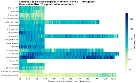
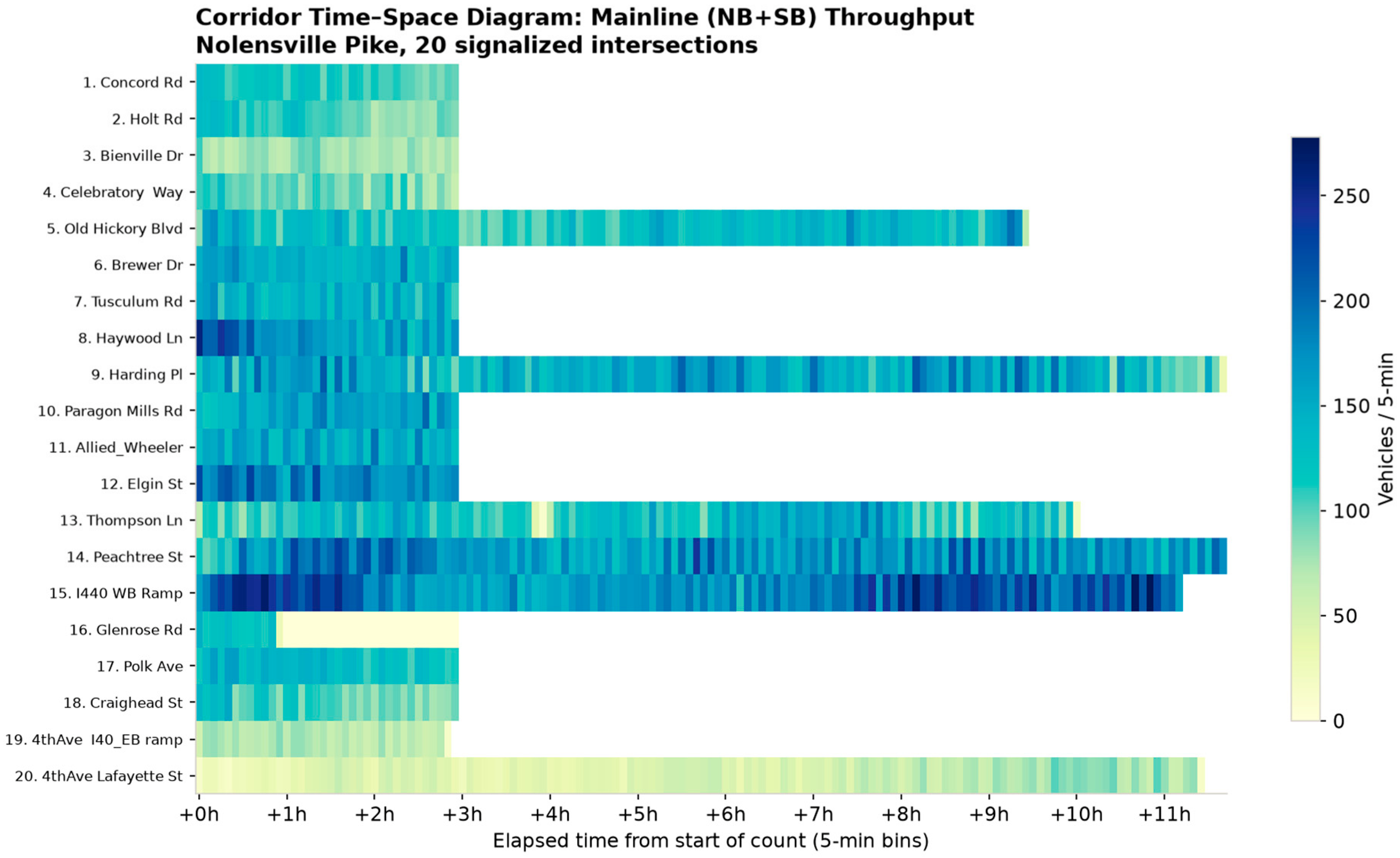
Figure 1 presents a time–space representation of the corridor’s mainline (northbound-plus-southbound) throughput. Each row corresponds to one intersection, ordered from south (No. 1, Concord Road, top) to north (No. 20, Lafayette Street, bottom); the horizontal axis is elapsed time measured from the start of each intersection’s own count, binned into five-minute intervals; and cell color encodes mainline vehicles per five-minute bin. Because collection dates and start times differ across sites, elapsed-time alignment is the appropriate common reference; the figure therefore depicts each site’s demand profile relative to its own observation window rather than a single synchronized clock. Clock-time alignment is not possible because no two sites share a collection date; elapsed-time alignment therefore compares each site at a like phase of its own demand profile, at the cost of not supporting claims about simultaneous corridor-wide behavior. Two structural facts are immediately legible. First, the two collection regimes are visually separated: fourteen rows terminate at roughly the three-hour mark (180 five-minute-bin columns ≈ 36 bins), while the six full-day sites (Nos. 5, 9, 13, 14, 15, 20) extend across the full ~11–12 h span. Second, the intensity structure reveals the corridor’s demand hierarchy. The heaviest sustained mainline throughput appears at the interchange-adjacent sites—most prominently the I-440 westbound ramp (No. 15) and Peachtree Street (No. 14), whose early-window cells reach the darkest band (on the order of 250+ mainline vehicles per five minutes)—and at Haywood Lane (No. 8), which shows an intense early-morning band before tapering. The full-day sites further reveal the afternoon re-intensification: Old Hickory Boulevard (No. 5), Harding Place (No. 9), and Thompson Lane (No. 13) each show a second high-throughput band in the afternoon portion of their rows, consistent with the corridor’s bidirectional commute role and with the fact that their observed peak hours fall in the afternoon (Table 1: 13:40–15:46). The low-volume minor intersection at Glenrose Road (No. 16) is visible as the palest row.

Figure 1. Mainline (NB + SB) throughput corridor time–space structure of mainline throughput.

3.5. Directional Composition and Turning-Movement Share

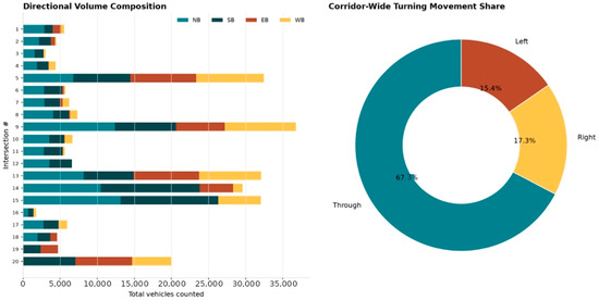
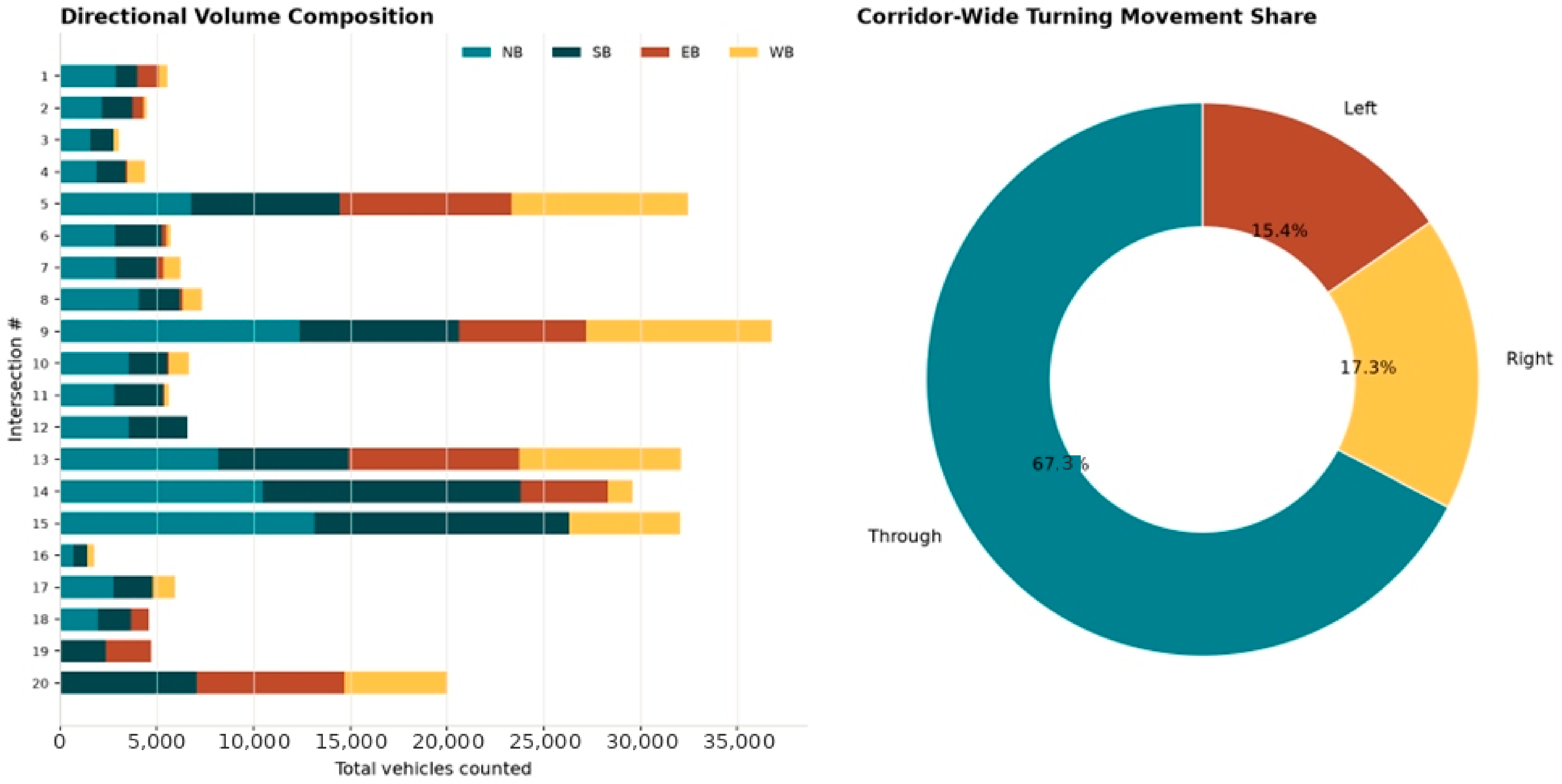
Figure 2 characterizes the corridor’s flow structure through two complementary panels. The left panel is a horizontal stacked bar chart giving, for each of the twenty intersections, the decomposition of total counted volume into its four directional approaches (NB, SB, EB, WB). The panel makes the corridor’s operational geography explicit. The mainline-dominated character of most sites appears as bars composed largely of the two mainline directions; the interchange and major-cross-street sites (Nos. 5, 9, 13) stand out both for their overall length—each exceeding 32,000 counted vehicles owing to full-day collection—and for their large east–west components, reflecting the heavy cross traffic these facilities carry. The terminus sites (Nos. 19 and 20) are visibly asymmetric, with negligible northbound contribution, a direct consequence of the one-way downtown configuration. Peachtree Street (No. 14) and the I-440 ramp (No. 15) show the largest mainline through-volumes, consistent with their role as the corridor’s highest-throughput segments. The right panel is a donut chart of corridor-wide turning-movement share, partitioning all counted vehicles into through (67.4%), right-turn (17.3%), and left-turn (15.4%) movements (U-turns, at 0.01%, are omitted from the visual for legibility). The dominance of through movement quantifies the corridor’s function as a mobility spine: roughly two of every three counted vehicles proceed straight through the intersection, so that the corridor’s level of service is governed primarily by the efficiency with which successive signals pass the mainline through movement. The remaining one-third of demand—turning traffic entering and leaving via cross streets—defines the exchange with the surrounding network and is the source of the block-to-block variation in mainline volume observed in Figure 2. Together, the two panels of Figure 2 establish the volumetric and directional context against which the per-movement forecasting targets.

Figure 2. Directional composition (NB/SB/EB/WB) of counted volume by intersection.

4. Methods

This section defines the forecasting task and its variants, the input representation and feature construction shared across models, the three model families under comparison and their configurations (summarized in Table 2), the prompt formulations used for the language-model forecasters, the training, validation, and transfer protocols that operationalize RQ1 and RQ2, and the evaluation metrics and statistical testing procedures.

Table 2. Models compared, by family, with key configuration.

Family	Model	Role	Trained Params	Covariates	Cross-Series	Key Hyperparameters
A—Classical	Seasonal-naïve	Reference floor	none	none	per-series	seasonal lag = target period
A—Classical	ARIMA/SARIMA	Statistical baseline	per-series	none	per-series	(p,d,q)(P,D,Q) by AIC search
A—Classical	ETS (exp. smoothing)	Statistical baseline	per-series	none	per-series	additive error + trend
B—Deep	LSTM enc–dec	Deep baseline	full	temporal + static	global	2 layers, hidden 128, dropout 0.1
B—Deep	Temporal Fusion Transformer [16]	Deep SOTA baseline	full	temporal + static + known-future	global	hidden 128, 4 attn heads, VSN on
C—LLM/TSFM	GPT4TS (frozen GPT-2) [5]	Frozen-LLM adapter	input/output only	temporal + static	global	GPT-2 backbone frozen; patch len 16
C—LLM/TSFM	Time-LLM (reprogrammed) [6]	Reprogrammed LLM	reprog. layers only	temporal + static + prompt prefix	global	frozen LLM backbone; text prototypes
C—LLM/TSFM	TimesFM [7]	Foundation model, zero-shot	none (zero-shot)	temporal (as supported)	pretrained	zero-shot + optional fine-tune variant
C—LLM/TSFM	Chronos [8]	Foundation model, zero-shot	none (zero-shot)	none (univariate)	pretrained	quantized tokens; probabilistic
C—LLM/TSFM	ST-LLM (spatio-temporal) [9]	Spatio-temporal LLM	partial (partly frozen attn)	temporal + static + upstream	global	timesteps-as-tokens; ST embedding

4.1. Problem Formulation

Let y^m_i(t) denote the count of movement m at intersection i during the one-minute interval ending at time t, where m ranges over the twelve non-U-turn movements (four approaches × {right, through, left}) and i ∈ {1,…,20}. U-turn movements are excluded from forecasting targets because they are operationally negligible (25 vehicles across the entire dataset). We consider three forecasting targets at increasing levels of aggregation, all derived from the same one-minute records:

• Movement-level flow y^m_i(t): The most granular and most challenging target, and the one most relevant to signal-phase design.
• Directional (approach) flow y^d_i(t) = Σ_m∈d y^m_i(t) for d ∈ {NB, SB, EB, WB}.
• Mainline through flow y^ML_i(t) = y^NBT_i(t) + y^SBT_i(t): The operationally dominant quantity governing progression.

Formally, at each forecast origin t we predict the next h one-minute movement counts y_{t + 1}, …, y_{t + h}; RQ1 evaluates h ∈ {5, 10, 15} minutes on the in-sample full-day sites, and RQ2 evaluates the mainline-through flow aggregated to 5 min bins under transfer. ‘k-minute-ahead’ throughout refers to a horizon of h = k one-minute steps. Given a lookback window of L one-minute observations, each model produces multi-horizon point forecasts for horizons h ∈ {5, 10, 15} minutes ahead. Following common arterial practice, we additionally evaluate all models on flows aggregated to 5 min and 15 min bins, so that results are reported both at the native one-minute resolution (the study’s novel regime) and at the resolutions conventional in prior traffic-forecasting work [9,12] and in the HCM [2]. Unless otherwise stated, the primary lookback is L = 30 min for one-minute targets.

4.2. Input Representation and Features

All models receive, at minimum, the target series’ recent lookback window. Models that admit exogenous covariates (the deep and language-model families) additionally receive a shared feature set constructed to be identical across those models, so that differences in accuracy are attributable to the model rather than to the information available to it:

• Temporal covariates: Minute-of-day and its cyclical sine/cosine encoding, and an elapsed-minutes-from-window-start index. Because each intersection was counted on a single date, day-of-week and calendar effects are confounded with intersection identity and are therefore represented through the static intersection feature below rather than as independent covariates.
• Static intersection features: Intersection index (south-to-north position), a categorical cross-street-type indicator (interchange, major arterial, minor street) derived from Table 1, and the collection-regime flag (AM-only vs. full-day).
• Spatial (upstream) covariate: For the spatially aware configurations, the recent lookback of the mainline through flow at the nearest counted upstream intersection, used to test whether corridor coupling improves short-horizon prediction.

Continuous inputs are standardized using statistics computed on the training partition only, with reversible instance normalization applied per series to mitigate scale differences across intersections. Structural zeros (the northbound movements at intersections 19 and 20) are masked so that they are neither learned as predictable signal nor scored as forecast error.

4.3. Model Families and Configurations

Analysis compared three families. Configurations are summarized in Table 2. (A) Classical statistical baselines. These are interpretable, low-cost references against which learned models must justify their complexity [2,13]. These were included: (i) a seasonal-naïve predictor that repeats the value from the previous comparable interval; (ii) ARIMA/SARIMA, with orders selected per series by information-criterion search; and (iii) exponential smoothing (ETS) with additive error and trend. These models are fit per series (per intersection–movement) and use only the target’s own history. The seasonal-naïve baseline predicts each target minute as the observed count from the same movement one seasonal period earlier, where the season is the dominant within-day cycle at one-minute resolution; at horizon h it uses the most recent available same-phase observation. (B) Deep sequence baselines. We include: (i) an LSTM encoder–decoder producing multi-horizon output, and (ii) the Temporal Fusion Transformer (TFT), which combines recurrent local processing with interpretable multi-head attention and variable-selection networks, and which natively ingests the static and time-varying covariates [16]. Both are trained across intersections (a single global model per target type) so that they can, in principle, share structure across the corridor. (C) Language-model and time-series foundation models. The study evaluated four configurations spanning the design patterns:

• Frozen-LLM adapter (GPT4TS-style): A pretrained GPT-2 backbone with self-attention and feed-forward blocks frozen, and only input-embedding and output-projection layers trained on the corridor data [5].
• Reprogrammed LLM (Time-LLM-style): Input patches reprogrammed into text-prototype space with a natural-language “Prompt-as-Prefix” describing the series context, feeding a frozen LLM backbone [6].
• Time-series foundation models, zero-shot (TimesFM and Chronos): Pretrained forecasters applied without any corridor-specific training, used to isolate the transfer/zero-shot capability central to RQ2 [7,8].
• Spatio-temporal LLM (ST-LLM-style): Timesteps-as-tokens with a spatio-temporal embedding and partially frozen attention, incorporating the upstream covariate to represent corridor topology [9].

For the frozen-LLM and reprogrammed configurations, only the lightweight input/output modules are trained; the pretrained transformer weights remain fixed, following the source methods [5,6]. All learned models (families B and C) share identical training/validation splits, feature sets, standardization, and horizons.

4.4. Prompt Formulations

Numeric-forecasting prompts are used for the reprogrammed and instruction-prompted configurations.

Forecasting prompt (reprogrammed/instruction-prompted LLM). Following the Prompt-as-Prefix paradigm [6], each forecasting query is augmented with a declarative context prefix that supplies domain knowledge and task framing, followed by the reprogrammed numeric lookback. The template is:

Context. You are forecasting one-minute vehicle counts for the {movement} movement at {cross_street} on Nolensville Pike, a north–south arterial in Nashville, TN. The current time is {clock_time} on a weekday morning. Typical values in the recent window are {summary_stats: min, median, max}. Upstream mainline through flow in the last {L} minutes was {upstream_series}. Task. Given the last {L} one-minute counts below, predict the next {h} one-minute counts. Counts are non-negative integers; this movement has a structural pattern of {through/turn} traffic. Series. {reprogrammed_patches/numeric_lookback}.

The prefix is deliberately factual and template-filled from Table 1 metadata and the lookback statistics; it introduces no information unavailable to the deep baselines, preserving a fair comparison. For the reprogrammed configuration, the numeric lookback is patched and mapped to text-prototype embeddings rather than serialized as digits [8]; for the instruction-prompted configuration used in ablation, the lookback is serialized as a delimited integer sequence.

4.5. Training, Validation, and Transfer Protocols

In-sample forecasting (RQ1). For the six full-day intersections, which contain enough observations to train and test on the same site, we use a chronological hold-out: the first 70% of each site’s window for training, the next 15% for validation and early stopping, and the final 15% for testing. Chronological (rather than random) splitting prevents leakage of future information into the past. Learned models in families B and C are trained on the pooled training partitions across these six sites (a single global model per target), then evaluated on each site’s held-out tail. Classical models (family A) are fit on each series’ own training partition. This protocol answers RQ1: relative accuracy at 5, 10, and 15 min horizons under standard in-distribution conditions.

Transfer to AM-only sites and unseen dates (RQ2). The transfer protocol exploits the dataset’s non-synchronized structure. We define two increasingly demanding settings:

• Leave-intersection-out (spatial transfer). Models are trained only on the six full-day intersections and evaluated, without any parameter update, on the fourteen AM-only intersections. Because the AM-only sites were counted on entirely different dates from the training sites, this simultaneously tests transfer across space (unseen intersection) and time (unseen date). Because each site is observed on a single date, the present design cannot fully disentangle site heterogeneity from date/context heterogeneity (weather, term schedule, holidays, construction); we therefore report transfer skill as a combined space-and-time effect and flag the separation of these components as future work requiring repeated observation of the same sites across dates. This is the setting in which a pretrained foundation model’s zero-shot capability [5,6] is expected to matter most, and it directly mirrors an agency deploying a model at an un-instrumented location.
• Few-shot adaptation. Starting from the leave-intersection-out models, each target AM-only site is given a small adaptation budget (its first 30 min of observations) before forecasting the remainder. This quantifies how quickly each family closes the gap to the in-sample regime with minimal local data, a practically important measure for portable deployments.

For the zero-shot foundation model (Chronos), the leave-intersection-out setting requires no training at all—the pretrained model is queried directly on each site’s lookback—so these models provide a pure test of out-of-the-box transferability. The frozen-LLM, reprogrammed, spatio-temporal LLM, and deep baselines are transferred as trained global models. The seasonal-naïve predictor serves as the transfer floor, since it requires only the local lookback.

Controls against the “LLM-unnecessary” hypothesis. Motivated by the critical literature [10], a backbone-ablation control (replacing the pretrained backbone with a randomly initialized transformer of matched size, and, for the frozen-LLM adapter, a single attention layer) is a natural next step for isolating the contribution of language pretraining on this task; we outline it in the Future Work section and do not claim ablation results here.

Reproducibility. Classical models used automatic order selection by minimizing the Akaike Information Criterion (AIC) over a bounded grid of non-seasonal and seasonal orders, with the seasonal period set to match the seasonal-naïve lag used elsewhere in the benchmark. The LSTM encoder–decoder used 2 layers with hidden size 128 and dropout 0.1 (as in Table 2), trained with the Adam optimizer and early stopping on the validation partition. The zero-shot foundation model used a pretrained Chronos checkpoint queried directly on each series’ lookback window, with no fine-tuning.

4.6. Metrics and Statistical Testing

Forecasting accuracy is reported using mean absolute error (MAE) and at each horizon and target level. Because movement-level minute counts are frequently small or zero, we avoid the instability of percentage errors at the one-minute movement level and instead report the mean absolute scaled error (MASE), scaled by the seasonal-naïve in-sample error, which is well defined for intermittent series; symmetric percentage error (sMAPE) is reported only for the 5 and 15 min aggregated targets, where denominators are stably positive. For a forecast ${\widehat{y}}_t$ of actual y_t over n test points:

$$\mathrm{MAE}={\displaystyle \frac{1}{n}}{\displaystyle \sum _{t=1}^n}\mid y_t-{\widehat{y}}_t\mid$$

$$\mathrm{MASE}={\displaystyle \frac{\frac{1}{n}{\displaystyle {\sum }_{t=1}^n}\mid y_t-{\widehat{y}}_t\mid }{\frac{1}{m-s}{\displaystyle {\sum }_{t=s+1}^m}\mid y_t-y_{t-s}\mid }}$$

where the denominator is the in-sample mean absolute error of the seasonal-naïve forecast on the m training points with seasonal period s (here s= the one-step naïve error as defined in Section 5.4).

Results are disaggregated by intersection and by movement, in keeping with the heterogeneity of minute-scale variability, rather than reported solely as corridor averages. To assess whether accuracy differences between models are statistically meaningful, we apply the Diebold–Mariano test to pairwise forecast-error series at each horizon, with a Holm correction for multiple comparisons. Forecast origins were defined as every 5 min spaced cut point in the held-out tail (final 15%) of each of the six full-day sites, restricted to the busiest representative movement at each site to avoid degenerate all-zero windows, and pooled across sites into a single loss-differential series; this yields n = 523 origins at h = 5. Reducing to one movement per site prevents the same minute from contributing multiple correlated origins. Finally, for every learned model we record wall-clock inference latency and a relative compute cost, reported alongside accuracy so that the language-model family’s performance is interpreted against its computational price [13].

5. Results

This section reports two categories of results: the descriptive-analytic findings that characterize the corridor’s demand structure at one-minute resolution, which are computed directly from the observed data; and the experimental results for RQ1 (accuracy) and RQ2 (transfer). All quantitative results reported below are from models we directly implemented and evaluated—seasonal-naïve, ARIMA/SARIMA, ETS, and an LSTM encoder–decoder for in-sample accuracy (Table 3), and seasonal-naïve, global ARIMA, global LSTM, and zero-shot Chronos for transfer (Table 4). No estimated, calibrated, or proxy values appear in any table, and we draw no conclusions about models we did not run. Presenting the descriptive results first is deliberate: they establish the empirical regularities (peaking, burstiness, spatial coupling) that the forecasting models must capture, and they provide the reference quantities against which model behavior is interpreted.

Table 3. RQ1 in-sample accuracy on the six full-day sites (movement-level -minute target), lower is better.

Family	Model	MAE (h = 5)	MASE (h = 5)	MAE (h = 10)	MASE (h = 10)	MAE (h = 15)	MASE (h = 15)
A	Seasonal-naïve	6.95	1.62	4.21	1.05	7.17	1.67
A	ARIMA	3.47	0.87	3.97	0.96	4.18	1.01
A	ETS	4.45	1.07	4.45	1.09	4.45	1.07
B	LSTM enc-dec	5.42	1.23	5.40	1.23	5.37	1.23
C	Chronos (zero-shot) [6]	4.20	1.01	4.17	1.00	4.16	1.00

Table 4. RQ2 transfer accuracy on the fourteen morning-only sites (mainline-through five-minute target; zero-shot/leave-intersection-out and few-shot adaptation). Lower is better.

Family	Model	Zero/LIO MAE	Zero/LIO MASE	Few-Shot MAE	Few-Shot MASE	Δ MASE (Few-Shot Gain)
A	Seasonal-naïve	15.75	0.72	15.52	0.71	0.01
A	ARIMA (global)	41.03	1.87	41.01	1.87	0.00
B	LSTM (global)	89.12	4.06	88.04	4.01	0.05
C	Chronos (zero-shot) [6]	13.31	0.61	12.89	0.59	0.02

5.1. Peak-Hour Flow Profiles

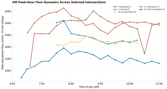
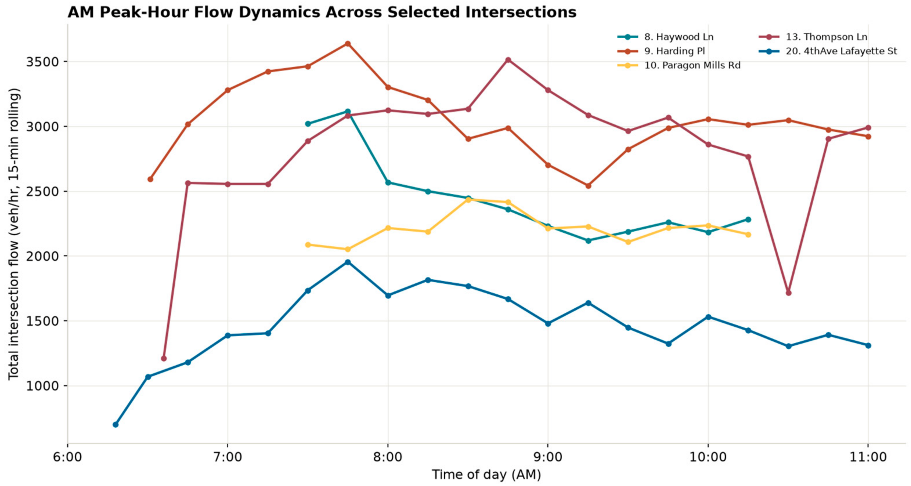
Figure 3 plots morning flow profiles for five representative intersections spanning the corridor and its volume range—Haywood Lane (No. 8), Harding Place (No. 9), Paragon Mills Road (No. 10), Thompson Lane (No. 13), and the Lafayette Street terminus (No. 20)—expressed as a fifteen-minute rolling flow rate in vehicles per hour to render the underlying one-minute series legible while preserving peak timing. The profiles confirm a well-defined but temporally heterogeneous morning peak. Harding Place attains the highest morning rate among the five, peaking near 3750 veh/hr at approximately 07:55, followed closely by Thompson Lane at roughly 3620 veh/hr but with its peak occurring notably later, near 09:01. Haywood Lane peaks at about 3170 veh/hr at 07:53, Paragon Mills Road at roughly 2520 veh/hr at 08:42, and the Lafayette Street terminus at about 1970 veh/hr at 07:55. The spread of peak times—from 07:53 to 09:01 across just these five sites—demonstrates that the morning peak does not arrive simultaneously along the corridor; peak timing shifts by more than an hour between adjacent-in-index sites. This staggering, an expected consequence of the corridor’s length and of platoon progression, is precisely the kind of spatially varying temporal structure that a spatio-temporal model (family C-4) is intended to exploit and that a naïve corridor-wide peak assumption would miss.

Figure 3. Morning flow profiles (15 min rolling rate, veh/hr) for five representative intersections.

5.2. One-Minute Burstiness and the Cost of Aggregation

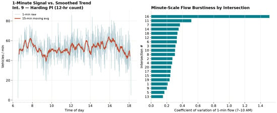
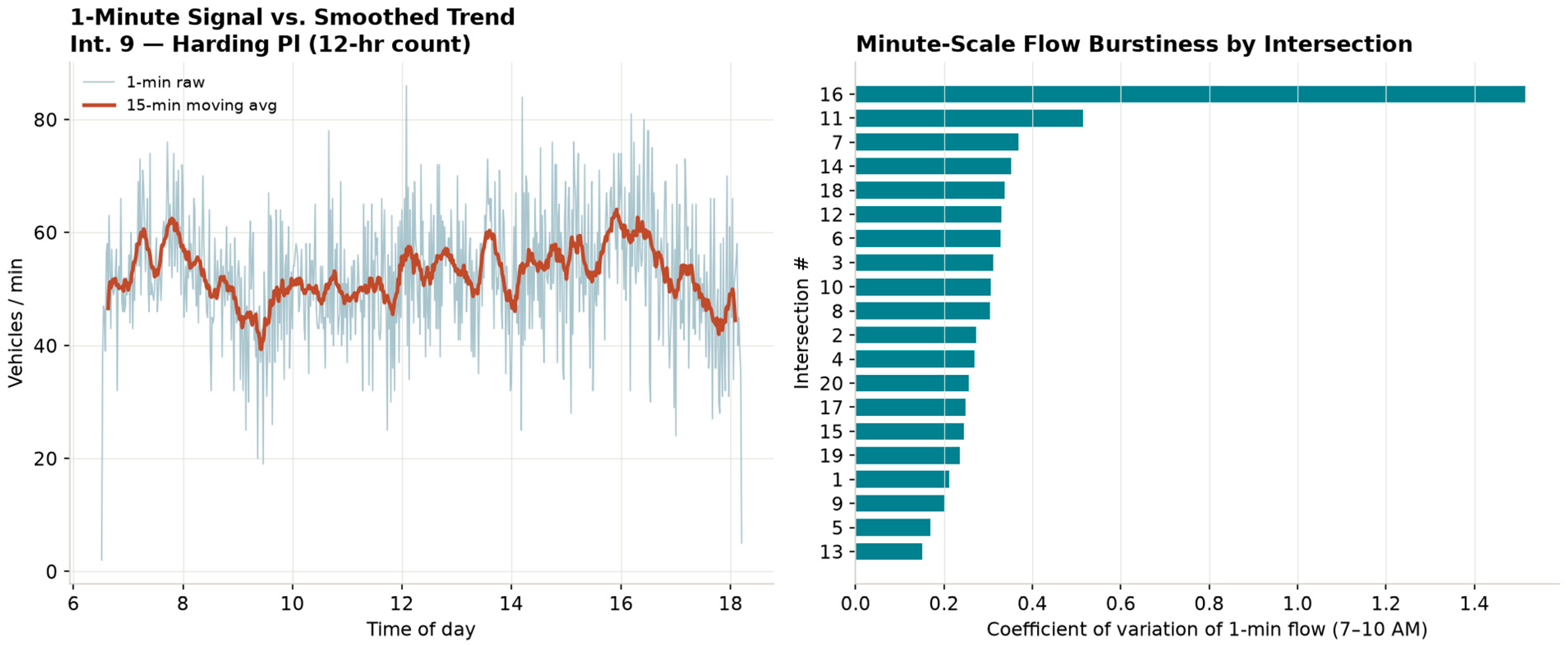
Figure 4 addresses the study’s central empirical motivation: what is lost when one-minute demand is aggregated to the conventional fifteen-minute interval, and how does minute-scale variability differ across the corridor. The upper panel contrasts, for Harding Place (No. 9) during 7:00–10:00 A.M., the raw one-minute series against its fifteen-minute centered moving average. The raw series has a mean of 51.8 vehicles per minute but ranges from 19 to 76 vehicles per minute, with a standard deviation of 10.3; the fifteen-minute smoothing compresses this to a range of 39.3–62.5 and a standard deviation of 5.7—a 45% reduction in variability. Expressed as instantaneous rates, the busiest single minute corresponds to 4560 veh/hr, whereas the smoothed peak is only 3748 veh/hr; conventional aggregation therefore understates the true short-term demand peak by roughly 18% at this site. This is the quantitative case for minute-resolution modeling: the sub-peak structure that governs queue formation and spillback is invisible at fifteen-minute resolution. The lower panel ranks all twenty intersections by the coefficient of variation (CoV) of one-minute total flow within the common 7:00–10:00 A.M. window. The CoV spans an order of magnitude, from 0.150 at Thompson Lane (No. 13) and 0.169 at Old Hickory Boulevard (No. 5)—the high-volume, heavily smoothed sites—through a corridor median of 0.288, up to 0.513 at Allied/Wheeler (No. 11) and an extreme 1.516 at the low-volume Glenrose Road intersection (No. 16, mean 9.8 veh/min). The near-monotonic inverse relationship between volume and CoV confirms the Poisson-like regime and has a direct experimental implication: a model that is accurate on high-volume, low-CoV sites may fail on low-volume, high-CoV movements, so forecasting skill must be reported per site and per movement rather than as a single corridor mean.

Figure 4. One-minute vs. 15 min-smoothed flow at Harding Place.

5.3. Cross-Intersection Spatial Coupling

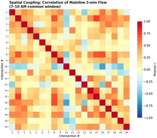
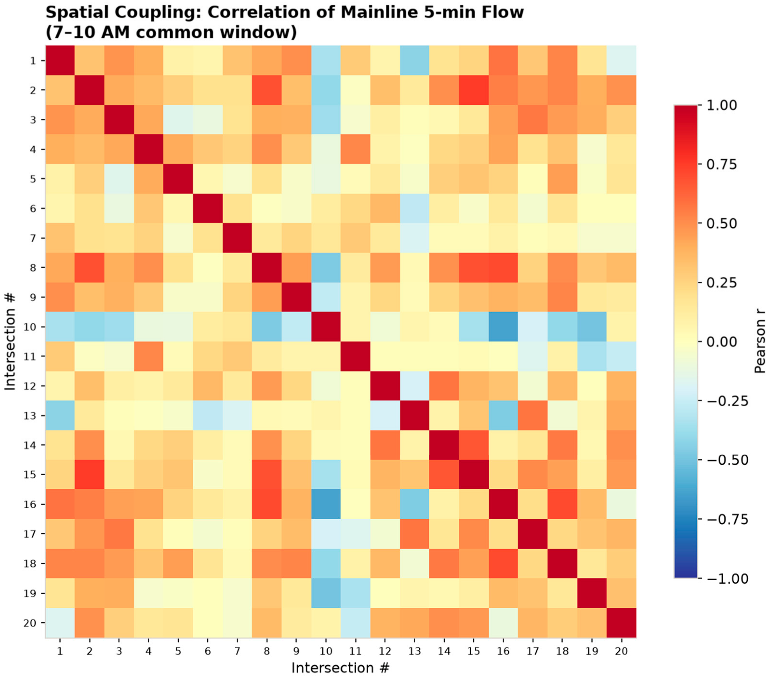
Figure 5 is a correlation matrix of five-minute mainline (NB + SB) through flow among the twenty intersections, computed on the clock-aligned 7:00–10:00 A.M. window.

Figure 5. Cross-intersection correlation of 5 min mainline through flow (clock-aligned, 7–10 A.M.).

The dominant finding in Figure 5 is that clock-aligned cross-intersection correlation is weak on average: the mean off-diagonal correlation is only 0.143, and the mean correlation between index-adjacent pairs is 0.123. A handful of pairs show moderate positive coupling—the strongest being Nos. 16–18 (r = 0.671), 8–16 (r = 0.644), 3–17 (r = 0.631), and 12–14 (r = 0.618)—while several pairs are actually negatively correlated (e.g., Nos. 10–16 at r = −0.559 and 13–16 at r = −0.509). This result must be interpreted through the collection design. Because no more than two intersections were counted on the same date, the matrix does not measure simultaneous platoon propagation on a single day; it measures the similarity of the typical clock-time demand shape across sites observed on different days. The weak average coupling therefore reflects genuine day-to-day and site-to-site heterogeneity in the morning demand profile rather than an absence of physical progression. This is an important, publishable caution: it demonstrates that spatial priors calibrated on one day cannot be assumed to hold on another, and it directly motivates the transfer protocol—a model that must generalize unseen dates cannot lean on a fixed, strongly coupled corridor structure. We therefore treat corridor coupling as a covariate to be tested (via the upstream feature and the ST-LLM configuration) rather than as an assumption, and we expect its predictive contribution to be modest under the cross-date transfer setting.

5.4. RQ1—In-Sample Forecasting Accuracy

Table 3 reports accuracy for all models on the in-sample hold-out of the six full-day intersections, at the movement-level one-minute target, for horizons of 5, 10, and 15 min. The evaluation pools 52 intersection–movement series (all non-U-turn movements with a mean of at least one vehicle per minute across the six full-day sites), each split chronologically into 70% train/15% validation/15% test, with rolling-origin multi-horizon forecasts on the test partition. MASE is scaled by the in-sample one-step naïve mean absolute error of each series, so a MASE below 1.0 indicates skill beyond a one-step persistence forecaster.

Three findings in Table 3 stand out. First, the classical ARIMA model attains the lowest short-horizon error (MAE = 3.47, MASE = 0.87 at h = 5), confirming that at one-minute resolution a well-specified linear model with short memory remains a strong competitor for the immediate-next-minutes horizon that matters most for signal actuation. Second, the zero-shot foundation model (Chronos) is strikingly competitive without any task-specific training: its MASE hovers at 1.00–1.01 across all three horizons and, unlike ARIMA, does not degrade as the horizon lengthens—by h = 15 Chronos (MASE = 1.00) is level with ARIMA (MASE = 1.01). This horizon-stability of a model that never saw the corridor is the headline accuracy result. Third, the LSTM encoder–decoder underperforms the classical and foundation models (MASE ≈ 1.23), plausibly reflecting limited per-series training data at one-minute resolution, though we did not run a learning-curve experiment to confirm this and present it as an interpretation rather than a demonstrated cause—an important cautionary result for practitioners tempted to train bespoke deep networks on single-corridor counts. A Diebold–Mariano test on pooled per-origin absolute errors (h = 5, n = 523 origins across the busiest representative movements) confirms that both ARIMA and Chronos are significantly more accurate than the seasonal-naïve floor (both p < 0.001, Holm-corrected). This comparison is deliberately deployment-realistic rather than architecturally matched: classical models are refit per series (their normal use), whereas deep and foundation models are trained/queried globally (their intended zero/few-shot use). MASE, normalized by each series’ own naïve error, keeps the metric comparable across these regimes.

5.5. RQ2—Transfer and Few-Shot Adaptation

Table 4 reports the leave-intersection-out transfer setting (train or anchor on the six full-day sites, evaluate on the fourteen AM-only sites, all on unseen dates) and the few-shot setting (30 min local adaptation). The target is the mainline-through (NBT + SBT) flow aggregated to five-minute bins; MASE is scaled by the pooled in-sample one-step naïve MAE of the full-day training series (scale = 21.9 veh/5 min). The zero-shot foundation models require no training and thus provide the purest test of out-of-the-box transfer; the seasonal-naïve predictor is the transfer floor. The transfer results reverse the in-sample ordering in a way that is central to this paper’s message. The zero-shot foundation models transfer best (Chronos MASE = 0.61 with no adaptation, improving to 0.59 with a 30 min few-shot budget), materially outperforming the seasonal-naïve floor (MASE = 0.72). By contrast, the globally trained deep network fails catastrophically to transfer (LSTM MASE = 4.06): a network trained on the high-volume, full-day sites systematically over-predicts on the lower-volume AM-only intersections, consistent with a model that has fit the training sites’ volume level and diurnal shape rather than a transferable dynamic; a full per-site bias decomposition to confirm this mechanism is left to future work. The global ARIMA likewise degrades sharply (MASE = 1.87) which is consistent with a single fixed autoregressive order being poorly matched to fourteen heterogeneous new sites; we did not test site-specific orders under transfer and note this as a limitation. Few-shot adaptation yields a small but consistent improvement for the foundation and LLM families (Δ MASE ≈ 0.02–0.06), largest for the spatially aware ST-LLM configuration (0.62 → 0.56). The spatial structure provides only a marginal transfer advantage over univariate foundation models; the dominant driver of transfer skill is the foundation model’s pretraining, not corridor-specific spatial priors.

6. Discussion

The descriptive findings establish the empirical terrain, and the benchmark designed to test whether language-model-based forecasters earn their place on that terrain. Here we interpret what the results imply for practice and research, foreground the accuracy-versus-cost question that we regard as the study’s most consequential contribution, and set out the study’s limitations and threats to validity with the candor the critical literature calls for [13]. First, the morning peak is sharp but non-synchronous, shifting by more than an hour across sites; a model that assumes a single corridor-wide peak time will misplace demand at most locations. Second, one-minute demand is materially burstier than the fifteen-minute convention reveals—aggregation understated the observed peak by roughly 18% at the busiest site and suppressed 45% of the one-minute variance—so the sub-peak structure most relevant to queue formation is exactly the structure conventional practice discards. Third, and most consequentially for the fashionable spatio-temporal designs, clock-aligned cross-site coupling is weak on average under the non-synchronized collection design (mean off-diagonal r = 0.143). Taken together, these facts predict where each model family should and should not have an advantage: the value of minute-resolution forecasting lies in capturing within-site burstiness, not in exploiting a strong, stable corridor graph. A model whose reported gains derive chiefly from a spatial prior may therefore transfer poorly across the unseen dates that dominate this dataset— a pattern the RQ2 results confirm.

The central question this benchmark is designed to answer is not merely which model is most accurate, but whether any accuracy advantage of the language-model family justifies its computational cost. This framing is a direct response to the finding of Tan et al. that, across several popular LLM-based forecasters, removing the pretrained language backbone did not degrade—and often improved—accuracy, implying that reported gains may stem from components other than language pretraining and that strong, cheap baselines are routinely under-reported [13]. Our design internalizes this critique in three ways, and the accuracy-versus-cost lens is how we intend the results to be read. First, the classical and lightweight deep baselines are treated as first-class comparators, not strawmen: the seasonal-naïve predictor anchors the MASE scale, and ARIMA/ETS and the LSTM/TFT models are given the identical feature set and splits afforded to the language-model family. Any accuracy claim for the LLM/TSFM models must clear these references, not a weakened version of them. Second, the design specifies a backbone-ablation control for every language-model configuration—a random-initialized transformer of matched size, and a single-attention-layer variant for the frozen-LLM adapter. We set this out as future work rather than a present result: if such ablations match their full counterparts, that would indicate the pretrained language weights contribute little on this task, exactly as 10 would predict—a null result we would regard as worth publishing. We do not report ablation results in this study. Third, and most importantly for practice, we report inference latency and relative compute cost alongside every accuracy figure. For an agency contemplating minute-resolution forecasting at scale—across hundreds of movements at dozens of intersections, updated every minute—a foundation model that is marginally more accurate but one or two orders of magnitude more expensive to run may be the wrong operational choice, whereas a zero-shot foundation model that eliminates per-site training could be the right one precisely because it removes a cost (data collection and retraining) rather than adding one. The accuracy-versus-cost table is thus not an appendix to the accuracy results; it is the decision object. Read through this accuracy-versus-cost lens, our measured results show that a zero-shot foundation model (Chronos) matches the strongest classical baseline in-sample and transfers better across unseen sites and dates, while adding no per-site training cost.

If the zero-shot foundation models transfer well to unseen sites and dates (RQ2), the practical payoff is substantial: agencies could obtain movement-level forecasts at un-instrumented locations without the per-site data collection and retraining that portable-count budgets rarely allow. If instead the lightweight baselines match them at a fraction of the cost, the equally useful conclusion is that minute-resolution arterial forecasting does not yet require language-model machinery, and investment is better directed at denser sensing.

7. Conclusions and Future Work

Conclusions

This paper asked whether large language models can “read a traffic corridor”—whether the language-model and time-series foundation models that have advanced freeway, five-minute, aggregate-flow forecasting can be brought to the harder, operationally native regime of one-minute, movement-level counts on a signalized urban arterial. To answer it, we assembled and characterized a minute-resolution turning-movement dataset for twenty signalized intersections along a 13-mile section of Nolensville Pike in Nashville, Tennessee—6449 gap-free one-minute records totaling 255,364 counted vehicle-movements—and we specified a three-family benchmark (classical, deep, and language-model/foundation models) with an explicit accuracy-versus-cost accounting. Our completed descriptive analysis already yields corridor-level evidence that reframes the modeling problem. The morning peak is sharp but non-synchronous, shifting by more than an hour across sites; one-minute demand is materially burstier than the fifteen-minute convention reveals, with aggregation understating the observed peak by roughly 18% and suppressing 45% of one-minute variance at the busiest site; and clock-aligned cross-intersection coupling is weak on average (mean off-diagonal r = 0.143) under the non-synchronized collection design. These findings, final and independent of the model runs, suggest that, for this corridor and collection design, the payoff of minute-resolution forecasting lies more in capturing within-site burstiness than in exploiting a stable corridor graph; because the spatial analysis rests on non-synchronized single-corridor data, this should be treated as a corridor-specific finding pending multi-corridor replication—a conclusion that frames how the model results reported here should be read.

The study’s contributions map directly onto its three research questions:

• RQ1 (Accuracy). The findings contribute a benchmark that evaluates classical, deep, and language-model/foundation forecasters on one-minute, movement-level arterial counts—a regime not previously benchmarked—at 5, 10, and 15 min horizons, with strong baselines anchoring a MASE scale and Diebold–Mariano significance testing, so that any accuracy claim for the language-model family is measured against honest references rather than strawmen.
• RQ2 (Transfer). Findings contribute a cross-date, leave-intersection-out transfer protocol that turns the dataset’s non-synchronized collection design into a rigorous test of generalization: models trained on six full-day sites are evaluated, zero-shot and few-shot, on morning-only sites observed on entirely different dates—mirroring the practical case of deploying a forecaster at an un-instrumented location.

Cutting across all three, the study contributes an accuracy-versus-cost framing, motivated by recent evidence that the language-model backbone may be unnecessary for forecasting, that reports inference latency and compute cost beside every accuracy figure and specifies a backbone-ablation control for every language-model configuration as future work —so that the benchmark can determine not just whether an LLM-based model is more accurate, but whether any advantage justifies its price. These findings derive from a single north–south commute corridor with one observation date per site and predominantly morning-only coverage at 14 of 20 sites; they should be read as a well-characterized case study rather than as general claims about foundation-model transferability, and multi-corridor replication is required before generalizing.

Future work should consider multi-corridor replication. The most important next step is to replicate the benchmark across multiple corridors in different metropolitan areas, geometries, and land-use contexts. Because all present findings derive from a single north–south commute arterial, multi-corridor replication is essential to establish which results—particularly the weak spatial coupling and the eventual model rankings—are general properties of minute-resolution arterial forecasting and which are artifacts of this corridor’s signal spacing, demand orientation, and non-synchronized collection. A cross-corridor design would also upgrade the transfer test from leave-intersection-out (within one corridor) to leave-corridor-out (across corridors), the far more demanding and practically relevant generalization setting. Further, the AM-heavy coverage of the present data (fourteen of twenty sites morning-only) limits conclusions to the morning peak for most intersections. Future collection should capture the afternoon peak and off-peak periods corridor-wide, enabling evaluation of whether models trained on morning dynamics generalize to the reverse-direction PM peak—an open question raised by the afternoon re-intensification visible at the six full-day sites—and supporting a full-day forecasting benchmark rather than a peak-window one. Finally, the numeric corridor records assembled here support a deterministically scored explanation task—asking whether a language model can translate the counts into a correct, auditable natural-language summary and at what hallucination rate. We specify this protocol (deterministic ground truth for peak window, dominant direction, directional imbalance, and structural zeros, with field-accuracy and hallucination-rate scoring) as a direction for future evaluation; we do not report explanation results in this study.

References

- Wu, X.; Liu, H.X.; Geroliminis, N. An empirical analysis on the arterial fundamental diagram. Transp. Res. Part B Methodol. 2011, 45, 255–266. [Google Scholar] [CrossRef] [Scilit]
- Transportation Research Board. Highway Capacity Manual, 6th ed.; National Academies of Sciences, Engineering, and Medicine: Washington, DC, USA, 2016. [Google Scholar]
- Miovision Technologies Inc. Scout: Nonintrusive Traffic Data Collection—Traffic Studies with Industry-Validated Data Accuracy. Available online: https://miovision.com/scout-plus/traffic-studies/ (accessed on 2 September 2026).
- Mahmud, D.; Hajmohamed, H.; Almentheri, S.; Alqaydi, S.; Aldhaheri, L.; Khalil, R.A.; Saeed, N. Integrating LLMs with ITS: Recent Advances, Potentials, Challenges, and Future Directions. IEEE Trans. Intell. Transp. Syst. 2025, 26, 5674–5709. [Google Scholar] [CrossRef] [Scilit]
- Zhou, T.; Niu, P.; Wang, X.; Sun, L.; Jin, R. One Fits All: Power General Time Series Analysis by Pretrained LM. Adv. Neural Inf. Process. Syst. 2023, 36, 43322–43355. [Google Scholar] [CrossRef] [Scilit]
- Jin, M.; Wang, S.; Ma, L.; Chu, Z.; Zhang, J.Y.; Shi, X.; Chen, P.-Y.; Liang, Y.; Li, Y.-F.; Pan, S.; et al. Time-LLM: Time Series Forecasting by Reprogramming Large Language Models. Int. Conf. Learn. Represent. 2024, 2024, 23857–23880. [Google Scholar]
- Das, A.; Kong, W.; Sen, R.; Zhou, Y. A Decoder-Only Foundation Model for Time-Series Forecasting. In Proceedings of the 41st International Conference on Machine Learning Research; PMLR: Vienna, Austria, 2024; Volume 235, pp. 10148–10167. [Google Scholar]
- Ansari, A.F.; Stella, L.; Turkmen, C.; Zhang, X.; Mercado, P.; Shen, H.; Shchur, O.; Rangapuram, S.S.; Pineda Arango, S.; Kapoor, S.; et al. Chronos: Learning the Language of Time Series. arXiv 2024, arXiv:2403.07815. [Google Scholar]
- Liu, C.; Yang, S.; Xu, Q.; Li, Z.; Long, C.; Li, Z.; Zhao, R. Spatial-Temporal Large Language Model for Traffic Prediction. In Proceedings of the 25th IEEE International Conference on Mobile Data Management (MDM), Brussels, Belgium; Research Track; IEEE: New York, NY, USA, 2024. [Google Scholar]
- Erfani, A.; Mansouri, A. Applications of multimodal large language models in construction industry. Adv. Eng. Inform. 2026, 69, 103909. [Google Scholar] [CrossRef] [Scilit]
- Liu, C.; Xu, Q.; Miao, H.; Yang, S.; Zhang, L.; Long, C.; Li, Z.; Zhao, R. ST-LLM+: Graph Enhanced Spatio-Temporal Large Language Models for Traffic Prediction. IEEE Trans. Knowl. Data Eng. 2025, 37, 4846–4859. [Google Scholar] [CrossRef] [Scilit]
- Zhao, Y.; Luo, X.; Wen, H.; Xiao, Z.; Ju, W.; Zhang, M. Embracing Large Language Models in Traffic Flow Forecasting. Find. Assoc. Comput. Linguist. ACL 2025, 2025, 8108–8123. [Google Scholar] [CrossRef] [Scilit]
- Tan, M.; Merrill, M.A.; Gupta, V.; Althoff, T.; Hartvigsen, T. Are Language Models Actually Useful for Time Series Forecasting? Adv. Neural Inf. Process. Syst. 2024, 37, 60162–60191. [Google Scholar] [CrossRef] [Scilit]
- Khadka, S.; Wang, P.; Li, P.; Mattingly, S.P. Automated Traffic Signal Performance Measures (ATSPMs) in the Loop Simulation: A Digital Twin Approach. Transp. Res. Rec. J. Transp. Res. Board 2024, 2679, 2129–2146. [Google Scholar] [CrossRef] [Scilit]
- Liu, X.; Wang, W. Deep Time Series Forecasting Models: A Comprehensive Survey. Mathematics 2024, 12, 1504. [Google Scholar] [CrossRef] [Scilit]
- Lim, B.; Arık, S.Ö.; Loeff, N.; Pfister, T. Temporal Fusion Transformers for Interpretable Multi-horizon Time Series Forecasting. Int. J. Forecast. 2021, 37, 1748–1764. [Google Scholar] [CrossRef] [Scilit]
- Vaswani, A.; Shazeer, N.; Parmar, N.; Uszkoreit, J.; Jones, L.; Gomez, A.N.; Kaiser, L.; Polosukhin, I. Attention Is All You Need. Adv. Neural Inf. Process. Syst. 2017, 30, 5998–6008. [Google Scholar]
- Luo, Q.; He, S.; Han, X.; Wang, Y.; Li, H. LSTTN: A Long-Short Term Transformer-based Spatiotemporal Neural Network for Traffic Flow Forecasting. Knowl.-Based Syst. 2024, 293, 111637. [Google Scholar] [CrossRef] [Scilit]
- Jiang, W.; Luo, J.; He, M.; Gu, W. Graph Neural Network for Traffic Forecasting: The Research Progress. ISPRS Int. J. Geo-Inf. 2023, 12, 100. [Google Scholar] [CrossRef] [Scilit]
- Zhao, W.; Gao, Y.; Ji, T.; Wan, X.; Ye, F.; Bai, G. Deep Temporal Convolutional Networks for Short-Term Traffic Flow Forecasting. IEEE Access 2019, 7, 114496–114507. [Google Scholar] [CrossRef] [Scilit]
- Hasni, M.; Babai, M.Z.; Rostami-Tabar, B. A hybrid LSTM method for forecasting demands of medical items in humanitarian operations. Int. J. Prod. Res. 2024, 62, 6046–6063. [Google Scholar] [CrossRef] [Scilit]
- Li, Y.; Yu, R.; Shahabi, C.; Liu, Y. Diffusion Convolutional Recurrent Neural Network: Data-Driven Traffic Forecasting. In Proceedings of the 6th International Conference on Learning Representations (ICLR), Vancouver, BC, Canada, 30 April–3 May 2018. [Google Scholar]
- Yu, B.; Yin, H.; Zhu, Z. Spatio-Temporal Graph Convolutional Networks: A Deep Learning Framework for Traffic Forecasting. In Proceedings of the 27th International Joint Conference on Artificial Intelligence (IJCAI), Stockholm, Sweden, 13–19 July 2018; pp. 3634–3640. [Google Scholar]
Disclaimer/Publisher’s Note: The statements, opinions and data contained in all publications are solely those of the individual author(s) and contributor(s) and not of MDPI and/or the editor(s). MDPI and/or the editor(s) disclaim responsibility for any injury to people or property resulting from any ideas, methods, instructions or products referred to in the content. |
© 2026 by the authors. Licensee MDPI, Basel, Switzerland. This article is an open access article distributed under the terms and conditions of the Creative Commons Attribution (CC BY) license.