


Abstract
In this paper we investigate the potential of Magnifying Networks, an architecture recently proposed in the domain of digital pathology, in the realm of satellite imagery analysis, an increasingly important remote sensing modality of practical significance in a wide range of domains. In particular, we address the challenges posed by the extreme size of satellite images and the inadequacy of the current state of the art in capturing salient information across scales while remaining computationally feasible. Specifically, we adapt the MagNet architecture by adjusting the number of magnifying layers and by employing the softmax function as a specific mechanistic means in the exploratory search within each magnifying layer. In addition, we conduct a series of comparative experiments to identify effective design choices and their effect on performance in the specific context of satellite remote sensing. Focusing on the most challenging classes in the Functional Map of the World with small object-to-image ratios, the adapted MagNet surpasses an Inception-v3 baseline (AUROC vs. , Accuracy vs. , F1-score vs. ), supporting adaptive magnification as an effective modelling approach to gigapixel satellite imagery.
1. Introduction
The introduction of satellite remote sensing in the late 20th century has allowed humanity to observe our planet on a previously unprecedented scale and efficiency; it has changed how we analyse our environments, manage agriculture and support fields such as urban planning, land use management, and infrastructure development [1,2,3,4].
Advances in sensor technology now enable satellite images to capture from vast geographical areas (e.g., a single Sentinel-2 tile captures on average a 110 km × 110 km area) to pixels representing an on-the-ground area of cm2, and hyperspectral capabilities, resulting in images with with close to billions of pixels (commonly referred to as gigapixel images) [5,6,7,8]. In addition to the inherent, semantic challenges in analysing satellite imagery, their aforementioned gigapixel scale presents a major difficulty by virtue of its computational impositions. In particular, conventional deep learning architectures, which have emerged as the leading approaches over the course of the last decade, struggle to process and learn from gigapixel images end-to-end [9]. This is primarily a consequence of the current hardware constraints [9,10]. Although, the latest generations of GPUs deliver enhanced speed and increased memory, the resolution of images and videos captured by modern devices continues to rise at a high pace [9].
A common solution is to partition images into smaller patches, e.g., using non-overlapping exhaustive tiling, process these patches individually, and then aggregate the patch-wise inferences into a single inference per image [11,12,13]. While this data preprocessing approach enables off-the-shelf deep learning solutions to be adopted, it results in geometric and relational information loss that would otherwise be useful to a model, and also may introduce artefacts at the patch boundaries [14]. Moreover, for supervised training of deep learning models, patch-based preprocessing necessitates adapting ground truth annotations to each patch, a process that is rarely trivial and often requires significant manual effort. Alternatives that go beyond exhaustive tiling or random sampling have emerged, formalizing patch selection into the optimization process [8,15].
Herein, we explore the potential of Magnifying Networks (MagNets), originally proposed for whole-slide histopathology images, for use on satellite imagery. MagNets process the entire input image first, but at a coarse, low resolution level (e.g., pixels), thereafter iteratively analysing a small set of subpatches (e.g., pixels each) where evidence is likely to reside. Patch selection is optimised end-to-end and is thereof learnt automatically, reaching the overall decision also in a learning fashion, learning saliency across magnification levels before committing to an image-level decision based on higher resolution subpatches (e.g., pixels) [8,16]. Prior work reported strong accuracy and AUROC while processing substantially fewer pixels than competing approaches on gigapixel slides [8]. Herein, we test whether the core coarse-to-fine zooming mechanism of MagNets transfers to satellite images and which design choices carry over.
In particular, our contributions are:
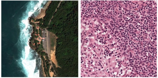
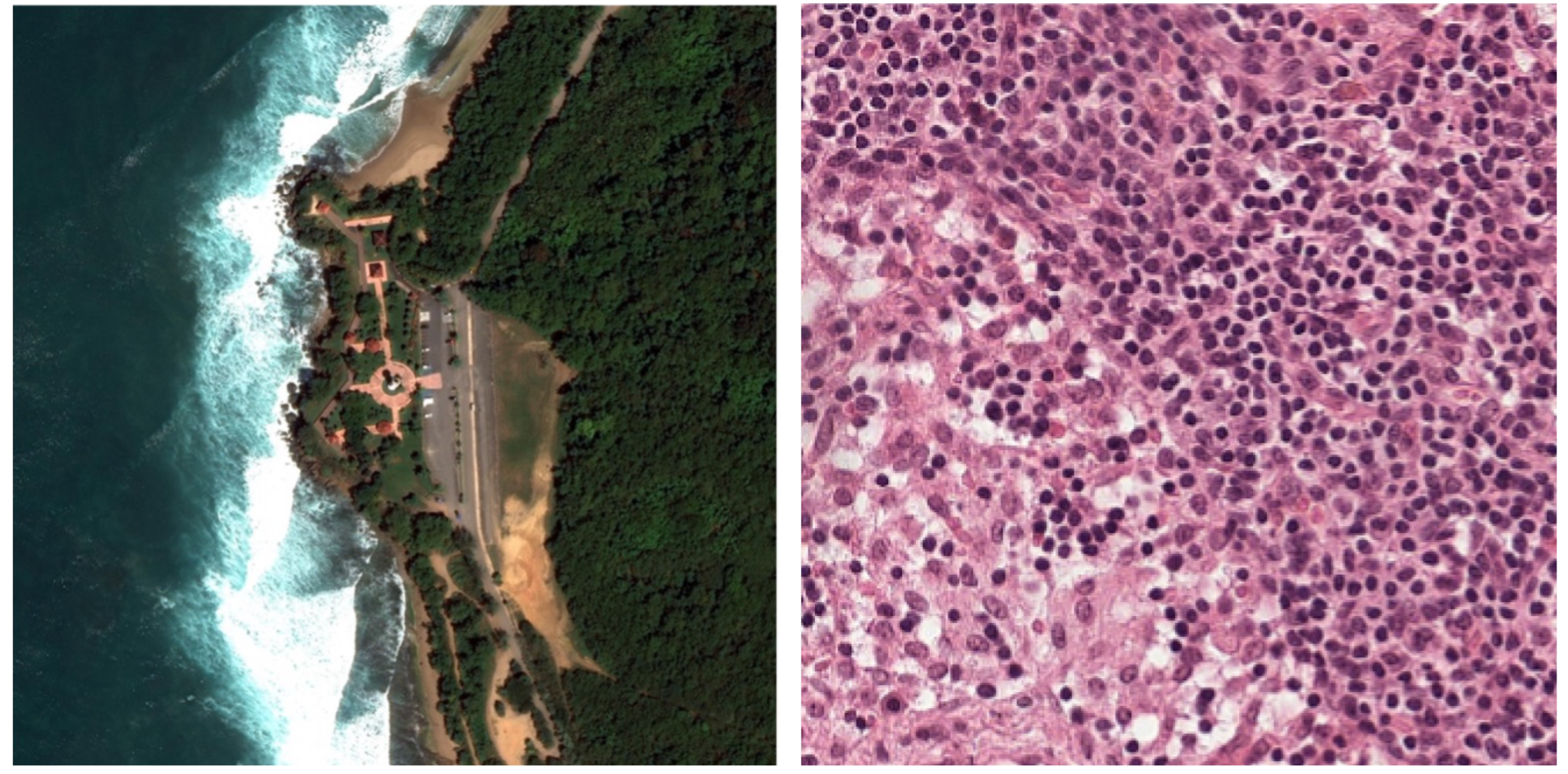
- We adapt MagNets to a new data domain (see Figure 1 for comparison) via architectural modifications, including reducing the number of magnifying layers from four to two and replacing sparsemax with softmax for exploratory search.
- We perform ablation studies to quantify the impact of these design choices on validation AUROC, F1-score, and accuracy.
- We demonstrate that on a two-class subset of Functional Map of the World with small object-to-image ratios, the adapted MagNet surpasses an Inception-v3 baseline (AUROC vs. , Accuracy vs. , F1-score vs. ), supporting the MagNets’ mechanism of adaptive magnification as an effective approach for analysing gigapixel satellite images.
Figure 1.
(Left) A high-resolution satellite image sampled from fMoW, showing a coastal landscape with ocean waves, sandy shoreline, vegetated areas, and built infrastructure including a lighthouse. (Right) A histopathology image of stained healthy tissue under the microscope, highlighting distinct cell populations and their spatial interactions.
2. Related Work
This section reviews literature related to deep learning methodologies designed for handling very large (up to gigapixel-scale) satellite images, beginning with an overview of key characteristics and challenges posed by satellite data itself. It subsequently explores various methods aimed at addressing the computational and contextual limitations of traditional convolutional neural network approaches, specifically discussing patch-based methods, weakly supervised learning strategies, adaptive multi-scale architectures, graph-based contextual modeling, and recent advancements involving vision transformers.
2.1. Satellite Data Characteristics
Satellite imagery acquisition can be characterised by the following four key dimensions:
- Spectral Dimension. Refers to the sensor’s ability to detect reflectance across various wavelengths. Narrower wavelength channels such as those of a hyperspectral sensor allow for the capture of more detailed reflectance signatures, enabling precise differentiation between materials.
- Spatial Dimension. Defines the level of ground detail that is captured per pixel (e.g., very-high spatial resolutions translate to each pixel representing an on-the-ground area of less than 1 m2), as well as across all pixels, i.e., how extensive the geographic coverage is, for example, Sentinel-2 tiles span approximately 110 km × 110 km.
- Radiometric Dimension. Describes the sensor’s sensitivity in detecting differences in brightness or radiance levels. Higher radiometric resolution translates into finer granularity of recorded brightness levels, enabling subtle variations in surface reflectance to be effectively distinguished.
- Temporal Dimension. Captures the frequency at which successive images are acquired for a specific area. Increased acquisition frequency enhances the detection and monitoring of dynamic phenomena, events and objects of interest.
This multi-dimensional nature makes satellite imagery an invaluable asset across diverse applications—from environmental assessments to surveillance of human activities and disaster response.
2.2. Exhaustive Tiling Approaches
A common approach for handling very large satellite images is to divide them into smaller patches, e.g., using non-overlapping exhaustive tiling, that can be processed by standard CNN architectures, then aggregate the patch-wise predictions into an image-level result [9]. This patch-based tiling strategy enables use of off-the-shelf models, but it suffers from loss of global context and potential artifacts at patch boundaries [17]. Important spatial relationships that span across patches may be missed, as features extracted from one patch are not shared with neighbouring patches. Moreover, inference becomes slower because the model must process many patches separately [9]. Despite these drawbacks, patch-wise CNN classification has been widely used in remote sensing scene analysis. For instance, Muhammad et al. [18] proposed a Patch-Based Discriminative Learning framework for scene classification, which explicitly explores spatial dependencies between image regions to improve upon basic patch voting strategies. Similarly, Liu et al. [12] employed overlapping patches to minimise artefacts and smooth transitions between patches. While this method reduces some artefacts, it cannot fully preserve global relational and geometric information, as overlaps cannot account for non-adjacent patches. In another approach, Audebert et al. [13] used morphological operations to eliminate small artefacts at patch boundaries during segmentation tasks. However, this technique risks inadvertently removing areas of interest and does not address the loss of geometric and relational data. Such methods acknowledge the patch context problem but still fundamentally rely on tile based static preprocessing.
2.3. Weakly Supervised Learning and Multiple-Instance Learning Approaches
When only image-level labels are available for large images, multiple-instance learning (MIL) provides a useful framework to bridge the gap between local regions and global labels. In recent years, MIL has often been combined with CNN feature extraction to effectively capture local semantic cues associated with a scene label [19]. In a MIL setting, an image is treated as a “bag” of many small region instances; the model is trained to predict the scene label from the bag, typically by aggregating instance-level features via pooling or attention mechanisms [8,19]. This weakly supervised strategy avoids the need to assign ground-truth labels to individual patches. For example, Wang et al. (2018) use max- and average-pooling to aggregate patch features for remote sensing scene classification (originally applied to medical images), though such simple pooling may not fully capture complex spatial information in scenes [20]. More advanced MIL models introduce attention-based aggregation that learns to weight the contributions of each patch to the final prediction. A recent method by Dai et al. (2022) proposed a deep MIL with residual dense attention (MIL-RDA), enabling the network to focus on discriminative regions among many instances [19]. Overall, MIL approaches improve upon naive patch aggregation by learning which parts of a large image are most relevant to the scene label, under the constraint of only image-level supervision.
2.4. Adaptive Region Selection
Instead of statically processing a fixed grid of patches, several methods adopt adaptive strategies to improve the efficiency of analyzing large images. These approaches typically perform a preliminary scan of the input image to identify candidate regions, which are then examined at higher resolution. For instance, in the context of remote sensing, Wang et al. (2018) proposed a recurrent attention convolutional network (ARCNet) capable of sequentially selecting and processing informative regions of interest [21]. More recently, MagNets have been introduced as a nested, attention-based framework that extends this principle [15]. In particular, A MagNet consists of one or more magnifying layers and one classification layer. Each magnifying layer, given an input image, selects patches to be extracted for the next magnifying layer. These patches may be sampled from a more refined version of the original image than the input image, resulting in recursively finer spatial detail (smaller objects identifiable, e.g., cars) revealed over magnifying layers. The exponentially increasing number of patches extracted at each magnifying layer (e.g., two patches outputted in the first magnifying layer, four in the second, and eight in the third) ultimately pass by the classification layer (sequentially using a combination of a GRU, CNN, and FC layers) at the last magnifying layer. Therefore MagNets can be optimised on a downstream classification task that will attempt to solve using this learnt, directed, and multi-level patch selection capability [8].
In medical imaging applications—particularly cancer diagnostics using whole-slide histopathology images—MagNets have demonstrated significant computational efficiency. For example, a 4-layer MagNet achieved accuracy of 81% and an AUROC of 84%, distinguishing cancerous tissues from healthy regions [8]. Additionally, MagNets were notably efficient, processing approximately five times fewer pixels than previous state-of-the-art methods [8].
2.5. Graph-Based Context Modelling
Another line of recent research seeks to preserve and exploit the spatial relationships between regions via graph neural networks. Instead of treating image patches independently, graph-based models represent patches (or superpixels/regions) as nodes in a graph, with edges encoding their adjacency or feature similarity. A graph convolution network (GCN) can then propagate information between these nodes, allowing the model to learn intrinsic contextual attributes of the scene that a regular CNN might miss. For example, Pan et al. (2021) developed a Deep Feature Aggregation GCN (DFAGCN) for high-resolution scene classification [22]. They first extract multi-scale CNN feature maps from the image, then build a graph where each node corresponds to a patch in the feature map; the GCN is applied to reveal patch-to-patch correlations and refine the features before classification [22]. Similarly, other works have proposed dynamic graph learning that updates the graph structure based on the image content, or high-order graph convolution for capturing not just pairwise but higher-level region interactions [23,24]. These methods do not rely on a rigid patch grid processed by independent CNN passes; instead, they integrate regional information in a holistic graph, which can be seen as a departure from conventional patch-based pipelines.
2.6. Vision Transformers for High-Resolution Images
Lastly, inspired by advances in computer vision, researchers have begun exploring vision transformer architectures for extremely large remote sensing images. Transformers are memory demanding for large inputs, but newer designs use hierarchical or sparse attention to scale to bigger images. For instance, the Hierarchical Image Pyramid Transformer (HIPT) and LongViT models, initially developed for pathology, demonstrate that transformers can process gigapixel images by breaking them into tokens at multiple resolutions and learning representations in a coarse-to-fine manner [25]. Such transformer-based frameworks build a global understanding through self-attention across the image, and have shown promising results in capturing long-range dependencies [25]. In remote sensing, some early works apply transformers with local-window attention or Swin Transformer variants to large aerial images, aiming to capture both fine details and broad context. While these approaches are still emerging, they represent a modern direction for high-resolution image analysis beyond CNNs. In summary, whether through adaptive region-of-interest detection networks, graph models, or transformers, the trend in recent literature is toward end-to-end learning on gigapixel-scale data without exhaustive and static tiling. The present work adds to this corpus of work. In particular, given that adaptive and hierarchical learning have already been shown as effective in certain contexts, our aim herein is to provide preliminary evidence concerning the specific mechanism of learning-based directiveness of MagNets in the analysis of satellite images. Our experiments are focused on the kinds of classes/structures that prove most challenging to single-scale models.
3. Materials and Methods
3.1. Data Preparation
3.1.1. Original Data Set
The data set used in this work is derived from the Functional Map of the World (fMoW) corpus [26], a publicly available resource containing over 1 million satellite images from more than 200 countries. Each image in fMoW is annotated with bounding boxes indicating the functional purpose of various structures and land-use categories. The original data set includes temporal sequences (i.e., satellite images of the same location at different acquisition dates), multispectral imagery, and extensive metadata. In this work, we use the pan-sharpened RGB subset of fMoW. Image sizes range from to pixels, with a mean of million and a median of million pixels per image. The distribution is heavy-tailed: of images are ≥1 million pixels, are ≥10 million pixels, and are ≥100 million pixels.
3.1.2. Data Selection
Our data selection procedure comprised two distinct parts. In the first the fMoW dataset was filtered to include the eight classes with the highest average image-size-to-bounding-box ratio (see Table 1) The purpose here was twofold. One, we were looking to identify classes that are most challenging to standard, single-scale models. Two, to achieve this, we focused our attention on particularly small, and thus difficult to localize, structures. Thus, images were filtered based on minimum pixel width threshold (1520 pixels), and maximum cloud coverage () to ensure visibility of the regions of interest. We stress that our aim here was not to engineer an all-round best performing, practical system, but specifically to assess whether the learnt, directed, and multi-level attention-driven nature of MagNets provides benefit in the analysis of satellite images in particularly challenging cases; this is why excessive cloud coverage was avoided. For interpretative clarity and to avoid ambiguity errors, images with multiple boundary boxes from more than 1 class label were excluded. Baseline experiments using an InceptionNet-v3 classifier were performed on this eight-class subset (detailed in Appendix A) and per-class performance analysed. Two classes, fountains and swimming pools, proved to be particularly difficult to distinguish one from another. Providing some evidence in favour of our hypothesis, visual inspection suggested that, in the case of these classes, the object of interest often occupied a small fraction of the image, limiting the discriminative power of the baseline at the reduced resolution ( pixels in our case) required for standard CNN processing. Appendix A presents further detail of this baseline experiment.
Table 1.
Baseline experiment summary.
Given that MagNets incorporate magnifying layers designed to progressively zoom in on learnt salient regions, we hypothesised that these classes would benefit most from MagNet’s adaptive focus. This hypothesis drove the design of our next, main experiment (see Table 2). This experiment focused on a balanced binary task constructed around the two aforementioned classes. This design was purposeful, aimed at providing clear evidence concerning the value of MagNets’ adaptive magnification specifically. Thus, training of both InceptionNet-v3 and MagNet was performed under identical conditions, thereby eliminating pervasive confounds and facilitating a direct assessment of performance gains, if any, from focused magnification-based processing.
Table 2.
Main experiment summary.
3.1.3. Data Processing
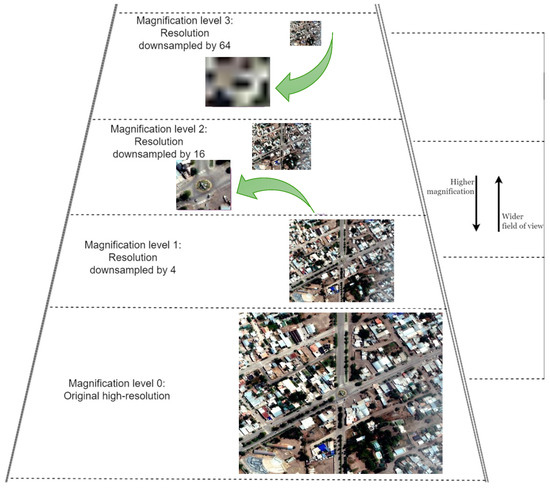
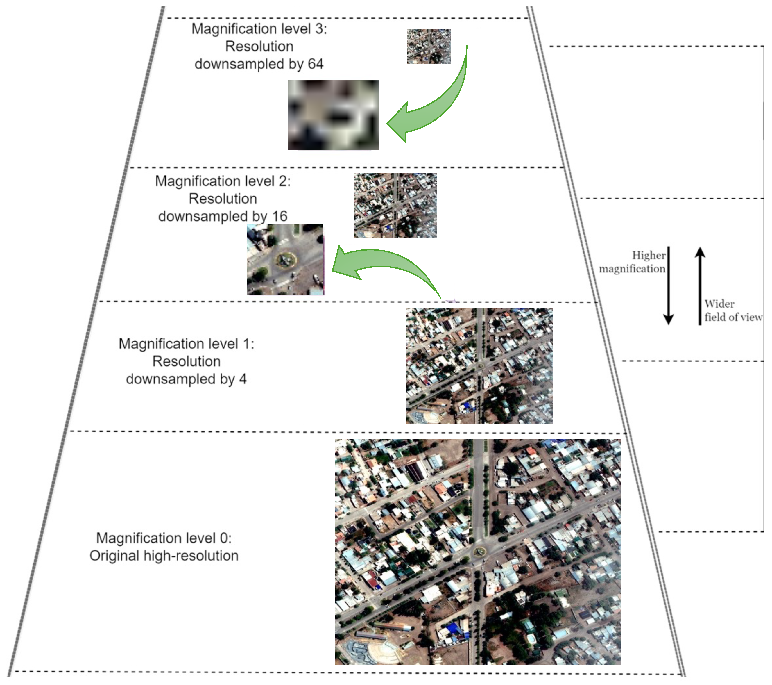
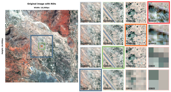
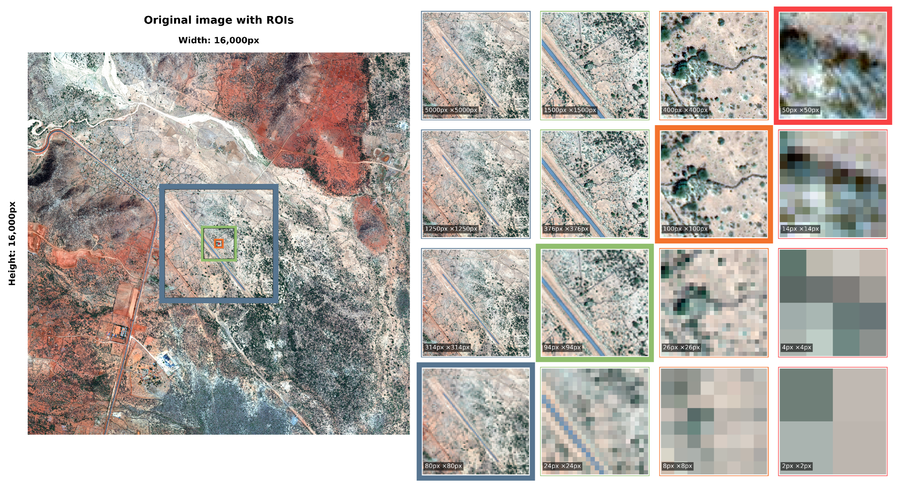
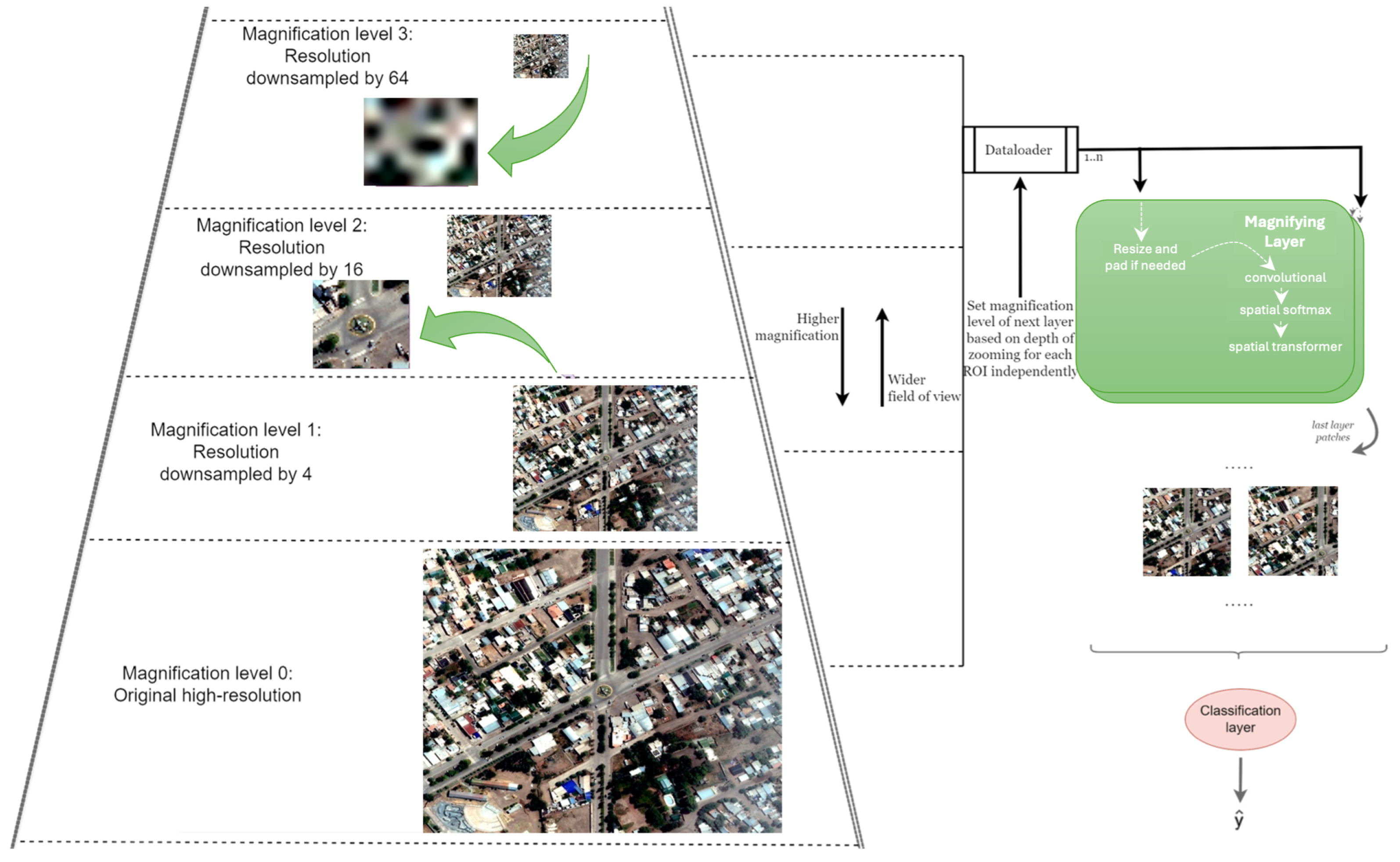
To prepare the images for training and inference using MagNets, we converted them into pyramidal TIFF format, creating four magnification levels, as shown in Figure 2. An image example following this convention is listed in Table 3—the original high-resolution image was designated as magnification level 0, with each subsequent level downsampled by a factor of four. This preprocessing enabled MagNets to dynamically load the appropriate magnification level corresponding to the current zoom-in scale of a requested ROI, avoiding the computational overhead of loading a very large portion of the image that would later get downsized; this is demonstrated in Figure 3.
Figure 2.
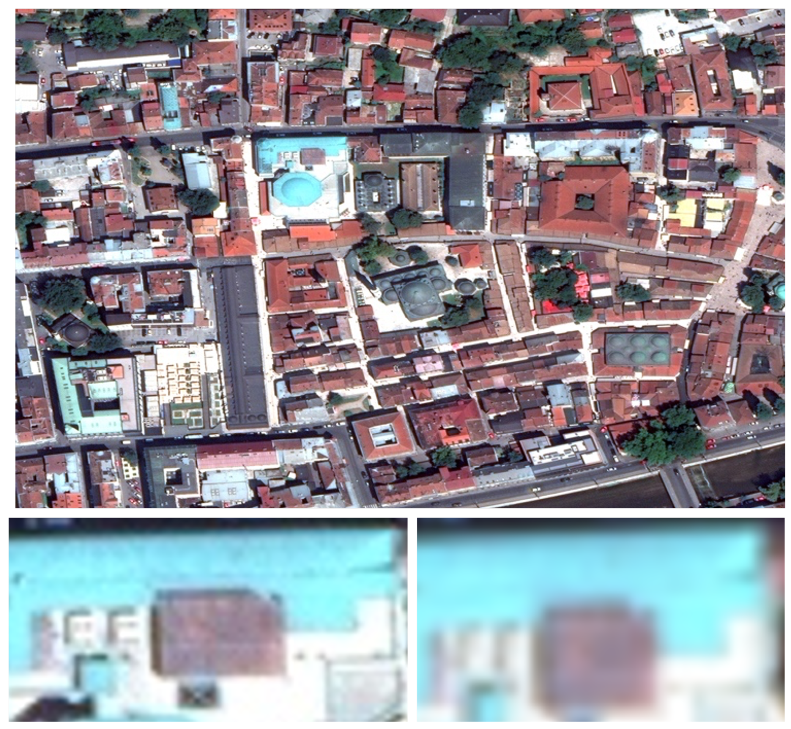
Pyramidal TIFF satellite image used in this study. Level 0 contains the original image with the highest resolution (minimum width 1520 pixels), while Level 3 represents the lowest resolution version (downsampled by a factor of 64). Green arrows indicate an example region retrieved from two different magnification levels.
Table 3.
Mapping a requested ROI (measured in Level-0 Width × Height pixels) to the appropriate pyramid level for a image example. Four magnification levels are available (L = 0 full resolution; L = 3 coarsest), with the Image size column listing the full-image dimensions at each level.
Figure 3.
Size-aware ROI retrieval with pyramidal TIFFs for MagNets. Left: the original image with four ROI requests (red: , orange: , green: , blue: —sizes given in level-0 pixels). For each ROI, the rows show the crop that would be returned from pyramid levels from top-to-bottom ( full resolution; coarsest). The highlighted panel marks the selected level, i.e., the coarsest level that still preserves sufficient detail for subsequent analysis, thereby avoiding over-fetching.
3.2. Magnifying Networks
3.2.1. Overview
MagNets perform adaptive, content-driven zooming. Beginning from a coarse (downsampled) view X ( pixels), each magnifying layer l uses convolutional features to drive a spatial transformer (STN) that parameterises a p number of affine crops . The key to learning-how-to-magnify is that each affine crop is applied to a larger, potentially higher spatial-resolution version of X, say ( pixels), where each pixel may correspond to a smaller on-the-ground distance. When the selected region is sufficiently small, the crop is extracted from a finer level of the image pyramid, allowing it to capture finer spatial detail than is represented in X. In this way, the network learns to magnify recursively, in a coarse-to-fine manner through end-to-end optimization of a downstream task, i.e., without needing ground truth for the boundary boxes. At the last magnifying layer, all tiles are sampled to pixels and passed through an ImageNet-pretrained Inception-v3; a GRU aggregates the per-patch embeddings into an image-level representation that the classifier (fully-connected layers) maps to logits.
The key hyperparameters of MagNets include the number of magnifying layers, the number of zoom-ins at each magnifying layer (called patches in the original work), the auxiliary loss functions, the freezing of a specific patch in a specific magnifying layer (i.e., the affine parameters are pre-set and not learnt), and the optimization parameters. Herein, we also investigate the spatial transformer, which lies at the core of each magnifying layer, and specifically the low-level design choice to use sparsemax in the original work as opposed to a combination of softmax and sparsemax outputs, as well as the design choice in the original work to have a lower bound threshold of for s in STNs. This lower bound was originally introduced to prevent overly aggressive zooming, which can lead to training instability and degraded extracted patch quality. In particular, since patches are extracted from an already sampled image (), selecting an excessively small region to zoom-in on may yield a subpatch containing fewer pixels than the expected input size of the next layer. At extreme values of s (e.g., ) this resulted in blurry and poorly resolved image patches. In subsequent magnifying layers, however, finer spatial detail can be recovered, as the new is extracted from a dynamically selected image representation with sufficiently fine spatial resolution to minimise excessive downsampling or upsampling for the next layer. For further information, we direct the reader to the work of Dimitriou et al. [8].
3.2.2. Magnifying Layers
Responding to the smaller image sizes in the Functional Map of the World dataset (average 8.2 MB, compared to the 50 GB typical of the Camelyon dataset used in the original paper), in this work we reduced the number of magnifying layers. The original work reported experiments with two, three, and four magnifying layers and observed gains on whole-slide images of pixels [8]. Given that images from fMoW are one to two orders of magnitude smaller (see Section 3.1.1), here we performed experiments with two and three magnifying layers. Our two versus three magnifying layer comparison showed no measurable improvement in performance, which, considering the compute costs involved, supports the use of two magnifying layers (see Appendix B).
3.2.3. Zoom-Ins per Magnifying Layer
At each magnifying layer, MagNets extract a configurable number of regions of interest (ROIs), or “patches”. Increasing the number of patches broadens the exploration but increases computation exponentially with depth [8]. For example, a three-layer MagNet with 2 patches selected at each magnifying layer will have 1, 2, and 4 images processes in the magnifying layers of pixel dimensions, and 8 patches of size processed by the classification layer.
3.2.4. Spatial Transformer Network
Each magnifying layer contains a spatial transformer network (STN) that parameterises a differentiable hard-attention crop operation. Following the original MagNet formulation, the STN comprises a localization network, grid generator, and sampler [8]. The localization network operates on a feature map (extracted using convolutional layers given a pixel image input) and produces an isotropic scale s and translations that define an affine transformation :
As in the original work [8], we constrain the parameters to stabilize early training and avoid degenerate crops:
Note that is set to in the original work but we experimented with varying its value in the ablation study. The probability map used to infer is produced by a spatial activation applied channel-wise to the last convolutional feature map. Herein, we experiment with a weighted combination of softmax and sparsemax over the lattice.
3.2.5. “Frozen” Patch
To preserve a global field-of-view when the first magnifying layer zooms aggressively, we follow the original design [8] and include a frozen patch at the second magnifying layer. Concretely, at magnifying layer 2 one patch is initialised to cover the entire layer-input (, ) and its localization parameters are held fixed throughout training. This guarantees that, irrespective of prior zoom-ins, one stream always propagates coarse contextual evidence into the classifier.
3.2.6. Auxiliary Losses
The reduction to two magnifying layers implied that further modifications were needed with respect to the auxiliary loss functions. Three and four-layer MagNets compute auxiliary losses using patch extracted at the first and the third magnifying layers. Instead, we use the patches from the second rather than the third magnifying layer. (shown in Figure 4). These outputs are then used in the same way as before: the paradoxical loss enforces that predictions from the deeper layer (layer 2) should not underperform those from the earlier layer (layer 1), while the cross-entropy loss continues to provide weak supervision by aligning the auxiliary predictions with the ground-truth image-level labels [8]. In this way, the auxiliary classifiers retain their intended roles despite the architectural adjustment to two magnifying layers.
Figure 4.
Overview of the modified MagNet architecture used in this study. The model takes a pyramidal TIFF image as input and performs adaptive, content-driven zooming through successive magnification levels. Each magnifying layer combines convolutional layers, spatial softmax, and a spatial transformer to focus on informative regions, which are then processed by a ResNet-18 for classification. Diagram adapted from Dimitriou et al. [8].
4. Evaluation
4.1. Evaluation Metrics
Model performance was evaluated using AUROC, accuracy, and F1-score. Accuracy can be defined as follows:
where , , , and denote the counts of true positives, true negatives, false positives, and false negatives, respectively. F1-score is defined as the harmonic mean of precision and recall:
where Precision represents the ratio of true positive predictions to the total number of positive predictions made, and Recall is the ratio of true positive predictions to the total number of actual positives. The Area Under the ROC Curve (AUROC) is defined as the integral of the true positive rate as a function of the false positive rate.
4.2. Data Set Splits
In order to ensure that accuracy, F1-score, and inter-class confusion metrics are not distorted by class imbalance, we sought to create a balanced binary data set comprising the two classes of interest, namely fountains and swimming pools. To this end, we sampled an equal number of images from each , yielding 252 images in total (126 per class). Stratification was applied in the subsequent data set splitting, maintaining class balance across the different subsets. The final partition comprised 168 training images, 42 validation images, and 42 test images, corresponding to the 66.7/16.7/16.7 split.
4.3. Data Augmentation
To improve generalisation, data augmentation was applied during training. The transformations included random horizontal and vertical flips, rotations of 90°, 180°, and 270°, and random colour jitter to adjust brightness and saturation by up to and of the original values, respectively. These augmentations emulate the range of viewing angles, lighting conditions, and seasonal variations present in satellite imagery, encouraging the network to learn features robust to such variability.
4.4. Ablations and Model Selection
All ablations were run three times with different random seeds; we report mean and standard deviation across seeds. We employed early stopping based on validation AUROC with a patience of 15 epochs.
4.4.1. Hyperparameter Tuning
We conducted a grid search over optimisers (Adam [27], NAdam [28], AdamW [29], RMSprop [30], and SGD [31]), batch sizes {4, 8}, and learning rates , , . AdamW with a learning rate of and batch size 8 yielded the most stable convergence, and we adopted these settings in subsequent ablations.
4.4.2. Patch Configuration
To evaluate the effect varying the number of patches selected and extracted at each magnifying layer of a two-layer MagNet, we conducted experiments with configurations , , and . As shown in Table 4, the configuration consistently achieved the highest AUROC. Constraining the second magnifying layer to attending to a single patch proved highly detrimental to performance, whereas increasing the number of patches in the first magnifying layer from two to three did not yield further improvements over the setup.
Table 4.
Patch-configuration ablation for the two-layer MagNet.
4.4.3. Attention Mechanism and Scale Bound
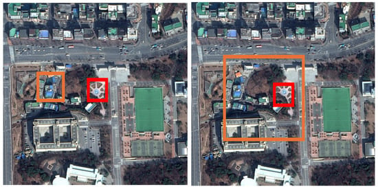
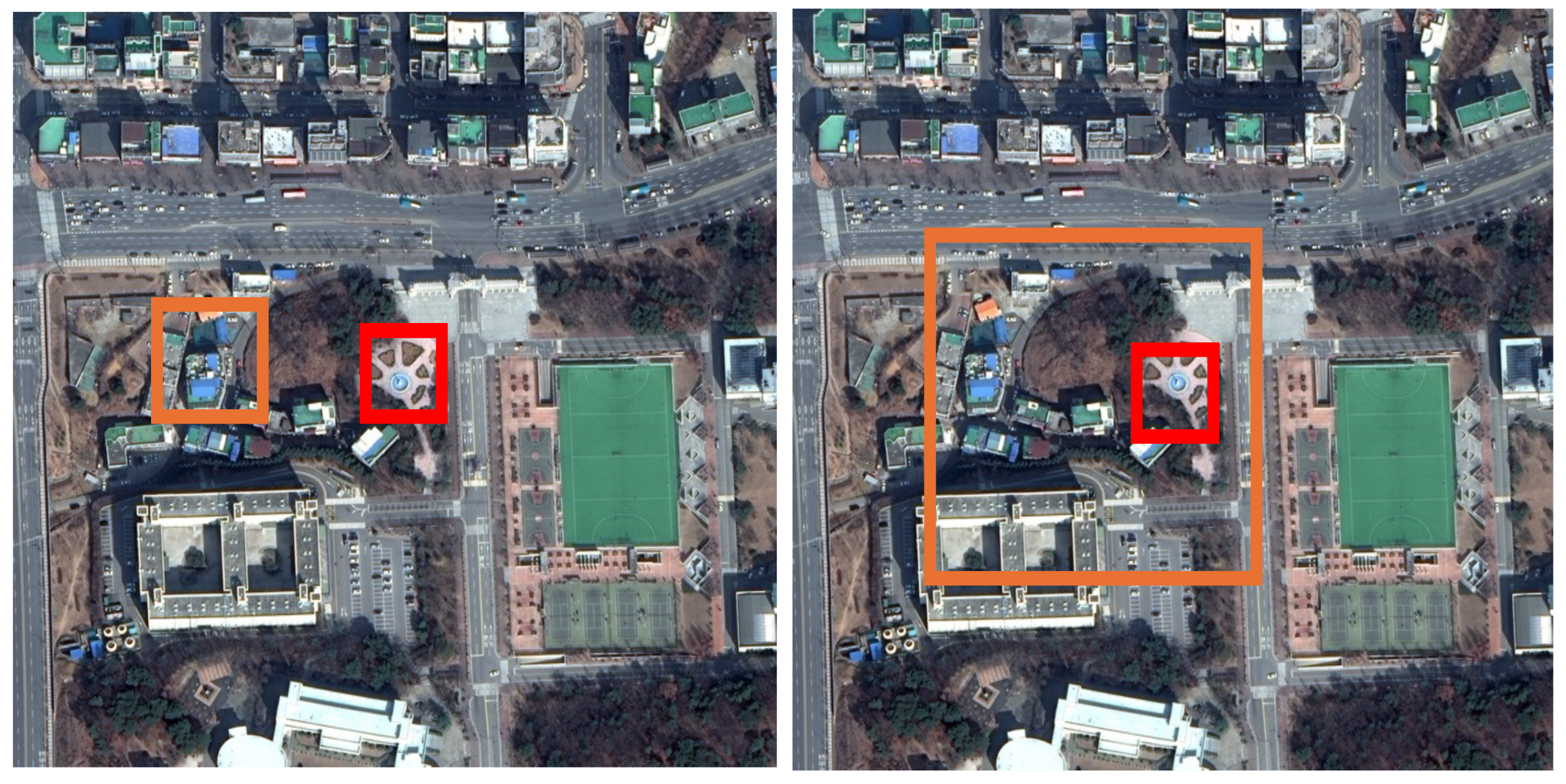
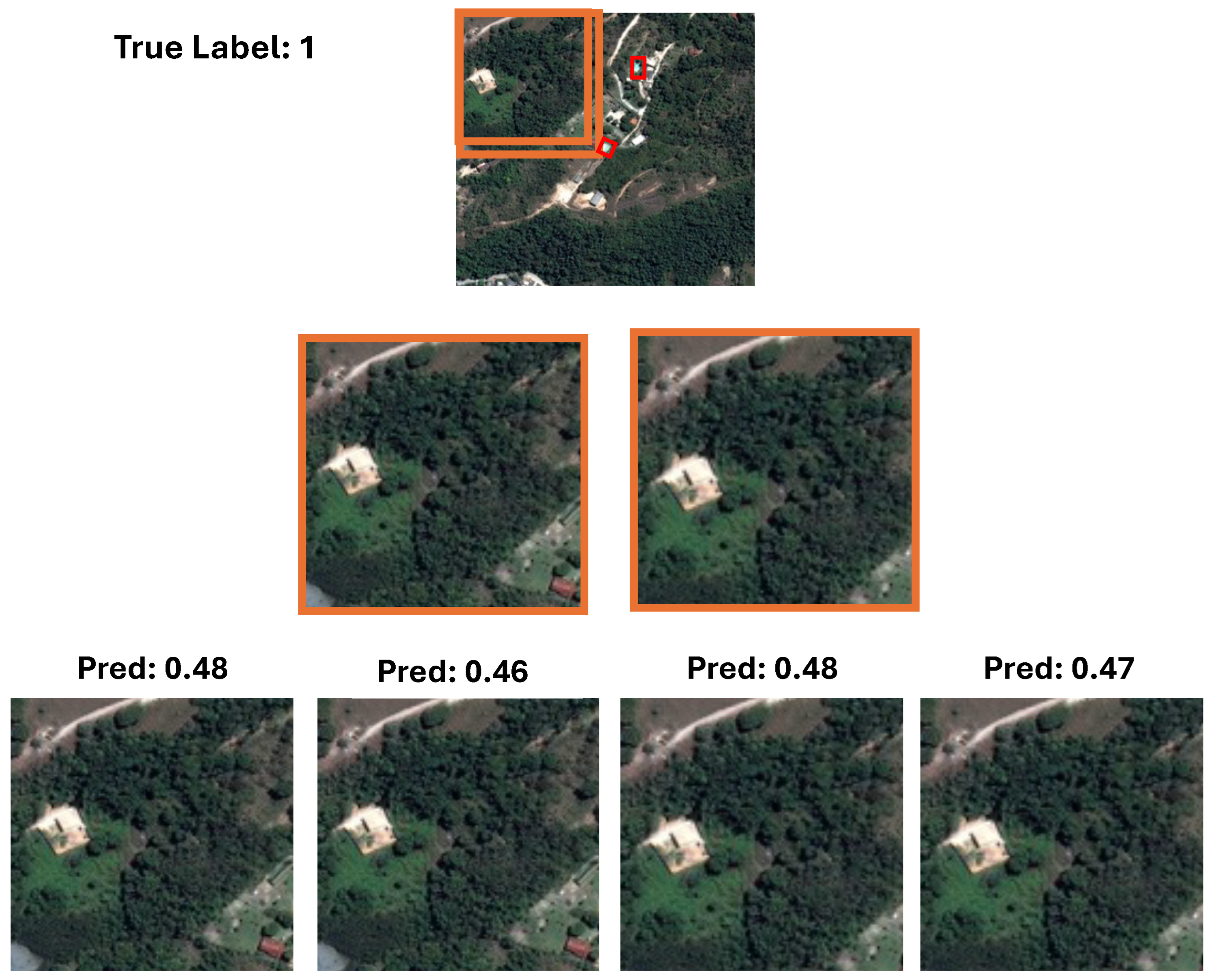
We next investigated the activation function within the spatial transformer networks (STNs). Three variants were compared: sparsemax, softmax, and an equal mixture of the two. AUROC improved when softmax was used exclusively (Table 5), likely because it distributes attention more broadly, which is advantageous for heterogeneous satellite scenes. In contrast, sparsemax generated overly selective crops that sometimes excluded informative context (illustrated in Figure 5).
Table 5.
Results comparing the use of sparsemax, softmax, or a combination (governed by the coefficient) as the activation function within the spatial transformer network of each magnifying layer of a two-layer MagNet.
Figure 5.
Visualisation of the impact of changing the coefficient in the first layer of the network: from sparsemax (left, coef = 0) to softmax (right, coef = 1). Attention patches are depicted in orange, and bounding boxes are shown in red.
We also varied the minimum scale parameter of the STN. The results (Table 6) showed little sensitivity to this bound, in contrast to whole-slide histopathology, where MagNets were originally applied. In cancer detection, extreme zooming to the cellular level is indispensable to confirm malignancy, and thus increasing the lower bound on scaling substantially affects (negatively) performance. By comparison, satellite imagery does not require such aggressive magnification—objects of interest are larger and more visually distinct, and overly small values risk discarding important information. Notably, at the extreme (i.e., each patch crop spans at least half of the layer input in width and height), we observed substantially higher run-to-run variance in AUROC. Accordingly, we retain the originally set bound () in the final model.
Table 6.
Scaling-factor ablation for the two-layer MagNet.
4.4.4. Freezing the First Patch of the Second Layer
We examined the impact of freezing the first patch in the second magnifying layer, a mechanism designed to preserve global context [15] (see Section 3.2.5). While the mean AUROC remained unchanged between the frozen and unfrozen variants (Table 7), the unfrozen setting exhibited slightly higher variance across runs. Although the effect size was small, we opted to retain the original design choice of keeping the first patch of the second magnifying layer frozen.
Table 7.
Effect of freezing the first patch in the second magnifying layer.
4.5. Model Training
4.5.1. InceptionNet-v3 Model
For comparison, we trained an ImageNet-pretrained InceptionNet-v3 as a strong convolutional baseline on the same binary task (fountain vs. swimming pool). The rationale is twofold: (i) InceptionNet-v3 constitutes the patch-level backbone within our MagNet classifier head, so its standalone performance provides an informative lower bound; and (ii) by holding the classifier constant across models, improvements can be primarily attributed to the magnifying layers rather than to differences in the discriminative head.
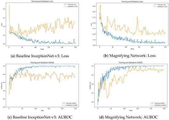
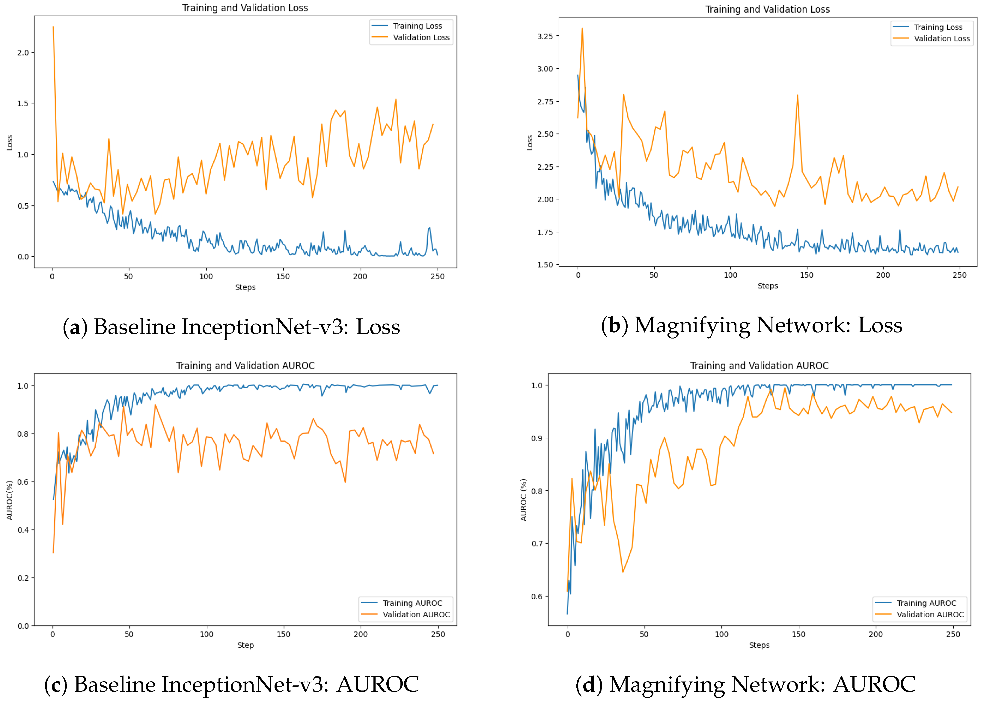
Inputs were resized to pixels. We first performed the grid search described in Section 4.4.1 and then trained the final baseline with the selected hyperparameters: AdamW optimizer, learning rate , and batch size 4. We trained for 250 epochs with the data augmentation described in Section 4.3, and monitoring loss and AUROC throughout training; the learning curves are shown in Figure 6a,c. This baseline establishes the capacity of a standard CNN to operate at a single, fixed scale without the coarse-to-fine exploration characteristic of MagNets.
Figure 6.
Learning curves of baseline InceptionNet-v3 and Two-layer Magnifying Network models.
4.5.2. Two-Layer Magnifying Network
Guided by the ablation study (Section 4.4), we trained a two-layer MagNet for the same task. The design choices follow the empirical findings: (i) two patches per magnifying layer (Section 4.4.2), (ii) spatial activations using softmax (coefficient ) in the localization network and a lower bound on the isotropic crop scale (Section 4.4.3), and (iii) the first patch in the second magnifying layer frozen (Section 4.4.4).
We trained for 250 epochs with the same augmentation protocol and tracked loss and AUROC over time; learning curves are shown in Figure 6b,d. Relative to the baseline, the MagNet thus differs only in its content-driven zoom-and-crop mechanism and auxiliary control of context flow, allowing us to ascribe downstream performance differences to the adaptive magnification itself.
4.6. Computational Cost Analysis
Computational efficiency is one of the main features of the MagNet architecture design that recommends MagNet use for very large images in particular. Here we concretise the benefits in the context of the data set adopted in the present paper.
The first point we make is that raw clock time, RAM and VRAM usage, and similar empirical metrics depend strongly on factors that are extrinsic to the examined method itself. Such factors include the particular hardware used, the software environment, the degree of code optimization, memory management strategy employed, batch scheduling, and data loading overhead. Measurements of this kind are undoubtedly useful when the method’s use in a specific, fixed deployment context is considered, but exhibit limited generalizability to different contexts. In other words, crude empirical analysis obscures the inherent and invariant methodological essence of the models compared. For this reason, here we pursue a different approach, comparing instead the characteristics of the behaviour that is intrinsic to the methods themselves. In particular, we report the numbers of pixels processed by different methods, namely the baseline and MagNets with different architectural variables; see Table 8.
Table 8.
Inference-time comparison of pixel counts examined by different models. For MagNets, the magnifying layers process pixels from each input image, and its classification layer processes images with pixels. For Inception-v3 models, the input patch size is given in the brackets. All patch sizes have three channels, but the channel dimension is omitted from the table for brevity.
As the baseline for our comparison, we used Inception-v3 having as input the whole-scene image at a resolution equal to the finest scale patch processed by MagNet (i.e., original image size). Since image size varies across the selected data, we report the two edge cases: the smallest image in the main experiment and the largest image in the fMoW dataset. This is the appropriate control for the present comparison because our goal is to provide evidence for the value of adaptive magnification of the MagNet’s key mechanism, which demands that the degree of local visual detail is kept constant.
4.7. Results and Discussion
Following our baseline experiment with eight classes, here we narrow our attention to the two that were found to be the most challenging ones, namely “fountain” and “swimming pool”. This focus allows us to draw conclusions about whether the specific region-selective and multi-scale approach of MagNets is effective precisely in the cases of classes that prove most difficult for single-scale models.
4.7.1. InceptionNet-v3 Results
The InceptionNet-v3 classifier performed moderately well in distinguishing between fountains and swimming pools, achieving an AUROC of 85%, F1-score of 76%, and accuracy of 71%. Notwithstanding its good performance according to all three metrics, we observed that the model exhibited some noteworthy classification challenges. In particular, the model relatively frequently misclassified images of fountains as swimming pools, with 10 out of 21 fountain images incorrectly identified, as shown in Table 9.
Table 9.
Performance statistics of the baseline InceptionNet-v3 binary classifier.
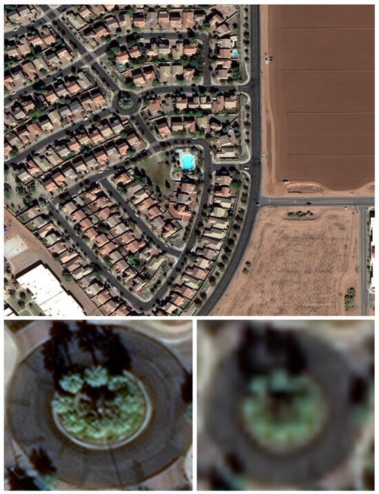
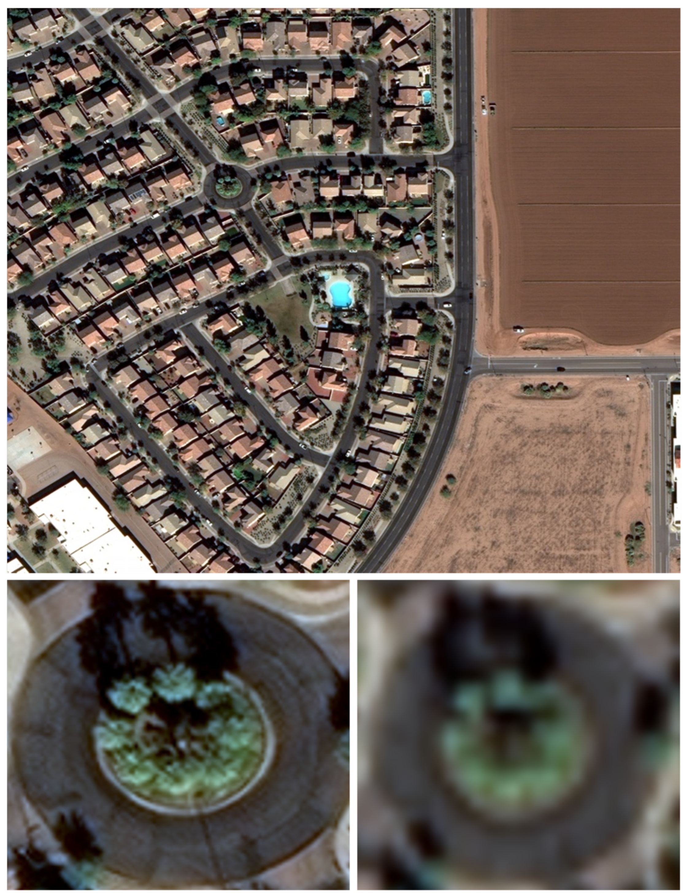
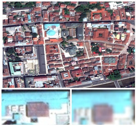
A visual examination of the misclassified images within the swimming pool class revealed that 3 out of 10 of these images included roundabouts (all three examples are shown in Appendix C Figure A3). Our qualitative assessment suggests that this confusion emanates from informational scarcity when the relevant structures are particularly small in scale (see Figure 7); this, however, remains a hypothesis at present and future empirical work should aim to establish a stronger evidential basis for the judgement.
Figure 7.
Image from the swimming pool class that was misclassified by InceptionNet-v3 and contained a roundabout.
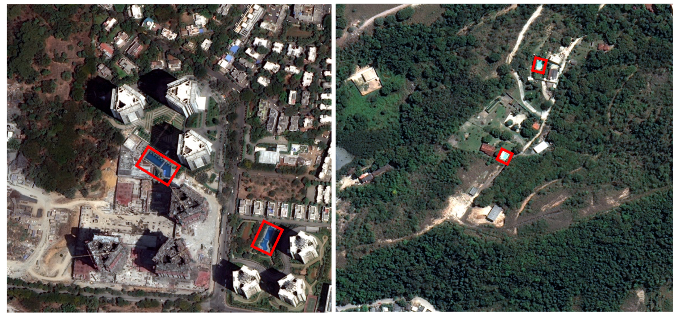
For the remaining 7 out of 10 misclassified images in the swimming pool class, visualised in Appendix C Figure A4, a common issue was identified. The regions of interest, specifically the swimming pools themselves, were significantly smaller in these misclassified images compared to those that were correctly classified. This observation is illustrated in Figure 8, which highlights the size discrepancy. This pattern suggests that swimming pools with smaller regions of interest may not be adequately visible to the network when the images are viewed at low resolutions.
Figure 8.
Comparison of bounding boxes (in red) of the swimming pool class between a correctly classified image by InceptionNet-v3 and an incorrectly classified image.
Additionally, the network misclassified 2 out of 21 fountain cases, as per Table 9. Upon closer examination of the images of fountains that were misclassified, it was observed that they both contained large rectangular blue objects, such as rooftops (both images are shown in Appendix C Figure A5). It seems that in a low-resolution setting, the InceptionNet-v3 model mistakes these blue objects as swimming pools.
4.7.2. Two-Layer MagNet Results
The final performance evaluation of the Magnifying Network demonstrated significant improvements over the baseline model, showcasing robust enhancements across several metrics. Specifically, the Magnifying Network achieved an AUROC of 89%, F1-score of 84%, and accuracy of 83%. These results highlight the network’s enhanced capability in handling the dataset compared to the initial baseline setup.
Most notably, there was a reduction of incorrect predictions for the swimming pool class, a category that had presented challenges for the baseline model, as shown in Table 10.
Table 10.
Performance statistics of the Magnifying Network binary classifier.
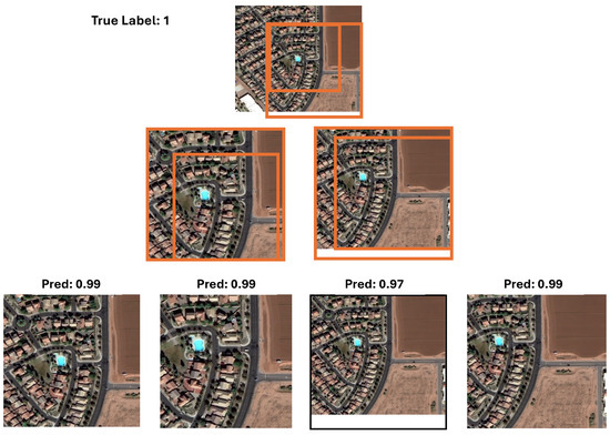
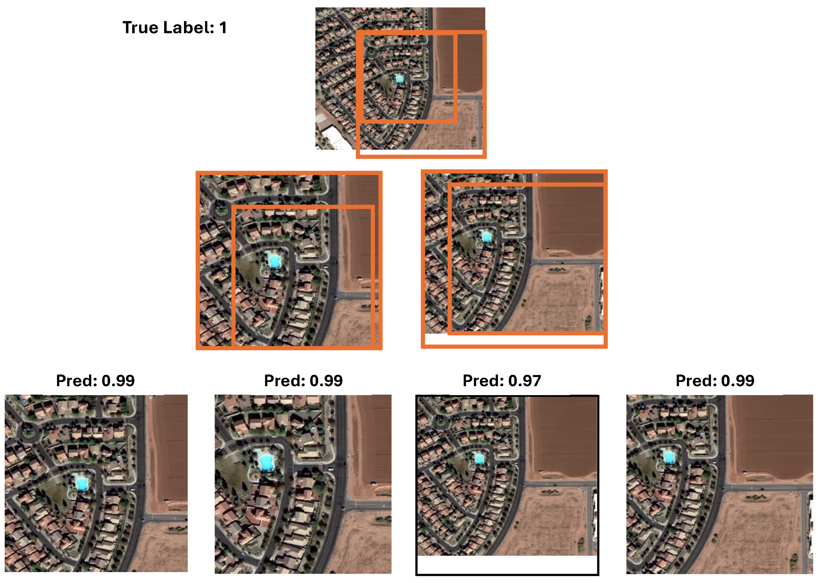
This suggests that the Magnifying Network’s ability to crop, zoom in, and view images at a higher resolution (through the magnifying layers) played a crucial role in discerning more details, particularly in distinguishing between a roundabout and a fountain, which allowed for more accurate classifications. One such example in shown in Figure 9.
Figure 9.
Illustration of Magnifying Network classifying an image in the swimming pool class containing a roundabout. Orange boundary boxes are the regions selected by each magnifying layer.
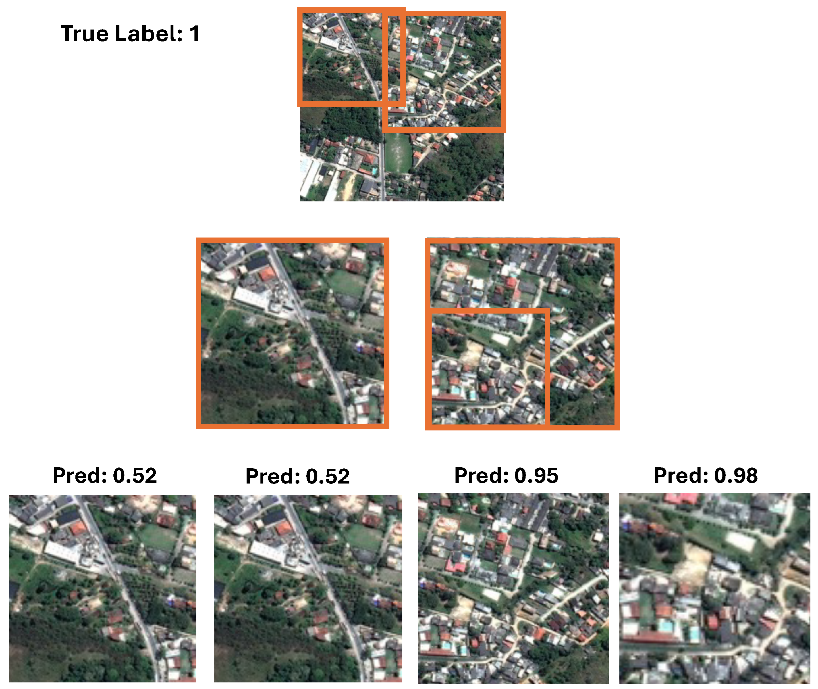
Moreover, this ability to zoom enhanced its effectiveness in detecting swimming pools with small regions of interest. One such example is shown in Figure 10. However, the network still faced challenges with swimming pools that had small, non-dispersed regions of interest, as depicted in Appendix C Figure A6 and Figure 11. This issue likely stemmed from the network not examining the image exhaustively; if it did not identify the swimming pool in the initial layer, it might have excluded it from the area of interest in subsequent layers, as illustrated in Figure 12.
Figure 10.
Illustration of Magnifying Network classifying an image in the swimming pool class with small, dispersed regions of interest. Orange boundary boxes are the regions selected by each magnifying layer.
Figure 11.
Image from the fountain class that was misclassified by InceptionNet-v3 as a swimming pool due to the presence of a large blue rectangular object.
Figure 12.
Illustration of Magnifying Network classifying an image in the swimming pool class with small, non-dispersed regions of interest. Bounding boxes of swimming pools are depicted in red. Orange boundary boxes are the regions selected by each magnifying layer. The ground truth is depicted as red boundary boxes.
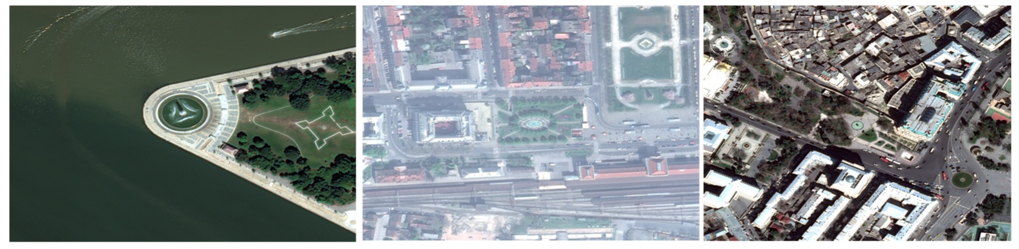
However, despite the overall enhancements, the Magnifying Network did not demonstrate a marked improvement over the baseline in accurately classifying fountains with 3 misclassifications made over the 2 of the baseline. All three cases are included in the appendix (Appendix C Figure A7).
5. Conclusions
In this paper we examined whether the recently proposed Magnifying Network architecture, featuring an efficient course-to-fine selection mechanism, can be adapted to satellite image classification when the structures of interest are small in comparison to the full image. Using a specific proof-of-concept target—guided by the availability of annotated data and the aim of presenting the algorithm with challengingly similar-looking structures—of distinguishing between fountains and swimming pools, we provided empirical evidence in favour of our hypothesis. We found that the adapted two-layer MagNet improved over a strong single-scale Inception-v3 baseline in AUROC, accuracy, and F1-score, with the benefit being most prominent for the class most affected by severe downsampling.
Our main contribution is a proof-of-concept, showing that MagNets and their mechanism of learnt, adaptive magnification remain useful outside of their original application domain of pathology. The work also illuminates which aspects of the model need greatest care when cross-domain adaptation is attempted; in the present case specifically, we demonstrated that a shallower architecture and softer localisation activation were beneficial alterations. Analytic, rather than empirical, compute comparison also suggests that a fixed number of classifier crops maintains performance well, comparing favourably with exhaustive high-resolution tiling which has to handle an exponentially growing number of pixels.
Several continuations building upon the contributions of the present paper present themselves. First, considering that our experiments focused on testing the value of the specific architectural feature of MagNets, namely their adaptive coarse-to-fine magnification mechanism, a natural next step for future work is to widen the range of baseline models. Such broader evaluation would provide additional evidence about how well the observations reported here generalize. In particular, it would be valuable to compare the present approach directly against stronger convolutional, transformer-based, and MIL-style baselines trained on the same task under identical conditions. Second, future work could explore leveraging stronger supervision while optimizing MagNets, e.g., by leveraging spatial information from boundary boxes to guide the magnifying layers or by providing patch-level class labels, when only image-level labels are available. As an example of such application in the satellite domain is change detection where the general area is known but not the specific locations that were impacted by a change.
Author Contributions
Conceptualization, E.H., O.A. and N.D.; methodology, E.H., O.A. and N.D.; software, E.H., N.D.; investigation, E.H.; writing—original draft preparation, E.H. and O.A.; writing—review and editing, E.H., O.A. and N.D.; visualization, E.H.; supervision, O.A. and N.D.; project administration, O.A. All authors have read and agreed to the published version of the manuscript.
Funding
N.D. was supported through the EU H2020 Research and Innovation Programmes under Grant Agreement No. 857586 (CMMI-MaRITeC-X) and No. 101158669 (AXOLOTL). Views and opinions expressed are however those of the author only and do not necessarily reflect those of the funding authorities.
Data Availability Statement
Data are available in a publicly accessible repository. The data presented in this work are openly available in multiple repositories, as listed here (accessed on 25 October 2024): https://github.com/fMoW/dataset [26].
Conflicts of Interest
The authors declare no conflicts of interest.
Abbreviations
The following abbreviations are used in this manuscript:
| Adam | Adaptive Moment Estimation |
| AdamW | Adaptive Moment Estimation with Weight Decay |
| AUROC | Area Under the Receiver Operating Characteristic curve |
| CNN | Convolutional Neural Network |
| NAdam | Nesterov-accelerated Adaptive Moment Estimation |
| ResNet | Residual Network |
| RMSprop | Root Mean Square Propagation |
| ROI | Region of Interest |
| SGD | Stochastic Gradient Descent |
Appendix A. Multiclass Classification
Initially, an ImageNet-pretrained InceptionNet-v3 was trained for scene classification of 8 classes using the SGD optimiser, a learning rate of , batch size of 4, and online data augmentation (see Section 4.3). The learning curve is shown in Appendix A Figure A1. The hyperparameters were tuned using the methodology described in Section 4.4.1.
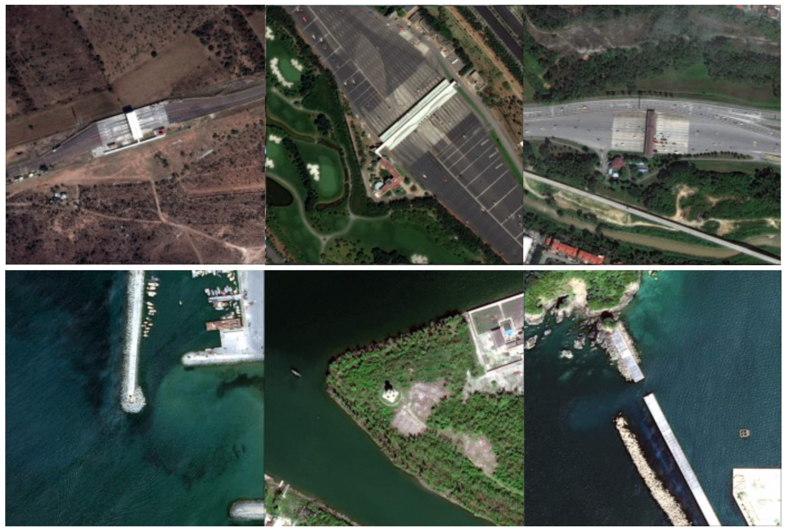
The classifier performed well in distinguishing classes with unique and easily identifiable contextual features. Notably, as shown in Table A1, it correctly identified 23 out of 25 toll booths and 21 out of 25 lighthouses. These classes benefit from their distinctive settings—toll booths are generally located near major roads, and lighthouses are typically found along coastlines, as highlighted in Figure A2.
However, the classifier encountered significant challenges when tasked with distinguishing between classes with similar contextual features, such as swimming pools and fountains, which are both typically located in residential areas. Misclassifications were notable: 6 out of 25 images of fountains were incorrectly identified as swimming pools, and 3 out of 25 swimming pool images were mislabelled as fountains.
Table A1.
Confusion matrix of the baseline InceptionNet-v3 multiclass classifier.
Figure A1.
Learning curves of baseline InceptionNet-v3 multi-class classifier.
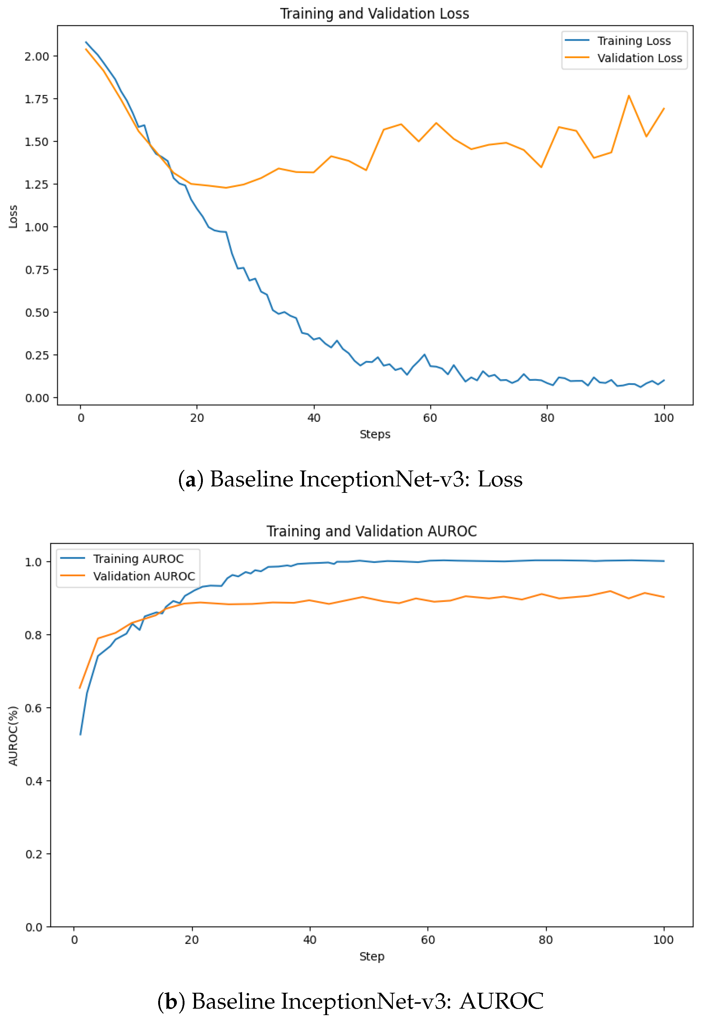
Figure A2.
Images from toll booth (top) and lighthouse classes (bottom).
Appendix B. Ablation on # of Magnifying Layers
The number of magnifying layers was the first architectural decision that had to be investigated with MagNets. Training was done on MagNets with hyperparameter configurations based on the original work [8]. Preliminary results showed no significant difference between the two- and three-layer models (see Table A2), so we adopted the shallower two-layer MagNet configuration.
Table A2.
Comparison of two- and three-layer MagNets using the original hyperparameter values.
Appendix C. Qualitative Results
Figure A3.
Misclassified images from swimming pool containing roundabouts by the InceptionNet-v3 baseline model.
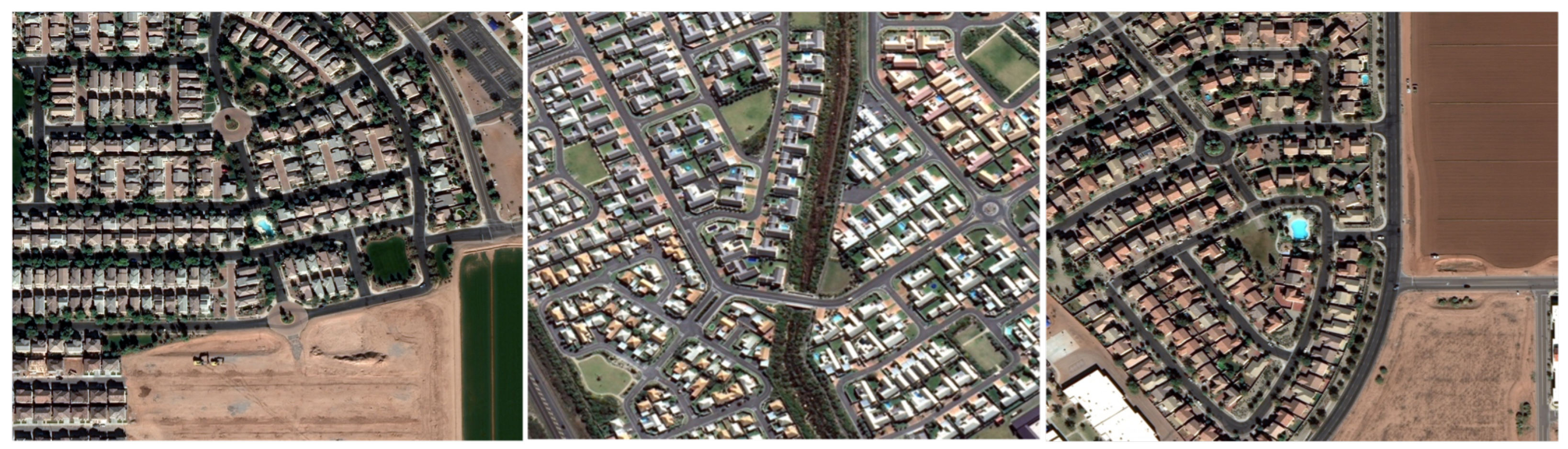
Figure A4.
Images from swimming pool class with small region of interest misclassified by the InceptionNet-v3 baseline model.
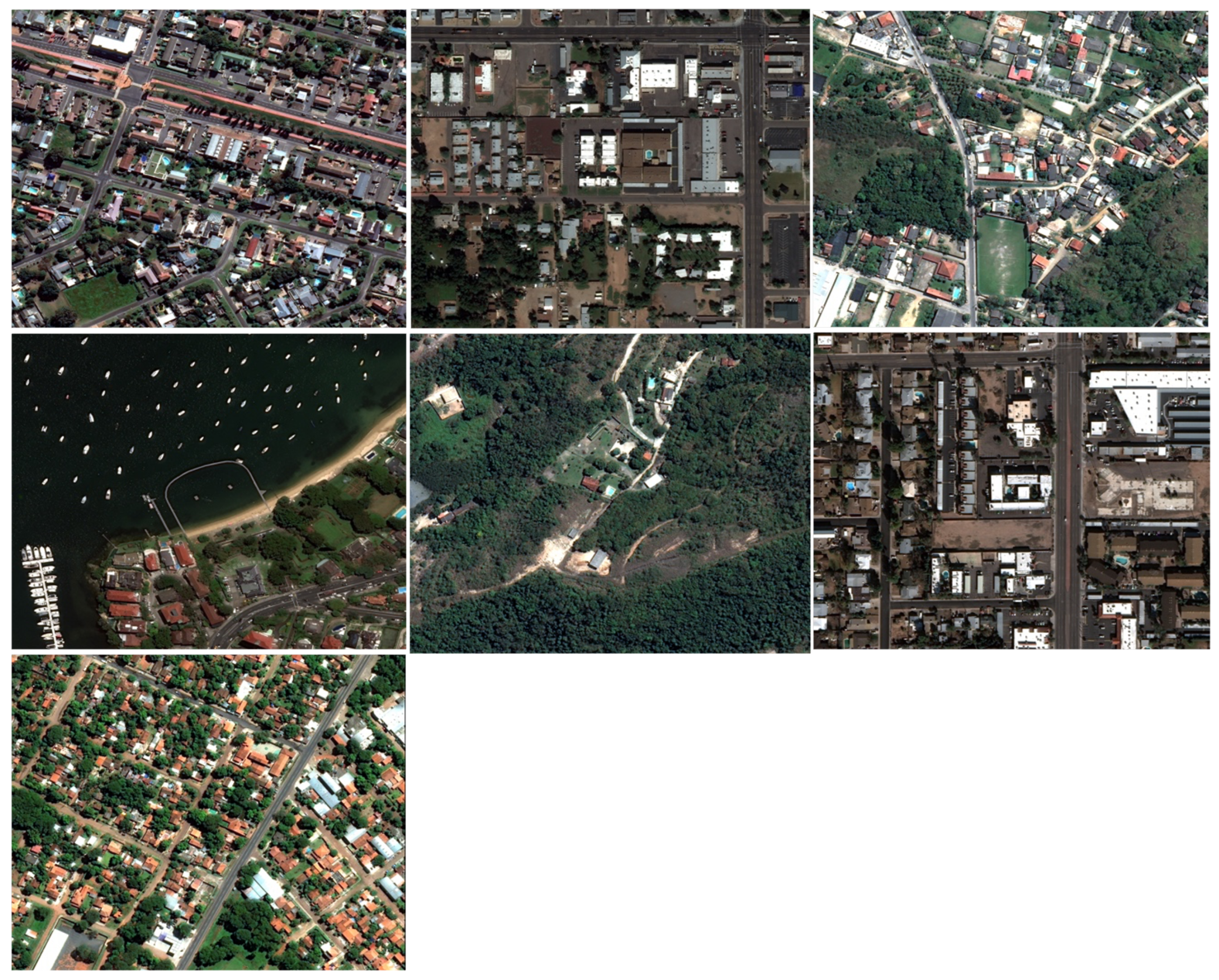
Figure A5.
Image from fountain class that was misclassified by Inception v3 containing blue object.
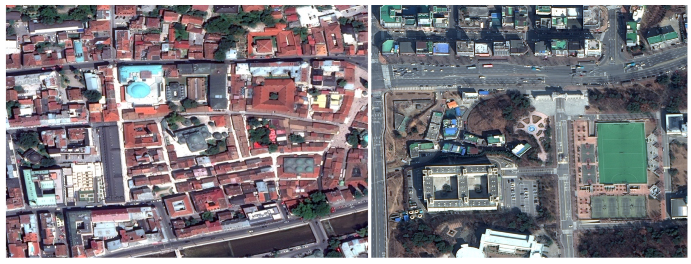
Figure A6.
Images from swimming pool class misclassified by the Magnifying Network.
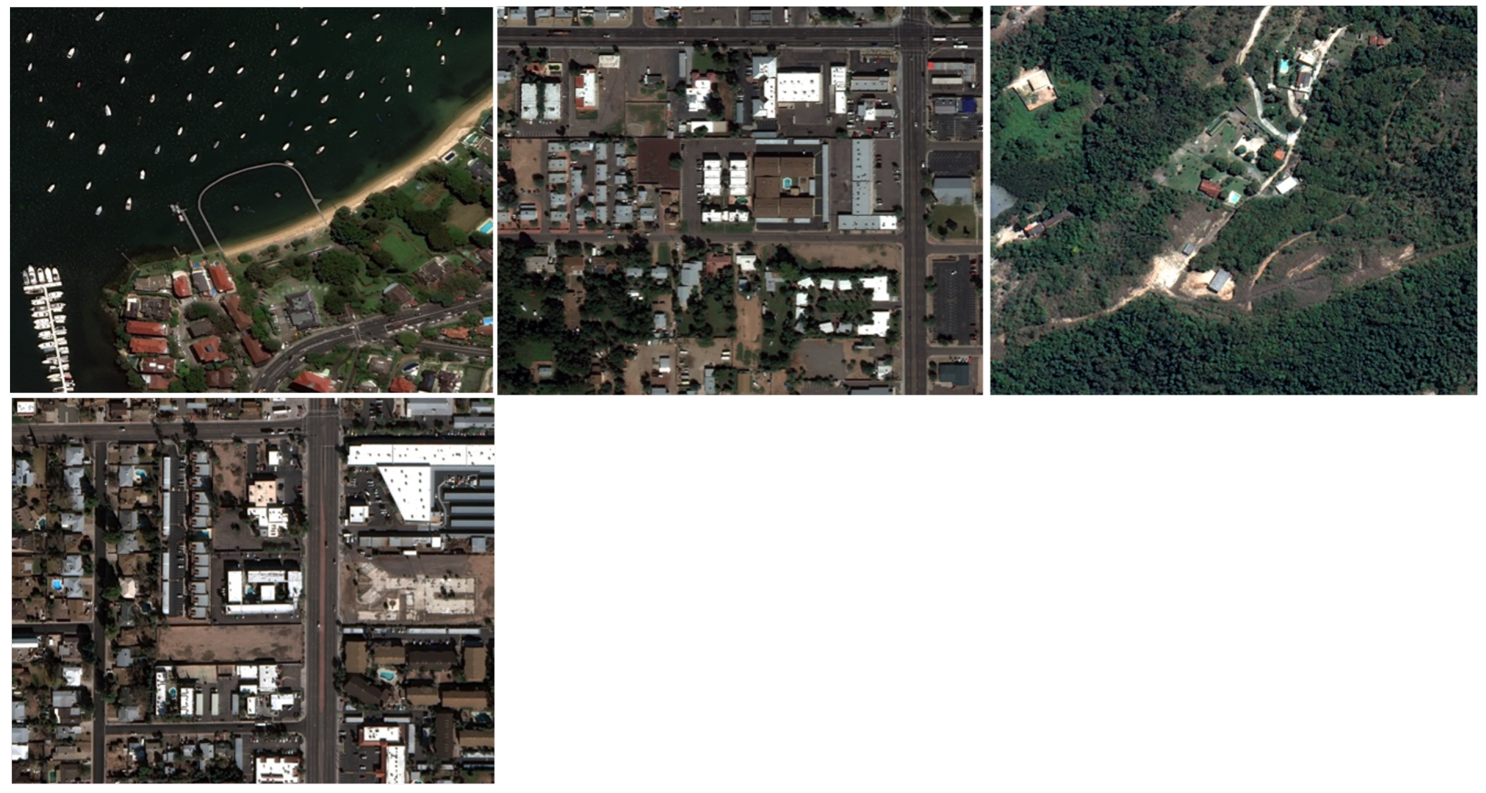
Figure A7.
Images from fountain class misclassified by the Magnifying Network.
References
- Chakraborty, S. Remote sensing and GIS in environmental management. In Environmental Management: Issues and Concerns in Developing Countries; Springer: Cham, Switzerland, 2021; pp. 185–220. [Google Scholar]
- Manfré, L.; Hirata, E.; Silva, J.; Shinohara, E.; Giannotti, M.; Larocca, A.; Quintanilha, J. An analysis of geospatial technologies for risk and natural disaster management. ISPRS Int. J. Geo-Inf. 2012, 1, 166–185. [Google Scholar] [CrossRef] [Scilit]
- Segarra, J. Satellite Imagery in Precision Agriculture. In Digital Agriculture: A Solution for Sustainable Food and Nutritional Security; Springer: Cham, Switzerland, 2024; pp. 325–340. [Google Scholar]
- Hoffman, C.; Lemper, M. Satellite Applications for Sustainable Urban Planning and Management. In Proceedings of the Satellite-Based Earth Observation: Trends and Challenges for Economy and Society; Springer: Cham, Switzerland, 2018; pp. 147–156. [Google Scholar]
- Park, H.; Kim, N.; Park, S.; Choi, J. Sharpening of WorldView-3 satellite images by generating optimal high-spatial-resolution images. Appl. Sci. 2020, 10, 7313. [Google Scholar] [CrossRef] [Scilit]
- Drusch, M.; Del Bello, U.; Carlier, S.; Colin, O.; Fernandez, V.; Gascon, F.; Hoersch, B.; Isola, C.; Laberinti, P.; Martimort, P.; et al. Sentinel-2: ESA’s optical high-resolution mission for GMES operational services. Remote Sens. Environ. 2012, 120, 25–36. [Google Scholar] [CrossRef] [Scilit]
- Gleyzes, M.; Perret, L.; Kubik, P. PLEIADES system architecture and main performances. Int. Arch. Photogramm. Remote Sens. Spat. Inf. Sci. 2012, 39, 537–542. [Google Scholar] [CrossRef] [Scilit]
- Dimitriou, N.; Arandjelovic, O.; Harrison, D. Magnifying Networks for Histopathological Images with Billions of Pixels. Diagnostics 2024, 14, 524. [Google Scholar] [CrossRef] [Scilit]
- Bakhtiarnia, A.; Zhang, Q.; Iosifidis, A. Efficient High-Resolution Deep Learning: A Survey. ACM Comput. Surv. 2024, 56, 1–35. [Google Scholar] [CrossRef] [Scilit]
- Gupta, R.; Li, S.; Zhu, T.; Malik, J.; Darrell, T.; Mangalam, K. xT: Nested Tokenization for Larger Context in Large Images. arXiv 2024, arXiv:2403.01915. [Google Scholar] [CrossRef] [Scilit]
- Li, W.; He, C.; Fang, J.; Zheng, J.; Fu, H.; Yu, L. Semantic segmentation-based building footprint extraction using very high-resolution satellite images and multi-source GIS data. Remote Sens. 2019, 11, 403. [Google Scholar] [CrossRef] [Scilit]
- Liu, Y.; Ren, Q.; Geng, J.; Ding, M.; Li, J. Efficient patch-wise semantic segmentation for large-scale remote sensing images. Sensors 2018, 18, 3232. [Google Scholar] [CrossRef] [Scilit]
- Audebert, N.; Le Saux, B.; Lefèvre, S. Segment-before-detect: Vehicle detection and classification through semantic segmentation of aerial images. Remote Sens. 2017, 9, 368. [Google Scholar] [CrossRef] [Scilit]
- Jenkinson, E.; Arandjelovic, O. Whole Slide Image Understanding in Pathology: What Is the Salient Scale of Analysis? BioMedInformatics 2024, 4, 489–518. [Google Scholar] [CrossRef] [Scilit]
- Dimitriou, N. Computational Analysis of Tissue Images in Cancer Diagnosis and Prognosis: Machine Learning-Based Methods for the Next Generation of Computational Pathology. Ph.D. Thesis, University of St Andrews, St Andrews, UK, 2023. [Google Scholar]
- Li, B.; Li, Y.; Eliceiri, K. Dual-stream multiple instance learning network for whole slide image classification with self-supervised contrastive learning. In Proceedings of the IEEE/CVF Conference on Computer Vision and Pattern Recognition, Nashville, TN, USA, 20–25 June 2021; pp. 14318–14328. [Google Scholar]
- Dimitriou, N.; Arandjelović, O.; Caie, P.D. Deep Learning for Whole Slide Image Analysis: An Overview. Front. Med. 2019, 6, 264. [Google Scholar] [CrossRef] [Scilit]
- Muhammad, U.; Hoque, M.Z.; Wang, W.; Oussalah, M. Patch-Based Discriminative Learning for Remote Sensing Scene Classification. Remote Sens. 2022, 14, 5913. [Google Scholar] [CrossRef] [Scilit]
- Wang, X.; Xu, H.; Yuan, L.; Dai, W.; Wen, X. A Remote-Sensing Scene-Image Classification Method Based on Deep Multiple-Instance Learning with a Residual Dense Attention ConvNet. Remote Sens. 2022, 14, 5095. [Google Scholar] [CrossRef] [Scilit]
- Wang, X.; Yan, Y.; Tang, P.; Bai, X.; Liu, W. Revisiting multiple instance neural networks. Pattern Recognit. 2018, 74, 15–24. [Google Scholar] [CrossRef] [Scilit]
- Wang, Q.; Liu, S.; Chanussot, J.; Li, X. Scene classification with recurrent attention of VHR remote sensing images. IEEE Trans. Geosci. Remote Sens. 2019, 57, 1155–1167. [Google Scholar] [CrossRef] [Scilit]
- Xu, K.; Huang, H.; Deng, P.; Li, Y. Deep Feature Aggregation Framework Driven by Graph Convolutional Network for Scene Classification in Remote Sensing. IEEE Trans. Neural Netw. Learn. Syst. 2021, 33, 5751–5765. [Google Scholar] [CrossRef] [Scilit] [PubMed]
- Huang, Q.; Jiang, F.; Huang, C. Remote sensing scene classification with relation-aware dynamic graph neural networks. Eng. Appl. Artif. Intell. 2025, 150, 110513. [Google Scholar] [CrossRef] [Scilit]
- Yang, Y.; Tang, X.; Cheung, Y.M.; Zhang, X.; Jiao, L. SAGN: Semantic-Aware Graph Network for Remote Sensing Scene Classification. IEEE Trans. Image Process. 2023, 32, 1011–1025. [Google Scholar] [CrossRef] [Scilit]
- Chen, R.J.; Chen, C.; Li, Y.; Chen, T.Y.; Trister, A.D.; Krishnan, R.G.; Mahmood, F. Scaling Vision Transformers to Gigapixel Images via Hierarchical Self-Supervised Learning. In Proceedings of the IEEE/CVF Conference on Computer Vision and Pattern Recognition (CVPR), New Orleans, LA, USA, 18–24 June 2022; pp. 16144–16155. [Google Scholar]
- Christie, G.; Fendley, N.; Wilson, J.; Mukherjee, R. Functional map of the world. In Proceedings of the IEEE Conference on Computer Vision and Pattern Recognition, Salt Lake City, UT, USA, 18–23 June 2018; pp. 6172–6180. [Google Scholar]
- Kingma, D. Adam: A method for stochastic optimization. arXiv 2014, arXiv:1412.6980. [Google Scholar]
- Dozat, T. Incorporating Nesterov Momentum into Adam. In Proceedings of the International Conference on Learning Representations (ICLR), Workshop Track, San Juan, PR, USA, 2–4 May 2016; pp. 1–4. [Google Scholar]
- Loshchilov, I. Decoupled weight decay regularization. arXiv 2017, arXiv:1711.05101. [Google Scholar]
- Tieleman, T.; Hinton, G. Lecture 6.5—RMSprop: Divide the gradient by a running average of its recent magnitude. COURSERA Neural Netw. Mach. Learn. 2012, 4, 26. [Google Scholar]
- Bottou, L. Large-Scale Machine Learning with Stochastic Gradient Descent. In Proceedings of the International Conference on Computational Statistics; Physica-Verlag HD: Heidelberg, Germany, 2010. [Google Scholar]

Disclaimer/Publisher’s Note: The statements, opinions and data contained in all publications are solely those of the individual author(s) and contributor(s) and not of MDPI and/or the editor(s). MDPI and/or the editor(s) disclaim responsibility for any injury to people or property resulting from any ideas, methods, instructions or products referred to in the content. |
© 2026 by the authors. Licensee MDPI, Basel, Switzerland. This article is an open access article distributed under the terms and conditions of the Creative Commons Attribution (CC BY) license.