


Abstract
The increasing penetration of distributed energy resources requires battery energy storage systems (BESSs) to be scheduled economically while preserving network security and accounting for battery-life consumption. This work’s primary technical contribution is an integrated, degradation-aware framework for coordinated day-ahead active–reactive power dispatch of multiple BESS units in active distribution networks. The formulation minimizes grid-energy purchases, PV and BESS operation and maintenance costs, and monetized cycling and calendar degradation while enforcing nonlinear AC power-flow equations, voltage and branch-current limits, converter apparent-power capability, non-ideal state-of-charge dynamics, and terminal-energy requirements. Each candidate 24-h SoC trajectory is processed through a Rainflow-based semi-empirical aging model, allowing degradation to be included directly in the fitness evaluation. SELGO is employed as the optimization engine and coupled with a parallel successive-approximation AC power-flow evaluator. The framework is assessed through 100 independent executions under deterministic operating conditions and 100 stochastic demand and PV-generation scenarios in a modified 33-bus system, together with 100 stochastic scenarios in a modified 69-bus system. SELGO is compared with AJAYA, GA, MVO, PSO, and TDE under equivalent models, constraints, scenarios, and parameter-tuning conditions. Among the evaluated methods, SELGO yields the smallest mean operating cost for each of the three analyzed cases, reducing the corresponding base costs by 2.2015%, 2.4017%, and 3.0108%, respectively, while satisfying voltage, thermal, converter, and inter-temporal BESS constraints. The cumulative ablation analysis also supports the conditional benefit of the complete SELGO architecture. Across the analyzed cases, cycling intensity ranges from 0.7690 to 0.8386 EFC/day and daily aging from to day−1. Under the repeated-day assumption, the 80% SoH threshold is reached after 5.9756–6.9238 years, whereas the corresponding interval for 70% SoH is 10.8433–12.5639 years; these values are intended for comparative aging interpretation rather than as field-life predictions. The results show that the framework identifies low-cost, AC-feasible schedules while explicitly quantifying the associated battery-life consumption.
1. Introduction
1.1. Problem Description
Growing deployment of distributed energy resources (DERs) is reshaping conventional distribution grids and giving rise to active distribution networks (ADNs) with decentralized generation and increasingly bidirectional power flows [1]. Although this transition supports decarbonization and greater use of renewable resources, the variability of photovoltaic and other distributed generation sources does not always coincide with demand patterns. This mismatch can intensify net-load fluctuations, reverse power flows, localized congestion, voltage deviations, and thermal stress on distribution feeders [2,3,4]. Consequently, maintaining secure and economical operation becomes increasingly difficult as renewable penetration and network utilization grow [5].
Battery energy storage systems (BESSs) provide a flexible alternative for mitigating these operational challenges because they can rapidly absorb or inject power according to system conditions [4,6]. Through coordinated charging, discharging, and converter-based reactive-power support, BESS units can reduce operating costs, alleviate feeder loading, improve voltage regulation, and facilitate renewable-energy integration [7,8]. However, these benefits depend strongly on the quality of the adopted scheduling strategy, since storage decisions are coupled across time through state-of-charge dynamics and must simultaneously respect battery, converter, voltage, and branch-current constraints.
Therefore, optimal BESS scheduling constitutes a nonlinear and high-dimensional problem in which economic performance cannot be considered independently of AC network feasibility and battery usage. Simplified energy-management formulations may produce attractive operating costs while overlooking network violations, converter limitations, or excessive cycling stress. Advanced optimization frameworks are thus required to coordinate active and reactive BESS power over the complete scheduling horizon while preserving technical feasibility and accounting for the operational impact of battery degradation [2,9].
1.2. Literature Review
Recent studies on optimal BESS operation have addressed the problem through short-term energy management, multi-objective optimization, mathematical programming, and computational-intelligence techniques. These approaches differ mainly in their scheduling horizons, network representations, objective functions, uncertainty treatments, and levels of coordination between storage systems and other distributed energy resources.
Regarding short-term microgrid operation, Nguyen et al. [10] develops a Simulink-based model predictive control framework in which demand, photovoltaic generation, wind generation, and electricity tariff data are updated at 15 min intervals. At each interval, the coyote optimization algorithm determines the BESS active-power reference that minimizes the electricity purchased from the main grid. The method is compared with PSO and a power-balance-based heuristic, obtaining the highest cost reduction among the evaluated strategies. Similarly, Polanco Vásquez et al. [11] combines model predictive control, multi-objective optimization, and an automated decision tool to simultaneously minimize the operating cost and emissions of a microgrid. The receding-horizon formulation is repeatedly updated using new information, and its performance is examined under both ideal forecasts and prediction errors.
Other studies have jointly examined BESS planning and operation over longer time horizons. In [12], the allocation of distributed generation and battery storage, their annual active-power profiles, and the power-factor profiles of controllable and non-controllable generation are optimized simultaneously. The formulation seeks to reduce yearly losses and the energy exchanged with the upstream grid using hourly load, photovoltaic, and wind-generation data. Its solution combines metaheuristic optimization, power-system simulation, and artificial neural networks for the subsequent control of the optimized profiles. In turn, da Silva et al. [4] formulates a multi-period optimal power-flow model for the simultaneous siting and operation of one, two, or three BESS units in a photovoltaic-rich 33-bus distribution system. The model is solved over a 168-h horizon using AMPL and Knitro, with the objective of minimizing energy losses while improving the voltage profile and smoothing the generation curve observed at the substation.
AC-network-constrained BESS scheduling has also been studied through deterministic mathematical programming and parallel metaheuristic methods. In [13], a nonlinear programming model is developed to optimize BESS operation according to three separate objectives: operational cost, energy losses, and emissions. The model is solved using SNOPT in GAMS (version 54.6.1) and is evaluated in a grid-connected 33-bus system and a stand-alone 27-bus network using demand and photovoltaic generation data from two Colombian regions. Its results are compared with the Chu–Beasley genetic algorithm, PSO, the vortex search algorithm, and the ant lion optimizer. More recently, Sanin-Villa et al. [14] integrates a parallel Multi-Verse Optimizer with a successive-approximation power-flow evaluator for BESS scheduling in grid-connected and islanded AC microgrids. The proposed framework minimizes energy losses and emissions while verifying voltage stability and the technical feasibility of the resulting operating schedules.
Recent multi-objective formulations have further emphasized the coordinated operation of renewable generation and storage. In [15], decentralized PV and BESS units are managed in a modified 33-bus system using SPEA2. The formulation simultaneously minimizes power losses and voltage deviation, maximizes the financial return of the distribution network operator, and reduces energy imports from the main grid. The numerical assessment considers four PV systems and two BESS units and reports improvements in the technical and economic indicators relative to the reference operating condition. Meanwhile, Vega et al. [16] presents a 24-h economic dispatch framework for the coordinated operation of wind turbines and BESS units in distribution microgrids. The formulation determines active- and reactive-power references while enforcing AC network constraints, BESS SoC limits, and converter apparent-power capability in grid-connected and isolated modes. A genetic algorithm is compared with PSO and MVO through 100 independent executions, considering objective quality, result dispersion, execution time, and network feasibility.
Despite recent progress in BESS scheduling, economic performance, AC network feasibility, uncertainty, computational efficiency, and battery degradation are still commonly addressed through separate or partially integrated formulations. To bridge this gap, the present work combines coordinated BESS P–Q dispatch, nonlinear AC constraints, non-ideal SoC dynamics, scenario-based demand and PV uncertainty, parallel candidate evaluation, consistent multi-algorithm benchmarking, and cumulative operator-level ablation within a unified framework. Moreover, cycling and calendar degradation are monetized for every candidate SoC trajectory, directly linking short-term operating-cost minimization with battery-life consumption.
Battery degradation modeling in BESS operation is application dependent, since the required aging representation varies with the operating profile, scheduling horizon, and level of physical detail. The literature spans aggregate EFC/throughput models, empirical and semi-empirical cycle-resolved formulations, data-driven approaches, temperature-coupled/electro-thermal models, and physics-based electrochemical representations [17,18]. Simplified models reduce data, parameterization, and computational requirements but retain less information on cycle-specific and operating stresses, whereas more detailed formulations can represent additional effects such as DoD, SoC, C-rate, calendar aging, temperature dynamics, or internal battery states. Accordingly, model selection reflects an application-specific trade-off between degradation detail and implementation requirements rather than a universal hierarchy of fidelity.
This trade-off is evident across the stationary-storage applications relevant to power-system integration. PV–BESS studies employ approaches ranging from EFC/throughput accounting to Rainflow-based partial-cycle treatment and cycling–calendar or multi-stress formulations [19,20,21,22]. Microgrid and day-ahead EMS studies additionally consider single- and multi-factor semi-empirical models, nonlinear Rainflow-based aging, and data-driven formulations [18,23,24,25]. For standalone utility-scale BESS and grid services, temperature-coupled/electro-thermal and physics-based electrochemical models have also been adopted when thermal dynamics or internal battery states require explicit representation [26,27,28,29,30]. Over longer planning horizons, linear, piecewise-linear, cycle-counting, and physics-based equivalent-circuit models are used to balance degradation representation with multi-period computational requirements [31,32,33,34]. Table 1 consolidates these representative approaches, their principal input requirements, and their application-oriented modeling trade-offs.
Table 1.
Representative battery-degradation approaches for stationary BESS applications, highlighting their required inputs and application-oriented modeling trade-offs reported in the literature.
Based on the application-oriented comparison in Table 1, the present study is positioned in the integrated PV–BESS active-distribution-network setting under day-ahead supervisory scheduling. In this context, degradation must be evaluated repeatedly from each candidate 24-h SoC trajectory while AC-network feasibility is simultaneously assessed. A basic EFC/throughput model would not provide the trajectory detail required here because it aggregates battery use without resolving cycle depth and partial-cycle structure, whereas electro-thermal or electrochemical formulations would introduce extra requirements for thermal and electrochemical states, cell-specific parameters, and associated data beyond the scope of the present scheduling problem. Accordingly, a Rainflow-based semi-empirical cycling–calendar model is adopted as an intermediate modeling level: it resolves complete and partial cycles and accounts for DoD, mean SoC, and calendar aging, while temperature is evaluated under the fixed 298.15 K reference assumption. This choice therefore preserves trajectory-dependent aging information without requiring higher-fidelity state propagation for every optimization candidate [17,18,23,30].
This balance is particularly relevant because degradation is monetized within the operating objective, so the selected aging representation directly links trajectory-dependent battery use with the economic assessment of each candidate schedule.
1.3. Problem Statement and Main Contributions
This study considers coordinated day-ahead operation of multiple BESS units in photovoltaic-rich active distribution networks with time-varying demand. The optimization minimizes total daily operating expenditure by accounting for grid-energy procurement, PV and BESS O&M, and monetized battery aging. The formulation is strongly coupled because active- and reactive-power decisions interact over time through non-ideal SoC evolution, and each hourly state must respect the nonlinear AC equations, nodal-voltage and branch-current bounds, converter capability, and terminal-energy conditions. Battery aging is also trajectory dependent rather than determined solely by aggregate energy exchange. Hence, simplified EMS formulations can appear economical while producing electrically inadmissible schedules or understating battery-life consumption.
The framework targets supervisory coordination at the DMS/EMS level. It supplies hourly active- and reactive-power references for the BESS converters, while local controllers retain responsibility for fast voltage regulation, protection, switching, and device-level tracking. Each candidate schedule is repaired according to the BESS operating constraints and evaluated through a successive-approximation AC power flow. Its complete SoC trajectory is then processed by the degradation model, and the resulting cycling and calendar aging cost is incorporated into the candidate fitness. Therefore, the final schedules can be interpreted as degradation-aware and AC-feasible supervisory set-points.
The specific contributions developed in this study are:
- Integrated degradation-aware AC formulation: A unified multi-period scheduling model jointly accounts for purchased grid energy, PV operation, BESS operation, and monetized storage aging. The formulation includes charging and discharging efficiencies, self-discharge, SoC bounds, initial and terminal energy conditions, nonlinear AC power-flow equations, voltage limits, and branch-current constraints.
- Coordinated BESS active–reactive operation: Each candidate solution represents the full 24-h BESS-fleet P–Q schedule. Active and reactive power are coupled through the converter apparent-power capability, allowing the storage units to perform energy shifting and voltage-support actions without violating their converter or inter-temporal operating limits.
- Parallel SELGO–SA solution framework: SELGO performs the optimization search, and parallel candidate evaluation invokes the successive-approximation power-flow evaluator. The complete SELGO architecture combines leader-guided pursuit, population reorganization, adaptive renewal, and late-stage pattern-search refinement. A cumulative ablation study is also conducted to quantify the conditional marginal improvement obtained as these complementary mechanisms are progressively activated.
- Consistent benchmarking under deterministic and stochastic operation: The methodology is assessed through 100 independent executions in the deterministic modified 33-bus system, 100 stochastic demand and PV-generation scenarios in the same network, and another 100 stochastic scenarios in the modified 69-bus system. SELGO is compared with AJAYA, GA, MVO, PSO, and TDE under identical network models, economic coefficients, BESS limits, operating scenarios, and parameter-tuning conditions. The assessment includes best and average cost, dispersion, computational effort, statistical significance, and electrical feasibility.
- Battery-aging and asset-level interpretation: The complete SoC trajectory of every candidate schedule is evaluated through rainflow-based cycling degradation and calendar aging, and the resulting daily degradation factor is included in the objective function. The final solutions are additionally reported using throughput, daily EFC, daily aging, projected SoH, and threshold-based lifetime measures under the repeated-day operating assumption. This analysis clarifies why battery-life consumption depends on cycle depth, normalized cycling intensity, mean SoC, and trajectory shape rather than only on the processed energy.
The primary technical contribution of this work is the integrated degradation-aware scheduling framework, which combines degradation-aware economics, AC-feasible BESS P–Q scheduling, parallel metaheuristic optimization, uncertainty assessment, consistent benchmarking, and operator-level validation. Within this framework, SELGO provides the algorithmic contribution and serves as the optimization engine used to solve the resulting scheduling problem.
Table 2 provides a comparative overview of representative BESS-operation approaches and highlights the scope covered by the proposed methodology. Most previous studies incorporate only a subset of the relevant operational features. In contrast, the framework considered here jointly addresses AC-network feasibility, voltage and thermal limits, uncertainty, converter reactive-power capability, systematic algorithm comparison, and the economic effect of battery aging within the operating-cost objective.
Table 2.
Comparison of representative BESS-operation studies for distribution-network and microgrid applications.
1.4. Document Organization
The manuscript is arranged into five subsequent sections. Section 2 develops the day-ahead degradation-aware formulation, covering the daily cost function, the AC network equations, operating bounds on voltages and branch currents, coordinated active–reactive BESS limits, non-ideal SoC evolution across time, and the cycling/calendar aging terms included in the optimization. Section 3 explains the SELGO–SA computational procedure, from the P–Q schedule representation and feasibility correction to the search mechanisms, parallel evaluation of individuals, SA-based network fitness calculation, and parameter calibration for SELGO and the comparison algorithms.
Section 4 specifies the modified 33- and 69-bus feeders and the associated electrical, PV, storage, economic, and degradation data. It also establishes the deterministic and stochastic conditions used to examine repeatability, uncertainty effects, and behavior as feeder complexity increases. Section 5 analyzes the numerical outcomes for deterministic operation of the 33-bus feeder and stochastic operation of both test networks. The discussion covers cost results, dispersion, execution time, statistical evidence, convergence, AC-feasibility indicators, BESS P–Q schedules, SoC profiles, aging metrics, cumulative SELGO ablation, and the comparison between degradation-aware and degradation-unaware scheduling. Section 6 closes the paper by consolidating the main findings and discussing academic and industrial implications, possible methodological extensions, study limitations, and future research.
2. Mathematical Model for Degradation-Aware Day-Ahead BESS Scheduling
The proposed day-ahead model is cast as a nonlinear programming (NLP) model over 24 hourly intervals. It determines how the BESS fleet is coordinated in an ADN subject to time-varying demand and distributed photovoltaic generation (PV DG). The optimization seeks a minimum-cost daily schedule while enforcing the AC network equations, equipment operating limits, converter constraints, and inter-temporal energy requirements across the BESS fleet.
The notation uses for network nodes, for distribution lines, for scheduling periods, for PV DG units, and for BESS units. At node i, the subsets and identify the connected PV DG and BESS units, respectively. The duration assigned to one scheduling interval is . In this formulation, PV DG units follow maximum power point tracking (MPPT), so their active-power production tracks the available solar resource. The BESS converters are modeled as controllable devices capable of exchanging real and reactive power, subject to the converter apparent-power capability.
2.1. Daily Operating-Cost Objective
The objective function seeks the minimum daily operational cost of the ADN across the scheduling horizon. This cost includes the energy supplied by conventional generators, the O&M expenditures related to PV DG and BESS operation, plus the equivalent monetary cost of the degradation produced by daily operation of the storage fleet. Accordingly, the optimization problem is expressed as
Equation (1) represents the complete operating-cost objective adopted in this study. Its first term corresponds to the energy delivered from conventional sources, where is the energy cost coefficient at hour h and denotes conventional active-power injection at node i for period h. Therefore, represents the energy supplied within that interval. The next term represents the PV DG operation and maintenance cost, where denotes the corresponding cost coefficient and is the power produced by PV unit p during period h. The third component captures the BESS operation and maintenance expenditure, where weights BESS energy throughput and denotes the magnitude of active-power exchange for BESS b. This absolute value allows the same signed power variable to account for energy transfer in either direction.
The final term introduces the BESS degradation cost directly into the optimization problem. The product represents the replacement cost of BESS b, since denotes battery cost per energy unit and denotes nominal energy capacity. This replacement cost is then weighted using , the degradation factor assigned to day d, which is obtained from the lithium-ion aging model and represents the equivalent degradation fraction assigned to the optimized daily operation. Hence, the degradation term converts the physical aging effect of the BESS into an equivalent daily monetary cost.
2.2. Set of Operating Constraints
Active-power balance for every node and period is written in rectangular AC voltage coordinates as
In Equation (2), represents node i’s active demand during period h. The variables , , and denote active-power contributions from conventional generation, PV DG, and the BESS, respectively. The BESS variable is signed: positive values correspond to discharging and network injection, whereas negative values correspond to charging and absorption from the network. Thus, gives the net BESS active-power contribution at node i. The right-hand side computes the net active-power contribution of incident branches from the rectangular voltage and current components through the incidence coefficient .
This signed BESS power variable is interpreted according to the following convention:
Thus, charging, idle operation, and discharging are represented by the same signed active-power variable. For , the BESS absorbs active power and its stored energy increases; for , it injects active power and its stored energy decreases; and for , it remains idle from the active-power perspective. Hence, the model excludes simultaneous charging and discharging because no independent charging and discharging variables are used.
Reactive-power balance is imposed as
In Equation (4), denotes reactive demand at node i during period h, is the conventional-source reactive contribution, and is the BESS-converter reactive exchange. This variable provides converter-based voltage support without changing stored battery energy. Positive injects reactive power into the network, whereas negative absorbs it. Since PV DG units are operated under MPPT conditions, their contribution is represented only through the active-power injection in Equation (2).
For line l, current is represented through its real and imaginary components as
where the parameters and are branch series resistance and reactance quantities for line l, respectively. Equations (5) and (6) map the nodal voltage variables into branch-current components based on network connectivity and the line impedance.
The voltage and current magnitudes are defined as
A nodal voltage magnitude shall remain within the permitted operating range:
Each distribution-line current is required to remain below its thermal rating:
Constraints (9) and (10) ensure secure network operation by avoiding voltage violations and conductor overloading during the optimized daily dispatch.
Active- and reactive-power injections of the conventional generators are bounded according to
PV DG active-power production is computed from solar-resource availability as
where is the installed capacity of PV unit p and is a normalized solar-availability factor for period h. This equation represents MPPT operation, where the PV active-power generation tracks the available solar resource.
Each BESS active-power exchange is constrained by its available charging and discharging capability:
The BESS active-power bounds are obtained using rated energy together with the specified charging and discharging times:
Accordingly, is the negative charging limit, while is the positive discharging limit.
The permitted reactive-power range of each BESS converter is specified by
The rated-power capability of each BESS converter is enforced through
Here, denotes the converter apparent-power rating. Equation (17) links the active and reactive exchanges through this common rating. Therefore, when a BESS charges or discharges close to its active-power limit, the residual unused converter margin for reactive support is reduced; when the active-power exchange is low, a larger reactive contribution can be provided without surpassing the converter rating.
The BESS energy-state recursion includes charge efficiency, discharge efficiency, and self-discharge:
In Equation (18), gives the state of charge reached by BESS b at period h, is the self-discharge rate, and converts exchanged power into normalized energy variation. The direction-dependent efficiency factor is defined from the sign of as
where and denote the respective charging and discharging efficiencies. With the adopted sign convention, charging corresponds to and increases the SoC after considering , while discharging corresponds to and decreases the SoC considering .
The energy normalization factor is expressed as
Initial and terminal SoC requirements are imposed through
Constraint (21) enforces the endpoint requirements on the BESS energy trajectory, guaranteeing cyclic daily operation and avoiding artificial energy gains at the end of the horizon.
The BESS SoC must remain inside its permitted operating window:
Constraint (22) prevents operation beyond the upper and lower SoC limits, preserving admissible BESS operation throughout the scheduling horizon.
2.3. Battery Aging Model
A BESS aging term in the objective is computed from a semi-empirical lithium-ion battery aging model based on cycling and calendar degradation mechanisms [26,36]. The daily degradation factor assigned to each BESS is written as
where is the daily degradation factor used in the objective function, while and are the two aging contributions assigned to BESS b for day d, respectively.
The degradation model uses the optimized SoC trajectory of each BESS:
Cycling aging is obtained by applying Rainflow analysis to the daily SoC trajectory. This analysis partitions the SoC profile into equivalent full and incomplete charge–discharge events. The cycling degradation component is calculated as
where denotes the count of Rainflow-identified cycle events for BESS b, is the count of event r, and , , and act as multipliers for depth of discharge, mean SoC, and temperature effects, respectively.
For every event r, cycle depth and the mean SoC are computed as
The corresponding stress factors are defined as
Calendar aging accounts for time-dependent degradation caused by storage conditions during the daily horizon. It is modeled as
where denotes the calendar-aging coefficient and specifies the duration assigned to a full day using the time unit consistent with . The mean-SoC and temperature stress terms are represented by
where and are the average SoC and cell temperature for BESS b during day d.
These coefficients and operating parameters used in the lithium-ion degradation model are summarized in Table 3. The adopted degradation coefficients follow the lithium manganese oxide (LMO) battery parameterization reported in [26], where they were calibrated using experimental datasets covering calendar aging and cycle life. Therefore, the degradation assessment presented in this work is conditioned on this LMO-based parameterization.
Table 3.
Parameterization adopted for the lithium manganese oxide (LMO) degradation model.
A fixed BESS operating temperature of (25 °C) is assumed throughout the scheduling horizon. Temperature variations, particularly under high-power charge–discharge conditions, may materially influence lithium-ion battery aging. The fixed-temperature assumption is adopted for the following reasons [37,38,39]: (i) the degradation formulation is based on established lithium-ion aging models characterized under controlled thermal conditions; (ii) a common temperature provides a consistent basis for comparing the degradation effects of the evaluated schedules; (iii) this work focuses on degradation-aware day-ahead scheduling and coordinated active–reactive BESS dispatch rather than on electro-thermal battery dynamics; and (iv) modeling temperature evolution would require extra cell-specific thermal parameters and operating data beyond the present scope. Moreover, 25 °C is commonly adopted as a controlled or reference condition in battery-aging studies [38,39]. Consequently, the reported degradation results are conditional on this constant-temperature assumption, and future work should incorporate temperature-dependent aging and electro-thermal coupling under variable operating conditions.
Using the same degradation factor, the SoH associated with the optimized daily operation is estimated as
where and are empirical coefficients representing solid-electrolyte-interphase effects. This expression is used to translate the daily degradation factor to an equivalent SoH indicator.
Finally, an equivalent lifetime-to-threshold metric is obtained by assuming that the daily degradation factor corresponding to the analyzed 24-h SoC trajectory remains unchanged and is repeatedly applied until the selected SoH threshold is reached:
The associated equivalent lifetime expressed in years is
where counts the repeated operating days needed for BESS b to attain the selected threshold . This lifetime-to-threshold quantity serves as a comparative indicator of long-horizon aging intensity linked to the analyzed daily schedule, rather than as an accurate prediction of field service life, since capacity fade, future operating conditions, and changes in dispatch patterns are not propagated across successive days. The lifetime-to-threshold assessment assumes a fresh battery initially at 100% SoH, consistently with the complete SEI-based formulation adopted in the degradation model. For an already aged BESS, the current SoH would need to be introduced explicitly when estimating its remaining lifetime.
3. Optimization Framework and SELGO Search Procedure
The proposed optimization methodology addresses the day-ahead BESS problem through the Self-Evolving Lupine Group Optimizer (SELGO). Each wolf stores the hour-by-hour P and Q set-points assigned to the BESS units throughout the day-ahead horizon. The population therefore represents different possible dispatch trajectories, whose performance is evaluated according to the resulting operating cost while verifying the technical limits imposed by the formulation. For each wolf, network variables are computed period by period using the SA load-flow procedure [40]. These hourly calculations provide the electrical information required by the fitness evaluation, so economic quality is assessed together with network feasibility.
The proposed SELGO search process is structured through four complementary mechanisms:
- Leader-guided pursuit: each wolf moves according to its own search history and the location of the incumbent leader. This produces a directional pressure toward high-quality regions while retaining an individual contribution to the movement.
- Internal group reorganization: underperforming individuals are selectively modified through intra-population interactions. This mechanism redistributes the search effort inside the group, restores diversity, and avoids disrupting the best candidates already found by the population.
- Self-evolving renewal: when persistent stagnation is detected, weak individuals are replaced by feasible candidates generated around the current leader within a shrinking neighborhood. This mechanism introduces new search directions while preserving the guidance provided by the best solution found so far.
- Leader-centered pattern-search refinement: in the final part of the optimization process, and only when stagnation persists, the current leader is locally refined by perturbing a limited number of decision variables in positive and negative directions using a progressively reduced step size. Each trial solution is projected back into the feasible region and evaluated; if an improvement is found, the leader is updated and the improved candidate replaces the worst individual in the population. This stage enhances local exploitation and captures small improvements that may not be reached by the global population movements.
The proposed four-stage SELGO configuration uses iteration progress and stagnation status to determine operator activation. Pursuit establishes the dominant population movement, while reorganization and renewal restore alternative directions after progress weakens. The final local stage then concentrates on small coordinate corrections. In the present application, these complementary mechanisms are intended to address the search requirements imposed by the high dimensional BESS P-Q scheduling problem, including nonlinear AC-network feasibility, converter operating limits, and inter-temporal SoC coupling.
In this application, the rationale for combining the SELGO mechanisms follows from the structure of the scheduling problem rather than from the operators in isolation. Each candidate solution contains 144 time-indexed P–Q decision variables in the analyzed systems, whose effects are strongly coupled: the converter capability jointly constrains the P and Q commands, active-power decisions propagate through the inter-temporal SoC trajectory and terminal-energy requirement, and each hourly dispatch modifies the AC voltage and branch-current conditions of the network. Moreover, the degradation cost depends on the complete SoC trajectory, further coupling decisions across the scheduling horizon. Consequently, improving one subset of hourly variables may alter both the feasibility and economic effect of decisions in other periods, and a purely leader-driven search may become trapped in stagnant feasible neighborhoods before these coordinated adjustments are fully exploited. Under this problem structure, pursuit establishes the main search direction, whereas reorganization and renewal are activated under stagnation to introduce alternative search directions without globally restarting the population; the late-stage pattern search then targets small residual improvements around the best feasible schedule found so far. The operators are therefore not claimed to be mathematically indispensable in isolation; rather, their coordinated activation is designed to address the high dimensionality, nonlinear AC feasibility, converter P–Q coupling, inter-temporal SoC dependence, and trajectory-dependent degradation of the considered BESS scheduling problem. Their conditional marginal benefit is evaluated empirically through the cumulative ablation analysis in Section 5.4.
3.1. Representation and Initialization of Candidate Schedules
SELGO acts on a decision vector that contains the full active- and reactive-power schedule of the BESS fleet over the multi-period horizon. The vector is arranged in two consecutive parts: one part stores all active-power commands and the other stores the corresponding reactive-power commands.
For storage units and scheduling periods, each part contains entries. Hence, the dimension of the complete decision vector is
For wolf i, the two power blocks are grouped as
where contains the active-power trajectory and contains the reactive-power trajectory.
The active part is written as
and the reactive part as
Combining both blocks gives the complete schedule encoded by wolf i:
For the study considered here, three storage units are dispatched across hourly periods. This gives
decision variables.
The starting population is obtained by independently sampling every decision coordinate inside its admissible P–Q interval. For coordinate j of wolf i, the initialization rule is
with
where and delimit the feasible interval of decision coordinate j, and denotes the population size.
Collecting all initialized wolves produces
Every row of is a complete day-ahead BESS schedule, and each column collects one time-indexed command across all wolves. Before network evaluation, both power blocks in every row are processed by the repair procedure associated with the mathematical model so that the resulting schedule respects the BESS operating restrictions.
The repaired initial schedules are then evaluated with the SA power flow. The wolf with the lowest admissible fitness becomes the initial leader, denoted by . Section 3.3 describes the hourly network evaluation used for this purpose.
3.2. SELGO Search Operators
After initialization, one SELGO iteration may invoke four operators: leader pursuit together with group reorganization and self-evolving renewal, followed by a late pattern-search stage. Their activation depends on the iteration index and the current stagnation status, which allows the search to alternate between directional convergence, diversity restoration, and local refinement.
Let denote wolf i at iteration t. The mapping repairs a tentative vector with respect to the admissible BESS operating set , including active-power bounds, inter-temporal SoC conditions, and converter capability. AC-network constraints are subsequently checked by the SA evaluator.
Leader-guided pursuit. The pursuit stage assigns wolf i a displacement state . Its persistence is controlled by a coefficient that decreases linearly with the iteration count:
where and specify the initial and terminal values of the pursuit coefficient. Using this coefficient, the displacement for the next iteration is
Here, weights the contribution of the wolf’s own best record, weights the pull exerted by the current leader, and are independent random vectors. To prevent excessive coordinate changes, the resulting displacement is clipped component by component:
The vector sets the admissible displacement magnitude for each coordinate. The repaired trial position then becomes
The individual record of wolf i is replaced only when the new position provides a lower fitness value:
The index of the best member of the updated population is
and the incumbent leader is retained or replaced according to
Internal group reorganization. When the stagnation condition is active, a fraction of the least competitive wolves is considered for reorganization every iterations. For each selected member, an intermediate position is constructed as
The coefficient sets the reorganization amplitude, while and are two different wolves sampled from the current population. The intermediate vector is then combined coordinate-wise with the original wolf:
The parameter controls the probability of adopting a reorganized component; is the corresponding random draw, and forces at least one modified coordinate. After feasibility repair, the candidate is kept only when its fitness is lower than that of the selected wolf:
Self-evolving adaptive renewal. Persistent lack of improvement triggers renewal of a fraction of the weakest population members. The number selected for renewal is
Rather than drawing those replacements over the entire decision box, the renewal step samples them around the incumbent leader using a contracting radius:
In this expression, , is a random vector, is the all-ones vector, and and store the minimum and maximum admissible values for the complete P–Q vector. The renewal radius follows
where is the starting radius used by the renewal mechanism. Once repaired, the vectors are used to replace the selected weak wolves.
Leader-centered pattern-search refinement. When the search reaches its late stage and stagnation remains active, a coordinate neighborhood of the incumbent is examined. A subset is drawn at random. For every selected coordinate , two repaired probes are formed on opposite sides of the leader:
The vector selects coordinate d, while gives the probing distance on that coordinate. The better of the two local trials is obtained from
When the selected local trial improves the incumbent, the leader is updated through
If neither direction yields an improvement, the pattern-search step is contracted according to
A successful local trial is also inserted into the population in place of its worst member. This late operator is therefore used to resolve fine-scale improvements around the current feasible BESS P–Q schedule after the broader population movements have become less productive.
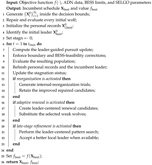
The search proceeds until is reached. At every iteration, tentative schedules are repaired, their fitness is computed with the SA evaluator, and the SELGO operators enabled by the current search state are applied. The feasibility criteria are those established in Section 2. Once the iteration limit is reached, the incumbent feasible P–Q schedule is reported, and Algorithm 1 summarizes the procedure.
3.3. Power-Flow-Based Fitness Evaluation
Within the proposed methodology, SELGO assigns a fitness value to every 24-h BESS P–Q schedule by coupling the optimization layer with the hourly ADN model. At interval , demand, MPPT PV production, and the BESS P and Q commands establish the network state to be solved. The resulting AC solution supplies nodal-voltage magnitudes, line-current values, together with the hourly cost terms required to build the daily objective and verify network limits.
| Algorithm 1: SELGO algorithm |
 |
The Successive Approximation (SA) technique [40] is adopted to calculate the hourly network state. Its iterative form provides the AC solution required by the fitness evaluator at each period, while the comparison with Newton–Raphson reported in [40] supports the adopted numerical choice. The demand-bus voltage update is
In (63), m indexes the internal SA loop; is the impedance block associated with demand buses, and couples the slack and demand subsets. denotes the slack-bus voltage at hour h, whereas is the conjugated net complex-demand vector. Each hourly solve begins from the prescribed slack condition and is stopped when the voltage mismatch falls below ; 1000 iterations are retained as the upper safeguard.
Once the hourly network state has converged, network feasibility is checked. Limits on BESS active power, inter-temporal SoC, initial/final SoC, and converter P–Q capability are handled by the encoding and repair stages. PV injections follow the MPPT profile, and nodal balance is satisfied by the solved AC equations. The battery-aging model in Section 2 then processes the 24-h SoC path associated with each candidate, combining cycling and calendar effects so that the corresponding monetized aging contribution enters . Therefore, only voltage-magnitude and branch-current excesses are added as post-power-flow penalties because these quantities are determined by the nonlinear network response.
The penalized fitness value is defined as
where denotes the daily operating-cost term and collects only penalties associated with network-limit violations. The corresponding current and voltage terms are computed as
and
Both coefficients are set to , so candidates that violate current or voltage limits become noncompetitive during selection. Thus, acts only as a constraint-handling term without adding another decision variable. After the SA evaluation, is passed back to SELGO as the score used to rank candidate schedules, favoring low-cost solutions that remain within the specified voltage and thermal bounds.
3.4. Benchmark Methods and Parameter Calibration
Five metaheuristics are used as comparison methods for SELGO: Adaptive JAYA (AJAYA) [41], Genetic Algorithm (GA) [42], Multi-Verse Optimizer (MVO) [43], Tri-Operator Differential Evolution (TDE) [44], and Particle Swarm Optimization (PSO) [45]. Together, these methods represent adaptive population learning, evolutionary recombination, universe-inspired search, differential operators, and swarm-memory dynamics.
Table 4 and Table 5 report the parameter values used in the final simulations. To avoid favoring an optimizer through manual parameter selection, every method was calibrated beforehand with the same external PSO procedure [45]. The calibration PSO served only as a parameter tuner and was not included as an additional competitor. Calibration used an identical objective definition, constraint set, and input dataset for every optimizer. The external PSO contained 30 particles and ran for 100 iterations; its acceleration coefficients were fixed at , with and . No execution-time cap was imposed, so the reported runtime reflects the search operations and tuned configuration of each method.
Table 4.
Tuning values used for the benchmark optimizers (AJAYA, GA, MVO, PSO, and TDE).
Table 5.
Parameter values adopted for SELGO in this study.
Because tuning determines and separately for every optimizer, their total candidate-evaluation counts are not forced to coincide. For method m, the objective-function budget is therefore reported as
where is the tuned population size of method m and is its tuned iteration limit. Every objective evaluation invokes the same 24-h SA-based network assessment. Consequently, the associated number of hourly network solves is
Table 6 lists both evaluation budgets for one 24-h optimization run. Wall-clock time is reported separately so that method-specific search effort can be distinguished from implementation and optimizer overhead. The runtime comparison should therefore be read together with the independently tuned evaluation counts rather than as an equal-budget experiment.
Table 6.
Per-run computational budgets for the 24-h optimization problem.
4. Test Networks and Study Setup
The following section introduces the network cases and operating data used for the numerical assessment of the proposed methodology. It also identifies the additional inputs required for evaluating the study objectives.
4.1. 33-Bus Distribution System
For repeated-run assessment, the modified 33-bus feeder provides the initial benchmark case. The electrical model follows the system reported in [13]. Figure 1 depicts the adopted topology and marks the connection nodes of the photovoltaic generators and storage units. Branch incidence, impedance data, nodal demands, and line thermal ratings required by the simulations are taken from [13].
Figure 1.
Topology of the 33-bus test feeder.
Table 7 compiles the feeder and distributed-resource data adopted for this case. The network contains 33 buses connected through 32 branches; its nominal voltage is 12.66 kV, the selected power base is 100 kVA, and admissible voltage magnitudes lie within p.u. PV generation is assigned to three locations: 13, 25, and 30; the corresponding ratings are 1125, 1320, and 999 kW. The storage units connect at locations 6, 14, and 31. Their energy ratings are 2000 kWh for the first unit, 1000 kWh for the second, and 1500 kWh for the third. Converter ratings, in the same sequence, are 400, 250, and 375 kVA.
Table 7.
Electrical, PV, and storage specifications adopted for the 33-bus case.
For the deterministic study, the 33-bus feeder uses representative demand and solar-production curves for Medellín, Colombia, adapted from [35]. The demand series originates from EPM operating records, while the solar resource is based on NASA irradiance information. Figure 2 shows the two 24-h input curves applied unchanged to every optimizer. Each method is run independently 100 times with these fixed inputs, allowing dispersion and repeatability to be assessed under the same operating case. PV production is represented in MPPT mode throughout the day.
Figure 2.
Daily deterministic demand and PV input curves adopted for the Medellín-based case, normalized to their respective reference values.
To complement the deterministic assessment, a stochastic assessment is also conducted for Medellín, Colombia. A 24-h reference operating condition, adapted from [35], is constructed using electricity-demand records provided by EPM and solar irradiance data from NASA. These two daily curves define the baseline from which the uncertainty scenarios are built. From these profiles, Monte Carlo sampling is used to construct 100 daily scenarios, with random hourly perturbations applied to both demand and PV generation. At each hour h of scenario s, the corresponding demand and PV-generation profile values are multiplied by the random factors and , respectively, where
Thus, both demand and PV generation can vary within of their corresponding hourly reference values. For the demand profile, the multiplicative scaling preserves the power factor and spatial distribution of the nodal loads. The network topology, BESS parameters, technical limits, and economic coefficients remain unchanged throughout the stochastic assessment. The degradation-aware AC-constrained model is solved separately for every resulting 24-h scenario. Therefore, the stochastic assessment optimizes every scenario separately rather than solving one stochastic problem with a common BESS schedule shared by all scenarios. For each optimization method, the reported operating-cost average is obtained from the 100 independently optimized scenario costs. Figure 3 and Figure 4 display the generated demand and PV scenario sets, respectively.
Figure 3.
Daily stochastic demand profiles generated through Monte Carlo sampling expressed as percentages of the reference demand.
Figure 4.
Daily stochastic PV-generation profiles generated through Monte Carlo sampling expressed as percentages of the reference PV generation.
4.2. 69-Bus Distribution System
For the larger feeder, the proposed methodology is applied to a modified 69-bus network based on [46]. Figure 5 depicts its topology and identifies the PV and BESS connection buses. The branch list, impedance parameters, nodal active/reactive demands, and thermal ratings used in the model follow [46].
Figure 5.
Topology adopted for the 69-bus benchmark feeder.
The 69-bus case uses the feeder topology and electrical parameters documented in [46]. Its common base settings 12.66 kV nominal voltage, 100 kVA base power, and voltage limits of p.u. match the configuration listed for the 33-bus case in Table 7. The PV ratings are 1320, 1125, and 999 kW for buses 16, 61, and 64, respectively. The storage locations are buses 62, 17, and 63. In that order, their energy ratings are 2000, 1000, and 1500 kWh, their converter ratings are 400, 250, and 375 kVA, and their nominal charge/discharge durations are 5, 4, and 4 h. The SoC range, boundary SoC values, efficiency during charging/discharging, and the self-discharge coefficient remain those specified in Section 4.1.
Only uncertainty-based operation is studied for this feeder. The Monte Carlo construction introduced for the 33-bus case is reused to form 100 operating scenarios from the Medellín reference curves, with simultaneous variability in load and photovoltaic output. Figure 3 and Figure 4 contain the corresponding scenario sets. They are used to test the proposed methodology when load and renewable output vary together.
4.3. Additional Considerations
Equation (1) is evaluated with the economic coefficients taken from [13]. The adopted values are USD/kWh for grid-energy purchases, USD/kWh for BESS O&M, USD/kWh for the battery-replacement coefficient, and USD/kWh for PV O&M. These coefficients are kept identical for both feeder cases. Hence, differences between the two cases reflect feeder configuration, DER placement, and the selected operating regime, while the economic assumptions remain unchanged.
Grid imports at the substation are priced with an hourly tariff signal. The corresponding coefficient is , where represents the normalized tariff factor for hour h. The same series is applied to both feeders, assigning time-dependent economic weights to imported energy. Figure 6 plots the normalized profile adapted from [35].
Figure 6.
Normalized hourly tariff coefficient , expressed as a percentage of the reference tariff and used to define the time-varying grid-energy purchase cost through .
The admissible SoC interval is set to 10–90%, consistent with a typical range used for lithium-ion BESS applications [47]. A value of is imposed on SoC at both boundaries of the scheduling horizon, consistent with the recommendation cited in [48]. Bus-voltage magnitudes are allowed to vary by around nominal voltage in accordance with Colombian technical standard NTC 1340 [49].
The overall computational procedure is summarized in Figure 7. The workflow illustrates how candidate storage schedules are encoded, repaired, processed by the AC network solver, ranked using the penalized fitness function, and iteratively updated by SELGO and the benchmark metaheuristics. The best-found dispatch is subsequently subjected to a final aging calculation, from which degradation, EFC, the SoH estimate, and the projected lifetime-to-threshold are reported.
Figure 7.
Overall computational workflow for BESS scheduling, including integrated degradation evaluation and final aging-related performance indicators.
5. Simulation Results
The numerical assessment comprises five tests structured to examine the proposed framework under deterministic operation, stochastic variability, increased feeder size, SELGO operator-level ablation, and the effect of explicitly incorporating battery degradation into the objective function. All tests are solved using the same AC-constrained multi-period BESS scheduling model, in which network constraints and device operating limits are enforced within the fitness-evaluation process.
The first scenario corresponds to the deterministic benchmark on the modified 33-bus system. Fixed demand and PV generation profiles are adopted, and each methodology is independently executed over 100 runs under identical operating conditions. This scenario establishes the reference comparison by quantifying the minimum and average operating costs attained by each method, together with solution dispersion, schedule feasibility, repeatability, and computational effort.
The second scenario introduces uncertainty into the same modified 33-bus system. Unlike the deterministic benchmark, where a single fixed demand and PV profile is used, this case considers 100 stochastic operating profiles generated from the reference curves. Therefore, variability is introduced directly into the demand and PV generation inputs, allowing the effect of random operating conditions to be evaluated without changing the network topology or BESS configuration.
The third scenario evaluates stochastic operation on the modified 69-bus system. Here, the analysis considers 100 stochastic operating profiles, including random variations in active and reactive loads together with PV output. Compared with the 33-bus uncertainty case, this scenario evaluates the methods under a larger feeder with stronger electrical interactions and a higher-dimensional operating problem, thereby assessing the combined effect of uncertainty and increased network complexity on the optimized BESS schedules.
The fourth scenario corresponds to the SELGO ablation study on the deterministic 33-bus case. In this test, the main SELGO search mechanisms are evaluated through reduced algorithmic variants and compared with the complete SELGO structure over 100 independent runs. This analysis assesses the conditional marginal contribution of the progressively activated mechanisms and the benefit of their integration in terms of best and average cost, dispersion, repeatability, and computational effort.
The fifth scenario provides a degradation-unaware benchmark using the deterministic modified 33-bus system. The same operating conditions, BESS configuration, technical constraints, and algorithmic settings are retained, while the monetized battery-degradation term is removed from the objective function. This comparison isolates the effect of degradation-aware scheduling on the resulting BESS trajectories, aging indicators, and degradation-inclusive cost.
The computational experiments used MATLAB R2024a under 64-bit Windows 11. The workstation provides 32 GB of DDR5-5600 system memory and an NVIDIA GeForce RTX 4090 graphics card with 16 GB GDDR6. Its Intel Core i9-14900HX CPU has 24 cores and supports 32 threads.
5.1. Deterministic 33-Bus Benchmark: Numerical Results
The deterministic modified 33-bus test feeder provides the reference case for evaluating SELGO over a 24 h day-ahead horizon. Every optimizer is assessed with an identical network representation, demand curve, BESS operating limits, and economic signals, thereby preserving consistent conditions for the cost-minimization comparison. The comparison includes SELGO, the no-BESS base case, and five metaheuristic benchmarks: AJAYA, GA, MVO, PSO, and TDE. Economic savings, repeatability, robustness, and runtime are examined under this common operating setup. The base-case data follow the earlier study by the authors [13].
As reported in Table 8 and Figure 8, SELGO yields the smallest best and mean operating costs among all evaluated methods in the deterministic modified 33-bus case. Its best solution has an operating cost of USD 6843.9165, while the repeated-run mean is USD 6844.9704. Compared with the USD 6999.0530 base-case cost, these results provide the largest monetary savings among the evaluated methods: USD 155.1365 for the best solution and USD 154.0826 for the average solution. These values correspond to reductions of 2.2165% and 2.2015%, respectively. In average terms, SELGO improves the reduction obtained by TDE by 0.0605 percentage points, PSO by 0.0899 percentage points, AJAYA by 0.1438 percentage points, MVO by 0.1892 percentage points, and GA by 0.2787 percentage points. Therefore, the advantage of SELGO is not associated only with an isolated favorable run, but is also reflected in the repeated-run average, which provides a more representative measure of performance across independent executions.
Table 8.
Comparative performance in the deterministic 33-bus benchmark over a 24-h horizon.
Figure 8.
Operating-cost reduction of each method relative to the base case in the deterministic 33-bus benchmark.
From the cost perspective, TDE provides the nearest result, averaging an operating cost of USD 6849.2009, followed by PSO with USD 6851.2577. Nevertheless, SELGO still reduces the average cost by USD 4.2305 with respect to TDE and by USD 6.2873 with respect to PSO. The gap increases when compared with AJAYA, MVO, and GA, where SELGO decreases the average cost by USD 10.0647, USD 13.2423, and USD 19.5062, respectively. A similar trend is observed in the best-case solutions: SELGO improves the best solution of TDE by USD 3.0280, PSO by USD 5.0640, AJAYA by USD 6.1852, MVO by USD 11.3707, and GA by USD 19.3868. Although the cost differences relative to the closest competitors are modest, these differences indicate that SELGO is able to identify a lower-cost operating region for the BESS scheduling problem, while preserving the same network model, demand conditions, device limits, and cost structure used by the benchmark methods. Relative to TDE’s average operating cost, the USD 4.2305 difference represents 0.0618%, providing a direct measure of the magnitude of this incremental economic advantage.
From the perspective of the distribution system operator (DSO), these results show that the economic improvement is achieved without modifying the network topology, demand profile, or installed BESS capacity. Instead, the benefit comes from coordinated active-power scheduling and reactive-power injection from the BESS converter, enabling lower-cost and repeatable 24 h dispatch profiles that exploit both energy-shifting and voltage-support capabilities.
The repeatability indicators also support the practical use of SELGO for offline day-ahead scheduling. SELGO reports the lowest standard deviation, with , and the smallest best-to-average deviation, equal to 0.0154%, indicating that its best solution is representative of its expected performance over repeated executions. Although GA also presents low dispersion (), it converges to the highest average cost among the metaheuristics, confirming that stability must be assessed together with solution quality. In contrast, AJAYA, MVO, PSO, and TDE show larger best-to-average deviations of 0.0720%, 0.0427%, 0.0332%, and 0.0329%, respectively.
Regarding computational effort, PSO records the shortest runtime at 25.9961 s, followed by GA at 42.1100 s. SELGO requires 62.5259 s, equivalent to approximately 1.04 min, or only 0.0724% of the 24 h scheduling horizon. Since the dispatch is computed offline in a day-ahead framework, this runtime does not represent an operational bottleneck. Moreover, under the adopted tuned configurations, SELGO requires 53.78% and 59.28% less wall-clock time than TDE and AJAYA, respectively, while also yielding lower average operating costs. These runtime differences should be interpreted together with the method-specific evaluation budgets reported in Table 6 and should not be regarded as a direct comparison of algorithmic speed under equal evaluation budgets.
The boxplot in Figure 9 further confirms this behavior. The SELGO distribution is entirely located below the competing methods, with an upper whisker of USD 6846.1016, even lower than the lower whisker of TDE. Its interquartile range is also narrow, USD 0.7790, showing that the solutions are concentrated in the lowest-cost region. Although GA presents a smaller dispersion, its distribution is centered around a much higher cost level; GA has a median cost of USD 6864.4148, whereas SELGO has a median of USD 6844.8424. Therefore, the SELGO distribution is shifted toward lower operating-cost values while retaining a narrow interquartile range and clear separation from the other evaluated methods in this deterministic case.
Figure 9.
Distribution of daily operating costs in the deterministic 33-bus benchmark.
5.1.1. Statistical Significance Analysis Under the 33-Bus Deterministic Test System
To assess whether the observed performance improvements are statistically meaningful, a non-parametric pairwise analysis is conducted with the Wilcoxon rank-sum (Mann–Whitney U) test [50]. The test compares the objective-function values obtained by the proposed method against each benchmark method without assuming normality, which is appropriate for stochastic optimization algorithms.
Let denote the objective-function values obtained by the proposed method and those obtained by a benchmark method. Because lower objective values are preferred in this optimization problem, the directional hypotheses are written as
Thus, represents statistically equivalent performance, whereas expresses a tendency of the proposed method toward lower objective-function values.
The two samples are combined and their observations are ordered from smallest to largest; tied observations receive their mean rank. Let be the rank sum associated with . The Mann–Whitney statistic for the proposed method is computed as
Under , its expected value and standard deviation are given by
The standardized statistic is then obtained as
from which the one-sided raw p-value is computed. For this minimization setting, a small p-value supports a shift of the proposed-method observations toward smaller ranks and therefore toward lower objective-function values relative to the corresponding benchmark.
Because multiple pairwise comparisons are performed across the evaluated test systems, the Holm step-down procedure is used for family-wise error control [51]. Let m denote the number of comparisons. Arrange the corresponding raw p-values in ascending order as
For the i-th comparison in the ordered sequence, the Holm-adjusted p-value is computed as
Raw p-values are included for transparency, while inference is determined from the Holm-adjusted values. At a significance level of , is supported when , which supports lower SELGO objective-function values relative to the corresponding benchmark under the evaluated conditions.
Table 9 shows strong statistical support for lower SELGO objective values relative to all benchmark methods in the deterministic 33-bus case. All pairwise comparisons produce raw p-values on the order of , and the Holm-adjusted values remain on the same order of magnitude, well below the significance threshold of . This indicates a systematic shift of the SELGO solution distribution toward lower objective-function values relative to the benchmark methods. The identical Holm-adjusted p-values arise from the step-down nature of the Holm procedure, for which the smallest ordered raw p-value determines the maximum adjusted value across these strongly significant comparisons. In particular, complete rank separation is observed for AJAYA, GA, MVO, and PSO, whereas only a very small overlap occurs for TDE. Consequently, the Holm correction does not alter the statistical decision, and is supported for all benchmark methods.
Table 9.
Pairwise Wilcoxon rank-sum results after Holm adjustment for the deterministic 33-bus case. The last column reports the supported hypothesis; corresponds to lower SELGO objective-function values relative to each benchmark.
5.1.2. Technical Feasibility of the Best Solutions in the Deterministic 33-Bus Case
Table 10 summarizes the feasibility metrics for the best deterministic 33-bus solution delivered by each method. Every approach remains within the prescribed technical limits: the highest branch loading stays under the 100% thermal rating, and the minimum voltage remains above the 0.9 p.u. bound. In particular, SELGO reaches a worst loading of 99.9355% and a minimum voltage of 0.9187 p.u., confirming that the lowest operating cost reported in Table 8 is not obtained at the expense of infeasible network operation. Therefore, the detailed SELGO profiles are analyzed to verify the technical behavior of the BESSs and the distribution system over the 24 h horizon.
Table 10.
Technical-feasibility metrics for each method’s best deterministic solution in the 33-bus benchmark.
Figure 10 presents the P–Q schedules of all three BESS units for SELGO’s best solution. The active-power profile indicates a coordinated charge–discharge behavior, with energy absorption during low-stress periods and active-power injection during the higher-utilization interval, mainly between hours 17 and 20. The reactive-power profile shows that the BESS converters also provide voltage support, with BESS 1 and BESS 3 frequently operating near their reactive capability limits. Nevertheless, the combined active and reactive dispatch remains within the converter ratings of all BESS units, confirming that the optimized schedule is technically feasible from the converter-capability perspective.
Figure 10.
BESS P–Q schedules for the best SELGO solution in the deterministic 33-bus case. Entries 1–24 show active-power set-points and entries 25–48 show reactive-power set-points.
Figure 11 shows that the SoC evolution preserves the storage-energy constraints. All BESSs start and end at 50% SoC, satisfying the cyclic scheduling condition, and remain within the admissible 10–90% operating range. The units charge up to the upper SoC region during the first hours, remain close to the maximum bound during part of the day, and later discharge until reaching the lower SoC limit around hours 20–21. This behavior confirms that SELGO uses the available storage flexibility intensively, but without violating the SoC limits or the final energy-restoration requirement.
Figure 11.
Hourly SoC evolution of BESS 1–3 for the best SELGO solution in the deterministic 33-bus case.
Figure 12a,b shows the resulting network operating margins, and all scheduled points remain within the imposed distribution-system limits. Peak branch loading reaches 99.9355% at hour 24; the lowest voltage, recorded at hour 23, is 0.9187 p.u. Although both values satisfy the adopted thermal and voltage constraints, the maximum loading leaves only 0.0645 percentage points of thermal headroom. This near-boundary operation is consistent with the adopted constraint treatment, since branch-current violations are penalized only when the corresponding thermal rating is exceeded and no additional operating reserve below the 100% limit is imposed. Consequently, the cost-minimization process may exploit nearly the full available branch capacity. The resulting schedule should therefore be interpreted as technically feasible under the modeled operating conditions, rather than as providing an additional thermal-security margin.
Figure 12.
Network loading and worst-voltage profiles over 24 h for SELGO’s best deterministic 33-bus solution. (a) 24-h maximum loadability profile under the SELGO-based scheduling; (b) 24-h worst voltage magnitude profile under the SELGO-based scheduling.
Finally, Figure 13 and Table 11 summarize the equivalent long-term aging projection associated with the best-found SELGO daily schedule. The projection is obtained by holding the daily degradation factor derived from the optimized 24-h SoC trajectory constant and repeatedly applying it until the selected SoH thresholds are reached. Accordingly, these quantities are comparative lifetime-to-threshold estimates based on repeated application of the same daily profile; they should not be interpreted as forecasts of real battery service life.
Figure 13.
Projected SoH evolution for BESS 1–3 under repeated execution of SELGO’s best daily schedule in the deterministic 33-bus case.
Table 11.
BESS energy-throughput, equivalent-cycling, daily-aging, and equivalent lifetime-to-threshold indicators for the best SELGO solution in the deterministic 33-bus benchmark.
The daily energy indicates the total energy processed by each BESS during the 24 h horizon, while the daily EFC represents the equivalent full cycles per day, i.e., the normalized charge–discharge effort with respect to the rated energy capacity. The daily aging factor quantifies the degradation accumulated in one day according to the adopted SoH model, including cycling and calendar-aging effects. Under the SELGO schedule, BESS 1 processes the highest energy, 3193.3055 kWh, followed by BESS 3 with 2394.2382 kWh and BESS 2 with 1599.2582 kWh. However, the EFC values are very close, 0.7983, 0.7996, and 0.7981 cycles/day, showing that the cycling effort is balanced when normalized by each BESS capacity. BESS 2 presents the highest daily aging factor, d−1, and consequently the shortest equivalent lifetime-to-threshold, 6.3307 years for the 80% SoH threshold and 11.4877 years for the 70% threshold. Conversely, BESS 1 exhibits the longest equivalent lifetime-to-threshold, 6.6812 years for the 80% SoH threshold and 12.1237 years for the 70% threshold, despite processing the largest energy. This confirms that degradation depends not only on energy throughput, but also on the normalized cycling intensity and the SoC trajectory imposed by the optimized dispatch.
Overall, the technical-operational assessment confirms that the lower operating cost obtained by SELGO in this deterministic case is achieved while preserving network, converter, SoC, and cyclic-operation feasibility. The solution remains within voltage and thermal limits, satisfies the combined active–reactive BESS capability, and keeps degradation at moderate levels below one daily equivalent full cycle. Therefore, the deterministic 33-bus results show that the cost reduction is obtained through coordinated active dispatch, reactive support, and balanced storage cycling, rather than through infeasible or over-stressed operating conditions.
5.2. Stochastic 33-Bus Case: Performance Assessment
The modified 33-bus feeder is evaluated with stochastic demand and PV-generation profiles using SELGO. The fixed deterministic profiles are replaced with 100 stochastic 24 h scenarios derived from the reference curves, while the network representation, BESS setup, technical limits, and cost signals remain unchanged. The comparison includes the no-BESS base case and five metaheuristic benchmarks: AJAYA, GA, MVO, PSO, and TDE. This scenario quantifies the effect of operating-profile uncertainty through average cost reduction, dispersion, robustness, and computational effort.
As reported in Table 12, SELGO provides the smallest mean operating cost of all compared methods in the stochastic 33-bus case. The base case presents an average operating cost of USD 6744.2266, whereas SELGO reduces this value to USD 6582.2500. This gives the largest mean saving, USD 161.9766, together with the greatest reduction relative to the base case, 2.4017%. The closest competitor is TDE, with an average cost of USD 6585.7649 and a reduction of 2.3494%, followed by PSO with USD 6590.0332 and 2.2865%. Accordingly, SELGO occupies the lowest mean-cost position across the algorithms for the generated demand and PV scenarios.
Table 12.
Mean results for all methods in the stochastic 33-bus benchmark over the 24-h horizon.
Figure 14 summarizes the average reduction obtained by each method in percentage terms. SELGO achieves the highest reduction, 2.4017%, followed by TDE with 2.3494%, PSO with 2.2865%, AJAYA with 2.2350%, MVO with 2.2044%, and GA with 2.1353%. Although the differences are moderate, SELGO retains the smallest mean cost within the algorithm set. In absolute terms, SELGO reduces the average cost by USD 3.5149 with respect to TDE, USD 7.7832 with respect to PSO, USD 11.3128 with respect to AJAYA, USD 13.3072 with respect to MVO, and USD 17.9698 with respect to GA. Relative to TDE’s average operating cost, the USD 3.5149 difference corresponds to 0.0534%, indicating that the incremental economic benefit is modest and should be interpreted together with solution variability and computational effort.
Figure 14.
Average operating-cost reduction of the evaluated methods for stochastic 24-h operation in the 33-bus benchmark.
The dispersion indicators show that all methods exhibit relatively low variability under stochastic operation. The lowest standard deviation is obtained by GA, with , followed closely by TDE with and SELGO with . Therefore, although SELGO does not provide the minimum dispersion in this case, it achieves a competitive variability level while delivering the lowest average cost and the highest expected saving. Regarding computational effort, PSO records the shortest runtime at 25.3816 s, followed by MVO and SELGO with 36.2517 s and 54.8195 s, respectively. Moreover, SELGO requires 59.47% less execution time than TDE, the second-best method in terms of average operating cost. Overall, the 33-bus stochastic results show that SELGO yields the smallest mean cost of the compared methods while maintaining low variability and a computational burden compatible with offline daily BESS scheduling.
Technical Assessment of Method-Specific Critical Stochastic Cases in the 33-Bus System
Table 13 summarizes network-feasibility indicators for the critical stochastic realization associated with each method in the modified 33-bus system. Every method satisfies the adopted technical limits: peak branch utilization remains under its thermal rating, while the minimum nodal voltage stays above 0.90 p.u. lower bound. In particular, SELGO reaches a worst loading of 99.9987% and a minimum voltage of 0.9207 p.u., showing that the cost gains listed in Table 12 are obtained without infeasible network operation. Therefore, the detailed SELGO operating profiles are analyzed to verify the behavior of the BESS units and the distribution network during the critical uncertainty day.
Table 13.
Technical-feasibility metrics for the critical stochastic realization associated with each method in the 33-bus benchmark.
Figure 15 presents the BESS active- and reactive-power dispatch under the critical stochastic SELGO schedule, using indices 1–24 for active power and 25–48 for reactive power. Positive active-power values denote discharging, whereas negative values denote charging. The active-power profiles show energy absorption during low-stress intervals and injection during the most demanding hours, mainly around hours 17–20. In parallel, the reactive-power schedules indicate voltage-support operation, with several intervals close to the converter reactive capability limits. Therefore, the BESS units provide both active-energy shifting and active–reactive coordination while remaining within their converter constraints.
Figure 15.
BESS P–Q schedules for SELGO in the selected critical stochastic 33-bus scenario. Entries 1–24 display active-power set-points; entries 25–48 display reactive-power set-points. The selected case corresponds to the highest converter-stress condition identified in the stochastic assessment.
Figure 16 shows that all BESS trajectories satisfy the inter-temporal constraints. Each BESS begins and finishes the 24-h horizon at 50% SoC, preserving the cyclic daily-operation condition, and their trajectories remain within the admissible 10–90% operating window. The three BESS units charge during the early hours until reaching the upper SoC region around hours 4–6, and then progressively discharge as the system approaches the most critical operating periods. Around hours 19–22, the units operate near the lower SoC bound, showing that SELGO uses the available storage flexibility intensively but without violating the energy limits.
Figure 16.
Hourly SoC evolution of BESS 1–3 for SELGO in the selected critical stochastic 33-bus scenario.
Figure 17 summarizes network feasibility throughout the complete 24-h horizon, with a maximum branch loading of 99.9987% and a minimum voltage of 0.9207 p.u. at hour 24. Consistent with the deterministic case, the near-limit branch loading reflects the absence of an additional thermal reserve below the imposed 100% rating. Therefore, although the schedule satisfies the adopted network constraints, the available thermal headroom is very limited under this critical scenario. In practical applications, a more conservative branch-loading limit or an explicit operator-defined reserve can be incorporated when additional security margin is required.
Figure 17.
Network loading and worst-voltage profiles across 24 h for SELGO in the selected critical stochastic 33-bus scenario. (a) 24-h maximum loadability profile under the SELGO-based scheduling; (b) 24-h worst voltage magnitude profile under the SELGO-based scheduling.
Finally, Figure 18 and Table 14 summarize the aging impact of the SELGO dispatch. The SoH projection is obtained by repeatedly applying the daily degradation factor calculated for the selected critical 24-h stochastic scenario until the considered SoH thresholds are reached. Accordingly, these scenario-conditioned lifetime-to-threshold indicators describe repeated application of the critical daily profile and should not be interpreted as forecasts of real battery service life. BESS 1 processes the largest daily energy, 3198.3567 kWh, followed by BESS 3 with 2401.0073 kWh and BESS 2 with 1677.1997 kWh. However, BESS 2 exhibits the highest normalized cycling effort, 0.8386 EFC/day, and the largest daily aging factor, d−1, leading to the shortest equivalent lifetime-to-threshold: 6.1308 years for the 80% SoH threshold and 11.1249 years for the 70% threshold. In contrast, BESS 1 exhibits the longest equivalent lifetime-to-threshold, reaching the 80% SoH threshold after 6.9238 years and the 70% threshold after 12.5639 years, despite its higher energy throughput.
Figure 18.
Projected SoH evolution of BESS 1–3 under repeated use of the critical stochastic SELGO schedule in the modified 33-bus system.
Table 14.
BESS energy-throughput, equivalent-cycling, daily-aging, and equivalent lifetime-to-threshold indicators for SELGO’s selected critical stochastic realization in the 33-bus benchmark.
Overall, the stochastic 33-bus assessment confirms that SELGO maintains voltage, thermal, converter, SoC, and cyclic-operation feasibility under the critical stochastic scenario. The BESS dispatch satisfies the active–reactive power limits while keeping the daily cycling effort below one equivalent full cycle per day. Thus, the reported cost reduction is obtained through a feasible coordinated storage schedule, without over-stressing the batteries or violating network constraints.
5.3. Stochastic 69-Bus Benchmark: Numerical Assessment
The modified 69-bus feeder broadens the stochastic evaluation to a larger distribution network. Multiple 24-h realizations of load and PV output are considered to capture concurrent variability in demand and renewable availability. Each optimizer is applied to an identical feeder representation, scenario set, BESS operating bounds, converter limits, and economic signals, ensuring a common basis for comparison of the tuned configurations. The benchmark comprises the no-BESS reference and AJAYA, GA, MVO, PSO, TDE, and SELGO. Performance is characterized through mean operating cost, savings, dispersion, and runtime under uncertainty. Network data for this feeder follow [46].
As reported in Table 15, SELGO provides the smallest mean operating cost in the stochastic 69-bus case. The base case has an average operating cost of USD 4104.4799, while SELGO reduces it to USD 3980.9124. This corresponds to the highest average saving, USD 123.5675, and the largest reduction, 3.0108%. The closest competitors are TDE and PSO, with average costs of USD 3984.3533 and USD 3984.5071, respectively. Therefore, SELGO remains the lowest-cost method on average when uncertainty is assessed in the larger 69-bus network.
Table 15.
Mean performance of the evaluated methods for stochastic 24-h operation of the 69-bus benchmark.
Figure 19 confirms this trend in percentage terms. SELGO achieves the highest average reduction, 3.0108%, followed by TDE with 2.9270%, PSO with 2.9235%, AJAYA with 2.8918%, MVO with 2.8447%, and GA with 2.7261%. Although the differences are moderate, SELGO preserves the smallest mean cost across the algorithms in the aggregate stochastic assessment. In absolute terms, Figure 20 quantifies SELGO’s mean-cost advantage: USD 3.4409 relative to TDE, USD 3.5947 relative to PSO, USD 4.7500 relative to AJAYA, USD 6.8311 relative to MVO, and USD 11.6817 relative to GA. Relative to TDE’s average operating cost, the USD 3.4409 difference corresponds to 0.0864%, again indicating a modest incremental economic advantage rather than a substantial standalone cost reduction.
Figure 19.
Average operating-cost reductions of the evaluated methods for stochastic 24-h operation in the 69-bus benchmark.
Figure 20.
Average operating-cost gap of each benchmark method with respect to SELGO in the modified 69-bus stochastic case.
The dispersion indicators also show low scenario-conditioned variability for SELGO under uncertainty. The proposed method reports the lowest standard deviation, with , followed by AJAYA, PSO, TDE, and the GA/MVO pair. Regarding computational effort, GA records the shortest runtime at 33.8564 s, but it also produces the highest average cost and the lowest reduction. SELGO requires 120.3317 s, which remains moderate for an offline 24 h stochastic scheduling problem. Moreover, SELGO requires 59.09% less execution time than TDE while still achieving a lower average operating cost. Overall, these results indicate that the economic advantage observed for SELGO in the 69-bus case is accompanied by low scenario-conditioned variability and a computational burden compatible with the intended day-ahead application.
Network-Feasibility Evaluation for Method-Specific Critical Stochastic Cases in the 69-Bus System
Table 16 summarizes the network-feasibility metrics for the critical stochastic realization associated with each optimizer in the modified 69-bus network. Every method remains within the adopted limits: peak line loading stays below its 100% thermal rating, and the minimum nodal voltage remains inside the admissible range. Hence, the cost reductions in Table 15 are obtained with feasible network operation. Because SELGO combines the lowest mean operating cost with feasible performance, its BESS and network trajectories are examined below.
Table 16.
Network-feasibility metrics for each optimizer’s critical stochastic realization in the 69-bus benchmark.
Figure 21 presents the P–Q schedules of the three storage units for SELGO’s selected critical stochastic realization. Positive active-power values denote discharge, while negative values denote charge. The active-power pattern agrees with the SoC evolution in Figure 22: charging occurs in lower-stress intervals, discharging is concentrated in critical periods, and the terminal SoC target is recovered by the end of the day. Meanwhile, the converters exchange reactive power according to their remaining apparent-power margin, providing voltage support. Thus, in the 69-bus case, storage contributes through both energy shifting and coordinated P–Q converter operation.
Figure 21.
SELGO BESS P–Q schedules for the selected critical stochastic 69-bus realization. Entries 1–24 display active-power set-points and entries 25–48 display reactive-power set-points. The selected realization produces the highest converter stress found in the stochastic assessment.
Figure 22.
Hourly SoC evolution of BESS 1–3 for SELGO in the selected critical stochastic 69-bus realization.
Figure 22 shows that the inter-temporal storage requirements remain satisfied. Each unit begins and finishes at 50% SoC and stays inside the prescribed 10–90% interval. BESS 1 and BESS 3 move toward the upper SoC region early in the day before discharging later, whereas BESS 2 undergoes a deeper earlier discharge and remains near its lower bound for several hours. These different trajectories reflect coordinated use of the storage fleet under the stochastic load and PV profiles.
Figure 23 shows that network constraints are respected throughout the 24 h horizon. Peak line loading is 84.5925% at hour 23, remaining below the thermal rating. The minimum voltage is 0.9239 p.u. at the same hour and remains within the adopted band. Hence, the schedule approaches the voltage-security boundary during the most demanding hours without creating infeasible operating points.
Figure 23.
Network loading and worst-voltage evolution over 24 h for SELGO’s selected critical stochastic 69-bus realization. (a) 24-h worst loadability profile for the most critical operational scenario in the modified 69-bus test system. (b) 24-h worst voltage-magnitude profile for the most critical operational scenario in the modified 69-bus test system.
Finally, Figure 24 and Table 17 characterize the aging associated with SELGO’s selected critical 69-bus realization. The SoH projection repeatedly applies the daily degradation factor computed for that 24-h profile until each selected SoH threshold is reached. The reported lifetime-to-threshold quantities are therefore scenario-conditioned comparative indicators for repeated use of the same profile, not forecasts of real battery service life. BESS 1 processes the largest energy throughput, 3076.0495 kWh/day, followed by BESS 3 with 2416.6903 kWh/day and BESS 2 with 1609.0632 kWh/day. However, BESS 3 exhibits the highest normalized cycling effort, 0.8056 EFC/day, and daily aging factor, d−1, resulting in the shortest equivalent lifetime-to-threshold: BESS 3 reaches the 80% SoH threshold after 5.9756 years and the 70% threshold after 10.8433 years. In contrast, BESS 1 exhibits the longest equivalent lifetime-to-threshold. It reaches the 80% SoH threshold after 6.2128 years and the 70% threshold after 11.2737 years, despite having the highest energy throughput. This confirms that battery aging is driven not only by processed energy, but also by normalized cycling intensity and the resulting SoC trajectory.
Figure 24.
Projected SoH evolution of BESS 1–3 under repeated application of SELGO’s critical stochastic 69-bus schedule.
Table 17.
BESS throughput, cycling, daily-aging, and lifetime-to-threshold metrics for SELGO’s selected critical stochastic realization in the 69-bus benchmark.
Overall, the combined results show that SELGO preserves secure 69-bus operation while reducing mean cost across stochastic load and PV realizations. Storage flexibility and converter reactive-power support jointly contribute to economical operation without voltage or thermal violations.
5.4. Ablation Analysis of SELGO Across the Test Systems
A cumulative ablation study was performed to assess the incremental contribution of each SELGO search mechanism under the same operating conditions adopted for the preceding 33-bus and 69-bus test systems. The network datasets, operational constraints, power-flow evaluation model, population size, termination criteria, and algorithmic parameterization were kept fixed; only the activation status of the SELGO operators was varied. As summarized in Table 18, V1 retains only the leader-guided pursuit operator, V2 enables differential reorganization under stagnation, V3 further incorporates self-evolving renewal for diversity restoration, and V4 denotes the complete SELGO configuration with pattern-search refinement.
Table 18.
Cumulative SELGO variants considered in the ablation analysis.
5.4.1. Search-Operator Contribution in the Deterministic 33-Bus System
For the deterministic 33-bus operating profile, Table 19 shows a compact but consistent ablation hierarchy. V1 reduces the base cost from USD 6999.0530 to USD 6847.1923, achieving USD 151.8608 in average savings and a 2.1697% reduction. V4 further lowers the average cost to USD 6844.9704, increasing the savings to USD 154.0826 and the reduction to 2.2015%. Thus, for this deterministic benchmark, the pursuit stage captures the main search direction, while the remaining mechanisms provide a systematic refinement of the solution reached by the pursuit-only configuration. The marginal gains are USD 1.1167 for V1–V2, USD 0.4550 for V2–V3, and USD 0.6502 for V3–V4, indicating that differential reorganization provides the largest post-pursuit contribution, followed by pattern-search refinement and self-renewal.
Table 19.
Performance of the cumulative SELGO ablation variants for the deterministic modified 33-bus test system over the 24-h scheduling horizon.
The best-solution ranking follows the same order as the average-cost ranking, with V4 reaching USD 6843.9165, followed by V3, V2, and V1. This consistency indicates that the improvement is not associated with an isolated run, but with a systematic downward shift in solution quality. Figure 25 reinforces this behavior: all variants initially descend similarly because they share the pursuit mechanism; the separation becomes visible once this motion saturates and the complementary operators become more effective at moving the population out of stagnant feasible neighborhoods or shallow local optima. Although V3 yields the lowest dispersion, 0.0078%, V4 attains the best objective value with controlled variability, 0.0097%, still below V1. Therefore, the deterministic results support a conditional improvement under the cumulative activation sequence V1–V4. The complementary mechanisms progressively refine the solution obtained by the pursuit stage, although the resulting economic margins remain moderate.
Figure 25.
Convergence behavior of the SELGO cumulative ablation variants V1–V4 for the deterministic modified 33-bus test system.
5.4.2. Search-Operator Contribution in the Stochastic 33-Bus System
For the stochastic 33-bus operating scenarios, Table 20 shows a stronger ablation response than the deterministic profile. V1 reduces the average base cost from USD 6744.2266 to USD 6586.9088, achieving USD 157.3177 in savings and a 2.3330% reduction. V4 further decreases the average cost to USD 6582.2500, increasing the savings to USD 161.9766 and the reduction to 2.4017%. Thus, the complete architecture improves V1 by USD 4.6588, which is about 2.1 times larger than the V1–V4 margin observed in the deterministic 33-bus case. This indicates that uncertainty enlarges the residual search space where the complementary SELGO mechanisms become more valuable.
Table 20.
Stochastic 24-h performance of the cumulative SELGO variants in the modified 33-bus system.
Under uncertainty, the marginal gains shift toward the final refinement stage: V1–V2 and V2–V3 improve the average cost by only USD 0.5329 and USD 0.5086, whereas V3–V4 contributes USD 3.6173, i.e., 77.6% of the total V1–V4 gain. Thus, pursuit still defines the main search direction, but stochastic demand/PV profiles make the residual feasible region less regular and increase the value of local refinement. Scenario-to-scenario dispersion follows the same trend, decreasing from 0.0482% for V1 to 0.0251% for V4. Figure 26 also preserves the terminal hierarchy of the variants for the selected critical operating scenario.
Figure 26.
Convergence behavior of the SELGO cumulative ablation variants V1–V4 under the selected critical stochastic scenario in the modified 33-bus test system.
Hence, the stochastic 33-bus results indicate that the cumulative operator additions reduce the average operating cost and the scenario-conditioned dispersion, with the largest marginal contribution arising from the final pattern-search refinement.
5.4.3. Search-Operator Contribution in the Stochastic 69-Bus System
For the stochastic 69-bus operating scenarios, Table 21 shows the greatest cumulative improvement among the analyzed cases. V1 reduces the average base cost from USD 4104.4799 to USD 3991.4612, whereas the complete V4 configuration further decreases it to USD 3980.9124. Therefore, V4 improves V1 by USD 10.5488 and increases the average reduction from 2.7533% to 3.0108%.
Table 21.
Stochastic 24-h performance of the cumulative SELGO variants in the modified 69-bus system.
The marginal improvements are USD 0.5796 for V1–V2, USD 1.5083 for V2–V3, and USD 8.4609 for V3–V4. Thus, the final pattern-search stage accounts for approximately 80.2% of the cumulative V1–V4 improvement. In addition, the scenario-conditioned dispersion decreases from 0.1093% in V1 to 0.0554% in V4. Figure 27 confirms the same terminal behavior for the selected critical scenario, with V4 reaching the lowest objective-function value, followed by V3, V1, and V2. Overall, these results support the conditional benefit of the complete SELGO configuration under the adopted cumulative activation sequence.
Figure 27.
Convergence behavior of the SELGO cumulative ablation variants V1–V4 under the selected critical stochastic scenario in the modified 69-bus test system.
Taken together, the cumulative ablation results support the problem-specific rationale described in Section 3. Leader-guided pursuit captures the main search direction, whereas the additional mechanisms provide conditional refinement once this search begins to stagnate. Their contribution becomes more pronounced under stochastic operation and reaches its largest cumulative effect in the larger 69-bus test system, which also introduces a different feeder topology and operating conditions. In particular, the late-stage pattern-search mechanism accounts for the largest conditional marginal improvement in the stochastic cases. These results therefore support the coordinated use of the SELGO mechanisms for the high-dimensional, AC-constrained, and inter-temporally coupled BESS scheduling problems considered in this study, without implying that each operator is independently indispensable.
5.5. Effect of Degradation Monetization on BESS Scheduling
To isolate the contribution of battery-degradation monetization to the scheduling problem, an additional degradation-unaware benchmark was performed using the deterministic modified 33-bus test system. This case was selected because its fixed demand and PV-generation profiles provide the repeatable operating conditions used for the primary deterministic benchmark. The network model, BESS configuration, technical constraints, cost coefficients, algorithmic settings, and number of independent runs were maintained unchanged. The only modification was the removal of the battery-degradation term from the objective function during optimization. Afterward, the best degradation-unaware SELGO schedule was evaluated ex post using the same cycling–calendar degradation model adopted in the degradation-aware formulation. This allows the two schedules to be compared on a common degradation-inclusive basis.
Table 22 summarizes the optimization results when battery degradation is excluded from the objective function. SELGO obtains the lowest best and average costs, USD 6829.1623 and USD 6830.3989, respectively, corresponding to reductions of 2.4273% and 2.4097% relative to the base case. TDE remains the closest benchmark, with an average cost of USD 6834.1415, followed by PSO with USD 6837.1838. Thus, SELGO reduces the average degradation-unaware objective by USD 3.7426 relative to TDE (0.0548%) and also presents the lowest dispersion, , and the smallest best-to-average difference, 0.0181%. The method ordering remains unchanged relative to the degradation-aware deterministic benchmark. However, the absolute objective values of the two benchmarks should not be compared directly because the degradation-unaware formulation omits the monetized aging term. Its lower objective values are therefore expected and do not by themselves indicate an economic advantage of neglecting battery degradation.
Table 22.
Comparative performance results for the degradation-unaware deterministic modified 33-bus test system over the 24-h scheduling horizon.
The effect of including degradation becomes clearer when the best SELGO schedules are subsequently assessed using the same degradation model, as reported in Table 23. The degradation-aware and degradation-unaware schedules have total daily throughputs of 7186.8019 and 7190.6932 kWh/day, respectively, which differ by only 3.8913 kWh/day, or approximately 0.054%. Similarly, the mean cycling intensity changes only from 0.7987 to 0.7990 EFC/day. Thus, including degradation in the objective does not materially reduce the total utilization of the BESS fleet in this deterministic case.
Table 23.
System-level comparison between the best-found degradation-aware and degradation-unaware SELGO schedules for the deterministic modified 33-bus test system.
Despite the nearly unchanged energy throughput and cycling intensity, the mean daily degradation factor decreases from to d−1 when degradation is included in the objective, corresponding to a 2.15% reduction. The aggregate degradation cost similarly decreases from USD 15.0161/day to USD 14.7595/day, or approximately 1.71%. After evaluating the degradation-unaware schedule ex post with the same aging model, its degradation-inclusive total cost is USD 6844.1784/day, compared with USD 6843.9165/day for the degradation-aware schedule. This difference of only USD 0.2619/day (0.0038%) indicates that the immediate economic effect is small; rather, degradation monetization distinguishes between schedules with nearly identical short-term utilization while favoring lower modeled battery aging.
This tendency is also reflected in the fleet-averaged lifetime-to-threshold indicators. Under the repeated-day assumption, the mean equivalent lifetime to 80% SoH increases from 6.3936 to 6.5277 years, while the corresponding value at 70% SoH increases from 11.6019 to 11.8451 years, representing approximately 2.10% in both cases. These values are comparative indicators of the aging intensity associated with the analyzed daily schedules and should not be interpreted as predictions of actual BESS service life.
Figure 28 provides a trajectory-level comparison of the two scheduling formulations. In both cases, the three BESS units start and finish at 50% SoC and remain within the adopted 10–90% operating range, confirming that the comparison is performed under the same inter-temporal energy constraints. The differences are more evident for BESS 2 and BESS 3. For BESS 2, the degradation-unaware schedule reaches the upper SoC region earlier and remains close to 90% for a longer portion of the intermediate operating period, whereas the degradation-aware schedule progressively moves away from the upper region. A similar, although less pronounced, redistribution is observed for BESS 3. The BESS 1 profiles remain closer overall, with differences concentrated mainly in the intermediate discharge interval.
Figure 28.
Comparison of the 24-hour SoC trajectories obtained with degradation-aware and degradation-unaware SELGO scheduling for the three BESS units in the deterministic modified 33-bus test system: (a–c) BESS 1 to 3. (a) BESS 1 daily SoC under aware and unaware SELGO scheduling. (b) BESS 2 daily SoC under aware and unaware SELGO scheduling. (c) BESS 3 daily SoC under aware and unaware SELGO scheduling.
These trajectory differences are relevant because the adopted degradation model does not depend exclusively on total energy throughput or EFC. Rainflow cycle extraction, cycle depth, mean SoC, and calendar-aging exposure depend on the complete chronological SoC trajectory. Consequently, two schedules that process almost the same total energy can produce different daily degradation factors. The comparison in Figure 28, together with Table 23, therefore indicates that degradation monetization primarily modifies the temporal allocation of BESS usage rather than simply suppressing storage operation.
6. Conclusions and Future Work
This study presents an integrated degradation-aware framework for coordinating day-ahead BESS operation in active distribution networks. The proposed approach combines a nonlinear AC-constrained operating model, coordinated active–reactive BESS dispatch, non-ideal inter-temporal SoC dynamics, cycling and calendar degradation monetization, a successive-approximation power-flow evaluator, and the SELGO optimization method. Therefore, the contribution of this work arises from the coordinated integration of these components rather than from the optimization algorithm alone.
The framework was evaluated using two complementary active distribution networks with coordinated BESS active–reactive power dispatch. The modified 33-bus system was analyzed under deterministic conditions through 100 independent executions and using 100 stochastic scenarios combining demand and PV-output variability. The modified 69-bus system extended the stochastic assessment to a larger feeder with different network topology, DER allocation, and operating conditions. SELGO was benchmarked against AJAYA, GA, MVO, PSO, and TDE under the same network models, operating scenarios, BESS limits, objective function, and technical constraints in the three primary degradation-aware cases. The additional deterministic degradation-unaware benchmark modified only the battery-aging term to isolate its contribution to the resulting schedules.
6.1. Performance of the Proposed Methodology
The integrated degradation-aware SELGO–SA framework was evaluated under three complementary operating conditions, all involving coordinated active- and reactive-power dispatch from the BESS converters. Among the evaluated methods, SELGO consistently attained the lowest average operating cost while satisfying the AC network constraints, converter capability limits, and inter-temporal BESS requirements. Although SELGO was not the fastest method in all cases, its runtimes represented only a small fraction of the 24-h horizon, making them suitable for offline day-ahead use. Accordingly, the comparative results support the competitiveness of SELGO for the specific BESS scheduling settings analyzed in this study.
The observed ranking is specific to the test systems, operating scenarios, selected benchmark algorithms, parameter-tuning procedure, and computational conditions considered in this study; it does not establish general superiority of SELGO over other optimization methods or problem classes.
For the deterministic modified 33-bus system, SELGO achieved the lowest best and average operating costs: USD 6843.9165 and USD 6844.9704, respectively. Against the USD 6999.0530 base case, the corresponding savings were USD 155.1365 and USD 154.0826, equivalent to reductions of 2.2165% and 2.2015%. Its average cost was USD 4.2305 lower than that obtained by TDE, the closest benchmark, while its dispersion of 0.0097% was the lowest among the evaluated methods. The average execution time was 62.5259 s.
For the same 33-bus system, 100 stochastic scenarios combining demand and PV output were considered. SELGO lowered the mean operating cost from USD 6744.2266 to USD 6582.2500, producing USD 161.9766 in average savings, equivalent to a 2.4017% reduction. Its cost was USD 3.5149 lower than that of TDE, while its scenario-conditioned dispersion and execution time were 0.0251% and 54.8195 s, respectively. For the stochastic modified 69-bus system, SELGO decreased the mean cost to USD 3980.9124 from the USD 4104.4799 reference. The resulting average saving was USD 123.5675, equivalent to a 3.0108% reduction. It also achieved the lowest scenario-conditioned dispersion, 0.0554%, and required 120.3317 s, approximately 59.09% less time than TDE. These results show that SELGO preserved its economic competitiveness under uncertainty and increased network complexity.
From a practical perspective, SELGO’s incremental economic advantage over the closest benchmark remains modest. Against TDE, the mean-cost gaps are USD 4.2305, USD 3.5149, and USD 3.4409 for deterministic 33-bus operation, stochastic 33-bus operation, and stochastic 69-bus operation, respectively. These values correspond to approximately 0.0618%, 0.0534%, and 0.0864% of the benchmark operating cost. Such differences do not constitute a large standalone economic gain attributable to the optimization algorithm. Their operational relevance instead comes from obtaining lower costs consistently while preserving AC feasibility, low solution variability, and runtimes compatible with offline day-ahead scheduling. The long-term financial value of these marginal improvements would depend on their persistence under actual tariffs, operating conditions, BESS characteristics, and deployment horizons, which are outside the scope of the present day-ahead assessment.
The technical assessment confirmed that the economic improvements were not obtained by relaxing the network or storage constraints. In the deterministic and stochastic 33-bus cases, the maximum branch loadings were 99.9355% and 99.9987%, while the minimum voltages were 0.9187 and 0.9207 p.u., respectively. These schedules are feasible under the adopted limits, but their narrow thermal headroom indicates that feasibility should not be interpreted as additional operating reserve. In contrast, the stochastic 69-bus case reached a maximum loading of 84.5925% and a minimum voltage of 0.9239 p.u. In every case, the three BESS units remained within the 10–90% SoC range, recovered the terminal SoC of 50%, and respected their combined active–reactive converter ratings. For practical deployment, operator-defined thermal margins or robust network constraints can be incorporated when additional security headroom is required.
Battery degradation was incorporated directly into the fitness evaluation by processing the complete SoC trajectory of each candidate through the cycling and calendar aging model. Across the analyzed cases, the BESS units operated between 0.7690 and 0.8386 equivalent full cycles per day, with daily aging factors ranging from to day−1. Under the repeated-daily-operation assumption, the 80% SoH threshold was reached after 5.9756–6.9238 years, whereas the 70% threshold was reached after 10.8433–12.5639 years. These values should be interpreted as comparative lifetime-to-threshold projections conditioned on invariant repetition of the analyzed daily aging pattern, rather than as predictions of actual field service life.
The degradation-unaware benchmark further clarified the role of aging monetization in the objective function. For the deterministic modified 33-bus case, including degradation reduced the mean daily degradation factor by approximately 2.15% and the aggregate degradation cost by 1.71%, while increasing the mean equivalent lifetime-to-threshold by approximately 2.10%. These changes were obtained with essentially unchanged energy throughput and cycling intensity. The resulting degradation-inclusive daily-cost difference was small, approximately 0.0038%, indicating that the principal benefit in this case is an asset-aware redistribution of the BESS dispatch rather than a large short-term economic gain.
The results also demonstrate that battery-life consumption cannot be explained by energy throughput alone. In the stochastic 69-bus case, BESS 1 processed the largest daily energy, 3076.0495 kWh, whereas BESS 3 presented the highest daily aging factor, day−1, and the shortest equivalent lifetime-to-threshold, 5.9756 years at 80% SoH. Similarly, in the stochastic 33-bus case, BESS 2 processed less energy than BESS 1 but reached the highest cycling intensity, 0.8386 EFC/day, and the shortest equivalent lifetime to 80% SoH, 6.1308 years. Hence, degradation depends on cycle depth, normalized cycling intensity, average SoC, and the complete SoC trajectory rather than only on the total exchanged energy.
The cumulative ablation analysis further supported the use of the complete SELGO configuration. Relative to the pursuit-only variant, the complete architecture lowered mean cost by USD 2.2219 in deterministic 33-bus operation, USD 4.6588 in stochastic 33-bus operation, and USD 10.5488 in stochastic 69-bus operation. The final pattern-search stage accounted for 77.6% and 80.2% of the cumulative V1–V4 improvement in the two stochastic cases. Since the variants were activated cumulatively, these values represent conditional marginal improvements rather than isolated operator contributions.
Taken together, the benchmark and cumulative ablation results support the use of the complete SELGO configuration as a competitive optimization engine for the specific scheduling settings analyzed in this work. Nevertheless, the relevance of the methodology arises from its integration with the AC power-flow evaluator, coordinated BESS P–Q scheduling, technical constraint enforcement, degradation-aware economics, uncertainty assessment, and consistent benchmarking. This integrated structure identifies low-cost schedules while simultaneously verifying electrical feasibility and quantifying the associated consumption of battery life.
6.2. Academic and Industrial Contribution
Academically, this work contributes an integrated degradation-aware framework for coordinated day-ahead BESS operation in active distribution networks. Its formulation brings together multi-period P–Q scheduling, nonlinear AC equations, non-ideal SoC behavior, converter capability limits, and monetized cycling and calendar aging within a common fitness evaluation. SELGO is employed as the optimization engine of this framework and is consistently benchmarked against AJAYA, GA, MVO, PSO, and TDE under identical network models, operating scenarios, technical limits, and economic conditions. In addition, the cumulative ablation analysis quantifies the conditional improvement provided by the complementary SELGO mechanisms under deterministic and stochastic operation.
Across the analyzed 33- and 69-bus systems, SELGO delivered the smallest mean operating cost among the compared algorithms, with reductions of 2.2015%, 2.4017%, and 3.0108% for deterministic operation on the 33-bus system, stochastic operation on the 33-bus system, and stochastic operation on the 69-bus system, respectively. These economic results were achieved while preserving voltage, branch-loading, converter, and inter-temporal SoC constraints. The degradation assessment further linked the optimized dispatch to throughput, daily EFC, aging rate, projected SoH, and threshold-based lifetime metrics, providing an asset-oriented interpretation of the short-term operational savings.
From an industrial perspective, the proposed framework delivers hourly P–Q set-points for supervisory DMS/EMS coordination of day-ahead BESS operation. By jointly considering network feasibility, operating cost, and battery-life consumption, the methodology supports distribution system operators in evaluating not only the immediate economic benefit of storage dispatch, but also the associated operational stress imposed on the BESS fleet. Accordingly, the practical relevance of the comparative results should be assessed jointly from economic performance, repeatability, electrical feasibility, and computational burden rather than from the operating-cost ranking alone. The execution times obtained in the analyzed systems remain small compared with the 24-h scheduling horizon, supporting its use for offline operational planning in DER-rich distribution networks.
6.3. Opportunities for Methodological Improvement
Although the parallel SELGO–SA implementation achieved competitive economic performance and practical execution times in the analyzed cases, several methodological improvements could increase its transferability and efficiency. First, the current configuration uses fixed SELGO parameters obtained through an external PSO-based tuning procedure. This dependence could be reduced through adaptive parameter control or a compact calibration procedure based on representative scenarios, updating only the most influential parameters when the framework is applied to a new feeder, operating horizon, or BESS configuration.
Second, further computational gains should target the burden of individual candidate evaluations rather than only increasing parallelism. Candidate screening can be accelerated by initializing the successive-approximation power flow from nearby converged states, discarding clearly infeasible schedules before full evaluation, and using surrogate models to filter noncompetitive candidates. These measures could reduce the number of full-day AC network and degradation evaluations. Asynchronous task scheduling could also improve worker utilization when candidate evaluation times differ.
Finally, the degradation-aware formulation could be extended from independent daily scheduling to a multi-day or rolling-horizon framework. In such a model, the available BESS capacity and operating limits would be updated according to the accumulated SoH loss, while new measurements and forecasts would periodically revise the active–reactive dispatch. This would provide a more direct connection between short-term operating decisions, long-term battery aging, and practical DMS/EMS implementation.
6.4. Limitations and Future Research Directions
Despite the consistent cost reductions and AC-feasible operation achieved by the proposed degradation-aware SELGO–SA framework in the modified 33- and 69-bus systems, the results remain conditional on the adopted study scope. The numerical study is limited to three BESS units, a 24-h horizon with hourly resolution, fixed network configurations, and steady-state balanced AC operating models. Therefore, the reported performance does not by itself constitute a complete assessment of large storage fleets, shorter control intervals, or real distribution-system deployment.
First, the objective function accounts for energy purchases, O&M expenditures for PV and BESS, and monetized battery degradation, but it does not represent full project economics. Capital expenditure, financing, taxes, residual value, replacement timing, and ancillary-service revenues are excluded. Future studies should combine the proposed operational model with long-term cash-flow and replacement analysis to evaluate BESS deployment economics from the perspective of the distribution system operator.
Second, degradation is incorporated into each candidate fitness evaluation, but capacity loss computed for one day is not carried forward into later operating days. The available BESS energy and power limits therefore remain fixed during each independent 24-h study. Consequently, the reported lifetime-to-threshold values are equivalent projections conditioned on repeated operation of a fixed 24-h degradation pattern and should not be interpreted as predictions of actual field service life. A multi-day or rolling-horizon extension should update the available capacity according to the accumulated SoH loss, thereby coupling daily dispatch, future storage flexibility, degradation cost, and replacement decisions. Temperature dynamics, electro-thermal coupling, and chemistry-dependent aging parameters should also be incorporated in future extensions to improve the degradation and lifetime-to-threshold assessment beyond the adopted constant temperature representation.
Third, the fixed initial and terminal SoC of 50% ensures comparable energy availability among algorithms and prevents artificial end-of-horizon gains. Nevertheless, this daily recovery condition limits inter-day flexibility. Future formulations should impose terminal energy conditions over longer multi-day horizons or use soft terminal penalties, allowing the BESS fleet to preserve energy for future critical periods when economically and technically justified.
Fourth, the uncertainty assessment considers stochastic demand and PV generation, but it does not explicitly model forecast errors in electricity prices, unexpected BESS outages, contingencies, topology changes, or component unavailability. In addition, the present formulation uses the branch thermal rating as the feasibility boundary without imposing an additional operating reserve, so some 33-bus schedules operate close to that rating. They remain feasible for the modeled conditions, but the limited headroom may increase sensitivity to operating deviations. Future extensions should broaden the uncertainty set and incorporate measures such as operator-specified thermal derating, robust constraints, or risk-aware formulations.
Fifth, the proposed methodology operates at the supervisory DMS/EMS level. It determines hourly active- and reactive-power references, whereas converter dynamics, protection actions, and fast device-level control are assumed to be handled locally. Future research should integrate the scheduling layer with rolling-horizon or model-predictive control, shorter time resolutions, updated measurements, and short-term forecasts. Extension to unbalanced three-phase feeders and coordinated reactive-power support from both BESS and PV converters would further increase its practical applicability.
Finally, although the current SELGO–SA implementation already evaluates candidate schedules in parallel, its scalability should be examined for larger BESS fleets, longer horizons, and finer temporal resolutions. Future work should quantify parallel efficiency as the decision-space dimension increases and should investigate adaptive parameter control, warm-started power flows, early infeasibility screening, and surrogate-assisted evaluation. These developments could reduce computational effort while preserving the integrated treatment of network feasibility, economic dispatch, and battery degradation.
Author Contributions
Conceptualization, L.F.G.-N. and D.S.-V.; methodology, L.F.G.-N., V.B.-G., O.D.M. and D.S.-V.; software, K.A.L.-V. and L.F.G.-N.; validation, O.D.M.; formal analysis, K.A.L.-V., V.B.-G., O.D.M. and D.S.-V.; investigation, K.A.L.-V., V.B.-G. and D.S.-V.; resources, L.F.G.-N.; data curation, K.A.L.-V.; writing—original draft preparation, K.A.L.-V., L.F.G.-N., V.B.-G. and O.D.M.; writing—review and editing, V.B.-G. and D.S.-V.; visualization, K.A.L.-V. and D.S.-V.; supervision, L.F.G.-N. and O.D.M. All authors have read and agreed to the published version of the manuscript.
Funding
This research received no external funding.
Data Availability Statement
The original contributions presented in this study are included in the article. Further inquiries can be directed to the corresponding author.
Acknowledgments
The authors acknowledge the support provided by Thematic Network 723RT0150, i.e., Red para la integración a gran escala de energías renovables en sistemas eléctricos (RIBIERSE-CYTED), funded through the 2022 call for thematic networks of the CYTED (Ibero-American Program of Science and Technology for Development).
Conflicts of Interest
The authors declare no conflicts of interest.
References
- Cavus, M. Advancing Power Systems with Renewable Energy and Intelligent Technologies: A Comprehensive Review on Grid Transformation and Integration. Electronics 2025, 14, 1159. [Google Scholar] [CrossRef] [Scilit]
- Mushid, F.; Khan, M. Battery Energy Storage for Ancillary Services in Distribution Networks: Technologies, Applications, and Deployment Challenges—A Comprehensive Review. Energies 2025, 18, 5443. [Google Scholar] [CrossRef] [Scilit]
- Uzum, B.; Onen, A.; Hasanien, H.; Muyeen, S. Rooftop Solar PV Penetration Impacts on Distribution Network and Further Growth Factors—A Comprehensive Review. Electronics 2021, 10, 55. [Google Scholar] [CrossRef] [Scilit]
- da Silva, D.; Belati, E.; López-Lezama, J. Enhancing Distribution Networks with Optimal BESS Siting and Operation: A Weekly Horizon Optimization Approach. Sustainability 2024, 16, 7248. [Google Scholar] [CrossRef] [Scilit]
- Rocha, A.; Maia, T.; Filho, B. Improving the Battery Energy Storage System Performance in Peak Load Shaving Applications. Energies 2023, 16, 382. [Google Scholar] [CrossRef] [Scilit]
- Prakash, K.; Ali, M.; Siddique, M.; Chand, A.; Kumar, N.; Pota, H. A Review of Battery Energy Storage Systems for Ancillary Services in Distribution Grids: Current Status, Challenges and Future Directions. Front. Energy Res. 2022, 10, 971704. [Google Scholar] [CrossRef] [Scilit]
- Wu, X.; Yang, C.; Han, G.; Ye, Z.; Hu, Y. Energy Loss Reduction for Distribution Networks with Energy Storage Systems via Loss Sensitive Factor Method. Energies 2022, 15, 5453. [Google Scholar] [CrossRef] [Scilit]
- Garip, S.; Ozdemir, S. Optimization of PV and Battery Energy Storage Size in Grid-Connected Microgrid. Appl. Sci. 2022, 12, 8247. [Google Scholar] [CrossRef] [Scilit]
- da Silva, D.; Belati, E.; López-Lezama, J. A Mathematical Programming Approach for the Optimal Operation of Storage Systems, Photovoltaic and Wind Power Generation. Energies 2023, 16, 1269. [Google Scholar] [CrossRef] [Scilit]
- Nguyen, T.T.; Nguyen, T.T.; Nguyen, H.P. Optimal operation of battery energy storage system in microgrid to minimize electricity cost based on model predictive control using coyote algorithm. J. Energy Storage 2025, 114, 115904. [Google Scholar] [CrossRef] [Scilit]
- Polanco Vásquez, L.O.; López Redondo, J.; Álvarez Hervás, J.D.; Ramírez, V.M.; Torres Moreno, J.L. Balancing CO2 emissions and economic cost in a microgrid through an energy management system using MPC and multi-objective optimization. Appl. Energy 2023, 347, 120998. [Google Scholar] [CrossRef] [Scilit]
- Barukčić, M.; Kurtović, G.; Benšić, T.; Jerković Štil, V. Optimal Allocation and Energy Management of Units in Distribution Networks with Multiple Renewable Energy Sources and Battery Storage Based on Computational Intelligence. Energies 2023, 16, 7567. [Google Scholar] [CrossRef] [Scilit]
- Grisales-Noreña, L.F.; Cortés-Caicedo, B.; Montoya, O.D.; Bolaños, R.I.; Moreno, C.A.M. Nonlinear programming for BESS operation for the improvement of economic, technical and environmental indices by considering grid-connected and stand-alone networks: An application to the territory of Colombia. J. Energy Storage 2024, 98, 112856. [Google Scholar] [CrossRef] [Scilit]
- Sanin-Villa, D.; Figueroa-Saavedra, H.A.; Grisales-Noreña, L.F. Efficient BESS Scheduling in AC Microgrids via Multiverse Optimizer: A Grid-Dependent and Self-Powered Strategy to Minimize Power Losses and CO2 Footprint. Appl. Syst. Innov. 2025, 8, 85. [Google Scholar] [CrossRef] [Scilit]
- Aksbi, A.; Elkafazi, I.; Bannari, R.; Bannari, A.; Merzouk, S.; Bossoufi, B.; Mohammed, S.A.; Ahmad, N.; Elbarbary, Z.M.S.; Yessef, M. Optimum energy management of distribution networks with integrated decentralized PV-BES systems using SPEA2-based optimization approach. Sci. Rep. 2025, 15, 40482. [Google Scholar] [CrossRef] [Scilit] [PubMed]
- Vega, H.P.; Grisales-Noreña, L.F.; Machuca-Martínez, F.; Montoya, O.D.; Sanin-Villa, D. Cost-oriented scheduling of battery energy storage with wind turbines in distribution microgrids. J. Energy Storage 2026, 167, 122470. [Google Scholar] [CrossRef] [Scilit]
- Collath, N.; Tepe, B.; Englberger, S.; Jossen, A.; Hesse, H. Aging aware operation of lithium-ion battery energy storage systems: A review. J. Energy Storage 2022, 55, 105634. [Google Scholar] [CrossRef] [Scilit]
- Shamarova, N.; Suslov, K.; Ilyushin, P.; Shushpanov, I. Review of Battery Energy Storage Systems Modeling in Microgrids with Renewables Considering Battery Degradation. Energies 2022, 15, 6967. [Google Scholar] [CrossRef] [Scilit]
- Dolatabadi, M.; Seyednouri, S.; Hasselström, A.; Safari, A.; Farrokhifar, M. Energy storage device sizing and energy management in building-applied photovoltaic systems considering battery degradation. IET Renew. Power Gener. 2024, 18, 30–47. [Google Scholar] [CrossRef] [Scilit]
- Silvera Diaz, V.; Cantane, D.A.; Santos, A.Q.O.; Ando Junior, O.H. Comparative Analysis of Degradation Assessment of Battery Energy Storage Systems in PV Smoothing Application. Energies 2021, 14, 3600. [Google Scholar] [CrossRef] [Scilit]
- Amini, M.; Nazari, M.H.; Hosseinian, S.H. Predictive energy management strategy for battery energy storage considering battery degradation cost. IET Renew. Power Gener. 2023, 17, 1119–1138. [Google Scholar] [CrossRef] [Scilit]
- Yan, Y.; Meng, J.; Song, Z.; Zhang, S.; Pan, Y.; Peng, Q.; Peng, J. A multi-stress universal degradation framework for lithium-ion batteries in diverse energy storage scenarios. J. Energy Storage 2026, 154, 121305. [Google Scholar] [CrossRef] [Scilit]
- Wang, S.; Guo, D.; Han, X.; Lu, L.; Sun, K.; Li, W.; Sauer, D.U.; Ouyang, M. Impact of battery degradation models on energy management of a grid-connected DC microgrid. Energy 2020, 207, 118228. [Google Scholar] [CrossRef] [Scilit]
- Lee, Y.R.; Kim, H.J.; Kim, M.K. Optimal Operation Scheduling Considering Cycle Aging of Battery Energy Storage Systems on Stochastic Unit Commitments in Microgrids. Energies 2021, 14, 470. [Google Scholar] [CrossRef] [Scilit]
- Zhao, C.; Li, X. Microgrid Optimal Energy Scheduling Considering Neural Network Based Battery Degradation. IEEE Trans. Power Syst. 2024, 39, 1594–1606. [Google Scholar] [CrossRef] [Scilit]
- Xu, B.; Oudalov, A.; Ulbig, A.; Andersson, G.; Kirschen, D.S. Modeling of Lithium-Ion Battery Degradation for Cell Life Assessment. IEEE Trans. Smart Grid 2018, 9, 1131–1140. [Google Scholar] [CrossRef] [Scilit]
- Krupp, A.; Beckmann, R.; Diekmann, T.; Liebig, G.; Ferg, E.; Schuldt, F.; Agert, C. Semi-empirical cyclic aging model for stationary storages based on graphite anode aging mechanisms. J. Power Sources 2023, 561, 232721. [Google Scholar] [CrossRef] [Scilit]
- Gräf, D.; Marschewski, J.; Ibing, L.; Huckebrink, D.; Fiebrandt, M.; Hanau, G.; Bertsch, V. What drives capacity degradation in utility-scale battery energy storage systems? The impact of operating strategy and temperature in different grid applications. J. Energy Storage 2022, 47, 103533. [Google Scholar] [CrossRef] [Scilit]
- Kumtepeli, V.; Hesse, H.C.; Schimpe, M.; Tripathi, A.; Wang, Y.; Jossen, A. Energy Arbitrage Optimization with Battery Storage: 3D-MILP for Electro-Thermal Performance and Semi-Empirical Aging Models. IEEE Access 2020, 8, 204325–204341. [Google Scholar] [CrossRef] [Scilit]
- Cao, Y.; Lee, S.B.; Subramanian, V.R.; Zavala, V.M. Multiscale model predictive control of battery systems for frequency regulation markets using physics-based models. J. Process Control 2020, 90, 46–55. [Google Scholar] [CrossRef] [Scilit]
- Cardoso, G.; Brouhard, T.; DeForest, N.; Wang, D.; Heleno, M.; Kotzur, L. Battery aging in multi-energy microgrid design using mixed integer linear programming. Appl. Energy 2018, 231, 1059–1069. [Google Scholar] [CrossRef] [Scilit]
- Fioriti, D.; Pellegrino, L.; Lutzemberger, G.; Micolano, E.; Poli, D. Optimal sizing of residential battery systems with multi-year dynamics and a novel rainflow-based model of storage degradation: An extensive Italian case study. Electr. Power Syst. Res. 2022, 203, 107675. [Google Scholar] [CrossRef] [Scilit]
- Ibacache, E.; Sauma, E. BESS degradation effects over operational and investment decisions in power system expansion planning. Appl. Energy 2026, 415, 127947. [Google Scholar] [CrossRef] [Scilit]
- Li, Y.; Vilathgamuwa, M.; Choi, S.S.; Farrell, T.W.; Tran, N.T.; Teague, J. Development of a degradation-conscious physics-based lithium-ion battery model for use in power system planning studies. Appl. Energy 2019, 248, 512–525. [Google Scholar] [CrossRef] [Scilit]
- Leyton-Valencia, K.A.; Grisales-Noreña, L.F.; Machuca-Martínez, F. Operational-Cost-Oriented Day-Ahead BESS Scheduling in Active Distribution Networks: An AC-Feasible Framework with Post-Dispatch Battery-Aging Assessment. Electricity 2026, 7, 83. [Google Scholar] [CrossRef] [Scilit]
- Moreno, C.A.M.; Leyton-Valencia, K.A.; Grisales-Noreña, L.F.; Bolaños, R.I.; Hernández, J.C. Electric Vehicle Charging Stations in Colombian Active Distribution Networks: Models, Impacts, and Research Challenges. Sci 2026, 8, 119. [Google Scholar] [CrossRef] [Scilit]
- Ceraolo, M.; Fioriti, D.; Lutzemberger, G.; Giuseppe Quilici, F.; Scarpelli, C.; Bianchi, F. Electro-Thermal Modeling and Aging Evaluation of Lithium Battery Packs for Electric Vehicles. IEEE Access 2024, 12, 128151–128165. [Google Scholar] [CrossRef] [Scilit]
- Bloom, I.; Thomas, E.V.; Christophersen, J.P.; Robertson, D.C.; Walker, L.K.; Ho, C.; Battaglia, V. Non-Isothermal Aging of Lithium-Ion Cells. ECS Meet. Abstr. 2016, MA2016-02, 888. [Google Scholar] [CrossRef] [Scilit]
- Barcellona, S.; Colnago, S.; Codecasa, L.; Piegari, L. An Accelerated Aging Test Procedure for Lithium-Ion Battery Based on a Dual-Temperature Approach. J. Power Sources 2025, 644, 237167. [Google Scholar] [CrossRef] [Scilit]
- Montoya, O.D.; Molina-Cabrera, A.; Hernández, J.C. A Comparative Study on Power Flow Methods Applied to AC Distribution Networks with Single-Phase Representation. Electronics 2021, 10, 2573. [Google Scholar] [CrossRef] [Scilit]
- Pervez, I.; Pervez, A.; Tariq, M.; Sarwar, A.; Chakrabortty, R.K.; Ryan, M.J. Rapid and Robust Adaptive Jaya (Ajaya) Based Maximum Power Point Tracking of a PV-Based Generation System. IEEE Access 2021, 9, 48679–48703. [Google Scholar] [CrossRef] [Scilit]
- Beasley, J.; Chu, P. A genetic algorithm for the set covering problem. Eur. J. Oper. Res. 1996, 94, 392–404. [Google Scholar] [CrossRef] [Scilit]
- Mirjalili, S.; Mirjalili, S.; Hatamlou, A. Multi-Verse Optimizer: A nature-inspired algorithm for global optimization. Neural Comput. Appl. 2015, 27, 495–513. [Google Scholar] [CrossRef] [Scilit]
- Wang, X.; Yu, X. Differential Evolution Algorithm with Three Mutation Operators for Global Optimization. Mathematics 2024, 12, 2311. [Google Scholar] [CrossRef] [Scilit]
- Marini, F.; Walczak, B. Particle swarm optimization (PSO): A tutorial. Chemom. Intell. Lab. Syst. 2015, 149, 153–165. [Google Scholar] [CrossRef] [Scilit]
- Grisales-Noreña, L.F.; Sanin-Villa, D.; Montoya, O.D.; Bolaños, R.I.; Bonilla Rojas, K.X. Cost-Optimal Coordination of PV Generation and D-STATCOM Control in Active Distribution Networks. Sci 2026, 8, 8. [Google Scholar] [CrossRef] [Scilit]
- Gil-Gonzalez, W.; Montoya Giraldo, O.D.; Grisales-Noreña, L.; Escobar-Mejia, A. Optimal Economic-Environmental Operation of BESS in AC Distribution Systems: A Convex Multi-Objective Formulation. Computation 2021, 9, 137. [Google Scholar] [CrossRef] [Scilit]
- Hossain Lipu, M.S.; Hannan, M.A.; Hussain, A.; Ayob, A.; Saad, M.H.M.; Muttaqi, K.M. State of Charge Estimation in Lithium-Ion Batteries: A Neural Network Optimization Approach. Electronics 2020, 9, 1546. [Google Scholar] [CrossRef] [Scilit]
- Instituto Colombiano de Normas Técnicas y Certificación (ICONTEC). Tensiones y Frecuencia Nominales en Sistemas de Energía Eléctrica en Redes de Servicio Público; Norma Técnica Colombiana NTC 1340; ICONTEC: Bogotá, Colombia, 2004. [Google Scholar]
- Amin, A.A.H.; Aladdin, A.M.; Hasan, D.O.; Mohammed-Taha, S.R.; Rashid, T.A. Enhancing Algorithm Selection through Comprehensive Performance Evaluation: Statistical Analysis of Stochastic Algorithms. Computation 2023, 11, 231. [Google Scholar] [CrossRef] [Scilit]
- Derrac, J.; García, S.; Molina, D.; Herrera, F. A practical tutorial on the use of nonparametric statistical tests as a methodology for comparing evolutionary and swarm intelligence algorithms. Swarm Evol. Comput. 2011, 1, 3–18. [Google Scholar] [CrossRef] [Scilit]
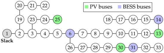
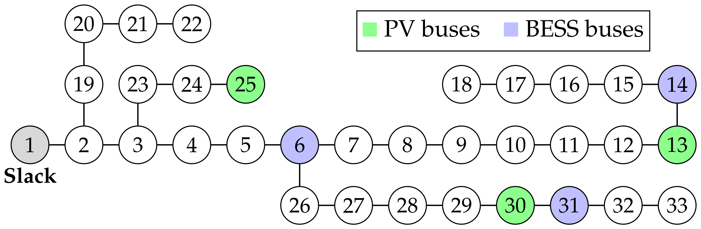
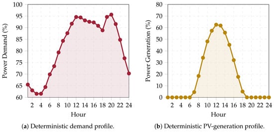
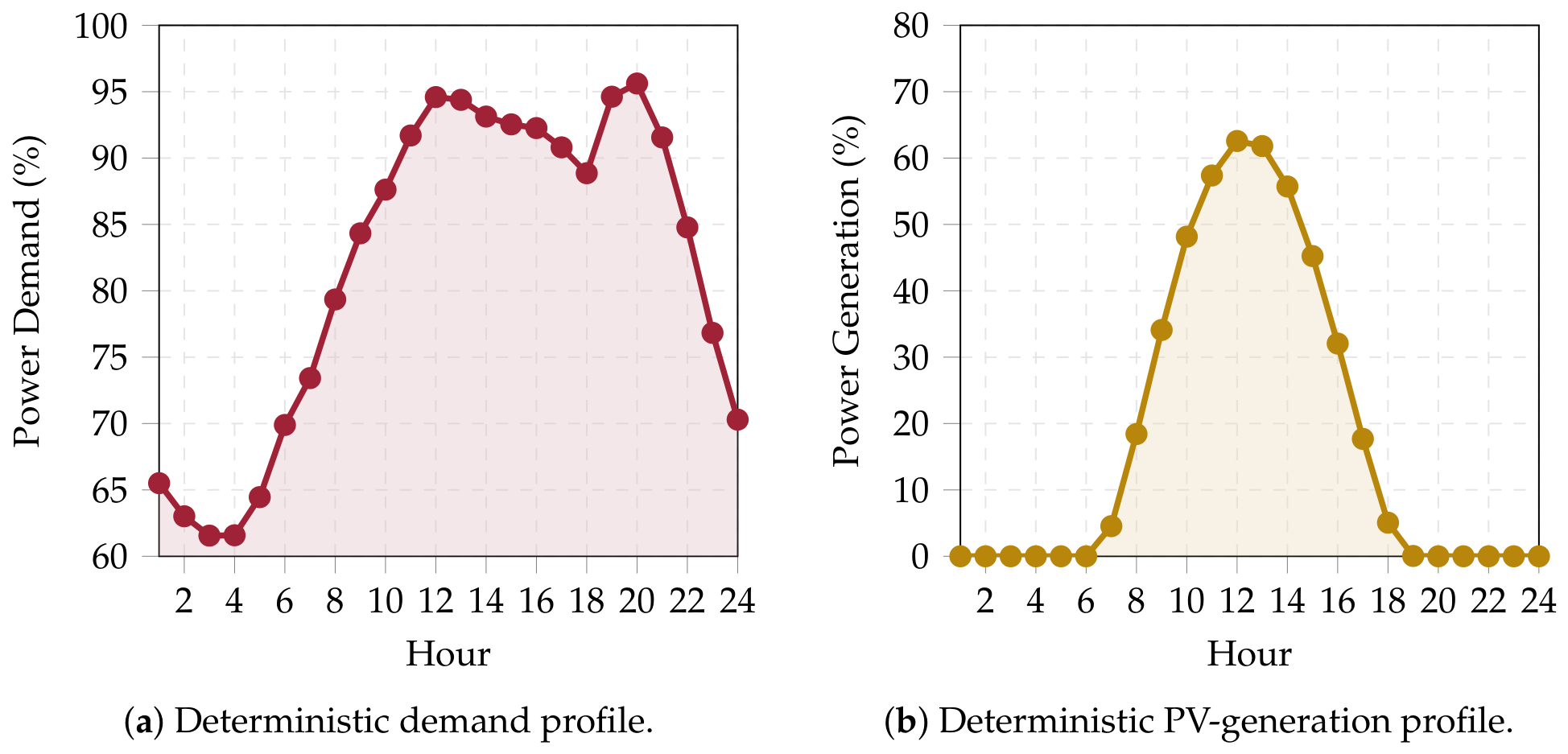
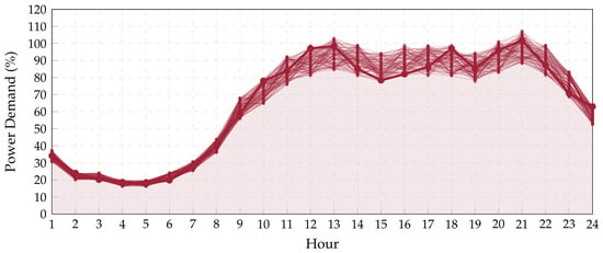
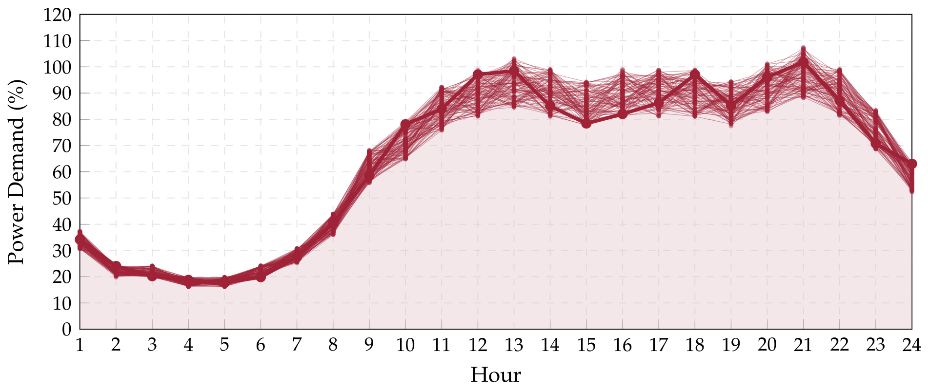
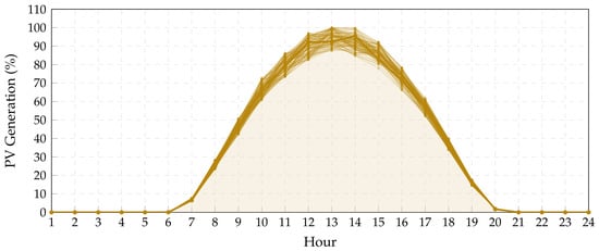
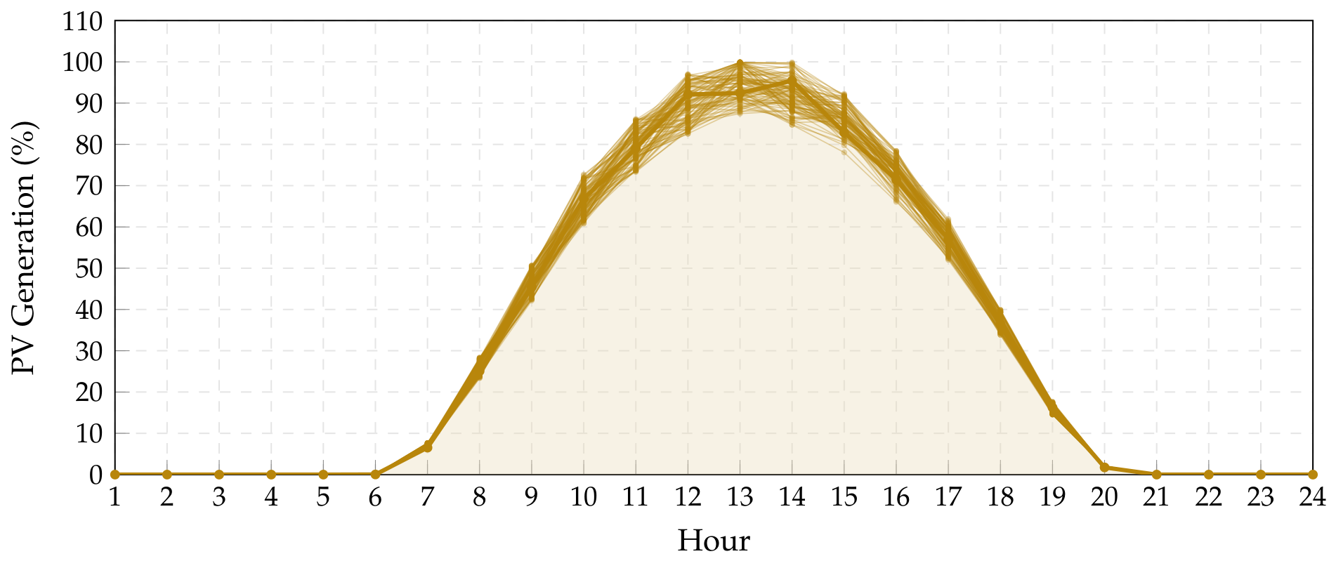
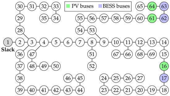
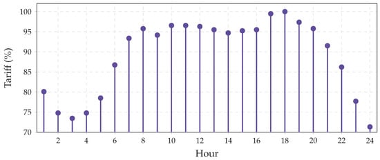
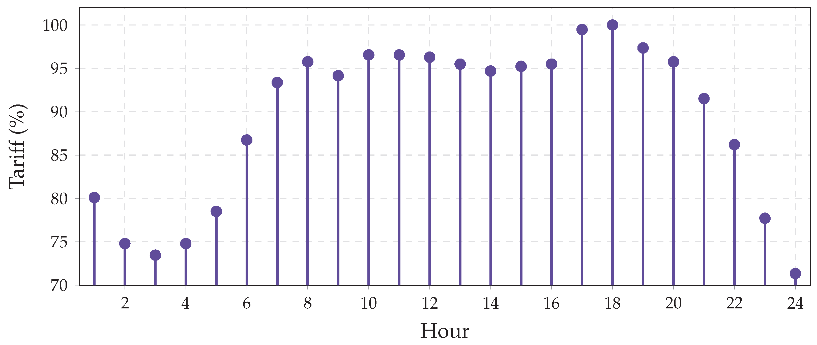
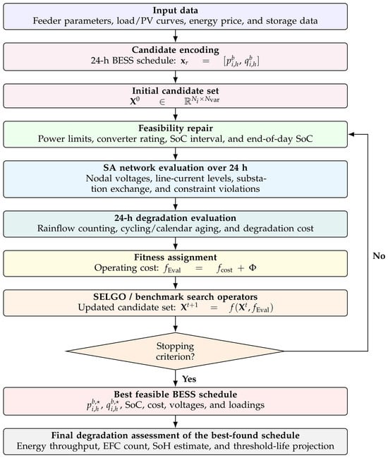
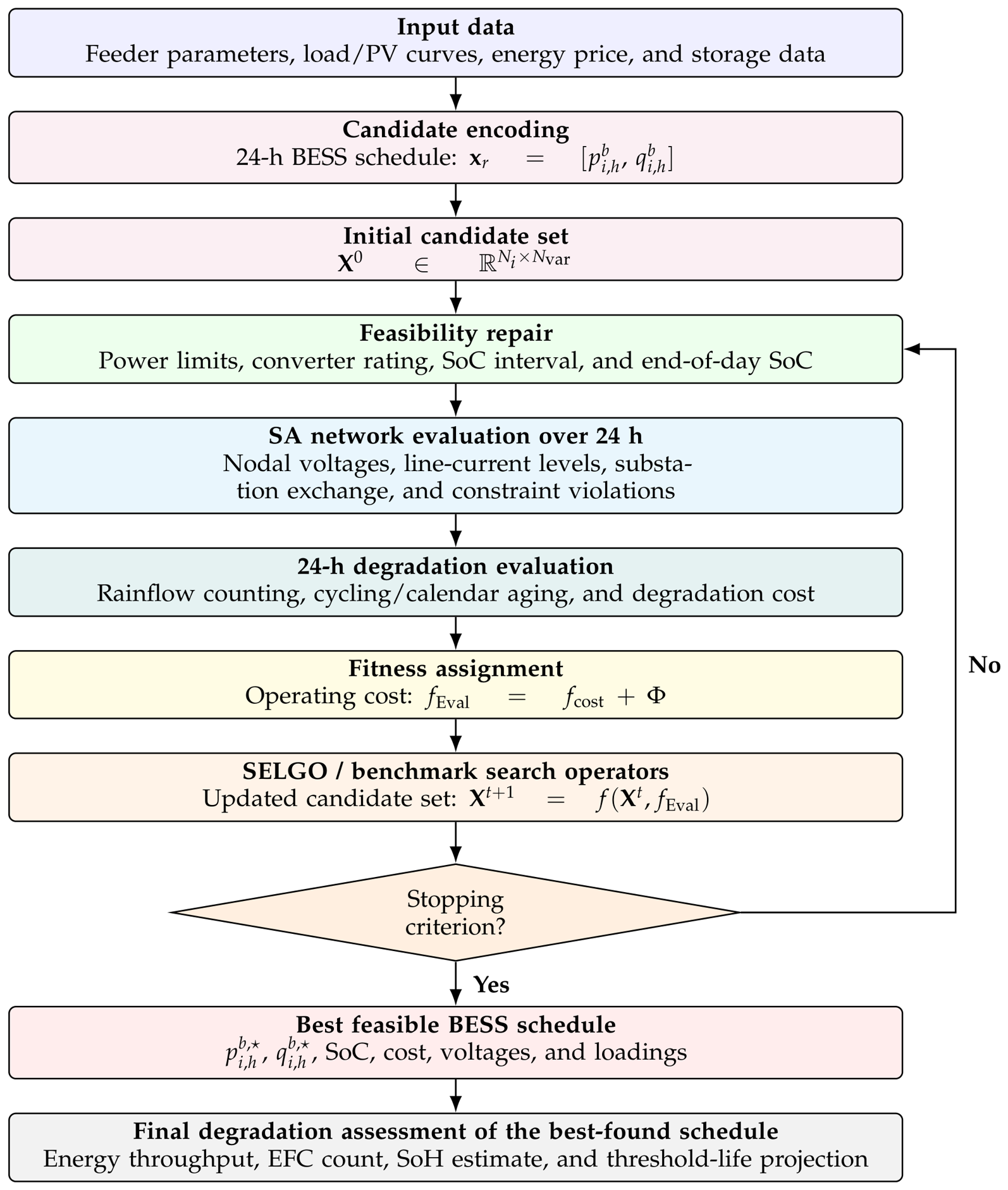
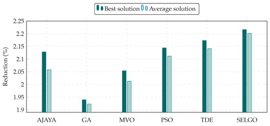
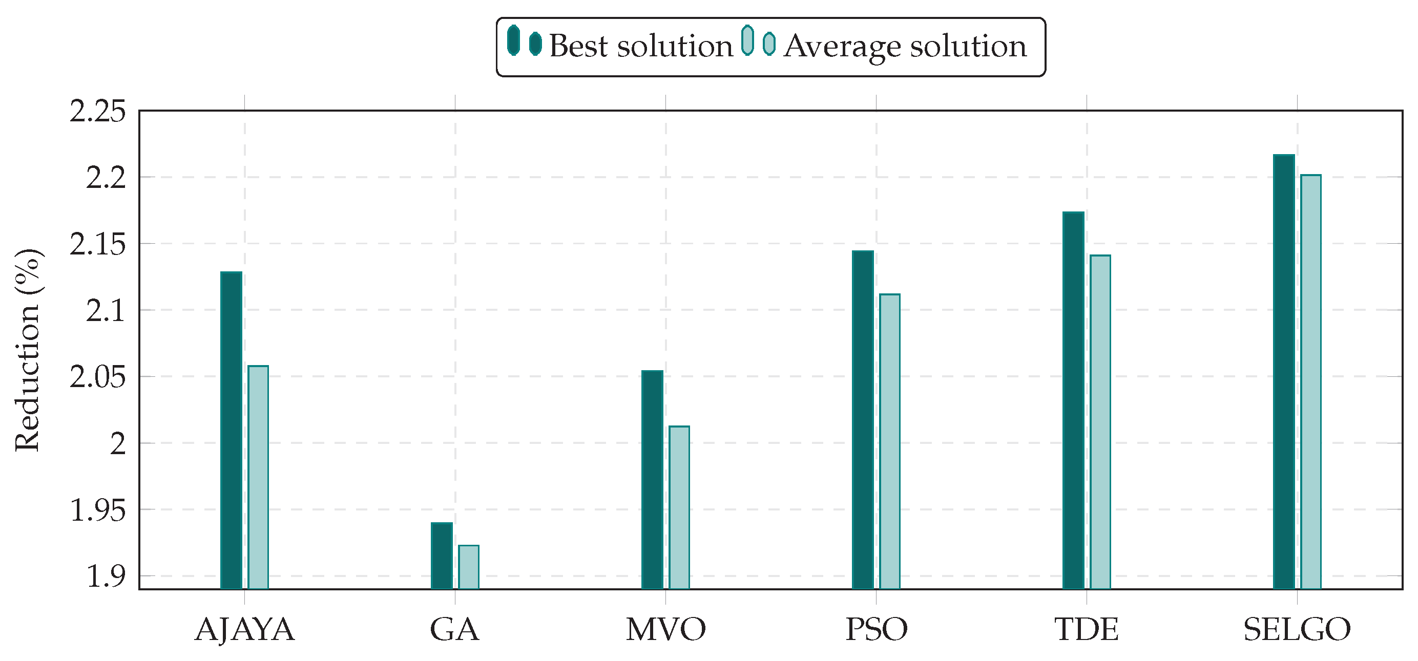
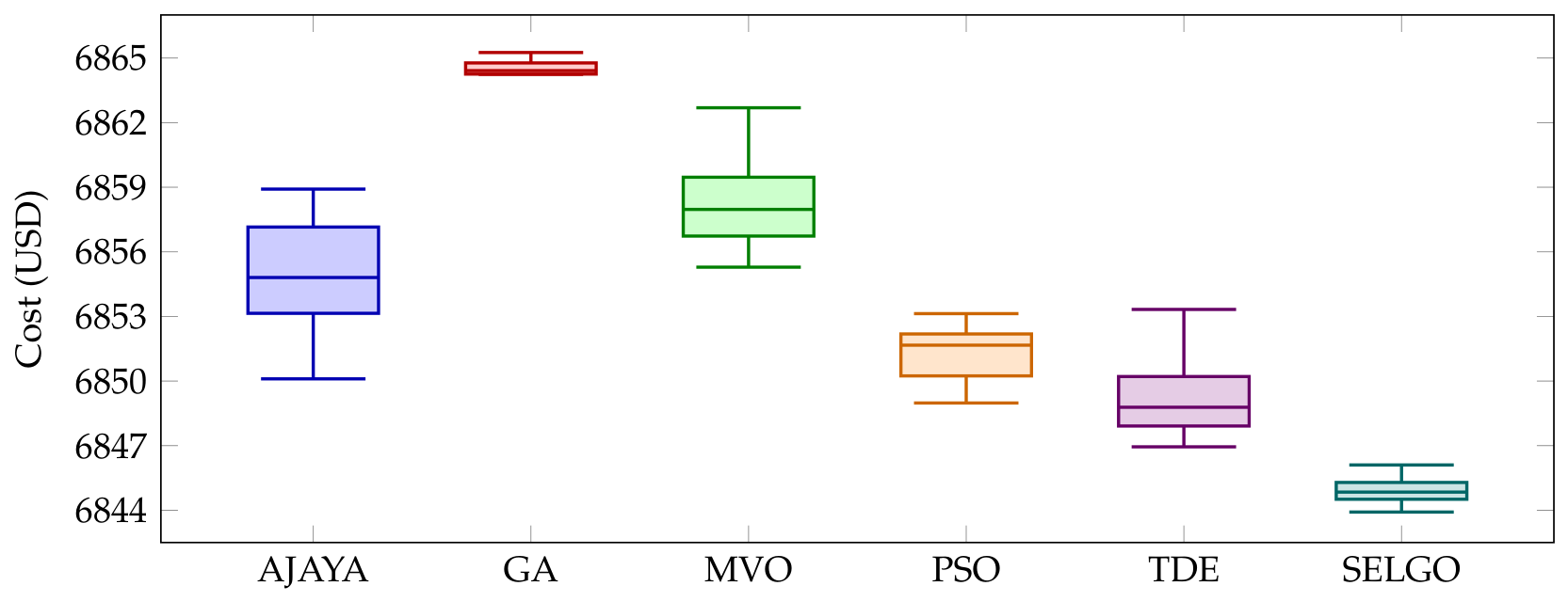
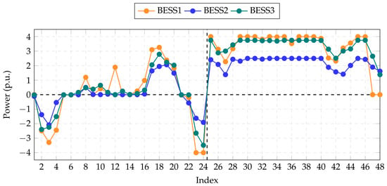
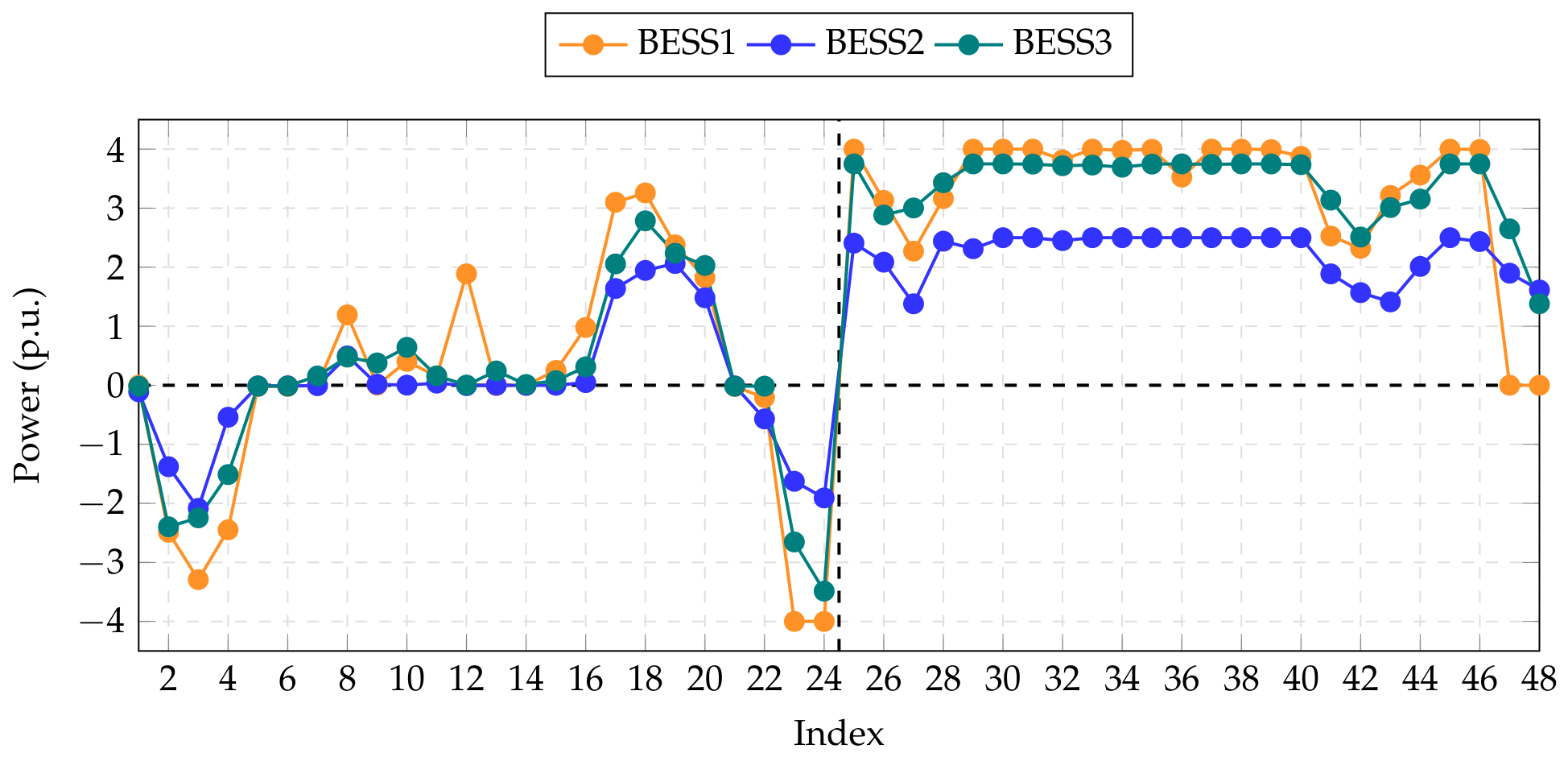
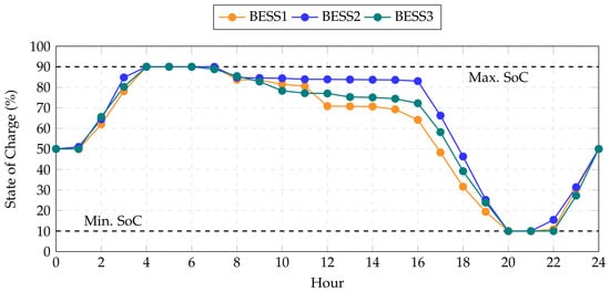
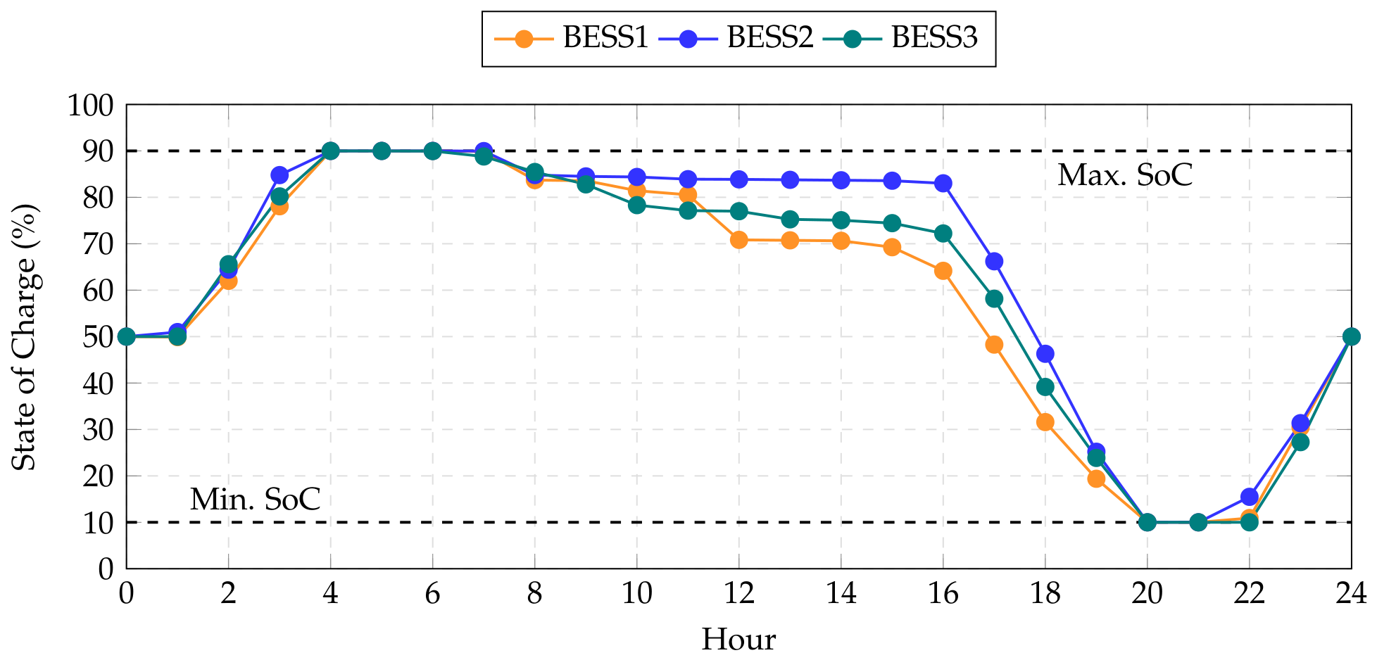
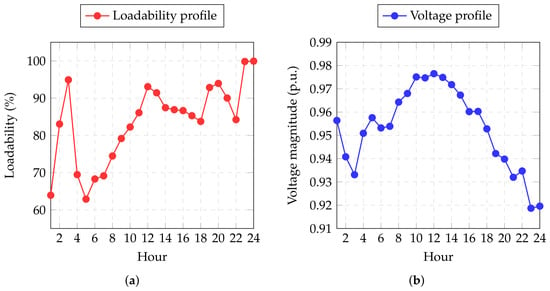
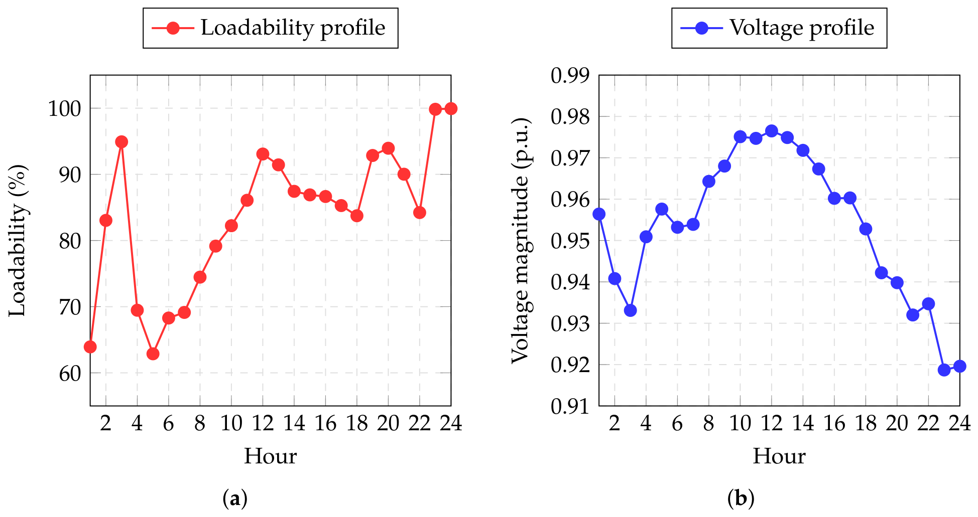
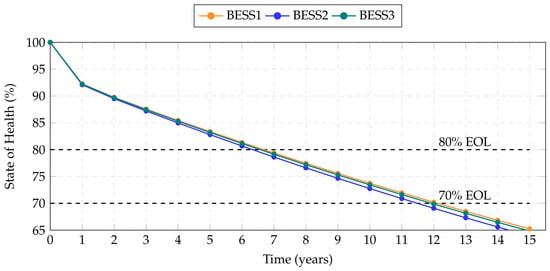
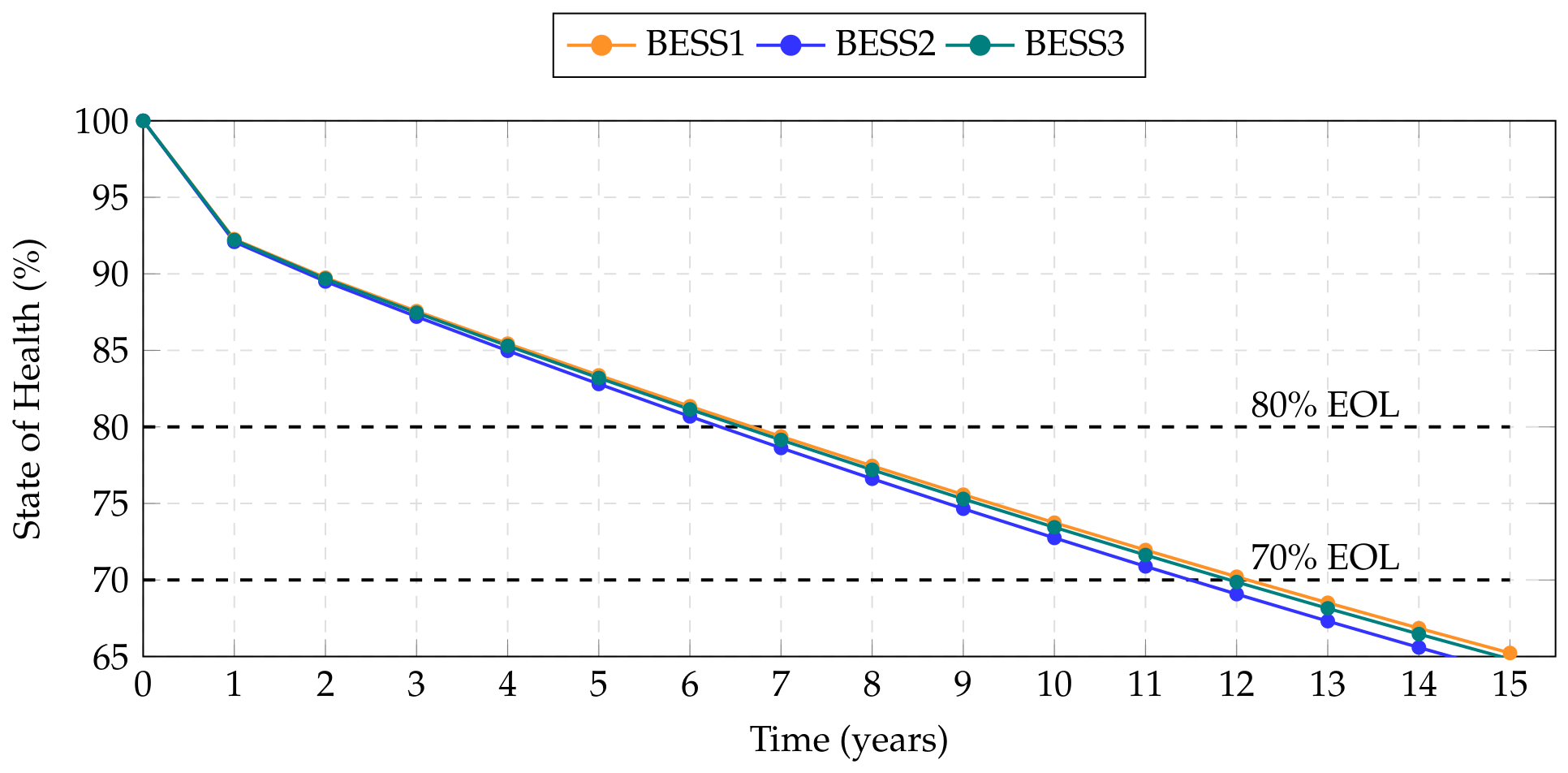
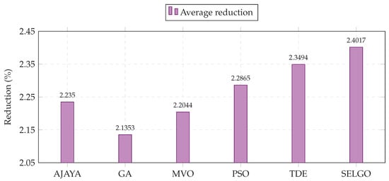
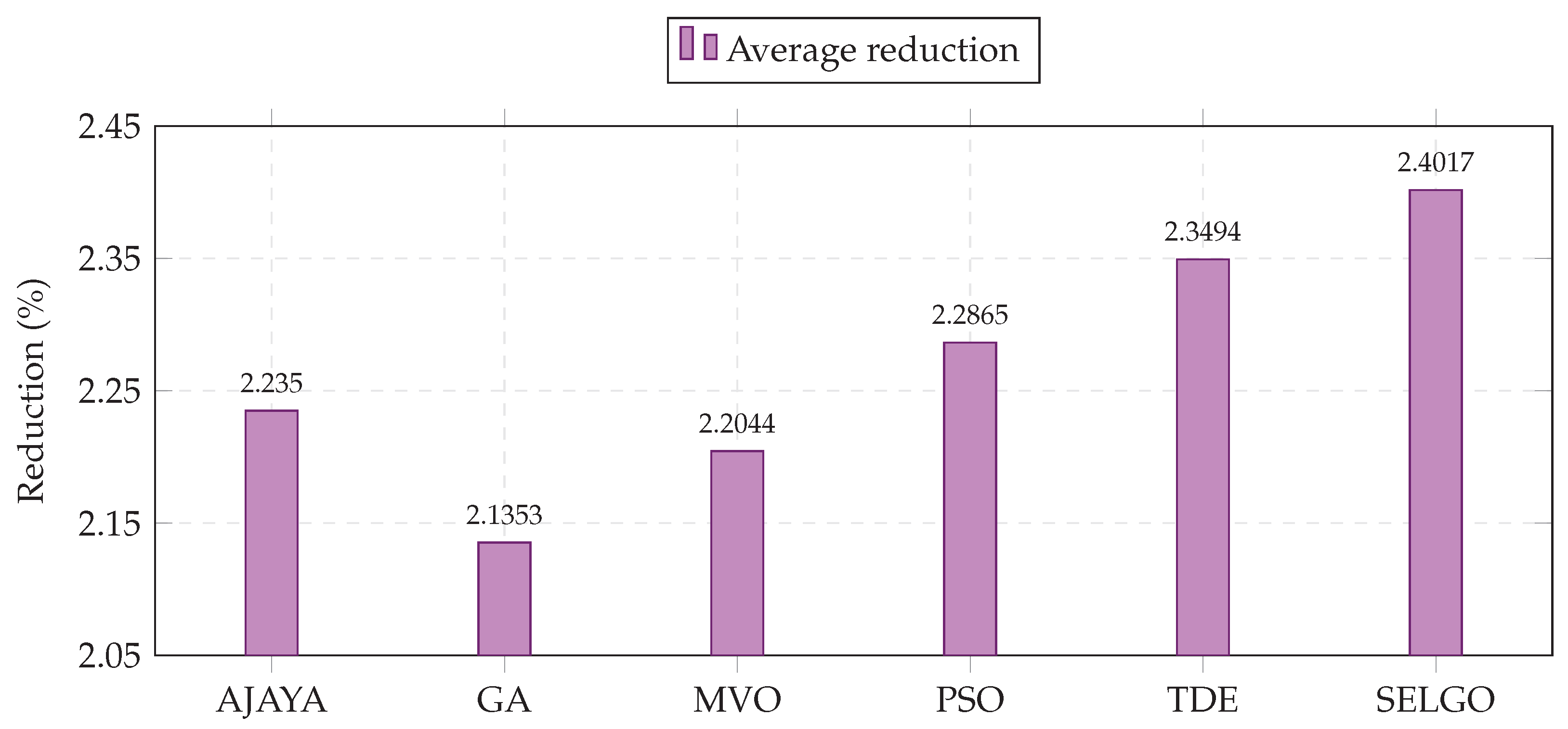
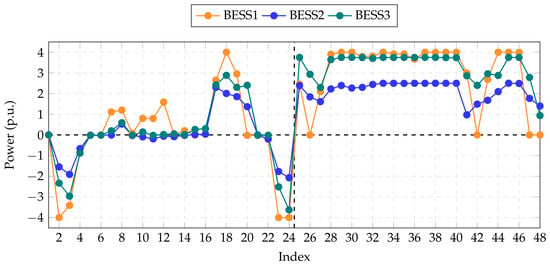
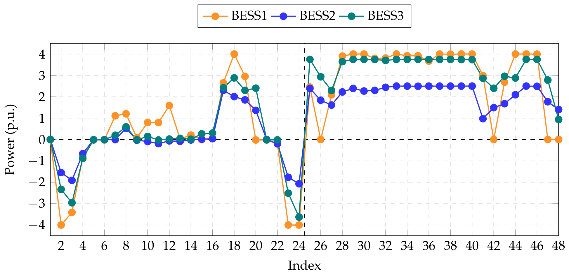
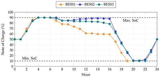
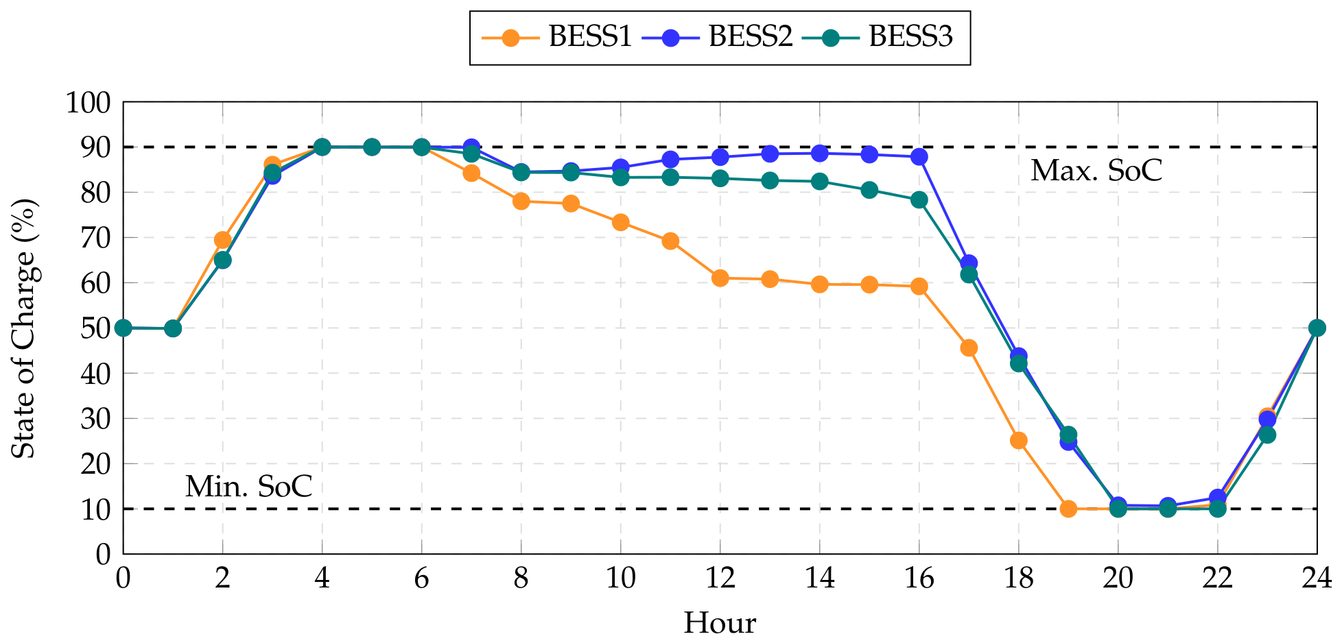
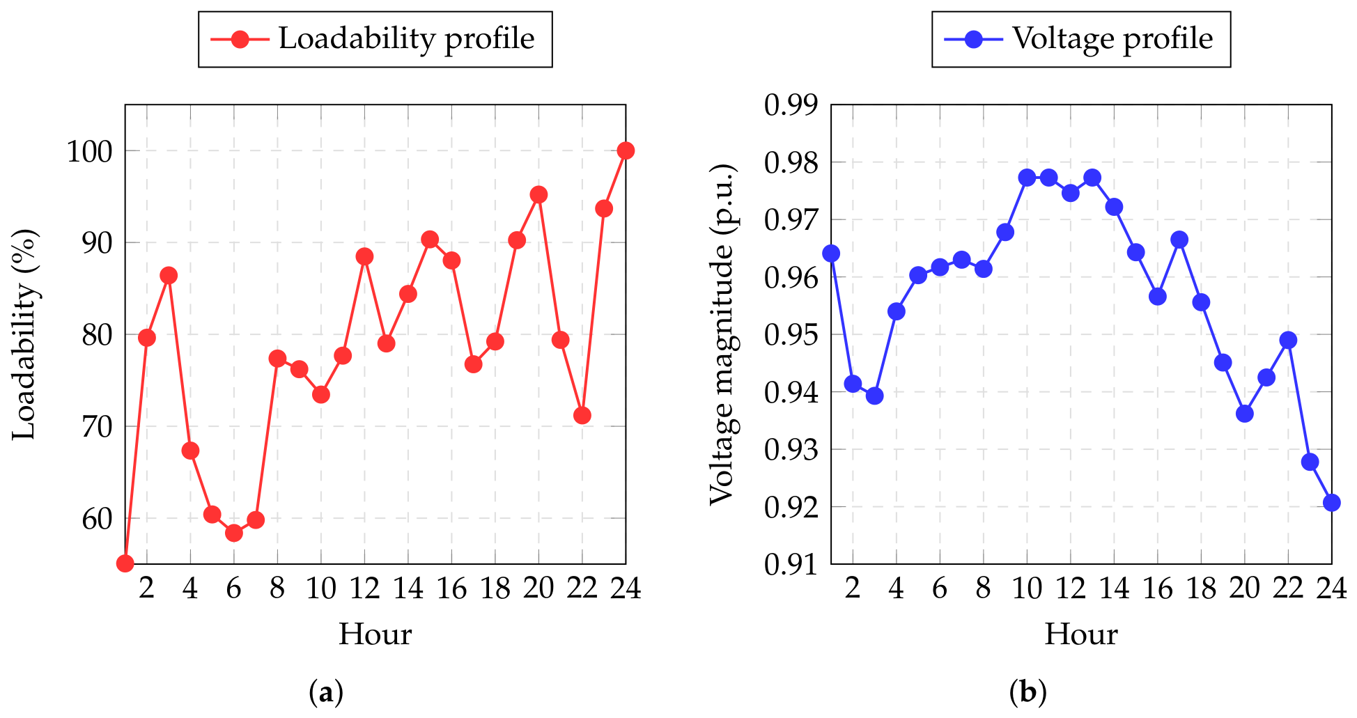
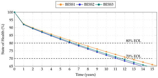
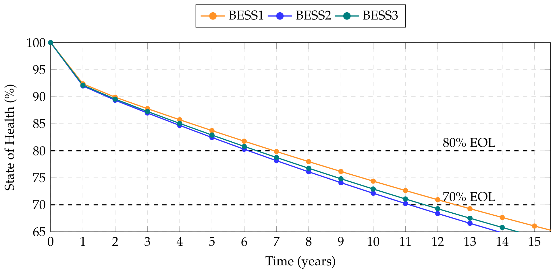
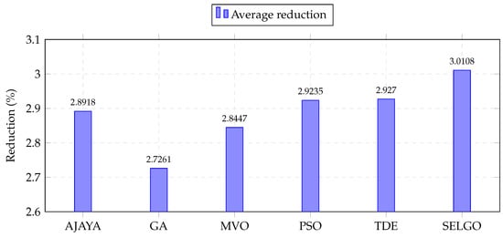
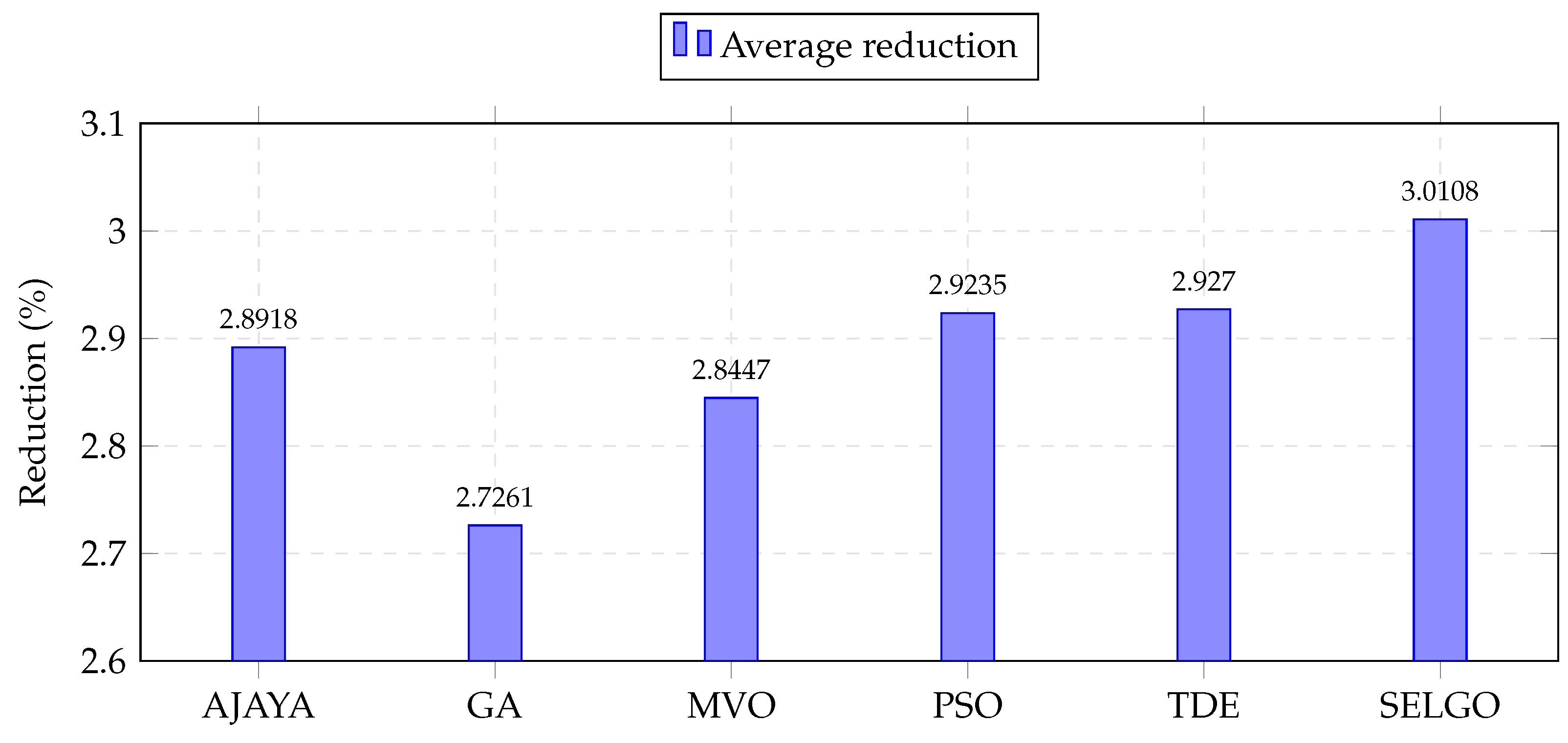
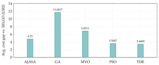
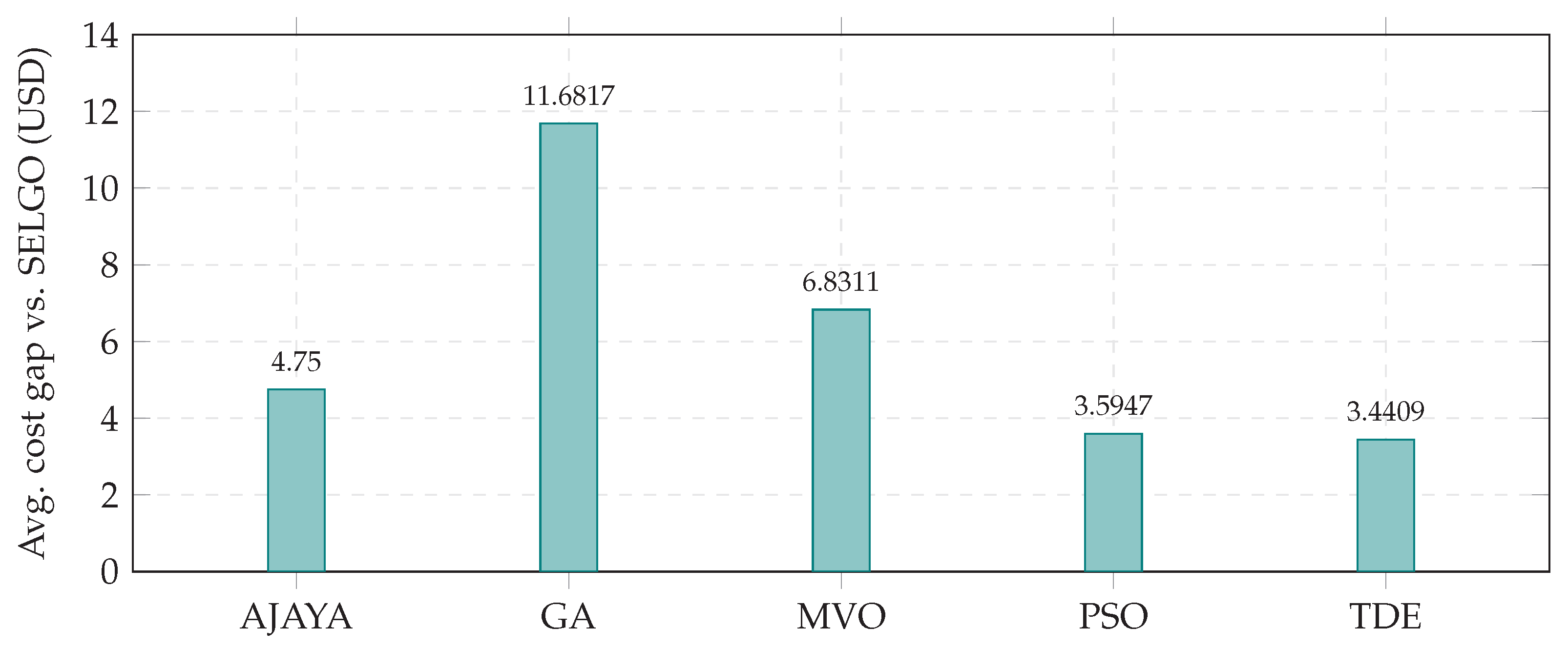
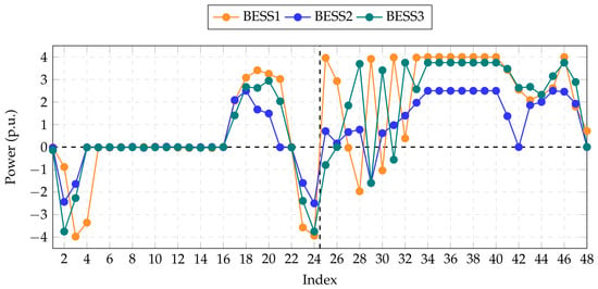
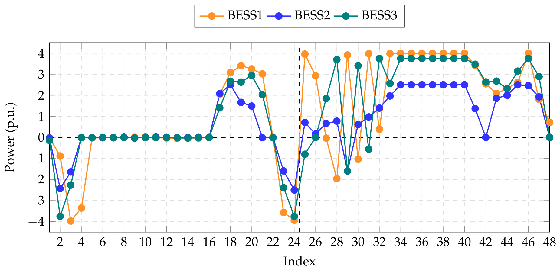
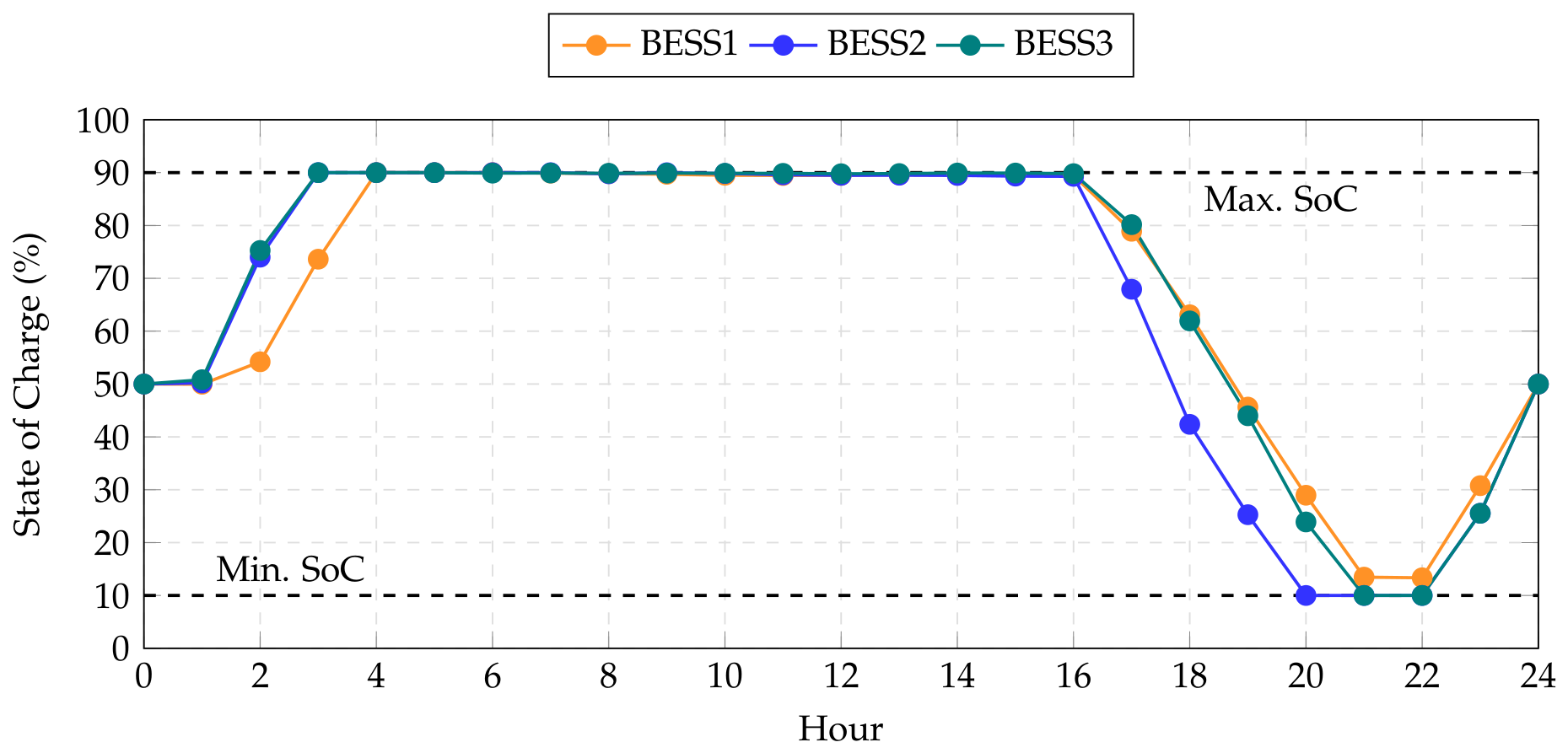
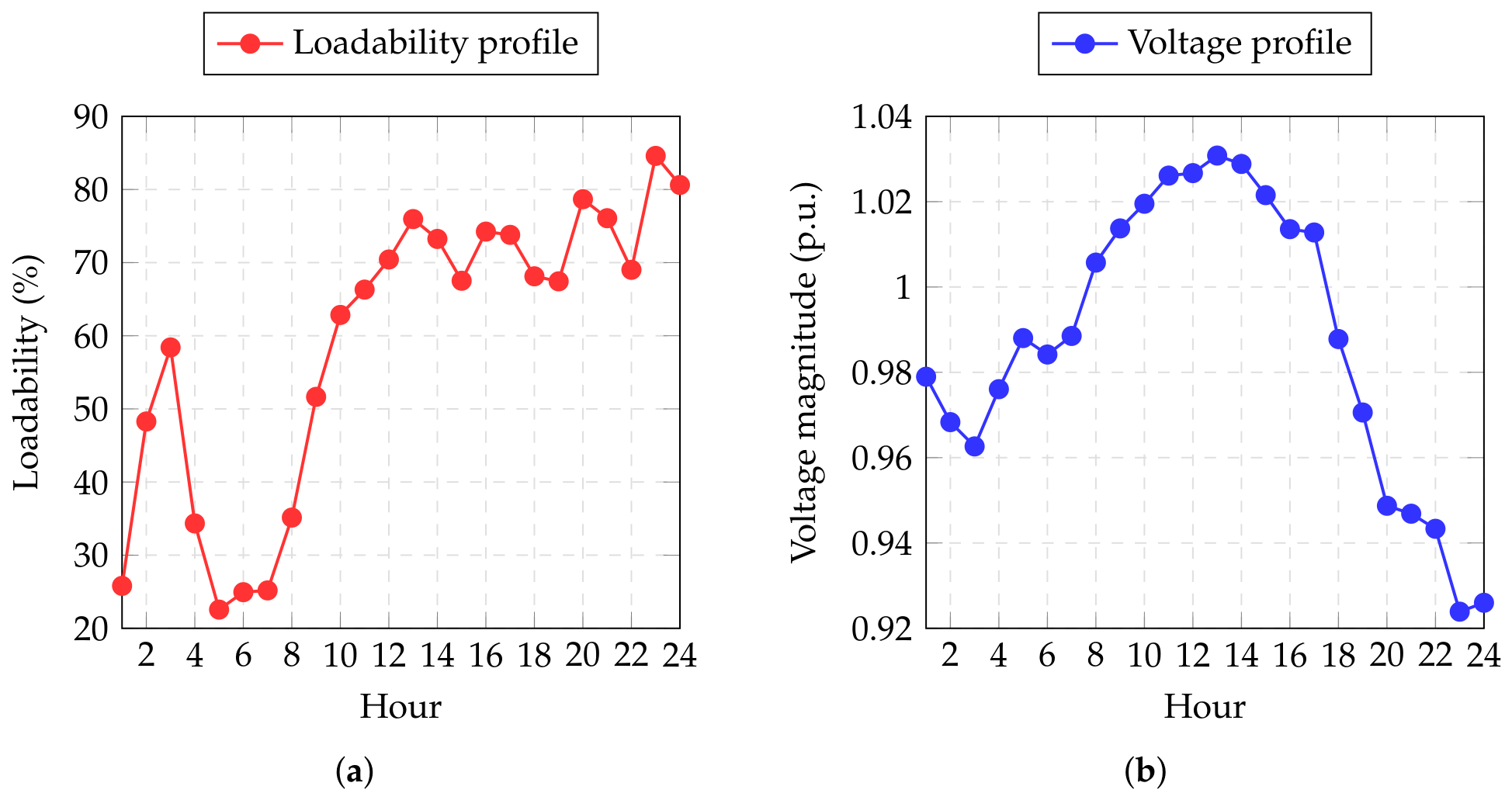
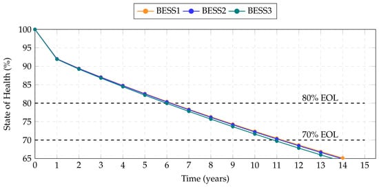
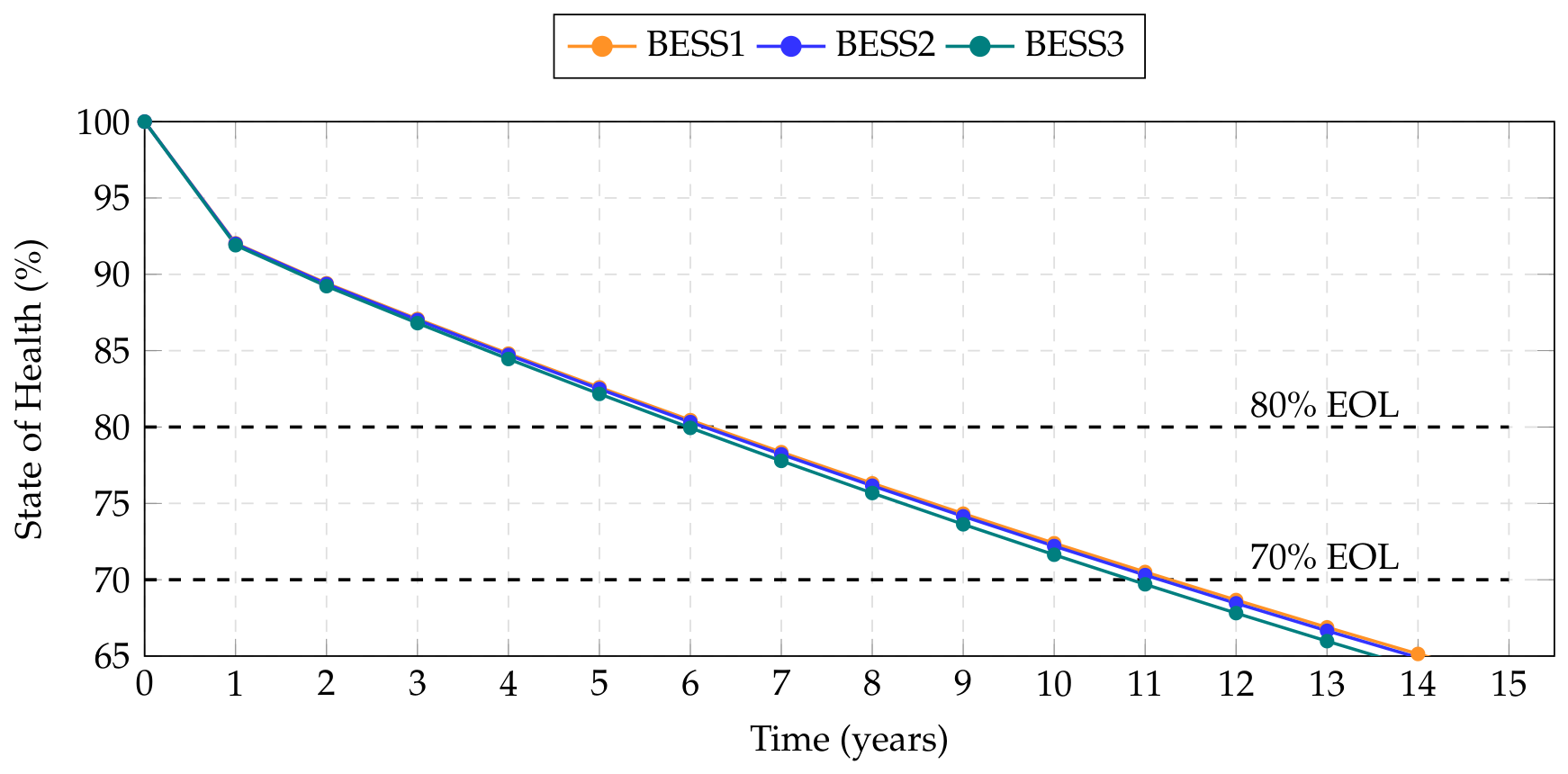
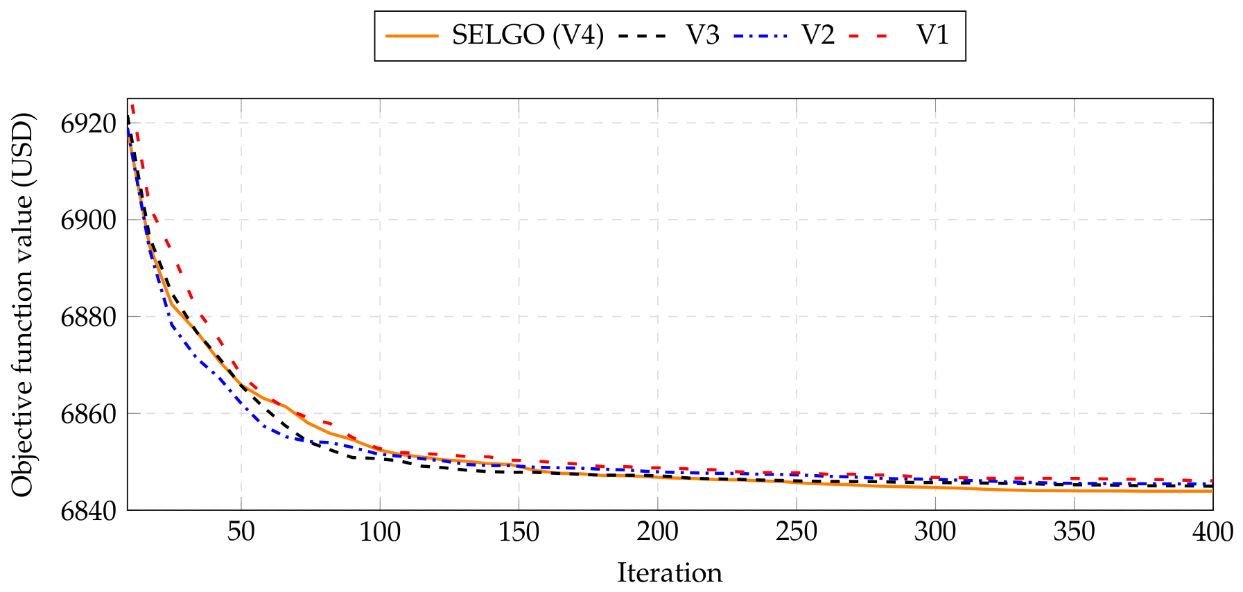
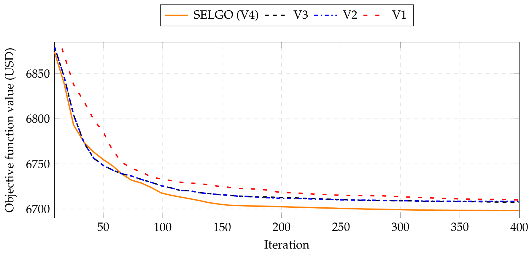
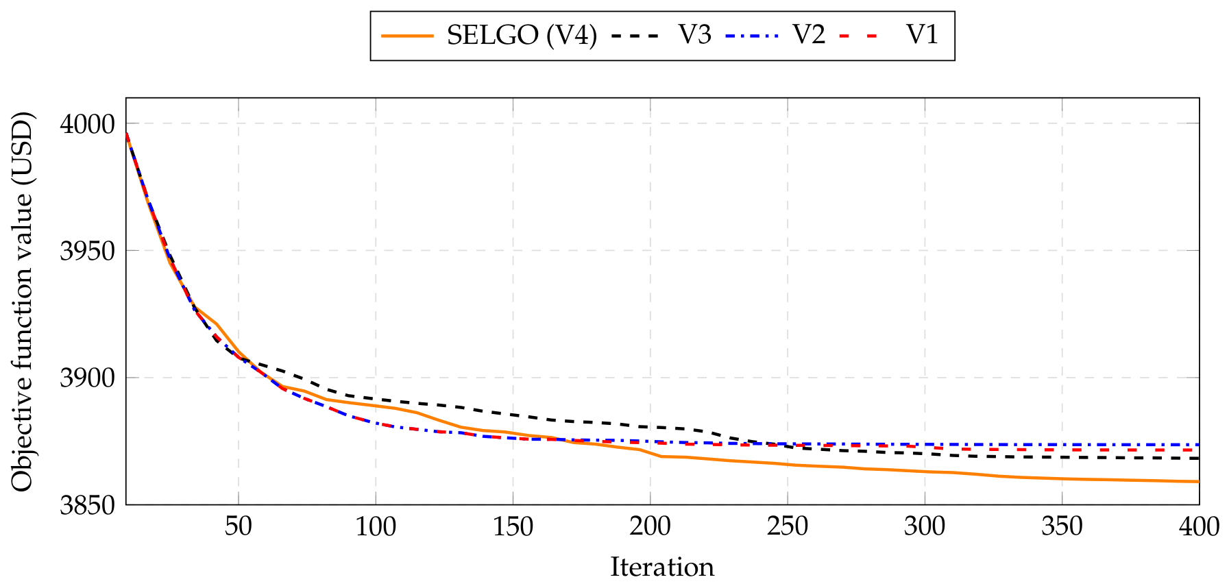
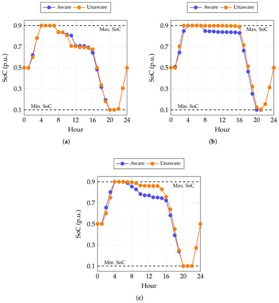
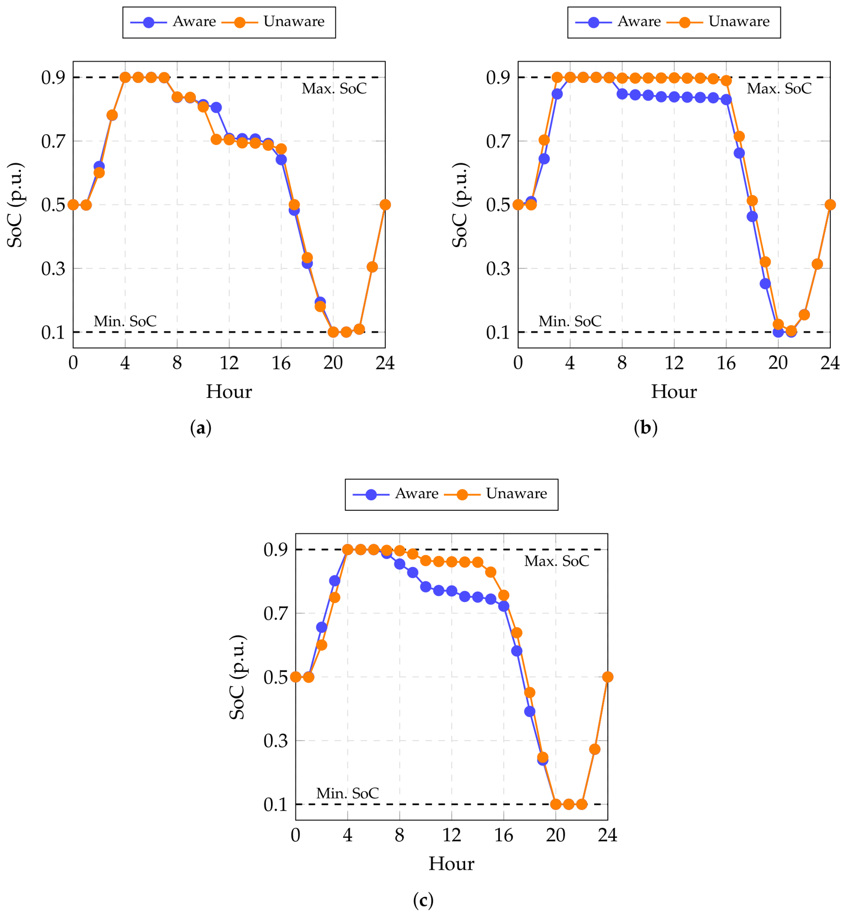

Disclaimer/Publisher’s Note: The statements, opinions and data contained in all publications are solely those of the individual author(s) and contributor(s) and not of MDPI and/or the editor(s). MDPI and/or the editor(s) disclaim responsibility for any injury to people or property resulting from any ideas, methods, instructions or products referred to in the content. |
© 2026 by the authors. Licensee MDPI, Basel, Switzerland. This article is an open access article distributed under the terms and conditions of the Creative Commons Attribution (CC BY) license.