


Abstract
This study examines whether external terms of trade (TOT) maintain a long-run equilibrium relationship with the real GDP of Peru’s construction sector and whether sectoral activity adjusts when deviations from that equilibrium arise. Construction holds substantial economic and social importance in Peru through its close links with investment, employment, infrastructure development, and domestic economic activity. Despite this relevance, empirical evidence on the long-run relationship and adjustment dynamics between external TOT and construction-sector performance remains scarce, particularly for Peru. To address this gap, the study applies Johansen cointegration and a Vector Error Correction Model (VECM) to quarterly data for 2002–2025, incorporating gross fixed capital formation as a control and seasonal effects. Under the selected baseline specification, the results identify one cointegrating relationship, although this evidence is sensitive to the lag-order specification. Construction GDP exhibits a negative and statistically significant error-correction coefficient, with approximately 31% of the preceding disequilibrium corrected within one quarter. In contrast, TOT shows no significant error-correction response, while the weak-exogeneity test supports its role as an external condition within the system. No statistically significant association is identified between lagged TOT changes and construction GDP at the individual short-run lags considered. The findings therefore reveal an asymmetric adjustment process in which construction activity participates in restoring long-run equilibrium while TOT remains weakly exogenous.
1. Introduction
Small open economies are highly exposed to disturbances originating in international markets, whose effects rarely remain confined to activities directly involved in foreign trade [1]. Changes in international prices gradually affect national income, economic agents’ expectations, the resources available for investment and the general conditions under which productive activity takes place [2]. These effects often spread to sectors whose performance depends mainly on domestic economic dynamics. Construction is one of the clearest examples of this interaction [3,4].
In Peru, construction accounts for approximately 6.4% of real GDP and provides employment for nearly 1.16 million people. It is also one of the main destinations of infrastructure investment and capital formation. Over the past 25 years, the sector’s real GDP increased from PEN 9.46 billion to PEN 38.82 billion, reflecting sustained expansion over recent decades [5,6]. Although construction activity takes place mainly within the domestic market, its performance—represented here by real construction-sector GDP—is closely linked to the economic cycle through public and private investment, infrastructure expansion and capital formation [7]. Consequently, the sector tends to respond to prevailing macroeconomic conditions and is particularly sensitive to changes in the international economic environment [8].
As a small open economy with an export structure concentrated in primary commodities, Peru remains exposed to fluctuations in international markets. Their effects extend beyond export-oriented activities and eventually spread to sectors driven by investment and domestic demand [9,10]. In this context, understanding how external conditions become reflected in the performance of domestic sectors is increasingly relevant for both research and public policy. One indicator of these external conditions is the external terms of trade index (hereafter, TOT), defined as the ratio of the export price index to the import price index [11]. Beyond this accounting definition, TOT provides a synthetic indicator of the international economic environment by capturing relative changes in external prices that shape the macroeconomic conditions faced by small open economies such as Peru [12].
Changes in TOT can affect foreign-exchange earnings, fiscal revenues, investment expectations, and overall aggregate demand conditions. Although these effects initially emerge in activities linked to foreign trade, they gradually spread throughout the economy through different macroeconomic mechanisms [13,14]. It is therefore reasonable to expect that construction, whose growth is closely related to investment and overall economic performance, may maintain a systematic relationship with TOT even though it is not strictly an export activity.
The possible relationship between TOT and construction activity does not operate through a single economic mechanism, but through the interaction of several transmission channels. One channel works through public investment, since improvements in TOT tend to increase fiscal revenues associated with export activities, thereby expanding the resources available to finance infrastructure and other investment projects [15]. At the same time, favourable external conditions tend to strengthen business expectations and financing conditions, encouraging private investment in residential, commercial and industrial projects. The sector’s cost structure may also be affected by external conditions because some machinery, specialised equipment and other inputs used in construction depend directly or indirectly on international markets [16,17]. Taken together, these mechanisms suggest that persistent fluctuations in TOT may ultimately be reflected in the economic trajectory of the construction sector.
Despite the economic plausibility of these mechanisms, empirical evidence specifically examining the relationship between TOT and real construction-sector GDP remains relatively limited. Internationally, several studies have analysed construction activity from a macroeconomic perspective, relating it to variables such as investment, economic growth, business cycles, financial conditions and international trade [18,19]. Other studies show that external shocks may spread to economic activity through changes in public investment, credit availability or business expectations, particularly in emerging economies that depend on natural-resource exports [20,21,22]. Nevertheless, differences in approaches, variables, and institutional settings make it difficult to draw general conclusions about the long-run relationship between TOT and the economic performance of the construction sector.
This limitation is even more apparent in Peru. The available literature has focused mainly on the effects of TOT on aggregate variables such as gross domestic product, consumption, investment, the exchange rate, the trade balance, and fiscal accounts [23,24,25]. Although these studies have contributed to understanding the role of external conditions in the country’s macroeconomic performance, no research has been identified for Peru that directly examines the long-run relationship between TOT and real construction-sector GDP. This is precisely the gap addressed by the present study.
From this perspective, the study considers the possibility that mechanisms such as public investment, private investment, business expectations, and imported-input costs, through which external conditions may be transmitted to construction activity, could contribute to the long-run association between TOT and real construction-sector GDP. However, the econometric framework does not separately identify these transmission channels or quantify the dynamic response of construction output to TOT innovations. This approach is consistent with the nature of small open economies, where external disturbances may operate through several channels whose individual influence is difficult to isolate empirically.
Against this background, the objective of this study is to examine whether TOT maintains a long-run equilibrium relationship with real construction-sector GDP in Peru and to determine whether the sector adjusts its trajectory when deviations from that equilibrium occur. The existence of such a relationship would be consistent with the idea that sectoral performance remains systematically associated with the external macroeconomic environment. For this purpose, the study adopts a time-series approach based on Johansen’s cointegration methodology and a Vector Error Correction Model (VECM), using quarterly data for 2002–2025. This framework makes it possible to identify long-run equilibrium relationships among integrated variables and to analyse how temporary disequilibria are corrected over time. It therefore allows us to establish not only whether a persistent association exists between TOT and real construction-sector GDP, but also which variables systematically adjust when deviations from long-run equilibrium occur.
The main contribution of this research is to extend the empirical evidence on the relationship between TOT and sectoral economic performance from a long-run perspective by bringing construction into an area of research that remains scarcely explored in Peru. The study also provides evidence for understanding the long-run association between external conditions and the performance of an activity closely connected with investment, capital accumulation, and infrastructure development. In doing so, it offers useful insights into the long-run macroeconomic relationships relevant to construction-sector performance in economies exposed to persistent fluctuations in the international environment.
1.1. Literature Review
1.1.1. Terms of Trade, Economic Performance and Construction-Sector Dynamics
Empirical evidence on the relationship between TOT and economic performance shows heterogeneous results across countries and productive structures. Studies conducted in the United States and Bangladesh identified long-run relationships between TOT and economic growth, although with negative associations in both the short and long run [26,27]. By contrast, research covering economies with different levels of development and openness shows that favourable effects tend to be concentrated in low- and middle-income countries with better export conditions, while poorer economies do not necessarily benefit from a favourable external environment [28].
This heterogeneity becomes more apparent when the productive and trade composition of economies is considered. Evidence from the United States and China shows that the effect of TOT on growth differs across food, fuels, goods, and information and communication products [29,30], while an analysis of 178 countries documented asymmetric responses between commodity-exporting and commodity-importing economies [31]. Taken together, these findings indicate that external conditions are not transmitted through a uniform mechanism, but depend on each economy’s trade structure and degree of international exposure.
The literature also shows that the nature of commodities and prevailing macroeconomic conditions shape how economies respond to TOT. Positive, negative, and even weakly significant effects of external shocks have been identified in developing and emerging economies, with metal-related shocks showing a stronger influence [20]. Similarly, in net commodity-exporting countries, the relationship between commodity prices and growth varies according to inflation levels and the type of commodity [32]. Other studies report favourable effects during commodity booms, although responses to positive and negative shocks are asymmetric [33]. Commodity TOT growth has also been found to favour real output per capita, while its volatility may constrain growth by reducing the accumulation of physical and human capital [34].
The effects of external conditions are not confined to aggregate economic performance and may also differ across sectors. In emerging markets, different sectoral sensitivities to international macroeconomic determinants have been identified [35], while a study covering 46 African countries showed that several structural changes in real GDP per capita coincided with TOT shocks associated with large fluctuations in primary commodity prices [36]. Similarly, cointegration techniques were used in India to examine the long-run relationship between TOT and both public and private agricultural investment, indicating that an improvement in TOT favours investment and, through this channel, the sector’s productive performance [37]. Taken as a whole, this evidence suggests that external conditions may spread differently across sectors, mainly through investment and capital accumulation processes.
This perspective is particularly relevant to construction, whose interaction with the macroeconomic environment has been documented in many countries. International evidence shows that the relationship between construction activity and economic development is complex [38] and that its relative importance changes as the development process advances, as observed in Asian and Latin American countries, including China, Mexico and Argentina [39]. In Cape Verde, construction was found to follow the general trajectory of the economy during periods of economic expansion [40], while evidence from Ecuador and Indonesia identified a positive association between aggregate GDP growth and construction-sector performance [41,42].
Nevertheless, the relationship between construction and economic activity does not follow a uniform pattern either. In Poland and 26 other European Union countries, different lags were identified between GDP growth and indicators of construction activity [43]. Similarly, research covering Türkiye and ten European Union countries documented long-run relationships among construction, GDP, investment, foreign direct investment, taxation and interest rates [44]. Studies conducted in Hong Kong, India and China also show that the interaction between construction and growth may involve bidirectional causal relationships, unidirectional effects or persistent links with long-term investment [19,45,46]. Overall, these results show that the sector’s response depends on the economic and institutional characteristics of each country.
The sensitivity of construction to the macroeconomic environment has also been documented from other perspectives. The literature relates its performance to variables such as output, fiscal policies, investment, savings, the balance of payments, interest rates and prices [47]. In Türkiye, the cyclical nature of the sector and its sensitivity to GDP, money supply and input costs have also been highlighted [48]. In China, an analysis of 30 provinces found heterogeneous relationships among financial development, construction and GDP [49], while evidence from countries in the Americas, Asia and Europe shows that the influence of inflation and interest rates on construction differs across economies [44]. These findings reinforce the idea that sectoral performance responds to a broad set of macroeconomic conditions whose importance varies according to the context examined.
Other studies provide further evidence in this direction. In India, the relationship between construction and growth was found to depend on the inclusion of capital stock and employment [50], while in Malaysia cointegrating relationships were identified between construction and sectors such as agriculture, manufacturing, services and mining [51]. In Nigeria, different studies found that aggregate output precedes construction performance in both the short and long run, that a bidirectional relationship exists between them, and that bank credit is closely associated with the sector’s evolution [8,52,53]. Taken together, these results show that the trajectory of construction is closely associated with the conditions supporting investment, financing and overall economic activity.
The influence of external conditions becomes particularly important in small open economies. In Northern Cyprus, a long-run equilibrium relationship was identified among construction value added, real GDP, money supply and foreign capital transfers [54]. Similarly, in Trinidad and Tobago, an economy dependent on oil and gas, positive relationships were found between hydrocarbon revenues and prices and construction value added. The sector was also found to grow more strongly during expansionary periods and to contract more rapidly during recessions [55,56]. Overall, these findings support the possibility that disturbances originating in activities closely connected with international markets may ultimately be reflected in the performance of a predominantly domestic sector such as construction.
The sector’s external exposure may also operate through input markets and supply chains. In the United States, construction materials were found to depend heavily on imported commodities, while changes in import quantities may be transmitted asymmetrically to the prices of different materials [57]. Research conducted in Singapore and the United States also shows that construction has strong interdependencies with other sectors of the economy and that its performance is related to GDP and construction expenditure [58,59]. Consequently, the sector’s sensitivity to the economic environment depends not only on its direct participation in foreign trade, but also on its integration with investment, credit, input markets and the multiple productive interrelationships that characterise its activity.
Finally, the evidence reviewed indicates that the relationship between TOT and economic performance is heterogeneous and may therefore display different characteristics at the sectoral level. Construction, in turn, responds to various macroeconomic conditions, including some originating in the external environment. However, these two areas of research have developed largely along separate lines. To the extent covered by the literature reviewed, no studies have been identified that directly examine whether TOT and construction-sector GDP maintain a long-run equilibrium relationship or how adjustment occurs following deviations from that equilibrium. This gap is particularly relevant for a small open economy such as Peru, where external conditions may spread to predominantly domestic activities through investment, income, financing, and input costs. In this direction, it is necessary to review the time-series evidence and econometric approaches used to identify long-run relationships and adjustment mechanisms in comparable settings.
1.1.2. Time-Series Evidence and Long-Run Relationships
From a methodological perspective, a substantial body of research has used time-series techniques, cointegration, and error-correction models to examine the persistence of relationships between external conditions and economic performance. In the United States, Bangladesh, and China, long-run relationships between TOT and economic growth were identified, together with adjustment mechanisms that correct deviations from equilibrium [26,27,29]. These methods have also been extended to sectoral analysis. In emerging markets, a VECM was used to identify different sectoral sensitivities to international macroeconomic determinants [35], while Engle-Granger and Johansen-Juselius procedures were applied in India to study the relationship between TOT and agricultural investment [37]. Similarly, studies conducted in Türkiye, Poland and other European Union countries, Cape Verde, Malaysia, China, Northern Cyprus and Nigeria used cointegration, causality, ARDL and VECM approaches to analyse the relationship between construction, GDP and other macroeconomic variables [8,40,43,44,49,51,52,53,54].
In the Peruvian case, these approaches have also been used to examine long-run relationships between TOT and different macroeconomic and sectoral variables. Available studies identify cointegrating relationships between exports and aggregate GDP, as well as between TOT and national GDP, confirming that external conditions form part of the long-run dynamics of the Peruvian economy [60,61]. Similarly, studies of the mining and agricultural sectors applied the Johansen cointegration approach and VECM models to identify long-run equilibrium relationships. Their findings show that adjustment to disequilibria occurs mainly through sectoral GDP, while TOT behaves as a weakly exogenous variable [62,63]. However, no studies have been identified that examine this relationship specifically for the construction sector, and even fewer that address it using a cointegration and VECM framework. This gap is relevant because it limits our understanding of how external conditions are associated with an activity whose evolution is closely linked to the macroeconomic environment, thereby providing the rationale for the methodological approach adopted in the present study.
1.2. Theoretical Framework
The terms of trade index (TOT) is one of the main channels through which international economic conditions become incorporated into the functioning of economies. Besides expressing the relationship between export and import prices, it reflects an economy’s capacity to obtain goods and services from the rest of the world on the basis of the income generated by its exports [11,14]. Changes in TOT therefore represent shifts in the relative prices of foreign trade, as well as changes in the conditions under which countries interact with international markets and, consequently, in the macroeconomic environment that influences production, consumption and investment decisions [64,65].
Its importance becomes even more evident in economies whose international integration depends on a limited number of export products. In these cases, fluctuations in external prices tend to translate into persistent changes in national income, foreign-exchange availability, financing capacity and the expectations of economic agents, gradually altering the aggregate behaviour of the economy [14]. Even when these effects originate outside the domestic market, they rarely remain confined to activities directly associated with the country’s foreign trade [3,66]. Instead, they tend to spread throughout the productive system through a chain of adjustments that affects both investment decisions and the general conditions under which economic activity takes place [67].
From this perspective, TOT can be understood as an external macroeconomic condition whose influence extends beyond the export sector and becomes incorporated, with varying intensity and through different mechanisms, into the performance of activities mainly oriented towards the domestic market. The magnitude of this transmission depends on the structural characteristics of each economy and, of course, on the extent to which its different sectors are connected with macroeconomic variables that respond to developments in the international environment. Consequently, although construction does not participate directly in foreign trade because it is a non-tradable activity, its long-run trajectory may still remain associated with external conditions, as reflected by TOT.
The possible connections between TOT and construction activity do not arise from a single economic mechanism. Rather, they result from the interaction of several processes through which external conditions become incorporated into the domestic economy [13]. One of the most important is related to export income. For example, when the international prices of the products exported by a country improve, the income generated by activities oriented towards foreign trade increases and, at the same time, more resources become available to support aggregate expenditure [14].
In economies where exports of raw materials or natural resources represent a major source of fiscal revenue, this process often translates into greater capacity to finance infrastructure projects. This can expand public investment and stimulate demand for construction-related activities [68,69]. At the same time, when external conditions are favourable, business expectations and financing conditions tend to improve. This usually favours the implementation of residential, commercial and industrial projects, thereby encouraging private investment [70].
However, limiting the transmission of TOT only to income dynamics could provide an incomplete view of the issue, since construction also depends on capital goods and inputs whose availability and cost are linked to international markets. Heavy machinery, specialised equipment, metal components, fuels and other inputs contain, to varying degrees, imported content and externally determined prices [71]. As a result, changes in the international trade environment may also modify the cost structures faced by construction firms, affecting the expected profitability of projects and, consequently, investment and production decisions. This channel operates mainly from the supply side, by affecting construction costs and the economic viability of new investments, which distinguishes it from the income-related mechanism [72].
The presence of both mechanisms in economic activity suggests a possible relationship between TOT and construction-sector performance. This relationship does not depend solely on developments in foreign trade or on the sector’s direct participation in the country’s exports. Rather, it reflects the combined effect of changes that simultaneously influence demand conditions, investment decisions and the cost structure of construction activity [73]. These mechanisms are presented as theoretically plausible transmission channels rather than as channels separately identified by the empirical model. It is therefore reasonable to expect persistent disturbances in TOT to be reflected in the sector’s long-run trajectory, even when the different transmission channels cannot be observed or identified separately within an aggregate econometric model.
From an econometric perspective, the existence of transmission mechanisms that operate persistently raises the possibility that external conditions and construction-sector performance do not evolve independently in the long run. If the effects associated with TOT are systematically incorporated into construction dynamics, both variables may be expected to follow trajectories that are compatible with an equilibrium relationship, even though temporary disturbances may generate deviations in the short run. In this context, cointegration analysis provides an appropriate framework for assessing whether these variables maintain a long-run equilibrium relationship and whether the disequilibria that may arise tend to be gradually corrected [74]. The VECM also allows short-run interactions among the variables to be examined empirically, without presupposing that the theoretical transmission mechanisms described above must generate statistically significant short-run effects.
2. Materials and Methods
2.1. Research Design, Data and Variables
In this study, we adopted a quantitative, applied approach with an ex post facto design and a time-series framework, since the analysis relies on previously observed macroeconomic data without any intervention in the variables examined. The study uses quarterly data for the period 2002–2025, obtained from the database of the Central Reserve Bank of Peru (BCRP, Lima, Peru). Starting the sample in 2002 places the analysis in the period following China’s accession to the World Trade Organization (WTO, Geneva, Switzerland) at the end of 2001, a process that coincided with increasing trade integration and the subsequent expansion of international demand for raw materials. The selected period therefore covers a substantial part of the commodity cycle of recent decades, including its expansionary phase, subsequent correction episodes and more recent external disturbances. The quarterly frequency provides a sufficient number of observations to examine both long-run relationships and the adjustment dynamics that may arise among the variables over time.
The analysis focuses on the relationship between the terms of trade index (TOT) and real construction-sector GDP. TOT represents the external price conditions faced by the Peruvian economy and is defined as the ratio of the export price index to the import price index (TOT = Px/Pm). Real construction-sector GDP, in turn, captures the evolution of productive activity in the sector and constitutes the sectoral variable of interest in this study. Both series are published by the BCRP as indices with a base year of 2007 = 100, allowing a homogeneous measurement throughout the period considered. The dataset used for the empirical analysis is available in the Supplementary Materials.
Although the econometric strategy seeks to maintain a parsimonious specification, gross fixed capital formation (GFCF) is included as a control variable. Its inclusion reflects the close relationship between capital formation and construction activity, as construction constitutes an investment-intensive activity and variations in aggregate capital formation may therefore accompany changes in sectoral output independently of the external conditions represented by TOT. Controlling for GFCF helps prevent this investment dimension from being omitted from the system when examining the long-run relationship between TOT and construction-sector GDP. However, GFCF is not a central variable in the research question. Rather, it is included to control for a dimension that is relevant to construction activity, while keeping the analysis focused on the relationship between TOT and real construction-sector GDP. The variables were transformed into natural logarithms before estimation. This transformation facilitates a more intuitive interpretation of the estimated coefficients in terms of elasticities and reduces scale differences across the series.
2.2. Econometric Strategy and Cointegration Analysis
The econometric strategy was implemented sequentially. First, the order of integration of the variables was assessed using the Augmented Dickey–Fuller (ADF) [75] and Kwiatkowski-Phillips-Schmidt-Shin (KPSS) [76] tests, applied both in levels and first differences. The two tests were used in a complementary manner, since the ADF tests the null hypothesis of a unit root, whereas the KPSS starts from the null hypothesis of stationarity. This procedure made it possible to determine whether the series displayed behaviour consistent with processes integrated of order one, I(1), as required for the subsequent cointegration analysis.
Once the order of integration had been established, the number of lags in the system was selected from a VAR estimated in levels, considering the Akaike Information Criterion (AIC), Schwarz-Bayesian Information Criterion (BIC) and Hannan-Quinn Criterion (HQC). The selection was complemented by the Portmanteau test to assess residual autocorrelation across the different lag structures considered. Thus, the choice was based not only on the information criteria, but also on the need to obtain an adequately specified dynamic structure while preserving model parsimony.
The Johansen cointegration procedure [77] was then applied to determine the existence and number of long-run equilibrium relationships. The cointegration rank was evaluated using the trace and maximum eigenvalue statistics. For the deterministic specification, Case 2 was adopted, which includes a constant restricted to the cointegrating relationship and no deterministic trend. Identifying a cointegrating relationship provides the basis for subsequently representing the system through a VECM, which allows the long-run relationship and the adjustment dynamics following deviations from equilibrium to be analysed jointly.
2.3. Vector Error Correction Model Specification and Seasonal Controls
Once cointegration had been established, a Vector Error Correction Model (VECM) was estimated to represent both the long-run equilibrium relationship and the short-run dynamics of the variables. The system includes real construction-sector GDP, TOT, and GFCF, with the latter incorporated as a control variable. Since the main interest of the study lies in the behaviour of the construction sector in relation to external conditions, the equation for sectoral GDP is expressed as follows:
where Δ represents the first-difference operator; ln(GDPcons,t) is the natural logarithm of real construction-sector GDP; ln(TOTt) corresponds to the natural logarithm of terms of trade; and ln(GFCFt) represents the natural logarithm of gross fixed capital formation. The parameter p indicates the number of lags in the previously selected VAR, while βi, γj, and θk capture the short-run dynamics associated with each variable. In turn, ECt−1 is the error-correction term derived from the cointegrating relationship, including the restricted constant, λ measures the speed at which deviations from long-run equilibrium are corrected, and εt is the stochastic disturbance term. Given the seasonal behaviour observed in construction activity, the VECM includes three quarterly dummy variables (S1–S3), with the fourth quarter used as the reference category. These controls are included in the short-run dynamics of the model to capture recurring seasonal fluctuations without incorporating them into the long-run cointegrating relationship. Thus, the parameters δq capture the seasonal differences for each quarter relative to the fourth quarter, which serves as the reference period.
Within this specification, the error-correction term makes it possible to examine whether real construction-sector GDP responds systematically when deviations from long-run equilibrium occur. In particular, the sign, statistical significance and magnitude of λ allow us to establish whether an adjustment mechanism is present and to characterise the speed at which the sector returns towards its equilibrium trajectory.
Within the framework of a small open economy, TOT are regarded as an external condition determined mainly by international markets. However, this economic consideration does not imply imposing statistical exogeneity within the VECM. All three variables are modelled as endogenous and may participate in the adjustment mechanism. In particular, the weak exogeneity of TOT with respect to the long-run parameters is evaluated by testing the null hypothesis that its adjustment coefficient is equal to zero (H0: αTOT = 0) [78]. In this way, the interpretation of TOT as an external condition can be empirically assessed through the dynamics of the system itself.
2.4. Diagnostic Tests and Robustness Strategy
Once the VECM had been estimated, diagnostic tests were applied to assess the statistical adequacy of the specification. Residual autocorrelation was examined using a multivariate autocorrelation test up to four lags, while the presence of conditional heteroskedasticity was evaluated through ARCH tests. The Doornik–Hansen test was also used to examine the joint normality of the residuals. These tests help identify potential limitations in the estimated specification and provide a reference point for the subsequent interpretation of the stability of the main results.
The robustness of the analysis was assessed through several complementary checks. First, the integration properties of the series were additionally examined using the Zivot–Andrews test [79], applied both in levels and first differences. Unlike conventional unit-root tests, this procedure allows for an endogenously determined structural break. It was therefore used to verify whether the classification of the variables as I(1) processes remained valid when possible structural changes during the period were taken into account.
Second, the sensitivity of the system to the exceptional episode associated with the COVID-19 pandemic was examined. For this purpose, the model was re-estimated by including a dummy variable as an exogenous regressor, taking the value of 1 during 2020Q2–2020Q3 and 0 for the rest of the period. This allowed us to determine whether the main adjustment mechanisms remained when this episode was explicitly controlled for.
In addition, parameter stability in the construction-sector adjustment equation was examined using the CUSUM and CUSUMSQ tests based on recursive residuals. These tests were used to assess whether the estimated dynamic relationship remained stable over the recursive estimation period, with the corresponding 95% confidence bounds providing the reference for detecting potential instability.
Finally, a sensitivity analysis was conducted using alternative model specifications. The estimations were repeated by modifying the lag order, the specification of the deterministic component, the exclusion of seasonal controls, and the sample period. For each alternative, the existence and rank of cointegration were re-examined where appropriate, and the VECM was re-estimated, with particular attention to the stability of the adjustment coefficient in the real construction-sector GDP equation and the main parameters of the long-run relationship. These checks were used to assess the extent to which the main findings remained unchanged under reasonable modifications to the modelling decisions.
2.5. Research Hypotheses
In accordance with the empirical approach adopted, the analysis is structured around three research hypotheses:
H1.
The external terms of trade index (TOT) and real construction-sector GDP maintain a long-run equilibrium relationship, reflected in the existence of a cointegrating relationship within the estimated system.
H2.
Real construction-sector GDP adjusts its trajectory in response to persistent deviations from long-run equilibrium, so that a statistically significant error-correction term with the expected sign provides evidence of an adjustment mechanism towards that equilibrium.
H3.
Within the framework of a small open economy, external TOT does not respond endogenously to long-run disequilibria in the system, but operates as an external condition determined mainly by international markets.
3. Results
3.1. Stylised Facts
Before turning to the formal econometric analysis, Figure 1 provides a descriptive overview of the evolution of construction-sector GDP, external terms of trade (TOT), and gross fixed capital formation (GFCF) over the study period. The three series are expressed on a common index basis to facilitate comparison of their temporal patterns.
Figure 1.
Evolution of Construction-Sector GDP, Terms of Trade, and Gross Fixed Capital. Formation, 2002Q1–2025Q4. GFCF was re-indexed to 2007 = 100 for graphical comparability.
A first salient feature is the marked similarity between the trajectories of construction-sector GDP and GFCF. Both variables exhibit a sustained upward path over most of the sample, accompanied by pronounced and recurrent intra-annual fluctuations. Their turning points frequently occur at similar times, and both series display an exceptional contraction in 2020Q2 followed by a rapid recovery. This descriptive co-movement is consistent with the close relationship between capital formation and construction activity discussed in Section 2.1.
TOT exhibits a clearly different temporal pattern. After increasing strongly until the mid-2000s, it declined during 2008, recovered until the early 2010s, and subsequently fluctuated within a comparatively narrower range for several years. A renewed increase is observed from 2020 onwards, becoming particularly pronounced towards the end of the sample. Unlike construction GDP and GFCF, TOT does not display the strong recurrent intra-annual fluctuations observed in the domestic variables.
Taken together, the three series exhibit persistent movements over the sample period, but their trajectories do not evolve uniformly. Construction GDP and GFCF show much closer descriptive co-movement, whereas TOT follows a more distinct path and at times moves in a different direction. These patterns provide an initial empirical background for the subsequent time-series analysis of their integration properties, long-run relationship, and adjustment dynamics.
3.2. Unit Root Analysis and Lag-Length Selection
The integration properties of the three variables were examined using the Augmented Dickey–Fuller (ADF) and Kwiatkowski–Phillips–Schmidt–Shin (KPSS) tests, applied in levels and first differences (Appendix A, Table A1). The ADF tests were specified with a constant, with the lag length selected by BIC from a maximum of four lags. In levels, the unit-root null cannot be rejected for lnGDPcons (−1.575; p = 0.4954), lnTOT (−0.807; p = 0.8168), or lnGFCF (−1.478; p = 0.5451). The KPSS tests, using a truncation parameter of four, provide consistent evidence: their statistics are 1.736, 1.508, and 1.661, respectively, with p < 0.01, rejecting the null of stationarity for all three series.
The results change after taking first differences. The ADF statistics are −16.148 for lnGDPcons, −6.255 for lnTOT, and −5.926 for lnGFCF, with p < 0.001 in every case, rejecting the unit-root null. Likewise, the KPSS statistics fall to 0.038, 0.106, and 0.071, respectively, with p > 0.10, so stationarity is not rejected. Taken together, the two tests indicate that lnGDPcons, lnTOT, and lnGFCF are non-stationary in levels but stationary in first differences and can therefore be treated as I(1) processes. This result supports proceeding with the cointegration analysis.
For the VAR lag structure, specifications from one to seven lags were evaluated using the AIC, BIC, and HQC criteria (Appendix A, Table A2). The criteria do not point to the same order. BIC and HQC select four lags, with minimum values of −7.650530 and −8.223453, respectively, while AIC reaches its minimum value of −8.613687 at five lags. Given this difference, VAR(4) and VAR(5) were further compared using residual autocorrelation and the likelihood-ratio test. As reported in Appendix A, Table A3, neither specification shows evidence of residual autocorrelation. The Portmanteau LB(24) statistic is 170.053 (p = 0.6911) for VAR(4) and 156.002 (p = 0.7880) for VAR(5). However, the LR test comparing the two lag orders is statistically significant (p = 0.0335), indicating that restricting the system from five to four lags leads to a significant loss of information. Considering this result together with the AIC criterion, VAR(5) was retained for the subsequent cointegration analysis.
3.3. Johansen Cointegration Analysis
The Johansen cointegration test was estimated for the three-variable system using a VAR order of five and a restricted constant (Case 2). Under this selected baseline specification, the results reported in Table 1 provide evidence of one cointegrating relationship. For the null hypothesis of no cointegration (r = 0), the Trace statistic is 41.465 (p = 0.0081), while the Max-Eigen statistic reaches 29.719 (p = 0.0026). Both tests therefore reject the absence of cointegration at the 1% significance level. Importantly, the finite-sample correction applied to the Trace test leads to the same rank determination, with the null of no cointegration remaining rejected (p = 0.0101).
Table 1.
Johansen Cointegration Rank Test Results.
For the next rank, the null of at most one cointegrating relationship (r ≤ 1) is not rejected by either the Trace statistic (11.746; p = 0.4804) or the Max-Eigen statistic (7.736; p = 0.5885). The corrected Trace result is also clearly non-significant (p = 0.4933). Thus, under the selected VAR(5) specification, the estimated cointegration rank is r = 1. This indicates that the variables share one long-run equilibrium relationship despite possible short-run deviations. In terms of the research question, the result supports the existence of a persistent long-run linkage between external TOT and real construction-sector GDP within the system that controls for GFCF. As examined explicitly in Section 3.5.3, however, the identification of this relationship is sensitive to the lag-order specification. The presence of one cointegrating vector under the baseline specification also supports the subsequent use of a VECM to examine how deviations from this equilibrium are corrected over time. The sensitivity of the cointegration rank to alternative model specifications, including the lag order, is examined in Section 3.5.3.
3.4. VECM Estimates and Error-Correction Dynamics
Following the identification of one cointegrating relationship, the VECM was estimated with a VAR order of five, corresponding to four lagged differences in each equation. The model also includes the quarterly seasonal controls S1–S3, with the fourth quarter as the reference category. The baseline VECM is estimated over 2002Q1–2025Q4 (T = 96), with 79 residual degrees of freedom in each equation after accounting for the lagged terms and deterministic components. Table 2, Table 3 and Table 4 report the equations for construction-sector GDP, TOT, and GFCF, respectively.
Table 2.
VECM Estimates for the Construction GDP Equation.
Table 3.
VECM Estimates for the TOT Equation.
Table 4.
VECM Estimates for the GFCF Equation.
The construction GDP equation provides clear evidence of adjustment towards the long-run equilibrium (Table 2). The error-correction coefficient is negative and highly significant (−0.313; p = 0.0001), indicating that construction-sector GDP responds systematically when the system departs from its equilibrium path. Its magnitude implies that approximately 31.3% of the previous quarter’s disequilibrium is corrected within the current quarter. As an additional inference check, residual bootstrap inference was applied to the error-correction coefficient in the corresponding construction-sector adjustment equation. Based on 4999 bootstrap replications, the 95% confidence interval [−0.5072, −0.1415] remains entirely below zero, supporting the negative adjustment response obtained in the baseline VECM.
The cointegrating vector estimated within the VECM, normalised on construction GDP, can be expressed as follows:
lnGDPcons,t − 1.7235 lnTOTt − 0.0031 lnGFCFt + 2.8323 = 0
The estimated coefficient on lnTOT has a standard error of 0.4427, providing direct information on the precision of the long-run TOT coefficient within the normalised cointegrating relationship. The normalised relationship indicates a positive long-run association between TOT and real construction GDP within the cointegrated system, conditional on the inclusion of GFCF. The coefficient should be interpreted as part of the estimated long-run equilibrium relationship rather than as a structural causal effect.
Given the small estimated coefficient of GFCF, an additional likelihood-ratio restriction test was conducted for H0: βGFCF = 0. The restriction was not rejected (LR = 0.000013, df = 1, p = 0.9971), indicating that the long-run coefficient of GFCF is not statistically distinguishable from zero. Imposing this restriction leaves the estimated long-run TOT coefficient and the construction adjustment coefficient virtually unchanged (−1.7294 and −0.3121, respectively, compared with −1.7235 and −0.3131 in the unrestricted specification). This result does not imply that investment is irrelevant to construction-sector dynamics; rather, it indicates that GFCF does not contribute a statistically distinguishable coefficient to the normalised long-run relationship once the variables are considered jointly, while GFCF itself exhibits significant error-correction adjustment within the system.
The short-run coefficients show a different pattern. None of the four lagged changes in TOT is individually significant (p > 0.15 in all cases), and the lagged changes in construction GDP and GFCF are also insignificant. To assess whether these coefficients are jointly significant despite their individual insignificance, Wald tests were additionally performed for the four-lag blocks of each variable in the construction GDP equation. The null hypothesis that the corresponding four coefficients are jointly equal to zero cannot be rejected for TOT (F(4,79) = 1.064, p = 0.380), GFCF (F(4,79) = 0.963, p = 0.433), or construction GDP (F(4,79) = 0.714, p = 0.585) (Appendix A, Table A4). A further Wald test for the full short-run macroeconomic block rejects the joint null that all twelve lagged coefficients are zero (F(12,79) = 1.881, p = 0.049), indicating that the short-run dynamics are jointly significant when the three four-lag blocks are considered together. Therefore, within this specification, recent changes in TOT do not show a statistically identifiable short-run association with changes in construction GDP either individually at the lags considered or jointly across the four-lag block. This distinction indicates that the joint significance of the full short-run block should not be attributed specifically to TOT, whose own four-lag block remains statistically insignificant. The main adjustment is instead captured by the significant error-correction mechanism, which links current construction GDP dynamics to departures from the long-run equilibrium.
Seasonality is also clearly present in the construction GDP equation. Relative to the fourth quarter, all three seasonal coefficients are negative and statistically significant: S1 = −0.414 (p < 0.001), S2 = −0.224 (p = 0.0044), and S3 = −0.151 (p = 0.0329). The largest difference occurs in the first quarter, while the magnitude decreases in the second and third quarters. This pattern confirms that controlling for quarterly seasonality is relevant when modelling construction GDP dynamics.
The TOT equation presents a markedly different behaviour (Table 3). Its error-correction coefficient is −0.0277 and is not statistically significant (p = 0.2763). Thus, TOT does not exhibit statistically significant adjustment when the system moves away from the long-run equilibrium. Similarly, none of the four lagged changes in construction GDP is significant, nor are the lagged changes in GFCF. Accordingly, no statistically significant short-run association between lagged changes in these domestic variables and current changes in TOT is identified within the estimated equation.
The only significant short-run coefficient in the TOT equation is its own first lag (0.397; p = 0.0026). The positive coefficient indicates short-run persistence in TOT changes from one quarter to the next. This persistence does not extend to subsequent lags, which are all statistically insignificant. The seasonal controls are also insignificant, suggesting that the quarterly pattern identified for construction GDP is not present in TOT.
The third equation describes the adjustment of GFCF within the system (Table 4). Its error-correction coefficient is negative and highly significant (−0.285; p < 0.001), indicating that GFCF also responds to deviations from the common long-run equilibrium. The coefficient implies an adjustment of approximately 28.5% per quarter. As in the construction GDP equation, none of the individual lagged changes in construction GDP, TOT, or GFCF is statistically significant.
The seasonal terms in this equation are negative and significant at different levels. S1 is significant at 1% (−0.291; p < 0.001), S2 at 5% (−0.141; p = 0.0229), and S3 at 10% (−0.098; p = 0.0797), again relative to the fourth quarter. This indicates that GFCF also contains a clear seasonal component, although its role in the present analysis remains that of a control within the multivariate system.
Given the absence of a statistically significant error-correction response in the TOT equation, weak exogeneity was formally examined by imposing the restriction αTOT = 0. As reported in Table 5, the restriction is not rejected (LR = 1.204; p = 0.2725). This result indicates that TOT is weakly exogenous with respect to the long-run parameters of the system, meaning that it does not participate significantly in correcting deviations from the cointegrating equilibrium. This finding concerns weak exogeneity with respect to the long-run parameters only and should not be interpreted as evidence of strict or strong exogeneity, or as a test of Granger non-causality. The formal restriction is therefore consistent with the adjustment pattern observed in the VECM, where construction GDP and GFCF exhibit significant error-correction coefficients while TOT does not.
Table 5.
Weak exogeneity test for TOT.
Overall, the VECM reveals a clear asymmetry in the long-run adjustment process. Construction GDP and GFCF respond significantly to disequilibria, whereas TOT does not. At the same time, the absence of significant lagged TOT coefficients in the construction GDP equation, together with the Wald tests of joint significance, indicates that no statistically significant short-run association is identified either at the individual lags considered or jointly across the four-lag block. Together with the weak-exogeneity test, these results indicate that adjustment towards the cointegrating equilibrium occurs through the domestic variables in the system, particularly construction GDP and GFCF, while TOT does not participate significantly in the error-correction process. The non-rejection of the restriction αTOT = 0 therefore provides formal statistical support for treating TOT as weakly exogenous with respect to the long-run parameters of the system.
3.5. Robustness Checks and Interpretative Limits
3.5.1. Residual Diagnostics
The adequacy of the estimated VECM was assessed through residual autocorrelation, conditional heteroskedasticity, and multivariate normality tests (Appendix B, Table A5, Table A6 and Table A7). The Rao F-tests provide no evidence of residual autocorrelation through the first four lag orders, with p-values of 0.1271, 0.2972, 0.3873, and 0.4615, respectively. The null hypothesis of no residual autocorrelation is therefore not rejected at any of the orders examined, supporting the adequacy of the selected dynamic specification in capturing the serial dependence of the system.
The multivariate ARCH test rejects the null of no conditional heteroskedasticity at the first lag (LM = 66.009; p = 0.0017). Importantly, however, this result is confined to the first order and does not persist as the lag structure is extended. At orders two, three, and four, the corresponding p-values increase to 0.1363, 0.4421, and 0.1832, respectively, and the null hypothesis is no longer rejected. The evidence therefore points to a localised first-order ARCH effect rather than to persistent conditional heteroskedasticity across the residual dynamics of the system.
The Doornik–Hansen test rejects multivariate residual normality (65.6813; p < 0.0001) (Appendix B, Table A7). This result should nevertheless be considered in the context of the estimation framework. The Johansen VECM is estimated by maximum likelihood, and inference on the cointegrating structure relies on asymptotic properties rather than on exact finite-sample residual normality. Consequently, rejection of the normality assumption does not by itself invalidate the estimated cointegrating relationship or the error-correction representation, although it warrants appropriate caution regarding finite-sample inference. Taken together, the diagnostics show no evidence of residual autocorrelation, while the detected first-order ARCH effect and departure from normality are explicitly acknowledged in the subsequent robustness assessment.
An additional influence diagnostic for the construction-sector adjustment equation identifies the largest influential observations between 2020Q2 and 2021Q3, with the highest DFFITS values concentrated around the exceptional pandemic episode. Outside this period, the influence measures are substantially smaller (see Appendix C, Figure A1). This pattern is consistent with the exceptional disturbance examined separately in the COVID-19 sensitivity analysis in Section 3.5.5. Furthermore, residual plots for the three equations of the baseline VECM are reported in Appendix C, Figure A2. The largest residual movements are concentrated around the pandemic episode in the construction and GFCF equations, whereas the TOT equation does not exhibit a comparable disturbance. Outside this episode, residual fluctuations are considerably more contained.
3.5.2. Structural-Break Robustness of Integration and Cointegration
Given these residual diagnostics, the robustness analysis next turns to the time-series properties underlying the VECM specification. The Zivot–Andrews test was applied allowing for an endogenously determined break in the intercept (Appendix B, Table A8). In levels, the unit-root null cannot be rejected for lnGDPcons (ZA = −3.416; p = 0.6517), lnTOT (ZA = −3.445; p = 0.6355), or lnGFCF (ZA = −3.140; p = 0.8042). The endogenous break dates are identified at 2007Q1 for construction GDP and GFCF and at 2013Q1 for TOT.
The results change decisively in first differences. The null hypothesis is rejected for ΔlnGDPcons (ZA = −7.294; p < 0.0001), ΔlnTOT (ZA = −5.747; p = 0.0021), and ΔlnGFCF (ZA = −6.818; p < 0.0001). The corresponding break dates are 2020Q3, 2022Q3, and 2020Q2, respectively. Thus, allowing for an endogenous intercept break does not alter the integration results obtained from the conventional ADF and KPSS tests: all three variables remain non-stationary in levels and stationary after first differencing. This provides additional support for treating the series as I(1) and indicates that their integration classification is not an artefact of an unaccounted structural break.
Because the Zivot–Andrews results indicate the presence of endogenous breaks in the individual series, an additional Gregory–Hansen cointegration test was conducted to examine whether evidence of a long-run relationship remains when an endogenous intercept shift is allowed (Appendix B, Table A9). The results provide mixed evidence regarding cointegration in the presence of an endogenous intercept shift. The Phillips Zt* (−8.2332) and Zα* (−83.3787) statistics both reject the null hypothesis of no cointegration at the 1% level and identify the same endogenous break date, 2014Q3. The ADF* statistic, however, does not reject the null hypothesis. Overall, the Gregory–Hansen results provide supportive, although not uniform, evidence of a long-run relationship when an endogenous intercept shift is allowed.
3.5.3. Sensitivity of the Cointegration Rank
With the I(1) classification preserved after allowing for structural breaks, the analysis next examines whether the cointegration rank is sensitive to alternative model specifications (Appendix B, Table A10). Under the baseline specification—a VAR order of five with a restricted constant—the Johansen procedure identifies one cointegrating relationship. The same rank is retained when the deterministic specification is modified to an unrestricted constant and when the estimation period is shortened to 2004Q1–2025Q4. The Trace and Max-Eigen tests yield the same rank classification across these specifications. These results indicate that the evidence of cointegration is not dependent on the baseline treatment of the constant or on the inclusion of the earliest observations in the sample.
Some sensitivity nevertheless emerges when the lag order is reduced from five to four. Under this alternative specification, the null hypothesis of no cointegration is not rejected at the 5% level (Trace = 29.980; p = 0.1651) or the Max-Eigen test (21.846; p = 0.0560), yielding a rank of zero. This result indicates that the identification of the cointegrating relationship is sensitive to the dynamic specification of the system. However, the VAR(5) specification used in the baseline analysis was selected on the basis of the preceding lag-order assessment, which favoured five lags according to the AIC and the likelihood-ratio test, while both VAR(4) and VAR(5) showed no evidence of residual autocorrelation, according to the formal Portmanteau test. Importantly, the Portmanteau results indicated that both specifications were admissible in terms of residual autocorrelation and therefore did not by themselves determine the lag-order choice. The likelihood-ratio test provided the additional discriminating evidence, rejecting the restrictions implied by reducing the system from five to four lags. Accordingly, the VAR(4) result is treated as an explicit sensitivity finding rather than as a basis for replacing the selected baseline specification. Overall, the cointegration result remains stable across the alternative deterministic and sample specifications considered, although its sensitivity to the lag order should be recognised when interpreting the long-run evidence.
3.5.4. Stability of the VECM Adjustment Pattern
Beyond the cointegration rank, robustness was also assessed at the level of the adjustment mechanism itself (Appendix B, Table A11). The baseline results remain qualitatively unchanged when the deterministic component, seasonal controls, or estimation period are modified. In the construction GDP equation, the error-correction coefficient remains negative and statistically significant in all cases, ranging from −0.2572 in the restricted-sample specification (p = 0.0006) to −0.4028 when seasonal controls are excluded (p < 0.001). Thus, although the estimated speed of adjustment varies across specifications, the evidence that construction GDP participates in restoring the long-run equilibrium is consistently preserved.
A similar pattern is observed for GFCF. Its adjustment coefficient remains negative and highly significant throughout the sensitivity exercises, ranging from −0.2354 to −0.3561, with p < 0.001 in every alternative specification. By contrast, the error-correction coefficient in the TOT equation remains statistically insignificant in all cases: −0.0034 (p = 0.9115) with an unrestricted constant, −0.0243 (p = 0.3735) without seasonal controls, and −0.0212 (p = 0.3514) over the restricted sample, compared with −0.0277 (p = 0.2763) in the baseline model. Overall, the sensitivity analysis shows that the qualitative adjustment pattern is stable across the alternative specifications considered: construction GDP and GFCF respond significantly to deviations from the cointegrating equilibrium, whereas TOT does not. The robustness therefore concerns the direction and statistical significance of the adjustment mechanism rather than the invariance of the individual coefficient magnitudes.
Parameter stability in the construction-sector adjustment equation was additionally examined using recursive-residual tests. The CUSUM statistic remains within the 95% confidence bounds throughout the recursive estimation period, including the pronounced movement observed around 2020. This diagnostic therefore provides no evidence of systematic parameter instability in the construction-sector adjustment equation (see Appendix C, Figure A3).
The CUSUMSQ test provides a more cautious result. The cumulative squared recursive residuals cross the 95% confidence bounds during part of the sample, indicating instability in the squared recursive residuals. A particularly pronounced movement is observed around 2020, consistent with the exceptional disturbance associated with the pandemic period examined separately in the following sensitivity analysis. The statistic subsequently returns within the confidence bounds and remains there through the end of the sample (see Appendix C, Figure A4). Taken together, the CUSUM and CUSUMSQ diagnostics therefore provide mixed evidence regarding parameter stability, suggesting that the adjustment dynamics should not be interpreted as fully invariant over the entire sample period.
3.5.5. Sensitivity to the COVID-19 Shock
The final sensitivity exercise examines whether this adjustment pattern is preserved when the exceptional COVID-19 disturbance is explicitly controlled for. The VECM was re-estimated including a dummy variable for the COVID-19 disruption in 2020Q2–2020Q3 (Appendix B, Table A12).
The qualitative adjustment pattern is nevertheless preserved. The error-correction coefficients remain negative and highly significant for construction GDP (−0.8877; p < 0.001) and GFCF (−0.7644; p < 0.001), while the coefficient for TOT remains statistically insignificant (−0.0438; p = 0.4031). The COVID-19 dummy itself is negative and significant in the construction GDP (−0.5868; p < 0.001) and GFCF (−0.4788; p < 0.001) equations, but insignificant in the TOT equation (0.0148; p = 0.7319). Although the inclusion of the pandemic control substantially changes the magnitude of the domestic adjustment coefficients, it does not alter which variables exhibit statistically significant adjustment to the long-run disequilibrium.
Therefore, the preservation of the qualitative adjustment pattern should not be interpreted as parameter stability: the substantial changes in the estimated adjustment speeds indicate quantitative instability during this exceptional episode.
The COVID-19 dummy is used here to represent an exceptional and temporary disturbance concentrated in 2020Q2–2020Q3, rather than a permanent component of the long-run relationship examined in the baseline specification. Accordingly, the COVID-19 model is treated as a sensitivity exercise designed to assess whether the main adjustment pattern is preserved when this episode is explicitly controlled for. The augmented specification also produces evidence of residual autocorrelation and heteroskedasticity. These diagnostics are not used simply to dismiss the augmented specification; rather, they suggest that a single intervention dummy restricted to 2020Q2–2020Q3 does not fully capture the more complex dynamics associated with the pandemic disturbance. This interpretation is also consistent with the influence and residual diagnostics reported in Section 3.5.1, which show that the exceptional residual behaviour extends beyond the two quarters covered by the dummy.
3.5.6. Interpretative Limits
The results should be interpreted within the scope of the empirical strategy adopted in this study. The VECM is deliberately parsimonious and is intended to identify long-run regularities and adjustment dynamics rather than to provide a structural decomposition of all the mechanisms connecting external conditions with construction activity. Although GFCF is incorporated to account for an important dimension of capital formation, other channels discussed in the theoretical framework—such as public investment, financing conditions, business expectations, aggregate demand, or the cost of imported inputs—are not identified separately. Instead, the analysis assumes that their combined influence is reflected in the joint dynamics of the variables included in the system. This is consistent with the research design, which focuses specifically on whether TOT and construction GDP share a long-run equilibrium relationship and how deviations from that equilibrium are corrected over time.
Within this framework, cointegration should not be interpreted as evidence that changes in TOT cause a particular percentage change in construction GDP. The normalised cointegrating vector describes the long-run equilibrium relationship supported by the data, while the error-correction coefficients indicate which variables respond when departures from that equilibrium occur. Accordingly, the finding that construction GDP adjusts while TOT shows no statistically significant error-correction response is consistent with the external role assigned to TOT in a small open economy, but it does not convert the reduced-form VECM into a structural causal model. The same caution applies to the short-run coefficients, whose interpretation is limited to the dynamic associations identified within the estimated system.
3.5.7. Assessment of the Research Hypotheses
Overall, the empirical evidence provides a direct basis for assessing the research hypotheses. First, the results support the existence of a long-run equilibrium relationship between external TOT and construction GDP, confirming the first hypothesis within the estimated system. Second, the sign and statistical significance of the error-correction term in the construction GDP equation support the hypothesis that construction GDP adjusts when deviations from the long-run equilibrium arise. This result indicates that the sector participates actively in the process through which equilibrium is gradually restored.
The third hypothesis is also supported by the evidence. The absence of a statistically significant error-correction response in the TOT equation, together with the weak-exogeneity test, indicates that external TOT does not adjust endogenously to disequilibria arising within the estimated system. This behaviour is consistent with its proposed role as an external condition in a small open economy, largely determined by developments in international markets. Thus, the three hypotheses receive coherent empirical support: a long-run relationship is identified, construction GDP participates in the adjustment towards equilibrium, and TOT remains weakly exogenous to that adjustment process. These findings provide the empirical basis for the economic interpretation developed in the discussion section.
4. Discussion
The results allow for an economic interpretation that goes beyond the statistical existence of cointegration. The main finding is that TOT and real construction-sector GDP maintain a long-run equilibrium relationship, even though construction is essentially a non-tradable activity. Although the baseline specification supporting this finding is sensitive to the lag order, VAR(5) was retained through the preceding lag-selection procedure, which combined information criteria, formal residual-autocorrelation testing using the Portmanteau test, and the likelihood-ratio comparison between VAR(4) and VAR(5). Thus, the baseline specification reflects the outcome of the model-selection procedure rather than an arbitrary choice based on the subsequent cointegration result. This result is relevant because it shows that a sector’s exposure to external conditions does not necessarily require direct participation in international trade. In a small open economy such as Peru, persistent changes in external relative prices may be transmitted to the domestic environment through changes in income, investment, financing and expenditure, eventually reaching activities whose demand is generated mainly within the country [3,11,13,14]. From this perspective, the cointegration found is consistent with a long-run association between construction activity and the external conditions represented by TOT, without identifying the specific transmission channels through which this relationship operates.
This interpretation is supported by the particular characteristics of the sector. Construction depends largely on investment decisions that commit resources over extended periods and generally do not change immediately in response to quarterly variations in external conditions. A persistent improvement in TOT may increase income from export-oriented activities and, through different channels, strengthen the economy’s spending capacity [14]. In countries where natural resources account for an important share of exports, this process may reach construction through greater availability of resources for public infrastructure [68,69]. On the private side, better macroeconomic conditions may favour expectations, access to financing and the implementation of residential, commercial and industrial projects [70]. At the same time, the use of machinery, fuels, metal components and other goods with imported content introduces a second mechanism related to costs [71,72]. The estimated long-run relationship is compatible with the possible operation of several channels, although their individual contributions cannot be established from the present estimates.
For precisely this reason, it is particularly interesting that lagged changes in TOT do not show individually significant coefficients in the construction-sector GDP equation. The joint Wald test leads to the same conclusion, as the four lagged TOT coefficients are not jointly significant. At the same time, the Wald test for the full short-run macroeconomic block rejects the joint null that all twelve lagged coefficients of construction GDP, TOT, and GFCF are zero (F(12,79) = 1.881, p = 0.049). Thus, while the construction equation contains jointly significant short-run dynamics, these cannot be attributed specifically to TOT, whose own lagged block remains statistically insignificant. Far from contradicting the cointegration result, this finding helps distinguish two different dimensions of the relationship. The evidence does not show that a recent change in TOT mechanically translates into a sectoral response one, two, or several quarters later. Instead, the association appears in the long-run equilibrium and in the correction of deviations from it. The mechanisms through which persistent external conditions may eventually be reflected in construction activity—including investment decisions, financing, budgeting, contracting, and project execution—therefore remain economically plausible interpretations rather than channels individually identified by the present model [80,81]. In this context, expecting a direct quarterly correspondence between TOT and construction-sector GDP could be excessively restrictive.
The error-correction term provides an additional dimension. Its coefficient of −0.313 indicates that construction-sector GDP corrects approximately 31.3% of the previous disequilibrium during the following quarter. Under a simplified geometric-adjustment approximation, the corresponding half-life, calculated as ln(0.5)/ln(1−0.313), is approximately 1.8 quarters. This illustrative calculation does not represent the estimated persistence of a TOT innovation in the full VECM system. More than a simple measure of speed, this result provides evidence of a systematic adjustment mechanism towards the estimated long-run equilibrium. Adjustment is relatively rapid under this simplified approximation, although not instantaneous. This adjustment refers to deviations from the estimated long-run equilibrium rather than to the dynamic response of construction to a specific TOT shock. This combination is reasonable for an activity that has some capacity to respond to macroeconomic conditions while also facing rigidities associated with project planning, investment processes and the timing of construction activity [80,82,83].
The nature of this adjustment also distinguishes construction from other sectors. Extractive activities may be constrained by high capital intensity, long investment lead times and productive capacity that cannot be expanded rapidly [84]. Construction also presents important rigidities, but includes projects with different horizons and planning periods, allowing for differentiated responses to changes in economic conditions [80]. Consequently, the estimated half-life should be understood as an illustrative measure derived from a simplified equilibrium-adjustment approximation, rather than as the estimated time required for construction output to respond to a TOT innovation. This distinction is important because the adjustment parameter describes convergence towards equilibrium, not the time required for a specific TOT shock to cause a particular change in GDP.
Another central result is the marked asymmetry in the correction mechanism. While construction-sector GDP shows a significant adjustment coefficient, TOT does not exhibit a statistically identifiable response to deviations from equilibrium. The formal weak-exogeneity test leads to the same conclusion. Economically, this pattern is consistent with Peru’s position as a small open economy: it is reasonable for domestic activities to adapt to persistent changes in the international environment, whereas the relative conditions of the country’s export and import prices would hardly change to correct a disequilibrium originating in the trajectory of its construction sector [11,14,63,66]. The direction of adjustment within the system therefore has a particularly clear economic interpretation: the estimated error-correction mechanism operates through the adjustment of domestic variables, without a statistically significant error-correction response in TOT.
This evidence also helps clarify the sense in which TOT can be regarded as an external reference for the sector’s long-run evolution. This does not mean that it unilaterally determines construction-sector GDP or that the cointegrating vector identifies a structural causal effect. Rather, the significance of the error-correction term in the construction-sector GDP equation, together with its non-significance in the TOT equation, identifies an asymmetric pattern of adjustment towards the long-run equilibrium. Since the study seeks to establish the long-run equilibrium relationship and examine how deviations from it are corrected, these results provide the information relevant to that purpose without requiring an additional conventional Granger causality test.
In this sense, the sector’s trajectory does not appear disconnected from persistent external conditions and, when the system departs from the estimated relationship, construction participates in restoring it while TOT remains weakly exogenous [85,86,87]. This interpretation is consistent with previous evidence showing that TOT shocks may be transmitted to domestic activity through investment, consumption, financial conditions and other macroeconomic components [3,13,14,88], while the present results show that a non-tradable activity such as construction may also maintain a long-run relationship with external conditions.
Investment deserves some additional consideration, although it is not the main focus of the study. Its inclusion as a control variable means that the estimated relationship between TOT and construction does not depend solely on the joint evolution of capital formation. The fact that the main pattern remains within a system that controls for GFCF is important precisely because investment represents one of the most plausible channels through which external conditions may reach the sector [13,37,46]. However, the model does not allow us to separate the proportion of the relationship operating through public investment, private investment, financing, expectations, or import costs. All these mechanisms are economically compatible with the results, but identifying them individually would require a different structural strategy.
The qualitative adjustment pattern is robust across the alternative specifications considered, although the magnitude of the adjustment coefficients is not invariant. When the treatment of the deterministic components is modified, seasonal controls are removed, or the sample period is restricted, construction-sector GDP continues to show significant correction of disequilibria, while TOT continues to show no adjustment. Likewise, introducing the exceptional COVID-19 episode considerably changes the estimated magnitudes for the domestic variables, as could be expected from a disturbance that directly affected the execution of construction works, mobility and investment, but does not alter the fundamental qualitative pattern. The substantial changes in the domestic adjustment coefficients under the COVID-19 specification therefore indicate quantitative parameter instability, even though their signs and statistical significance are preserved. This suggests that the observed asymmetry does not depend exclusively on a particular specification and cannot be attributed solely to the pandemic episode. Nevertheless, this evidence should be retained as support for the main interpretation rather than as a substitute for the baseline model, since the COVID-19 control is used to represent an exceptional and temporary disturbance rather than a permanent component of the long-run relationship examined in the baseline specification.
The results also allow the study to be situated within the construction literature. Previous research has shown that construction activity is closely related to macroeconomic variables such as investment, interest rates, credit, prices, public expenditure and aggregate activity [19,44,47,48,49,52,53]. Other studies document that disturbances originating in external markets, including changes in energy and raw-material prices, may be transmitted to sectoral costs and performance [55,56,57]. The contribution of the present results lies in connecting these two strands of research: international conditions summarised by TOT may be related to construction even though the sector is fundamentally non-tradable, while the specific macroeconomic channels through which this relationship operates are not separately identified by the present model.
Taken together, the evidence describes a domestic sector that does not respond mechanically to every quarterly movement in TOT, but whose long-run trajectory maintains an estimated equilibrium relationship with external conditions under the selected baseline specification [89]. This combination is probably the most important economic result of the study. TOT appears to be related to construction less through short-run movements than through the persistent macroeconomic environment within which the decisions shaping its trajectory are made and implemented. Construction, in turn, absorbs disequilibria and returns towards the long-run relationship, while the external variable remains essentially outside the domestic correction process [90,91]. This pattern provides an interpretation consistent with the functioning of a small open economy and helps explain why even a fundamentally non-tradable activity may remain linked, over longer horizons, to conditions originating in international markets. Importantly, the estimated relationship does not establish the magnitude or persistence of construction’s dynamic response to TOT innovations. From the perspective of the Dutch disease and commodity-dependence literature, however, such a persistent relationship with external conditions should not be interpreted as evidence of resilience per se. It may also reflect the exposure and vulnerability of domestic activity to fluctuations originating in international commodity markets [13,88].
4.1. Policy Implications
The results have implications for policies aimed at strengthening the capacity of the construction sector to respond to persistent changes in external conditions [92]. These implications are informed by the pattern identified by the VECM: construction-sector GDP participates in correcting long-run disequilibria, while TOT remains weakly exogenous. However, the model does not estimate the effects of specific policy interventions. In a small open economy such as Peru, economic policy has little capacity to influence the origin of these disturbances. Its scope for intervention lies instead in moderating the domestic consequences of changes in external conditions and facilitating sectoral adjustment when external conditions change [93].
A first area concerns fiscal policy. Since part of Peru’s fiscal revenue is directly or indirectly linked to the performance of extractive activities, periods of favourable external prices may increase the resources available for investment, while their reversal may impose subsequent constraints [94]. In this context, reducing the procyclicality of public construction requires saving a larger share of extraordinary fiscal revenues during favourable periods, strengthening the Fiscal Stabilisation Fund, and establishing multi-year planning to protect the financial continuity of priority infrastructure projects when TOT deteriorates. At the subnational level, where canon and royalty revenues finance numerous public works, intertemporal stabilisation mechanisms could be used to reserve part of extraordinary revenues and draw on them when transfers decline. The objective would not be to sustain construction artificially, but to prevent economically justified projects from being interrupted solely because of volatility in the external cycle.
A second area concerns private investment and the cost structure. Construction’s exposure to machinery, equipment and certain inputs linked to international markets makes it advisable to reduce logistics and customs costs for capital goods without competitive domestic substitutes, promote efficient local suppliers, and expand long-term financing instruments for housing and infrastructure projects [95]. Similarly, greater adoption of Building Information Modelling (BIM), prefabrication and technologies that reduce waste and execution times may increase productivity and reduce the sensitivity of projects to cost variations.
Reducing the sector’s vulnerability to adverse external conditions requires increasing its capacity to withstand unfavourable external phases without unnecessarily abrupt adjustments. A persistent relationship with external conditions should therefore not be interpreted as evidence of resilience per se, since it may also reflect the sector’s exposure to external vulnerability. This orientation is also consistent with previous evidence for Peru highlighting the need to reduce the economy’s vulnerability to TOT fluctuations through strategies aimed at strengthening investment and productive diversification [96]. In policy terms, this involves combining fiscal stabilisation, continuity of public investment, predictable financing and productivity improvements, with the aim of mitigating the potential costs of external fluctuations for investment, projects and sectoral activity.
4.2. Future Research
Future research could build on the long-run relationship identified in this study by examining some of the transmission channels through which external conditions may be reflected in construction activity. Where sufficiently consistent time series are available, subsequent studies could consider variables related to public and private investment, financial conditions, or construction input costs, allowing the role of these mechanisms to be examined more closely. Further research could also employ impulse response functions and forecast error variance decompositions to examine the dynamic responses of construction activity to TOT innovations, with appropriate identification assumptions where causal interpretations are intended. Another useful extension would be to analyse different components of construction activity, such as residential construction and infrastructure, since their responses to changes in the macroeconomic environment may not necessarily be homogeneous. Finally, applying a comparable framework to other sectors or small open economies could provide additional evidence on whether the adjustment pattern observed for Peruvian construction is also present in other economic settings.
5. Conclusions
This study examined whether external terms of trade (TOT) maintain a long-run equilibrium relationship with the real GDP of Peru’s construction sector, and whether construction GDP adjusts when deviations from that equilibrium arise. Using quarterly data for 2002–2025 and a Johansen cointegration–VECM framework, the empirical results support the existence of one long-run relationship under the selected baseline specification, although this evidence is sensitive to the lag-order specification.
The dynamic evidence reinforces this finding. Construction GDP exhibits a negative and statistically significant error-correction coefficient, indicating that the sector systematically responds when the system departs from its long-run equilibrium. Approximately 31% of the preceding disequilibrium is corrected within the following quarter. By contrast, the TOT equation shows no statistically significant error-correction response, and the formal weak-exogeneity restriction test supports the interpretation of TOT as an external condition that does not adjust endogenously to domestic sectoral disequilibria. The resulting pattern is therefore asymmetric: external conditions remain weakly exogenous, while construction GDP participates in restoring equilibrium.
The absence of significant individual and jointly tested short-run TOT coefficients further suggests that the relationship is not characterised by an immediate quarter-to-quarter response. Nevertheless, the full short-run macroeconomic block is jointly significant, indicating that short-run dynamics are present in the construction equation when the lagged terms are considered together, although this evidence cannot be attributed specifically to TOT. Rather, the empirical relationship between TOT and construction GDP is primarily reflected in the long-run equilibrium and in the error-correction process. This pattern is economically plausible given the nature of construction activity, where investment decisions, project evaluation, financing, budgeting, contracting, and physical execution may extend over different time horizons rather than respond immediately to quarterly changes in external conditions. These factors provide plausible economic mechanisms through which persistent external conditions may be reflected in construction activity, although the present model does not identify the individual transmission channels. This interpretation is consistent with the predominantly non-tradable nature of construction and with the possibility of indirect transmission of international conditions to domestic activity. However, the estimated relationships do not establish the magnitude or persistence of construction GDP responses to specific TOT innovations.
Supplementary Materials
The following supporting information can be downloaded at: https://www.mdpi.com/article/10.3390/sci8110323/s1. Dataset S1: Quarterly data on construction-sector GDP, terms of trade, and gross fixed capital formation in Peru (2002–2025), including a COVID-19 dummy variable used in the empirical analysis.
Author Contributions
Conceptualization, A.R.R.A.; methodology, A.R.R.A.; software, H.D.G.J. and P.R.M.O.; validation, H.D.G.J. and C.E.M.O.; formal analysis, A.R.R.A.; investigation, A.R.R.A.; resources, P.R.M.O.; data curation, I.E.S.G.; writing—original draft preparation, A.R.R.A.; writing—review and editing, A.R.R.A.; visualization, C.E.M.O.; supervision, P.R.M.O.; project administration, I.E.S.G.; funding acquisition, A.R.R.A. All authors have read and agreed to the published version of the manuscript.
Funding
This study received financial support from Universidad César Vallejo (Peru) under grant PA-2026-075.
Institutional Review Board Statement
Not applicable.
Informed Consent Statement
Not applicable.
Data Availability Statement
The data used in this study can be accessed through the official statistics portal of the Central Reserve Bank of Peru (BCRP): https://estadisticas.bcrp.gob.pe/estadisticas/series/.
Acknowledgments
During the preparation of this manuscript, the authors used AI tools to a limited extent for translating technical terminology, checking grammar, and organising references, as bibliographic management software such as Zotero or Mendeley was not used. All analyses, interpretations, arguments, and results are the authors’ own, and they assume full responsibility for the content of the manuscript.
Conflicts of Interest
The authors declare no conflicts of interest.
Abbreviations
The following abbreviations are used in this manuscript:
| GDP | Gross domestic product |
| TOT | Terms of trade |
| GFCF | Gross Fixed Capital Formation |
| VECM | Vector Error Correction Model |
| BCRP | Central Reserve Bank of Peru |
| WTO | World Trade Organization |
Appendix A. Unit Root Tests and VAR Lag-Order Selection
Table A1.
Unit Root and Stationarity Tests.
Table A2.
VAR Lag-Order Selection Criteria.
Table A3.
Residual Autocorrelation and Lag-Order Comparison.
Table A4.
Wald Tests for Joint Significance in the Construction GDP Equation.
Appendix B. Robustness Checks and Sensitivity Analyses
Table A5.
Residual Autocorrelation Test for the VECM.
Table A6.
ARCH Diagnostic Tests for the VECM.
Table A7.
Residual Normality Diagnostic for the VECM.
Table A8.
Zivot–Andrews Unit Root Test with an Endogenous Structural Break.
Table A9.
Gregory–Hansen Cointegration Test with an Endogenous Intercept Shift.
Table A10.
Sensitivity of the Johansen Cointegration Rank to Alternative Specifications.
Table A11.
Sensitivity of VECM Adjustment Coefficients to Alternative Specifications.
Table A12.
Sensitivity of the Main VECM Results to the COVID-19 Control.
Appendix C
Figure A1.
Leverage and Influence Diagnostics for the Construction-Sector Adjustment Equation.
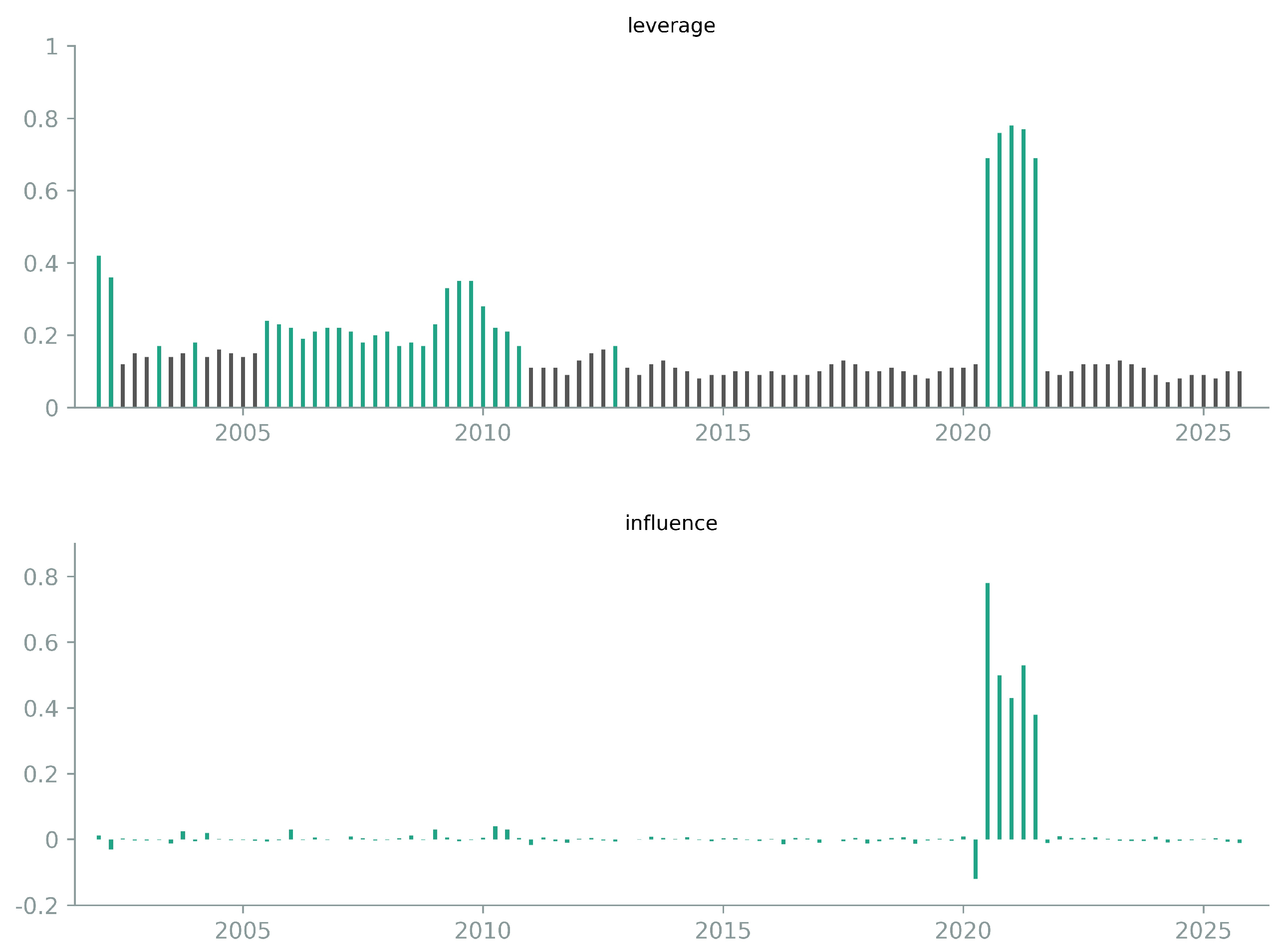
Figure A2.
Residual Plots of the Baseline VECM.
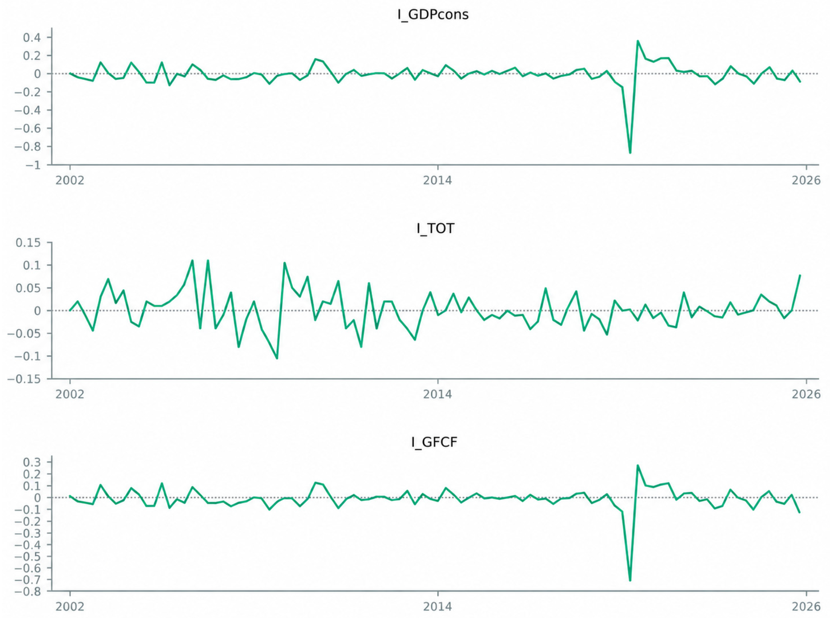
Figure A3.
CUSUM Parameter Stability Test. The green line with circular markers represents the CUSUM statistic, while the two orange lines indicate the upper and lower 95% confidence bounds.
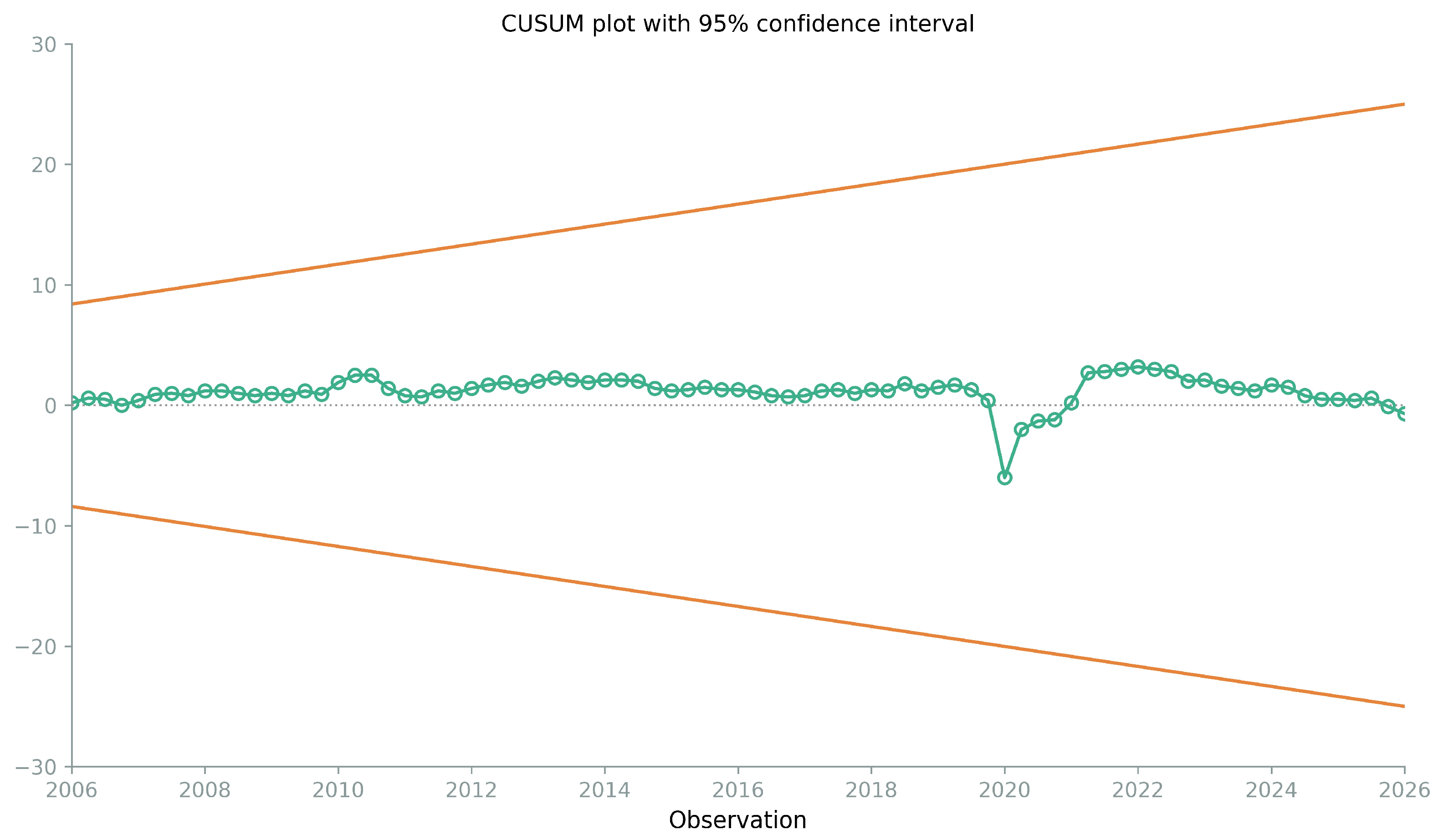
Figure A4.
CUSUMSQ Parameter Stability Test. The green line with circular markers represents the CUSUMSQ statistic, the two solid orange lines indicate the upper and lower 95% confidence bounds, and the dotted orange line represents the reference trajectory.
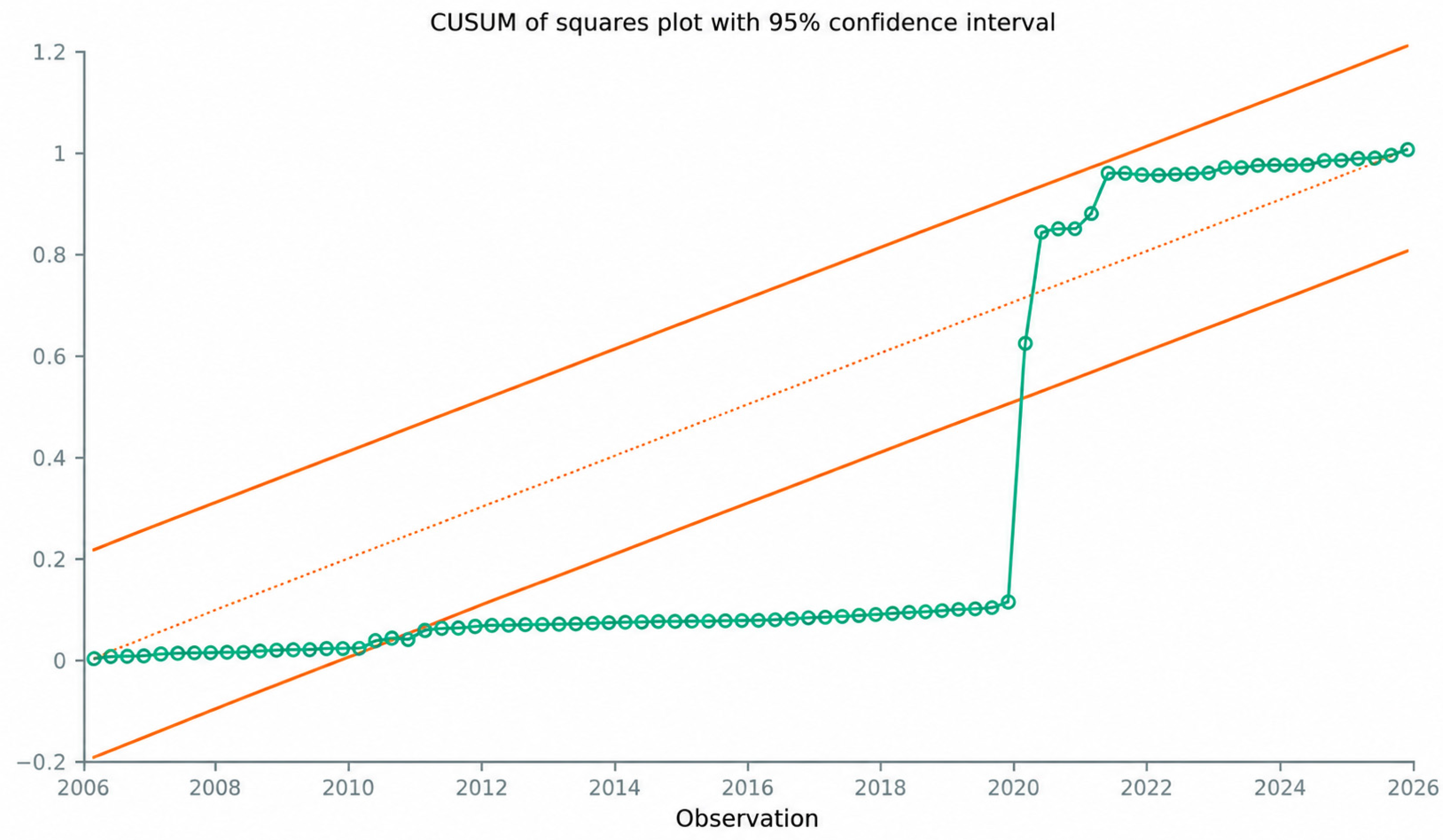
References
- Rolim, L.N.; Lima, G.T.; Baltar, C.T. The impact of international trade shocks on domestic output, income distribution, and inflation in an agent-based model. J. Econ. Interact. Coord. 2025, 20, 843–894. [Google Scholar] [CrossRef] [Scilit]
- Valdes, R. Sub-national economic effects of the resources sector in Chile. J. Appl. Econ. 2021, 24, 141–153. [Google Scholar] [CrossRef] [Scilit]
- Di Pace, F.; Juvenal, L.; Petrella, I. Terms-of-trade shocks are not all alike. Am. Econ. J. Macroecon. 2025, 17, 24–64. [Google Scholar] [CrossRef] [Scilit]
- Sang, J.; Ham, N.-H.; Kim, J.-H.; Kim, J.-J. Impacts of macroeconomic fluctuations on insolvency: Case of Korean construction companies. J. Manag. Eng. 2014, 30, 05014009. [Google Scholar] [CrossRef] [Scilit]
- Banco Central de Reserva del Perú. Producto Bruto Interno por Sectores; Banco Central de Reserva del Perú: Lima, Peru. Available online: https://estadisticas.bcrp.gob.pe/estadisticas/series/anuales/pbi-por-sectores (accessed on 7 July 2026).
- Instituto Nacional de Estadística e Informática. Perú: Comportamiento de los Indicadores del Mercado Laboral a Nivel Nacional; Informe Técnico No. 1; Instituto Nacional de Estadística e Informática (INEI): Lima, Peru, 2025. Available online: https://www.inei.gob.pe/media/MenuRecursivo/boletines/informe-tecnico_empleonacional_1.pdf (accessed on 7 July 2026).
- Al-Tabtabai, H.; Soliman, E. Oil prices drop effect on construction industry in Kuwait. J. Eng. Res. 2022, 10, 1–15. [Google Scholar] [CrossRef] [Scilit]
- Olanipekun, A.O.; Saka, N. Response of the Nigerian construction sector to economic shocks. Constr. Econ. Build. 2019, 19, 160–180. [Google Scholar] [CrossRef] [Scilit]
- Martos, M.; Rodríguez, A. Relationship between Terms of Trade and the GDP of the Mining Sector in Peru, 2000–2023. In LACCEI International Multiconference on Entrepreneurship, Innovation and Regional Development (LEIRD 2025); Virtual Edition, December 1–3; Latin American and Caribbean Consortium of Engineering Institutions (LACCEI): Boca Raton, FL, USA, 2025. [Google Scholar] [CrossRef] [Scilit]
- Rodríguez, A.; Arias, G.; Ocaña, C.; Juárez, H.; García, I. External Terms of Trade and Structural Sustainability in Services Sector: Evidence from Peru. Sustainability 2026, 18, 3134. [Google Scholar] [CrossRef] [Scilit]
- Oviedo, A.; Sierra, L. Importancia de los términos de intercambio en la economía colombiana. Rev. CEPAL 2019, 128, 125–154. [Google Scholar] [CrossRef] [Scilit]
- Škare, M.; Šimurina, J.; Tomić, D. Income terms of trade trend and volatility in Croatia: A growth perspective. Econ. Res.-Ekon. Istraž. 2012, 25, 905–924. [Google Scholar] [CrossRef] [Scilit]
- Schuldt, J. La Enfermedad Holandesa y Otros Virus de la Economía Peruana; Working Paper; Research Center, Universidad del Pacífico: Lima, Peru, 1994; Available online: http://hdl.handle.net/11354/1179 (accessed on 7 July 2026).
- Krugman, P.; Obstfeld, M.; Melitz, M. International Economics: Theory and Policy; Pearson Global Editions: London, UK, 2018. [Google Scholar]
- World Bank. Global Economic Prospects, June 2026; World Bank: Washington, DC, USA, 2026; ISBN 978-1-4648-2315-2. [Google Scholar] [CrossRef] [Scilit]
- Adarov, A.; Kose, A.M.; Vorisek, D. Investment in Emerging and Developing Economies; MPRA Paper No. 127367; Munich Personal RePEc Archive (MPRA), University Library of Munich: Munich, Germany, 2025; Available online: https://mpra.ub.uni-muenchen.de/127367/ (accessed on 7 July 2026).
- Castelblanco, G.; Fenoaltea, E.M.; De Marco, A.; Chiaia, B. Influence of macroeconomic factors on construction costs: An analysis of project cases. Constr. Manag. Econ. 2025, 43, 196–212. [Google Scholar] [CrossRef] [Scilit]
- Chia, F.C.; Skitmore, M.; Runeson, G.; Bridge, A. Economic development and construction productivity in Malaysia. Constr. Manag. Econ. 2014, 32, 874–887. [Google Scholar] [CrossRef] [Scilit]
- Zheng, S.; Liu, H. Interaction among construction investment, other investment and GDP in China. Tsinghua Sci. Technol. 2004, 9, 160–167. [Google Scholar]
- Jiménez-Rodríguez, R.; Morales-Zumaquero, A. Impact of commodity terms-of-trade shocks at disaggregate level. PLoS ONE 2026, 21, e0341374. [Google Scholar] [CrossRef] [Scilit] [PubMed]
- Monterroso, O.; Vilán, D. Commodity terms of trade uncertainty and economic activity in emerging economies. In FEDS Notes; Board of Governors of the Federal Reserve System: Washington, DC, USA, 2025. [Google Scholar] [CrossRef] [Scilit]
- Gazzani, A.; Herrera, V.; Vicondoa, A. The asymmetric effects of commodity price shocks in emerging economies. Eur. Econ. Rev. 2026, 183, 105219. [Google Scholar] [CrossRef] [Scilit]
- Velasquez, C. Terms of Trade and Small Open Economies Business Cycles: The Role of Global Shocks; Working Paper No. 2024-024; Banco Central de Reserva del Perú: Lima, Peru, 2024. Available online: https://www.bcrp.gob.pe/docs/Publicaciones/Documentos-de-Trabajo/2024/documento-de-trabajo-024-2024.pdf (accessed on 21 April 2026).
- Rodríguez, G.; Castillo, P.; Guevara Ruiz, B.; Yamuca Salvatierra, L. Time-varying transmission of external shocks in Peru: Reassessing the role of monetary policy. Econ. Model. 2025, 152, 107241. [Google Scholar] [CrossRef] [Scilit]
- Aguirre López, H.; Carmen Choquehuanca, E.; López León, C.; Padilla Vento, P.; Trujillo Gabriel, C. Shock de los términos de intercambio en la economía peruana, periodo 1994–2021. Rev. Junta 2023, 6, 53–81. [Google Scholar] [CrossRef] [Scilit]
- Khan, M.; Pradhan, M. How do the terms of trade influence economic growth? Evidence from Bangladesh. Int. J. Sustain. Econ. 2022, 14, 250–268. [Google Scholar] [CrossRef] [Scilit]
- Shahzad, U.; He, X.; Muhammad, S. How terms of trade impact economic growth: The case of the United States. SAGE Open 2023, 13, 21582440231176452. [Google Scholar] [CrossRef] [Scilit]
- Dabús, C.; Delbianco, F. Exports, terms of trade and economic growth: Evidence from countries with different level of openness. J. Rev. Glob. Econ. 2019, 8, 327–336. [Google Scholar] [CrossRef] [Scilit]
- Shahzad, U.; Miao, C. Growth in motion: The effects of terms of trade components, labor, capital, and investment on U.S. economic performance. Discov. Sustain. 2025, 6, 381. [Google Scholar] [CrossRef] [Scilit]
- Shahzad, U.; Miao, C. Analysis of Chinese economic growth under technology and consumer components of terms of trade: A time series study (1980–2021). Discov. Sustain. 2025, 6, 1294. [Google Scholar] [CrossRef] [Scilit]
- Makhlouf, Y.; Kellard, N.; Vinogradov, D. What moves commodity terms-of-trade? Evidence from 178 countries. J. Commod. Mark. 2023, 32, 100359. [Google Scholar] [CrossRef] [Scilit]
- Boubakri, S. The asymmetric effect of commodity price returns on economic growth: Evidence from net-commodity-exporting countries during inflationary times. J. Econ. Stud. 2025, 1–15. [Google Scholar] [CrossRef] [Scilit]
- Ben Tahar, M.; Ben Slimane, S.; Houfi, M.A. Commodity prices and economic growth in commodity-dependent countries: New evidence from nonlinear and asymmetric analysis. Resour. Policy 2021, 72, 102043. [Google Scholar] [CrossRef] [Scilit]
- Cavalcanti, T.; Mohaddes, K.; Raissi, M. Commodity price volatility and the sources of growth. J. Appl. Econom. 2015, 30, 857–873. [Google Scholar] [CrossRef] [Scilit]
- Schätz, A. Macroeconomic effects on emerging market sector indices. J. Emerg. Mark. Financ. 2010, 9, 131–169. [Google Scholar] [CrossRef] [Scilit]
- Romero-Ávila, D. Multiple breaks, terms of trade shocks and the unit-root hypothesis for African per capita real GDP. World Dev. 2009, 37, 1051–1068. [Google Scholar] [CrossRef] [Scilit]
- Deb, S. Terms of trade and investment behaviour in Indian agriculture: A cointegration analysis. Indian J. Agric. Econ. 2004, 59, 222–243. [Google Scholar] [CrossRef]
- Ruddock, L.; Lopes, J. The construction sector and economic development: The “Bon curve”. Constr. Manag. Econ. 2006, 24, 717–723. [Google Scholar] [CrossRef] [Scilit]
- Crosthwaite, D. The global construction market: A cross-sectional analysis. Constr. Manag. Econ. 2000, 18, 619–627. [Google Scholar] [CrossRef] [Scilit]
- Lopes, J.; Nunes, A.; Balsa, C. The long-run relationship between the construction sector and the national economy in Cape Verde. Int. J. Strateg. Prop. Manag. 2011, 15, 48–59. [Google Scholar] [CrossRef] [Scilit]
- Nursjanti, F. An analysis of the construction sector and GDP of Indonesia. Int. J. Innov. Creat. Change 2019, 6, 307–316. [Google Scholar]
- Yagual, A.M.; Lopez, M.L.; Sánchez, L.; Narváez, J.G. La contribución del sector de la construcción sobre el producto interno bruto PIB en Ecuador. Rev. Lasallista Investig. 2018, 15, 286–299. [Google Scholar] [CrossRef] [Scilit]
- Sobieraj, J.; Metelski, D. Unveiling economic synchrony: Analyzing lag dynamics between GDP growth and construction activity in Poland and other EU countries. Buildings 2024, 14, 310. [Google Scholar] [CrossRef] [Scilit]
- Qabaja, M.; Tenekeci, G. Nexus between construction sector and economic indicators for Turkey and European Union evidenced by panel data analysis. Eng. Constr. Archit. Manag. 2023, 30, 1978–2007. [Google Scholar] [CrossRef] [Scilit]
- Chiang, Y.H.; Tao, L.; Wong, F.K.W. Causal relationship between construction activities, employment and GDP: The case of Hong Kong. Habitat Int. 2015, 46, 1–12. [Google Scholar] [CrossRef] [Scilit]
- Arora, R.; Kaur, B. Construction activity and economic growth: What follows what? Evidence from India. Int. J. Econ. Policy Emerg. Econ. 2022, 15, 175–196. [Google Scholar] [CrossRef] [Scilit]
- Goh, B.H. Modeling sectoral construction demand and its relationship with economic indicators. Int. J. Constr. Educ. Res. 2012, 8, 223–240. [Google Scholar] [CrossRef] [Scilit]
- Buyukyoran, F.; Yaman, H. Construction sector dynamics in Turkey: Economic advancements and vulnerabilities. J. Constr. Dev. Ctries. 2024, 29, 267–291. [Google Scholar] [CrossRef] [Scilit]
- Ahmad, M.; Jabeen, G.; Hayat, M.K.; Khan, R.E.A.; Qamar, S. Revealing heterogeneous causal links among financial development, construction industry, energy use, and environmental quality across development levels. Environ. Sci. Pollut. Res. 2020, 27, 4976–4996. [Google Scholar] [CrossRef] [Scilit] [PubMed]
- Mallick, H.; Mahalik, M.K. Constructing the economy: The role of construction sector in India’s growth. J. Real Estate Finance Econ. 2010, 40, 368–384. [Google Scholar] [CrossRef] [Scilit]
- Alaloul, W.S.; Musarat, M.A.; Rabbani, M.B.A.; Iqbal, Q.; Maqsoom, A.; Farooq, W. Construction Sector Contribution to Economic Stability: Malaysian GDP Distribution. Sustainability 2021, 13, 5012. [Google Scholar] [CrossRef] [Scilit]
- Abubakar, M.; Abdullahi, M.; Bala, K. Analysis of the causality links between the growth of the construction industry and the growth of the Nigerian economy. J. Constr. Dev. Ctries. 2018, 23, 103–113. [Google Scholar] [CrossRef] [Scilit]
- Saka, N.; Olanipekun, A.O. Impact of the banking sector reform in the construction sector. J. Financ. Manag. Prop. Constr. 2021, 26, 93–112. [Google Scholar] [CrossRef] [Scilit]
- Yorucu, V. Construction in an open economy: Autoregressive distributed lag modeling approach and causality analysis—Case of North Cyprus. J. Constr. Eng. Manag. 2013, 139, 1199–1210. [Google Scholar] [CrossRef] [Scilit]
- Hosein, R.; Lewis, T.M. Quantifying the relationship between aggregate GDP and construction value added in a small petroleum-rich economy: A case study of Trinidad and Tobago. Constr. Manag. Econ. 2005, 23, 185–197. [Google Scholar] [CrossRef] [Scilit]
- Ramsaran, R.; Hosein, R. Growth, employment and the construction industry in Trinidad and Tobago. Constr. Manag. Econ. 2006, 24, 465–474. [Google Scholar] [CrossRef] [Scilit]
- Shiha, A.; El-adaway, I.H. From Ports to Projects: Estimating the Impact of Supply Chain Volatility and Trade Policy Changes on Construction Material Prices. J. Constr. Eng. Manag. 2026, 152, 04026064. [Google Scholar] [CrossRef] [Scilit]
- Lean, C.S. Empirical tests to discern linkages between construction and other economic sectors in Singapore. Constr. Manag. Econ. 2001, 19, 355–363. [Google Scholar] [CrossRef] [Scilit]
- El-adaway, I.H.; Ali, G.G.; Abotaleb, I.S.; Barber, H.M. Studying the relationship between stock prices of publicly traded U.S. construction companies and gross domestic product: Preliminary step toward construction–economy nexus. J. Constr. Eng. Manag. 2020, 146, 04019087. [Google Scholar] [CrossRef] [Scilit]
- Rengifo Calvanapón, G.A.; Sánchez Vallejo, D.A.; Wong Aitken, H.G.; Llaque Fernández, G.I. Cointegración de exportación y crecimiento económico del Perú, periodo 2011–2020. In Proceedings of the 2nd LACCEI International Multiconference on Entrepreneurship, Innovation and Regional Developmen, Virtual, 5–7 December 2022. [Google Scholar] [CrossRef] [Scilit]
- Rodríguez, G.; Villanueva Vega, P.; Castillo Bardalez, P. Driving economic fluctuations in Peru: The role of the terms of trade. Empir. Econ. 2018, 55, 1089–1119. [Google Scholar] [CrossRef] [Scilit]
- Rodríguez, A.; García, H.; Sánchez, I.; Mendoza, C.; Arias, G. Terms of Trade and the Structural Sustainability of the Mining Sector in a Resource-Dependent Economy. Sci 2026, 8, 64. [Google Scholar] [CrossRef] [Scilit]
- Rodríguez, A. Terms of Trade and Structural Sustainability of the Agricultural Sector in Peru: A Cointegration Approach. Agriculture 2026, 16, 6. [Google Scholar] [CrossRef] [Scilit]
- Grytten, O.H. Changes in commodity prices as the factor triggering financial crises. In Elgar Encyclopedia of Financial Crises; Hsu, S., Ed.; Edward Elgar Publishing: Cheltenham, UK, 2023; pp. 70–75. [Google Scholar] [CrossRef] [Scilit]
- Singh, T. Do Terms of Trade Affect Economic Growth? Robust Evidence from India. Econ. Transit. Inst. Change 2023, 31, 491–521. [Google Scholar] [CrossRef] [Scilit]
- Lee, D. Commodity terms of trade volatility and industry growth. Eur. Econ. Rev. 2023, 156, 104479. [Google Scholar] [CrossRef] [Scilit]
- Avom, D.; Kamguia, B.; Ngameni, J.P.; Njangang, H. How does terms of trade volatility affect macroeconomic volatility? The roles of financial development and institutions. Int. Econ. 2021, 168, 98–114. [Google Scholar] [CrossRef] [Scilit]
- Arroyo Marioli, F.; Gootjes, B.; Vasishtha, G. Navigating Volatility: Fiscal Policy and Commodity Price Swings. In Global Economic Prospects, June 2026; World Bank: Washington, DC, USA, 2026; Chapter 4; pp. 121–161. Available online: https://openknowledge.worldbank.org/server/api/core/bitstreams/04c0d880-9100-4e71-8aeb-e65a50725e4c/content (accessed on 11 August 2026).
- Loayza, N.V.; Galego Mendes, A.; Mendez Ramos, F.; Pennings, S.M. Assessing the Effects of Natural Resources on Long-Term Growth: An Extension of the World Bank Long Term Growth Model; Policy Research Working Paper No. 9965; World Bank: Washington, DC, USA, 2022; Available online: http://documents.worldbank.org/curated/en/584811647268984881 (accessed on 14 August 2026).
- Liu, J.; Baek, I.; Noh, S. Commodity terms of trade news and country spreads in emerging economies. Econ. Lett. 2025, 256, 112604. [Google Scholar] [CrossRef] [Scilit]
- Burstein, A.; Neves, J.C.; Rebelo, S. Investment Prices and Exchange Rates: Some Basic Facts; NBER Working Paper No. 10238; National Bureau of Economic Research: Cambridge, MA, USA, 2004. [Google Scholar] [CrossRef] [Scilit]
- Miranda-Pinto, J.; Pescatori, A.; Stuermer, M.; Wang, X. Beyond Energy: Inflationary Effects of Metals Price Shocks in Production Networks; IMF Working Paper No. 24/215; International Monetary Fund: Washington, DC, USA, 2024; Available online: https://www.imf.org/-/media/files/publications/wp/2024/english/wpiea2024215-print-pdf.pdf (accessed on 14 August 2026).
- Gurmu, A. Forecasting building cost index with VECM: Integrating output-based indexes and macroeconomic indicators. J. Eng. Des. Technol. 2026, 24, 1012–1036. [Google Scholar] [CrossRef] [Scilit]
- Engle, R.F.; Granger, C.W.J. Cointegration and Error Correction: Representation, Estimation and Testing. Econometrica 1987, 55, 251–276. [Google Scholar] [CrossRef] [Scilit] [PubMed]
- Said, S.E.; Dickey, D.A. Testing for Unit Roots in Autoregressive-Moving Average Models of Unknown Order. Biometrika 1984, 71, 599–607. [Google Scholar] [CrossRef]
- Kwiatkowski, D.; Phillips, P.C.B.; Schmidt, P.; Shin, Y. Testing the Null Hypothesis of Stationarity against the Alternative of a Unit Root: How Sure Are We That Economic Time Series Have a Unit Root? J. Econom. 1992, 54, 159–178. [Google Scholar] [CrossRef] [Scilit]
- Johansen, S. Statistical Analysis of Cointegration Vectors. J. Econ. Dyn. Control 1988, 12, 231–254. [Google Scholar] [CrossRef] [Scilit]
- Johansen, S. Testing Weak Exogeneity and the Order of Cointegration in UK Money Demand Data. J. Policy Model. 1992, 14, 313–334. [Google Scholar] [CrossRef] [Scilit]
- Zivot, E.; Andrews, D.W.K. Further Evidence on the Great Crash, the Oil-Price Shock, and the Unit-Root Hypothesis. J. Bus. Econ. Stat. 1992, 10, 251–270. [Google Scholar] [CrossRef] [Scilit]
- Glancy, D.; Kurtzman, R.; Loewenstein, L. JUE Insight: Shovel ready projects and commercial construction activity’s long and variable lags. J. Urban Econ. 2026, 151, 103816. [Google Scholar] [CrossRef] [Scilit]
- Fernandes, A.; Rigato, R. K Wasn’t Built in a Day: Investment with Endogenous Time to Build; IMF Working Paper No. 25/78; International Monetary Fund: Washington, DC, USA, 2025; Available online: https://www.imf.org/en/publications/wp/issues/2025/04/11/k-wasnt-built-in-a-day-566136 (accessed on 21 August 2026).
- Caldera Sánchez, A.; Johansson, Å. The Price Responsiveness of Housing Supply in OECD Countries; OECD Economics Department Working Papers No. 837; OECD Publishing: Paris, France, 2011. [Google Scholar] [CrossRef]
- van Wincoop, E. Structural adjustment and the construction sector. Eur. Econ. Rev. 1993, 37, 177–201. [Google Scholar] [CrossRef] [Scilit]
- Rademeyer, M.C.; Minnitt, R.C.A.; Falcon, R.M.S. A characterisation of the mechanisms transforming capital investment into productive capacity in mining projects with long lead-times. Miner. Econ. 2020, 33, 349–357. [Google Scholar] [CrossRef] [Scilit]
- Granger, C.W.J. Some recent development in a concept of causality. J. Econom. 1988, 39, 199–211. [Google Scholar] [CrossRef] [Scilit]
- Masih, R.; Masih, A.M.M. Macroeconomic activity dynamics and Granger causality: New evidence from a small developing economy based on a vector error-correction modelling analysis. Econ. Model. 1996, 13, 407–426. [Google Scholar] [CrossRef] [Scilit]
- Alogoskoufis, G.; Smith, R. On Error Correction Models: Specification, Interpretation, Estimation. J. Econ. Surv. 1991, 5, 97–128. [Google Scholar] [CrossRef] [Scilit]
- Rodríguez, A.; García, H.; Sánchez, I.; Arias, G. Dutch Disease and the Structural Sustainability of the Manufacturing Sector: Empirical Evidence from Peru. Sustainability 2026, 18, 32. [Google Scholar] [CrossRef] [Scilit]
- Karapetyan, N.; Movsisyan, M.; Petrosyan, N.; Mirumyan, A.; Tonoyan, K. Spillovers of construction boom to macroeconomy in a small-open developing economy: The case of Armenia. Proc. Eng. Sci. 2025, 7, 189–198. [Google Scholar] [CrossRef] [Scilit]
- Mendoza, E.G. The terms of trade, the real exchange rate, and economic fluctuations. Int. Econ. Rev. 1995, 36, 101–137. [Google Scholar] [CrossRef] [Scilit]
- Nilavongse, R.; Rubaszek, M.; Staehr, K.; Uddin, G.S. Foreign and domestic uncertainty shocks in four open economies. Open Econ. Rev. 2021, 32, 933–954. [Google Scholar] [CrossRef] [Scilit]
- Petrella, I.; Juvenal, L.; Di Pace, F. Commodity Prices and Fiscal (Pro)Cyclicality; IDB Working Paper No. 1739; Inter-American Development Bank: Washington, DC, USA, 2025. [Google Scholar] [CrossRef] [Scilit]
- Carrière-Swallow, Y.; Magud, N.E. Exchange rate flexibility, the real exchange rate, and adjustment to terms-of-trade shocks. Rev. Int. Econ. 2021, 29, 439–483. [Google Scholar] [CrossRef] [Scilit]
- Vasishtha, G. Fiscal Policy in Commodity Exporters: A Balancing Act; World Bank: Washington, DC, USA, 2026; Available online: https://www.worldbank.org/en/research/publication/fiscal-policy-in-commodity-exporters (accessed on 14 August 2026).
- Kirchberger, M. The Construction Sector in Developing Countries: Some Key Issues. In Mining for Change: Natural Resources and Industry in Africa; Page, J., Tarp, F., Eds.; Oxford University Press: Oxford, UK, 2020; Chapter 3. [Google Scholar] [CrossRef] [Scilit]
- Rodríguez, A.; García, H.; Arias, G.; Sánchez, I. Relación de intercambio y actividad industrial en Perú: Contraste de la enfermedad holandesa. Rev. Cienc. Soc. 2025, 31, 47–66. [Google Scholar] [CrossRef] [Scilit]
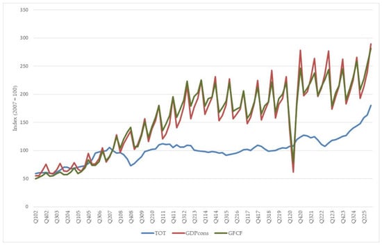
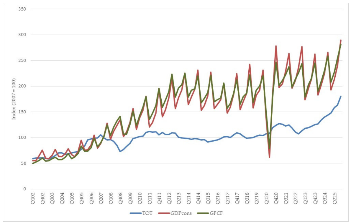

Disclaimer/Publisher’s Note: The statements, opinions and data contained in all publications are solely those of the individual author(s) and contributor(s) and not of MDPI and/or the editor(s). MDPI and/or the editor(s) disclaim responsibility for any injury to people or property resulting from any ideas, methods, instructions or products referred to in the content. |
© 2026 by the authors. Licensee MDPI, Basel, Switzerland. This article is an open access article distributed under the terms and conditions of the Creative Commons Attribution (CC BY) license.