Risk Prioritization of Nearby Infrastructure-Related 311 Requests Around Urban Streetworks Using Public Data: A Weather-Informed Calibrated Random Forest Case Study in New York City

Abstract

Urban streetworks are necessary for infrastructure maintenance and renewal, but they may generate local disruptions that are difficult to observe systematically. This study develops a reproducible public-data-based workflow for prioritizing urban streetwork closure days according to their risk of nearby infrastructure-related 311 service requests (municipal non-emergency reports submitted by residents or other street users). The case study uses New York City data from 2022 to 2024 and integrates recorded street closures, selected 311 complaints, and daily weather variables. A closure day is defined as a recorded street closure active on a single calendar day. The main target identifies whether at least one selected 311 request occurred in the vicinity of an active closure on the same day. The final model is a weather-informed, calibrated Random Forest. The final dataset contained 2,708,620 closure day records. The model achieved an ROC-AUC of 0.6408, a PR-AUC of 0.0799, and a Brier score of 0.0459. Among the top 5% highest-risk closure days, precision reached 11.48%, with a lift of 2.35 over random selection, relative to a 2024 test prevalence of approximately 4.88%. Permutation importance showed that location and calendar features dominated prediction, while continuous weather variables provided a smaller but measurable contribution.

1. Introduction

Urban streetworks cannot be avoided. Cities need them to repair pavements, replace utilities, renew infrastructure, and respond to failures. The problem is that even short works can disturb the everyday use of the street. They may affect various infrastructure users, including drivers, pedestrians, public transport, local businesses, and municipal services.

The scale of this disturbance depends on location and timing. A lane occupation on a quiet local street may have little practical effect. The same occupation near a main junction, bus stop, school, or commercial frontage may quickly become problematic. Traffic intensity, pedestrian activity, land use, season, weekday, weather, etc., can all change the impact of the same type of work. Previous studies on roadworks and work zones have studied their impact on traffic behavior, travel-time reliability, safety, lane-changing, and user discomfort [1,2,3]. In dense urban areas, these effects are harder to separate from background congestion, limited street space, pedestrian flows, utility networks, and differences in how local users report disruptions.

Data on the real effects of streetworks are difficult to collect. The necessary records are usually split between city offices, contractors, utility owners, permit databases, field reports, and traffic management systems. In many cases, project-level data are not public because they contain commercial information, legal constraints, administrative records, or personal data. This is a serious limitation for research on construction and infrastructure management. Many AI (artificial intelligence) studies in the AEC domain are still based on small datasets, single projects, or cases that are difficult to generalize [4,5,6]. With such data, complex models (for example, deep neural networks) may fit the training sample well but fail when tested on new cases [7,8]. For decision support, this is a major problem. A model used in infrastructure planning should not only reproduce past observations. It should remain stable when operating conditions change, and its results should be understandable to planners.

The modeling task becomes harder when the event of interest is rare. In streetwork data, events like reported disruptions, complaints, failures, or safety incidents usually account for only a small share of all observations. In such case, accuracy may give a false impression of model quality. A model can classify most observations correctly, yet still miss the few cases that require action. Research on rare events and imbalanced data shows that target definitions, validation methods, and evaluation metrics must all match the practical use of the model [9,10]. For streetworks, the aim is usually not to predict every disruption perfectly, but to flag a limited number of higher-risk closure days for additional analysis.

Public urban datasets can partly reduce the problem of limited project-level data. Many cities publish open data on permits, street closures, service requests, traffic, weather, and infrastructure assets. These datasets are not perfect, but they are usually much larger and easier to reproduce than internal construction records. Municipal systems, like 311 (a non-emergency telephone number and digital service provided by many local governments in the United States and Canada), could be especially useful. Previous studies have used 311 records to analyze neighborhood conditions, public service demand, and reported local problems [11,12,13]. For this reason, 311 reports can be used as a proxy for visible urban problems (including nuisance and service disruption related to infrastructure works).

However, 311 data need careful interpretation. A 311 request records a reported problem, not every problem experienced by residents, pedestrians, or drivers. Reporting may depend on who notices the issue, who knows how to report it, and who expects the city to respond. Studies on citizen-generated urban data show that unequal reporting can affect data-driven decisions if such reports are treated as neutral evidence [14,15]. For this reason, this study uses selected 311 requests only as a proxy for reported infrastructure-related disruption. They are not treated as a complete or unbiased measure of streetwork impact.

Weather is another factor that matters when analyzing streetwork impacts. Rain, snow, heat, or poor visibility can change traffic conditions, pedestrian comfort, safety, or the way temporary closures are perceived [16,17]. This includes extreme weather, which is studied extensively in research on transport resilience and infrastructure vulnerability [18,19,20]. In the case of streetworks, weather may make a closure or sidewalk occupation more inconvenient than it would be under normal conditions. It may also worsen drainage problems, surface defects, or other local street conditions. For this reason, daily weather variables were included in the model as contextual factors that may help identify higher-risk closure days.

This study focuses on the risk prioritization of urban streetwork impacts using public data. The aim is to identify recorded streetwork days that are more likely to be associated with nearby infrastructure-related 311 service requests. The proposed unit of analysis is the closure day, defined as one recorded street closure active on one calendar day. This unit transforms multiday streetwork records into daily observations. It also makes it possible to combine location, timing, work characteristics, nearby 311 requests, and daily weather conditions in one model.

The case study in this manuscript uses New York City data from 2022 to 2024. It combines three public datasets: recorded street closures, selected infrastructure-related 311 service requests, and daily weather records. The final dataset contains 2,708,620 closure day records. The final model is a calibrated Random Forest with weather variables. It was trained on 2022 data, calibrated on 2023 data, and tested on records from 2024. This time-based split reduces the risk of overly optimistic validation and checks whether the model remains useful in a later operational year. The evaluation covers discrimination, probability calibration, top-risk group precision, recall, lift, feature importance, permutation importance, and sensitivity analysis. The analytical workflow can be reimplemented for other periods or cities with comparable public data, but the fitted model developed in this case study should be interpreted as specific to New York City and requires local validation before transfer.

The research was designed to answer three main research questions:

• Can publicly available urban datasets be integrated into a reproducible closure day framework for estimating the reported impact risk of streetwork activities?
• To what extent do weather variables improve the prediction and prioritization of streetwork-related 311 impact events?
• Which feature groups contribute most to the calibrated risk estimates, and can the final model support the practical prioritization of high-risk streetwork days?

For this purpose, the study introduces closure day as the unit of analysis for studying the reported impacts of urban streetworks. It also proposes a method for building an impact risk target from selected 311 requests located near active street closures. Additionally, the study develops a calibrated Random Forest model with a proper time-aware training, calibration, and testing design. It evaluates the model as a risk prioritization tool and provides an explainable and reproducible case study showing how public urban data can support infrastructure planning under uncertainty.

2. Materials and Methods

2.1. Study Area and Study Period

The case study was conducted for New York City, USA. The city was selected because it has dense urban conditions, frequent street and utility works, a mature 311 service request system, and extensive open data resources. The study period covered three full calendar years, from 1 January 2022 to 31 December 2024. This period was used to construct a time-aware modeling workflow in which 2022 data were used for model training, 2023 data were used for probability calibration, and 2024 data were stored as the final out-of-sample test year.

The use of a full future test year was important for reducing optimistic validation. In operational infrastructure planning, a risk model should be evaluated on data that occur after the model development period, rather than on randomly mixed observations from the same time interval (for example, due to similar weather conditions, holidays, etc.). Therefore, all final model performance measures reported in this study refer to the full 2024 test set (unless stated otherwise).

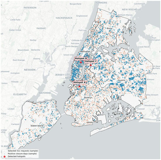
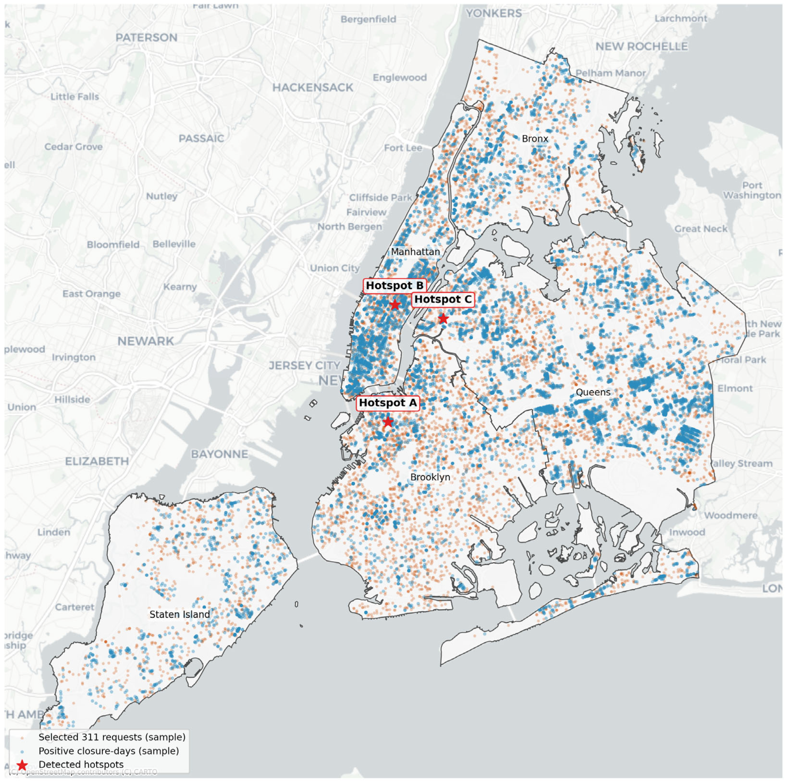
Figure 1 provides a descriptive spatial overview of the analytical target. It shows sampled positive closure days, sampled selected 311 requests, and detected descriptive hotspots. The map was used only for visual interpretation of the spatial structure of the target and was not used as an input to model training, calibration, or testing. Hotspots were identified from local concentrations of positive closure days to illustrate areas with a visibly higher density of nearby reported 311 activity. The hotspots are shown only for visual interpretation and were not used as model inputs.

Figure 1. Spatial distribution of sampled positive closure days, selected 311 requests, and descriptive streetwork-related 311 request hotspots in New York City.

2.2. Data Sources

The model used three public datasets. The first was the New York City street closure dataset, which provided recorded streetwork and street occupation events with start and end dates, borough information, work purpose, street names, and geometries [21]. The second was the New York City 311 Service Requests dataset, from which selected infrastructure-related complaints were extracted [22]. The third was the Open-Meteo Historical Weather API, which provided daily weather variables for the study period [23]. Open-Meteo’s historical API supports the retrieval of historical weather data for specified coordinates and date ranges. It also provides daily variables such as temperature, precipitation, rain, snowfall, wind speed, and wind gusts. Its documentation describes the archive endpoint and the daily weather variables used in this study. The data sources and their roles in the workflow are summarized in Table 1.

Table 1. Data sources and analytical role in the workflow.

Data Source	Provider	Spatial Information	Temporal Information	Main Variables Used	Analytical Role in This Study
Street Closures	NYC Open Data/NYC Department of Transportation	Closure geometry in projected coordinates; street segment location; and borough	Work start and end dates	Closure geometry, borough, work purpose, start date, end date, street names, and closure duration	Construction of the closure day unit of analysis; definition of active streetwork locations and dates
311 Service Requests	NYC Open Data	Request point coordinates; borough; incident address or street name where available	Request creation date and closing date	Complaint type, descriptor, creation date, latitude, longitude, and borough	Construction of the reported impact target by identifying selected infrastructure-related 311 requests near active closures on the same day
Historical Weather Data	Open-Meteo Historical Weather API	Weather query for New York City coordinates	Daily weather records	Maximum, minimum and mean temperature; precipitation; rain; snowfall; maximum wind speed; and wind gusts	Construction of daily weather features and weather stressor indicators for the weather-informed risk model
Derived closure day modeling dataset	Generated in this study	Closure centroid, projected coordinates, borough, and linked spatial context	One record per active closure per calendar day	Closure day ID, closure day, work purpose, duration, calendar variables, weather variables, nearby 311 count, and target variables	Final analytical dataset used for training, calibration, testing, model comparison, and explainability and sensitivity analysis

2.3. Data Preparation and Feature Engineering

Before constructing the modeling dataset, street closure records were cleaned and standardized. Records without valid start or end dates, without usable geometry, or with geometries unsuitable for spatial processing were removed. Records overlapping the study period were retained and clipped to the window from 1 January 2022 to 31 December 2024. Borough names and work purpose categories were standardized to reduce inconsistencies in text fields.

The cleaned closure records were expanded into closure day observations, where each observation represents one recorded street closure active on one calendar day. Calendar variables, including month, weekday, weekend indicator, and season, were derived from the closure day date. Daily weather variables and weather stressor indicators were then joined by calendar date.

Categorical variables were imputed with the most frequent category and one-hot encoded. Numerical variables were imputed with the median and retained in continuous form. Overlapping closure records were not merged into reconstructed physical construction projects; they were treated as administrative closure records from the official dataset. Class imbalance was handled only during model training by retaining all positive training observations and sampling negative observations. Calibration and final testing were performed on the full, unsampled datasets.

2.4. Closure Day Unit of Analysis

The basic unit of analysis was the closure day. A closure day represents one recorded street closure active on one calendar day. So, if a street closure record lasted several days, it generated several closure day observations. This transformation allowed streetwork records with different durations to be represented in a daily based analytical model.

Let $i$ denote a recorded street closure event and let $t$ denote a calendar day. Each closure record has a start date $s_i$, an end date $e_i$, and a geometry $g_i$. The study window is defined as:

$$\mathcal{T}=\{t:t_0\le t\le t_1\}.$$

(1)

In the case study, $t_0$ was 1 January 2022 and $t_1$ was 31 December 2024.

A closure day observation exists for closure $i$ and day $t$ if:

$$t\in [s_i,e_i]\cap \mathcal{T}.$$

(2)

The set of all closure day observations can therefore be written as:

$${\mathcal{D}}_{CD}=\left\{(i,t):t\in [s_i,e_i]\cap \mathcal{T}\right\}.$$

(3)

When applied to the dataset, this operation produced $\mathrm{2,708,620}$ closure day observations from $\mathrm{83,863}$ unique street closure records. Closures that started before 2022 but overlapped the study window were clipped to the study period. Similarly, closures extending beyond 2024 were clipped on 31 December 2024. For each closure day, spatial coordinates, borough, work purpose, raw duration, clipped analysis duration, calendar variables, and later weather variables were retained or constructed.

2.5. Construction of the 311-Based Reported Impact Target

The outcome variable was constructed from selected infrastructure-related 311 service requests. The aim here was not to model all public complaints, but to build a focused proxy for reported streetwork-related or infrastructure-related impact. The selected complaint categories and descriptors included road surface conditions, sidewalk conditions, curb defects, sewer and drainage problems, water-related infrastructure problems, and construction blockage descriptors (Table 2). These categories were selected because they plausibly represent reported local infrastructure-related problems that may be observed near streetwork activity. They do not provide a complete measure of actual streetwork impacts.

Table 2. Selected complaint categories: rationale and interpretation.

311 Request Group	Rationale for Inclusion	Interpretation
Road surface conditions	Potentially visible local street defects or disruption near works	Proxy for reported street surface problems
Sidewalk conditions	Pedestrian space disruption or defects	Proxy for reported pedestrian space problems
Curb defects	Local access/drainage/edge defects	Proxy for reported local street edge problems
Sewer/drainage problems	Possible interaction with excavation, surface water, and weather	Proxy for reported drainage-related problems
Water-related infrastructure problems	Local infrastructure service complaints	Proxy for reported utility-related problems
Construction blockage descriptors	Directly relevant to obstruction or local work inconvenience	Proxy for reported obstruction

Let $r_j$ denote a 311 request, $l_j$ its point location, and ${\tau }_j$ its creation date. Let $d(g_i,l_j)$ denote the spatial distance between closure geometry $g_i$ and request location $l_j$. The main target variable was defined as:

$$y_{i,t}=\left\{\begin{array}{cc}1,& \mathrm{if} \exists r_j \mathrm{such} \mathrm{that} d\left(g_i,l_j\right)\le \rho \mathrm{and} {\tau }_j=t,\\ 0,& \mathrm{otherwise}.\end{array}\right.$$

(4)

where $\rho$ is the spatial matching radius. In the case study, $\rho =150 \mathrm{m}$. Therefore, $y_{i,t}=1$ indicates that at least one selected 311 request occurred within 150 m of an active street closure on the same calendar day.

The count of selected nearby 311 requests was retained:

$$n_{i,t}={\displaystyle \sum _{j=1}^N}\mathbf{1}\left[d\left(g_i,l_j\right)\le \rho \right]\mathbf{1}\left[{\tau }_j=t\right]$$

(5)

where $\mathbf{1}\left[\cdot \right]$ is the indicator function. The target can therefore be extended:

$$y_{i,t}^{\left(q\right)}=\mathbf{1}\left[n_{i,t}\ge q\right],$$

(6)

where $q=1$ for the main target ($y_{i,t}=y_{i,t}^{\left(1\right)}$), and $q=2$ for the sensitivity target ($y_{i,t}^{\left(2\right)}$). This stricter target identifies closure days with at least two selected nearby 311 requests on the same day. It was used only for sensitivity analysis because it is much rarer than the main target.

It is worth noting that 311 requests were treated as a proxy for reported disruption, not as a complete ground-truth measure of actual disruption. This distinction is methodologically important because complaint-based data are affected by reporting behavior, neighborhood context, access to reporting channels, and public awareness [13,14]. The spatial and temporal matching rule used to construct this proxy is described in the following subsection.

2.6. Spatial Processing

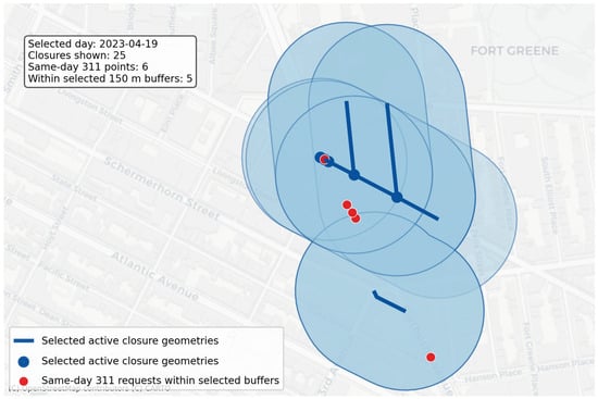
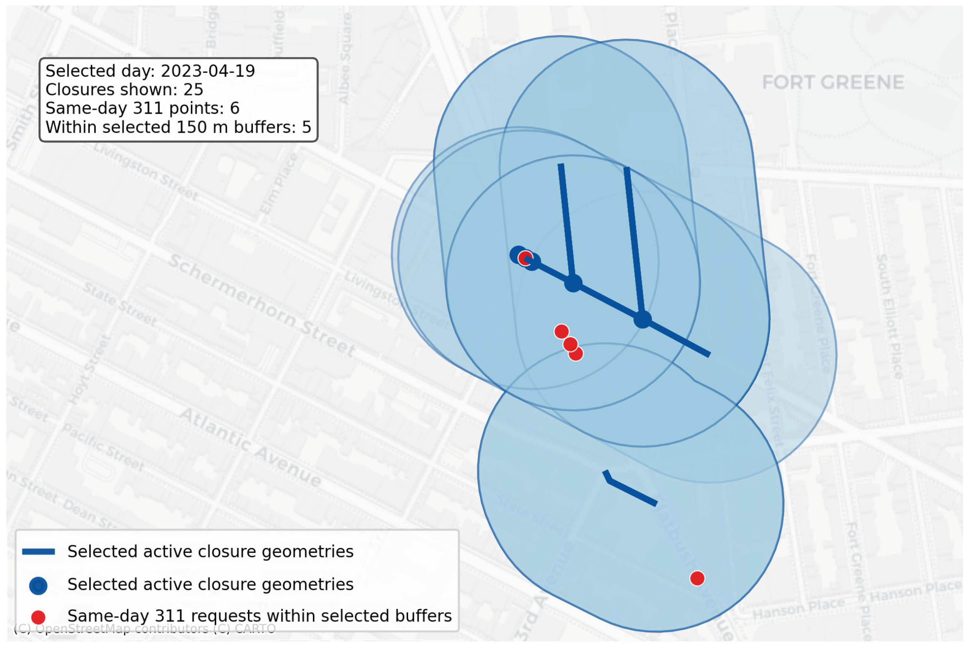
Street closure geometries and 311 request locations were processed in a projected coordinate system suitable for distance calculations in New York City. Closure geometries were used to create 150 m spatial buffers [24,25]. For each calendar day, selected 311 request points were spatially joined to active closure buffers from the same day. The 150 m distance threshold was selected as a strict local impact radius. It captures nearby reported problems while reducing the likelihood that distant 311 requests are attributed to unrelated closures [24,26]. The threshold should be interpreted as an operational modeling assumption rather than a universal physical boundary of streetwork impacts. Figure 2 shows selected active street closure geometries with 150 m buffers. Requests falling within the selected buffers illustrate the spatial–temporal matching rule used to construct the reported impact target.

Figure 2. Illustration of the spatial–temporal target construction logic in a selected hotspot. Active closure geometries were buffered by 150 m, and selected same-day 311 requests falling within the buffers were counted for the corresponding closure day observations.

The matching procedure was designed to construct an operational reported disruption proxy, not to attribute causality. A selected 311 request could be matched to more than one active closure day if the corresponding closure buffers overlapped on the same date. In such cases, the request contributed to the nearby request count of each matching closure day because the modeling unit was the closure day rather than the individual complaint event. This preserves the local exposure structure of the official closure records, but it also means that the target should be interpreted as nearby reported 311 activity, not as a unique causal assignment of a complaint to a specific streetwork activity.

2.7. Weather Variables

Daily weather variables were retrieved for New York City using the Open-Meteo Historical Weather API [23]. The weather data covered the full period from 1 January 2022 to 31 December 2024 and contained no missing daily records in the final weather table. The following daily weather variables were used:

$${\mathbf{w}}_t=\left[T_t^{\mathrm{m}\mathrm{a}\mathrm{x}},T_t^{\mathrm{m}\mathrm{i}\mathrm{n}},T_t^{\mathrm{mean}},P_t,R_t,S_t,V_t^{\mathrm{m}\mathrm{a}\mathrm{x}},G_t^{\mathrm{m}\mathrm{a}\mathrm{x}}\right],$$

(7)

where $T_t^{\mathrm{m}\mathrm{a}\mathrm{x}}$, $T_t^{\mathrm{m}\mathrm{i}\mathrm{n}}$, and $T_t^{\mathrm{mean}}$ denote the maximum, minimum, and mean daily air temperature; $P_t,$ the precipitation sum; $R_t$, the rain sum; $S_t$, the snowfall sum; $V_t^{\mathrm{m}\mathrm{a}\mathrm{x}}$, the maximum wind speed; and $G_t^{\mathrm{m}\mathrm{a}\mathrm{x}}$, the maximum wind gusts.

In addition, binary weather stressor indicators were created:

$${rain}_t=\mathbf{1}[R_t>0],$$

(8)

$${heavyRain}_t=\mathbf{1}[P_t\ge 10],$$

(9)

$${snow}_t=\mathbf{1}[S_t>0],$$

(10)

$${freezing}_t=\mathbf{1}[T_t^{\mathrm{m}\mathrm{i}\mathrm{n}}\le 0],$$

(11)

$${hot}_t=\mathbf{1}[T_t^{\mathrm{m}\mathrm{a}\mathrm{x}}\ge 30],$$

(12)

$${highWind}_t=\mathbf{1}[V_t^{\mathrm{m}\mathrm{a}\mathrm{x}}\ge 10],$$

(13)

All thresholds were used as practical descriptive stressor definitions. They were not intended to represent formal meteorological warning thresholds and can be adjusted for other cases.

2.8. Feature Vector

For each closure day, the model used a feature vector combining spatial, work-related, calendar, and weather variables:

$${\mathbf{x}}_{i,t}=\left[{\mathbf{s}}_i,{\mathbf{u}}_i,{\mathbf{c}}_t,{\mathbf{w}}_t\right],$$

(14)

where ${\mathbf{s}}_i$ represents spatial features, ${\mathbf{u}}_i$ represents work-related features, ${\mathbf{c}}_t$ represents calendar features, and ${\mathbf{w}}_t$ represents daily weather features.

The spatial feature group included borough and projected centroid coordinates. The work-related feature group included closure purpose and duration variables. The calendar group included month, weekday, weekend indicator, and season. The weather group included continuous daily weather variables and binary weather stressor indicators.

Categorical variables were one-hot encoded. Numeric variables were retained in their continuous form. Missing categorical values were imputed with the most frequent category, and missing numerical values were imputed with the median. In the analyzed case, the final weather-informed modeling dataset contained $\mathrm{2,708,620}$ closure day records.

2.9. Time-Aware Modeling Design

The modeling workflow used a time-aware split (training, probability calibration, and final testing):

$${\mathcal{D}}_{train}=\left\{\right(i,t)\in {\mathcal{D}}_{CD}:t\in {\mathcal{T}}_{train}\},$$

(15)

$${\mathcal{D}}_{cal}=\left\{\right(i,t)\in {\mathcal{D}}_{CD}:t\in {\mathcal{T}}_{cal}\},$$

(16)

$${\mathcal{D}}_{test}=\left\{\left(i,t\right)\in {\mathcal{D}}_{CD}:t\in {\mathcal{T}}_{test}\right\}.$$

(17)

In the studied case, ${\mathcal{T}}_{\mathrm{t}\mathrm{r}\mathrm{a}\mathrm{i}\mathrm{n}}$, ${\mathcal{T}}_{\mathrm{c}\mathrm{a}\mathrm{l}}$, and ${\mathcal{T}}_{\mathrm{t}\mathrm{e}\mathrm{s}\mathrm{t}}$ corresponded to 2022, 2023, and 2024, respectively. This design was used to avoid leakage between training, calibration, and testing. It also reflects the intended operational use of the model: learning from past seasons of streetwork and reported impact patterns to prioritize future closure days.

Because the target was rare, controlled negative sampling was used during model training. All positive observations from the training period were retained. A random sample of negative observations was then selected according to a fixed negative-to-positive ratio. The final selected Random Forest used a ratio of 10 negative observations per positive observation during training [27,28]. However, the final evaluation was always conducted on the full, untouched 2024 test set.

Let ${\mathcal{P}}_{train}$ and ${\mathcal{N}}_{train}$ denote the positive and negative observations in the training period. Since $\mid {\mathcal{P}}_{train}\mid \ll \mid {\mathcal{N}}_{train}\mid$, all observations in ${\mathcal{P}}_{train}$ were retained, and a random subset ${\tilde{\mathcal{N}}}_{train}\subset {\mathcal{N}}_{train}$ was sampled for model fitting. This follows the general majority-class under-sampling logic used in imbalanced learning [28]. The sampled training set can be written as:

$${\mathcal{D}}_{fit}={\mathcal{P}}_{train}\cup {\tilde{\mathcal{N}}}_{train}.$$

(18)

where

$$\mid {\tilde{\mathcal{N}}}_{train}\mid =\lambda \mid {\mathcal{P}}_{train}\mid .$$

(19)

As mentioned above, in the final NYC model, $\lambda =10.$ This sampling was used to reduce class imbalance during fitting while preserving an unbiased full-year evaluation on the 2024 data.

2.10. Machine Learning Models

Several models were trained and compared. Logistic regression was used as a simple baseline model. Random Forest models were then used to capture nonlinear effects and interactions among spatial, temporal, work-related, and weather variables. Random Forests are ensemble models that aggregate the predictions of multiple decision trees built with bootstrap sampling and random feature selection [29]. They are commonly used because they can model nonlinear relationships, handle mixed feature types, and provide feature importance measures [29,30].

The Random Forest prediction for a closure day can be represented as the average class probability estimate (raw predicted probability) over $B$ trees:

$${\widehat{\pi }}_{i,t}=f_{RF}({\mathbf{x}}_{i,t})={\displaystyle \frac{1}{B}}{\displaystyle \sum _{b=1}^B}{h}_b({\mathbf{x}}_{i,t}),$$

(20)

where $h_b(\cdot )$ denotes the probability estimate from tree $b$, and $B$ is the number of trees. The final model was a weather-informed Random Forest with the following configuration: $B=400, \max \mathrm{depth}=16, \mathrm{minimum} \mathrm{samples} \mathrm{per} \mathrm{leaf}=50,m_{\mathrm{try}}=\sqrt{d_x},$ where $d_x$ is the number of candidate input features after preprocessing. As mentioned before, the final model used a 10:1 negative-to-positive sampling ratio during training. The implementation used the scikit-learn machine learning library [31].

2.11. Model Selection and Hyperparameter Tuning

Model selection was conducted before the final probability calibration and test set evaluation. The candidate models included a calibrated logistic regression baseline, Random Forest models without weather variables, Random Forest models with weather variables, and sampled Random Forest variants with and without probability calibration. This design allowed comparison between a simple linear baseline, nonlinear tree-based models, and models with or without weather information.

For the Random Forest models, the tuning process considered the number of trees, maximum tree depth, the minimum number of samples per leaf, the feature sampling strategy, and the negative-to-positive sampling ratio used during training. The final selected configuration used 400 trees, a maximum depth of 16, a minimum leaf size of 50, square-root feature sampling, and a 10:1 negative-to-positive sampling ratio.

Model selection was based on the balance between ranking performance and probability reliability. In particular, PR-AUC, top 5% precision, top 5% lift, and the Brier score after calibration were considered. The main selection logic favored models that improved the concentration of positive cases in the highest-risk closure days while maintaining acceptable calibrated probability estimates.

The 2022 data were used for model fitting and candidate model training. The 2023 data were used for probability calibration and for assessing calibrated candidate model behavior during model selection. The 2024 test set was not used for hyperparameter tuning, calibration, or model selection; it was used only once for final evaluation.

2.12. Probability Calibration

Raw classifier scores are not always reliable probability estimates, especially when class imbalance and sampling are involved [32,33]. Probability calibration was therefore applied to transform raw Random Forest probabilities into calibrated risk estimates. Calibration was performed using isotonic regression on the 2023 calibration set. Calibration methods are commonly used to improve the reliability of probabilistic classifiers [32,33].

Let ${\widehat{\pi }}_{i,t}$ denote the raw Random Forest probability. The calibrated predicted probability is:

$${\tilde{\pi }}_{i,t}=c^{\ast }\left({\widehat{\pi }}_{i,t}\right),$$

(21)

where $c^{\ast }(\cdot )$ is a monotonic isotonic calibration function fitted on the calibration set:

$$c^{\ast }=\arg \underset{c\in \mathcal{C}}{\min \sum _{\left(i,t\right)\in {\mathcal{D}}_{cal}}{\left(y_{i,t}-c\left({\widehat{\pi }}_{i,t}\right)\right)}^2},$$

(22)

and $\mathcal{C}$ is the set of non-decreasing calibration functions.

The calibrated probability ${\tilde{\pi }}_{i,t}$ was interpreted as the estimated risk that a given closure day would be associated with at least one selected nearby 311 request on the same day.

2.13. Model Evaluation

Model performance was evaluated on the full 2024 test set. Since the target was rare, evaluation focused on discrimination, calibration, and prioritization rather than on accuracy. The following discrimination metrics were used: $\mathrm{ROC}\text{-}\mathrm{AUC} and \mathrm{PR}\text{-}\mathrm{AUC}.$

ROC-AUC measures the ability of the model to rank positive cases above negative cases across classification thresholds. PR-AUC was chosen as it is especially useful for rare event settings. It focuses on precision and recall for the positive class [34].

Probability calibration was evaluated using the Brier score [35]:

$$\mathrm{Brier}={\displaystyle \frac{1}{\left|{\mathcal{D}}_{test}\right|}}\sum _{\left(i,t\right)\in {\mathcal{D}}_{test}}{\left(y_{i,t}-{\tilde{\pi }}_{i,t}\right)}^2.$$

(23)

Lower Brier scores indicate better calibrated probabilistic predictions [35].

Because the intended use of the model is risk prioritization, top-$k$ metrics were also used. The closure days in the test set were first ranked in descending order of calibrated predicted risk ${\tilde{\pi }}_{i,t}$. Let ${\mathcal{D}}_{\mathrm{t}\mathrm{e}\mathrm{s}\mathrm{t}}$ denote the full test set, and $\alpha \in \left(\mathrm{0,1}\right)$ denote the selected top-risk share (for example $0.01$, $0.05$, or $0.10$), the corresponding number of selected closure days can be defined as:

$$k_{\alpha }=⌈\alpha \left|{\mathcal{D}}_{test}\right|⌉,$$

(24)

Let $K_{\alpha }$ denote the set of the $k_{\alpha }$ closure days with the highest calibrated predicted risk values. Precision at $k_{\alpha }$, recall at $k_{\alpha }$, and lift at $k_{\alpha }$ were defined as follows:

$$Precision@k_{\alpha }={\displaystyle \frac{\sum _{\left(i,t\right)\in K_{\alpha }}{y}_{i,t}}{k_{\alpha }}},$$

(25)

$$Recall@k_{\alpha }={\displaystyle \frac{\sum _{\left(i,t\right)\in K_{\alpha }}{y}_{i,t}}{\sum _{\left(i,t\right)\in {\mathcal{D}}_{test}}{y}_{i,t}}},$$

(26)

$$Lift@k_{\alpha }={\displaystyle \frac{\mathrm{Precision}@k_{\alpha }}{{\bar{y}}_{test}}},$$

(27)

where ${\bar{y}}_{test}$ is the observed positive-class rate in the test set:

$${\bar{y}}_{test}={\displaystyle \frac{1}{\mid {\mathcal{D}}_{test}\mid }}\sum _{(i,t)\in {\mathcal{D}}_{test}}{y}_{i,t}.$$

(28)

Precision measures the fraction of selected high-risk closure days that are true positive cases, and recall measures the fraction of all positive cases in the test set captured within the selected high-risk group [34,36,37,38]. Lift indicates how much more concentrated positive cases are in the selected high-risk group compared with random selection [37,39].

2.14. Explainability Analysis

Two types of feature importance analysis were used. First, impurity-based Random Forest feature importance was extracted from the final model. This measure is useful for initial model inspection but can be biased toward continuous or high-cardinality variables [29,30]. Therefore, permutation importance was also computed on a fixed sample from the 2024 test set. Permutation importance evaluates the change in model performance after randomly permuting a feature or group of features while keeping all other variables unchanged [29,30].

For a feature group $G$, permutation importance was defined as the decrease in PR-AUC after permuting the variables in $G$:

$$I_G=\mathrm{PR}\text{-}\mathrm{AUC}(\mathbf{X},\mathbf{y})-\mathrm{PR}\text{-}\mathrm{AUC}({\mathbf{X}}^{\left[G\right]},\mathbf{y}).$$

(29)

where ${\mathbf{X}}^{\left[G\right]}$ denotes the test feature matrix after randomly permuting the columns belonging to group $G$. The procedure was repeated five times, and the mean decrease in PR-AUC was reported.

The following feature groups were analyzed:

$$\begin{array}{c}{G}_1=\mathrm{location} \mathrm{features};\hfill \\ G_2=\mathrm{calendar} \mathrm{features};\hfill \\ G_3=\mathrm{work} \mathrm{features};\hfill \\ G_5=\mathrm{weather} \mathrm{flag} \mathrm{features};\hfill \\ G_4=\mathrm{weather} \mathrm{numeric} \mathrm{features};\hfill \\ G_6=\mathrm{all} \mathrm{weather} \mathrm{features}.\hfill \end{array}$$

This grouped analysis was used to determine whether weather variables contributed to model performance beyond spatial, calendar, and work-related information.

2.15. Sensitivity Analysis

A sensitivity analysis was performed using a stricter target (previously mentioned in Equation (6)):

$$y_{i,t}^{\left(2\right)}=\mathbf{1}[n_{i,t}\ge 2].$$

(30)

This target identifies closure days with at least two selected nearby 311 requests on the same day. The same final model configuration was used, but the target variable was replaced by $y_{i,t}^{\left(2\right)}$. This test was not intended to replace the main model (because the stricter target is much rarer). It was used to assess whether the workflow could still concentrate higher-impact closure days better than random selection.

3. Results

3.1. Closure Day Dataset and Target Prevalence

The data processing workflow produced a closure day dataset for the full study period. After cleaning, filtering, and clipping street closure records to the study window, the dataset contained 83,863 unique recorded street closures. Expanding these records into daily observations produced 2,708,620 closure day records.

The main target variable identified whether at least one selected infrastructure-related 311 request occurred within the spatial matching radius of an active closure on the same calendar day. In total, 135,831 closure days were positive cases. This corresponds to a target prevalence of 5.0148%. The target was therefore imbalanced. Therefore, the study required imbalance-aware training and evaluation. However, the absolute number of positive observations was large enough to support supervised learning, provided that model performance was assessed with metrics suitable for rare event classification [9,27,38]. Several thresholds were inspected before selecting the target variable (Table 3). Higher thresholds produced substantially lower prevalence. Therefore, thresholds of three or more nearby requests were treated as too sparse for the main model.

Table 3. Target threshold diagnostics for selected 311 requests.

Target Threshold	Target Definition	Positive Closure Days	Share of All Closure Days	Suggested Use
$n_{i,t}\ge 1$	At least one selected 311 request within 150 m on the same day	135,831	5.0148%	Main target
$n_{i,t}\ge 2$	At least two selected 311 requests within 150 m on the same day	19,032	0.7026%	Sensitivity target
$n_{i,t}\ge 3$	At least three selected 311 requests within 150 m on the same day	4964	0.1833%	Too rare for main modeling
$n_{i,t}\ge 4$	At least four selected 311 requests within 150 m on the same day	2093	0.0773%	Descriptive only
$n_{i,t}\ge 5$	At least five selected 311 requests within 150 m on the same day	1002	0.0370%	Descriptive only
$n_{i,t}\ge 10$	At least ten selected 311 requests within 150 m on the same day	212	0.0078%	Extreme cases only

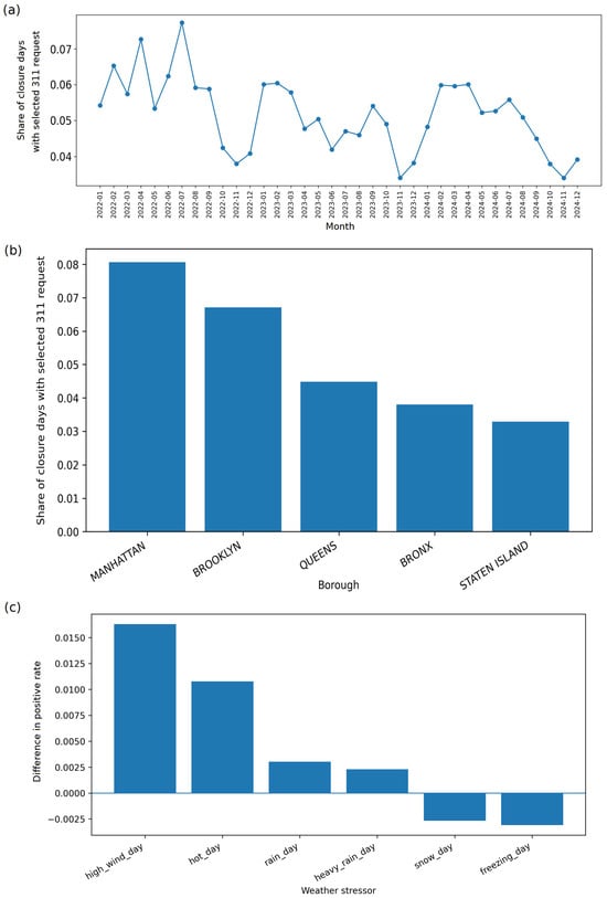
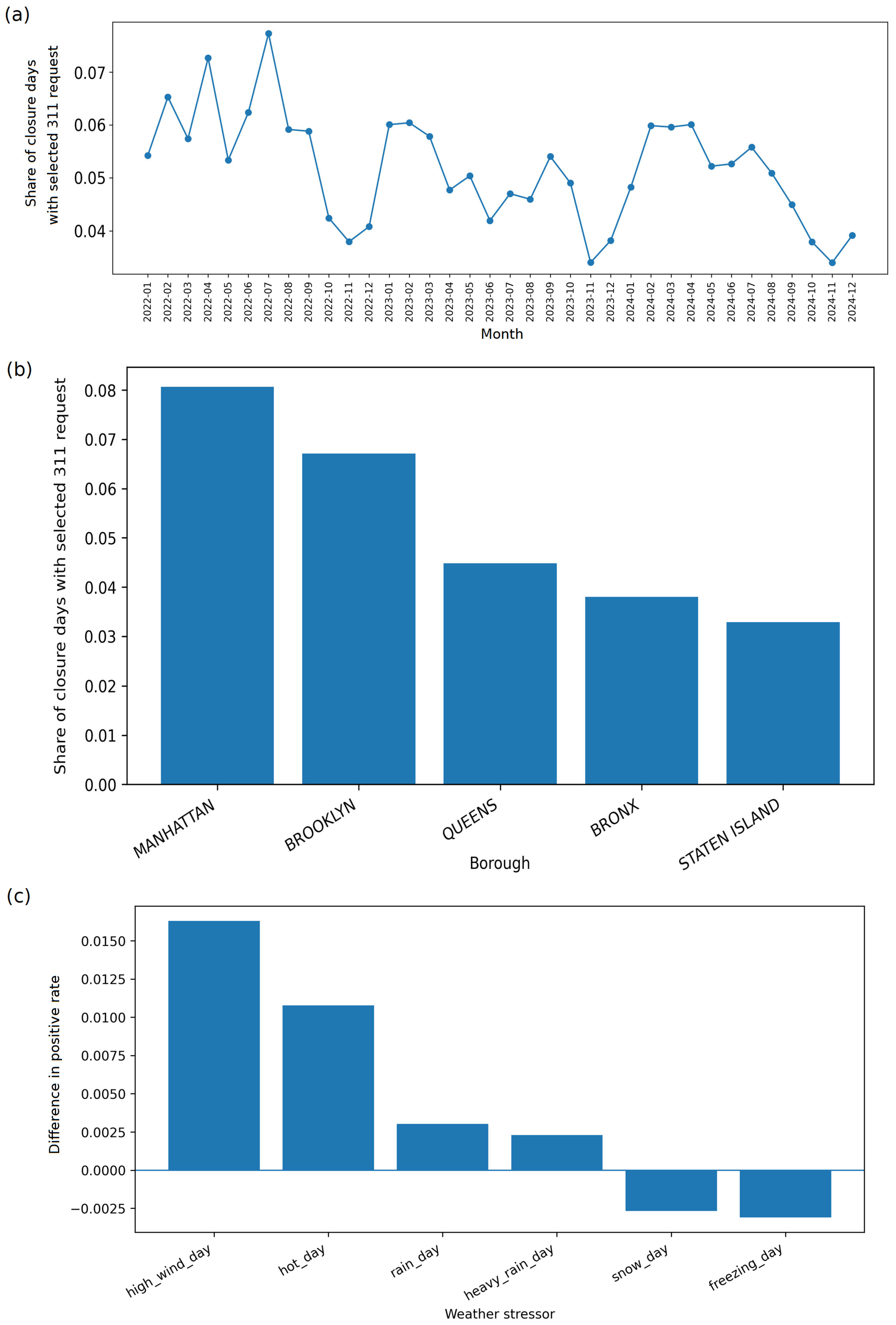
The monthly distribution of the main target showed moderate temporal variability. Monthly positive rates ranged approximately from 3.4% to 7.7%. Higher values were observed in several spring and summer months, while lower values were observed in some of the late autumn and winter months (Figure 3a). This pattern suggests that both seasonal work intensity and public reporting behavior may influence the observed target.

Figure 3. Descriptive variation in the selected nearby 311 request target: (a) monthly target prevalence, (b) target prevalence by borough, and (c) differences in target prevalence on weather stressor days. Values are descriptive associations and should not be interpreted as causal effects.

Borough-level differences were also visible. Manhattan had the highest target prevalence, followed by Brooklyn. Staten Island and the Bronx had lower target prevalence values. These differences indicate that spatial context is an important component of the reported streetwork impact risk. Key borough values are presented in Figure 3b: Manhattan: 8.0658%, Brooklyn: 6.7075%, Queens: 4.4833%, Bronx: 3.8003%, and Staten Island: 3.2875%. According to the study, the dataset shows three important characteristics. First, the closure day framework produced a large analytical panel. Second, the main target was rare enough to require imbalanced learning-aware evaluation, but frequent enough to support model training. Third, the descriptive results already suggest that reported impacts are not randomly distributed. They vary by location and time.

3.2. Weather Conditions and Descriptive Target Differences

Daily weather variables were available for all days in the study period. The weather table contained 1096 daily records and had no missing values (after processing). Weather stressor indicators showed that rain occurred on 530 days, heavy rain on 134 days, snow on 61 days, freezing conditions on 223 days, hot conditions on 115 days, and high-wind conditions on 37 days.

Descriptive comparisons showed that several weather stressors were associated with higher target prevalence. Closure days on rain days had a positive rate of 5.1710%, compared with 4.8687% on non-rain days. Heavy-rain days had a positive rate of 5.2184%, compared with 4.9884% on other days. Hot days had a positive rate of 5.9777%, compared with 4.8991% on non-hot days. High-wind days had the highest descriptive target prevalence, at 6.6064%, compared with 4.9770% on other days. The differences in target prevalence on weather stressor days are presented in Figure 3c.

These results should be interpreted as descriptive associations rather than causal effects. The lower prevalence on snow and freezing days may reflect seasonal differences in streetwork activity, public space use, or reporting behavior. In the author’s opinion, the descriptive weather diagnostics justified the inclusion of weather variables in the predictive workflow.

3.3. Model Comparison

Several models were trained and compared before selecting the final publication-grade model. The comparison included a calibrated logistic baseline, a sampled Random Forest, a calibrated no-weather Random Forest, and a weather-informed calibrated Random Forest.

The calibrated logistic model provided a simple baseline. It achieved an ROC-AUC of 0.6254, a PR-AUC of 0.0718, and a Brier score of 0.0460. Its top 5% precision was 9.27%, corresponding to a lift of 1.90 over random selection.

The sampled Random Forest improved the ranking of high-risk closure days. It achieved a top 5% precision of 11.40% and a lift of 2.34. However, because it was trained on sampled class proportions and not calibrated as the final risk probability model, its Brier score was worse. It was therefore useful as a ranking benchmark but not selected as the main probability model.

The weather- informed calibrated Random Forest improved over the no-weather calibrated Random Forest. The no-weather calibrated Random Forest achieved a top 5% precision of 10.69%, while the weather- informed calibrated Random Forest achieved 11.13%. This indicates that weather variables provided a modest but measurable improvement in prioritizing high-risk closure days. Table 4 reports the comparison of candidate model classes. The final tuned weather-informed calibrated Random Forest is reported separately in Section 3.4 and Table 5.

Table 4. Candidate model comparison before final tuning.

Model	Weather Variables	ROC-AUC	PR- AUC	Brier Score	Top 5% Precision	Top 5% Lift
Calibrated logistic regression	No	0.6254	0.0718	0.0460	9.27%	1.90
Calibrated Random Forest	No	0.6338	0.0779	0.0459	10.69%	2.19
Weather-informed calibrated Random Forest	Yes	0.6394	0.0792	0.0459	11.13%	2.28

Table 5. Final model top-k prioritization performance.

Top-Risk Group	kα: Selected Closure Days	Positive Cases Selected	Precision@kα	Recall@kα	Lift@kα
Top 1%	9358	1300	13.8919%	2.8472%	2.8473
Top 5%	46,792	5371	11.4785%	11.7633%	2.3526
Top 10%	93,583	9884	10.5617%	21.6474%	2.1648

The model comparison shows that the weather-informed calibrated Random Forest offered the strongest balance between ranking performance and probability calibration. In the author’s opinion, this justified its use as the basis for final model tuning.

3.4. Final Weather-Informed Calibrated Random Forest

The final model was selected after controlled tuning of weather-informed Random Forest candidates. The selected model used a negative-to-positive training ratio of 10,400 trees, a maximum tree depth of 16, a minimum leaf size of 50, and square-root feature sampling. The model was trained on the training period, calibrated on the calibration period, and evaluated on the full final test period. The final model achieved an ROC-AUC of 0.640834, a PR-AUC of 0.079906, and a Brier score of 0.045861.

The Brier score indicates that the calibrated probabilities were reliable enough to support risk interpretation at an aggregated level [35,40]. The PR-AUC remained modest in absolute terms, which is expected for a rare event task [34,38]. However, the PR-AUC was higher than the positive-class prevalence in the test set, showing that the model provided useful ranking information [34,41].

Table 5 reports the top-(k) prioritization performance of the final weather-informed calibrated Random Forest.

The top 5% precision of 11.48% should be interpreted in relation to the low base rate of the target. In the 2024 test set, the positive-class prevalence was approximately 4.88%. Therefore, random selection of closure days would be expected to identify positive cases at about this background rate, whereas the model-selected top 5% reached more than twice that concentration. The corresponding lift of 2.35 is a dimensionless enrichment measure relative to random selection. This result does not mean that individual closure days can be predicted with high certainty. Rather, it shows that the model can produce a more informative shortlist of closure days for further review than an unprioritized selection.

3.5. Calibration and Risk Prioritization

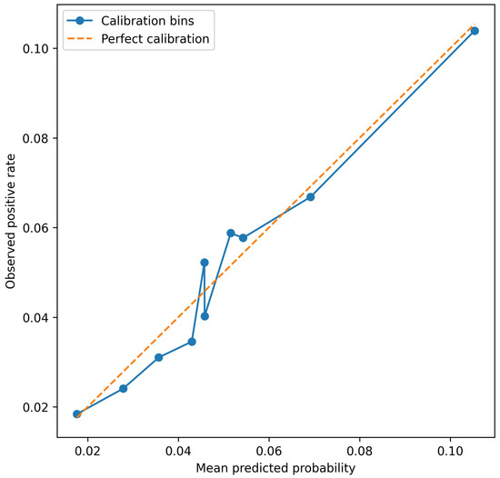
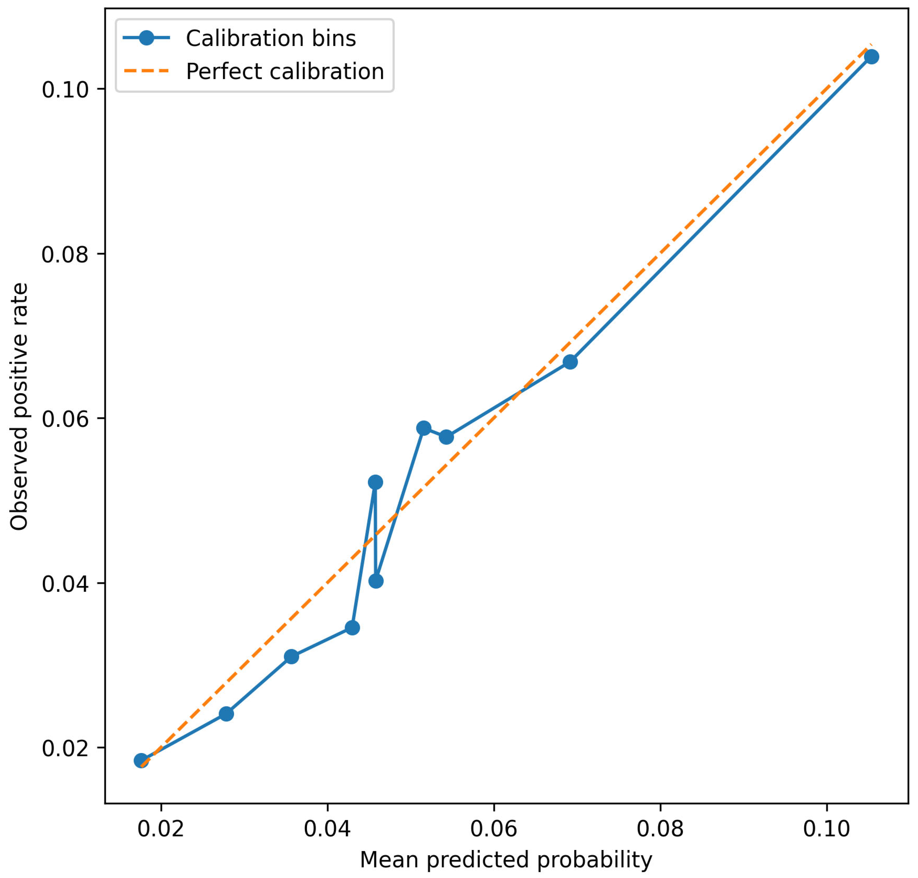
Table 6 and Figure 4 show that predicted probabilities were generally close to observed positive rates across risk bins. This is important because the model is intended to support risk-aware prioritization, not only rank ordering. In the highest-risk decile, the final model produced predicted probabilities that were consistent with the observed rate of positive cases. In the author’s opinion, this clearly supports the claim that the final model should be treated as a calibrated risk model, and not a simple classifier.

Table 6. Calibration table for the final weather-informed calibrated Random Forest.

Risk Decile	Closure Days	Mean Predicted Probability	Observed Positive Rate	Difference	Positive Cases
1	93,584	1.7642%	1.8422%	−0.0780 pp	1724
2	93,583	2.7847%	2.4096%	+0.3751 pp	2255
3	93,583	3.5691%	3.1042%	+0.4649 pp	2905
4	93,584	4.2987%	3.4568%	+0.8419 pp	3235
5	93,583	4.5770%	5.2221%	−0.6451 pp	4887
6	93,583	4.5815%	4.0274%	+0.5541 pp	3769
7	93,584	5.1586%	5.8781%	−0.7195 pp	5501
8	93,583	5.4312%	5.7713%	−0.3402 pp	5401
9	93,583	6.9180%	6.6839%	+0.2341 pp	6255
10	93,584	10.5395%	10.3939%	+0.1456 pp	9727

Figure 4. Calibration plot of the final weather-informed Random Forest.

3.6. Feature Importance and Permutation Importance

The final model was analyzed using both Random Forest feature importance and permutation importance. Impurity-based importance is a standard diagnostic output of Random Forests and provides an initial indication of which predictors contribute to tree splits [29]. However, this measure can be biased toward variables with more potential split points, such as continuous or high-cardinality predictors [42,43]. Therefore, permutation importance was used as the main explainability result. This approach evaluates the decrease in predictive performance after randomly permuting a feature or feature group and is commonly used as a model-agnostic measure of predictive contribution [30,44].

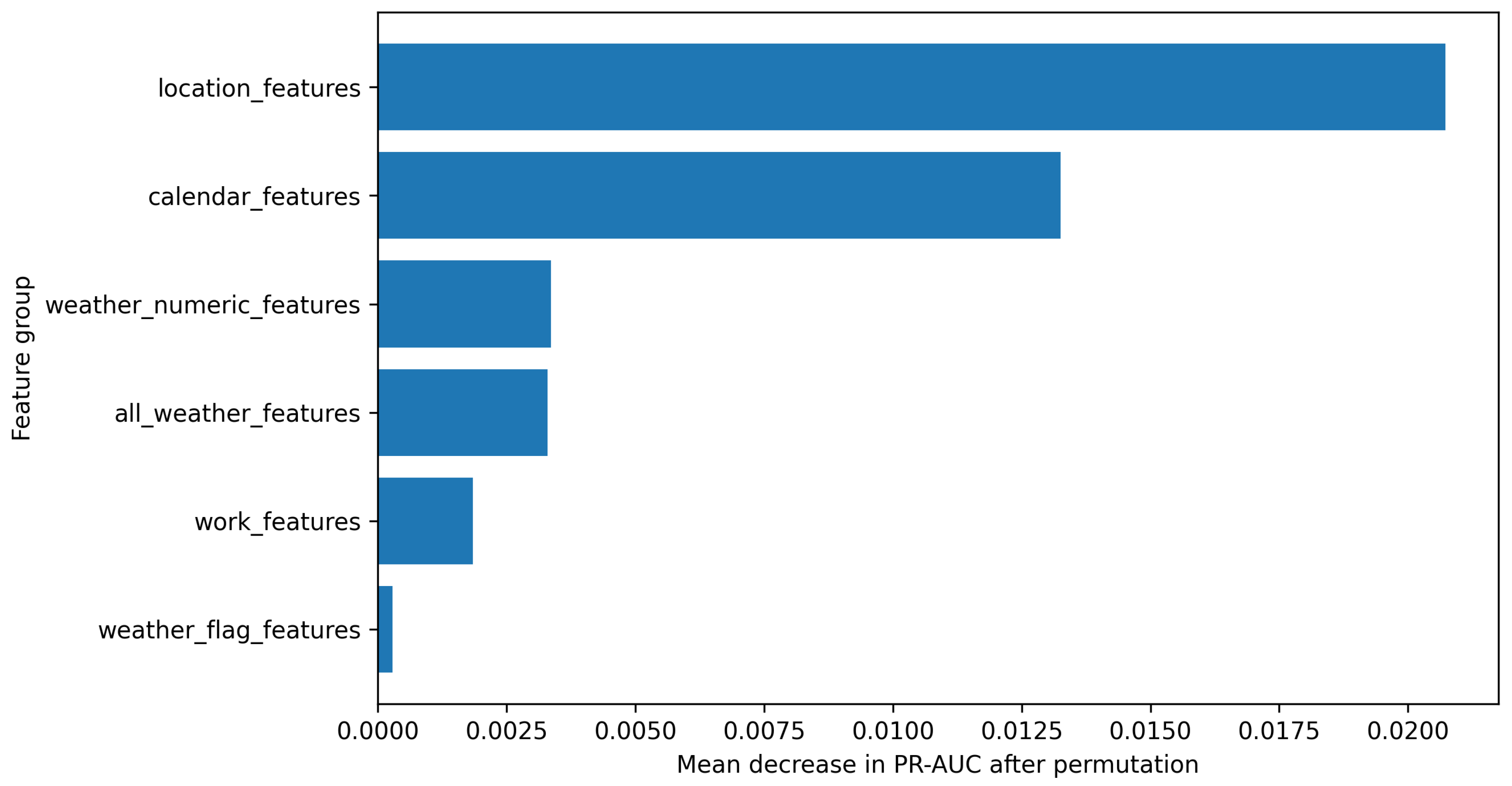
The grouped permutation importance analysis (results presented in Figure 5) showed that location features were the strongest contributor to model performance. Permuting location features reduced PR-AUC by 0.020721 on average. Calendar features were the second-most important group, with a PR-AUC decrease of 0.013258. Weather numeric features were the third-strongest group, with a PR-AUC decrease of 0.003367. Work features had a smaller but positive contribution, with a PR-AUC decrease of 0.001854. Weather flag features had only a weak contribution.

Figure 5. Grouped permutation importance of the final weather-informed calibrated Random Forest, measured as the mean decrease in PR-AUC after permuting each feature group.

The individual permutation importance results confirmed the grouped pattern (Table A1 in Appendix A). The strongest predictors were projected spatial coordinates, weekend indicator, borough, weekday, month, temperature variables, duration variables, and work purpose. These results indicate that the model mainly learned spatial and temporal patterns in nearby reported 311 activities, while weather and work-related features added smaller contextual information. The importance values should be interpreted as predictive contributions to the model, not as causal effects of the corresponding variables.

3.7. Sensitivity Analysis for a Stricter Target

A sensitivity analysis was performed using the stricter target $y_{i,t}^{\left(2\right)}$, which identifies closure days with at least two selected nearby 311 requests on the same day (Equation (6)). This target was much rarer than the main target. Its overall prevalence was 0.7026%, with annual values of 0.7734%, 0.6304%, and 0.7213% in the three study years, respectively.

The sensitivity model was evaluated using the same final Random Forest configuration. Because the stricter target was much rarer, absolute precision values were lower. However, lift values were high, showing that the model still concentrated higher-impact cases better than random selection (Table 7).

Table 7. Sensitivity analysis: top-k prioritization performance for the stricter target.

Top-Risk Group	kα: Selected Closure Days	Positive Cases Selected	Precision@kα	Recall@kα	Lift@kα
Top 1%	9358	322	3.4409%	4.7704%	4.7705
Top 5%	46,792	1002	2.1414%	14.8444%	2.9689
Top 10%	93,583	1682	1.7973%	24.9185%	2.4919

The sensitivity analysis supports the robustness of the prioritization concept. Even when the tested target was made substantially stricter and rarer, the model still identified closure days with a higher-than-average concentration of reported impact events. However, calibration for the stricter target was weaker in the highest-risk decile, where the model tended to overpredict the observed rate. That is why the stricter target is best interpreted as a robustness check, not as the main modeling objective [32,45,46].

4. Discussion

4.1. Interpretation of the Main Findings

The results show that public urban data can be used to develop a reproducible streetwork impact risk prioritization workflow. The closure day unit allowed street closures, selected 311 requests, timing, location, work characteristics, and weather to be combined in one dataset. This is useful because many construction and infrastructure management studies still depend on small or project-specific datasets [4,5,6]. Such data can make it difficult to generalize the results and may increase the risk of overfitting (when machine learning models are used).

The presented final weather-informed calibrated Random Forest did not predict disruptions with certainty. This is not expected (or even possible) in a dense urban setting, where reported impacts depend on local infrastructure conditions, user behavior, reporting habits, public awareness, weather, street context, etc. However, the model is useful as a risk-ranking tool. In the 2024 test year, the top 5% highest-risk closure days contained more than 2.35 times as many positive cases as random selection would suggest. Such model could be useful for municipal planning because agencies usually have limited resources for inspection, coordination, communication, and mitigation.

The ROC-AUC and PR-AUC values should be interpreted in relation to the aim of the model. The target was rare, and the model was designed to rank closure days by risk, not to classify every case correctly. In such problems, AUC values may look moderate even when the model is useful for selecting high-risk cases. For this reason, the top-k results are important. They show whether the model can identify the closure days that should receive attention first. This is consistent with studies on rare event and imbalanced data, which emphasize that standard accuracy is often inappropriate when the positive class is rare [9,10].

4.2. Public Data and the 311 Proxy

One of the main contributions of this study is that the workflow uses only public data. The model was built from open street closure records, 311 service requests, and daily weather data. These data are not perfect, but they allow a large and transparent analysis. The final dataset contained more than 2.7 million closure day observations, which made it possible to test the model on subsequent years’ data. Thanks to that, author did not have to rely on random cross-validation. The time-aware split reflects the practical side of applying a model trained on past data to future streetwork conditions.

The use of 311 requests is both a strength and a limitation of this research. These records provide many observations with location and date information about reported urban problems. Previous studies have used them to analyze urban conditions, service demand, neighborhood distress, and reporting patterns [11,12,13]. At the same time, 311 data are not a complete record of all problems. A request shows that someone reported an issue. It does not show every inconvenience experienced by residents or street users. Reporting may depend on local conditions, access to digital tools, trust in the city, and residents’ willingness to complain [14,15]. For this reason, the model should be understood as a model of reported infrastructure-related impact risk. It can identify closure days with a higher probability of nearby 311 activity, but it cannot prove that a closure caused a complaint or detect problems that were not reported. In practice, it should help select cases for review, not make decisions automatically.

4.3. Weather, Spatial Context, and Feature Contributions

The feature importance results show that the model relied primarily on spatial and calendar information. Location features were the strongest group in the grouped permutation analysis, and projected coordinates and borough also appeared among the most important individual predictors. This is plausible because location may capture several factors that are not directly observed in the dataset, including street hierarchy, density, land use, pedestrian and traffic exposure, utility concentration, infrastructure condition, and local reporting behavior.

Calendar variables were the second-strongest feature group. Their contribution may reflect weekday–weekend differences, seasonal construction cycles, mobility routines, public space use, and seasonal reporting patterns. For practical infrastructure management, this means that reported 311 activity around streetworks is not randomly distributed across time. Some periods and days are more likely to generate nearby reports, even when the same type of closure is considered.

Weather variables provided a smaller but measurable contribution. The comparison between models with and without weather variables showed only an incremental improvement, and the permutation results confirmed that weather was less influential than location and calendar features. However, continuous weather variables, especially temperature-related measures, were more informative than simple binary weather stressor flags. This suggests that weather effects may be gradual, nonlinear, and context-dependent rather than fully captured by fixed thresholds such as rain days, hot days, or high-wind days.

The limited contribution of work-related features should also be interpreted cautiously. Work purpose and duration variables did add information, but their importance was lower than that of spatial and calendar variables. This may reflect the coarse administrative nature of public street closure records. Public work purpose categories may not fully describe the actual intensity, site layout, contractor activity, traffic management arrangement, or construction method used on a given closure day.

Overall, the feature importance results should not be interpreted causally. A high-risk location in the model may reflect genuine infrastructure vulnerability, high user exposure, repeated streetwork activity, stronger public awareness, higher reporting propensity, or a combination of these factors. The model therefore provides a prioritization signal for nearby reported 311 activity, not an explanation of the causal mechanism behind each report.

4.4. Practical Implications

The proposed model is most useful as a screening and prioritization layer. It can help infrastructure agencies identify closure days with an elevated probability of nearby infrastructure-related 311 requests and select a smaller group of cases for further review. In practice, such cases could be checked for overlapping works, field inspection needs, temporary signage, pedestrian or traffic management issues, public communication needs, or contractor coordination.

The practical value of the model lies in enrichment rather than deterministic prediction. In the 2024 test set, the top 5% highest-risk closure days had a precision of 11.48%, compared with an overall positive-class prevalence of approximately 4.88%. This means that the model-selected shortlist contained more than twice the concentration of positive cases expected under random selection. For an agency with limited inspection or coordination capacity, such enrichment can be useful because it helps focus attention on a manageable subset of closure days.

At the same time, this level of precision is not sufficient for automatic enforcement, automatic intervention, or the direct attribution of responsibility. The model should not be used to penalize contractors, neighborhoods, or work types without additional evidence. Its role is to support human review by indicating where reported risk conditions are elevated.

The calibrated probabilities also make the output easier to communicate. Closure days may be grouped into low-, moderate-, and high-risk bands for planning purposes, provided that these bands are validated locally. Such risk bands could support municipal dashboards, inspection scheduling, coordination meetings, or targeted public communication. However, the thresholds used for operational action should be selected by the responsible agency according to available resources, acceptable false-positive rates, and local policy priorities.

4.5. Sensitivity Analysis and Robustness

The stricter sensitivity target required at least two nearby selected 311 requests. This reduced the target prevalence to about 0.7%, making the task harder and precision values lower. Nevertheless, the calibrated model still concentrated stricter positive cases in the highest-risk groups. In the 2024 test year, the top 5% highest-risk closure days had almost three times as many stricter positive cases as random selection.

This result supports the robustness of the general workflow. The proposed model can also rank closure days with a higher concentration of nearby reports. However, calibration was weaker for the stricter target in the highest decile, where the model overpredicted the observed rate. For this reason, the stricter target should be treated as a sensitivity check, not as the main model for practical use.

4.6. Limitations and Future Research

Author must acknowledge several limitations of the study. First, selected 311 requests are only a proxy for reported infrastructure-related disruption. They do not include issues like unreported problems, construction costs, traffic delays, business losses, pedestrian inconvenience, and safety outcomes. Moreover, the study does not prove causality. A 311 request near an active closure may be linked to the closure, but it may also result from older infrastructure problems, other nearby works, weather, or local reporting habits. The model estimates association-based risk, not causal impact.

Additionally, the spatial matching in the case study uses a fixed radius. The chosen range is simple and easy to interpret, but real disruption areas may differ depending on aspects like the type of work, pedestrian movement, traffic conditions, and urban form. Weather was represented by city-level daily variables, so local storms, drainage problems, and microclimatic differences may be missed. Street closure records may also contain duplicates, overlapping permits, or several records for the same physical work area. Finally, the distinction between workflow transferability and model transferability is important. The proposed analytical workflow can be adapted to other cities if comparable data are available, including streetwork or closure records, geocoded service requests or complaint data, and local weather observations. However, the fitted model developed in this study is specific to New York City. Other jurisdictions may differ in reporting behavior, streetwork management practices, infrastructure condition, urban density, data quality, complaint categories, and weather patterns. Therefore, any transfer of the approach should involve local target definition, recalibration, and out-of-sample validation before operational use.

Future research should test other spatial definitions, including road network distances and exposure zones based on street hierarchy. Future work should also include spatially blocked validation, for example, by holding out selected boroughs or spatial grid cells, to evaluate whether the workflow can support prediction in areas that were not used during model development. The following model could also include data like traffic speeds, pedestrian counts, transit disruptions, land use, population density, and/or infrastructure asset data. Future studies could also use causal designs, such as matched comparisons or difference-in-differences, to separate the effect of streetworks from normal neighborhood reporting patterns [47,48]. Calibrated risk scores could be added to municipal planning dashboards to support coordination, inspections, scheduling, public communication, or contractor oversight.

5. Conclusions

This study developed and evaluated a reproducible public-data-based workflow for prioritizing urban streetwork closure days according to the risk of nearby infrastructure-related 311 service requests. The case study showed that recorded street closures, selected 311 requests, daily weather variables, and calendar and spatial information can be integrated into a closure day analytical framework. In the New York City case study, this process produced 2,708,620 closure day observations and provided a scalable structure for constructing and testing reported risk proxies around streetwork activities.

The final weather-informed calibrated Random Forest supported risk prioritization rather than deterministic prediction. On the full 2024 test set, the model achieved an ROC-AUC of 0.6408, a PR-AUC of 0.0799, and a Brier score of 0.0459. In the top 5% highest-risk closure days, precision reached 11.48%, recall reached 11.76%, and lift reached 2.35 over random selection. These results indicate that the model can concentrate nearby reported 311 events in a smaller operational shortlist, although it should not be used as an automatic decision-making or causal attribution tool.

The comparison of models with and without weather variables showed that weather information provided a modest but measurable improvement. Weather did not dominate the prediction problem. The explainability analysis showed that location and calendar features were the strongest contributors to model performance, while continuous weather variables added smaller contextual information. This suggests that the risk of nearby reported 311 activity around streetworks is shaped mainly by where and when a closure occurs, with weather acting as an additional contextual factor.

The sensitivity analysis with a stricter target, based on at least two nearby selected 311 requests, confirmed the robustness of the prioritization concept under a rarer target definition. Although absolute precision was lower because the stricter target was much less frequent, the model still achieved substantial lift in the highest-risk groups. This supports the use of the proposed workflow as a screening layer for reported risk prioritization.

The workflow may be adapted to other cities with comparable public data, but the fitted model should be treated as specific to New York City. Any transfer to another jurisdiction should involve local target definition, recalibration, and out-of-sample validation. Overall, the proposed approach provides a transparent and reproducible basis for identifying streetwork closure days that deserve closer operational review.

References

- Edara, P.; Sun, C.; Zhu, Z. Evaluation of variable advisory speed limits in congested work zones. J. Transp. Saf. Secur. 2017, 9, 123–145. [Google Scholar]
- Jamous, W.; Balijepalli, C.; Watling, D. Assessing travel time reliability implications due to roadworks on private vehicles and public transport services in urban road networks. J. Traffic Transp. Eng. 2018, 5, 296–308. [Google Scholar] [CrossRef] [Scilit]
- Meng, Q.; Weng, J. Evaluation of rear-end crash risk at work zone using work zone traffic data. Accid. Anal. Prev. 2011, 43, 1291–1300. [Google Scholar] [CrossRef] [Scilit] [PubMed]
- Abioye, S.O.; Oyedele, L.O.; Akanbi, L.; Ajayi, A.; Delgado, J.M.D.; Bilal, M.; Akinade, O.O.; Ahmed, A. Artificial intelligence in the construction industry: A review of present status, opportunities and future challenges. J. Build. Eng. 2021, 44, 103299. [Google Scholar] [CrossRef] [Scilit]
- Darko, A.; Chan, A.P.C.; Adabre, M.A.; Edwards, D.J.; Hosseini, M.R.; Ameyaw, E.E. Artificial intelligence in the AEC industry: Scientometric analysis and visualization of research activities. Autom. Constr. 2020, 112, 103081. [Google Scholar] [CrossRef] [Scilit]
- Pan, Y.; Zhang, L. Roles of artificial intelligence in construction engineering and management: A critical review and future trends. Autom. Constr. 2021, 122, 103517. [Google Scholar] [CrossRef] [Scilit]
- Goodfellow, I.; Bengio, Y.; Courville, A. Deep Learning; MIT Press: Cambridge, MA, USA, 2016. [Google Scholar]
- Hastie, T.; Tibshirani, R.; Friedman, J. The Elements of Statistical Learning: Data Mining, Inference, and Prediction, 2nd ed.; Springer: New York, NY, USA, 2009. [Google Scholar]
- He, H.; Garcia, E.A. Learning from imbalanced data. IEEE Trans. Knowl. Data Eng. 2009, 21, 1263–1284. [Google Scholar] [CrossRef] [Scilit]
- King, G.; Zeng, L. Logistic regression in rare events data. Political Anal. 2001, 9, 137–163. [Google Scholar] [CrossRef] [Scilit]
- Li, Y.; Hyder, A.; Southerland, L.T.; Hammond, G.; Porr, A.; Miller, H.J. 311 service requests as indicators of neighborhood distress and opioid use disorder. Sci. Rep. 2020, 10, 19579. [Google Scholar] [CrossRef] [Scilit] [PubMed]
- Stowers, G.N.L. Back to basics: City services and 311 service requests. State Local Gov. Rev. 2022, 54, 13–31. [Google Scholar]
- Wang, L.; Qian, C.; Kats, P.; Kontokosta, C.E.; Sobolevsky, S. Structure of 311 service requests as a signature of urban location. PLoS ONE 2017, 12, e0186314. [Google Scholar] [CrossRef] [Scilit] [PubMed]
- Kontokosta, C.E.; Hong, B. Bias in smart city governance: How socio-spatial disparities in 311 complaint behavior impact the fairness of data-driven decisions. Sustain. Cities Soc. 2021, 64, 102503. [Google Scholar] [CrossRef] [Scilit]
- White, A.; Trump, K.-S. The promises and pitfalls of 311 data. Urban Aff. Rev. 2018, 54, 794–823. [Google Scholar]
- Böcker, L.; Dijst, M.; Prillwitz, J. Impact of everyday weather on individual daily travel behaviours in perspective: A literature review. Transp. Rev. 2013, 33, 71–91. [Google Scholar] [CrossRef] [Scilit]
- Koetse, M.J.; Rietveld, P. The impact of climate change and weather on transport: An overview of empirical findings. Transp. Res. Part D Transp. Environ. 2009, 14, 205–221. [Google Scholar] [CrossRef] [Scilit]
- Ji, T.; Zhu, Y.; Xu, J.; Wang, Y. The impact of climate change on urban transportation resilience to compound extreme events. Sustainability 2022, 14, 3880. [Google Scholar] [CrossRef] [Scilit]
- Markolf, S.A.; Hoehne, C.; Fraser, A.; Chester, M.V.; Underwood, B.S. Transportation resilience to climate change and extreme weather events: Beyond risk and robustness. Transp. Policy 2019, 74, 174–186. [Google Scholar] [CrossRef] [Scilit]
- Pregnolato, M.; Ford, A.; Robson, C.; Glenis, V.; Barr, S.; Dawson, R. Assessing urban strategies for reducing the impacts of extreme weather on infrastructure networks. R. Soc. Open Sci. 2016, 3, 160023. [Google Scholar] [CrossRef] [Scilit] [PubMed]
- NYC Open Data. Street Closures; New York City Open Data: New York, NY, USA, 2026. Available online: https://data.cityofnewyork.us/Transportation/Street-Closures-due-to-Construction-Activities-by-/i6b5-j7bu/about_data/ (accessed on 4 May 2026).
- NYC Open Data. 311 Service Requests from 2020 to Present; New York City Open Data: New York, NY, USA, 2026. Available online: https://data.cityofnewyork.us/Social-Services/311-Service-Requests-from-2020-to-Present/erm2-nwe9/about_data/ (accessed on 4 May 2026).
- Open-Meteo. Historical Weather API Documentation. Open-Meteo. Available online: https://open-meteo.com/ (accessed on 4 May 2026).
- EPSG Geodetic Parameter Dataset. NAD83/New York Long Island (ftUS), EPSG:2263. Available online: https://epsg.io/2263 (accessed on 4 May 2026).
- GeoPandas Developers. Projections—GeoPandas Documentation. Available online: https://geopandas.org/en/stable/docs/user_guide/projections.html (accessed on 4 May 2026).
- Tobler, W.R. A computer movie simulating urban growth in the Detroit region. Econ. Geogr. 1970, 46, 234–240. [Google Scholar] [CrossRef] [Scilit]
- Buda, M.; Maki, A.; Mazurowski, M.A. A systematic study of the class imbalance problem in convolutional neural networks. Neural Netw. 2018, 106, 249–259. [Google Scholar] [CrossRef] [Scilit] [PubMed]
- Lemaître, G.; Nogueira, F.; Aridas, C.K. Imbalanced-learn: A Python Toolbox to Tackle the Curse of Imbalanced Datasets in Machine Learning. J. Mach. Learn. Res. 2017, 18, 1–5. [Google Scholar]
- Breiman, L. Random forests. Mach. Learn. 2001, 45, 5–32. [Google Scholar] [CrossRef] [Scilit]
- Fisher, A.; Rudin, C.; Dominici, F. All models are wrong, but many are useful: Learning a variable’s importance by studying an entire class of prediction models simultaneously. J. Mach. Learn. Res. 2019, 20, 1–81. [Google Scholar]
- Pedregosa, F.; Varoquaux, G.; Gramfort, A.; Michel, V.; Thirion, B.; Grisel, O.; Blondel, M.; Prettenhofer, P.; Weiss, R.; Dubourg, V.; et al. Scikit-learn: Machine learning in Python. J. Mach. Learn. Res. 2011, 12, 2825–2830. [Google Scholar]
- Niculescu-Mizil, A.; Caruana, R. Predicting good probabilities with supervised learning. In Proceedings of the 22nd International Conference on Machine Learning, Bonn, Germany, 2005, August; Association for Computing Machinery: New York, NY, USA, 2005; pp. 625–632. [Google Scholar]
- Zadrozny, B.; Elkan, C. Transforming classifier scores into accurate multiclass probability estimates. In Proceedings of the 8th ACM SIGKDD International Conference on Knowledge Discovery and Data Mining, 2002, July; Association for Computing Machinery: New York, NY, USA, 2002; pp. 694–699. [Google Scholar]
- Davis, J.; Goadrich, M. The relationship between Precision-Recall and ROC curves. In Proceedings of the 23rd International Conference on Machine Learning, 2006, June; Association for Computing Machinery: New York, NY, USA, 2006; pp. 233–240. [Google Scholar]
- Brier, G.W. Verification of forecasts expressed in terms of probability. Mon. Weather Rev. 1950, 78, 1–3. [Google Scholar] [CrossRef] [Scilit]
- Manning, C.D.; Raghavan, P.; Schütze, H. Introduction to Information Retrieval; Cambridge University Press: Cambridge, UK, 2008. [Google Scholar]
- Powers, D.M.W. Evaluation: From precision, recall and F-measure to ROC, informedness, markedness and correlation. J. Mach. Learn. Technol. 2011, 2, 37–63. [Google Scholar]
- Saito, T.; Rehmsmeier, M. The precision-recall plot is more informative than the ROC plot when evaluating binary classifiers on imbalanced datasets. PLoS ONE 2015, 10, e0118432. [Google Scholar] [CrossRef] [Scilit] [PubMed]
- Provost, F.; Fawcett, T. Data Science for Business: What You Need to Know About Data Mining and Data-Analytic Thinking; O’Reilly Media: Sebastopol, CA, USA, 2013. [Google Scholar]
- Murphy, A.H. A new vector partition of the probability score. J. Appl. Meteorol. 1973, 12, 595–600. [Google Scholar] [CrossRef] [Scilit]
- Boyd, K.; Eng, K.H.; Page, C.D. Area under the precision-recall curve: Point estimates and confidence intervals. In Machine Learning and Knowledge Discovery in Databases; Springer: Berlin/Heidelberg, Germany, 2013; pp. 451–466. [Google Scholar]
- Strobl, C.; Boulesteix, A.-L.; Kneib, T.; Augustin, T.; Zeileis, A. Conditional variable importance for random forests. BMC Bioinform. 2008, 9, 307. [Google Scholar] [CrossRef] [Scilit]
- Strobl, C.; Boulesteix, A.-L.; Zeileis, A.; Hothorn, T. Bias in random forest variable importance measures: Illustrations, sources and a solution. BMC Bioinform. 2007, 8, 25. [Google Scholar] [CrossRef] [Scilit]
- Altmann, A.; Toloşi, L.; Sander, O.; Lengauer, T. Permutation importance: A corrected feature importance measure. Bioinformatics 2010, 26, 1340–1347. [Google Scholar] [CrossRef] [Scilit] [PubMed]
- Saltelli, A.; Aleksankina, K.; Becker, W.; Fennell, P.; Ferretti, F.; Holst, N.; Li, S.; Wu, Q. Why so many published sensitivity analyses are false: A systematic review of sensitivity analysis practices. Environ. Model. Softw. 2019, 114, 29–39. [Google Scholar] [CrossRef] [Scilit]
- Saltelli, A.; Ratto, M.; Andres, T.; Campolongo, F.; Cariboni, J.; Gatelli, D.; Saisana, M.; Tarantola, S. Global Sensitivity Analysis: The Primer; John Wiley & Sons: Chichester, UK, 2008. [Google Scholar]
- Callaway, B.; Sant’Anna, P.H.C. Difference-in-differences with multiple time periods. J. Econom. 2021, 225, 200–230. [Google Scholar] [CrossRef] [Scilit]
- Sant’Anna, P.H.C.; Zhao, J. Doubly robust difference-in-differences estimators. J. Econom. 2020, 219, 101–122. [Google Scholar] [CrossRef] [Scilit]
Disclaimer/Publisher’s Note: The statements, opinions and data contained in all publications are solely those of the individual author(s) and contributor(s) and not of MDPI and/or the editor(s). MDPI and/or the editor(s) disclaim responsibility for any injury to people or property resulting from any ideas, methods, instructions or products referred to in the content. |
© 2026 by the author. Licensee MDPI, Basel, Switzerland. This article is an open access article distributed under the terms and conditions of the Creative Commons Attribution (CC BY) license.