Article

Leveraging Transformer Models for Seismic Fragility Assessment of Non-Engineered Masonry Structures in Malawi

by
Ehsan Harirchian
1,* and
Viviana Iris Novelli
2
1
Institute of Structural Mechanics (ISM), Bauhaus-Universität Weimar, 99423 Weimar, Germany
2
School of Engineering, Cardiff University, Cardiff CF24 3AA, UK
*
Author to whom correspondence should be addressed.
Infrastructures 2025, 10(11), 279; https://doi.org/10.3390/infrastructures10110279
Submission received: 9 August 2025 / Revised: 4 October 2025 / Accepted: 16 October 2025 / Published: 22 October 2025

Abstract

Assessing seismic vulnerability is a critical step in evaluating the resilience of existing buildings, and fragility curves are widely used to quantify the probability of damage under varying levels of seismic intensity. However, traditional methods for generating these curves often rely on generalized assumptions that may not accurately capture the seismic behavior of diverse building types within a region. This limitation is particularly evident for non-engineered masonry buildings, which typically lack standardized designs. Their irregular and informal construction makes them difficult to assess using conventional approaches. Transformer-based models, a type of machine learning (ML) technique, offer a promising alternative. These models can identify patterns and relationships in available data, making them well suited for developing seismic fragility curves with improved efficiency and accuracy. While transformers are relatively new to civil engineering, their application to seismic fragility assessment has been largely unexplored. This study presents a pioneering effort to apply transformer models for deriving fragility curves for non-engineered masonry buildings. A comprehensive dataset of 646 masonry buildings observed in Malawi is used to train the models. The transformers are trained to predict the probability of four damage states: Light Damage, Severe Damage, Near Collapse, and Collapse based on Peak Ground Acceleration (PGA). The performance of the transformer-based approach is compared with other ML methods, demonstrating its strong potential for more efficient and accurate seismic fragility assessment. Future work could adopt the proposed methodology and extend the approach by incorporating larger datasets, additional regional contexts, and alternative ML techniques to further enhance predictive performance.

1. Introduction

Evaluating seismic vulnerability in non-engineered buildings is not only essential, but also particularly challenging, especially in seismically active developing regions where such buildings are widespread. Such buildings often lack formal engineering design and exhibit irregular construction practices, making it difficult to reliably assess their seismic performance using conventional methods. Fragility curves are a key tool in seismic risk assessment, offering probabilistic estimates that quantify the likelihood that a structure exceeds specific damage thresholds due to seismic forces [1]. These curves are widely used in the assessment of seismic risk, the estimation of loss, and the formulation of policies for the reduction and management of disaster risk.
Extensive efforts have been made to compile databases of fragility curves for infrastructure and buildings worldwide, providing critical tools to assess seismic risk. Nirandjan et al. [2] conducted a systematic review, creating a centralized database of more than 1510 vulnerability and fragility curves for critical infrastructure, including energy, transport, water, waste, telecommunications, health, and education systems exposed to natural hazards. Rota et al. [3] derived fragility curves from 30 years of Italian post-earthquake survey data, processing over 91,000 building inspection records across 23 typologies. The Global Earthquake Model, through the OpenQuake platform (https://www.globalquakemodel.org/ (accessed on 16 April 2025)), has developed an online vulnerability database that integrates fragility, vulnerability, and damage-to-loss functions with quality rating systems [4]. Di Ludovico et al. [5] specifically addressed the vulnerability of school buildings, developing fragility curves for Italian reinforced concrete and masonry schools using 2037 records from the 2009 L’Aquila earthquake.
Collectively, these studies demonstrate the importance of standardized fragility data for infrastructure resilience planning. However, applying these methods to developing countries and non-engineered constructions remains a significant challenge. Non-engineered buildings often exhibit irregular geometry, heterogeneous materials, and lack standardized design, while empirical data on seismic performance are scarce. Ahmad et al. [6] developed analytical frameworks for low-strength reinforced concrete structures commonly found in developing countries, incorporating realistic material models and stochastic capacity parameters. Khalfan et al. [7] highlighted the near absence of fragility curves for non-engineered residential buildings due to limited post-earthquake damage records and ground motion data. Novelli et al. [8] addressed this gap by deriving fragility curves for 646 non-engineered masonry buildings in Malawi through structural surveys and laboratory tests, revealing substantially higher vulnerability than previously estimated from international datasets. Khalfan [9] similarly emphasized the need for region-specific fragility assessments for non-engineered and unreinforced masonry houses in Indonesia. These studies underscore the difficulty of generating reliable fragility curves for non-engineered constructions in data-scarce, high-risk regions. Dai et al. [10] developed fragility functions for reinforced concrete columns with different levels of corrosion, finding that increased corrosion reduced fragility medians and substantially raised exceedance probabilities, supporting seismic loss and resilience assessments of aging structures. Yu et al. [11] conducted a time-dependent seismic fragility analysis of aging reinforced concrete structures in coastal areas, accounting for varying distances from the coastline, and showed that closer proximity to the coast accelerates corrosion and significantly increases seismic vulnerability.
Although there are numerous scientifically grounded methods for vulnerability assessment and fragility curve derivation, they often require intricate computations, detailed structural modeling, and extensive field and laboratory data collection [12,13,14,15,16]. As a result, the application of these methods, particularly in low-resource environments, poses significant challenges, mainly due to the lack of reliable data.
To overcome these obstacles, this study introduces the use of machine learning (ML) models, especially transformer architectures, as innovative tools to streamline and automate the development of fragility curves. Using comprehensive data sets and leveraging previous modeling efforts, the proposed ML models aim to directly predict the parameters of the fragility curve based on the characteristics of the building and the seismic input. These models will incorporate critical variables, including geometry, material properties, building typology, and failure modes, and will output either damage state probabilities or fragility curve parameters.
The integration of ML into fragility assessment offers advantages: reduced reliance on detailed structural modeling, faster evaluation of large stocks, and applicability in data-scarce regions [17,18,19,20]. By identifying complex patterns in the available data, ML models can predict structural responses and damage probabilities without fully detailed physical models, streamlining the assessment process while maintaining reliability.
This study proposes a robust ML-based framework for deriving seismic fragility curves for non-engineered buildings. The framework enables the estimation of damage probabilities across a range of damage states, from light damage to collapse, under varying seismic intensities. This research builds on data collected during the PREPARE project in Malawi. Previous work by the authors primarily evaluated the probability of building collapse using ML, highlighting the high vulnerability of non-engineered masonry buildings in data-scarce, high-risk regions. However, that study did not address the full spectrum of seismic damage. The current research extends this approach by systematically incorporating structural parameters from detailed field surveys, including both material and geometric characteristics that influence seismic performance, to develop fragility curves for multiple damage states. Features are pre-processed, encoded, and filtered for relevance to damage probabilities at different Peak Ground Acceleration (PGA) levels. Predictive ML models are then trained and rigorously evaluated for accuracy. The ultimate goal is to apply these models to estimate building damage probabilities under unobserved or hypothetical seismic scenarios, providing a data-driven, scalable, and efficient methodology for comprehensive seismic vulnerability assessment. This approach addresses the limitations of the previous Malawi-focused study and the broader challenges posed by limited empirical data in regions dominated by non-engineered construction.
Ultimately, this study establishes a scalable ML-based framework for fragility estimation in non-engineered buildings, contributing to disaster preparedness and resilience in seismic regions. The key objectives are to (i) compare ML models across four damage states, (ii) derive fragility curves that integrate building characteristics and seismic intensity without detailed simulations, and (iii) introduce transformer-based models for the first time in this context. The main contributions include demonstrating transformers’ potential, providing a scalable data-driven framework, and extending prior ML studies to cover the full spectrum of seismic damage.

2. Soft Computing Approaches for Seismic Vulnerability and Fragility Modeling

Evaluating and monitoring the seismic behavior of buildings is crucial to improve their structural resilience and developing effective mitigation strategies. Traditional analytical and numerical methods, while accurate, are often time-intensive and computationally demanding [21]. This has sparked the interest of researchers in proposing various approaches, particularly those utilizing soft computing techniques, to streamline seismic risk and vulnerability assessments. The application of ML models, as one of the soft computing techniques in this context, offers a promising pathway for identifying damage patterns and predicting seismic performance of existing reinforced concrete, as well as non-engineered structures that lack adequate engineering and seismic, or even basic structural considerations.
ML models learn from historical data to make predictions or classifications, making them suitable for seismic vulnerability assessment [22]. The effectiveness and performance of ML models are significantly dependent on the quality and completeness of the input data, typically structured as predictor and response variables [23].
In the context of seismic assessment, predictor variables often include key building characteristics such as structural typology, material properties, geometry, and construction quality that significantly affect a structure’s response to ground motion. These characteristics determine how a building behaves under different levels of seismic intensity and, consequently, its probability of reaching various damage states. Due to the high cost and complexity of detailed numerical simulations and field assessments, ML models are a viable alternative for tasks such as identifying vulnerability through the development of fragility curves for different damage states, predicting structural response, and supporting seismic risk assessment [17,24].
There are many recent studies that have demonstrated the application of ML in predicting structural responses and classifying damage in buildings and infrastructures [25,26,27]. The application of ML models has been employed to assess the vulnerability of RC elements such as shear walls, infilled frames, and beam–column joints, but also to optimize and analyze the fragility of masonry-infilled RC and steel frames [28,29]. In the context of ML-based approaches for the evaluation of damage to unreinforced masonry and non-engineered buildings, Chomacki et al. [30] used Bayesian belief networks to assess damage to masonry buildings affected by mining environments. Rezaie et al. [31] employed K-Nearest Neighbors (KNN) for the evaluation of damage in rubble stone masonry piers, and Siam et al. [32] developed a framework for the prediction of performance and classification of damage in reinforced masonry shear walls. Harirchian et al. [33] applied multiple ML techniques to non-engineered masonry buildings, with Random Forest achieving low errors (MAPE 17.674%; RMSE 0.0617). Kazemi et al. [34] employed Artificial Neural Networks and Extreme Gradient Boosting to model reinforced concrete structures, reducing computational effort while maintaining accuracy. Zain & Dackermann [35] demonstrated the applicability of ML to school buildings in high-intensity seismic zones. Transformer-based models, a recent advancement in deep learning, offer additional advantages for seismic fragility assessment due to their ability to capture long-range dependencies and complex nonlinear relationships. Chen et al. [36] introduced DamFormer, a Transformer-based architecture for multitemporal remote sensing damage assessment, while Y. Chen et al. [37] applied Transformer and Informer networks for post-earthquake structural damage prediction, outperforming recurrent and convolutional networks. Soleimani-Babakamali & Esteghamati [38] utilized encoder–decoder models to estimate seismic demand from pushover analyses, achieving an 84% R2 accuracy and facilitating the rapid derivation of fragility functions for building inventories.
In addition to ML approaches, other soft computing techniques have been explored to assess seismic vulnerability and fragility not only in terms of damage patterns or levels at the individual building level, but also across broader building typologies, supporting risk analysis at the neighborhood or city scale. Other techniques, such as fuzzy logic [39,40,41,42] and multi-criteria decision-making frameworks [43,44,45] have shown promising results in handling the inherent uncertainties and complexities of seismic performance evaluation. These techniques are particularly effective in scenarios where precise data is limited or expert judgment plays a significant role. Their ability to model nonlinear relationships and incorporate qualitative factors makes them valuable tools in the broader context of seismic risk analysis.
Comprehensive ML-based studies that address both seismic response and damage prediction, particularly in terms of estimating the probability of different damage levels, remain limited, especially for non-engineered buildings. Existing applications often focus primarily on collapse scenarios, without accounting for the full range of damage states that may occur across different building typologies at specific levels of ground shaking, such as PGA. This gap is largely due to the limited integration of field data and experimental data, as well as the resource-intensive nature of numerical simulations required to model structural performance across multiple damage thresholds for the development of fragility curves. As a result, fragility curves are frequently derived using simplified assumptions, such as treating buildings of the same typology as having uniform material properties and construction quality, adopting generic capacity curves instead of detailed models, or neglecting secondary structural and non-structural components. These assumptions reduce computational demands and compensate for data scarcity, but they inevitably limit the precision of predicted damage states and may oversimplify the diversity of real-world structural behavior.

3. Methodology and Data

The fragility curves represent the probability of reaching different building damage states: Light Damage (LD), Severe Damage (SD), Near Collapse (NC), and Collapse (C). For probabilistic assessment, LD and SD are treated as distinct damage states, while exceedance probabilities are reported for NC and C at 16%, 50%, and 84%, reflecting varying confidence levels in the likelihood of reaching or exceeding these states. These curves were derived using ML following the procedure outlined below:
  • Feature Selection: Structural parameters influencing seismic response were identified from field survey data, collected during the PREPARE project;
  • Data Pre-processing: Categorical and ordinal structural parameters (variables) were encoded numerically for ML compatibility;
  • Parameter Filtering: Among these features, those with high relevance to collapse probability under different PGA levels were retained;
  • Dataset Splitting: The data was divided into training and test sets to build and evaluate predictive models;
  • Model Training: Selected ML algorithms were trained on the prepared dataset;
  • Performance Assessment: Model accuracy was evaluated using appropriate metrics;
  • Application: Trained models were used to estimate collapse probabilities under unknown seismic scenarios.
Figure 1 presents a general flowchart illustrating the process from data collection to result interpretation and the prediction of fragility curves in this study. The selection of the most suitable ML algorithm was carried out by training and testing various ML techniques using all features from the input datasets. In this study, a single model with multiple inputs and multiple outputs was employed. Accordingly, each ML model used 21 input features and predicted 8 outputs.

3.1. Input Parameter

The dataset utilized in this research is taken from information gathered and analyzed over a three-year span within the framework of the PREPARE project (https://www.bristol.ac.uk/engineering/research/international-development/natural-disasters/prepare-africa/ (accessed on 1 January 2024)). The PREPARE initiative aims to enhance seismic risk preparedness and resilience in East African nations, with particular emphasis on tailoring strategies to local construction practices. The data collection comprises 323 residential buildings, with two walls evaluated in each, resulting in a total of 646 walls that were inspected and assessed on-site. These assessments were conducted in various locations throughout Malawi, including Salima, Blantyre, Lifidzi, and Golomoti. Detailed data and their distributions have been presented in previous studies [33,46,47]. The dataset contains 21 observed characteristics for each individual wall surveyed within the buildings. These variables, as presented in Table 1, capture essential structural characteristics relevant to assessing seismic vulnerability. The parameters include the fundamental period of vibration of the building, which is crucial for dynamic analysis. Information on the quality of wall connections on both the right and left sides is also provided, as they play a significant role in influencing overall structural performance. Further geometric attributes, such as wall height, length, and thickness, are documented, along with the cumulative area of wall openings, including doors and windows. These contribute to understanding the wall’s capacity and potential weaknesses. Details on the construction materials are also part of the dataset, including the masonry type (e.g., unfired or fired bricks), the dimensions of the bricks (height and length), and the degree of overlap (staggering) between them. The type of mortar, distinguishing between concrete and mud, was also recorded due to its impact on strength and durability. The configuration of the surrounding structure is captured through measurements such as the length of adjacent perpendicular walls and the number of internal walls, both parallel and perpendicular to the examined wall, as well as relative to the rear side. These features offer insight into the building’s layout and connectivity.
Roof characteristics were also surveyed, including the roofing material, orientation relative to the wall under investigation, and the presence and height of architectural elements like gables and spandrels. Together, these variables present a robust representation of the walls’ material, geometric, and structural properties. The dataset serves as a foundation for applying data-driven approaches to model seismic fragility, using a methodology consistent with that established in previous studies [47].
In a previous study by Harirchian et al. [33], principal component analysis was applied to assess feature importance and ranking for the same dataset. In the current study, the focus is on comparing the predictive performance of different ML algorithms rather than feature selection. Additionally, the dataset has a moderate dimensionality and has been pre-processed well, which reduces multicollinearity and ensures that all features are informative. For these reasons, principal component analysis or other feature reduction techniques were not applied, as they fall beyond the scope of this study.
As part of a larger assessment of structural vulnerability, an experimental program was conducted to determine the mechanical characteristics of construction materials commonly used in the region, as documented in previous studies [48,49]. It includes collecting and testing representative samples from the buildings surveyed in the venue. By evaluating various properties of the material, including compressive strength and material consistency, the study aimed to gain a deeper understanding of how these materials impact the seismic performance of unreinforced structures.

3.2. Output Parameter

The information collected from field inspections and material testing formed the basis for generating static pushover (SPO) curves for a total of 646 individual walls. This approach extends the methodology originally introduced by D’Ayala [50], which models the structural response through simplified mechanical models. SPO analysis captures the inelastic behavior of each wall when subjected to increasing lateral loads, serving as a critical step in estimating the seismic demand and performance limits of buildings. These results led to the subsequent development of fragility curves that relate seismic intensity to the likelihood of damage in the observed buildings.
In this study, SPO2IDA [51] is used to transform SPO curves into Incremental Dynamic Analysis (IDA) curves. This transformation is based on a validated procedure in which the SPO curve, representing the structural capacity in terms of spectral acceleration versus displacement, is converted into an IDA backbone curve that reflects nonlinear response under a suite of ground motions. Specifically, three IDA curves are obtained, corresponding to the 16th, 50th, and 84th percentiles of the record-to-record variability, which captures the uncertainty in structural response (e.g., FEMA 1997). The spectral acceleration values derived for each limit state are subsequently converted to PGA using a scaling relationship based on the Boore et al. [52] ground motion prediction Equation. This approach ensures that PGA adequately captures the structural demand while remaining consistent with widely adopted practices for masonry buildings.
Novelli et al. [8,16] derived the fragility curves for Malawi that express the probability that a structure will reach or exceed specific damage states, such as light, severe, near collapse, and collapse, as a function of seismic intensity, typically measured in terms of PGA. In their study, they have proposed a structured, multi-step methodology to derive these curves, which serve as the outputs used in the present research:
  • Structural and Material Data Collection:
    Detailed surveys were conducted on 323 buildings (646 façades) to record their geometric characteristics, construction typologies, and other relevant structural attributes. Simultaneously, laboratory tests were conducted to determine the mechanical properties of materials, including masonry units and mortar.
  • Failure Mode Identification: The Failure Mechanism Identification and Vulnerability Evaluation method (FaMIVE) [50,53] was employed to identify the governing failure modes for each façade. These included out-of-plane, in-plane, gable, and strip failures, determined based on the physical configuration and material characteristics of the structures.
  • Static Pushover (SPO) Modelling: Each façade was idealized as a single-degree-of-freedom (SDOF) system, and SPO curves were developed under three behavioral assumptions: (a) instability driven by geometry, (b) limited post-elastic deformation capacity, and (c) gradual strength degradation.
  • Incremental Dynamic Analysis (IDA): The SPO curves were transformed into IDA curves using the SPO2IDA method, allowing the modeling of dynamic structural response under increasing levels of seismic excitation.
  • PGA Derivation: Spectral acceleration values at various damage thresholds, obtained from IDA, were translated into corresponding PGA values using a suitable ground motion prediction equation.
  • Fragility Curve Construction: Finally, lognormal fragility functions were fitted to the PGA values associated with each damage state. For nonlinear behaviors (e.g., near collapse and collapse), variability due to different ground motion records was incorporated. In contrast, for more linear states (light and moderate damage), deterministic thresholds were applied across façades.
In this study, these fragility curves are leveraged as the basis for developing an ML-driven prediction framework. The proposed ML models aim to bypass the more complex intermediate steps, namely failure mode identification, SPO development, and IDA simulation, and instead learn direct relationships between input features (such as geometry, material strength, and building typology) and fragility parameters. The models are trained to estimate the median PGA ( μ ) and standard deviation ( β ) associated with each damage state, effectively condensing the conventional process into a more efficient pipeline that jumps from data collection (Step 1) directly to fragility estimation (Steps 5–6). This approach holds promise in significantly accelerating seismic risk assessments, particularly in regions where time, resources, and engineering expertise are limited.

3.3. Data Preparation

Effective data preparation is crucial for optimizing the performance of ML algorithms, as the quality and consistency of the data significantly impact the model’s learning capabilities [54]. In this study, data pre-processing involved standardizing the features using the StandardScaler, which adjusts the data by centering it around the mean and scaling it to have unit variance. Subsequently, the data set was divided into two subsets: 80% of the data (516 samples) was used to train the model, while the remaining 20% (130 samples) were reserved for testing. The training data, which include known outputs, allows the model to learn patterns and fine-tune its parameters. The 20% test data are used to evaluate the performance of ML models on data that is new and unknown, which have not been seen during training.

4. Model Implementation and Validation

Seven ML models, including K-Nearest Neighbors (kNN), Linear Regression (LR), Stochastic Gradient Descent (SGD), Decision Tree (DT), Long Short-Term Memory (LSTM), Extreme Gradient Boosting (XGBoost), and Transformer architecture, have been employed in this study to predict fragility curves of buildings. The implementation was carried out using Python 3.13.3, leveraging key libraries such as Scikit-learn 1.6.1, Pandas 2.3.1, NumPy 2.2.6, Matplotlib 3.10.3, Seaborn 0.13.2, and Torch 2.7 for data handling, visualization, and model development in a controlled virtual environment to ensure reproducibility. A concise introduction to each model is provided in the following section.

4.1. K-Nearest Neighbors (KNN)

KNN is a simple, instance-based learning algorithm that classifies data points based on the majority class of their nearest neighbors. It is non-parametric and effective for small datasets and can face difficulties with large datasets [55].

4.2. Linear Regression (LR)

LR is one of the simple yet powerful statistical methods for modeling the relationship between a dependent variable and one or more independent variables. It fits a straight line to the data by minimizing the difference between predicted and actual values. In addition to being easy to interpret and computationally efficient, LR only assumes a linear relationship and can struggle with complex, nonlinear patterns or outliers [56,57].

4.3. Stochastic Gradient Descent (SGD)

One of the efficient optimization algorithms used for large-scale linear classification and regression problems. It updates the model parameters iteratively based on a subset of the training data, offering fast convergence [58,59].

4.4. Decision Tree (DT)

A tree-structured model that splits data into subsets according to the feature values, making decisions through a series of if–else rules. It is intuitive, easy to interpret, and suitable for classification and regression tasks [60].

4.5. Long Short-Term Memory (LSTM)

A type of recurrent neural network designed to capture long-term dependencies in sequential data by using memory cells and gating mechanisms. It is widely applied in tasks such as time-series forecasting and natural language processing [61,62].

4.6. Extreme Gradient Boosting (XGBoost)

An efficient and scalable implementation of gradient boosting that builds an ensemble of decision trees. It is known for its high predictive accuracy, regularization techniques, and ability to handle large-scale structured data [63,64].

4.7. Transformer

The Transformer, well known for its significant impact in natural language processing, is applied in this study in a novel context to predict fragility curves of buildings. The significant ability of the Transformer to handle large and diverse input data makes it an ideal choice for this study, where traditional models may struggle to extract deep patterns from extensive structural parameters. Therefore, by implementing this powerful self-attention mechanism, the model effectively captures complex relationships in a multi-dimensional feature space and large-sized database [65,66].
It should be noted that the Transformer model is a high-capacity model and may overfit when trained on small datasets. To reduce the risk of overfitting in this context, the following measures were applied:
  • Early Stopping: Training was monitored with patience of 10 epochs to prevent overtraining.
  • Regularization: Weight decay ( 1 × 10 4 ) was incorporated into the Adam optimizer to penalize large weights.
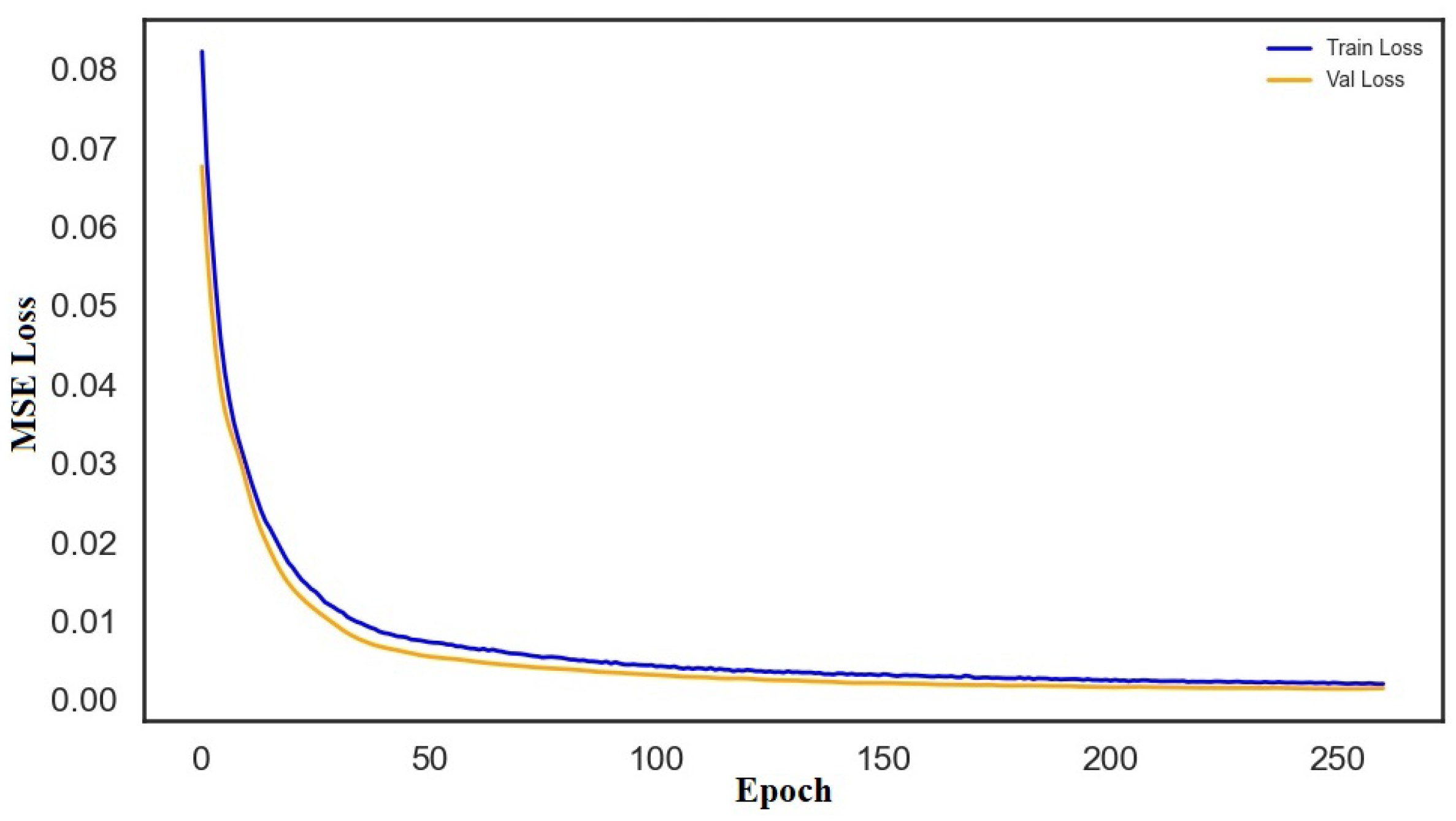
  • Learning Curve Analysis: Training and validation losses were tracked across epochs, showing that the validation loss remained stable and did not diverge notably from the training loss.

4.8. Model Evaluation Metrics

It is vital to assess the performance of ML models in predicting fragility curves. Therefore, three commonly used regression metrics, including mean square error (MSE), root mean square error (RMSE), and mean absolute percentage error (MAPE) were employed.
  • MSE: Measures the average of the squared differences between predicted and actual values; fewer values are better.
  • RMSE: As the root of MSE, it gives an interpretable error metric in the same unit as the target variable.
  • MAPE: Shows the prediction error as a percentage, making it easier to understand the accuracy of the model relative to the actual values.
These metrics offer a comprehensive view of each model’s predictive accuracy and deviation from the true outcomes [67].

5. Results and Discussion

5.1. Correlation Between Input and Output Features

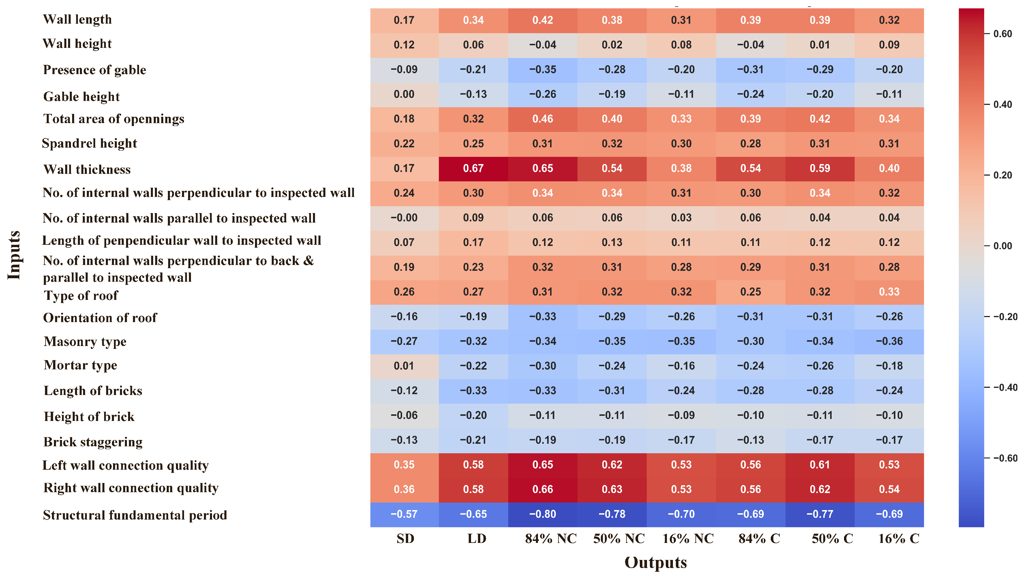
The correlation matrix, as shown in Figure 2, provides valuable and important information on the relationship between building features and the results of seismic fragility curves. It is worth noting that wall thickness and connection quality (Left Connection, Right Connection) exhibit strong positive correlations with most output variables, indicating their critical role in enhancing structural resistance during earthquakes. In contrast, the PGA exhibits a strong negative correlation with fragility thresholds, indicating that buildings with longer periods (typically more flexible) are more susceptible to seismic damage. Moderate correlations were observed for parameters such as the total opening area and the height of the story, suggesting that geometric characteristics also influence structural performance, albeit to a lesser extent. Features such as gable configuration and brick dimensions exhibit low or negligible correlations, suggesting a limited impact on fragility in this dataset. These findings help prioritize features for ML models and emphasize the importance of structural design and dynamic behavior in assessing seismic vulnerability.
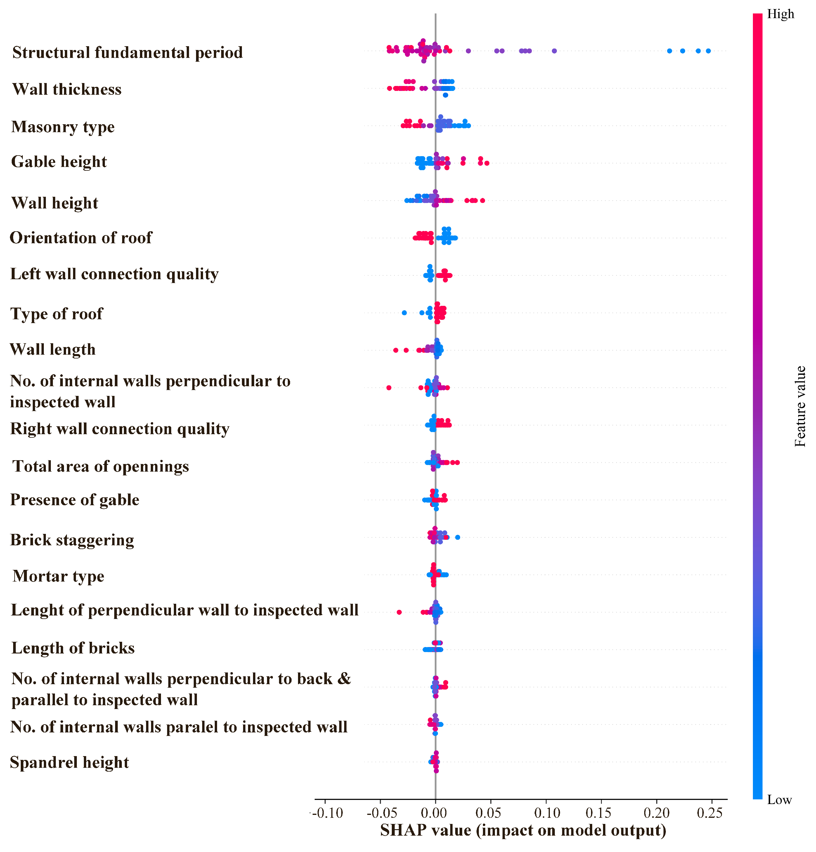
Figure 3 shows the SHAP (SHapley Additive exPlanations) values, which illustrate the relative importance and directional impact of input features on the ML models used for predicting building fragility. The results indicate that the structural fundamental period is the most influential predictor, where higher values (shown in red) are associated with positive SHAP values, thus increasing the probability of higher damage states. Similarly, wall height, masonry type, and gable height contribute strongly to the model’s output, confirming their critical role in seismic vulnerability. Features such as roof orientation, wall thickness, connection quality, and the total area of openings exhibit moderate influence, with their effects varying depending on whether the feature values are high or low. In contrast, brick dimensions, type of mortar, and roof type have minimal SHAP contributions, suggesting a limited role in driving fragility predictions. Overall, the analysis highlights that global structural and geometric parameters significantly influence the prediction process, while localized material properties have a secondary effect. This not only enhances the interpretability of the ML model but also supports targeted seismic assessment and retrofitting strategies by identifying the features most responsible for shifts in fragility curves.

5.2. Performance of ML Methods

The seven ML models, kNN, LR, SGD, DT, LSTM, XGBoost, and Transformer, were applied to the dataset, which includes field inspected buildings from Salima, Lifidzi, Golomoti, and Blantyre in Malawi.
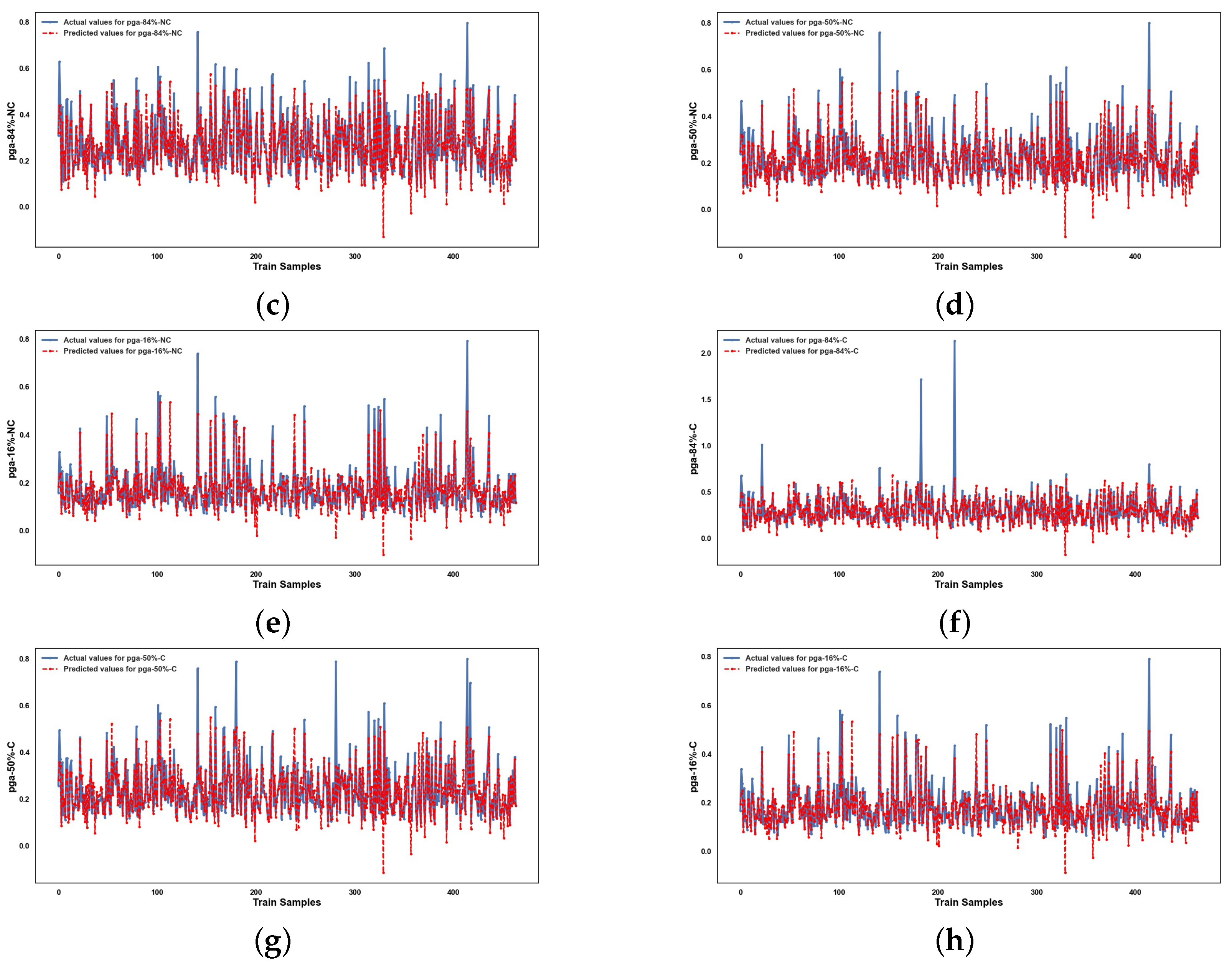
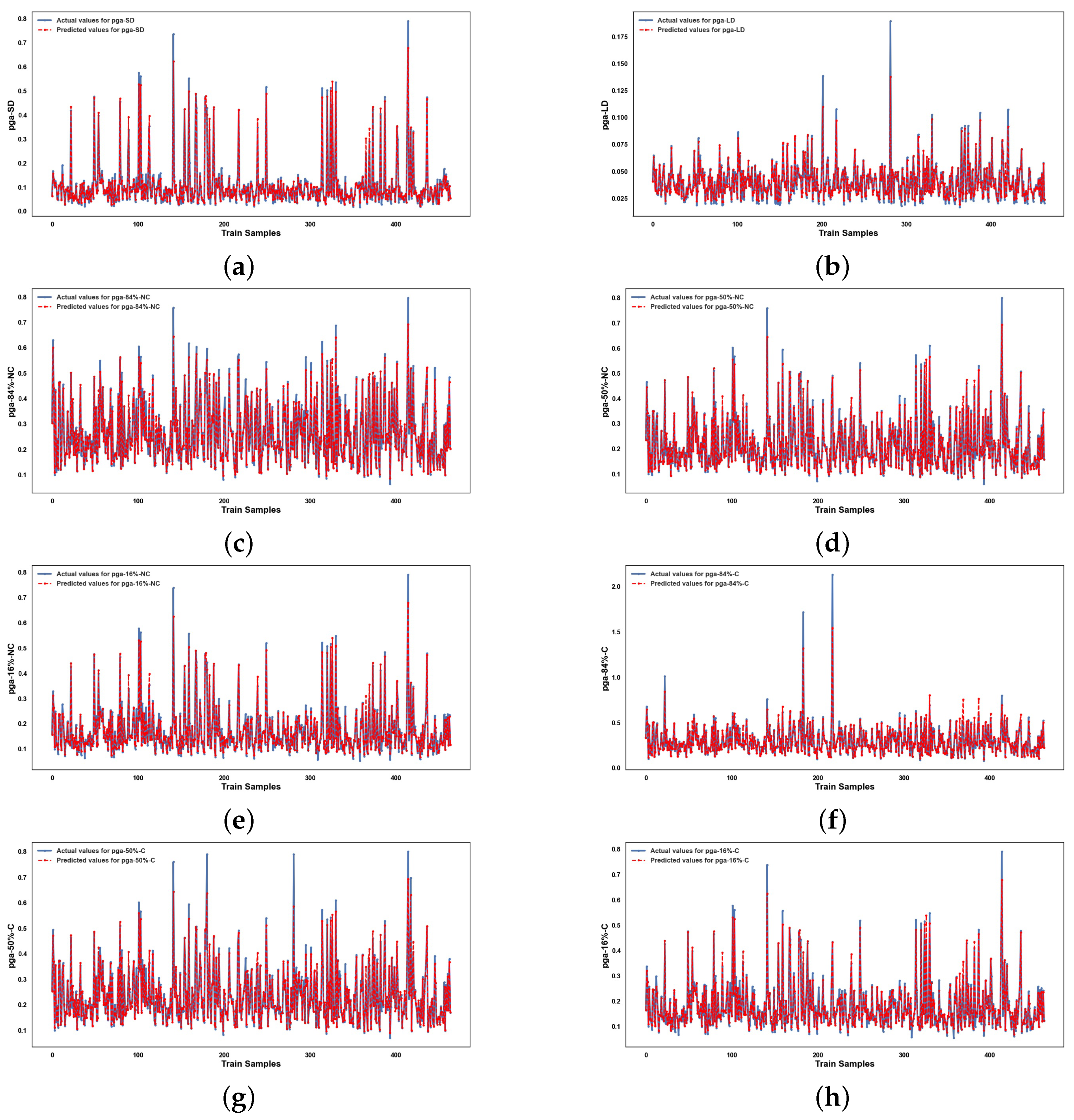
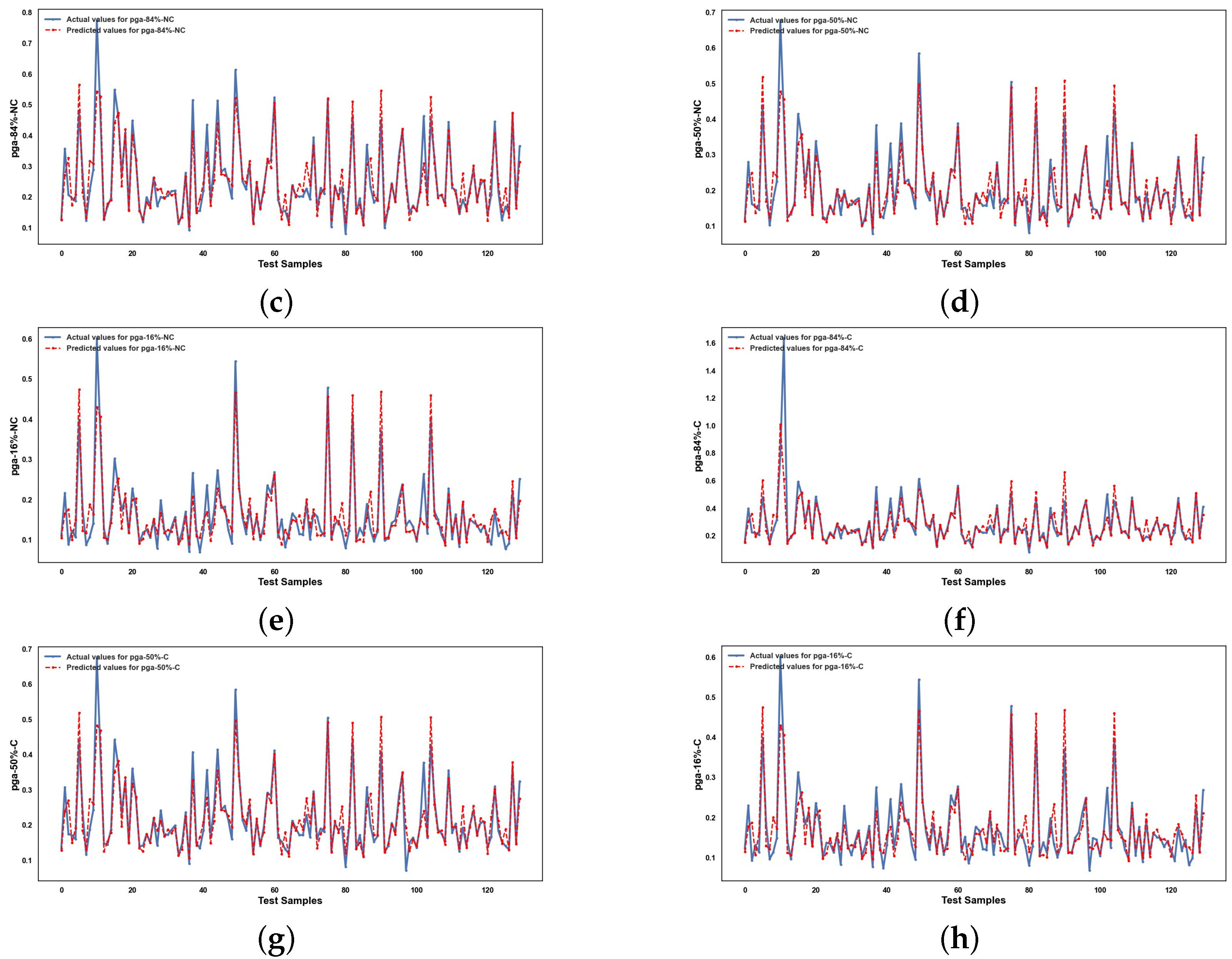
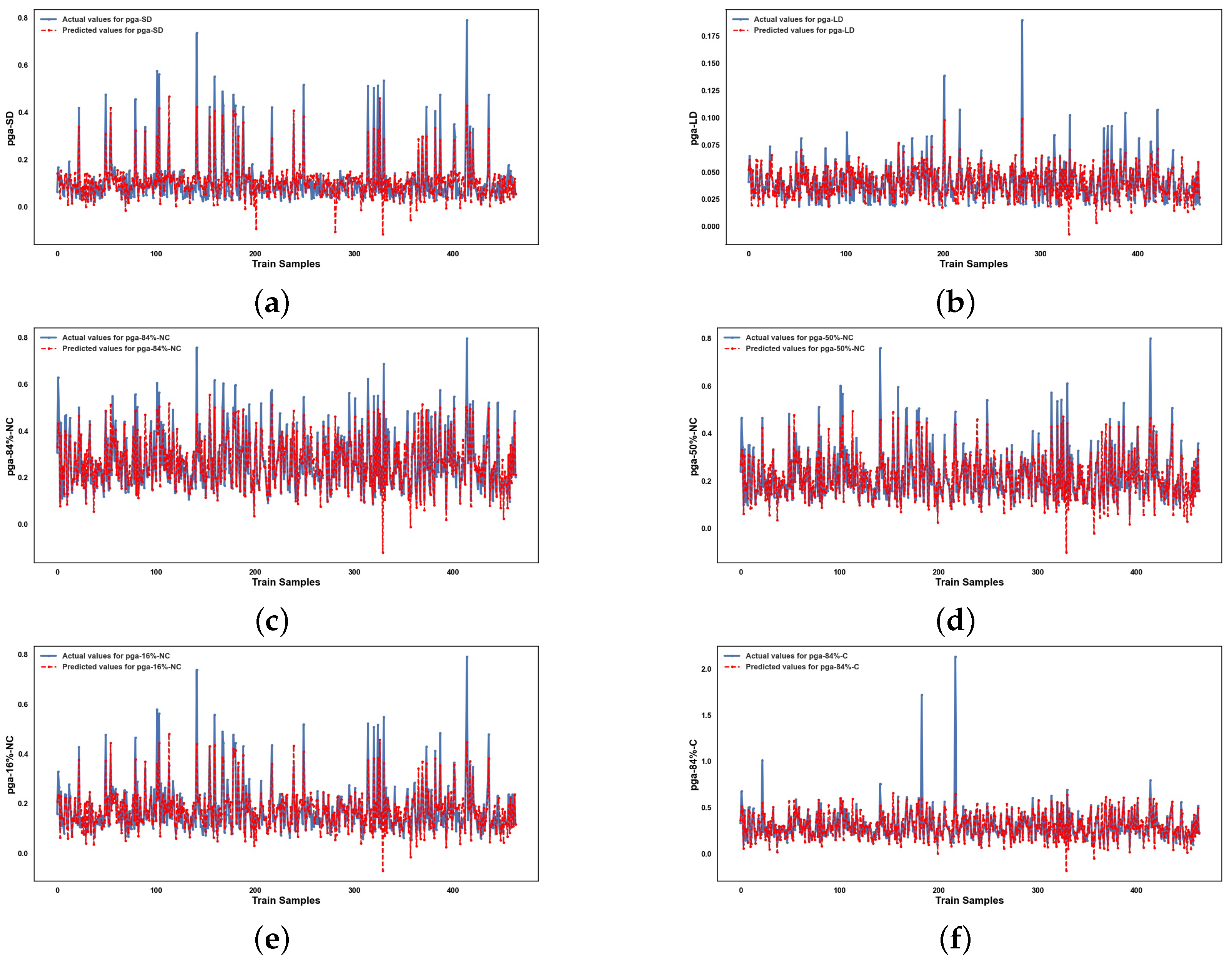
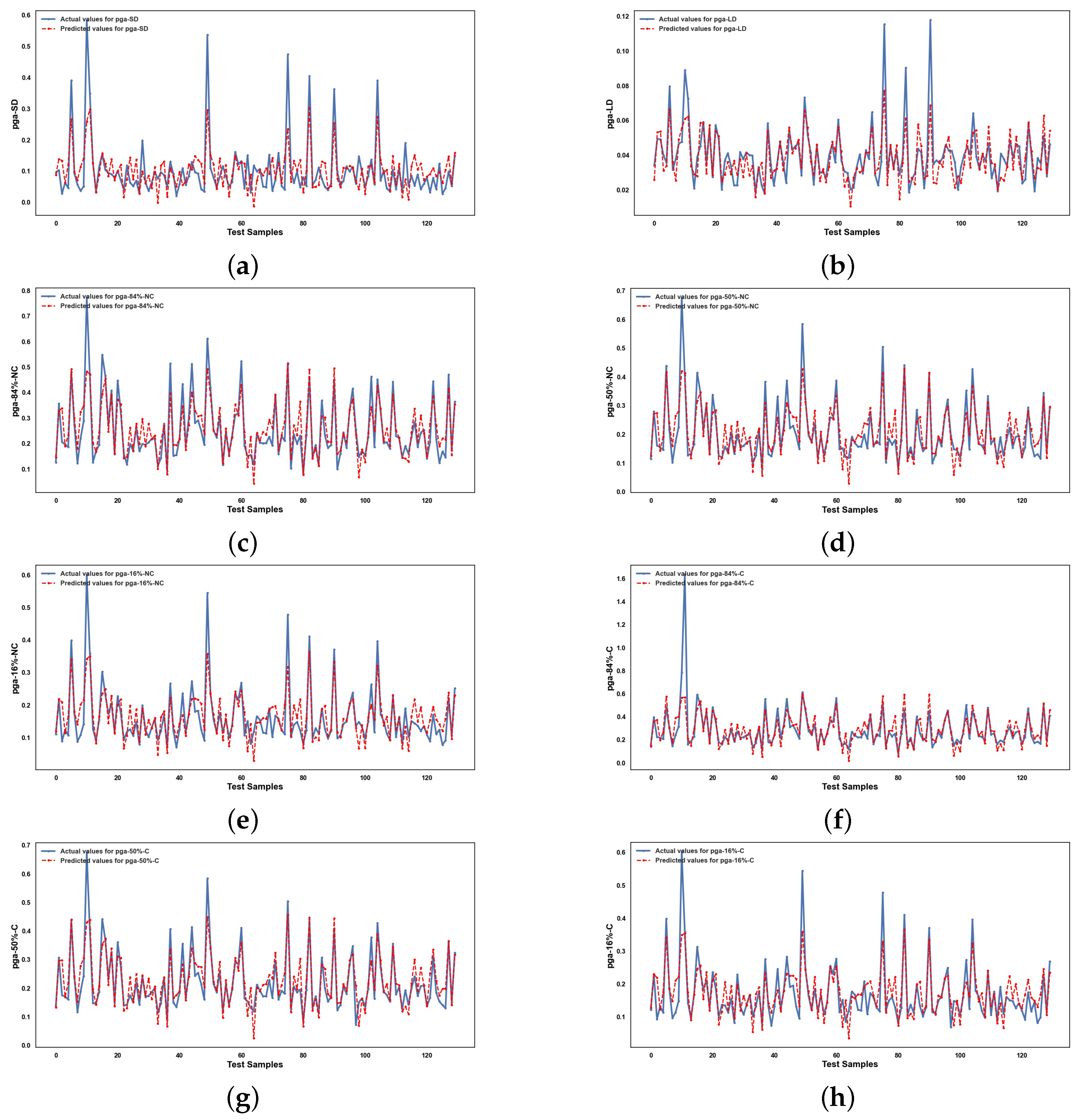
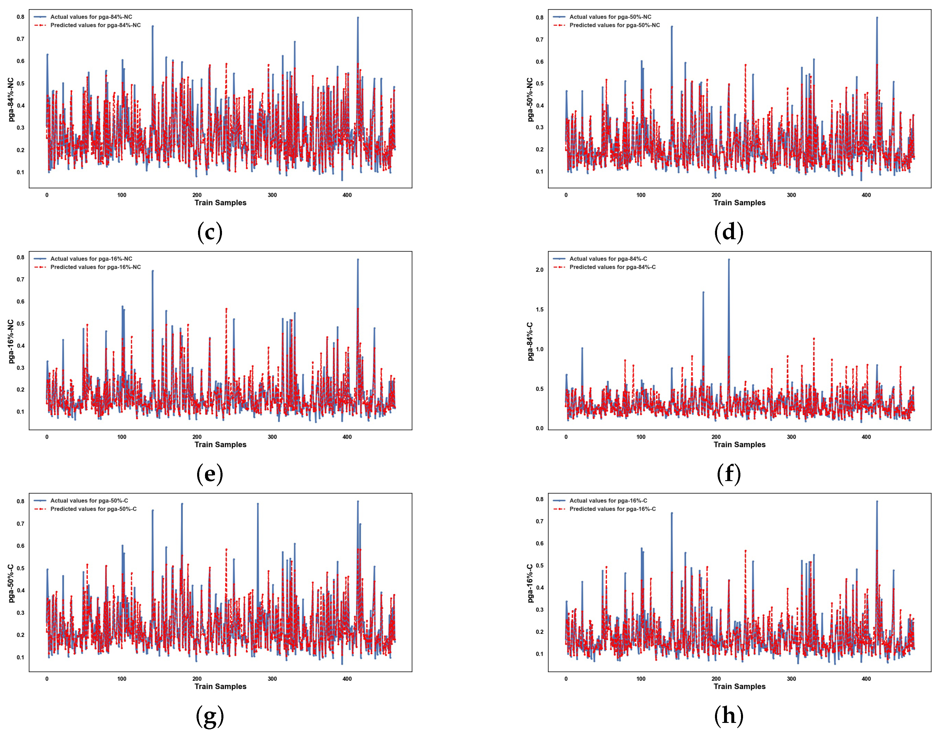
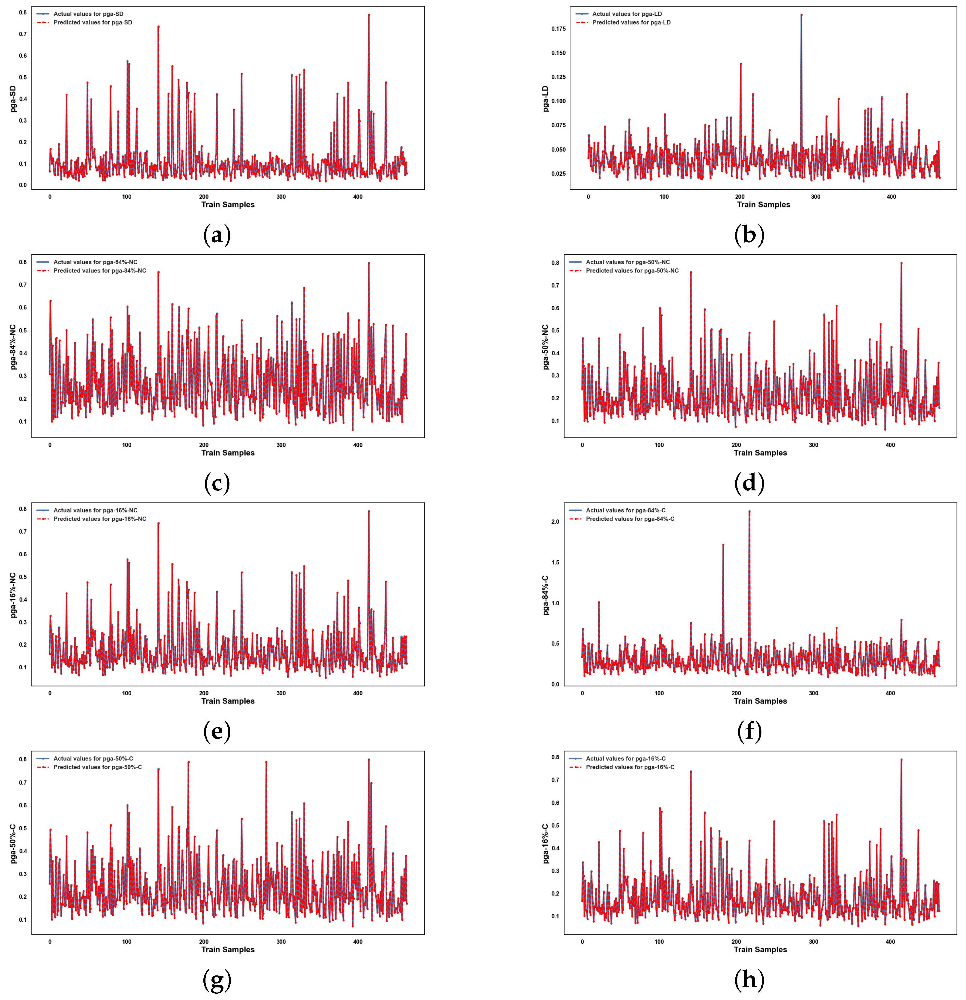
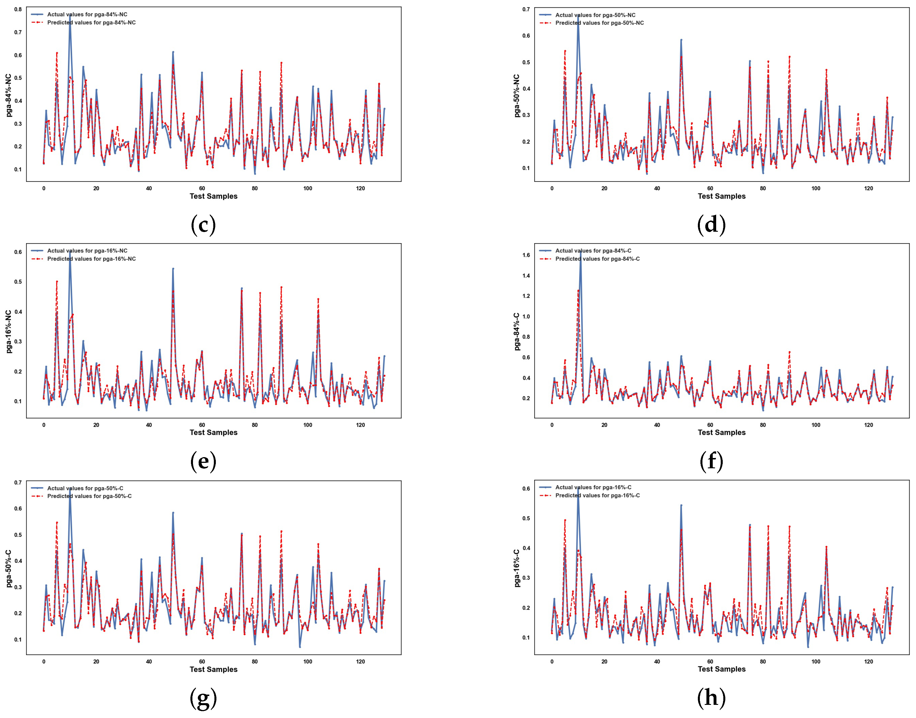
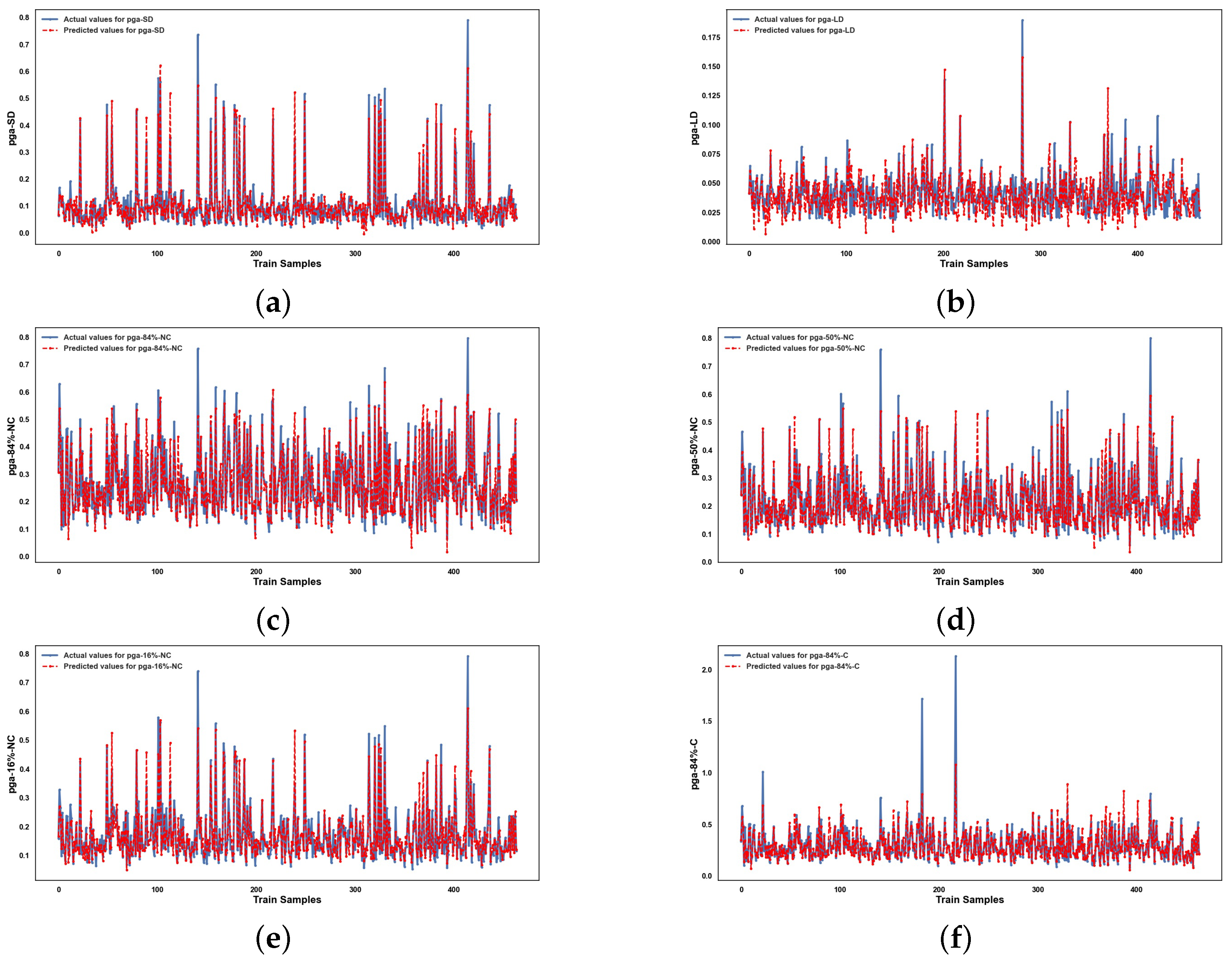
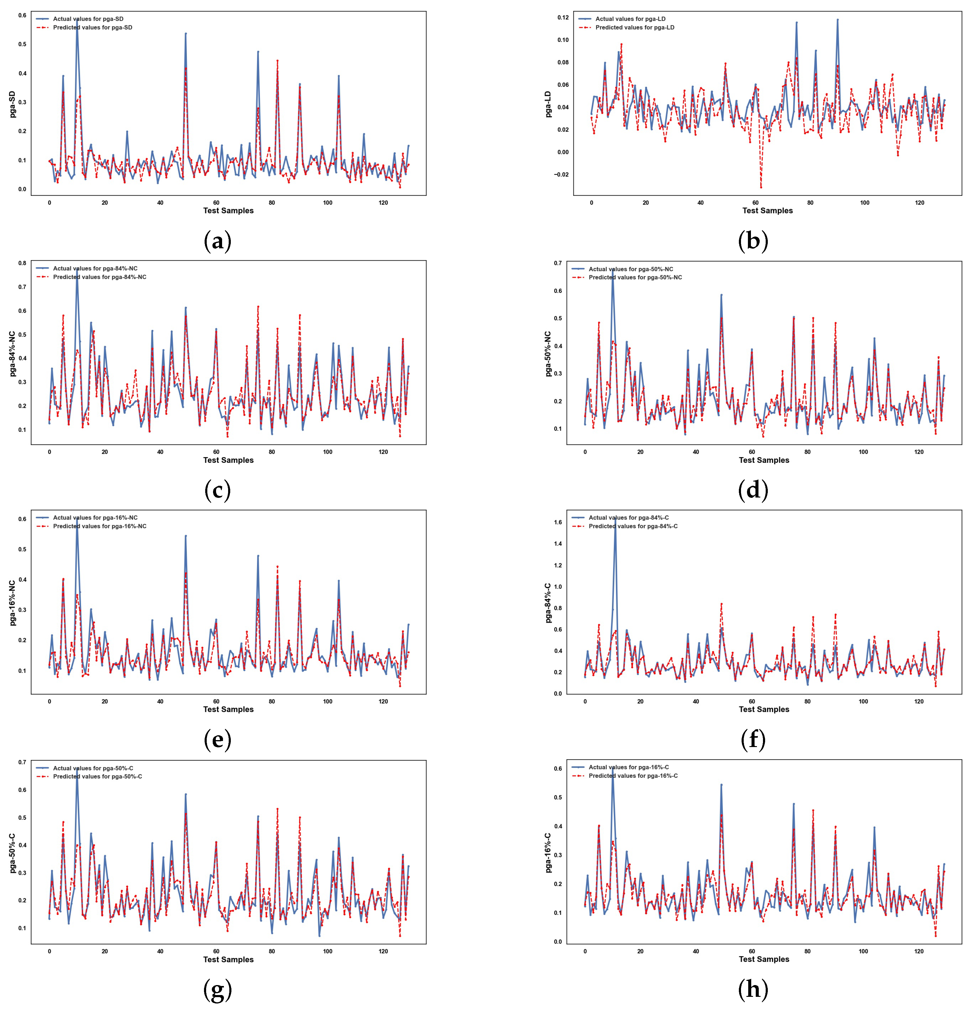
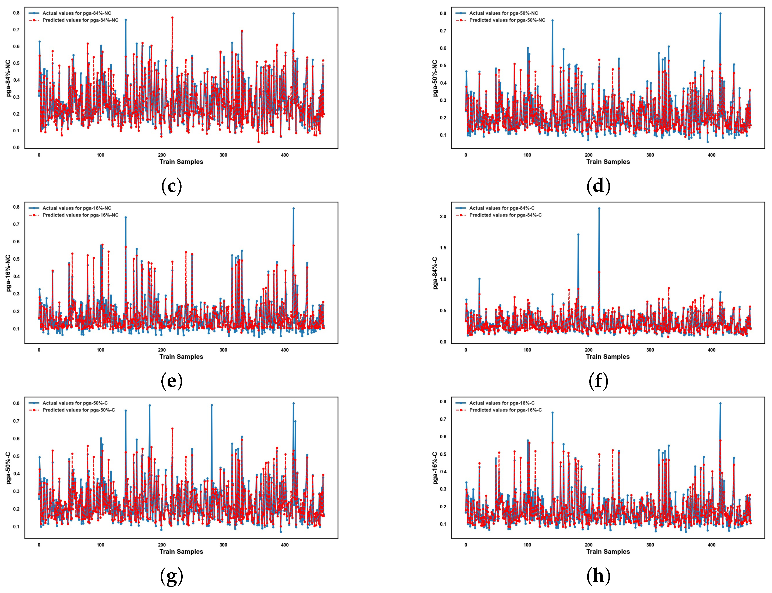
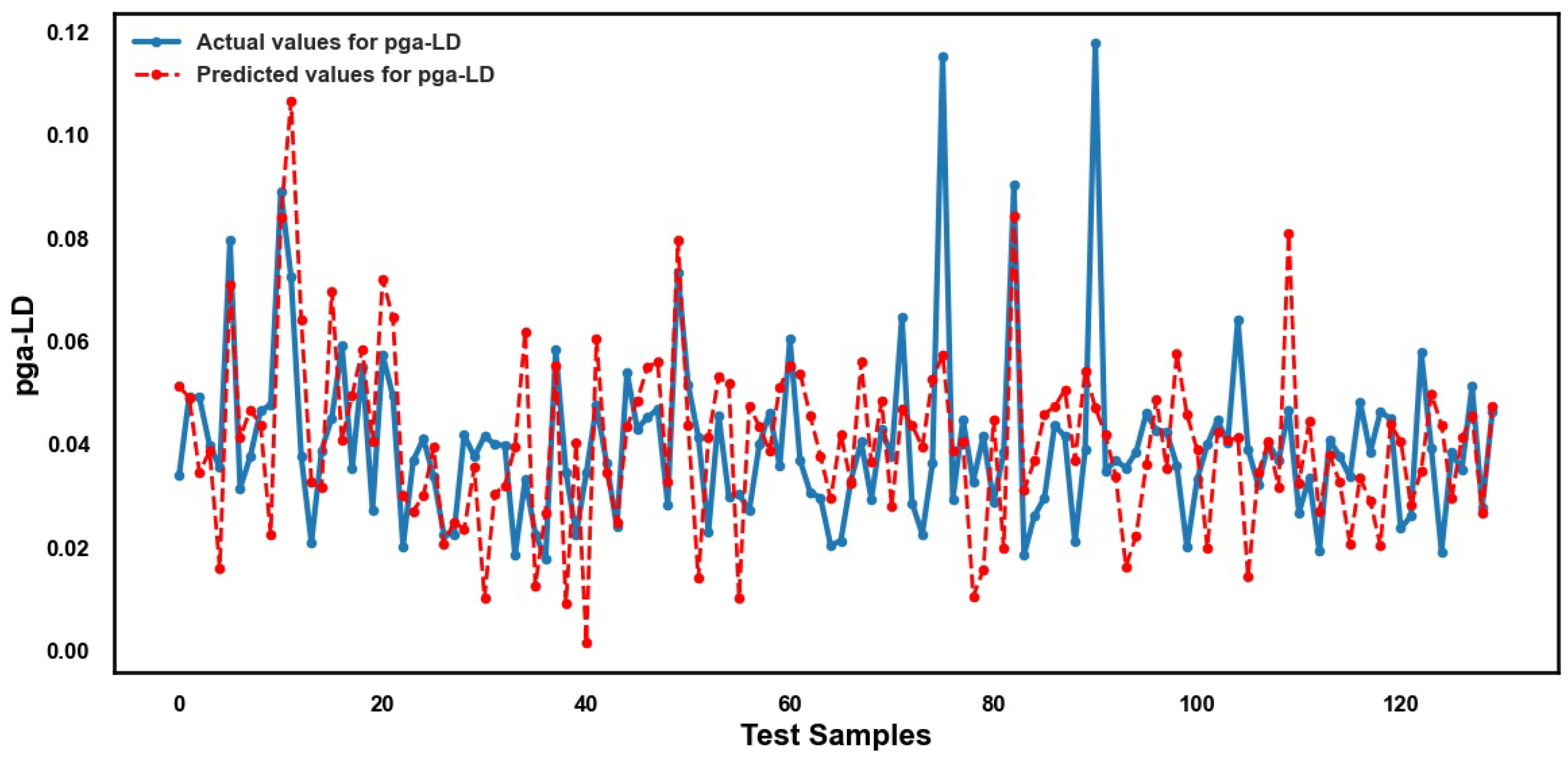
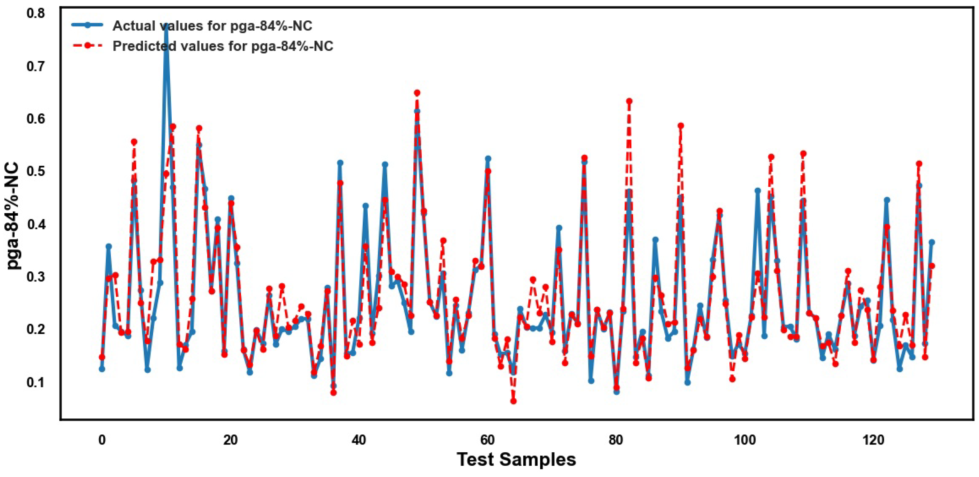
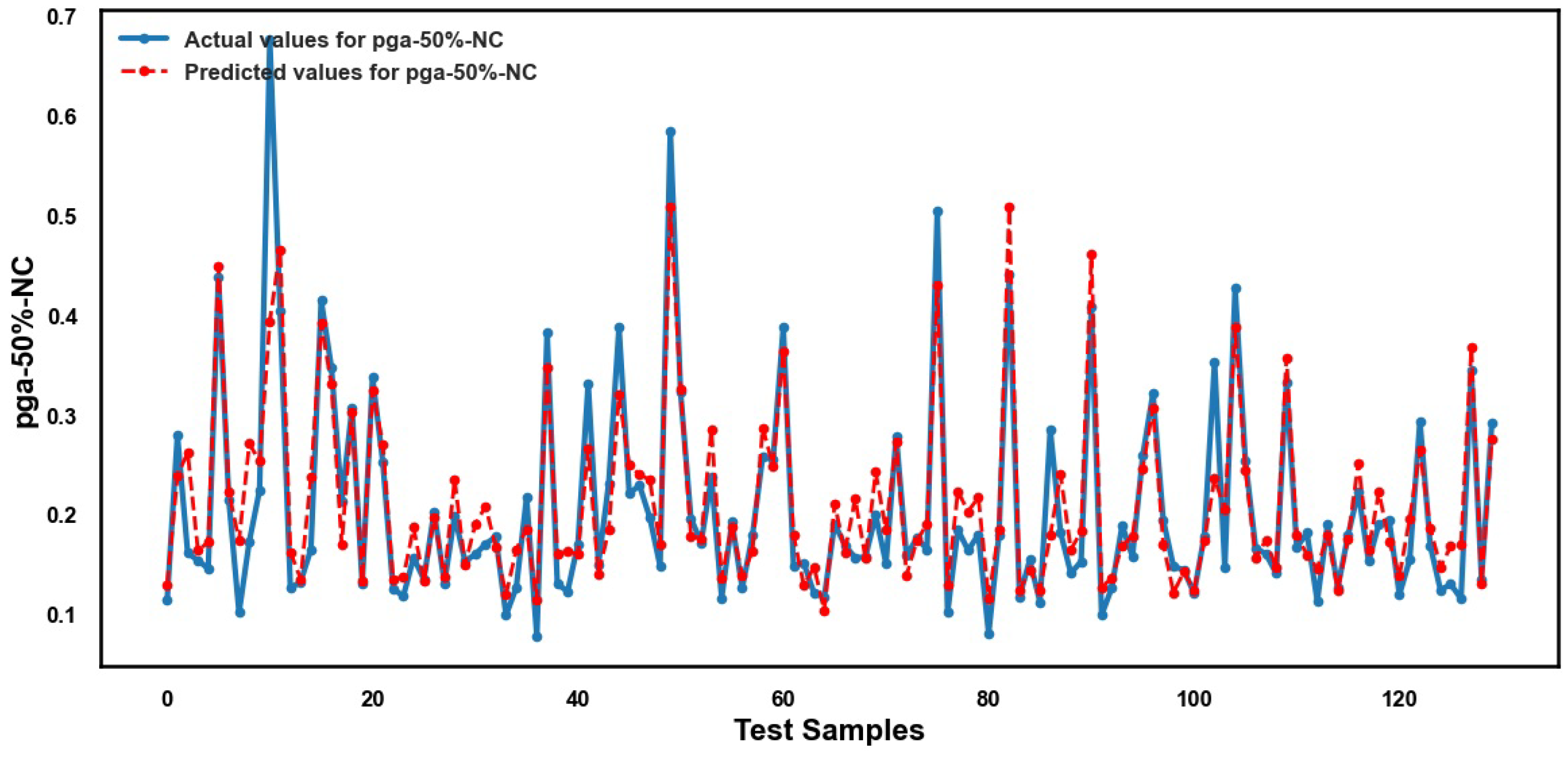
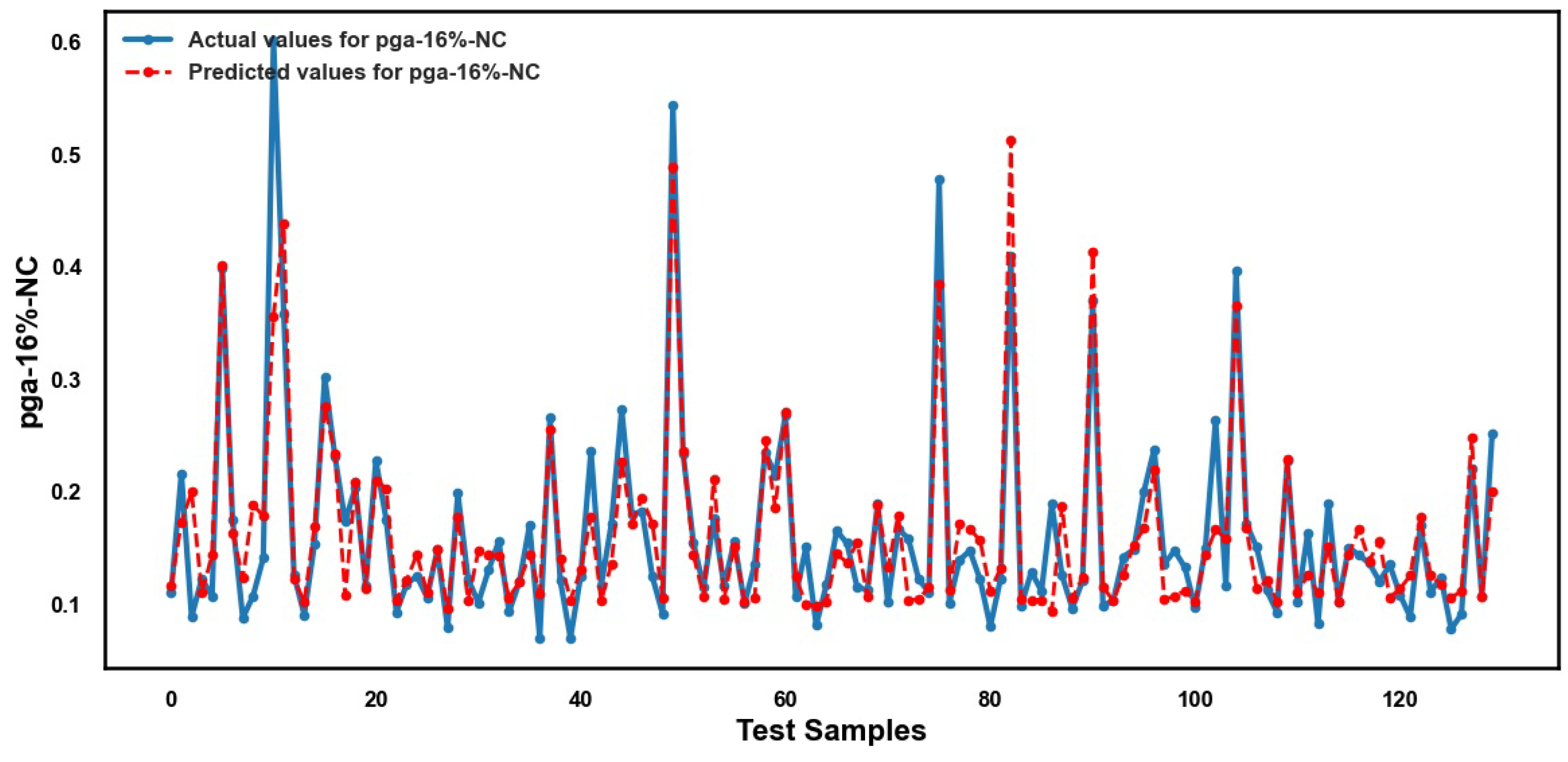
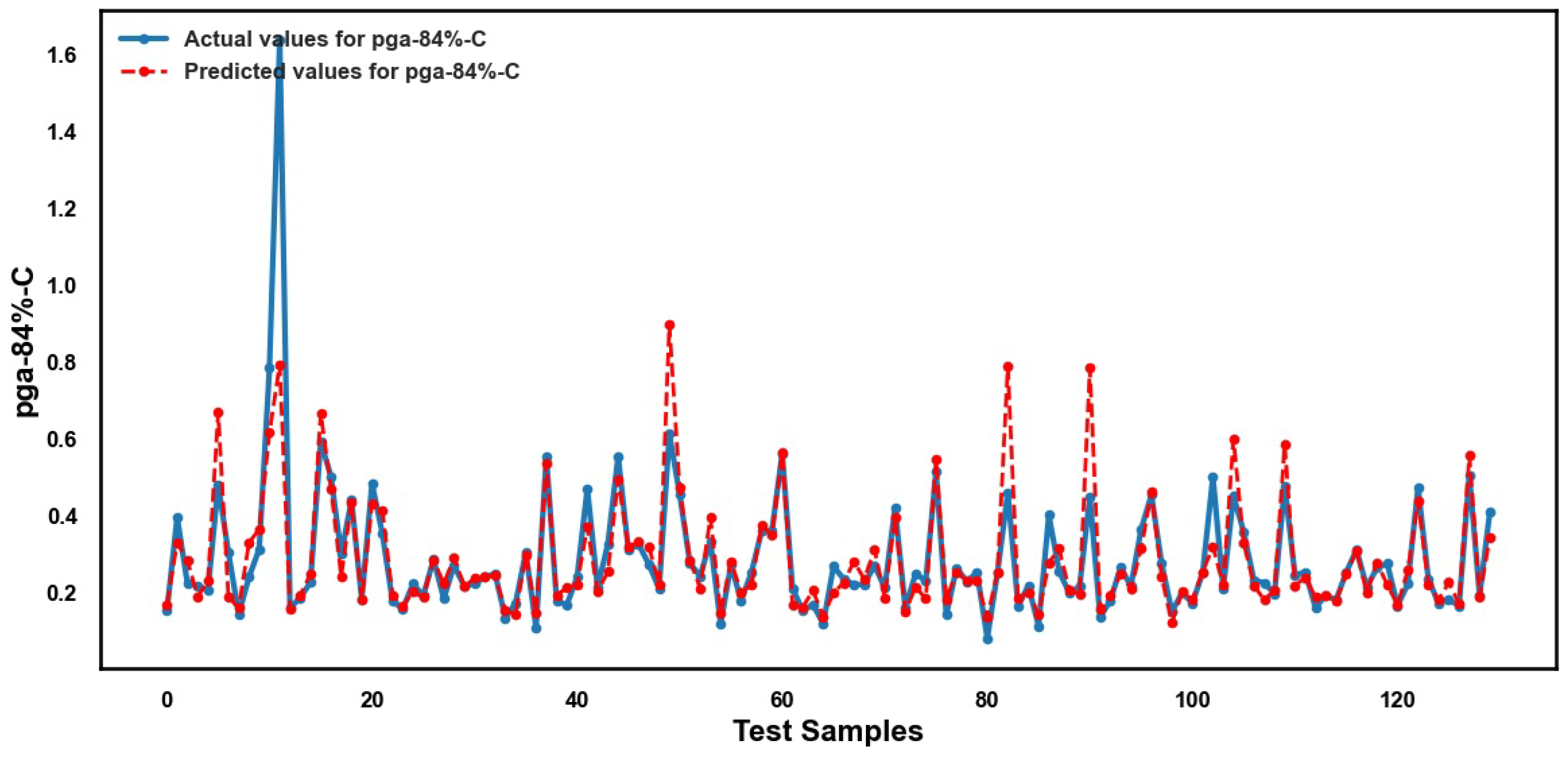
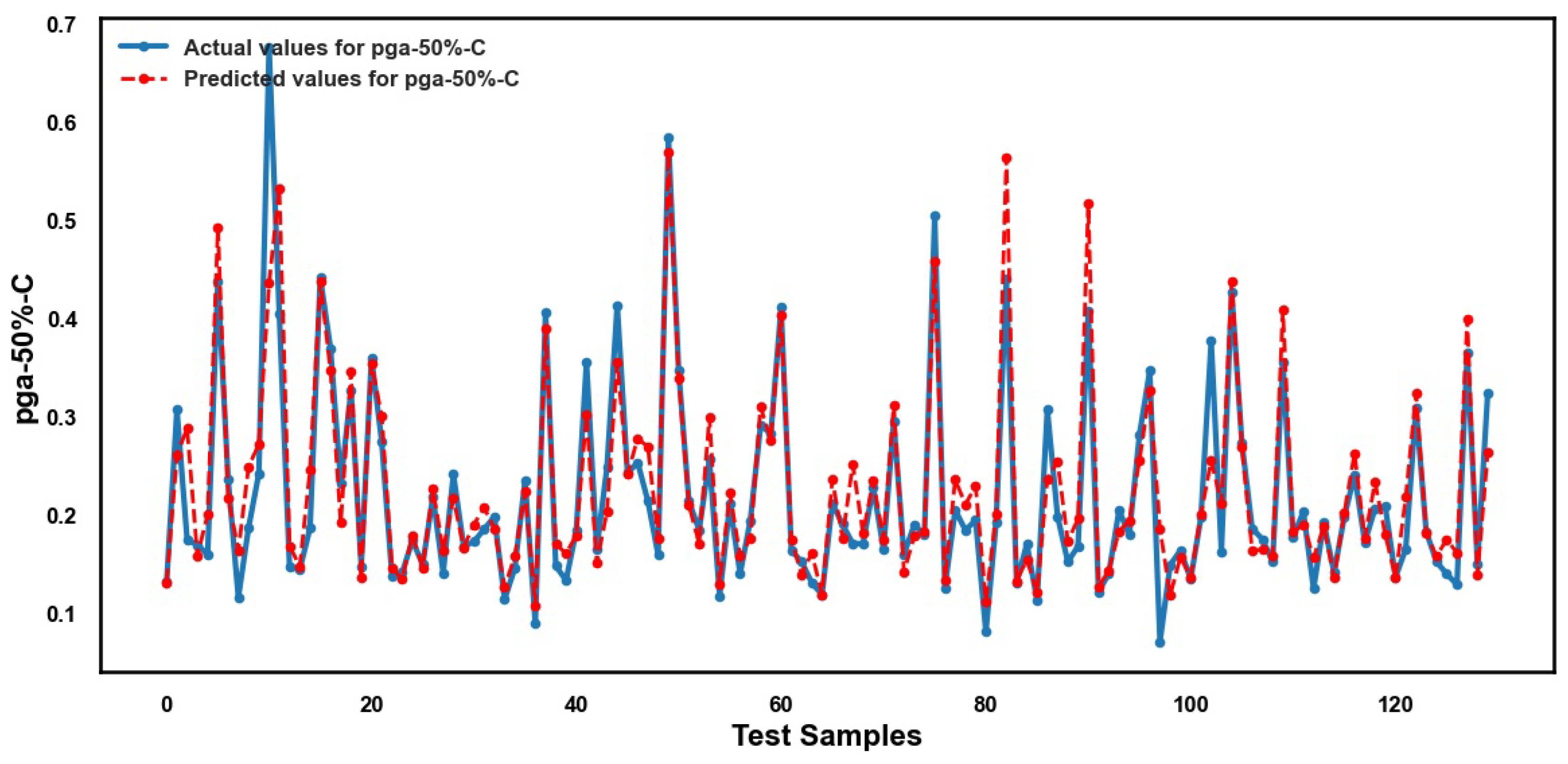
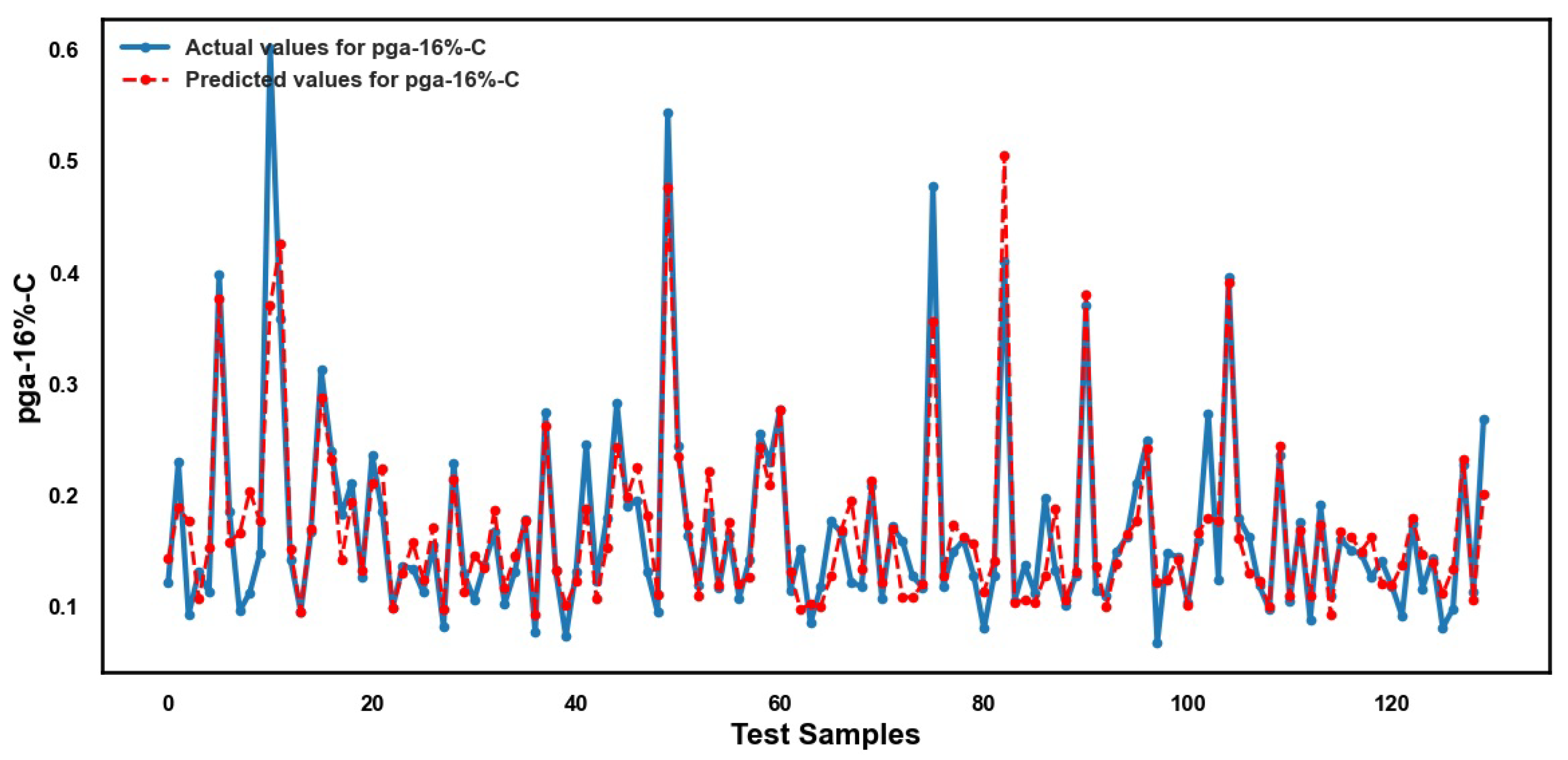
Since the primary focus of this study is on the Transformer model, and to avoid excessive visual content, only the figures for its test data predictions are shown. However, model evaluation metrics for all ML models are presented and discussed to support the analysis. Figure 4, Figure 5, Figure 6, Figure 7, Figure 8, Figure 9, Figure 10 and Figure 11 present the comparison between actual and predicted PGA (g) values in various damage states for test data using the Transformer model. The results indicate that all models demonstrated strong predictive performance, with predictions closely aligned with the observed values. To avoid an excessive number of figures for the training and testing results of different models across each damage state, the corresponding figures for each model are provided in Appendix A (Figure A1, Figure A2, Figure A3, Figure A4, Figure A5, Figure A6, Figure A7, Figure A8, Figure A9, Figure A10, Figure A11, Figure A12 and Figure A13.
Figure 12 shows the training and validation loss curves for the Transformer model over 300 Epochs, using MSE as the loss function. It can be seen that both training and validation losses decrease steadily and converge to low values. It indicates that the model effectively learned the underlying patterns in the data without overfitting. The very close alignment between the training and validation curves suggests a strong generalization to unseen data, which is essential for reliable predictions in practical applications. This kind of behavior confirms that the chosen Transformer architecture, along with the training configuration, is suitable for the regression task. Observing such a loss curve is a standard practice in model evaluation, as it provides direct insights into model performance and potential training issues such as underfitting or overfitting.
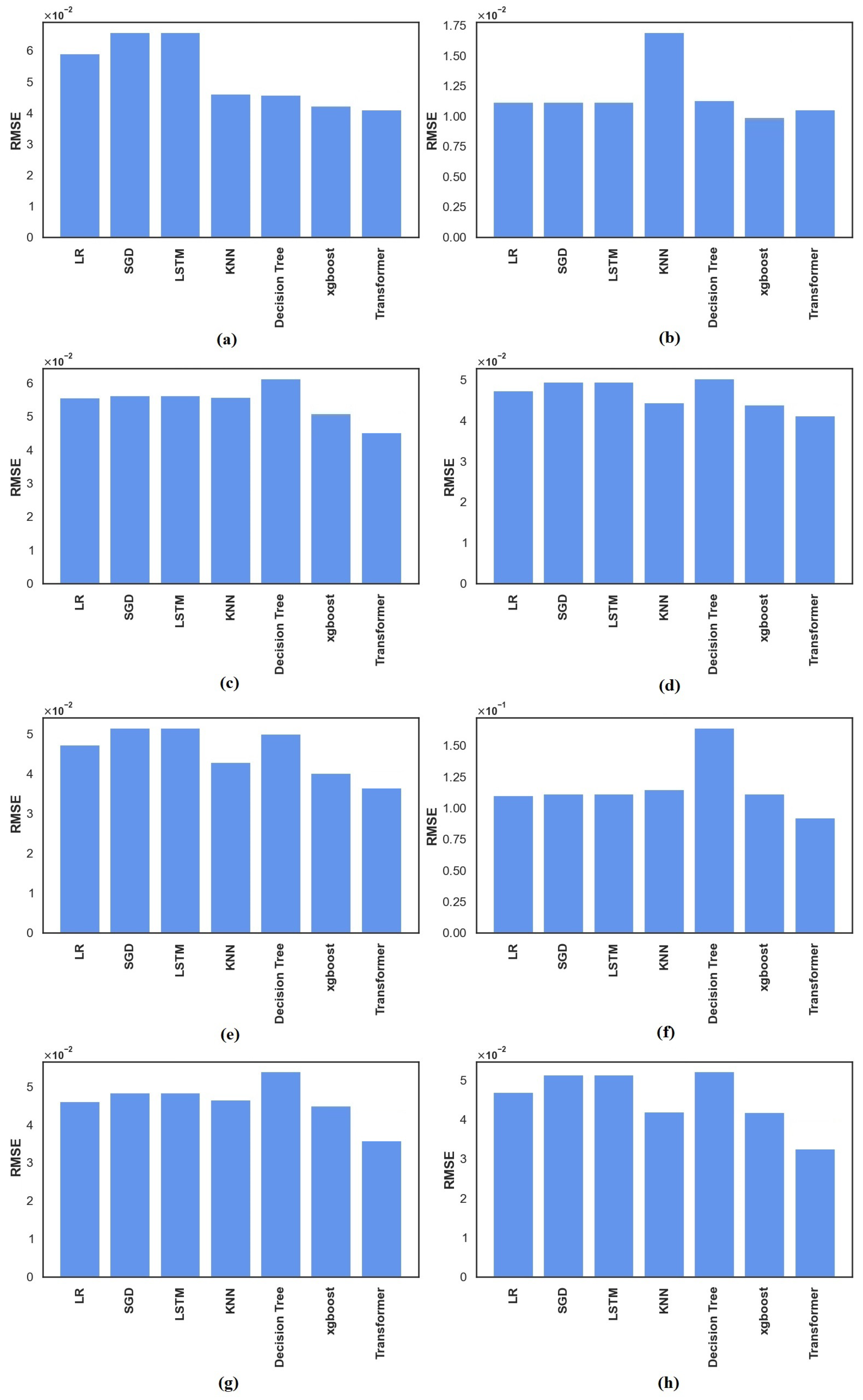
Figure 13 presents the RMSE values for each ML model at different levels of the PGA. This allows for a detailed comparison and more granular assessment of how each model behaves under varying seismic intensities.
However, given the number of combinations and the potential for visual clutter, a summarized view of the results is also provided in Figure 14, which displays the mean values of the error metrics (MAPE, RMSE, and MSE) for each model. This summary helps prevent the need for multiple separate figures, improving visual clarity and making it easier to interpret the overall performance trends of the models.
As illustrated, the Transformer model consistently achieves the lowest error values in all three metrics, indicating superior predictive accuracy and generalizability. XGBoost follows as the next best performer, showing strong predictive capability. LSTM, LR, and DT exhibit similar intermediate performances, while SGD performs slightly worse than these models in terms of MAPE and RMSE. The KNN model performs the worst, with the highest error rates, suggesting a limited predictive capacity in this context. Compared to the previous study with similar data [33], the Transformer achieved better performance, reducing the MAPE from 17.674% to 14.325% and the RMSE from 0.0617 to 0.0384. Overall, the results indicate that the Transformer model surpasses traditional ML approaches in reliably predicting PGA. Although Transformers generally perform best with large datasets, this study successfully applied the model to a relatively small dataset, demonstrating its capability to derive fragility curves effectively. This novel application highlights the feasibility of the model and its potential for broader use in future seismic vulnerability assessments. Therefore, the use of the term Strong Potential in this study emphasizes the superior predictive performance of the Transformer, as evidenced by lower MAPE and RMSE values compared to other ML models. Furthermore, the model demonstrates robust generalization across multiple output variables and effectively captures complex nonlinear relationships within seismic vulnerability data. Although training times are slightly longer and larger datasets are generally beneficial, the improved accuracy and ability of the model to model intricate interactions justify its designation as having a strong potential to derive reliable fragility curves.
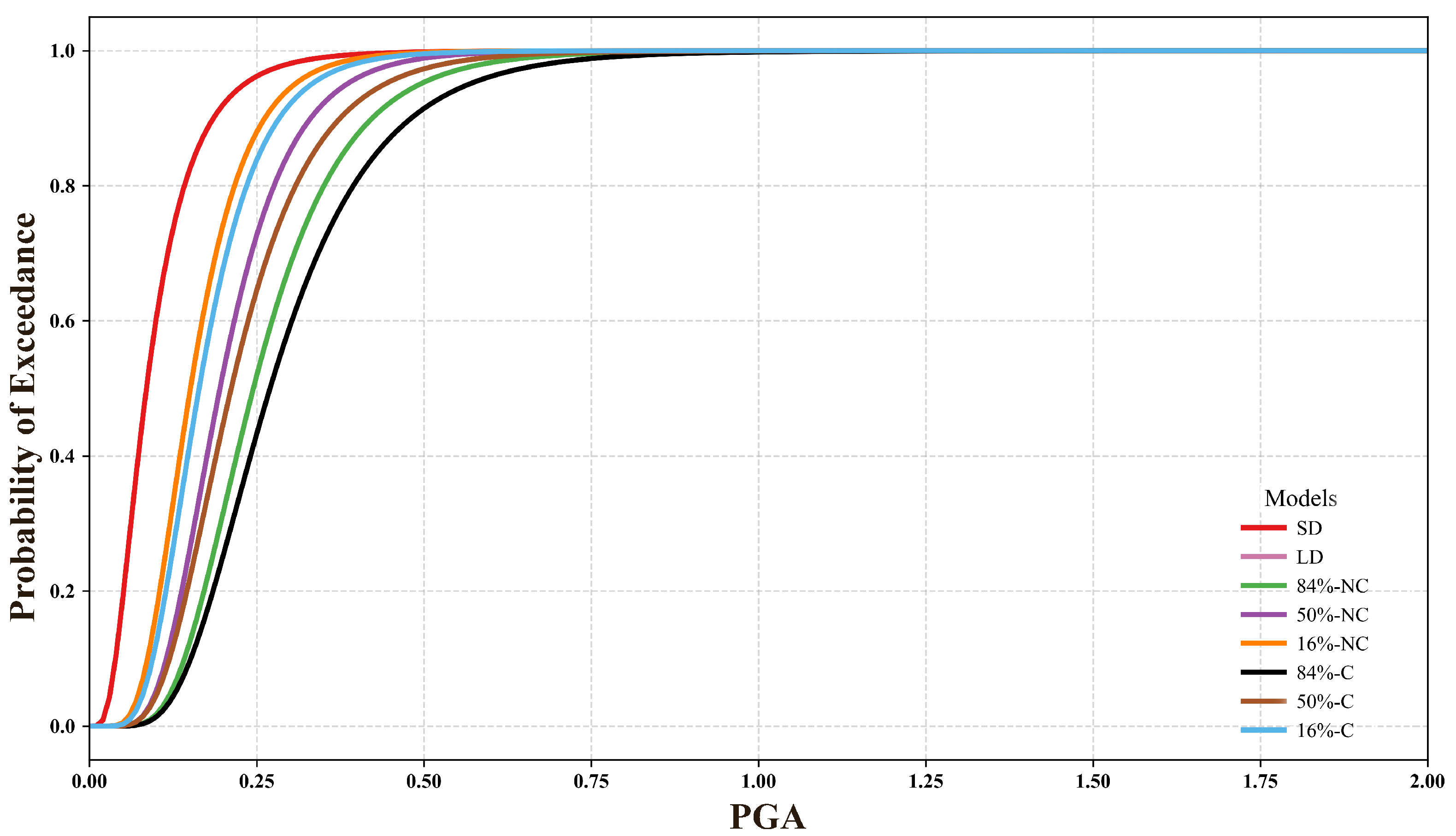
Figure 15 illustrates the fragility curves corresponding to different levels of PGA and damage states predicted by the Transformer model using the dataset. As expected, the probability of collapse increases with higher levels of PGA. The steepness and position of each curve reflect the relative vulnerability of each type of building. Buildings labeled with “SD” and “LD” exhibit the most rapid increase in the probability of collapse at lower PGA values, indicating greater fragility. In contrast, buildings classified under “C” (presumably retrofitted or reinforced) exhibit high probabilities of collapse only at higher PGA levels, particularly the 84% C curve, which shows the highest resistance. The distinction between different percentiles (16%, 50%, and 84%) further demonstrates the variability in building performance due to uncertainties in construction quality, design, and materials. In general, the figure highlights that the characteristics of the building and the structural improvements have a significant impact on the risk of collapse under seismic load.
For better comparison and visual understanding of the Transformer model’s predictions versus the actual PGA values, Figure 16 is presented. It displays the fragility curves derived from the actual dataset alongside those predicted by the Transformer model using the full dataset. As observed, the predicted PGA values closely align with the actual data, showing only minor deviations, which are slightly higher in some cases and slightly lower in others. Overall, the predictions are highly consistent and fall within an acceptable range, demonstrating the model’s reliability.

6. Conclusions

Evaluating the seismic vulnerability of non-engineered masonry buildings in developing regions is crucial for minimizing risk to life and property in earthquake-prone areas. These buildings often lack structural resilience, making them especially susceptible to damage during seismic events. Given the extensive losses observed in past earthquakes, there is a growing need for data-driven strategies to support effective retrofitting and mitigation efforts. With the advancement of ML, new opportunities have emerged for seismic risk assessment. In this study, seven algorithms (kNN, LR, SGD, DT, LSTM, XGBoost, and Transformer) were trained on field-collected data from 646 masonry walls in Malawi to estimate collapse probabilities and derive fragility curves.
Among all models, the Transformer achieved the best performance, producing fragility curves that closely matched empirical data (Figure 16). Its capacity to capture complex nonlinear relationships distinguished it from the more conventional algorithms. Overall, the results demonstrate that Transformer-based models are a promising tool for assessing seismic fragility in non-engineered buildings. Their predictive accuracy and consistency with observed trends support their potential for real-world application and broader deployment.
Although the dataset was limited to Malawi, the findings are broadly representative of East African non-engineered masonry, where materials and construction practices are comparable. Laboratory testing of local materials increased confidence in the fragility curves, ensuring they capture regional structural behavior.
Future work could improve prediction performance by expanding datasets (more surveyed buildings and seismic records), testing alternative ML models, and integrating additional structural and environmental features relevant to target regions. These directions will strengthen model robustness and advance data-driven approaches for seismic vulnerability assessment.

Author Contributions

Conceptualization, E.H. and V.I.N.; methodology, E.H.; software, E.H.; validation, E.H. and V.I.N.; formal analysis, E.H.; investigation, E.H.; resources, V.I.N.; data curation, V.I.N.; writing—original draft preparation, E.H. and V.I.N.; writing—review and editing, E.H. and V.I.N.; visualization, E.H.; supervision, E.H.; project administration, E.H.; funding acquisition, E.H. All authors have read and agreed to the published version of the manuscript.

Funding

This research received no external funding.

Data Availability Statement

Data will be made available on request.

Conflicts of Interest

The authors declare no conflicts of interest.

Abbreviations

The following abbreviations are used in this manuscript:
ANNArtificial Neural Network
CCollapse
DTDecision Tree
IDAIncremental Dynamic Analysis
KNNK-Nearest Neighbors
LDLight Damage
LRLinear Regression
LSTMLong Short-Term Memory
MAPEMean Absolute Percentage Error
MLMachine Learning
MSEMean Squared Error
NCNear Collapse
PGAPeak Ground Acceleration
RMSERoot Mean Square Error
SDSevere Damage
SGDStochastic Gradient Descent
SHAPSHapley Additive exPlanations
SPOStatic Pushover
XGBoostExtreme Gradient Boosting

Appendix A

Figure A1. Actual and predicted values obtained from the LR model for the training dataset: (a) SD, (b) LD, (c) 84% NC, (d) 50% NC, (e) 16% NC, (f) 84% C, (g) 50% C, and (h) 16% C.
Infrastructures 10 00279 g0a1aInfrastructures 10 00279 g0a1b
Figure A2. Actual and predicted values obtained from the LR model for the test dataset: (a) SD, (b) LD, (c) 84% NC, (d) 50% NC, (e) 16% NC, (f) 84% C, (g) 50% C, and (h) 16% C.
Infrastructures 10 00279 g0a2aInfrastructures 10 00279 g0a2b
Figure A3. Actual and predicted values obtained from the RF model for the training dataset: (a) SD, (b) LD, (c) 84% NC, (d) 50% NC, (e) 16% NC, (f) 84% C, (g) 50% C, and (h) 16% C.
Infrastructures 10 00279 g0a3
Figure A4. Actual and predicted values obtained from the RF model for the test dataset: (a) SD, (b) LD, (c) 84% NC, (d) 50% NC, (e) 16% NC, (f) 84% C, (g) 50% C, and (h) 16% C.
Infrastructures 10 00279 g0a4aInfrastructures 10 00279 g0a4b
Figure A5. Actual and predicted values obtained from the SGD model for the training dataset: (a) SD, (b) LD, (c) 84% NC, (d) 50% NC, (e) 16% NC, (f) 84% C, (g) 50% C, and (h) 16% C.
Infrastructures 10 00279 g0a5aInfrastructures 10 00279 g0a5b
Figure A6. Actual and predicted values obtained from the SGD model for the test dataset: (a) SD, (b) LD, (c) 84% NC, (d) 50% NC, (e) 16% NC, (f) 84% C, (g) 50% C, and (h) 16% C.
Infrastructures 10 00279 g0a6
Figure A7. Actual and predicted values obtained from the KNN model for the training dataset: (a) SD, (b) LD, (c) 84% NC, (d) 50% NC, (e) 16% NC, (f) 84% C, (g) 50% C, and (h) 16% C.
Infrastructures 10 00279 g0a7aInfrastructures 10 00279 g0a7b
Figure A8. Actual and predicted values obtained from the KNN model for the test dataset: (a) SD, (b) LD, (c) 84% NC, (d) 50% NC, (e) 16% NC, (f) 84% C, (g) 50% C, and (h) 16% C.
Infrastructures 10 00279 g0a8aInfrastructures 10 00279 g0a8b
Figure A9. Actual and predicted values obtained from the XGBoost model for the training dataset: (a) SD, (b) LD, (c) 84% NC, (d) 50% NC, (e) 16% NC, (f) 84% C, (g) 50% C, and (h) 16% C.
Infrastructures 10 00279 g0a9
Figure A10. Actual and predicted values obtained from the XGBoost model for the test dataset: (a) SD, (b) LD, (c) 84% NC, (d) 50% NC, (e) 16% NC, (f) 84% C, (g) 50% C, and (h) 16% C.
Infrastructures 10 00279 g0a10aInfrastructures 10 00279 g0a10b
Figure A11. Actual and predicted values obtained from the LSTM model for the training dataset: (a) SD, (b) LD, (c) 84% NC, (d) 50% NC, (e) 16% NC, (f) 84% C, (g) 50% C, and (h) 16% C.
Infrastructures 10 00279 g0a11aInfrastructures 10 00279 g0a11b
Figure A12. Actual and predicted values obtained from the LSTM model for the test dataset: (a) SD, (b) LD, (c) 84% NC, (d) 50% NC, (e) 16% NC, (f) 84% C, (g) 50% C, and (h) 16% C.
Infrastructures 10 00279 g0a12
Figure A13. Actual and predicted values obtained from the Transformer model for the training dataset: (a) SD, (b) LD, (c) 84% NC, (d) 50% NC, (e) 16% NC, (f) 84% C, (g) 50% C, and (h) 16% C.
Infrastructures 10 00279 g0a13aInfrastructures 10 00279 g0a13b

References

  1. Bazzurro, P.; Cornell, C.; Menun, C.; Motahari, M. Guidelines for seismic assessment of damaged buildings. In Proceedings of the 13th World Conference on Earthquake Engineering, Vancouver, BC, Canada, 1–6 August 2004; Volume 1708. [Google Scholar]
  2. Nirandjan, S.; Koks, E.E.; Ye, M.; Pant, R.; Van Ginkel, K.C.; Aerts, J.C.; Ward, P.J. Physical vulnerability database for critical infrastructure multi-hazard risk assessments–A systematic review and data collection. Nat. Hazards Earth Syst. Sci. Discuss. 2024, 24, 4341–4368. [Google Scholar] [CrossRef]
  3. Rota, M.; Penna, A.; Strobbia, C. Processing Italian damage data to derive typological fragility curves. Soil Dyn. Earthq. Eng. 2008, 28, 933–947. [Google Scholar] [CrossRef]
  4. Yepes-Estrada, C.; Silva, V.; Crowley, H. Gem vulnerability database for the openquake-platform. In Proceedings of the Second European Conference on Earthquake Engineering and Seismology, Istanbul, Turkey, 25–29 August 2014. [Google Scholar]
  5. Di Ludovico, M.; De Martino, G.; Prota, A.; Manfredi, G.; Dolce, M. Relationships between empirical damage and direct/indirect costs for the assessment of seismic loss scenarios. Bull. Earthq. Eng. 2022, 20, 229–254. [Google Scholar] [CrossRef]
  6. Ahmad, S.; Kyriakides, N.; Pilakoutas, K.; Neocleous, K.; Zaman, Q.U. Seismic fragility assessment of existing sub-standard low strength reinforced concrete structures. Earthq. Eng. Eng. Vib. 2015, 14, 439–452. [Google Scholar] [CrossRef]
  7. Khalfan, M.; El-Dakhakhni, W.W.; Tait, M.J. Seismic risk assessment of nonengineered residential buildings in developing countries. J. Perform. Constr. Facil. 2016, 30, 4016013. [Google Scholar] [CrossRef]
  8. Novelli, V.; Risi, R.; Ngoma, I.; Kafodya, I.; Kloukinas, P.; Macdonald, J.; Goda, K. Fragility curves for non-engineered masonry buildings in developing countries derived from real data based on structural surveys and laboratory tests. Soft Comput. 2021, 25, 6113–6138. [Google Scholar] [CrossRef]
  9. Khalfan, M. Fragility Curves for Residential Buildings in Developing Countries: A Case Study on Non-Engineered Unreinforced Masonry Homes in Bantul, Indonesia. Master’s Thesis, McMaster University, Hamilton, ON, Canada, 2013. [Google Scholar]
  10. Dai, K.Y.; Yu, X.H.; Lu, D.G.; Qian, K. Fragility functions for corroded reinforced concrete columns. J. Build. Eng. 2024, 82, 108124. [Google Scholar] [CrossRef]
  11. Yu, X.; Li, Z.; Yang, A.; Li, Y.; Lu, D.; Dai, K. Time-Dependent Seismic Fragility of Coastal RC Frames Considering Effect of Distance from Coastline. Buildings 2025, 15, 737. [Google Scholar] [CrossRef]
  12. Sabetta, F.; Goretti, A.; Lucantoni, A. Empirical fragility curves from damage surveys and estimated strong ground motion. In Proceedings of the 11th European Conference on Earthquake Engineering, Paris, France, 6–11 September 1998; pp. 1–11. [Google Scholar]
  13. Du, A.; Wang, X.; Xie, Y.; Dong, Y. Regional seismic risk and resilience assessment: Methodological development, applicability, and future research needs–An earthquake engineering perspective. Reliab. Eng. Syst. Saf. 2023, 233, 109104. [Google Scholar] [CrossRef]
  14. Guo, J.; Zhang, P.; Wang, J.; Li, S.; Guan, Z. A novel framework for seismic fragility analysis with the combination of Box-Cox transformation and Bayesian inference. Eng. Struct. 2023, 277, 115436. [Google Scholar] [CrossRef]
  15. Işık, E.; Bilgin, H.; Avcil, F.; İzol, R.; Arkan, E.; Büyüksaraç, A.; Harirchian, E.; Hysenlliu, M. Seismic performances of masonry educational buildings during the 2023 Türkiye (Kahramanmaraş) Earthquakes. GeoHazards 2024, 5, 700–731. [Google Scholar] [CrossRef]
  16. Giordano, N.; De Risi, R.; Voyagaki, E.; Kloukinas, P.; Novelli, V.; Kafodya, I.; Ngoma, I.; Goda, K.; Macdonald, J. Seismic fragility models for typical non-engineered URM residential buildings in Malawi. Structures 2021, 32, 2266–2278. [Google Scholar] [CrossRef]
  17. Harirchian, E.; Hosseini, S.E.A.; Jadhav, K.; Kumari, V.; Rasulzade, S.; Işık, E.; Wasif, M.; Lahmer, T. A review on application of soft computing techniques for the rapid visual safety evaluation and damage classification of existing buildings. J. Build. Eng. 2021, 43, 102536. [Google Scholar] [CrossRef]
  18. Dabiri, H.; Faramarzi, A.; Dall’Asta, A.; Tondi, E.; Micozzi, F. A machine learning-based analysis for predicting fragility curve parameters of buildings. J. Build. Eng. 2022, 62, 105367. [Google Scholar] [CrossRef]
  19. Thedy, J.; Liao, K.W. Machine Learning-Enhanced Fragility Curves: Advancing Reliability and Safety of Structures in Seismic Risk Assessment. Reliab. Eng. Syst. Saf. 2025, 264, 111361. [Google Scholar] [CrossRef]
  20. Rajapaksha, R.; Siriwardana, C. A systematic review on different approaches used in the development of fragility curves for buildings. In Proceedings of the 12th International Conference on Structural Engineering and Construction Management, Kandy, Sri Lanka, 17–19 December 2021; Springer: Singapore, 2023; pp. 407–426. [Google Scholar]
  21. Harirchian, E.; Lahmer, T.; Kumari, V.; Jadhav, K. Application of Support Vector Machine Modeling for the Rapid Seismic Hazard Safety Evaluation of Existing Buildings. Energies 2020, 13, 3340. [Google Scholar] [CrossRef]
  22. Michalski, R.S.; Carbonell, J.G.; Mitchell, T.M. Machine Learning: An Artificial Intelligence Approach; Springer Science & Business Media: Berlin/Heidelberg, Germany, 2013. [Google Scholar]
  23. Sun, H.; Burton, H.V.; Huang, H. Machine learning applications for building structural design and performance assessment: State-of-the-art review. J. Build. Eng. 2021, 33, 101816. [Google Scholar] [CrossRef]
  24. Thai, H.T. Machine learning for structural engineering: A state-of-the-art review. Structures 2022, 38, 448–491. [Google Scholar] [CrossRef]
  25. Harirchian, E.; Jadhav, K.; Kumari, V.; Lahmer, T. ML-EHSAPP: A prototype for machine learning-based earthquake hazard safety assessment of structures by using a smartphone app. Eur. J. Environ. Civ. Eng. 2022, 26, 5279–5299. [Google Scholar] [CrossRef]
  26. Hwang, S.H.; Mangalathu, S.; Shin, J.; Jeon, J.S. Machine learning-based approaches for seismic demand and collapse of ductile reinforced concrete building frames. J. Build. Eng. 2021, 34, 101905. [Google Scholar] [CrossRef]
  27. Mangalathu, S.; Jeon, J.S. Classification of failure mode and prediction of shear strength for reinforced concrete beam-column joints using machine learning techniques. Eng. Struct. 2018, 160, 85–94. [Google Scholar] [CrossRef]
  28. Charalampakis, A.E.; Tsiatas, G.C.; Kotsiantis, S.B. Machine learning and nonlinear models for the estimation of fundamental period of vibration of masonry infilled RC frame structures. Eng. Struct. 2020, 216, 110765. [Google Scholar] [CrossRef]
  29. Wu, J.R.; Di Sarno, L. A machine-learning method for deriving state-dependent fragility curves of existing steel moment frames with masonry infills. Eng. Struct. 2023, 276, 115345. [Google Scholar] [CrossRef]
  30. Chomacki, L.; Rusek, J.; Słowik, L. Machine learning methods in damage prediction of masonry development exposed to the industrial environment of mines. Energies 2022, 15, 3958. [Google Scholar] [CrossRef]
  31. Rezaie, A.; Godio, M.; Achanta, R.; Beyer, K. Machine-learning for damage assessment of rubble stone masonry piers based on crack patterns. Autom. Constr. 2022, 140, 104313. [Google Scholar] [CrossRef]
  32. Siam, A.; Ezzeldin, M.; El-Dakhakhni, W. Machine learning algorithms for structural performance classifications and predictions: Application to reinforced masonry shear walls. Structures 2019, 22, 252–265. [Google Scholar] [CrossRef]
  33. Harirchian, E.; Hosseini, S.E.A.; Novelli, V.; Lahmer, T.; Rasulzade, S. Utilizing advanced machine learning approaches to assess the seismic fragility of non-engineered masonry structures. Results Eng. 2024, 21, 101750. [Google Scholar] [CrossRef]
  34. Kazemi, F.; Asgarkhani, N.; Jankowski, R. Machine learning-based seismic fragility and seismic vulnerability assessment of reinforced concrete structures. Soil Dyn. Earthq. Eng. 2023, 166, 107761. [Google Scholar] [CrossRef]
  35. Zain, M.; Dackermann, U.; Prasittisopin, L. Machine learning (ML) algorithms for seismic vulnerability assessment of school buildings in high-intensity seismic zones. Structures 2024, 70, 107639. [Google Scholar] [CrossRef]
  36. Chen, H.; Nemni, E.; Vallecorsa, S.; Li, X.; Wu, C.; Bromley, L. Dual-tasks siamese transformer framework for building damage assessment. In Proceedings of the IGARSS 2022—2022 IEEE International Geoscience and Remote Sensing Symposium, Kuala Lumpur, Malaysia, 17–22 July 2022; IEEE: Piscataway, NJ, USA, 2022; pp. 1600–1603. [Google Scholar]
  37. Chen, Y.; Sun, Z.; Zhang, R.; Yao, L.; Wu, G. Attention mechanism based neural networks for structural post-earthquake damage state prediction and rapid fragility analysis. Comput. Struct. 2023, 281, 107038. [Google Scholar] [CrossRef]
  38. Soleimani-Babakamali, M.H.; Esteghamati, M.Z. Estimating seismic demand models of a building inventory from nonlinear static analysis using deep learning methods. Eng. Struct. 2022, 266, 114576. [Google Scholar] [CrossRef]
  39. Harirchian, E.; Lahmer, T. Developing a hierarchical type-2 fuzzy logic model to improve rapid evaluation of earthquake hazard safety of existing buildings. Structures 2020, 28, 1384–1399. [Google Scholar] [CrossRef]
  40. Li, S.Q. A simplified prediction model of structural seismic vulnerability considering a multivariate fuzzy membership algorithm. J. Earthq. Eng. 2024, 28, 707–730. [Google Scholar] [CrossRef]
  41. Lallam, M.; Djebli, A.; Mammeri, A. Fuzzy analytical hierarchy process for assessing damage in old masonry buildings: A case study. Int. J. Archit. Herit. 2025, 19, 408–427. [Google Scholar] [CrossRef]
  42. Kiani, H.; Nasrollahzadeh, K. Fuzzy logic approach for seismic fragility analysis of RC frames with applications to earthquake-induced damage and construction quality. Structures 2023, 55, 1122–1143. [Google Scholar] [CrossRef]
  43. Alizadeh, M.; Hashim, M.; Alizadeh, E.; Shahabi, H.; Karami, M.R.; Beiranvand Pour, A.; Pradhan, B.; Zabihi, H. Multi-criteria decision making (MCDM) model for seismic vulnerability assessment (SVA) of urban residential buildings. ISPRS Int. J. Geo-Inf. 2018, 7, 444. [Google Scholar] [CrossRef]
  44. Alemdar, K.D. Seismic risk assessment of transportation networks for the impending Istanbul earthquake with GIS-based MCDM approach. Nat. Hazards 2025, 121, 10085–10123. [Google Scholar] [CrossRef]
  45. Cruz, A.; Chieffo, N.; Karimzadeh, S.; Ortiz, A.; Sandoval, E.; Lourenço, P.B. Earthquake vulnerability assessment of non-engineered URM residential buildings. Int. J. Disaster Risk Reduct. 2025, 122, 105476. [Google Scholar] [CrossRef]
  46. Kloukinas, P.; Novelli, V.; Kafodya, I.; Ngoma, I.; Macdonald, J.; Goda, K. A building classification scheme of housing stock in Malawi for earthquake risk assessment. J. Hous. Built Environ. 2020, 35, 507–537. [Google Scholar] [CrossRef]
  47. Ngoma, I.; Kafodya, I.; Kloukinas, P.; Novelli, V.; Macdonald, J.; Goda, K. Building classification and seismic vulnerability of current housing construction in Malawi. Malawi J. Sci. Technol. 2019, 11, 57–72. [Google Scholar]
  48. Voyagaki, E.; Kloukinas, P.; Novelli, V.; De Risi, R.; Kafodya, I.; Ngoma, I.; Goda, K.; Macdonald, J.H. Masonry panel testing in Malawi. In Proceedings of the 17th World Conference on Earthquake Engineering, Sendai, Japan, 27 September–2 October 2020. [Google Scholar]
  49. Kloukinas, P.; Kafodya, I.; Ngoma, I.; Novelli, V.; Macdonald, J.; Goda, K. Strength of materials and masonry structures in Malawi. In Advances in Engineering Materials, Structures and Systems: Innovations, Mechanics and Applications; CRC Press: London, UK, 2019; pp. 1697–1702. [Google Scholar]
  50. D’Ayala, D.F. Force and displacement based vulnerability assessment for traditional buildings. Bull. Earthq. Eng. 2005, 3, 235–265. [Google Scholar] [CrossRef]
  51. Vamvatsikos, D.; Allin Cornell, C. Direct estimation of the seismic demand and capacity of oscillators with multi-linear static pushovers through IDA. Earthq. Eng. Struct. Dyn. 2006, 35, 1097–1117. [Google Scholar] [CrossRef]
  52. Boore, D.M.; Stewart, J.P.; Seyhan, E.; Atkinson, G.M. NGA-West2 equations for predicting PGA, PGV, and 5% damped PSA for shallow crustal earthquakes. Earthq. Spectra 2014, 30, 1057–1085. [Google Scholar] [CrossRef]
  53. D’Ayala, D.; Speranza, E. Definition of collapse mechanisms and seismic vulnerability of historic masonry buildings. Earthq. Spectra 2003, 19, 479–509. [Google Scholar] [CrossRef]
  54. Zhang, S.; Zhang, C.; Yang, Q. Data preparation for data mining. Appl. Artif. Intell. 2003, 17, 375–381. [Google Scholar] [CrossRef]
  55. Peterson, L.E. K-nearest neighbor. Scholarpedia 2009, 4, 1883. [Google Scholar] [CrossRef]
  56. Montgomery, D.C.; Peck, E.A.; Vining, G.G. Introduction to Linear Regression Analysis; John Wiley & Sons: Hoboken, NJ, USA, 2021. [Google Scholar]
  57. Weisberg, S. Applied Linear Regression; John Wiley & Sons: Hoboken, NJ, USA, 2005; Volume 528. [Google Scholar]
  58. Tian, Y.; Zhang, Y.; Zhang, H. Recent advances in stochastic gradient descent in deep learning. Mathematics 2023, 11, 682. [Google Scholar] [CrossRef]
  59. Amari, S.i. Backpropagation and stochastic gradient descent method. Neurocomputing 1993, 5, 185–196. [Google Scholar] [CrossRef]
  60. Kingsford, C.; Salzberg, S.L. What are decision trees? Nat. Biotechnol. 2008, 26, 1011–1013. [Google Scholar] [CrossRef]
  61. Sherstinsky, A. Fundamentals of recurrent neural network (RNN) and long short-term memory (LSTM) network. Phys. D Nonlinear Phenom. 2020, 404, 132306. [Google Scholar] [CrossRef]
  62. Le, X.H.; Ho, H.V.; Lee, G.; Jung, S. Application of long short-term memory (LSTM) neural network for flood forecasting. Water 2019, 11, 1387. [Google Scholar] [CrossRef]
  63. Cherif, I.L.; Kortebi, A. On using extreme gradient boosting (XGBoost) machine learning algorithm for home network traffic classification. In Proceedings of the 2019 Wireless Days (WD), Manchester, UK, 24–26 April 2019; IEEE: Piscataway, NJ, USA, 2019; pp. 1–6. [Google Scholar]
  64. Kavzoglu, T.; Teke, A. Predictive performances of ensemble machine learning algorithms in landslide susceptibility mapping using random forest, extreme gradient boosting (XGBoost) and natural gradient boosting (NGBoost). Arab. J. Sci. Eng. 2022, 47, 7367–7385. [Google Scholar] [CrossRef]
  65. Han, K.; Xiao, A.; Wu, E.; Guo, J.; Xu, C.; Wang, Y. Transformer in transformer. Adv. Neural Inf. Process. Syst. 2021, 34, 15908–15919. [Google Scholar]
  66. Thoyyibah, T.; Haryono, W.; Zailani, A.U.; Djaksana, Y.M.; Rosmawarni, N.; Arianti, N.D. Transformers in machine learning: Literature review. J. Penelit. Pendidik. IPA 2023, 9, 604–610. [Google Scholar] [CrossRef]
  67. Chicco, D.; Warrens, M.J.; Jurman, G. The coefficient of determination R-squared is more informative than SMAPE, MAE, MAPE, MSE and RMSE in regression analysis evaluation. PeerJ Comput. Sci. 2021, 7, e623. [Google Scholar] [CrossRef] [PubMed]
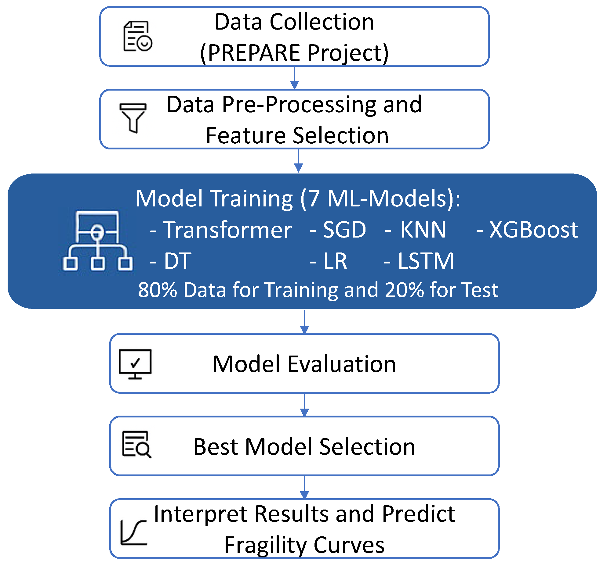
Figure 1. Overview of the workflow from data collection to fragility curve prediction.
Infrastructures 10 00279 g001
Figure 2. Correlation matrix of input features and output variables.
Infrastructures 10 00279 g002
Figure 3. SHAP Analysis: Feature importance and directional impact on building fragility models.
Infrastructures 10 00279 g003
Figure 4. Actual and predicted values by Transformer for PGA-SD.
Infrastructures 10 00279 g004
Figure 5. Actual and predicted values by Transformer for PGA-LD.
Infrastructures 10 00279 g005
Figure 6. Actual and predicted values by Transformer for PGA-84% NC.
Infrastructures 10 00279 g006
Figure 7. Actual and predicted values by Transformer for PGA-50% NC.
Infrastructures 10 00279 g007
Figure 8. Actual and predicted values by Transformer for PGA-16% NC.
Infrastructures 10 00279 g008
Figure 9. Actual and predicted values by Transformer for PGA-84% C.
Infrastructures 10 00279 g009
Figure 10. Actual and predicted values by Transformer for PGA-50% C.
Infrastructures 10 00279 g010
Figure 11. Actual and predicted values by Transformer for PGA-16% C.
Infrastructures 10 00279 g011
Figure 12. Training and validation loss curves of the Transformer model over 300 epochs using MSE loss.
Infrastructures 10 00279 g012
Figure 13. RMSE values for each ML model across different PGA levels (a) SD, (b) LD, (c) 84% NC, (d) 50% NC, (e) 16% NC, (f) 84% C, (g) 50% C, and (h) 16% C.
Infrastructures 10 00279 g013
Figure 14. Mean values of error metrics (a) MAPE, (b) MSE, and (c) RMSE for different ML models.
Infrastructures 10 00279 g014
Figure 15. Fragility curves generated by the Transformer model corresponding to different predicted PGA levels based on the full dataset.
Infrastructures 10 00279 g015
Figure 16. Fragility curves obtained using actual data set compared with predictions via Transformer based on all features and different PGA (a) SD, (b) LD, (c) 84% NC, (d) 50% NC, (e) 16% NC, (f) 84% C, (g) 50% C, and (h) 16% C.
Infrastructures 10 00279 g016
Table 1. Feature descriptions with units or types.
No.DescriptionUnit/Type
1Structural fundamental periods
2Right wall connection qualitygood/bad (categorical)
3Left wall connection qualitygood/bad (categorical)
4Total area of openings (windows/doors)m2
5Wall thicknessmm
6Wall lengthm
7Wall heightm
8Type of masonry usedfired/unfired (categorical)
9Height of bricksmm
10Length of bricksmm
11Brick staggering (overlap)mm
12Type of mortar usedconcrete/mud (categorical)
13Length of wall perpendicular to inspected wallm
14No. of internal walls perpendicular to inspected wallnumber
15No. of internal walls parallel to inspected wallnumber
16No. of internal walls perpendicular to back & parallel to inspected wallnumber
17Type of roofthatched/metallic (categorical)
18Orientation of roofparallel/orthogonal
19Presence of gableyes/no (binary)
20Height of gablem
21Spandrel heightm
Disclaimer/Publisher’s Note: The statements, opinions and data contained in all publications are solely those of the individual author(s) and contributor(s) and not of MDPI and/or the editor(s). MDPI and/or the editor(s) disclaim responsibility for any injury to people or property resulting from any ideas, methods, instructions or products referred to in the content.