Design of High-Precision Visual Localization System for Side-Seam Welding of Power Battery Modules

Abstract

Based on the problems of low efficiency, unstable accuracy, and weak anti-interference ability of manual localization for side-seam welding of square power battery module, this article designs a high-precision vision localization system for side seam based on machine vision. This system achieves automatic solving of welding reference points and start/end points through image preprocessing, an improved skeleton thinning algorithm, gray-scale projection feature separation, and a two-stage straight-line fitting algorithm design. The experimental results show that under the industrial site conditions covered in this experiment (normal lighting and conventional dust levels), the proposed method achieves an average localization error of 0.279 mm and a processing time of 384.3 ms per weld seam. It can meet the industrial requirements for automated welding of power battery modules and provides a referable technical solution for the engineering design of localization systems for side-weld welding of similar battery modules.

1. Introduction

Currently, the new energy vehicle industry is experiencing rapid development. The power battery serves as a core component of the entire vehicle, and its manufacturing quality directly impacts the vehicle’s endurance, safety, and service life. The square power battery modules have become the mainstream products in the market due to their high energy density, compact structure, and controllable cost [1]. The side-seam welding between the side plate and the end plate of the module is a key process. Localization deviation is prone to cause cold solder joint, solder skips, and weld deviation, directly affecting the structural strength and safety performance of the module.

The current artificial localization methods widely used in industrial sites suffer from low efficiency, significant accuracy fluctuations, and poor consistency, making it difficult to meet the demands of large-scale, high-quality automated production. The advantages of machine vision technology include non-contact, high precision, strong real-time performance, and wide adaptability. It has been widely applied in fields such as precision assembly, automatic welding, and online inspection [2]. However, the side seam of the power battery is slender and weak contrast. Traditional Hough transform, least squares method, and RANSAC (random sample consensus) algorithm find it difficult to simultaneously meet the requirements of accuracy, speed, and robustness. For this reason, from the perspective of engineering design and targeting the actual production requirements of automated welding for power battery modules, this paper designs a visual localization system for pre-weld side-seam localization. The system follows the technical pipeline of “image preprocessing → skeleton thinning and optimization → feature separation → two-stage straight-line fitting” to provide high-precision, stable, and real-time side-seam localization for welding equipment.

2. Literature Review

2.1. Research Status of Visual Localization

Visual localization technology involves analyzing and processing images captured by a camera, and using localization algorithms to calculate the positional coordinates of relevant areas [3]. Tanner et al. [4] analyzed the structural characteristics of the target’s shape and utilized morphological processing methods to extract the center point features to obtain position coordinate information. Li et al. [5] addressed the recognition and localization of stacked bagged goods on freight trains by using a monocular vision approach. They proposed a watershed transform for image recognition and employed image moments to achieve target localization. Tahir et al. [6] built a machine vision system to detect and locate the position of foreign bodies on high-speed paper. They primarily utilize traditional machine vision technology for feature extraction and employ clustering methods to quantify and locate foreign objects, effectively reducing detection and localization errors. Liu et al. [7] studied SURF (Speeded-Up Robust Feature) and RANSAC algorithms, organically integrated SURF and RANSAC technologies, and significantly improved the accuracy and reliability of matching by using the basic principle of SURF and the improved RANSAC algorithm. Wang et al. [8] proposed a method combining SURF and visual bag-of-words model with support vector machine to identify and locate workpieces, achieving the localization of multi-target workpieces. Xiao [9] proposed combining the Hough transform with the least squares method for line detection to obtain the localization information of points. Qi [10] invented a set of workpiece localization algorithms for dispensing machines using machine vision technology and proposed an improved SIFT (Scale Invariant Feature Transform) algorithm for workpiece matching of image blocks. Zhong et al. [11] used the minimum ellipse localization algorithm to achieve two-dimensional plane localization by modeling the cone sleeve of the air refueling system. He combined LHM (Lu, Hager, and Mjolsness) algorithm to achieve three-dimensional space localization and combined with the ROI (region of interest) region predicted by EKF (Extended Kalman Filter) to complete the stability of cone sleeve localization. Yin et al. [12] designed a visual localization method using a reflective tape scheme to meet the ARV (Autonomous and Remotely Operated Vehicle) requirements for close-range underwater docking. They proposed an improved Q-learning hybrid whale algorithm to optimize the Otsu (maximum inter-class variance method) function and combined it with the SRPnP (Simple, Robust and Fast Perspective-n-Point) algorithm to calculate the positions between the docking entities to achieve precise localization. Bi et al. [13] proposed a two-stage visual localization method for the localization error problem of micro-hole machining on vertical needle, utilizing sub-pixel and least squares methods to achieve precise localization of micro-hole locations. Existing research has primarily focused on optimizing individual algorithms, lacking a systematic approach to addressing issues such as the elongated side seams, weak texture, and strong interference characteristics of power batteries.

2.2. Research Status of Straight-Line Fitting

With the rapid development of machine vision technology, linear fitting and other related algorithms are constantly changing. Novikov [14] proposed a method for line detection and parameter estimation in contour images. This method primarily utilizes the property that a straight line is a special curve with zero curvature. In a sliding mode, a special mask is used to convolve the coordinate vectors of a finite length of pixels, thereby estimating the second derivative at each pixel location. When the second derivative is zero at all points, it indicates a straight line. Furthermore, this algorithm can also calculate the relevant parameters through the least squares method to obtain the end points of the line segment. Petkovic [15] proposed a least-squares straight-line fitting algorithm for computer and robot vision. The algorithm uses the coordinates of a point and its local gradient direction at the same time, and then fits an optimal straight line by minimizing the algebraic distance. This method can realize straight-line fitting through one data point, and for the same number of points, because it contains gradient information, the fitting accuracy is higher, and outliers can be excluded through gradient and distance. Fandejin et al. [16] proposed an improved least squares method. First, the image was processed to obtain the relevant feature point set, and then some parameters were introduced into the least squares method. The improved algorithm was repeatedly used for straight-line fitting to obtain the best weld line. The experimental results demonstrate that the improved least squares method can effectively and accurately fit a straight line, thereby achieving high-precision extraction of weld seam straight lines. Zhou et al. [17] put forward a method of multi-scale edge fitting to achieve high-precision and high-efficiency detection of ceramic filter screen, adding the idea of multi-scale to ensure the accurate extraction and screening of edges, focusing on a weighted least squares method, which introduces weight parameters in the calculation of the linear equation, to achieve accurate localization. The experimental results show that the algorithm has good real-time performance and high accuracy. Xiao [18] proposed a cascading deep-learning framework based on YoLov10 (You Only Look Once version 10) target detection and SoLov2 (Segmenting Objects by Locations version 2) instance segmentation. By segmenting the dual insertion holes of the pallet and extracting the corner points of the parallelograms, combined with the depth information from an RGB-D camera, visual localization of the pallet’s 3D center coordinates and orientation angle is achieved. Qin [19] proposed a visual SLAM (Simultaneous Localization and Mapping) method for indoor dynamic environment based on deep learning, which integrates YoLov8 (You Only Look Once version 8) target detection and LSD line feature extraction under the ORB_SLAM3 framework and combines epipolar geometric constraints to form a dual dynamic feature removal mechanism. It effectively solves the problem that the accuracy of pose estimation of mobile robot is reduced due to the interference of dynamic objects and significantly improves the localization robustness in complex scenes. Hough transform, least squares method, RANSAC, and deep-learning algorithm are common fitting algorithms, and their characteristics are shown in Table 1.

Table 1. Advantages and disadvantages of several commonly used straight-line fitting methods.

	Advantages	Disadvantages
Hough Transform	High robustness to noise	Low accuracy, high computational cost, relatively slow speed
Least squares method	Fast processing speed, high accuracy	Sensitive to noise, susceptible to outliers
RANSAC	High accuracy, good robustness	Relatively slow processing speed
Deep-learning algorithm	High accuracy, good robustness	Requires large training samples, high hardware requirements

As shown in Table 1, it is difficult for a single algorithm to balance efficiency, accuracy, speed, and robustness at the same time. Although the deep-learning algorithm has high accuracy and robustness, it needs a large number of training samples. The application scenario of this paper involves standardized modules, fixed workstations, and controlled lighting conditions, requiring the precise output of welding reference points, start points, end points, and weld seam direction within an extremely short time (<500 ms) for the robot to execute welding trajectory planning. This research focuses on the pre-weld localization stage, aiming to provide a high-speed and reliable front-end localization module for the above-mentioned complete vision system. Therefore, an improved straight-line fitting method based on the least squares method and the RANSAC algorithm can meet the engineering accuracy requirements, while offering engineering advantages such as low deployment cost and convenient debugging and maintenance. For the weld quality inspection part after the module weld seam is completed, since it is necessary to identify complex defect patterns such as porosity, cracks, undercuts, and lack of fusion on the weld surface, a deep learning-based image classification method is more suitable for weld quality inspection. This paper focuses on the design of a pre-weld seam localization system. The selected method can meet the requirements of high efficiency and precise localization. The weld quality inspection after module welding is not covered in this paper.

2.3. Insufficient Research

To sum up, the current research on localization technology using machine vision is mainly through image correlation processing, combined with line fitting and other algorithms to extract some feature information in the image, so as to realize the localization of objects in the image. The existing methods have the following shortcomings: first, the weld skeleton is easy to burr and break, and the localization stability is insufficient. Second, a single fitting algorithm is difficult to consider accuracy, speed and robustness. This paper effectively solves the above problems by constructing an integrated solution.

3. Research Methods

3.1. Design of the Image Preprocessing Module

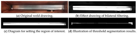
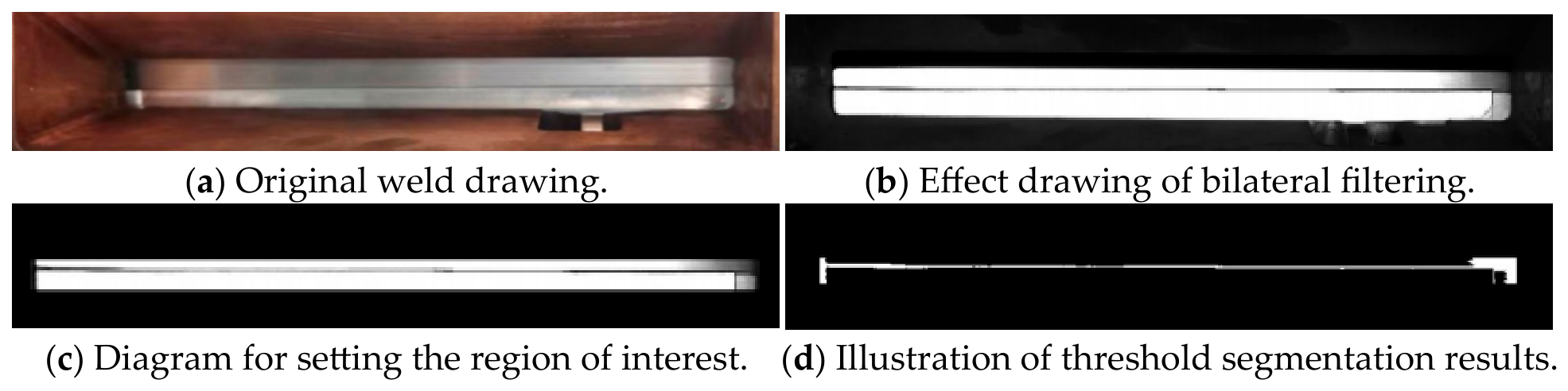
The side-seam pre-welding image collected by the vision system is shown in Figure 1a. Because the side-seam images collected at the industrial site are easily affected by complex factors such as uneven illumination, surface reflection, dust interference, edge shadow, and so on, direct feature extraction can easily introduce a lot of noise and reduce the localization accuracy and stability. Therefore, it is necessary to suppress interference and enhance effective features through the system preprocessing process to provide high-quality image basis for subsequent processing. Firstly, we need to perform grayscale processing on the image to reduce the interference of color information on subsequent analysis. Subsequently, bilateral filtering is used to suppress image noise while effectively preserving edge details and weakening the interference caused by uneven illumination and surface reflection. The results are shown in Figure 1b. Then, the region containing the side seam in the middle of the image is trimmed as the region of interest, and the irrelevant background is removed to reduce the subsequent calculation. The result is shown in Figure 1c. Finally, we employed the Otsu algorithm to perform threshold segmentation on the image of the area to be welded before side-seam welding, which was obtained after setting the region of interest. The purpose is to highlight the weld contour features, laying the foundation for subsequent skeleton extraction. The results are shown in Figure 1d.

Figure 1. Original drawing of front side-seam welding and effect drawing after image preprocessing.

3.2. Design of Localization Algorithm

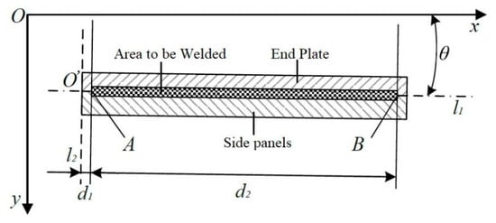
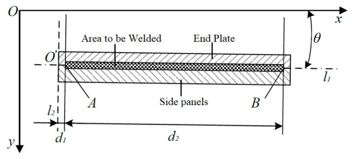
Through the preprocessing operation of the image before side-seam welding, the side-seam image of the module containing the area to be welded is obtained. The area to be welded before side-seam welding is approximately rectangular in shape. In order to correctly obtain the welding position, it is necessary to obtain the information such as the reference origin of side-seam welding, the starting point of welding, the weld length, and the inclination angle of the weld line. The principle is shown in Figure 2.

Figure 2. Schematic diagram of side-seam localization.

Point O is the origin of the image. According to the pre-weld image after pretreatment, first, it is necessary to fit an approximate horizontal line, L₁, that overlaps the area to be welded and an approximate vertical line, L₂, that aligns and overlaps the upper edge of the module end-plate side plate. The inclination angle of L₁ is θ (that is, the included angle between the welding direction and the x-axis). The point O′, where the two lines intersect, is the welding reference origin. D₁ is the offset distance determined along the welding direction according to the welding standard (that is, the distance o′a from the side plate end plate to the welding starting point), and D₂ is the welding length of the module to be completed (that is, the distance AB from the welding starting point to the welding end point). The weld width accuracy required by this design is ±0.5 mm. After calculation, the angle, θ, is generally between −0.22° and 0.22°.

In order to obtain the standard welding information, it is necessary to detect the coordinates of the reference origin, the linear equation of weld overlap, and the angle between the coordinate axis and the line. In this paper, a fast thinning algorithm is used to extract the skeleton centerline feature information of the binary region, and then the gray projection method is used to separate the obtained skeleton centerline from the point set of two straight lines’ fitting. Then, the straight-line fitting method is used to fit the approximate horizontal straight line in the welding direction and the vertical straight line overlapped on the upper surface of the end side seam. Finally, the intersection coordinates of the two straight lines are calculated as the reference point coordinates. The inclination angle of the straight line is calculated through the slope of the approximate horizontal straight line, and the coordinate information of the welding start point and the welding end point is obtained.

3.3. Feature Extraction

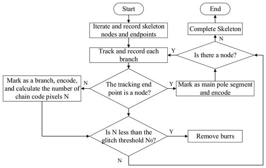
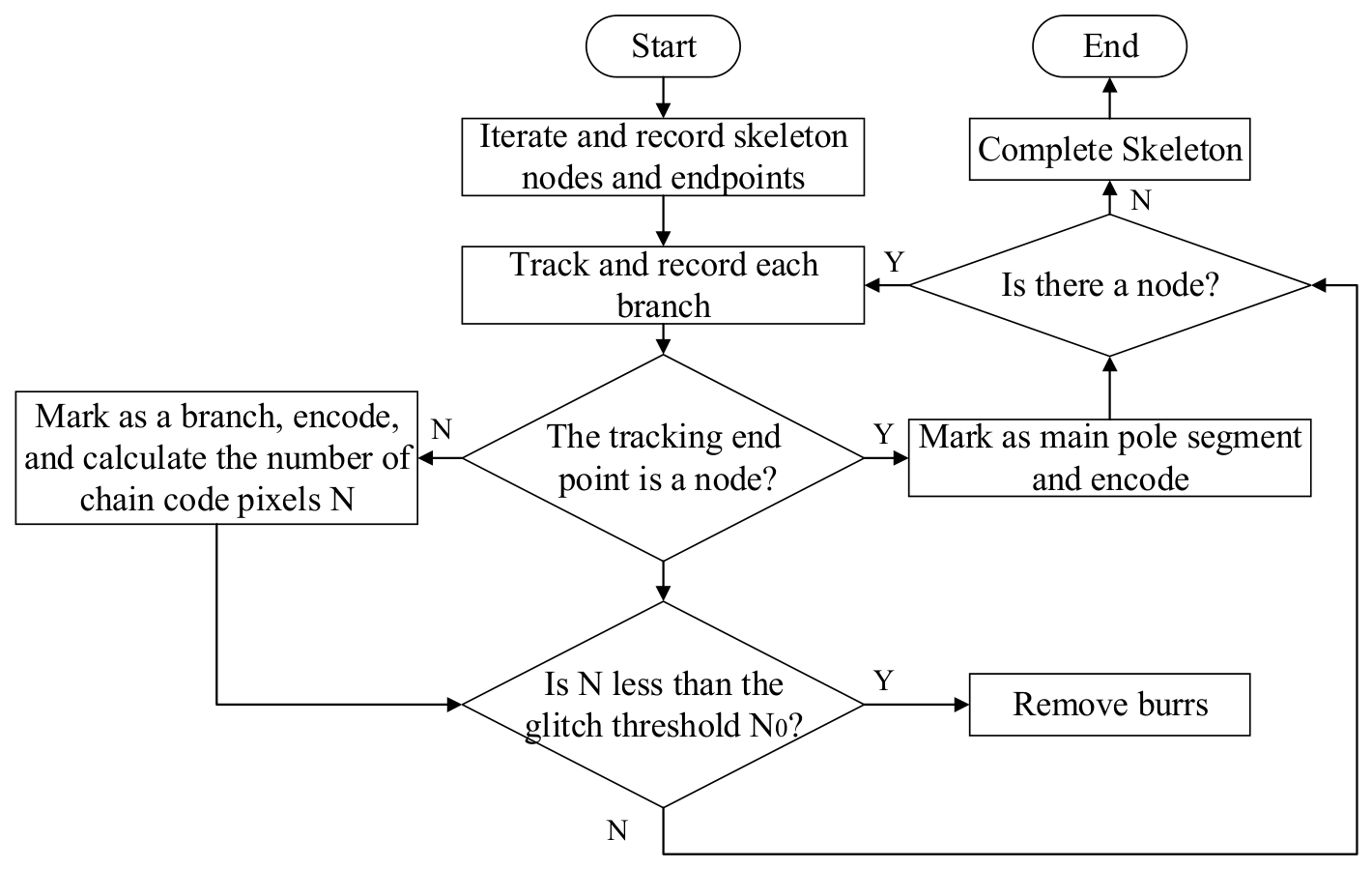
The extraction of the weld centerline is the core link of localization, which directly determines the quality of subsequent feature separation and line fitting. The traditional Zhang–Suen refinement method has high iteration efficiency and simple implementation. Still, it is easy to produce burr and disconnection problems at the weld edges and corners, affecting the continuity and smoothness of the skeleton, and thus reducing the localization stability [20]. Based on the traditional Zhang–Suen thinning algorithm, our research introduces an eight-connected chain code deburring optimization strategy to improve the quality of skeleton extraction. The specific measures are as follows:

(1)

According to the criteria of nodes and end points, all end points and nodes on the skeleton are determined iteratively, and their coordinates are recorded.

(2)

Each branch of the node is tracked by eight connected chain codes, and the branch coordinates are recorded. If the end point tracked by the branch is a node, this segment is marked as the trunk, and direction coding is performed from the end node to the start node. Otherwise, if the end point tracked by the branch is the end point, this segment will be marked as a branch. Perform directional encoding from the starting node towards the end point, and count the number of pixels, N, in the branch chain code.

(3)

Compare the number of branch chain code pixels, N, from the same node with the burr pixel threshold, N₀. If the number of branch pixels n is less than N₀, mark the branch as burr and delete the a burr. If each branch is greater than N₀, the next node is calculated.

(4)

When all nodes are traversed, the skeleton image is output.

The flowchart of the improved refinement extraction algorithm is shown in Figure 3.

Figure 3. Improved skeleton refinement flowchart.

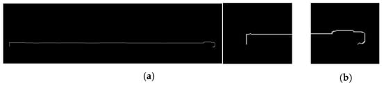
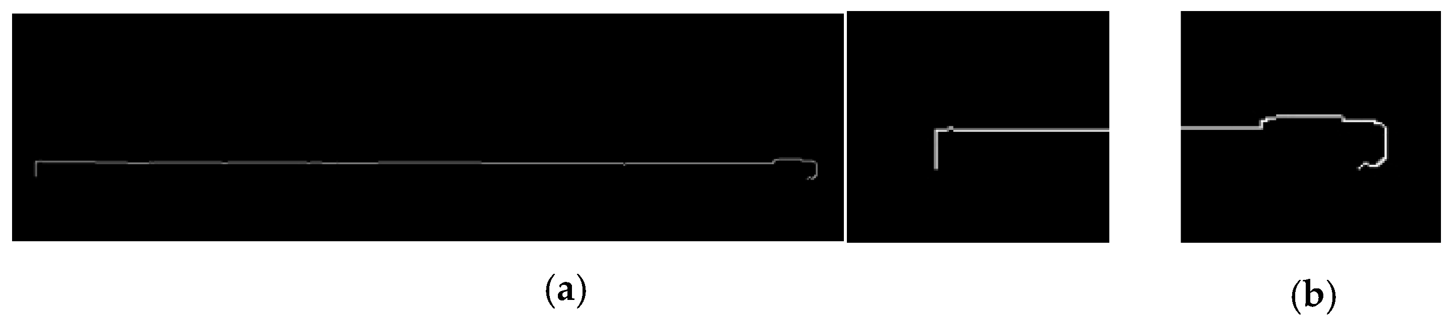
The skeleton of the area to be welded/extracted by the improved thinning algorithm is shown in Figure 4a, and the enlarged details are shown in Figure 4b. It can be seen from Figure 4 that the improved image is smoother, without burr and bifurcation, and can completely and correctly highlight the centerline features of the area to be welded.

Figure 4. Effect of improved skeleton extraction algorithm. (a) Original images after improvement of the skeleton algorithm. (b) Enlarged view of the details of the improved skeleton.

3.4. Set of Separation Points

Due to the influence of shadow, bright spot, and noise in the original image, after using parallel thinning to extract the skeleton centerline from the binary image after threshold segmentation, in addition to the target weld skeleton centerline, it also contains the projection contour lines above and below the end plate and many other useless contours. In order to obtain the reference origin information of the image before side-seam welding and realize localization, it is necessary to select the midpoint set of the target centerline and the projection contour lines on the upper surface of the end plate from all skeleton centerlines. In this paper, the pixel gray projection method is used to screen and separate the point set of the centerline of the weld skeleton and the projection contour line of the upper surface of the end plate.

The pixel gray projection method is a commonly used gray processing method in image processing that is used to analyze the pixel gray distribution of the image in a certain direction [21]. Let the image, f (x, y), represent the pixel gray value of the point (x, y), and the image region be [x₁, x₂] and [y₁, y₂]. The calculation expressions of vertical pixel gray projection and horizontal pixel gray projection for this region are shown in Equations (1) and (2):

$$G_v\left(x\right)={\int }_{y_1}^{y_2}f\left(x,y\right)dy$$

(1)

$$G_h\left(y\right)={\int }_{y_1}^{y_2}f\left(x,y\right)dx$$

(2)

In the formula, G_v(x) represents the vertical pixel grayscale projection, and G_h(y) represents the horizontal pixel grayscale projection.

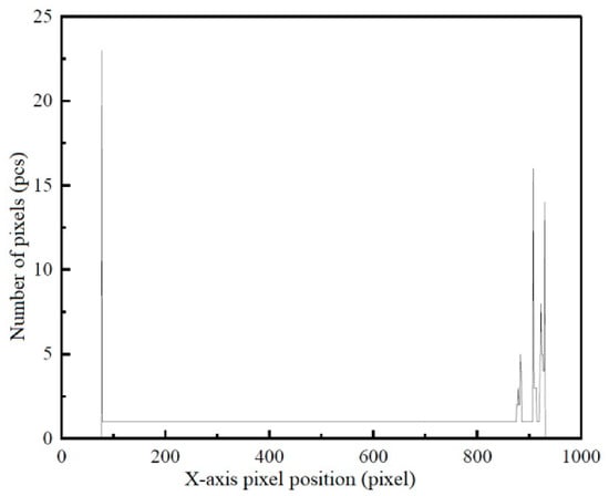
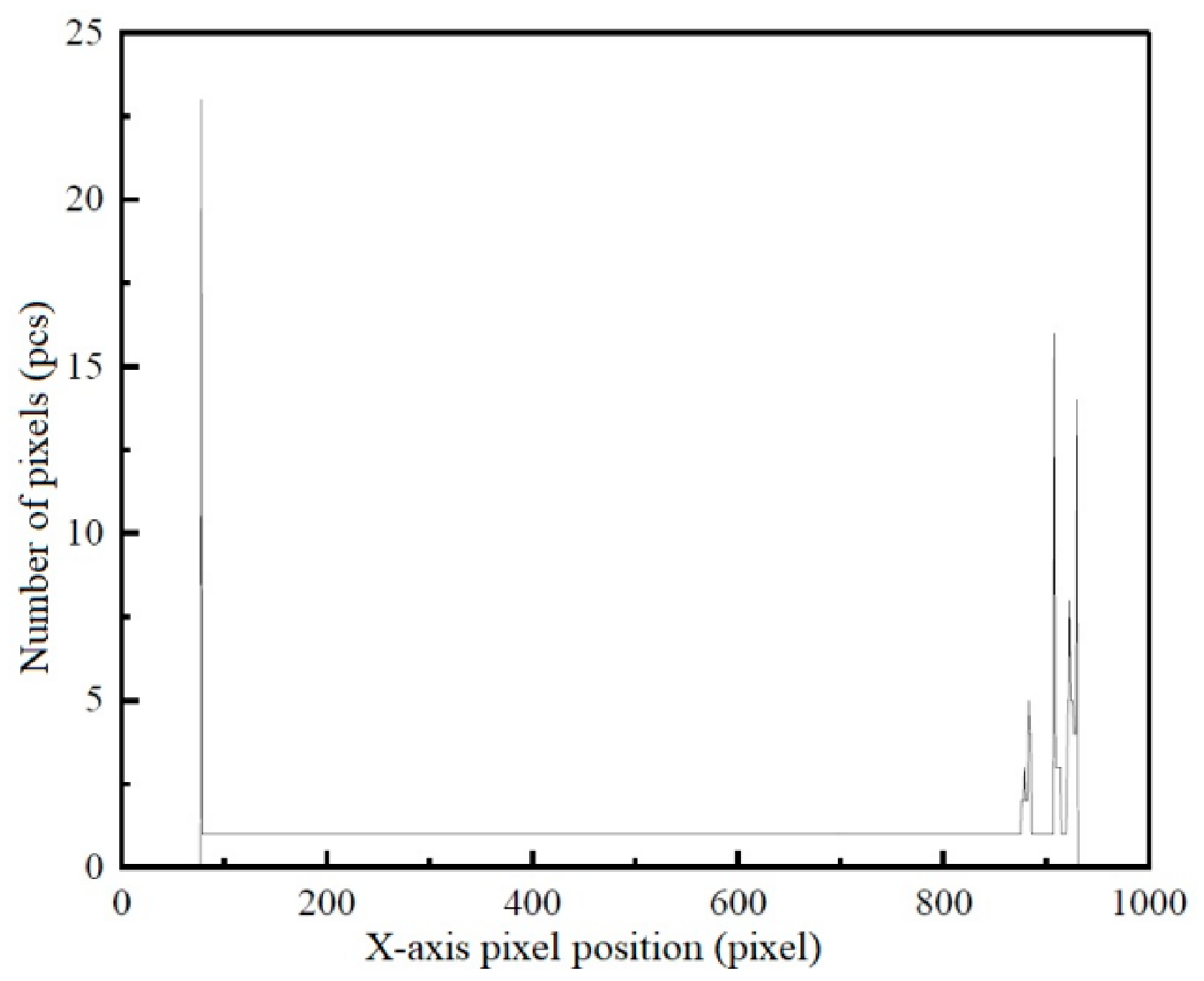
In the skeleton centerline image, the pixel distribution of the skeleton region containing some columns is significantly different from that in the background region. Based on this distribution feature, the number of white pixels in each column in the skeleton centerline image is counted to obtain the vertical gray projection of white pixels, as shown in Figure 5. Select the wave crest close to the image origin. The coordinates of the wave crest point are (78, 23), which correspond to the x-axis coordinate of the projected contour line on the upper surface of the end plate being 78. Select all white pixels in the skeleton centerline rendering corresponding to the three-pixel unit areas on the left and right of the x-axis coordinate as the point set M of the projection contour line on the upper surface of the fitting end plate.

Figure 5. Vertical grayscale projection diagram.

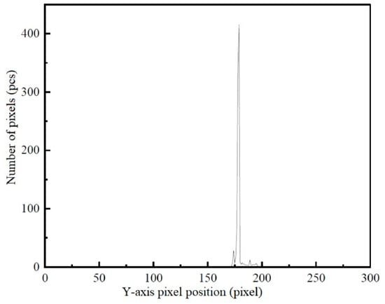
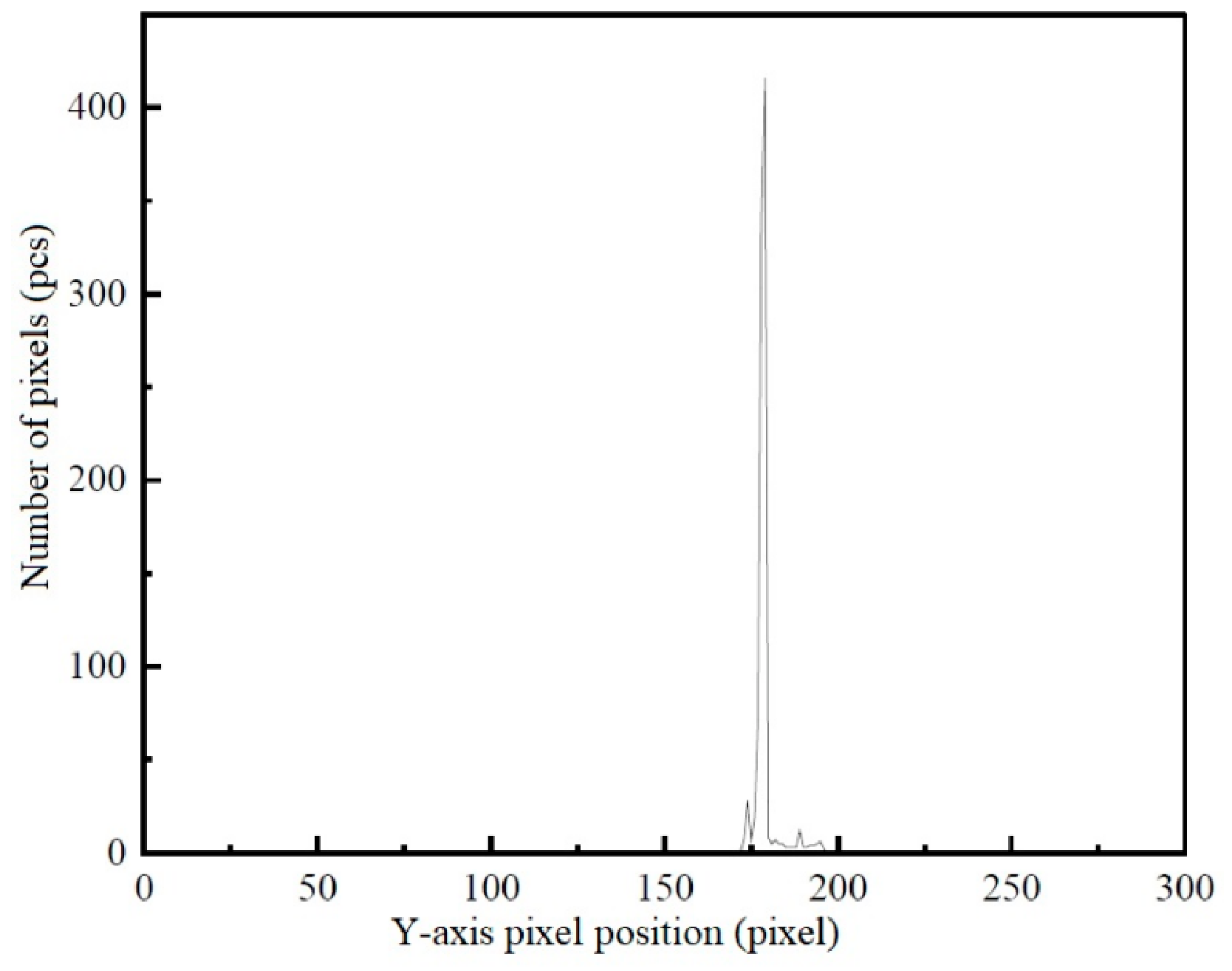
Similarly, the horizontal grayscale projection of white pixels can be obtained from the row pixel distribution characteristics of the skeleton area, as shown in Figure 6. Find the wave crest in Figure 6, corresponding to the coordinate point (179, 416) in the figure, which corresponds to the y-axis coordinate of the centerline of the weld skeleton, that is, 179. At the same time, in order to prevent the loss of effective point elements, all white pixel points in the skeleton centerline rendering corresponding to the five-pixel unit areas on the left and right of the y-axis coordinate are selected as the point set N for fitting the centerline of the weld skeleton.

Figure 6. Horizontal grayscale projection.

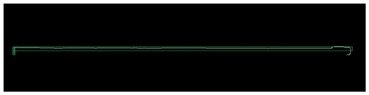
Except for the above two point sets, the points are irrelevant points, which will affect the accuracy of the side-seam position, so it is necessary to eliminate the irrelevant points. As shown in Figure 7, the area in the green box is the image to be retained, the area outside the green area of the image is the irrelevant point, the points in the horizontal green box are the point set M of the straight line fitting the welding direction, and the points in the vertical green box fit the point set N of the projected contour line on the upper surface of the end plate.

Figure 7. Separation of unrelated points.

3.5. Improved Straight-Line Fitting Algorithm

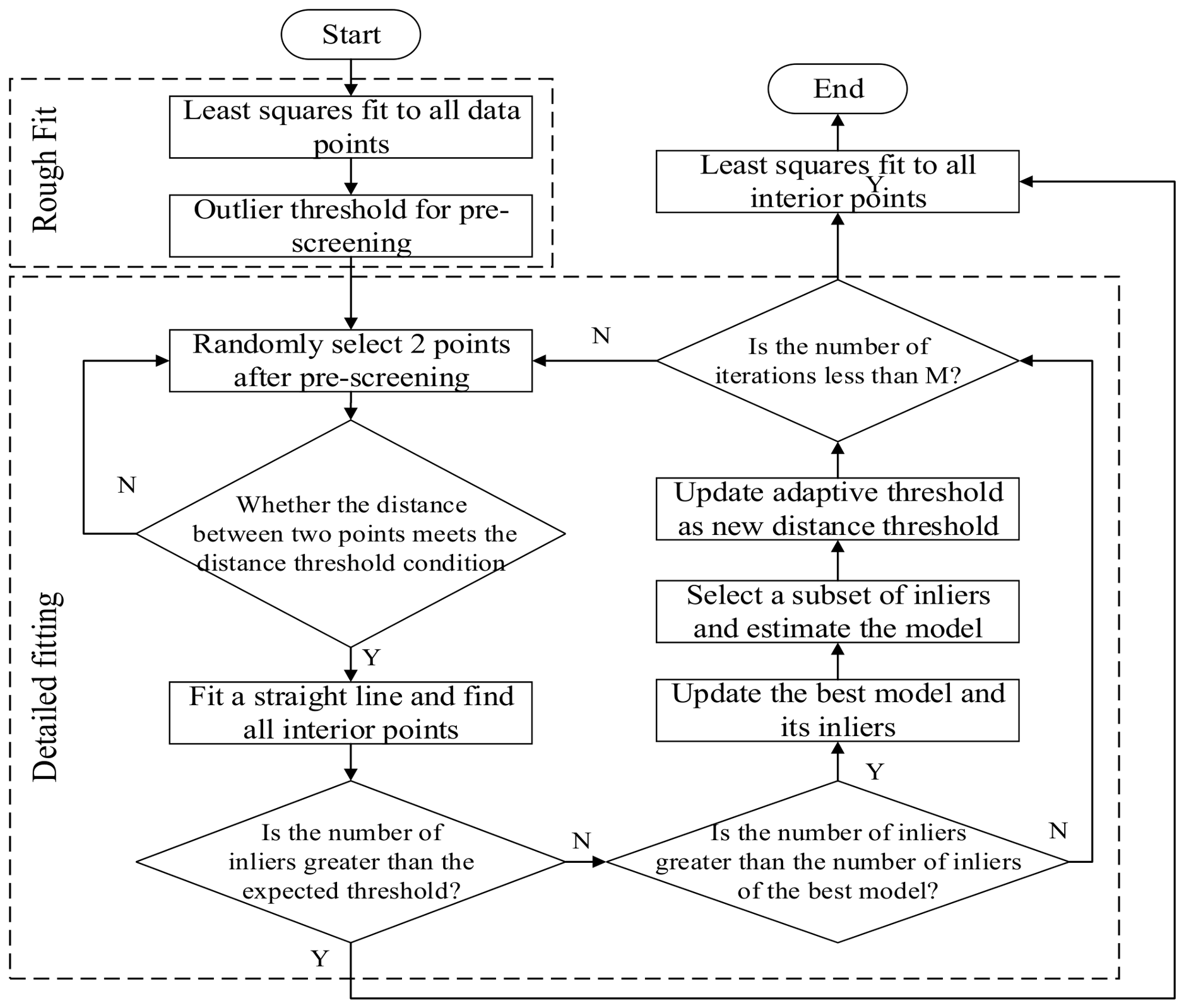
After the separation of point set M and point set N, in order to achieve accurate welding localization for the side seam of the module, the straight-line fitting method for the welding centerline is required. Commonly used line fitting algorithms include Hough transform, the least squares method, and RANSAC [22,23,24]. Among them, the least squares method has high processing speed and accuracy, but it is sensitive to noise and is easily affected by outliers. The RANSAC algorithm has high accuracy and good robustness, but its speed is relatively slow. The deep-learning algorithm has high accuracy and good robustness, but it requires a large number of training samples and has a relatively slow processing speed. Through the comprehensive comparative analysis of several line fitting methods, this paper designs an improved line fitting method based on the least squares method and the RANSAC algorithm. The flowchart of the improved straight-line fitting algorithm is shown in Figure 8.

Figure 8. Flowchart of the improved straight-line fitting algorithm.

The improved method is mainly divided into coarse and fine fitting stages, as follows:

(1)

The initial model data points are randomly selected, and noise outliers are selected with a certain probability. The greater the number of outliers, the greater the probability of selecting outliers, which will not only increase the amount of calculation and time consumed, but also reduce the efficiency.

To solve this problem, in the coarse fitting stage, the least squares method is used to perform the line coarse fitting for all data points, and the distance from each point to the coarse fitting line is calculated. Because the number of points in the skeleton centerline point set is far greater than the number of outliers, if the distance is greater than the initial set outlier threshold, the point is determined to be an outlier. The point can be deleted directly from the point set to avoid irrelevant calculation and random selection.

(2)

All the data points in the data point set cover a wide range. The initial model has no constraints when selecting data points, and the selected two points are not representative. If two points are too concentrated together and the distance between them is too small, it cannot be applied to all points, which can easily lead to a fitted linear model that differs significantly from the actual situation, and verification will also take longer.

To solve this problem, the first stage of fine fitting is carried out, and a distance threshold is set to restrict the distance between two randomly selected points by limiting the difference between the abscissa and ordinate coordinates to select representative points. The following formula shall be met:

$$\sqrt{{\left(x_a-x_b\right)}^2+{\left(y_a-y_b\right)}^2}\ge T_d$$

(3)

In the formula, (x_A, y_a) and (x_B, y_b) are points from the point set, and T_d represents the minimum distance threshold between two points.

(3)

After the best model is obtained by calculating and fitting with the initial model data points, it is necessary to re-select the data subset for straight-line fitting to replace the best model continuously. The selected data points are random, and repeated iterations can be close to the final result model. During this period, the number of iterations is long and time-consuming, and there are many unrelated calculations, reducing the fitting efficiency.

To solve this problem, the second stage of fine fitting is carried out. Because the initial model has some interior points, which meet the final result model, these interior points can be used as the data points of the next estimation model, and the adaptive threshold condition is used to speed up the iteration speed and reduce the number of iterations. The adaptive formula is as follows:

$$\left\{\begin{array}{c}{\mathrm{M}}_{\mathrm{m}\mathrm{i}\mathrm{n}}\le \mathrm{M}=\sqrt{{\mathrm{x}}_{\mathrm{i}}^2+{\mathrm{y}}_{\mathrm{i}}^2}\le {\mathrm{M}}_{\mathrm{m}\mathrm{a}\mathrm{x}}\\ {\mathrm{T}}_{\mathrm{a}}={\mathrm{M}}_{\mathrm{m}\mathrm{i}\mathrm{n}}/{\mathrm{M}}_{\mathrm{m}\mathrm{a}\mathrm{x}} \end{array}\right.$$

(4)

In the formula, M represents the distance from each point (x_i, y_j) in the point set to the origin, m_min and m_max are the minimum and maximum distances among all distances, and T_a represents the adaptive threshold coefficient.

3.6. Calculation of Welding Coordinates

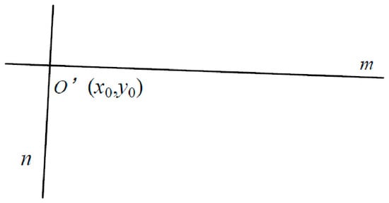
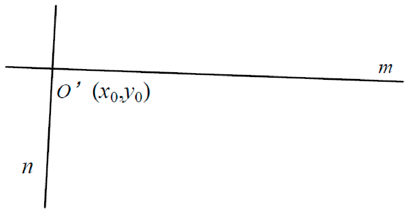
In order to determine the coordinate position of the starting and ending points of the weld, it is necessary to calculate the coordinate position of the intersection point of two fitted lines as the localization reference origin, and the low inclination line as the welding straight-line direction. The welding starting-point coordinates are calculated according to the offset distance determined from the reference origin along the welding direction according to the welding standard, and the end-point coordinates are calculated according to the welding length that the starting point needs to complete from the welding direction module. The line segment between the start and end of welding is the localization line segment before side-seam welding in this paper. The schematic diagram of the two straight lines’ fitting is shown in Figure 9.

Figure 9. Two straight lines’ fitting diagram.

Let the standard expressions of the straight lines, m and n, be as follows:

$$\left\{\begin{array}{c}{a}_{1}x+b_{1}y+c_1=0\\ a_{2}x+b_{2}y+c_2=0\end{array}\right.$$

(5)

where a₁, b₁, and c₁ are the parameters of fitted straight line m; and a₂, b₂, and c₂ are the parameters of fitted straight line n.

The intersection coordinates, O′(x₀, y₀), can be obtained from Equation (5):

$$\left\{\begin{array}{c}{x}_0={\displaystyle \frac{b_1{c}_2-b_2{c}_1}{a_1{b}_2-a_2{b}_1}} a_1{b}_2-a_2{b}_1\ne 0\\ y_0={\displaystyle \frac{a_2{c}_1-a_1{c}_2}{a_1{b}_2-a_2{b}_1}} a_1{b}_2-a_2{b}_1\ne 0\\ \mathrm{No} \mathrm{solution} \mathrm{or} \mathrm{infinite} \mathrm{solutions} a_1{b}_2-a_2{b}_1=0\end{array}\right.$$

(6)

The straight lines, m and n, fitted by the points in the two point sets in this article will not be parallel or coincide, so the coordinate of the reference point, O′, is $\left({\displaystyle \frac{{\mathrm{b}}_1{\mathrm{c}}_2-{\mathrm{b}}_2{\mathrm{c}}_1}{{\mathrm{a}}_1{\mathrm{b}}_2-{\mathrm{a}}_2{\mathrm{b}}_1}}, {\displaystyle \frac{{\mathrm{a}}_2{\mathrm{c}}_1-{\mathrm{a}}_1{\mathrm{c}}_2}{{\mathrm{a}}_1{\mathrm{b}}_2-{\mathrm{a}}_2{\mathrm{b}}_1}}\right)$.

The included angle, θ, between straight line m and the x-axis is as follows:

$${\mathsf{\theta }=\cos }^{-1}\left({\displaystyle \frac{b_1}{\sqrt{b_1^2+a_1^2}}}\right)$$

(7)

The formula for the straight-line distance between two points in the plane is as follows:

$$\mathrm{d}=\sqrt{{\left(x_a-x_b\right)}^2+{\left(y_a-y_b\right)}^2}$$

(8)

In the formula, (x_a, y_a) and (x_b, y_b) represent the coordinates of two points within the plane.

Based on this, it can be calculated that the coordinates of points A(x_a, y_a) and B(x_b, y_b), which are located at a specified distance along the designated angular direction of straight line m from the reference point, O′, are as follows:

$$\left\{\begin{array}{c}{x}_a={\displaystyle \frac{b_1{c}_2-b_2{c}_1}{a_1{b}_2-a_2{b}_1}}+{\displaystyle \frac{b_1{d}_1}{\sqrt{b_1^2+a_1^2}}}\\ y_a={\displaystyle \frac{a_2{c}_1-a_1{c}_2}{a_1{b}_2-a_2{b}_1}}+{\displaystyle \frac{a_1{d}_1}{\sqrt{b_1^2+a_1^2}}}\end{array}\right.$$

(9)

$$\left\{\begin{array}{c}{x}_b={\displaystyle \frac{b_1{c}_2-b_2{c}_1}{a_1{b}_2-a_2{b}_1}}+{\displaystyle \frac{b_1\left(d_1+d_2\right)}{\sqrt{b_1^2+a_1^2}}}\\ y_b={\displaystyle \frac{a_2{c}_1-a_1{c}_2}{a_1{b}_2-a_2{b}_1}}+{\displaystyle \frac{a_1\left(d_1+d_2\right)}{\sqrt{b_1^2+a_1^2}}}\end{array}\right.$$

(10)

where d₁ and d₂ are the offset distance and welding length from the reference point to the starting point of welding, that is, the length of line O′A and AB.

To ensure the reproducibility of the straight-line fitting method proposed in this paper and to clarify the influence of parameters on performance, the core parameter configurations of this design method are as follows:

(1)

The maximum number of RANSAC iterations is set to 200 (experimental verification shows that the model has converged after 20 iterations; 200 is set as the upper limit to ensure sufficient convergence). The inlier distance threshold is set to 3 pixels (approximately 0.08 mm), and the stopping criterion is either an inlier ratio ≥ 95% or reaching the maximum number of iterations.

(2)

The least squares method has no additional hyperparameters. The outlier rejection threshold adopts the statistical 3σ criterion, where points with residuals greater than three times the root mean square error are determined as outliers.

(3)

T_d constrains the minimum distance between two randomly sampled points to avoid model degradation caused by selecting two points that are too close to each other. If T_d is too small (<30 pixels), the model becomes susceptible to local noise; if it is too large (>80 pixels), it may fail to sample enough candidate points in short-weld-seam scenarios. In this paper, T_d is set to 50 pixels, which is approximately 38% of the weld seam width (3.5 mm ≈ 130 pixels), balancing model stability and sample sufficiency.

(4)

Tₐ is used to filter the spatial distribution range of the inlier set during the iteration process. A larger Tₐ value results in a more concentrated spatial distribution of retained inliers, leading to faster model convergence but at the cost of potentially losing edge information. A smaller Tₐ value yields a more dispersed inlier distribution, enhancing model generalizability while increasing the number of iterations. In this paper, Tₐ is set to 0.5, which serves as a trade-off value balancing convergence speed and model accuracy.

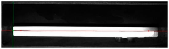
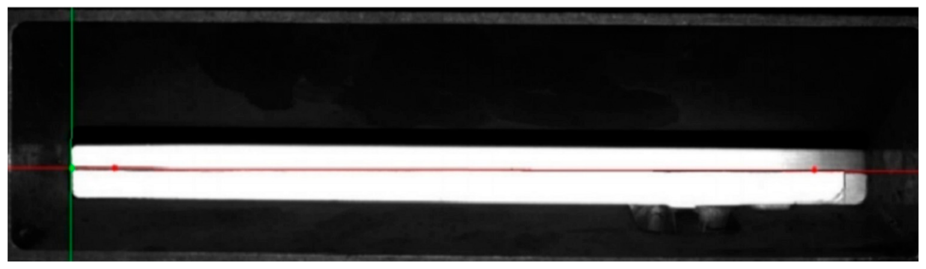
The effect drawing of localization before side-seam welding is shown in Figure 10. The coordinates of the reference point, O′ (green point in the figure), are obtained through the intersection of two red lines. The coordinates of the starting point, A (the red point on the left in the figure), are obtained from the offset distance, and the coordinates of the ending point, B (the red point on the right in the figure), are obtained from the welding length.

Figure 10. Side-seam pre-weld localization effect.

4. Results and Analysis

The experimental object of this paper is a new energy enterprise mass-produced square power battery module. The overall size of the module is 420 mm long, 180 mm wide, and 120 mm high; the side-seam length is about 130 mm, and the width is about 3.5 mm. The industrial site has strict requirements on the welding localization accuracy: the localization error should be controlled within ±0.5 mm, the processing time of a single weld should not exceed 500 ms, and the repeated localization accuracy should not exceed 0.5 mm.

The experimental hardware uses an industrial visual acquisition and processing platform, including a CCD industrial camera (DMK, The Imaging Source, Bremen, Germany) with a resolution of 2592 × 1944 and a frame rate of 15 fps, a fixed focus lens with a focal length of 16 mm, a brightness adjustable annular shadowless LED light source, an i7-12700h processor, an RTX 306 graphics card, an industrial computer with 16 GB memory, and a communication module supporting OPC UA (OPC Unified Architecture) protocol. It can communicate with the PLC and the plant MES (Manufacturing Execution System) system in real time to ensure data interaction and production coordination.

The software platform is based on the Windows 10 64-bit operating system and utilizes the Visual Studio 2022 development environment. It combines the OpenCV (version 4.5.1.) image processing library with the C++ programming language to facilitate algorithm development, debugging, and deployment, ensuring both algorithm efficiency and industrial compatibility.

4.1. Experiment on an Improved Linear Fitting Algorithm

After separating the point sets, the Hough transform, the least squares method, the RANSAC, and the algorithm used in this paper are used to fit the two filtered point sets, M and N, in the skeleton centerline image as straight lines, m and n; and the angles, θ and ϕ, with the X axis and Y axis and the fitting times, t₁ and t₂, of the two straight lines are analyzed, respectively. The parameters of each method in the comparative experiment are set as follows: Hough transform is implemented by OpenCV standard, and the accumulator threshold is set to 100 after experimental optimization. The least squares method is realized by standard without additional parameters. The maximum number of iterations of RANSAC is set to 1000, and the inner point distance threshold is set to 3 pixels. The results are shown in Table 2.

Table 2. Comprehensive comparison of localization accuracy and repeatability of different algorithms.

	Template Image	Hough Transform	Least Squares Method	Random Sampling Consensus Algorithm	Algorithm of This Article
$\mathsf{\theta }\left(°\right)$	0	0.35	0.26	0.22	0.14
$\mathrm{\phi }\left(°\right)$	0	0.47	0.31	0.27	0.17
$t_1\left(\mathrm{m}\mathrm{s}\right)$		27.8	2.9	5.3	3.9
$t_2\left(\mathrm{m}\mathrm{s}\right)$		20.6	2.2	4.1	3.3
MAE (mm)		0.74	0.54	0.49	0.279
RMSE (mm)		0.96	0.69	0.54	0.336
Repeatability (mm)		≤0.06	≤0.02	0.1~0.15	≤0.05

It can be seen from the above table that when fitting straight lines by Hough transform, it is easy to fit multiple straight lines together, which will interfere with the final result and cause large errors. The detection time of the Hough transform is approximately ten times that of the least squares method; its practical application is inefficient and lacks real-time performance. The least squares method achieves the fastest speed and the best repeatability among the several methods, but there are some outliers in the point set, leading to a large deviation in the results. The fitting accuracy of the RANSAC algorithm is high, and the fitting process needs to eliminate outliers iteratively, which is time-consuming. The improved algorithm can eliminate the interference of outliers and achieve high accuracy. Although the computation time and repeatability accuracy are slightly increased compared to the least squares fitting, the time is reduced by approximately one-quarter compared to the RANSAC algorithm, and real-time performance can still be guaranteed.

4.2. Localization Experiment Prior to Side-Seam Welding

The localization experiment before side-seam welding of the battery module mainly verifies whether the localization accuracy can reach the required accuracy and whether the localization time can reach the required time. Five square-shaped power battery modules were selected for the side-seam localization welding experiment after assembly, and a total of 20 side seams need to be welded. Record the position of the welding end point of each side-seam localization and compare it with the coordinate value measured manually, that is, the error between the ideal welding end point and the actual welding end point. The experimental results of side-seam localization are shown in Table 3.

Table 3. Experimental results of side-seam localization.

Side-Seam Number	Ideal Welding End-Point Coordinates /mm	Actual Welding End-Point Coordinates /mm	Error Value /mm	Algorithm Detection Time /ms
1	(158.43, 64.41)	(158.17, 64.68)	−0.243	379
2	(158.04, 64.16)	(158.19, 64.36)	0.247	385
3	(157.92, 64.09)	(157.79, 64.21)	−0.176	408
4	(157.99, 64.14)	(157.72, 64.38)	−0.359	362
5	(158.28, 64.33)	(158.57, 64.54)	0.356	387
6	(157.96, 64.11)	(157.61, 64.32)	−0.408	403
7	(158.35, 64.32)	(158.59, 64.16)	0.291	382
8	(158.21, 64.25)	(157.95, 64.34)	−0.283	396
9	(158.07, 64.25)	(158.31, 64.53)	0.366	384
10	(158.21, 64.21)	(158.09, 64.39)	0.217	391
11	(158.15, 64.04)	(158.02, 63.68)	−0.383	377
12	(157.98, 64.01)	(158.23, 63.85)	0.295	401
13	(158.29, 64.18)	(158.43, 64.27)	0.165	364
14	(157.91, 64.21)	(157.75, 64.53)	−0.357	386
15	(158.13, 64.08)	(158.37, 64.21)	0.273	372
16	(157.96, 64.31)	(158.13, 64.12)	0.255	387
17	(158.05, 64.04)	(158.31, 64.23)	0.322	385
18	(158.31, 64.14)	(158.06, 63.95)	−0.314	392
19	(158.37, 64.09)	(158.59, 64.25)	0.272	371
20	(158.16, 64.35)	(157.95, 64.11)	−0.319	374

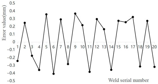
Draw a line chart according to the error value between the 20 ideal positions and the actual localization positions, as shown in Figure 11.

Figure 11. Weld localization Error Line Chart.

It can be seen from Table 3 and Figure 11 that the absolute average error between the welding end-point coordinates and the ideal end-point coordinates detected by the method used in this paper is 0.279 mm, which does not exceed the maximum error limit of ±0.5 mm. The average detection time is 384.3 ms, with high accuracy and good real-time performance, which can meet the actual production requirements of side-seam welding of the power battery module.

4.3. Side-Plate Welding Experiment of Battery Module

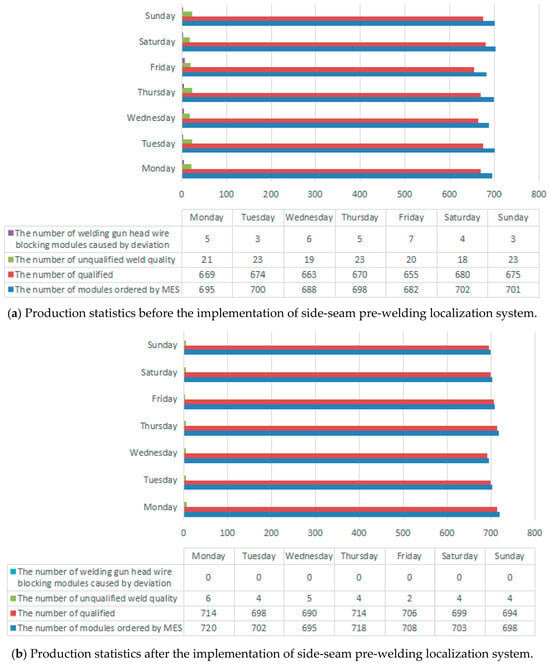
In order to verify the stability of the localization system before side-seam welding, the design uses the 9-core module of the ternary aluminum shell lithium battery as the experimental object to verify the localization system before side-seam welding. The validation cycle is one week, daily double shift. The work content is to record the number of single-mode modules sent by MES system, the number of qualified modules, the number of unqualified modules, and the number of repair welding modules and disassembly modules caused by weld problems.

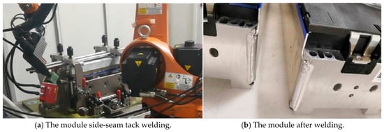
After the battery modules are stacked, the modules enter the fixed platform of the welding room together with the stacking trolley. After the trolley is in place, the trolley localization cylinder automatically extends to position the trolley on the welding workbench. The welding robot starts to move from the origin to a safe position outside the reserved weld. Position the four reserved welds of the module in turn before side-seam welding and complete the four-side-seam welding after localization. The automatic localization welding process of the side seam of the module and the photos of the module after welding are shown in Figure 12.

Figure 12. The module side-plate welding and weld quality after welding.

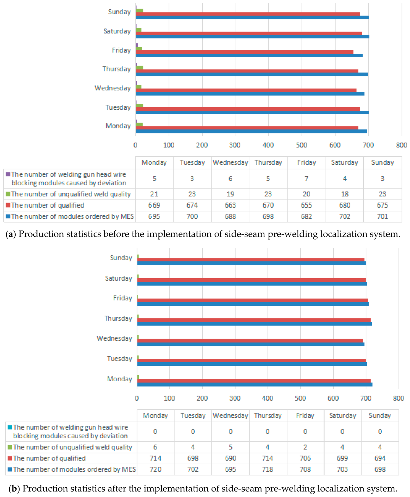
Figure 13 is a histogram of production related data measured during the test. This bar chart records the number of single mold groups sent to the production line, the number of qualified welding modules, the number of modules requiring repair welding of welds, and the number of modules due to unqualified welds every day in the week of the test. According to the test statistics, the welding quality of the side seam of the module was significantly improved by using the pre-welding localization system of the side seam of the module, and the one-time welding qualification rate of the side seam can reach more than 99%. Due to the weld deviation, the number of welding gun line blockage was reduced to zero, which minimizes the module disassembly caused by unqualified welding and reduces the production cost.

Figure 13. Module production status information.

5. Discussion

Through systematic algorithm optimization, this paper effectively improves the localization accuracy and real time. The improved skeleton thinning algorithm eliminates the burr disconnection, ensures the continuity and smoothness of the skeleton, and lays the foundation for high-precision localization. The two-stage linear fitting combines the speed advantage of the least squares method and the robustness advantage of the RANSAC algorithm, effectively restraining the influence of outliers and adapting to complex industrial conditions.

In this paper, for extreme lighting conditions, bilateral filtering is used to suppress uneven lighting in the preprocessing stage, and Otsu adaptive threshold segmentation is robust to image contrast and brightness changes. The following strategies are proposed to further enhance the adaptability to extreme environments: (1) Adaptive exposure control is introduced to dynamically adjust the camera exposure time according to the image gray distribution. (2) A multi-angle annular light source lighting scheme was adopted to reduce single-direction reflective interference. (3) The image-enhancement algorithm based on Retinex theory is explored to improve the identifiability of weld features under low-illumination conditions.

The localization accuracy of this method is mainly affected by the reflectivity of the material surface in the image preprocessing stage. The difference of light reflection characteristics of different materials (aluminum alloy, stainless steel, nickel-plated steel, etc.) will lead to the contrast change between the weld area and the background. The bilateral filtering used in this paper can suppress the interference of high reflection while preserving the edge details. Otsu adaptive threshold segmentation does not depend on the fixed gray threshold, and has a certain adaptability to the changes in image gray distribution caused by different reflectivity. For the materials with extreme reflectivity (such as mirror polished aluminum), it is recommended to use with annular shadowless light source and polarizer to reduce mirror reflection interference.

6. Conclusions

This article designs a high-precision visual localization method that improves the skeleton thinning algorithm and linear fitting algorithm to address the issues of low efficiency and poor accuracy in manual localization for side-seam welding of power battery modules. We have achieved stable and high-precision side-seam localization by suppressing complex interference through image preprocessing, refining the skeleton to generate a smooth centerline, accurately separating feature lines through grayscale projection, and solving for welding coordinates through two-stage linear fitting.

The experimental results show that the average localization error of this method is 0.279 mm, and the average time of a single weld is 384.3 ms. It runs stably under the industrial conditions of this experiment, and preliminarily verifies its engineering feasibility. The research results can provide technical support for the intelligent manufacturing of power battery modules.

References

- Zuo, P.W.; Zhu, P.P.; Shao, L.Q. Development characteristics and trend analysis of new energy vehicle power battery industry. Automot. Abstr. 2021, 1, 1–7. [Google Scholar] [CrossRef]
- Truong, V.D.; Wang, Y.F.; Won, C.; Yoon, J.A. Deep Learning-Based Machine Vision System for Online Monitoring and Quality Evaluation During Multi-Layer Multi-Pass Welding. Sensors 2025, 25, 4997. [Google Scholar] [CrossRef] [Scilit] [PubMed]
- Li, W.J. Research on Key Technologies of Vision Localization System for Lead Welding Machine. Master’s Thesis, Harbin Institute of technology, Harbin, China, 2021. [Google Scholar] [CrossRef]
- Tanner, E.; Granade, S.; Whitehead, C.A. Autonomous rendezvous and docking sensor suite. Proc. SPIE Int. Soc. Opt. Eng. 2003, 5086, 329–339. [Google Scholar] [CrossRef] [Scilit]
- Li, H.; Yang, Y.; Zeng, R.; Zeng, F. Research on the recognition and location method of stacked bagged agricultural materials based on monocular vision. Image Signal Process. 2021, 11, 229–233. [Google Scholar] [CrossRef] [Scilit]
- Tahir, M.N.; Khalid, Z.; Aslam, A. Online, Real-Time and Robust Detection and Localization of Foreign Objects on Paper Surface Using Machine Vision and Clustering. Mach. Vis. Pract. 2022, 3, 1–6. [Google Scholar] [CrossRef] [Scilit]
- Liu, J.L.; Bu, F.L. Improved RANSAC features image-matching method based on SURF. J. Eng. 2019, 19, 123–129. [Google Scholar] [CrossRef] [Scilit]
- Wang, Z.; Ma, X.; Mu, C.; An, H. Research on Adhesive Workpiece Recognition and Localization Based on Machine Vision. Int. Conf. 2019, 6, 213–219. [Google Scholar] [CrossRef] [Scilit]
- Xiao, M. Research on Wafer Localization System Based on Machine Vision. Master’s Thesis, Shanghai Jiaotong University, Shanghai, China, 2013. Available online: https://kns.cnki.net/kcms2/article/abstract?v=7jvqSXIa2LXqrKSOhQVhAGCnoi00ifyx23neaKs7yp_6kjdSvsF2EIixp_EUTTkBLpXyTRGEGGLey3ahFLy0uAuiz_KJVbrs9Di7nODHGQj3vfSmPI7onV-IZtz4cCR5ojOMKOYt29VzFhBR469w24h_i1H5sQdwRSaTE2JiIAE=&uniplatform=NZKPT (accessed on 1 June 2026).
- Qi, Z.L. Research on Workpiece Localization of Dispensing Machine Based on Machine Vision. Master’s Thesis, Nanchang University, Nanchang, China, 2018. Available online: https://kns.cnki.net/kcms2/article/abstract?v=7jvqSXIa2LXyi_T74ZoGdwsh6bWs5r7IRnTz-xiM0eNi4BiMpENNaVIP_-noRxnaD7uJjbsh4Z9wghBgwzx6LDFExCkOdO47-iRaufOJu2zLriqse-qXQz7D5bZtxzOvjNA46fVaNwk5uSoob4lh_QbYkXMt2A9tgq2rHfjSF7I=&uniplatform=NZKPT (accessed on 1 June 2026).
- Zhong, Z.W.; Qin, Y.; Wang, H.L.; Su, Z.K.; Yao, P.; Li, N. Vision based tracking and localization of autonomous aerial refueling cone. Electron. Opt. Control 2019, 26, 71–77. [Google Scholar]
- Yin, G.C.; Wu, C. An ARV docking visual localization algorithm based on reflective tape scheme. Robot 2022, 44, 574–588. [Google Scholar] [CrossRef]
- Bi, Y.F.; Jiang, G.D.; Mei, X.S.; Huang, W.W.; Wang, G.C. Research on visual localization technology for chip packaging vertical needle micro hole processing. J. Xi’an Jiaotong Univ. 2021, 55, 59–67. [Google Scholar]
- Novikov, A.I.; Melnikova, E.S.; Ustyukov, D.I. Straight Line Detection Method for Images Based on the Properties of Curvature. Int. Conf. Digit. Signal Process. Appl. 2020, 6, 121–129. [Google Scholar] [CrossRef] [Scilit]
- Petkovic, T.; Loncaric, S. Using Gradient Orientation to Improve Least Squares Line Fitting. Comput. Robot Vis. 2014, 8, 235–243. [Google Scholar] [CrossRef] [Scilit]
- Fan, D.J.; Yang, L.X.; Ding, L.; Liang, D. Research on weld line extraction based on improved least square method. Hot Work. Process 2018, 47, 217–220+224. [Google Scholar] [CrossRef]
- Zhou, J.; Dong, Z.H.; Ren, J.Y.; Zheng, F.; Li, J.P. Ceramic filter quality detection method based on multi-scale edge fitting. Acta Photonica Sin. 2021, 50, 173–184. [Google Scholar]
- Xiao, Z.M.; Wang, Z.G.; Qian, D.H. Visual detection and localization of pallet insertion holes based on deep learning. Autom. Instrum. 2026, 2, 6–9+14. [Google Scholar] [CrossRef]
- Qin, J.R.; Wang, Y.G.; Cong, X.L.; Zhou, L.Y. A visual localization SLAM method for mobile robots in indoor dynamic environments based on deep learning. J. Detect. Control 2025, 47, 71–79. [Google Scholar] [CrossRef]
- Hu, X.; Ouyang, H.; Hou, Z.C.; Li, H.P. Pointer skeleton extraction based on improved ZS thinning algorithm. Autom. Instrum. 2021, 36, 51–56. [Google Scholar] [CrossRef]
- Han, S.; Lee, T.B.; Heo, Y.S. Semantic-Aware Face Deblurring with Pixel-Wise Projection Discriminator. IEEE Access 2023, 11, 11587–11600. [Google Scholar] [CrossRef] [Scilit]
- Wei, S.Q. Intelligent Detection of Hot Spot of Photovoltaic Module Based on Infrared Image. Master’s Thesis, Zhejiang University, Hangzhou, China, 2020. [Google Scholar] [CrossRef]
- Lei, X.Q.; Zhang, Y.D.; Ma, W.S.; Hu, L.Q.; Zuo, X.L. Least square fitting and error evaluation of bearing roller crown profile. Opt. Precis. Eng. 2018, 26, 2039–2047. [Google Scholar] [CrossRef] [Scilit]
- Ma, S.; Guo, P.; You, H.; He, P.; Li, H. An Image Matching Optimization Algorithm Based on Pixel Shift Clustering RANSAC. Inf. Sci. 2021, 21, 145–149. [Google Scholar] [CrossRef] [Scilit]
Disclaimer/Publisher’s Note: The statements, opinions and data contained in all publications are solely those of the individual author(s) and contributor(s) and not of MDPI and/or the editor(s). MDPI and/or the editor(s) disclaim responsibility for any injury to people or property resulting from any ideas, methods, instructions or products referred to in the content. |
© 2026 by the authors. Licensee MDPI, Basel, Switzerland. This article is an open access article distributed under the terms and conditions of the Creative Commons Attribution (CC BY) license.