


Abstract
The Berry phase plays a central role in modern electronics and acts as a foundation for a wide range of phenomena, from the anomalous Hall effect to topological insulators and valleytronics. However, in conventional analytical treatments, its geometric origin frequently stays abstract and unreachable. A thorough paradigm for computational visualization that clarifies the emergence and implications of the Berry phase in quantum electronic systems is presented in this paper. The simulation begins with a spin-½ model in a rotating magnetic field and uses real-time spin precession and field rotation tracking to demonstrate geometric phase accumulation on the Bloch sphere. Key ideas for comprehending tunable topological devices are revealed by the dynamic redistribution of Berry curvature and associated Berry-flux evolution when the framework is further extended to time-dependent Hamiltonians that reflect oscillating fields or shifting mass terms. Users can see local spin textures and phase progression within the Brillouin zone by mapping each k-point in momentum-space modules to a small Bloch sphere. Topology is linked to quantifiable device phenomena by a hybrid real- and momentum-space animation that links geometric phase evolution with observable transport behavior such as quantized Hall responses and Landau orbits. Together, these interconnected modules provide an interactive framework for exploring Berry-phase-related geometric and transport phenomena across complementary quantum-mechanical representations. Finally, these visualizations form an interactive and pedagogically rich toolset that unites geometric quantum theory with practical implications for next-generation electronic and spintronic devices.
1. Introduction
1.1. Berry Phase in Quantum Mechanics
In quantum mechanics, when a system undergoes a slow, cyclic change in its parameters and returns to its initial configuration, the wavefunction can acquire an additional phase beyond the usual dynamical phase associated with energy and time evolution. This extra, path-dependent phase is known as the “Berry Phase”. The Berry phase has become an increasingly valuable concept in the design and characterization of electronic and quantum devices. In topological materials [1,2], for example, the Berry curvature acts as an effective magnetic field in momentum space, thereby enabling novel transport phenomena such as the anomalous Hall effect and topological charge pumping [3], phenomena that can be directly harnessed in device architectures for low-power electronics and spintronics [4]. Topological charge pumping is the quantized transport of charge that occurs when a system undergoes a cyclic and adiabatic variation of its parameters, where the net charge transferred per cycle is determined solely by the geometric properties of the path in parameter space, such as the integrated Berry curvature or associated Chern numbers, rather than by the specific dynamics of the system. In graphene-based resonators, researchers have demonstrated that a small change in magnetic field can toggle a π Berry phase on and off, causing abrupt energy shifts in angular-momentum states, an effect with clear implications for highly sensitive optoelectronic devices [5]. A direct experimental manifestation of the Berry phase has been observed in graphene-based resonators, where a small change in magnetic field can toggle a π Berry phase on and off, producing abrupt shifts in the angular-momentum energy states [5]. This provides a measurable physical signature of the Berry phase and demonstrates how the geometric phase can directly influence the electronic energy spectrum. This sharp, controllable change could be used to make very sensitive electronic or optical devices. Moreover, in layered two-dimensional systems, the ability to tune Berry curvature and related orbital magnetic moment via external fields opens pathways to device control of valleytronics and quantum transport [6]. These utilities collectively emphasize that, in addition to fundamental physics, Berry-phase engineering offers a robust toolkit for device-level innovation in electronics, photonics, and quantum information technologies.
For an analogy point of view, it can be understood as a “memory” of the path taken in parameter space, rather than depending completely on the initial and final states. The Berry phase [7] represents a geometric contribution to the total quantum phase acquired by a state undergoing slow cyclic evolution. It is essential to emphasize that the Berry phase is different from the dynamical phase since it only depends on the shape of the path traced in parameter space [4]. This can be intuitively understood by comparing it to parallel transport of a vector on a curved surface where the vector retains a memory of the path and rotates upon returning to its starting position even in the absence of twisting. Similarly, the solid angle traced on the Bloch sphere is proportional to the Berry phase in quantum systems like a spin-1/2 in a rotating magnetic field (slow or adiabatically rotating field) [8]. It should be emphasized that the Berry phase is not restricted to electrons or to spin − systems. The spin − case considered here represents the simplest two-level quantum system and provides a convenient framework for visualizing geometric-phase accumulation on the Bloch sphere. More generally, geometric phases can arise whenever a quantum state evolves cyclically through parameter space under appropriate conditions, including systems with higher spin, quasiparticle states, and other multilevel quantum systems. Thus, is a model choice for the present simulation rather than a fundamental requirement for the existence of a Berry phase. This idea is fundamental to contemporary condensed matter physics and supports spintronics, topological insulators, and the quantum Hall effect, among other phenomena.
The scientific novelty of the present work lies primarily in the integration and interactive visualization of several geometric and topological phenomena within a common computational framework. Rather than treating Berry phase, Berry curvature, topological indices, semiclassical dynamics, and magnetic-field-driven quantum behavior as isolated calculations, the developed simulator allows physical parameters to be varied dynamically while their corresponding geometric and physical responses are visualized in real time. The framework combines Bloch-sphere evolution and Berry-phase accumulation with momentum-space Berry-curvature mapping, mass-dependent Dirac-band behavior, semiclassical trajectories, and Landau quantization. This integrated approach enables direct exploration of how changes in model parameters influence geometric phase, local Berry-curvature distributions, and associated dynamical responses. Thus, the contribution of the present work is not a new definition of Berry-phase quantities, but an interactive computational framework that connects their analytical foundations with dynamic visualization and quantitative verification.
Within this integrated framework, the individual simulations represent distinct physical models rather than components of a single unified Hamiltonian. The spin-dynamics module illustrates geometric-phase accumulation during magnetic-field evolution, while the Dirac-band model is used to examine Berry curvature and mass-dependent topological behavior. Semiclassical transport is treated separately to demonstrate the influence of Berry curvature on particle trajectories, whereas the Landau-quantization module describes magnetic-field-dependent energy levels and cyclotron behavior. Although these models share the common theme of Berry-phase-related physics, each module employs its own governing equations, assumptions, and parameter set appropriate to the phenomenon being illustrated.
Understanding of Berry Phase Through Analogies
As discussed in the previous section, the concept of the Berry phase can be intuitively understood through simple geometric analogies. Let us consider a compass that always points north while traveling a closed loop around a hill. Upon returning to the original starting location, the compass needle may appear slightly rotated compared to its initial orientation. The precise route traveled around the hill creates an extra rotation even though the actual position stays unaltered. This additional rotation acts as a counterpart to the Berry phase, which is an effect that is entirely dependent on the path’s shape rather than traversal speed or duration.
This can also be understood by considering another comparison. The example of a ribbon looped around a finger without any initial twist leads to a similar interpretation. Even though the ends of the ribbon have not been changed, a twist may form when the finger is moved along a closed path in space and returned to its original location. This twist is an accumulation of a geometric phase due to the trajectory’s topology and curvature. This geometric memory is essentially embodied by the Berry phase, which is dependent on the path’s shape in parameter space rather than the system’s time history. The quantum wavefunction gains an extra phase even if the physical configuration reverts to its initial state. This concept is a key focal point in understanding various mechanisms in topological materials, the quantum Hall effect, and a variety of molecular and condensed matter systems, demonstrating the fundamental connection between quantum physics and geometry.
1.2. Mathematical Understanding of Berry Phase
In quantum mechanics, the state of a system is described by a wavefunction , whose time evolution is governed by the time-dependent non-relativistic Schrödinger equation. The corresponding energy-dependent evolution gives rise to the usual dynamical phase, expressed as follows:
where is the instantaneous energy of state and ℏ is the reduced Planck constant.
However, in the case of slow and cyclic change, we will notice a different observation. If the system changes slowly (adiabatic) and eventually returns to its initial parameters, something interesting happens. The wavefunction comes back to the same physical state, but may gain an extra phase called the Berry phase:
- → usual dynamical phase.
- → geometric phase depending only on the path taken.
Berry Phase Formula
For a parameter-dependent Hamiltonian with eigenstate :
- = closed path in parameter space.
- is called the Berry connection [9].
- The integral gives the total geometric phase accumulated over the cycle.
So, in plain language: if we multiply our wavefunction by a small twist at each step along the path, then sum all twists over the loop. That is the Berry phase.
2. Materials and Methods
2.1. Computational Framework and Numerical Implementation
All simulations were implemented in Python 3.11 using the numerical parameters specified for the respective physical models. The computational framework was developed to provide interactive simulation and visualization of Berry-phase phenomena, including Bloch-sphere dynamics, geometric-phase accumulation, momentum-space Berry curvature, and related quantum-transport behavior.
Time-dependent evolution was evaluated using a fourth-order Runge–Kutta (RK4) scheme, while momentum-space quantities were calculated over a discretized momentum-space grid. The numerical resolution, integration time step, number of sampling points, and parameter ranges were selected to provide stable numerical results while maintaining interactive computational performance. Numerical convergence was assessed by refining the temporal and momentum-space discretization and confirming that the principal calculated quantities and observed trends remained unchanged within the adopted numerical resolution.
The simulation environment was developed using Python with NumPy for numerical calculations, Matplotlib (version 3.10) with the TkAgg backend for two- and three-dimensional visualization, and Tkinter and ttk widgets for the graphical user interface. The software architecture allows interactive modification of simulation parameters and visualization of the corresponding response. Separate computational processes were used for animation and data recording to maintain responsiveness during interactive operation. The program also provides CSV export functionality for subsequent quantitative analysis.
The computational framework was developed primarily for conceptual visualization and investigation of Berry-phase phenomena. Accordingly, some simulation modules employ generic parameters, normalized or arbitrary units, and simplified physical assumptions to facilitate interactive visualization and computational efficiency. The simulations are therefore not intended as quantitative predictions for specific materials, devices, or experimental systems unless the corresponding material-specific parameters and physical models are independently incorporated and validated. The calculated results should consequently be interpreted within the assumptions and limitations of the respective models. The simulation code is provided for research and educational use, with appropriate citation and acknowledgment.
2.2. Berry-Phase Model and Geometric Representation
To provide an intuitive representation of the Berry phase, the quantum state was visualized as evolving along a closed trajectory on the Bloch sphere. When the system completes a cyclic evolution and returns to its initial physical configuration, the quantum state can acquire an additional geometric phase determined by the path followed in parameter space.
A spin-½ system subjected to a slowly rotating magnetic field was used as the representative two-level model. The direction of the magnetic field follows a closed conical trajectory on the Bloch sphere, and the resulting geometric phase is related to the solid angle enclosed by this trajectory. The Berry phase is expressed as follows:
where Ω represents the solid angle subtended by the closed trajectory on the Bloch sphere. Within the adiabatic formulation, the resulting geometric phase depends on the geometry of the path rather than the rate at which the closed trajectory is traversed.
2.3. Interactive Bloch-Sphere Simulation and Visualization
An interactive Bloch-sphere simulation module was developed to visualize the evolution of the quantum state and the associated geometric phase. In the simulation, the magnetic-field vector is rotated around the z-axis at a constant polar angle, producing a conical trajectory on the Bloch sphere. User-controlled parameters allow the magnetic-field orientation, angular velocity, and cone angle to be varied interactively, enabling direct visualization of their influence on spin evolution and geometric-phase accumulation.
The solid angle subtended by the closed trajectory determines the corresponding Berry phase and is calculated according to
The primary goal of this simulation code is to illustrate conceptual features of Bloch-sphere dynamics, Berry phase, and related topological phenomena. For accessibility and visual clarity, the program uses a number of generic parameters, arbitrary units, and simplified assumptions. It is not guaranteed to be flawless for quantitative prediction, device design, or engineering validation, and it might not accurately reflect experimental findings. The authors and contributors make no assurances or warranties regarding accuracy, completeness, or suitability for any specific purpose, even though every attempt has been made to ensure that the underlying ideas are valid. The user uses this code at their own risk and judgment. As long as proper citation and acknowledgment are provided, redistribution or modification is allowed under the original open-use intent.
3. Results
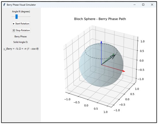
The developed Tkinter-based interactive framework enables real-time visualization of both the solid angle, Ω, and the corresponding Berry phase, γBerry, as shown in Figure 1. Variation of the polar angle through the interactive slider produces an immediate change in the accumulated Berry phase, demonstrating its dependence on the geometry of the closed trajectory on the Bloch sphere. The results therefore provide a direct visual representation of the relationship between the enclosed solid angle and geometric-phase accumulation. Other controls like start and stop allow users to experience visualization of the cyclic evolution of the field vector, making the geometric nature of the phase accumulation visually unique. Before going much deeper into its importance in condensed matter, spin systems, and topological physics, researchers can use this tool to gain an intuitive knowledge of how the Berry phase develops from adiabatic cyclic evolution in parameter space.
Figure 1.
First-generation Berry phase visual simulator.
3.1. Additional Visualization and Quantitative Verification of the Berry Phase
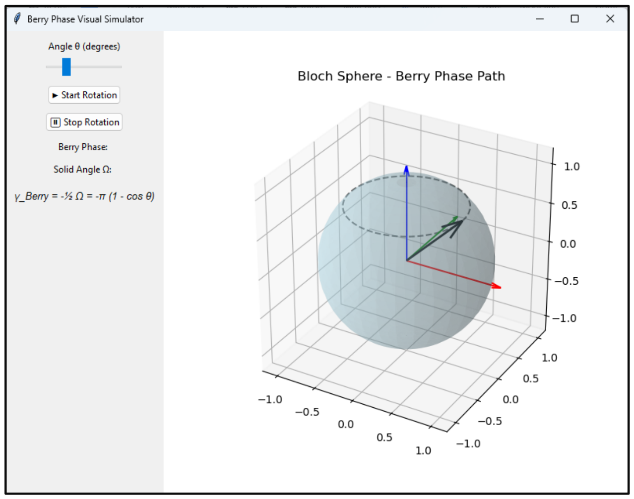
As discussed earlier, a user can experience an intuitive and dynamic visualization of the emergence of the Berry phase for a spin-½ particle under the condition of a slowly rotating magnetic field. The Bloch sphere is a signature of the state space of the spin system, where a black arrow extending from the origin represents the time-dependent magnetic field vector B(t). The instantaneous direction of B was defined as , where φ is the azimuthal angle changing continuously with time. This vector spins around the vertical z-axis while maintaining its magnitude constant, creating a constant polar angle θ with respect to it. From a physics point of view, this is equivalent to a homogeneous magnetic field whose strength stays constant, but its direction changes adiabatically. The arrow’s tip encloses a solid angle Ω by tracing a conical surface on the Bloch sphere as the magnetic field rotates.
The purple arrow shown in the figure represents the spin vector S(t) of the particle. For the adiabatic limit, the spin moreover aligns with the instantaneous magnetic field direction; however, due to the geometric nature of its evolution, the spin gets an additional phase shift that is not related to dynamical energy changes. This additional phase represents the geometric phase accumulated during the cyclic evolution. After a full 360° rotation of the magnetic field, the spin returns to its original orientation in physical space but accumulates a Berry phase.
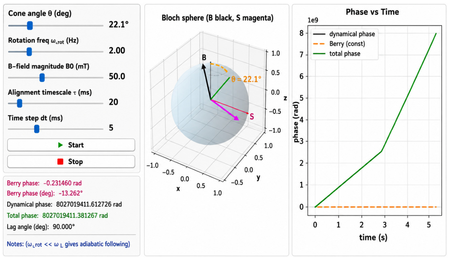
The trajectory of B(t) on the Bloch sphere is shown in the visualization as a dashed circular path at the tip of the magnetic field arrow. Since the solid angle Ω determines the phase using the preceding equation, the enclosed area on this surface directly represents the geometric origin of the Berry phase, as follows: Equation (5) During the simulation, both the instantaneous Berry phase (in degrees and radians) and the field rotation angle ϕ are displayed numerically in real time (see Figure 2). As the magnetic field rotates, the Berry phase increases proportionally to the fraction of the completed cycle, with its sign reversing if the rotation direction is inverted. As we adjust the θ-slider, it modifies the cone angle dynamically and enables users to observe that larger cone angles result in correspondingly larger Berry phases. When θ = 0°, the magnetic field path shrinks to a point (Ω = 0), and no geometric phase is accumulated.
Figure 2.
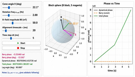
Second-Generation Berry Phase Simulator: Showing various sliders where various other parameters can be changed and associated Berry and dynamical phase can be viewed in a panel. Purple arrow is instantaneous spin vector. Black arrow is magnetic field direction.
The analytical formulation also provides useful benchmark limits beyond the representative θ = 45° case. From γB = −π(1 – cos θ), the Berry phase is exactly zero at θ = 0°, increases to ∣γB∣ = π/2 at θ = 60°, and reaches ∣γB∣ = π at θ = 90° for a complete rotation. These limiting and intermediate cases provide additional reference points for evaluating the simulator response and confirm the expected monotonic dependence of the geometric phase on the solid angle enclosed by the rotating field. In addition, reversing the direction of the closed trajectory reverses the sign of the Berry phase while preserving its magnitude, consistent with the orientation dependence of the geometric phase.
To verify the simulation quantitatively for one case, the following representative parameters were used: total field rotation ϕ = 55.98°, solid angle Ω = 1.84 rad2, and full-cycle Berry-phase magnitude || = 0.92015 rad. The theoretical relation predicts = −0.92 rad, which agrees precisely (|Δ| < 1.5 × 10⁻⁴) with the computed value. Alternatively, substituting Ω = 2π(1 − cos θ) yields cos θ ≈ 0.707, corresponding to θ ≈ 45°, consistent with the canonical textbook case. The simulation also captures the fractional accumulation of Berry phase during incomplete rotations. For the field rotation angle ϕ = 55.98° (fraction f = ϕ/360 = 0.1555), the instantaneous phase build-up is
matching the visualized geometric twist observed in the interface. The Berry phase evolves linearly with the fraction of the completed rotation, as stated in the code, according to the agreement between the simulated and analytical values:
In the discussed case, is the total Berry phase gathered over one full cycle, and represents the instantaneous angular parameter of evolution in the parameter space. The modulo operation ensures that the accumulated phase is confined within the range. By convention, the simulation shows the magnitude of the Berry phase for visual clarity, whereas the orientation of the geometric progression is encoded by the physical sign. The strong agreement between the analytical predictions and simulation results confirms the accuracy and reliability of the model, offering a physically consistent and numerically precise representation of Berry-phase accumulation in spin systems. Numerical convergence was also examined for the time-driven oscillating-mass simulations by varying both the fourth-order Runge–Kutta (RK4) integration time step and the k-space grid density. Successive reductions in the RK4 time step produced negligible changes in the calculated trajectories and accumulated geometric response, while increasing the k-space grid resolution resulted in convergence of the computed Berry-curvature distribution and local Chern estimates. In particular, the locations and relative magnitudes of the Berry-curvature features and the associated temporal evolution of the Chern estimate remained unchanged upon further refinement. These tests indicate that the reported dynamic behavior is numerically stable and is not an artifact of the selected temporal or momentum-space discretization.
Table 1 shows the symbols, their meaning, and displayed units used in our simulators.
Table 1.
List of various symbols, their meaning, and associated units.
3.2. Computational Framework for Band Dirac Hamiltonian
For a two-band Dirac model [10] with
Here (a vector function of momentum k) represents the effective field in the pseudospin (Bloch) space that appears in the two-level Hamiltonian.
A simple Hamiltonian often used to illustrate Berry curvature is
where is a “mass term” (gap).
kx and ky are coupling along the x and y directions, respectively.
The Berry curvature for the lower-energy band is
and the normalized Berry-flux contribution is [11] shown below:
For this simple model,
- for .
- for .
Steps toward finding the correct k-space patch that maps to the Bloch-sphere cap
The boundary between included and excluded directions on the Bloch sphere is given by
Relation between solid angle, Berry phase, and k-space integral
For a spherical cap of polar (cone) angle , the solid angle is The Berry phase for a spin-½ (lower band) corresponding to that cap is
If the Bloch-sphere cap of polar angle corresponds to the disk in k-space of radius:
then the integral of curvature over that disk (in polar coordinates) is
We can compute that integral analytically:
Let , . Then,
- In the limit the integral approaches , so the total (infinite-plane) integrated curvature is . Dividing by gives the familiar half-integer Berry-flux contribution for a single continuum Dirac cone for the lower band (for and the chosen sign conventions).
- If , we can replace as appropriate; the expression above with makes the absolute-value dependence explicit.
Using gives . Hence,
So, the integral over the correct k-space disk equals the Berry phase exactly.
Therefore, the expected numeric identities are
and the corresponding partial Berry-flux contribution is
Here, in the preceding discussion, is the Dirac mass parameter (or gap parameter) appearing in the effective two-band Hamiltonian and should not be interpreted as the ordinary inertial mass of a particle. Therefore, does not imply an imaginary or physically negative particle mass. Rather, the sign of determines the orientation of the mass term and reverses the sign of the associated Berry curvature and Berry-flux contribution. At , the mass term vanishes and the energy gap closes at the Dirac point (), where the two bands become degenerate. Consequently, the Berry curvature of an individual isolated band is not well defined exactly at this degeneracy. Changing the sign of therefore describes a mass-sign reversal through the gap-closing condition rather than a change to an imaginary particle mass.
3.3. Addition of Momentum Space Tab
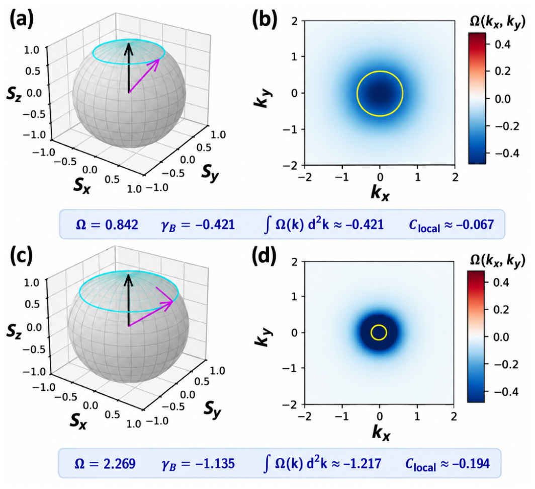
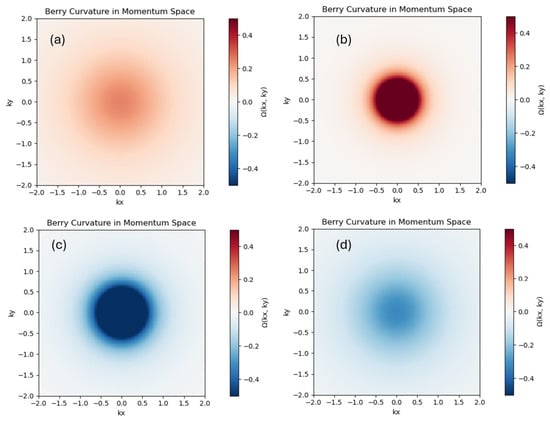
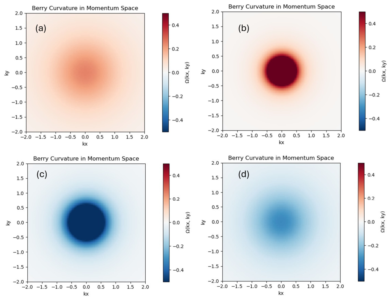
To complement the real-space Berry-phase visualization on the Bloch sphere, a parallel momentum-space representation was implemented to illustrate the emergence of Berry curvature and its connection to topological invariants. The model employs a two-band massive Dirac Hamiltonian, where the mass term acts as a tunable control parameter for band inversion. The calculated Berry curvature is plotted over a discretized Brillouin zone, while the numerical integration of yields the partial Berry-flux estimate . As gets closer to zero, the Berry curvature becomes very localized near the Dirac point, creating a clear yellow hot spot on the momentum-space map (see Figure 3). This behavior shows how unique the gauge connection is when the energy gap closes, which is the start of a topological transition. On the other hand, when is very positive or negative, the curvature spreads out smoothly and the Chern number gets closer to zero, which means that the regime is topologically trivial (see Figure 4). Figure 4 shows that when the base mass is low, the Berry curvature is mostly positive near the Dirac point, which means that the local band geometry adds a positive Berry flux [12]. When the base mass goes up, the sign of changes, which means that there is an inversion of band character between the conduction and valence bands. This change is a topological phase crossover, where the curvature “flips” its direction in momentum space. The sign change in as mass increases is a sign of band inversion-driven topology, which is what the analytical prediction says.
Figure 3.
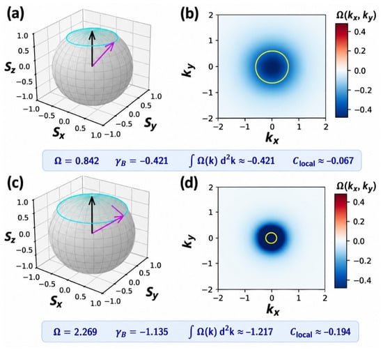
Geometric connection between the Berry phase on the Bloch sphere and Berry curvature in momentum space. (a–d) The Bloch-sphere representation shows spin vectors tracing circular cones with polar angles and , corresponding to two distinct solid angles and . S solid angles (a,b) and for large solid angles (c,d) are plotted. The larger cone (smaller ) subtends a smaller solid angle, resulting in a weaker geometric phase, while the smaller cone (larger ) encloses a greater portion of the sphere, leading to an enhanced Berry phase . In the corresponding momentum-space maps, the Berry curvature forms localized peaks near the Dirac point. The yellow circular contour indicates the region in -space integrated to obtain the local Chern estimate .
Figure 4.
(a–d) Snapshots of Berry curvature evolution in momentum space as a function of base mass . For small m, the Berry curvature is positive (a,b) and localized near k = 0. As m increases, the curvature changes sign, becoming negative (c,d) and redistributing in the kx-ky plane.
This interactive visualization therefore connects the geometric concept of the Berry phase with the momentum-space distribution and integrated flux of Berry curvature. We have examined the simulator by choosing different values (slider movement) and found various outputs of Chern number displayed in the panel (see Table 2). In the two-band Dirac model, the mass term determines both the sign and localization of the Berry curvature near the Dirac point. When , the curvature is negative around , producing a negative contribution to the Chern number. Conversely, when , the curvature reverses sign, indicating a topological inversion of the band structure. In this low-energy continuum model, the integrated Chern number approaches , rather than an integer value of , because the simulation covers only the vicinity of the Dirac point rather than the full Brillouin zone. The observed numerical values, for and for , are fully consistent with this behavior: as , the Berry curvature becomes increasingly concentrated near , enhancing its integrated magnitude and gradually approaching the theoretical limit of . We have also included Table 3, which summarizes the conceptual connections and related utility of the Bloch-sphere and momentum-space tabs, highlighting how quantities such as the Berry phase, Berry curvature, Chern number, and their topological interrelations emerge across the two representations.
Table 2.
Berry-flux contribution obtained for different values of the mass parameter.
Table 3.
Conceptual links between Bloch-sphere and momentum space representations.
3.4. Effect of Oscillation
In Dirac-like systems, the mass term represents a controllable parameter that determines the energy gap between the conduction and valence bands. In physical systems, this term can oscillate in time due to external driving fields or periodic perturbations that modulate the system’s symmetry or potential landscape [13,14]. For example, in graphene or topological insulator heterostructures, a time-dependent gate voltage, strain field, or circularly polarized light can dynamically break and restore inversion or sublattice symmetry, effectively causing to vary as . This temporal modulation causes the band gap to open and close in a regular pattern, which shows changes between different topological configurations.
The mass term oscillates with time, which changes the gap between the conduction and valence bands in the Dirac-like Hamiltonian. The Berry curvature , which is inversely proportional to , is greatly increased as gets closer to zero. Physically, this means that the system is getting close to a point of band inversion or gap closing, where the topological character of the electronic states can change [15]. At these near-critical moments, the curvature becomes very localized around the center of the Brillouin zone (typically near ), which causes the maximum absolute curvature to have clear peaks. This localization shows that the Bloch states have the most geometric twisting in momentum space, which means that a topological transition is about to happen.
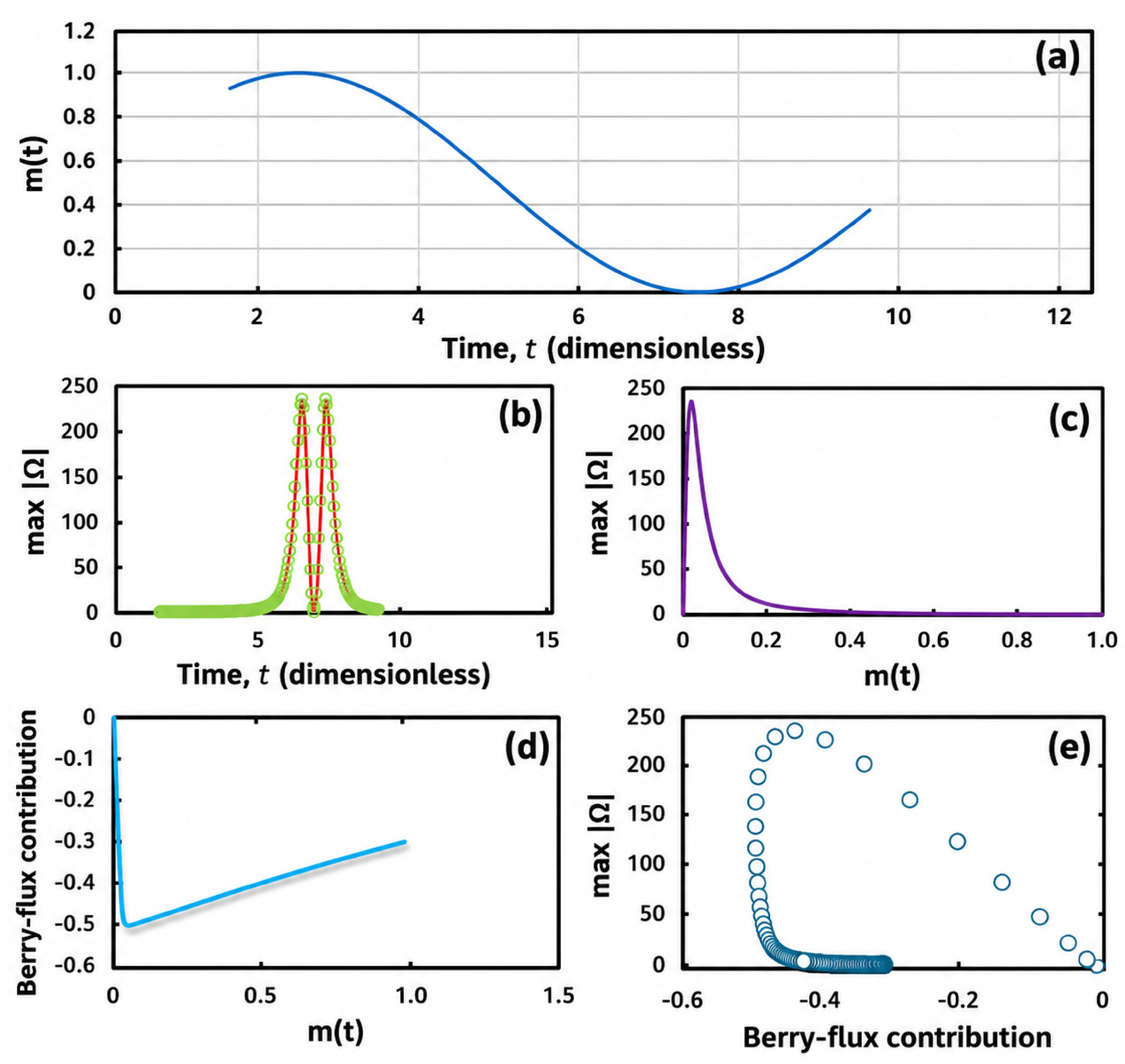
However, the Chern number, which is found by integrating the Berry curvature over all of momentum space, does not change suddenly with each oscillation of . It changes more slowly because it shows the net accumulated curvature over all -points instead of the instantaneous curvature magnitude. In other words, while is very sensitive to changes in the local band-structure variations, the integrated Chern number shows the global topological state of the system. This means that the observed twin peaks in correspond to passing through values close to zero during its oscillation. The smoother modulation of the Chern number, on the other hand, shows how the system’s overall geometric phase structure is changing all the time. The sharp, localized curvature response and the gradual topological evolution work together to create a clear real-time signature of how dynamic mass modulation drives topological phase oscillations in the model. The system changes over time as the mass term oscillates in a sinusoidal pattern, as shown in Figure 5.
Figure 5.
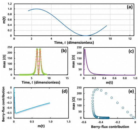
Time-dependent evolution of topological quantities in the driven Dirac model. Time-dependent evolution of geometric quantities in the driven continuum Dirac model. (a) Sinusoidal variation of the mass parameter. (b) Numerically evaluated maximum absolute Berry curvature, illustrating increasing curvature localization as the system approaches the gap-closing region. The finite peak magnitude is resolution dependent and should not be interpreted as the Berry curvature, where the isolated-band Berry curvature is not defined. (c) Dependence of the numerically resolved maximum Berry-curvature magnitude on . (d) Corresponding Berry-flux contribution obtained from integration over the finite momentum-space domain. (e) Parametric relationship between the local curvature magnitude and integrated Berry-flux contribution during mass modulation; time is expressed in normalized dimensionless simulation units because no material-specific dynamical timescale is imposed in the continuum model.
Panel (a) shows that follows a smooth sinusoidal curve, with a peak around s and a lowest point around s. This oscillation periodically moves the system through the critical region ; this is where band inversion and topological transitions can happen. Panel (b) shows how the maximum absolute Berry curvature, , changes over time. It has two peaks next to each other around s. The Berry curvature becomes sharply localized in momentum space when gets close to zero, which is what causes these peaks. This happens when the Dirac Hamiltonian is close to closing a gap.
As the value decreases, the Berry curvature becomes increasingly localized around the Dirac point. For the continuum massive Dirac model, this localization becomes singular in the limit, while at the two bands, it becomes degenerate, and an isolated-band Berry curvature is not well-defined. Consequently, the finite maxima appearing near in the discretized numerical representation should not be interpreted as intrinsic finite physical peaks. Their magnitude and precise location can depend on the momentum-space grid resolution, finite momentum cutoff, and numerical treatment of the gap-closing point. Figure 5 therefore illustrates the concentration of Berry curvature as the system approaches the gap-closing condition rather than assigning a finite Berry-curvature value to the degeneracy itself.
For the lower-band Berry curvature, with the sign depending on convention, has the familiar form:
At k = 0 and m ≠ 0,
Therefore, its magnitude behaves as follows:
which diverges as m → 0 rather than having a physically meaningful finite maximum.
In panel (c), the value of is plotted against the instantaneous mass . Panel (d) shows how the estimated Chern number changes with . The Chern index drops sharply from 0 to about −0.5 around , then slowly rises again; this shows the topological phase inversion as the system moves through the Dirac point. This behavior aligns with the analytical prediction that for the single-valley Dirac model. Finally, panel (e) shows the parametric relationship between the maximum absolute Berry curvature and the estimated Chern index during the time-dependent mass oscillation. Each point represents the instantaneous values of these quantities at a particular stage of mass modulation. As the system approaches the topological transition region, the trajectory initially moves toward more negative Chern estimates (approximately −0.3 to −0.4), accompanied by a pronounced increase in the maximum Berry-curvature amplitude. The curvature subsequently reaches a maximum, indicating a strong local concentration of Berry curvature near the transition. As the mass parameter evolves away from this region, the value progressively decreases toward zero while the Chern estimate follows a different return path. The resulting loop-like parametric trajectory demonstrates that the local Berry-curvature strength and the global topological response do not exhibit a simple one-to-one relationship during dynamic modulation. Rather, their coupled evolution reflects the redistribution of Berry curvature in momentum space as the oscillating mass field drives the system toward and away from the topological transition region.
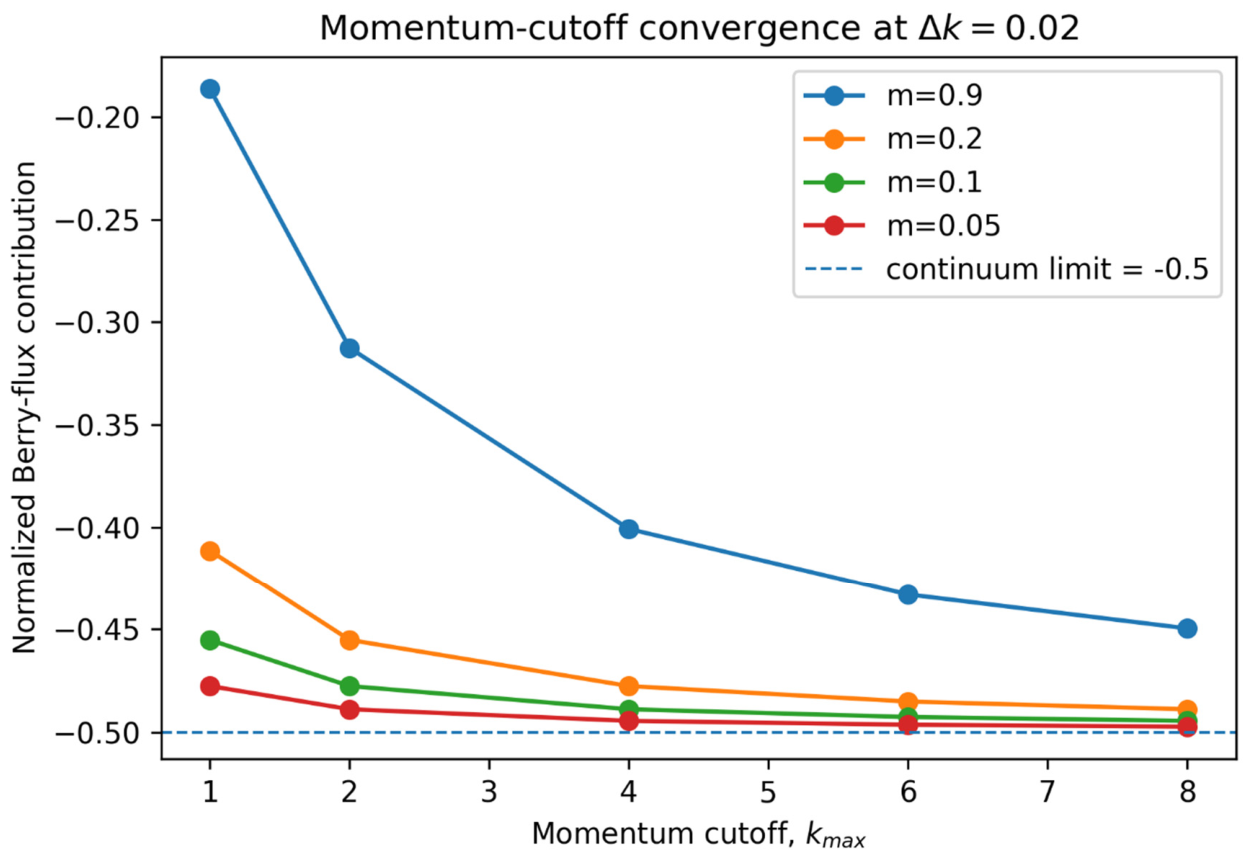
Numerical convergence of the momentum-space integration was examined independently with respect to grid resolution and finite momentum cutoff (see Appendix A). The Berry curvature was evaluated on uniform grids over . At , increasing the grid from to and produced negligible changes in the normalized Berry-flux contribution for representative masses . For example, at , the calculated values were , , and for , , and , respectively. For the more sharply localized case , the result changed from at to at and remained unchanged at , demonstrating convergence after sufficient momentum-space refinement. Cutoff convergence was separately evaluated at fixed ; for , the Berry-flux contribution evolved from at to , , , and for , , , and , respectively, approaching the analytical single-cone limit of . The exact gap-closing point was not assigned to an isolated-band Berry curvature because the two bands are degenerate there.
It is important to clarify that the half-integer value obtained from the present continuum Dirac model represents the Berry-flux contribution of a single massive Dirac cone (or valley), rather than the global Chern invariant of a complete lattice system. Integration of the Berry curvature associated with an isolated continuum Dirac cone over the momentum plane yields a normalized Berry-flux contribution approaching ±1/2, with the sign determined by the mass term and the chosen band convention. This half-integer contribution arises because the single-valley continuum model describes the low-energy region associated with one Dirac cone and does not constitute a complete lattice regularization over the Brillouin zone. In a lattice-regularized system, all relevant valleys and bands must be included over the full Brillouin zone, and their combined contributions yield an integer global Chern number. Accordingly, the quantities calculated from the present continuum model are referred to as Berry-flux contributions (or partial Berry flux), rather than bulk Chern numbers.
It should be emphasized that the instantaneous Berry-curvature peaks observed during the oscillation represent local geometric responses of the evolving band structure and should be distinguished from a rigorously quantized topological invariant. In the present treatment, the Chern estimate is obtained from the instantaneous Berry-curvature distribution and is physically meaningful primarily within the adiabatic or quasi-adiabatic regime, where the system can approximately follow the instantaneous eigenstates. For strongly driven nonadiabatic regimes, a conventional instantaneous Chern number may not adequately characterize the topology, and a full Floquet treatment based on the time-periodic quantum states and quasi-energy spectrum would be required. The present semiclassical model is therefore intended to visualize the evolution of Berry curvature and associated topological tendencies under dynamic mass modulation rather than to provide a complete description of nonadiabatic Floquet topology.
3.5. Coupled Real and Momentum Space Dynamics
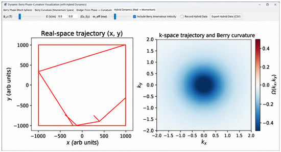
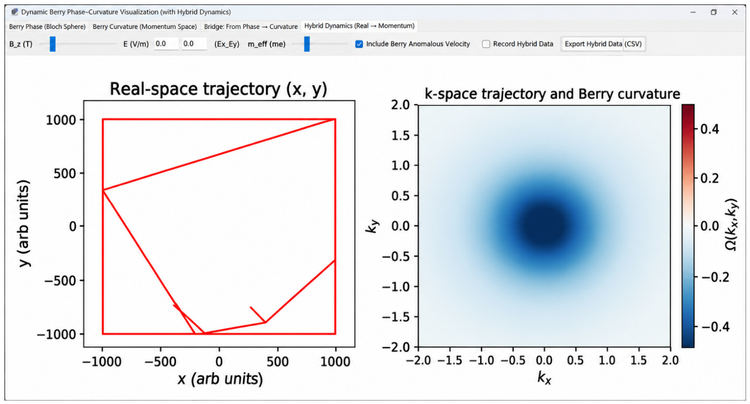
This visualization tab presents side-by-side panels showing the evolution of an electron wavepacket in both real space and momentum space when a magnetic field and topological corrections are applied (see Figure 6). The left panel shows the real-space cyclotron orbit, which changes radius and shape based on the Berry phase and the effective magnetic field.
Figure 6.
Coupled real- and momentum-space dynamics of an electron wavepacket. The left panel shows the real-space cyclotron trajectory, while the right panel displays the corresponding momentum-space (kx–k_y) orbit.
The real-space and momentum-space (kx-ky plane) orbit panels provide illustrative representations of how Berry-curvature-related effects may influence semiclassical transport trajectories. These visualizations are intended to connect the momentum-space geometric quantities with intuitive real-space motion and should not be interpreted as material-specific quantitative transport calculations. In the present implementation, the displayed orbit deformation is used phenomenologically to visualize the expected influence of geometric contributions on semiclassical motion rather than being obtained from a complete self-consistent integration of the coupled semiclassical equations of motion.
For reference, the general semiclassical dynamics of a Bloch wavepacket in the presence of Berry curvature are described by
where is the band energy, is the Berry curvature of band , is the carrier charge, and and are the applied electric and magnetic fields, respectively. The second term in the real-space velocity equation represents the anomalous-velocity contribution. These equations provide the physical basis for the qualitative transport visualization; however, the present orbit panels are not intended as a complete material-specific solution of these coupled equations.
The synchronized animation lets the user directly compare the physical motion of an electron to its evolution in reciprocal space. This shows how the Berry curvature acts like a “momentum-space magnetic field” that subtly distorts trajectories. This dual representation helps show how topological effects connect position and momentum dynamics, offering an intuitive bridge between semiclassical transport and topological band structure.
3.6. Spin Dynamics and Berry Curvature Evolution Under Time-Varying Magnetic Fields
The current advanced simulation framework is built on the previous version of our spin-dynamics visualization tool. It expands the model to include a wider range of time-dependent perturbations and field configurations. This version was made in Python using the Tkinter interface for user-defined parameter control; this lets users choose both the magnetic field and the mass term as arbitrary functions including sinusoidal, exponential, and other analytical forms. This flexibility lets the user look into nonlinear and nonadiabatic regimes where the interaction between spin precession, relaxation, and geometric phase evolution gets complicated.
It should be emphasized that the conventional Berry-phase expression based on instantaneous eigenstates is strictly applicable in the adiabatic limit, where the Hamiltonian varies sufficiently slowly for the evolving quantum state to remain approximately within the corresponding instantaneous eigenstate. When the external field varies rapidly, or when finite relaxation and other dynamical effects become comparable to the driving timescale, this condition may no longer be satisfied. In such nonadiabatic regimes, transitions between instantaneous eigenstates can occur, and the total accumulated phase cannot in general be separated into dynamical and adiabatic geometric contributions using the conventional Berry-phase formula alone. Accordingly, the nonadiabatic and relaxation-dependent trajectories presented in the simulator are used primarily to visualize the evolution of the spin and field configuration, rather than as a rigorous evaluation of an adiabatic Berry phase. A complete treatment of strongly nonadiabatic evolution would require direct time-dependent state evolution and appropriate nonadiabatic geometric-phase formulation.
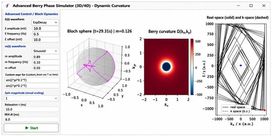
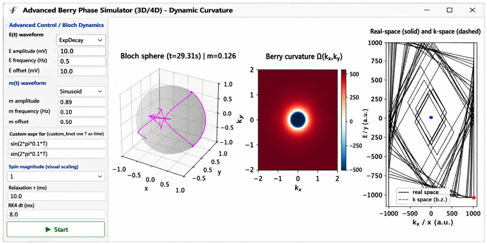
The time evolution of the spin vector is computed using the fourth-order Runge–Kutta (RK4) integration method, chosen because of its numerical stability and accuracy in capturing the fine structure of precession and damping dynamics. The RK4 scheme provides stable numerical integration of the spin-dynamical equations over the adopted parameter range; however, numerical stability of the trajectory does not by itself guarantee the validity of an adiabatic Berry-phase interpretation under rapidly varying fields. The simulation also provides a synchronized depiction of real-space and -space trajectories, with the spin’s motion shown on the Bloch sphere. These elements collectively demonstrate how the changing field configuration modulates the spin vector and induces variations in the Berry curvature , which is recalculated in real time according to the instantaneous mass term . An export feature saves all of the input parameters, instantaneous field values, computed spin trajectories, and curvature data into a structured CSV file so that they can be analyzed further (see Figure 7). In this simulation, the magnetic field was modeled as an oscillatory field that decays exponentially, has an amplitude of 10 mT, a frequency of 0.5 Hz, and a static offset of 10 mT. The magnetic moment was chosen as a sinusoidal function with an amplitude of 0.89 and an offset of 0.5. The relaxation time was set to 10 ms, and the fourth-order Runge–Kutta integration time step was 8 ms. The spin magnitude was normalized to unity. These parameter choices describe a regime in which the magnetic field changes slowly over time, allowing the spin to partially follow the field direction while showing a measurable lag because of finite relaxation. The resulting Bloch-sphere visualization shows a pink arrow that represents the spin vector. At first, it aligns closely with the instantaneous magnetic field direction, but over time it follows a curved path that twists. This twist happens because of the interaction between Larmor precession around and the relaxation term that continuously drives the spin toward . As the magnetic field amplitude decays exponentially, the effective torque on the spin diminishes, resulting in a trajectory that constricts and ultimately converges near the equilibrium direction. The small but finite lag between the spin and the instantaneous field direction produces an additional geometric evolution of the trajectory. Under adiabatic conditions, the corresponding closed-path geometric contribution can be associated with the Berry phase; outside this limit, the trajectory should not be interpreted using the conventional adiabatic Berry-phase expression alone.
Figure 7.
Advanced semiclassical simulator illustrating coupled spin, field, and Berry-curvature dynamics in a time-dependent Dirac system. The Bloch sphere (left) displays the instantaneous orientation of the spin vector S (pink arrow) and its evolution under an oscillating mass term and a decaying magnetic field . The twist-like path covered by S represents the accumulated geometric (Berry) phase. The Berry-curvature map (center) represents , concentrated near , which dynamically fades as increases, representing the modulation of topological behavior and band inversion proximity. Input parameters correspond to = exponential decay (amplitude = 10 mT, offset = 10 mT, frequency = 0.5 Hz) and = sinusoidal (amplitude = 0.89, offset = 0.5). Spin magnitude = 1, relaxation time = 10 ms, and RK4 integration step = 8 ms. The real- and momentum-space orbit panels provide qualitative visualizations of Berry-curvature-related modifications to semiclassical motion; the displayed trajectory deformation is illustrative rather than a material-specific quantitative transport prediction.
The red dot motion in the real-space and -space panels shows how an electron wavepacket evolves in a semiclassical way, where the -space dashed rectangle defines the periodic boundary or sampling region. The red trajectory forming a time-dependent parallelogram shows the influence of the anomalous velocity term , with the vertices of the parallelogram shifting dynamically as changes because of modulation of . The Berry-curvature panel shows the instantaneous curvature distribution . The blue circular region corresponds to strong curvature, which is near . The gradual fading of this feature happens because the time-varying magnetization changes the topological structure of the curvature. When increases, the Berry-curvature magnitude diminishes, and the corresponding visual intensity goes down as well. These input parameters establish a physically coherent dynamical regime where relaxation, precession, and field modulation vie to generate rich spin–field coupling, geometric phase accumulation, and Berry curvature evolution, all of which are crucial for comprehending time-dependent topological magnetization processes.
3.7. Landau Quantization and Berry-Phase–Induced Shift
The Landau-level quantization provides one of the most direct experimental manifestations of geometric phase effects in condensed matter systems. When a charged particle (electron; charge: 1.602 × 10⁻¹⁶ C) moves in a perpendicular magnetic field , its kinetic energy is quantized into discrete Landau levels [16] (LLs),
where is the cyclotron frequency and is the effective mass of the carrier.
In a conventional two-dimensional electron gas (2DEG), the phase offset arises purely from the quantization of orbital motion. However, in systems where the Bloch states carry a Berry phase (such as in topological materials or graphene), the quantization rule is modified according to the Onsager relation [17,18]:
where is the area enclosed by the constant-energy contour in momentum space and
with being the Berry phase accumulated over a cyclotron orbit in -space. For a trivial (non-topological) band, , giving ; for a Dirac system such as graphene, , resulting in . This shift leads to a half-integer quantum Hall effect and directly reflects the topological character of the underlying band structure.
Methodology and Computational Design
To link this theory with the previously discussed Berry-curvature visualizations, the Landau Levels and Quantum Hall tab numerically computes and dynamically visualizes the relationship between magnetic field , effective mass , and the Berry phase . The implementation follows these main steps:
Energy Quantization: For a user-specified effective mass, the Landau levels are computed as
over a range of magnetic field values.
Berry-Phase Correction: The user controls the Bloch-sphere cone angle (from the Berry Phase tab). The corresponding Berry phase is given by where is the solid angle subtended on the Bloch sphere. This value modifies the Onsager quantization parameter [19]:
The Landau-level intersections with the Fermi energy are then adjusted accordingly, demonstrating how the geometric phase shifts the quantization condition.
Onsager Construction: For a chosen Fermi energy , the program calculates the set of magnetic fields satisfying
where and .
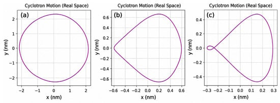
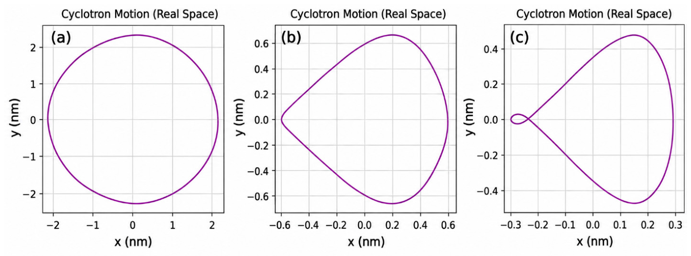
Enabling Berry-phase corrections in the semiclassical simulator produces two coupled effects in the real-space dynamics and quantum spectrum. In real space, the cyclotron orbit deforms from a simple circle into a cone-biased trajectory and, for stronger fields, develops inner epicyclic loops (see Figure 8). This behavior arises because the Berry curvature contributes an anomalous velocity perpendicular to the instantaneous , producing a time-dependent transverse drift. When the magnitude of is comparable to the group velocity, the orbit becomes highly noncircular and can self-intersect. In the energy spectrum, Landau levels scale linearly with (); the substantial increase in observed across the slider range is therefore consistent with the corresponding increase in applied . The Berry phase manifests in the spectrum as an Onsager-like offset (a constant shift of the fan), while its principal dynamical signature in real space is the anomalous, curvature-induced drift that produces the observed orbit distortions. Near parameter regions where is large or band gaps close (e.g., ), semiclassical dynamics may become quantitatively unreliable and full quantum (multiband) calculations are advised.
Figure 8.
Activation of Berry-phase corrections in the semiclassical simulator provides coupled modifications in both the real-space trajectory and the associated quantum spectrum. In real space, the conventional circular cyclotron orbit evolves into a cone-biased, asymmetric path, reflecting the influence of geometric curvature. The trajectory progressively builds complex inner epicyclic loops as the effective magnetic field strength increases, indicating the interaction between orbital dynamics and Berry curvature. The geometric origin of anomalous velocity terms and the consequent topological processes in quantum transport are visually represented by these distortions. The value of the magnetic field: (a) 0.87 T; (b) 3.1 T; and (c) 4.5 T.
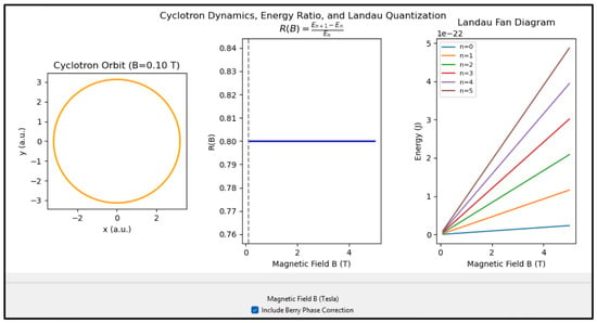
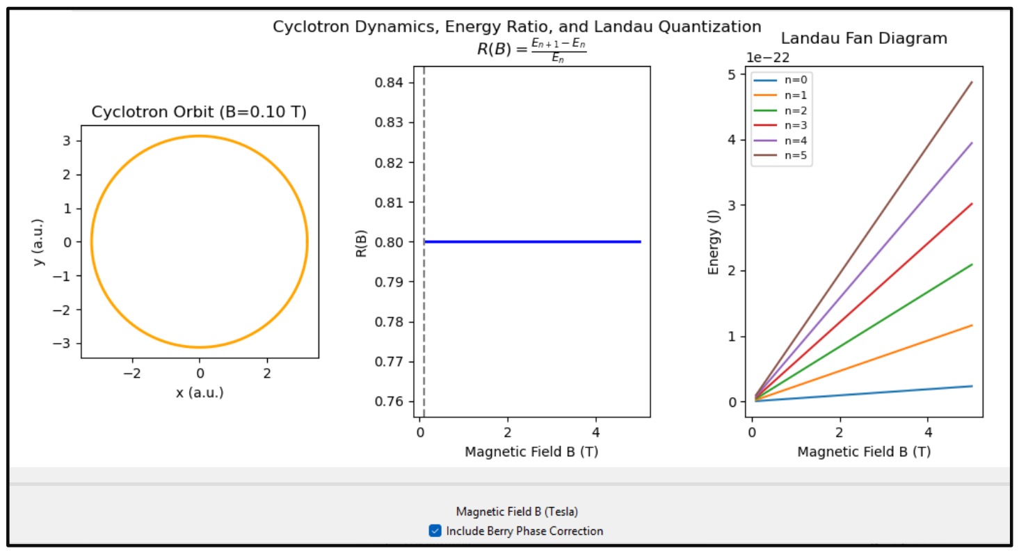
To better understand the relationship between magnetic field strength and cyclotron motion, a simulation module was created to show the evolution of electronic orbits, the energy ratio , and the corresponding Landau fan diagram (see Figure 9). In the present implementation, the cyclotron orbit dynamically deforms as the applied magnetic field changes. This shows the semiclassical trajectory of an electron affected by the Lorentz force and Berry curvature. When the magnetic field is low, the orbit is almost circular. When the magnetic field is high, geometric distortion emerges, forming an asymmetric, cone-like contour as Berry-phase corrections become significant. The calculated ratio remains approximately constant (≈0.8) over the whole field range. This means that, for the chosen effective mass and quantization model, the relative spacing between consecutive Landau levels does not change much with . The Landau fan diagram also shows that energy depends linearly on the magnetic field without a noticeable shift, which is in line with the ideal two-dimensional electron gas model. So, even though the cyclotron orbit visualization shows Berry curvature–induced geometric deformation, the constant and static Landau levels suggest that the underlying quantization stays uniform in this parameter regime. Note that the displayed orbit deformation is phenomenological and is included to qualitatively visualize the possible influence of Berry-phase-related corrections on cyclotron motion; it is not obtained from a self-consistent numerical integration of the complete Berry-curvature-modified semiclassical equations of motion.
Figure 9.
Simulation of magnetic-field-dependent cyclotron motion and quantized energy structure illustrating the interplay between Lorentz dynamics and Berry curvature effects. As the applied magnetic field increases, the initial circular electron orbits gradually deform into asymmetric, cone-like contours, highlighting the geometric influence of the Berry phase on real-space trajectories. The magnetic field was varied from 0.1 to 5.0 T (100 points). Landau levels (n = 1–5) were considered, while R(B) was evaluated at n = 1. Cyclotron trajectories were generated using 400 angular points, with ro = 1/sqrt (B) and a phenomenological orbit-distortion amplitude of 0.1 for visualization of the Berry-related asymmetry. The orbit deformation is shown as an illustrative phenomenological visualization rather than as a material-specific solution of the complete semiclassical transport equations.
4. Discussion
The results collectively demonstrate how Berry-phase phenomena can be explored through complementary real-space, momentum-space, and Bloch-sphere representations within a unified interactive framework. The Bloch-sphere simulations establish the geometric relationship between the enclosed solid angle and accumulated Berry phase, while the continuum Dirac-model calculations extend this visualization to momentum-space Berry curvature and its evolution with the mass parameter. The time-dependent simulations further illustrate how changes in model parameters influence geometric quantities, while the real- and momentum-space trajectory modules provide an intuitive representation of their possible connection with transport behavior. Taken together, these results show the value of combining analytical concepts with interactive numerical visualization for examining geometric effects that are otherwise difficult to interpret from equations alone.
The present framework should, however, be interpreted within the assumptions of the individual models. In particular, the Berry-flux contribution obtained from a single continuum Dirac cone should not be interpreted as the integer global Chern invariant of a complete lattice system, which requires an appropriate lattice regularization and consideration of the full Brillouin zone. Similarly, the displayed transport trajectories are primarily illustrative and are not intended as material-specific solutions of complete semiclassical transport dynamics. Accordingly, unless explicitly identified as physical quantities with specified units, the numerical values, parameter ranges, spatial/temporal scales, and graphical outputs used in the simulations should be regarded as normalized or illustrative model quantities rather than experimentally calibrated material parameters. The framework therefore serves principally as a computational and conceptual platform rather than a quantitative predictor of specific materials or devices. Nevertheless, its modular structure provides a useful basis for future extensions incorporating material-specific parameters, lattice-based Hamiltonians, more complete transport equations, and experimentally relevant conditions.
Within these limitations, the and gap-closing cases are treated according to the assumptions of the continuum model, while the adiabatic and semiclassical results are interpreted only within their respective regimes of validity. Numerical results were additionally checked for convergence with respect to the relevant discretization and computational parameters, and the principal model parameters and their interpretation are specified to facilitate reproducibility. Extensions to non-Abelian or multiband systems would require the corresponding multiband Hamiltonians and geometric formalism, while material- or device-specific predictions would require additional physical parameters and experimental validation beyond the scope of the present work.
5. Conclusions
This study presents an interactive computational visualization framework for investigating Berry-phase phenomena and related geometric effects in quantum systems. A user-controlled simulation environment was developed using Python (v3.11), Tkinter, and Matplotlib to connect theoretical quantum concepts with intuitive, real-time visualizations. The simulator allows users to vary parameters such as magnetic-field orientation, angular frequency, cone angle, and Dirac mass and observe their influence on spin precession, geometric phase accumulation, and momentum-space Berry curvature. The framework integrates complementary modules addressing Bloch-sphere evolution, time-dependent Hamiltonians, momentum-space Berry-curvature mapping, and illustrative real–momentum-space dynamics.
Analytical benchmarks for the underlying models provide reference points for evaluating the numerical implementation, while the interactive framework enables systematic exploration of parameter-dependent geometric behavior. The present simulations are intended primarily for conceptual and computational investigation rather than quantitative prediction of specific materials or devices. In particular, the continuum Dirac model describes Berry-flux contributions from a single Dirac cone rather than a complete lattice-regularized bulk topological invariant, and the illustrative transport trajectories should not be interpreted as material-specific solutions of the complete semiclassical transport equations. Strongly nonadiabatic regimes would likewise require a more complete time-dependent treatment. Nevertheless, the framework provides an accessible connection between geometric quantum concepts and their manifestations in spin and momentum space and may support further exploration of phenomena relevant to quantum materials, spintronics, and topological electronics.
Author Contributions
Conceptualization, P.K.S.; methodology, P.K.S. and R.S.S.; software, P.K.S.; validation, P.K.S., R.S.S. and G.K.; formal analysis, P.K.S.; investigation, P.K.S.; resources, P.K.S. and M.L.F.; data curation, P.K.S.; writing—original draft preparation, P.K.S.; writing—review and editing, P.K.S., R.S.S., M.L.F. and G.K.; visualization, P.K.S.; supervision, P.K.S. and M.L.F.; project administration, P.K.S.; funding acquisition, P.K.S. and M.L.F. All authors have read and agreed to the published version of the manuscript.
Funding
This research received no external funding.
Data Availability Statement
The data supporting the findings of this study are included within the article. The source code used for the simulations and visualizations is openly available through the authors’ GitHub repository. The repository provides the computational framework used to reproduce and further explore the simulations presented in this work. Further inquiries can be directed to the corresponding author. Link for the open-source files: https://github.com/saraswatp/Berry-Phase-Simulations (accessed on the 17 September 2026).
Conflicts of Interest
The authors declare no conflicts of interest.
Appendix A
Figure A1.
Momentum-space grid convergence of the normalized Berry-flux contribution.
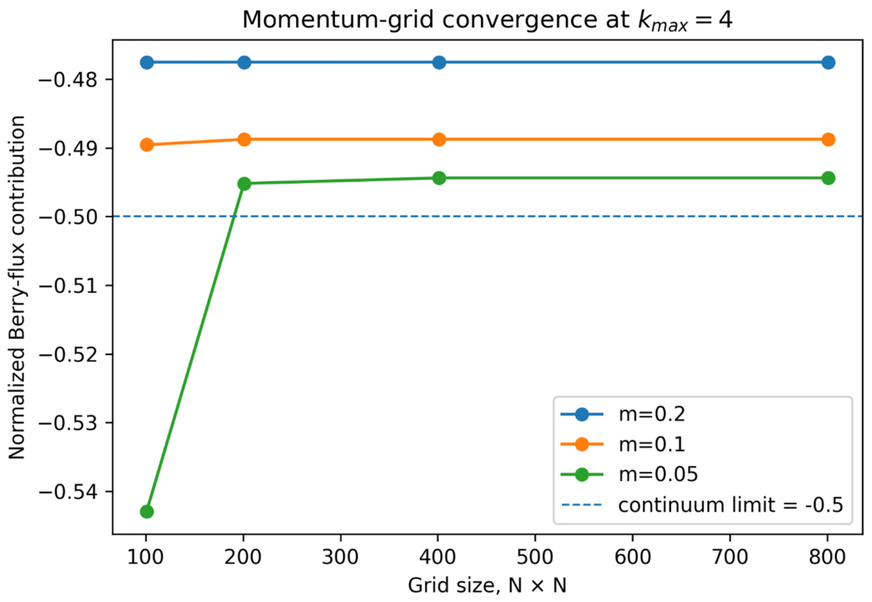
Figure A2.
Momentum-cutoff convergence of the normalized Berry-flux contribution.
References
- Sarswat, P.K.; Sarkar, S.; Yi, G.; Free, M.L. Phosphorus-doped SnTe-type needle-like crystals: Band structure modifications and electronic properties. J. Phys. Chem. C 2017, 121, 18263–18273. [Google Scholar] [CrossRef] [Scilit]
- Moore, J.E. The birth of topological insulators. Nature 2010, 464, 194–198. [Google Scholar] [CrossRef] [Scilit] [PubMed]
- Wang, L.; Troyer, M.; Dai, X. Topological Charge Pumping in a One-Dimensional Optical Lattice. Phys. Rev. Lett. 2013, 111, 026802. [Google Scholar] [CrossRef] [Scilit] [PubMed]
- Xiao, D.; Chang, M.-C.; Niu, Q. Berry phase effects on electronic properties. Rev. Mod. Phys. 2010, 82, 1959–2007. [Google Scholar] [CrossRef] [Scilit]
- Ghahari, F.; Walkup, D.; Gutiérrez, C.; Rodriguez-Nieva, J.F.; Zhao, Y.; Wyrick, J.; Natterer, F.D.; Cullen, W.G.; Watanabe, K.; Taniguchi, T.; et al. An on/off Berry phase switch in circular graphene resonators. Science 2017, 356, 845–849. [Google Scholar] [CrossRef] [Scilit] [PubMed]
- Wu, S.; Ross, J.S.; Liu, G.-B.; Aivazian, G.; Jones, A.; Fei, Z.; Zhu, W.; Xiao, D.; Yao, W.; Cobden, D.; et al. Electrical tuning of valley magnetic moment through symmetry control in bilayer MoS2. Nat. Phys. 2013, 9, 149–153. [Google Scholar] [CrossRef] [Scilit]
- Berry, M.V. Quantal phase factors accompanying adiabatic changes. Proc. R. Soc. London Ser. A Math. Phys. Sci. 1984, 392, 45–57. [Google Scholar] [CrossRef] [Scilit]
- Morinaga, A.; Monma, A.; Honda, K.; Kitano, M. Berry’s phase for a noncyclic rotation of light in a helically wound optical fiber. Phys. Rev. A 2007, 76, 052109. [Google Scholar] [CrossRef] [Scilit][Green Version]
- Hassani Gangaraj, A.; Silveirinha, M.; Hanson, G.W. Berry Phase, Berry Connection, and Chern Number for a Continuum Bianisotropic Material From a Classical Electromagnetics Perspective. IEEE J. Multiscale Multiphysics Comput. Tech. 2017, 2, 3–17. [Google Scholar] [CrossRef] [Scilit]
- Bandyopadhyay, A.; Datta, S.; Jana, D.; Nath, S.; Uddin, M.M. The topology and robustness of two Dirac cones in S-graphene: A tight binding approach. Sci. Rep. 2020, 10, 2502. [Google Scholar] [CrossRef] [Scilit] [PubMed]
- Spanton, E.M.; Zibrov, A.A.; Zhou, H.; Taniguchi, T.; Watanabe, K.; Zaletel, M.P.; Young, A.F. Observation of fractional Chern insulators in a van der Waals heterostructure. Science 2018, 360, 62–66. [Google Scholar] [CrossRef] [Scilit] [PubMed]
- Rudner, M.S.; Song, J.C.W. Self-induced Berry flux and spontaneous non-equilibrium magnetism. Nat. Phys. 2019, 15, 1017–1021. [Google Scholar] [CrossRef] [Scilit]
- Gaikwad, A.; Sun, S.; Wang, P.; Zhang, L.; Cano, J.; Dai, X.; Du, X. Strain-tuned topological phase transition and unconventional Zeeman effect in ZrTe5 microcrystals. Commun. Mater. 2022, 3, 94. [Google Scholar] [CrossRef] [Scilit]
- Wright, A.R.; McKenzie, R.H. Quantum oscillations and Berry’s phase in topological insulator surface states with broken particle-hole symmetry. Phys. Rev. B 2013, 87, 085411. [Google Scholar] [CrossRef] [Scilit]
- Mitsuishi, N.; Sugita, Y.; Bahramy, M.S.; Kamitani, M.; Sonobe, T.; Sakano, M.; Shimojima, T.; Takahashi, H.; Sakai, H.; Horiba, K.; et al. Switching of band inversion and topological surface states by charge density wave. Nat. Commun. 2020, 11, 2466. [Google Scholar] [CrossRef] [Scilit] [PubMed]
- Fürst, M.; Kochan, D.; Dusa, I.-G.; Gorini, C.; Richter, K. Dirac Landau levels for surfaces with constant negative curvature. Phys. Rev. B 2024, 109, 195433. [Google Scholar] [CrossRef] [Scilit]
- Onsager, L. Interpretation of the de Haas-van Alphen effect. Lond. Edinb. Dublin Philos. Mag. J. Sci. 1952, 43, 1006–1008. [Google Scholar] [CrossRef] [Scilit]
- Mikitik, G.P.; Sharlai, Y.V. Manifestation of Berry’s Phase in Metal Physics. Phys. Rev. Lett. 1999, 82, 2147–2150. [Google Scholar] [CrossRef] [Scilit]
- Babaev, E.; Ashcroft, N.W. Violation of the London law and Onsager–Feynman quantization in multicomponent superconductors. Nat. Phys. 2007, 3, 530–533. [Google Scholar] [CrossRef] [Scilit]

Disclaimer/Publisher’s Note: The statements, opinions and data contained in all publications are solely those of the individual author(s) and contributor(s) and not of MDPI and/or the editor(s). MDPI and/or the editor(s) disclaim responsibility for any injury to people or property resulting from any ideas, methods, instructions or products referred to in the content. |
© 2026 by the authors. Licensee MDPI, Basel, Switzerland. This article is an open access article distributed under the terms and conditions of the Creative Commons Attribution (CC BY) license.