Spin Spiral vs. Spin Stripe in La_2−xBa_xCuO₄ (x = $\frac{1}{8}$): Analysis of μSR Data

Abstract

There are two models that explain the incommensurate elastic neutron scattering from ${\mathrm{La}}_{2-x}{\mathrm{Ba}}_x{\mathrm{CuO}}_4$ ($x={\displaystyle \frac{1}{8}}$), (i) spin spiral and (ii) collinear spin stripe. I show that available $\mu$SR data taken with a polycrystalline sample is consistent with the generic (arbitrary parameters) coplanar spin spiral. On the other hand for consistency with the collinear spin stripe one needs fine tuning of the parameters of the model. I also propose a further $\mu$SR experiment with a single crystal aimed specifically at the window of parameters where the spin stripe model is still consistent with the data. In the proposed experiment, the expected signals for these two models are dramatically different. Such an experiment would finally reject one of the models.

1. Introduction

It is well established that incommensurate magnetic neutron scattering is a generic phenomenon in cuprate superconductors. All cuprate families originate from parent Mott insulators that are collinear antiferromagnets (AFs) with spin S = 1/2. In neutron scattering, the antiferromagnetism is observed as an elastic peak at the momentum transfer $Q=(\pi /a,\pi /a)$, where a is the 2D lattice spacing of the ${\mathrm{CuO}}_2$ plane. The compounds become conducting and ultimately superconducting with doping by holes or electrons. With doping by holes, the neutron scattering peak is shifted from its AF position by an amount q. This is the experimental manifestation of the spin structure generally incommensurate with the crystal lattice. This phenomenon had been observed in single-layer cuprates ${\mathrm{La}}_{1.875}{\mathrm{Ba}}_{0.125}{\mathrm{CuO}}_4$ (LBCO) (Refs. [1,2]) and ${\mathrm{La}}_{2-x}{\mathrm{Sr}}_x{\mathrm{CuO}}_4$ (LSCO) (Refs. [3,4]), in double-layer YBCO (Refs. [5,6]), and in other cuprates. The incommensurate scattering can be elastic/quasielastic [1,2,3,4,6] or fully dynamic [5]. In single-layer cuprates LBSO and LSCO, the incommensurate wave vector q scales linearly with doping x, $q={\displaystyle \frac{2\pi }{a}}x$, for $x<0.16$ (Yamada plot, Ref. [4]). The compound ${\mathrm{La}}_{1.875}{\mathrm{Ba}}_{0.125}{\mathrm{CuO}}_4$ plays a special role. In this case, $x=1/8$; hence, a generally incommensurate spin structure becomes commensurate and in Low-Temperature Tetragonal (LTT) phase spins are pinned to the lattice. The pinning reduces fluctuations and hence enhances the static electron spin. Hence, the electron spin structure can be investigated via muon spin depolarization, $\mu$SR. In this work, I reanalyze $\mu$SR data [7] for polycrystalline ${\mathrm{La}}_{1.875}{\mathrm{Ba}}_{0.125}{\mathrm{CuO}}_4$ to shed light on the spin structure of underdoped cuprates. Let us stress again that ${\mathrm{La}}_{1.875}{\mathrm{Ba}}_{0.125}{\mathrm{CuO}}_4$ plays a special role because spin quantum fluctuations are suppressed due to the LTT phase, and this makes the static spin structure significant. For example, in ${\mathrm{La}}_{1.875}{\mathrm{Sr}}_{0.125}{\mathrm{CuO}}_4$, neutron scattering also manifests incommensurate peaks with same periodicity. However, the peaks are almost inelastic and this implies that there is practically no static magnetic field that can be probed by $\mu$SR. To avoid misunderstanding, it should be noted that at very low temperatures there are small static magnetic moments in ${\mathrm{La}}_{1.875}{\mathrm{Sr}}_{0.125}{\mathrm{CuO}}_4$ and this is reflected in the NMR wipeout. There is an interesting experiment [8] where the superconducting stiffness of ${\mathrm{La}}_{1.875}{\mathrm{Sr}}_{0.125}{\mathrm{CuO}}_4$ has been measured using $\mu$SR depolarization. However, this is $\mu$SR in an external applied magnetic field, not in the intrinsic field of the material.

NMR studies of the magnetic structure are hindered by the wipeout phenomenon; at low temperatures the NMR signal disappears; see, e.g., Ref. [9]. So, NMR just indicates a presence of some static magnetic structure.

The problem of the incommensurate magnetic structure is important purely phenomenologically. However, it also has a deep fundamental importance. The point is that strong coupling theories of the pseudogap phase based on the picture of doped Mott insulator (small hole pockets) necessarily result in the coplanar spin spiral state, see e.g., Ref. [10] On the other hand, weak coupling theories based on the Landau Fermi liquid model with large Fermi surface allow both collinear spin stripes and coplanar spin spirals; see, e.g., Refs. [11,12]. Hence, the spin structure sheds light on nature of the pseudogap state.

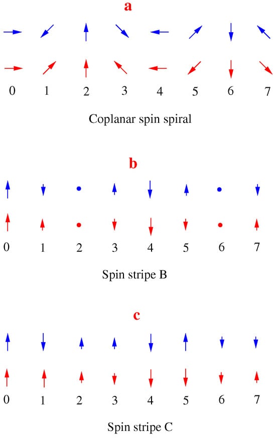
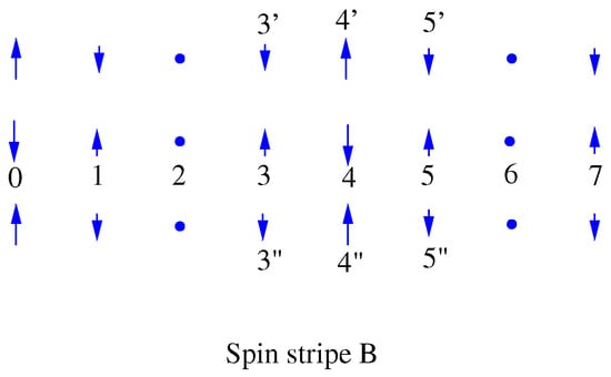
There are two alternative ways to explain the incommensurate spin structure: (i) the coplanar spin spiral and (ii) the spin stripe. In Figure 1, I show different spin patterns: blue arrows in the top line of each panel show real spins and red arrows in the bottom line of each panel show the same in terms of staggered spins; every second spin is flipped upside down to exclude trivial antiferromagnetic ordering. The incommensurate structure is visually more transparent in terms of the staggered spins. Below, I mostly use the staggered notations. Equations describing the amplitude and the direction of the static component of the staggered spin are

$$\begin{array}{ccc}& & spiral:\mathbf{S}\propto \widehat{\mathbf{x}}cos\left(qx\right)+\widehat{\mathbf{y}}sin\left(qx\right)\hfill \\ & & stripe:\mathbf{S}\propto \widehat{\mathbf{x}}cos(qx+\phi )\hfill \end{array}$$

(1)

In the case of stripes, there are always higher Fourier harmonics, but theoretically they are usually small; see, e.g., Ref. [12]. However, there are also works where higher harmonics are significant [11]. The coplanar spin spiral for $q=2\pi /8$ is shown in panel a of Figure 1.

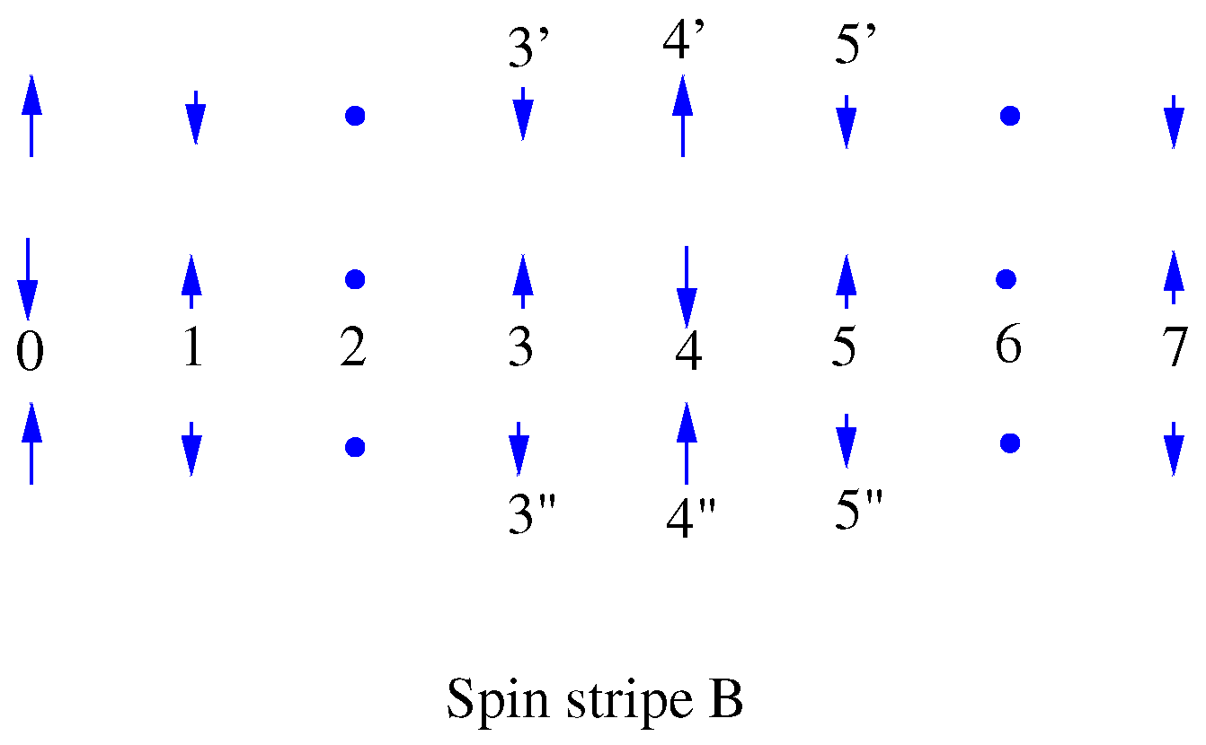
Figure 1. The spin spiral and different types of spin stripes; the numbers enumerate lattice sites. Blue arrows show real spins and red arrows show the same in terms of staggered spins (every second spin is flipped upside down). (a) Coplanar spin spiral; (b) Spin stripe B; (c) Spin stripe C.

The spin stripe for $q=2\pi /8$ and $\phi =0$,

$$\begin{array}{c}\hfill S_n\propto cos\left({\displaystyle \frac{2\pi n}{8}}\right),n=0,1,2,3,4,5,6,7\end{array}$$

(2)

is shown in panel b of Figure 1. I call it “spin stripe B”. This is the most commonly considered type of the spin stripe. For completeness I also consider the spin stripe with $q=2\pi /8$ and $\phi =-\pi /8$,

$$S_n\propto cos\left({\displaystyle \frac{2\pi n}{8}}-\pi /8\right),n=0,1,2,3,4,5,6,7$$

(3)

The corresponding picture is shown in panel c of Figure 1. I call it “spin stripe C”. It is worth stressing that case C is interesting only theoretically; in the literature, “spin stripe” is practically always case B.

It is important to note that muons stop at the apical oxygens; see, e.g., Refs. [13,14]. Therefore, the depolarization rate is directly proportional to the static electron spin located on Cu ion straight underneath the apical oxygen.

2. Spin Spiral

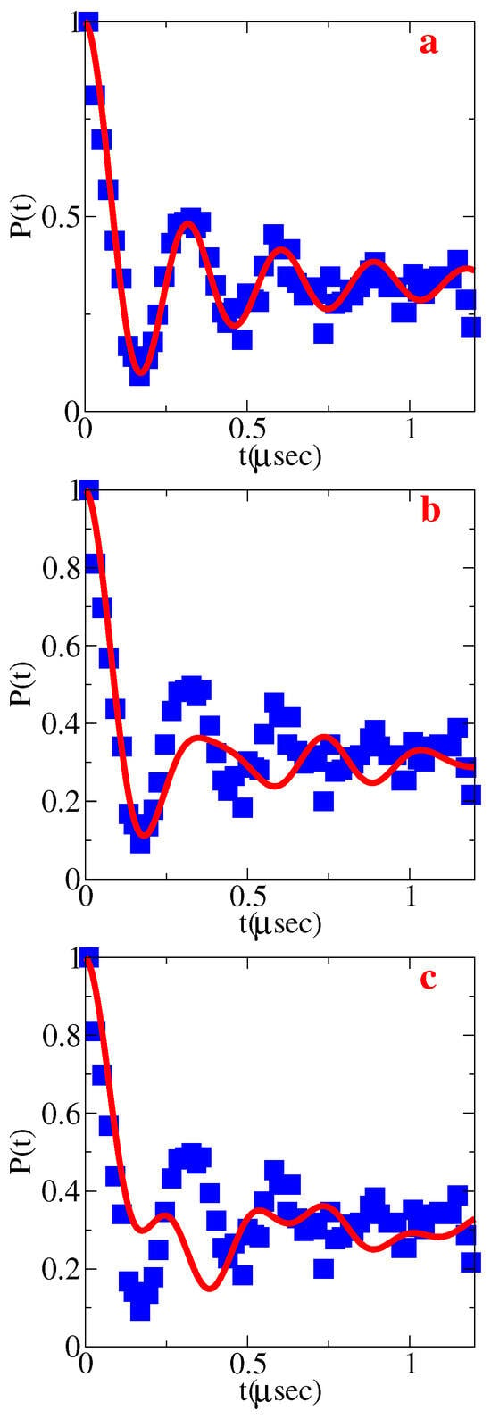
$\mu$SR data (muon polarization versus time) for polycrystalline ${\mathrm{La}}_{2-x}{\mathrm{Ba}}_x{\mathrm{CuO}}_4$ ($x={\displaystyle \frac{1}{8}}$) from Ref. [7] are presented in Figure 2 by blue squares. The blue squares in all three panels, a, b, and c, are identical. First I fit the data assuming a single depolarization magnetic field and using the same formula as that used in the original experimental work [7].

$$\begin{array}{c}\hfill P\left(t\right)={\displaystyle \frac{V_m}{3}}\left[2e^{-{\lambda }_{T}t}{J}_0\left(\omega t\right)+e^{-{\lambda }_{L}t}\right]+(1-V_m)e^{-{\lambda }_{nm}t}\end{array}$$

(4)

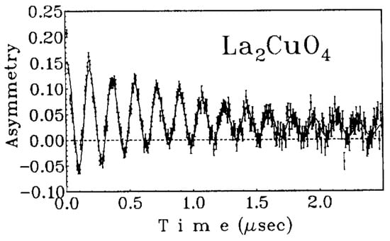
Here, $\omega =2{\mu }_{\mu }{B}_d$, ${\mu }_{\mu }$ is magnetic moment of muon and $B_d$ is the depolarizing field due to the electron spin; ${\lambda }_T, {\lambda }_L, {\lambda }_{nm}$ are various relaxation rates; and $V_m$ is the relative fraction of muons that stopped at the sites sensitive to B (stopped at apical oxygens). It is worth noting that the fitting formula for $P\left(t\right)$ comes from averaging the on-site simple cosine depolarization rate [15] over directions of the on-site magnetic field in the polycrystalline sample. Of course, the exact polycrystalline sample disorder is not known; therefore, Equation (4) is semiphenomenological. It works remarkably well: the fingerprint for the Bessel function is the ratio of heights of different maxima. It is also worth noting that in the parent ${\mathrm{La}}_2{\mathrm{CuO}}_4$ polycrystalline sample [16], the $\mu$SR signal is closer to simple cosine; see Figure 3. Practically, for fitting properties, Equation (4) can be simplified as

$$\begin{array}{c}\hfill P\left(t\right)=U_m{e}^{-{\lambda }_{T}t}{J}_0\left(\omega t\right)+(1-U_m)e^{-{\lambda }^{\prime }t}\end{array}$$

(5)

Moreover, for the fit within the relevant time range $0<t<1.2$ μs, I set ${\lambda }^{\prime }=0$, because practically it does not influence the fits. The fit of the data gives the following parameters: $\omega =22\times {10}^6{\mathrm{s}}^{-1}$, ${\lambda }_T=0.9\times {10}^6{\mathrm{s}}^{-1}$, $U_m=0.67$. This results in the red solid curve in panel a of Figure 2 being practically identical to the fit in Ref. [7]. Agreement with data is excellent.

Figure 2. Muon polarization vs. time. Blue squares in all panels show T = 5K data from Ref. [7]. The red curve in panel (a) shows the best fit of data in the spin spiral model. The red curve in panel (b) shows the best fit of data in the “spin stripe B” model. The red curve in panel (c) shows the best fit of data in the “spin stripe C” model.

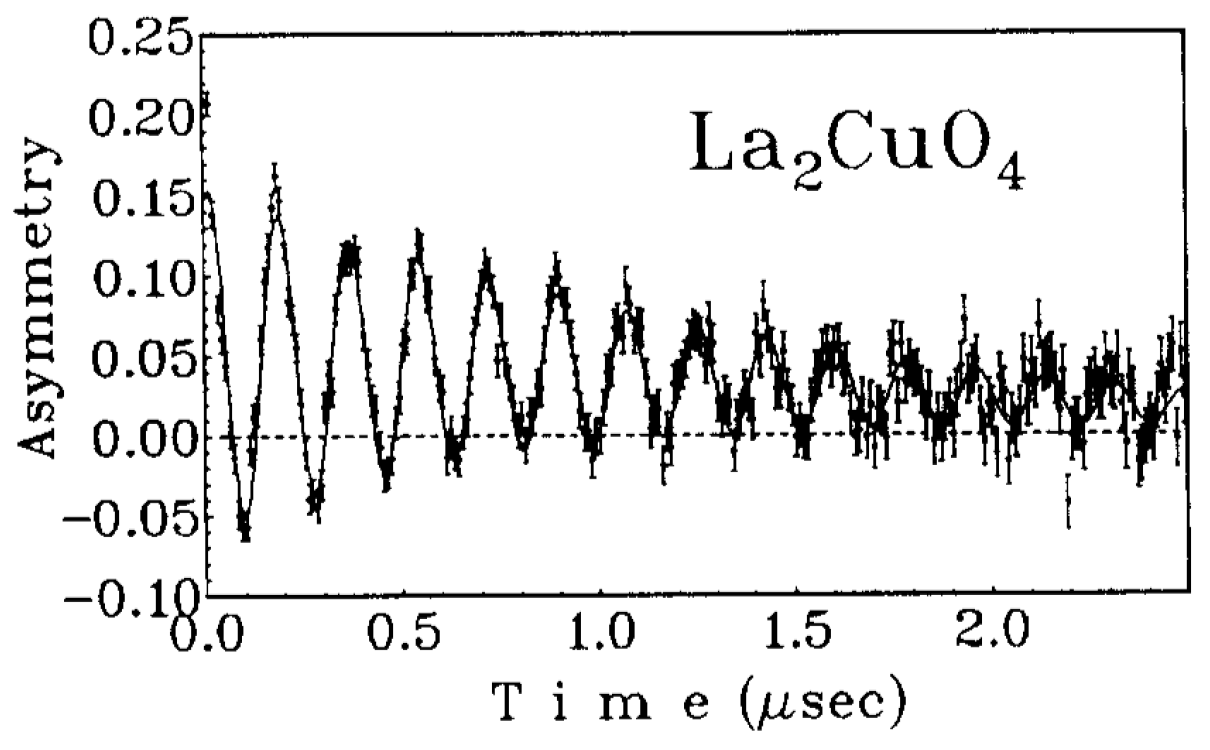
Figure 3. Muon spin depolarization in parent ${\mathrm{La}}_2{\mathrm{CuO}}_4$, Ref. [16].

The fit with Equation (4) or Equation (5) assumes a single depolarization magnetic field with random directions of the field related to the polycrystal. The muon sensitive to the magnetic moment of Cu is located on the apical oxygen. Therefore, the single depolarization field implies that magnetic moments at all sites are the same. We also know from neutron scattering that there is an antiferromagnetic structure with period 8 lattice spacing. Therefore, the single depolarization field calculation is consistent with the spin spiral shown in Figure 1. Moreover, the plane of the spiral must coincide with the ${\mathrm{CuO}}_2$ plane; otherwise, the depolarization rate at different sites would be different.

Figure 3 shows $\mu$SR depolarization data [16] in the parent ${\mathrm{La}}_2{\mathrm{CuO}}_4$. Fitting with $cos\left(\omega t\right)$, the depolarization gives $\omega =36\times {10}^6{\mathrm{s}}^{-1}$. This has to be compared with $\omega =22\times {10}^6{\mathrm{s}}^{-1}$ obtained for ${\mathrm{La}}_{1.875}{\mathrm{Ba}}_{0.125}{\mathrm{CuO}}_4$. It is known that the electron magnetic moment in ${\mathrm{La}}_2{\mathrm{CuO}}_4$ is ${\mu }_e=(0.6\pm 0.05){\mu }_B$ (Ref. [17]). Hence, the electron magnetic moment in ${\mathrm{La}}_{1.875}{\mathrm{Ba}}_{0.125}{\mathrm{CuO}}_4$ is

$$\begin{array}{c}\hfill {\mu }_e={\displaystyle \frac{22}{36}}\times 0.6{\mu }_B=0.37{\mu }_B.\end{array}$$

(6)

This implies that spin fluctuations are very strong. Already in the parent ${\mathrm{La}}_2{\mathrm{CuO}}_4$ the fluctuations reduce the static spin as $1/2\to 0.3$. In ${\mathrm{La}}_{1.875}{\mathrm{Ba}}_{0.125}{\mathrm{CuO}}_4$, the reduction is even more significant, $1/2\to 0.18$.

3. Spin Stripe B Model

In the spin stripe B, described in Figure 1b and Equation (2), the depolarizing magnetic field is different at different sites. Within one period, say sites 2, 3, 4, and 5 in Figure 1b, the depolarizing field is maximum at site 4, while at sites 3 and 5 it is smaller by a factor of $1/\sqrt{2}$, and there is no depolarization at site 2. Therefore, to describe the muon spin depolarization one has to perform the following replacement in Equations (4) and (5)

$$\begin{array}{ccc}\hfill J_0\left(\omega t\right)& \to & {\displaystyle \frac{1}{3}}[J_0\left(\omega t\right)+2J_0\left(p\omega t\right)]\hfill \\ \hfill p& =& 1/\sqrt{2}=0.71\hfill \end{array}$$

(7)

Here, $\omega$ corresponds to depolarization at sites n = 0, 4. The time dependence is the combination of the Bessel functions because the polycrystalline orientation averaging is independent of the site. The best fit achieved at $\omega =26\times {10}^6{\mathrm{s}}^{-1}$, ${\lambda }_T=1.0\times {10}^6{\mathrm{s}}^{-1}$, $U_m=0.7$ is shown by a solid red line in panel b of Figure 2. The fit is not consistent with the data. This rules out the spin stripe B model.

4. Spin Stripe C Model

In the spin stripe C, described by Figure 1c and Equation (3), the depolarizing magnetic field is also different at different sites. Within one period, say sites 2, 3, 4, and 5 in Figure 1c, the depolarizing field is maximum at sites 4 and 5, and at sites 2 and 3 it is smaller by a factor of $cos(3\pi /8)/cos(\pi /8)$. Therefore, to describe the muon spin depolarization one has to perform the following replacement in Equations (4) and (5):

$$\begin{array}{ccc}\hfill J_0\left(\omega t\right)& \to & {\displaystyle \frac{1}{2}}[J_0\left(\omega t\right)+J_0\left(p\omega t\right)]\hfill \\ \hfill p& =& {\displaystyle \frac{cos(3\pi /8)}{cos(\pi /8)}}=0.41\hfill \end{array}$$

(8)

Here, $\omega$ corresponds to relaxation at sites n = 0, 1, 4, 5. The best fit achieved at $\omega =26\times {10}^6{\mathrm{s}}^{-1}$, ${\lambda }_T=1.0\times {10}^6{\mathrm{s}}^{-1}$, $U_m=0.7$ is shown by the solid red line in panel c of Figure 2. The fit is inconsistent with the data. This rules out the “spin stripe C” model.

Inconsistency with data is a general situation with the harmonic spin stripe model. For example, for $\phi =-\pi /16$ in (1), there are four different depolarization frequencies $0.98:0.83:0.20:0.55$ and the relaxation curve has nothing in common with the data.

5. Modified Spin Stripe B Model

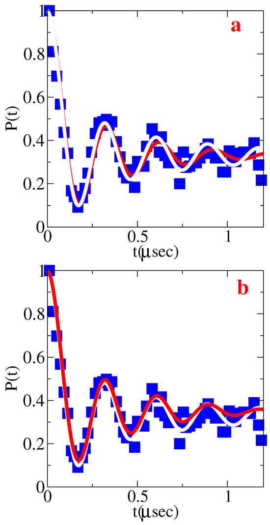
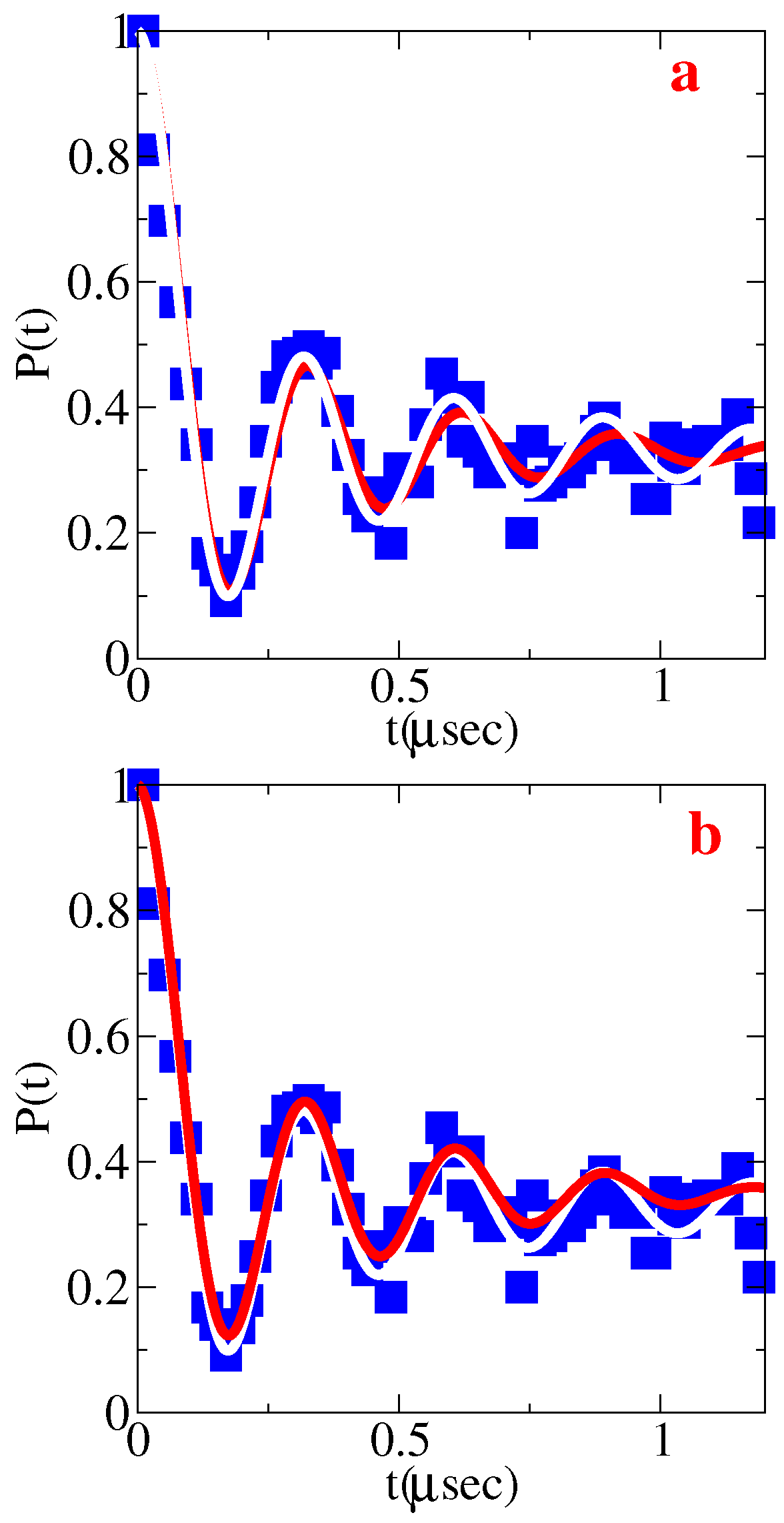
The spin stripe B that has nodes is the most popular model; see, e.g., Ref. [11]. In principle, the spin stripe can be anharmonic. Actually, the initial spin stripe model suggested ad hoc was strongly unharmonic, $p=1$, and early theoretical calculations supported this model [11]. However, more recent calculations favor the harmonic collinear spin stripe [12]. Anyway, let us consider an anharmonic modification of spin stripe B model. The shape is like that in Figure 1b, but the ratio of the small spin over the large spin, $p=|S_1|/|S_0|$, is arbitrary instead of $p=1/\sqrt{2}$. What range of the ratio is consistent with the data? In panel a of Figure 4, the red line presents the best fit for $p=0.9$ (the fitting parameters are $\omega =23\times {10}^6{\mathrm{s}}^{-1}$, ${\lambda }_T=1.0\times {10}^6{\mathrm{s}}^{-1}$, $U_m=0.67$). For comparison, the white line represents the fit at $p=1$ that is identical to the spin spiral fit shown by the red line in Figure 2a. The red fit is not bad, but it is still moving out of the phase compared to the data at large t. At $p=0.95$, the “modified spin stripe B” model becomes consistent with $\mu$SR data. Hence, the range consistent with data is $0.95\le p\le 1.05$.

Figure 4. Muon polarization vs. time. Blue squares show T=5K data from Ref. [7]. Panel (a): The red curve shows the best fit of the data with the “modified spin stripe B” model at $p=0.9$. Panel (b): The red curve shows the best fit of the data with the “modified spin stripe C” model at $p=0.9$. The white line in both panels represents the fit at $p=1$ that is identical to the spin spiral fit shown by the red line in Figure 2a.

6. Modified Spin Stripe C Model

Finally let us consider a modification of the spin stripe C model: the shape is like that in Figure 1c but the ratio of the small spin over the large spin, $p=|S_2|/|S_1|$, is arbitrary instead of $p={\displaystyle \frac{cos(3\pi /8)}{cos(\pi /8)}}=0.41$. In panel b of Figure 4, the red line presents the best fit for $p=0.9$ (the fitting parameters are $\omega =23\times {10}^6{\mathrm{s}}^{-1}$, ${\lambda }_T=0.7\times {10}^6{\mathrm{s}}^{-1}$, $U_m=0.65$). Again, for comparison, the white line represents the fit at $p=1$ that is identical to the spin spiral fit shown by the red line in Figure 2a. The red fit is not bad, but it is still somewhat far from the data at large t. At $p=0.95$, the “modified spin stripe C” model becomes consistent with $\mu$SR data. Hence, again, the range consistent with the experiment is $0.95\le p\le 1.05$.

7. Effect of Nearest Neighbors in the Modified Spin Stripe Model B

In the analysis up to this point I assumed that the muon stopped at the apical oxygen is sensitive only to the magnetic field of the Cu ion underneath. However, the contribution of nearest-neighbor Cu ions to the depolarizing field while being small is not quite negligible. In the case of the spin spiral, this additional contribution does not change anything. Consistently with $\mu$SR data, the depolarizing magnetic field at each apical oxygen is the same even when taking into account all neighbors.

However, in the case of the spin stripe, the additional depolarization slightly influences the analysis. Let us consider the modified spin stripe B that is mostly accepted in the literature. Figure 5 shows the spin arrangement in the spin stripe.

Figure 5. Spin stripe B, the same as that in Figure 1b. However, here I show the square lattice and also the real spins (not staggered).

The magnetic field of an electron with magnetic moment $\mathit{M}$ is given by the dipole formula

$$\begin{array}{c}\hfill \mathit{B}={\displaystyle \frac{3\widehat{\mathit{r}}(\mathit{M}·\widehat{\mathit{r}})-\mathit{M}}{r^3}}\end{array}$$

(9)

Hence, the depolarizing magnetic field at the apical oxygen above site 4 considering the nearest-neighbor spins 3, 5, $4^{\prime }$, $4^{″}$ is

$$\begin{array}{ccc}\hfill B_4^{\left(dep\right)}& \propto & {\displaystyle \frac{1}{b^3}}+2{\displaystyle \frac{3a^2/R^2-1}{R^3}}+2{\displaystyle \frac{p}{R^3}}\hfill \\ & \to & 1+2{\displaystyle \frac{b^3}{R^3}}\left({\displaystyle \frac{3a^2}{R^2}}-1\right)-2p{\displaystyle \frac{b^3}{R^3}}\hfill \end{array}$$

(10)

Here, $a=3.8$ is the in-plane lattice spacing, $b=2.5$ is the copper to apical oxygen distance, and $R=\sqrt{a^2+b^2}$. As before, $p=|S_3|/|S_4|$. The first term in (10) comes from the spin at site 4, the second term comes from spins at sites $4^{\prime }$ and $4^{″}$, and the third term comes from spins at sites 3 and 5. The first term has already been accounted for in the analysis above. Now I account for the correction that comes from the second and the third terms.

Similarly, the depolarizing magnetic field at the apical oxygen above site 3 considering the nearest-neighbor spins 4, $3^{\prime }$, and $3^{″}$ is

$$\begin{array}{ccc}\hfill B_3^{\left(dep\right)}& \propto & -{\displaystyle \frac{p}{b^3}}-2p{\displaystyle \frac{3a^2/R^2-1}{R^3}}+{\displaystyle \frac{p}{R^3}}\hfill \\ & \to & p\left[1+2{\displaystyle \frac{b^3}{R^3}}\left({\displaystyle \frac{3a^2}{R^2}}-1\right)\right]-{\displaystyle \frac{b^3}{R^3}}\hfill \end{array}$$

(11)

Here, the first term comes from the spin at site 3, the second term comes from spins at sites $3^{\prime }$ and $3^{″}$, and the third term comes from the spin at site 4. The first term has already been accounted for in the analysis above. Now I account for the correction that comes from the the second and the third terms.

According to $\mu$SR data, the depolarizing fields are equal, $|B_3^{\left(dep\right)}|=|B_4^{\left(dep\right)}|$; solving this equation together with (10) and (11), one finds $p=0.90$. Considering more distant neighbors changes the value of p by less than 1%. Taking into account the error bars discussed above, $p=0.90\pm 0.05$.

To summarize, while the spin spiral naturally explains the equality of the depolarizing fields, the modified spin stripe requires a fine tuning of the spin ratio at different sites. In principle, this is possible: one cannot exclude such a possibility based on existing data. To resolve the issue, the next section suggests a $\mu$SR tomography experiment.

8. $\mathit{\mu }$SR Tomography of the Spin Structure

The experiment that I have been analyzing above has been performed with a polycrystalline sample. Here, I propose a $\mu$SR experiment with a single crystal and use the direction of the initial polarization of the muon as a probe that allows one to distinguish the spin structures.

Consider first the case when the initial muon polarization is orthogonal to ${\mathrm{CuO}}_2$ planes. In both the coplanar spin spiral and the collinear spin stripe, electronic spins are in the ${\mathrm{CuO}}_2$ plane. Therefore, the depolarization in both cases is (see Ref. [15])

$$\begin{array}{c}\hfill P\left(t\right)=U_m{e}^{-{\lambda }_{T}t}cos\left(\omega t\right)+(1-U_m)\end{array}$$

(12)

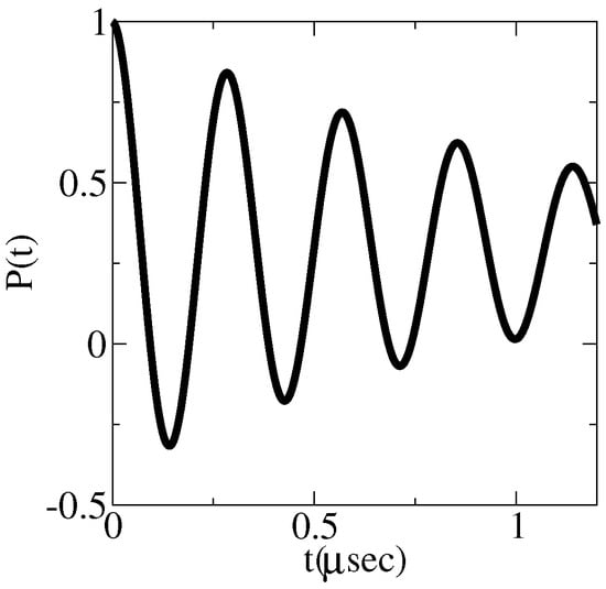
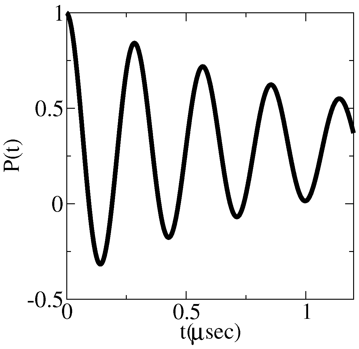
Figure 6 presents the depolarization plot for values $\omega =22\times {10}^6{\mathrm{s}}^{-1}$ and ${\lambda }_T=0.9\times {10}^6{\mathrm{s}}^{-1}$ determined above. I rather arbitrarily set $U_m=0.7$. Hence, depolarization of muons orthogonal to the ${\mathrm{CuO}}_2$ planes does not distinguish the spin patterns under discussion.

Figure 6. Depolarization plot for initial muon polarization perpendicular to ${\mathrm{CuO}}_2$ plane. The plot is the same for the coplanar spin spiral and for the collinear spin stripe.

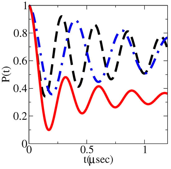
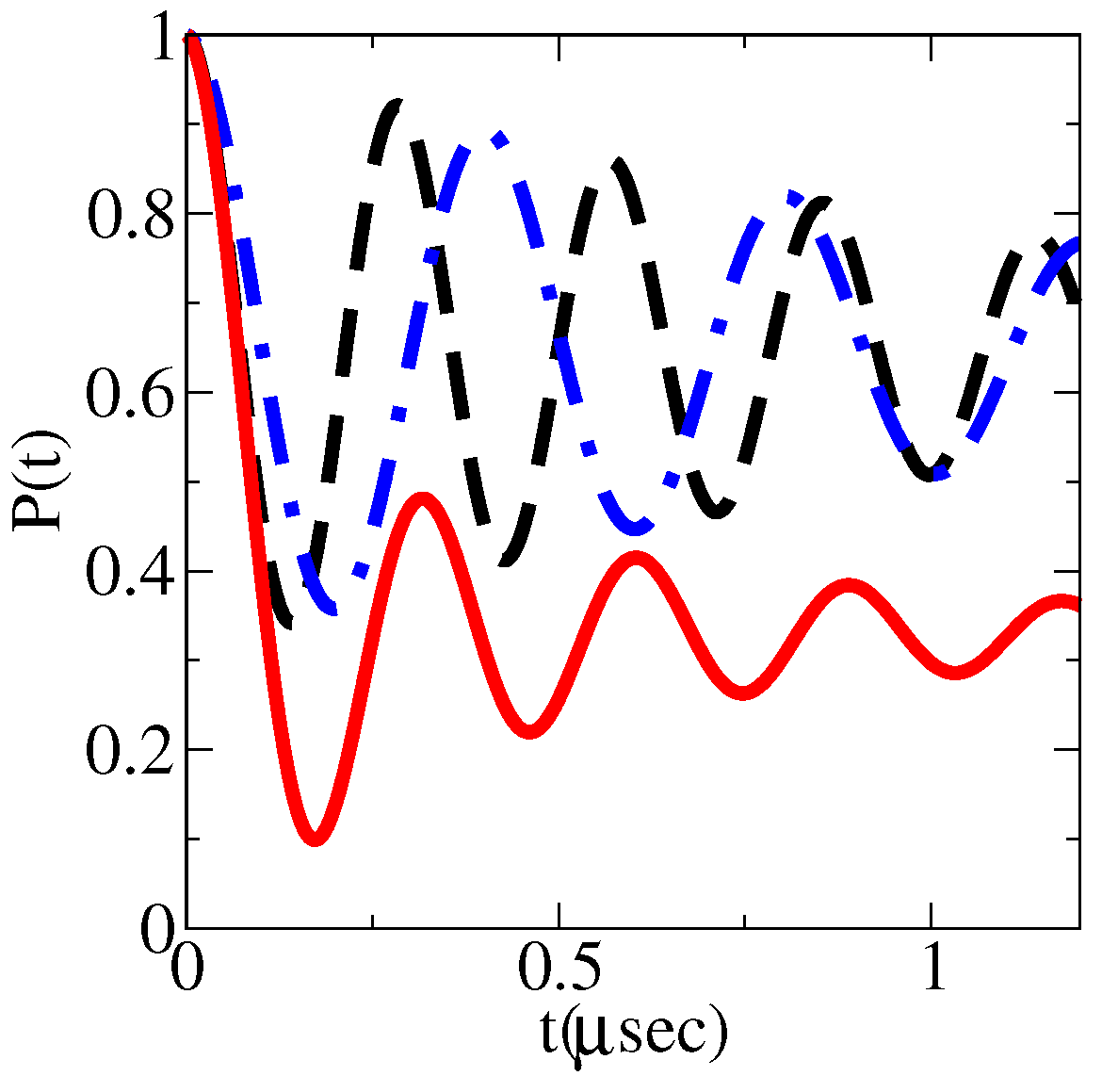
Consider now the case when the initial muon polarization is within the ${\mathrm{CuO}}_2$ plane. For the coplanar spin spiral averaging over directions of spins,

$$\begin{array}{c}\hfill \propto {\int }_0^{2\pi }cos(\omega tcos\alpha )d\alpha \propto J_0\left(\omega t\right),\end{array}$$

(13)

gives exactly Equation (5). The corresponding depolarization curve identical to that in Figure 2a is plotted in Figure 7 by the red solid line.

Figure 7. Depolarization plots for initial muon polarization in ${\mathrm{CuO}}_2$ plane. The solid red line corresponds to the spin spiral. The curve is independent of the orientation of the initial muon spin with respect to axes of the square lattice. The black dashed line and the blue dashed–dotted line correspond to the collinear spin stripe model. For the black dashed line, the initial muon spin is directed along the CuO link of the square lattice. For the blue dashed–dotted line, the initial muon spin is directed along the diagonal of the square lattice.

In the collinear spin stripe state, electron spins are directed along CuO-links of the ${\mathrm{CuO}}_2$ plane. Therefore, if initial muon spin is directed along a CuO-link the sites with spins along this link do not contribute to the depolarization, and sites with spins orthogonal to this direction give the maximum possible depolarization rate. Therefore, the $\mu$SR signal is

$$\begin{array}{c}\hfill P\left(t\right)={\displaystyle \frac{1}{2}}{U}_m(e^{-{\lambda }_{T}t}cos\left(\omega t\right)+1)+(1-U_m)\end{array}$$

(14)

This depolarization curve shown by the black dashed line in Figure 7 is very distinct from the spin spiral depolarization curve.

Moreover, if the initial muon spin is directed along a diagonal of the ${\mathrm{CuO}}_2$ plane, the magnetic field makes a $45°$ angle with the spin. Hence, the $\mu$SR signal is

$$\begin{array}{c}\hfill P\left(t\right)={\displaystyle \frac{1}{2}}{U}_m(e^{-{\lambda }_{T}t}cos(\omega t/\sqrt{2})+1)+(1-U_m)\end{array}$$

(15)

This depolarization curve shown by the blue dashed–dotted line in Figure 7 is very different from the two previous curves. In the plots presented in Figure 7, I used parameters determined in the polycrystalline experiment. Of course, in the single crystal, the value $U_m$ can be somewhat different, but independent of $U_m$ the shapes of the depolarization curves and even the frequencies are dramatically different and this gives a way to distinguish the models.

9. Conclusions

The $\mu$SR data indicate a single (site-independent) depolarization magnetic field. This is generically consistent with the coplanar in-plane spiral structure of spins in ${\mathrm{La}}_{2-x}{\mathrm{Ba}}_x{\mathrm{CuO}}_4$ ($x={\displaystyle \frac{1}{8}}$) and generically inconsistent with the spin stripe structure. However, with fine tuning of parameters of the spin stripe, one can make the spin stripe model consistent with existing $\mu$SR data. A $\mu$SR tomography experiment is suggested to reject or accept the fine-tuning scenario.

References

- Tranquada, J.M.; Sternlieb, B.J.; Axe, J.D.; Nakamura, Y.; Uchida, S. Evidence for stripe correlations of spins and holes in copper oxide superconductors. Nature 1995, 375, 561–563. [Google Scholar] [CrossRef] [Scilit]
- Tranquada, J.M.; Axe, J.D.; Ichikawa, N.; Nakamura, Y.; Uchida, S.; Nachumi, B. Neutron-scattering study of stripe-phase order of holes and spins in La1.48Nd0.4Sr0.12CuO4. Phys. Rev. B 1996, 54, 7489. [Google Scholar] [CrossRef] [Scilit] [PubMed]
- Yamada, K.; Lee, C.H.; Kurahashi, K.; Wada, J.; Wakimoto, S.; Ueki, S.; Kimura, H.; Endoh, Y.; Hosoya, S.; Shirane, G.; et al. Doping dependence of the spatially modulated dynamical spin correlations and the superconducting-transition temperature in La2−xSrxCuO4. Phys. Rev. B 1998, 57, 6165. [Google Scholar] [CrossRef] [Scilit]
- Fujita, M.; Yamada, K.; Hiraka, H.; Gehring, P.M.; Lee, S.H.; Wakimoto, S.; Shirane, G. Static magnetic correlations near the insulating-superconducting phase boundary in La2−xSrxCuO4. Phys. Rev. B 2002, 65, 064505. [Google Scholar] [CrossRef] [Scilit]
- Hinkov, V.; Pailhes, S.; Bourges, P.; Sidis, Y.; Ivanov, A.; Kulakov, A.; Lin, C.T.; Chen, D.P.; Bernhard, C.; Keimer, B. Two-dimensional geometry of spin excitations in the high-transition-temperature superconductor YBa2Cu3O6+x. Nature 2004, 430, 650–654. [Google Scholar] [CrossRef] [Scilit] [PubMed][Green Version]
- Hinkov, V.; Haug, D.; Fauque, B.; Bourges, P.; Sidis, Y.; Ivanov, A.; Bernhard, C.; Lin, C.T.; Keimer, B. Electronic liquid crystal state in the high-temperature superconductor YBa2Cu3O6.45. Science 2008, 319, 597–600. [Google Scholar] [CrossRef] [Scilit] [PubMed]
- Guguchia, Z.; Khasanov, R.; Bendele, M.; Pomjakushina, E.; Conder, K.; Shengelaya, A.; Keller, H. Negative Oxygen Isotope Effect on the Static Spin Stripe Order in Superconducting La2−xBaxCuO4 (x = 1/8) Observed by Muon-Spin Rotation. Phys. Rev. Lett. 2014, 113, 057002. [Google Scholar] [CrossRef] [Scilit] [PubMed]
- Kapon, I.; Salman, Z.; Mangel, I.; Prokscha, T.; Gavish, N.; Keren, A. Phase transition in the cuprates from a magnetic-field-free stiffness meter viewpoint. Nat. Commun. 2019, 10, 2463. [Google Scholar] [CrossRef] [Scilit] [PubMed]
- Grafe, H.-J.; Curro, N.J.; Young, B.L.; Vyalikh, A.; Vavilova, J.; Gu, G.D.; Hücker, M.; Büchner, B. Charge order and low frequency spin dynamics in lanthanum cuprates revealed by Nuclear Magnetic Resonance. Eur. Phys. J. Spec. Top. 2010, 188, 89–101. [Google Scholar] [CrossRef] [Scilit]
- Sushkov, O.P.; Kotov, V.N. Superconducting spiral phase in the two-dimensional t–j model. Phys. Rev. B 2004, 70, 024503. [Google Scholar] [CrossRef] [Scilit][Green Version]
- Lorenzana, J.; Seibold, G. Metallic Mean-Field Stripes, Incommensurability, and ChemicalPotential in Cuprates. Phys. Rev. Lett. 2002, 89, 136401. [Google Scholar] [CrossRef] [Scilit] [PubMed]
- Scholle, R.; Bonetti, P.M.; Vilardi, D.; Metzner, W. Comprehensive mean-field analysis of magnetic and charge orders in the two-dimensional Hubbard model. Phys. Rev. B 2023, 108, 035139. [Google Scholar] [CrossRef] [Scilit]
- Pinkpank, M.; Amato, A.; Andreica, D.; Gygax, F.N.; Ott, H.R.; Schenck, A. The effect of oxygen reduction on the magnetic properties of REBa2Cu3O6+x. Phys. C Supercond. 1999, 317–318, 299–303. [Google Scholar] [CrossRef] [Scilit]
- Ramadhan, M.R.; Adiperdana, B.; Ramli, I.; Sari, D.P.; Putri, A.E.; Widyaiswari, U.; Rozak, H.; Zaharim, W.N.; Manaf, A.; Kurniawan, B.; et al. Estimation of the on-site Coulomb potential and covalent state in La2CuO4 by muon spin rotation and density functional theory calculations. Phys. Rev. Res. 2022, 4, 033044. [Google Scholar] [CrossRef] [Scilit]
- Blundell, S.J.; Renzi, R.D.; Lancaster, T.; Pratt, F.L. (Eds.) Muon Spectroscopy—An Introduction; Oxford University Press: Oxford, UK, 2022. [Google Scholar]
- Budnick, J.I.; Golnik, A.; Niedermaye, C.; Recknagel, E.; Rossmanith, M.; Weidinger, A.; Chamberland, B.; Filipkowski, M.; Yang, D.P. Observation of magnetic ordering in La2CuO4 by muon spin rotation spectroscopy. Phys. Lett. A 1987, 124, 103–106. [Google Scholar] [CrossRef] [Scilit]
- Yamada, K.; Kudo, E.; Endoh, Y.; Hidaka, Y.; Oda, M.; Suzuki, M.; Murakami, T. The effect of the heat treatments on the antiferromagnetism in La2CuO4-δ single crystals. Solid State Commun. 1987, 64, 753–756. [Google Scholar] [CrossRef] [Scilit]
Disclaimer/Publisher’s Note: The statements, opinions and data contained in all publications are solely those of the individual author(s) and contributor(s) and not of MDPI and/or the editor(s). MDPI and/or the editor(s) disclaim responsibility for any injury to people or property resulting from any ideas, methods, instructions or products referred to in the content. |
© 2026 by the author. Licensee MDPI, Basel, Switzerland. This article is an open access article distributed under the terms and conditions of the Creative Commons Attribution (CC BY) license.