Bathymetric Structure and Recurrent Recruitment Hotspots of Juvenile Galeus melastomus Rafinesque, 1810 in the Central–Southern Tyrrhenian Sea

Abstract

Recruitment and the spatial distribution of early life stages govern the resilience of exploited elasmobranch populations, yet remain poorly understood in demersal sharks. We examined the bathymetric structure and recruitment hotspot recurrence of juvenile Galeus melastomus, a frequent by-catch of deep-water bottom trawling, in the central–southern Tyrrhenian Sea (GSA 10), using MEDITS data (2017–2024). Juveniles were defined as immature individuals (maturity stages 1–2) smaller than the sex-specific length at first maturity (L50: 384.1 mm in males, 425.1 mm in females). The Recruit Density Index (RDI, juveniles/km²) was compared among depth strata, analysed with a Tweedie generalised additive mixed model accounting for station and sampling season, and mapped by Inverse Distance Weighting; hotspot persistence was tested against random expectation. Juveniles occurred in every survey year, supporting continuous recruitment. Juvenile density was highest in the 201–500 m stratum (p < 0.001), peaking near 400 m. Densities were higher in autumn–winter surveys, and the model indicated a possible decline of about 12% per year requiring confirmation. Recruitment hotspots occurred mainly in this stratum and recurred at a small number of stations more often than expected by chance. These results can inform the monitoring and management of demersal elasmobranch by-catch in the Mediterranean Sea.

1. Introduction

Recruitment is one of the fundamental demographic processes governing the dynamics and resilience of marine populations, particularly in species with slow life histories such as elasmobranchs [1,2]. These traits—late maturity, low fecundity and long generation times—make sharks and rays exceptionally vulnerable to fishing mortality, and overfishing has now driven more than one-third of all chondrichthyans towards a high risk of extinction worldwide [3]. The Mediterranean Sea is among the regions of greatest concern, hosting one of the highest proportions of threatened cartilaginous fishes in the world as a consequence of its long and intense history of exploitation [4,5]. In this context, understanding where and when the early life stages of demersal sharks concentrate is a prerequisite for any spatially explicit management strategy. This is explicitly recognised in the regulatory framework currently in force: Regulation (EU) 2019/1241 establishes technical measures for the protection of marine ecosystems, including provisions on elasmobranch by-catch [6]; GFCM Recommendation GFCM/44/2021/16 introduced additional mitigation measures for the conservation of Mediterranean elasmobranchs [7]; and the GFCM 2030 Strategy identifies the protection of essential fish habitats as an operational priority [8]. Recent reviews nonetheless report persistent gaps and inconsistencies in how these instruments are implemented across the basin, and call for a more precautionary and spatially informed approach [9,10].

The spatial distribution of early life stages plays a crucial role in regulating juvenile survival by influencing growth and mortality and, consequently, the number of individuals that reach maturity and contribute to the adult population [11]. In many marine taxa, juveniles show marked spatial segregation from adults, commonly interpreted as the outcome of habitat-selection processes associated with food availability, reduced predation risk and favourable environmental conditions [12,13]. For elasmobranchs, the nursery concept was formalised by Heupel et al. [13], who proposed three criteria for identifying a nursery area: a higher density of juveniles than that observed in other areas, prolonged residence or use of the area by immature individuals, and recurrent use of the area over time. Subsequent studies have refined this framework, emphasising that nursery function should be assessed quantitatively rather than assumed [14]. Many species do not exhibit stable, permanent nurseries, but instead use dynamic recruitment habitats whose distribution varies among years in response to environmental conditions and anthropogenic pressures [15]. Determining whether juvenile aggregations meet the classical nursery criteria or instead represent temporary habitats is therefore central to both the spatial ecology of the species and the design of effective management measures [16,17].

Galeus melastomus Rafinesque, 1810, commonly known as the blackmouth catshark, is a demersal shark widely distributed throughout the Mediterranean Sea, except in the central and northern Adriatic Sea [18]. The species mainly inhabits soft-bottom habitats in epi- and mesobathyal environments and, across the Mediterranean, shows a tendency towards bathymetric segregation among age classes [19,20,21]. More recent analyses based on MEDITS data across the northern Mediterranean, and dedicated slope surveys, have confirmed this depth-related structuring and identified the species as one of the most abundant chondrichthyans on the Mediterranean slope [22,23]. Studies on its reproductive biology have suggested a continuous reproductive cyclicity in several Mediterranean areas, based on seasonal observations of gonadal maturity stages [20,24]; this hypothesis was subsequently confirmed in the study area [25]. Rey et al. [20] also reported that recruits and juveniles occur throughout the year with no evident seasonal patterns in abundance, and that mature individuals are consistently recorded, suggesting continuous reproduction. Across its range, G. melastomus is currently classified as Least Concern (LC) by the IUCN and occupies a broad bathymetric range (55 to 2000 m), although it is most commonly found between 200 and 500 m [26].

Although G. melastomus is not targeted by commercial fisheries, it represents a relevant component of the by-catch in deep-water bottom-trawl and longline fisheries [27,28,29,30]. Over the last decade, bottom trawlers have accounted for approximately 75% of the elasmobranch catches reported by EU fleets operating in the Mediterranean, of which around 40% were discarded [31]. Fishing pressure may therefore influence the spatial structure and dynamics of recruitment, making it necessary to understand the location and temporal stability of areas with the highest juvenile concentrations. Such knowledge is becoming increasingly relevant in a rapidly changing ocean, where warming, deoxygenation and increasing environmental variability are expected to interact with fishing pressure to reshape the distribution of demersal stocks, and where spatially and temporally adaptive management tools are needed to support elasmobranch populations caught as by-catch [32]. Although depth-related segregation, reproductive biology and juvenile occurrence of G. melastomus have been described in several Mediterranean areas [19,20,21,22,23,24,25], and nursery grounds have been identified in the adjacent GSA 9 [18], to our knowledge no multi-year assessment of juvenile density and of the location and temporal persistence of recruitment hotspots is available for the central–southern Tyrrhenian Sea (Geographical Sub-Area 10, GSA 10). Addressing this gap is the main novelty of the present study.

The general aim of this study was to characterise the juvenile component of G. melastomus in GSA 10 and its distribution in space and time, in order to identify where and when juveniles concentrate. The specific objectives were to: (1) estimate the sex-specific length at first maturity (L50) and use it, together with maturity stage, to identify juveniles; (2) quantify juvenile density and its variation among depth strata and years, taking into account sampling season and the repeated sampling of the same stations; (3) describe the spatial distribution of juvenile density and identify recruitment hotspots; and (4) assess the temporal persistence of these hotspots. Within this framework, two hypotheses were tested: (i) juvenile density was expected to be higher in the intermediate bathymetric stratum (201–500 m) than in the adjacent shallower and deeper strata, consistent with ontogenetic habitat segregation; and (ii) recruitment hotspots were expected to show low temporal persistence, with recurrence at the same stations not exceeding that expected by chance, which would indicate dynamic habitat use rather than stable nursery areas; conversely, recurrence at a small number of stations more often than expected by chance would indicate repeated use of the same sites.

2. Materials and Methods

2.1. Study Area and Data Collection

The data analysed were obtained from MEDITS (MEDiterranean International Trawl Survey) experimental bottom-trawl surveys carried out from 2017 to 2024 in GSA 10 (GFCM Geographical Sub-Area 10, central–southern Tyrrhenian Sea) [33,34]. MEDITS surveys are generally conducted between late spring and summer at depths ranging from 10 to 800 m. However, in several years of the time series (2017, 2020, 2021 and 2023), sampling was conducted later in the year, during autumn or winter. No survey was conducted in 2022, which was therefore excluded from the time series. Despite this seasonal heterogeneity, the same sampling design was applied in all years, with hauls distributed across five bathymetric strata (10–50, 51–100, 101–200, 201–500 and 501–800 m) according to a stratified random sampling design [34].

Hauls repeated at approximately the same location in different years were grouped into stations, which were used in the analysis of hotspot persistence (Section 2.3) and in the mixed model (Section 2.4). Haul duration was 30 min at depths down to 200 m and 60 min at greater depths, according to the MEDITS protocol [34]. Because haul codes were not consistent among years, stations were defined by agglomerative clustering of haul positions (projected in UTM zone 33N, WGS84), starting from the closest pairs of hauls carried out in different years. Two groups of hauls were merged only if all their hauls were less than 6 km apart (complete linkage), so that the maximum distance between any two hauls assigned to the same station was less than 6 km, and only if no year was represented more than once, so that each station included at most one haul per year. The 6 km threshold corresponds approximately to the length of a 60 min haul at about 3 knots. This procedure identified 78 stations. This threshold was preferred because the positions of hauls repeated at the same station varied more for the deeper 60 min hauls, where juveniles were concentrated: for these hauls, the nearest haul of another year lay within 6 km in 87% of cases, but within 3 km in only 75%. With a 6 km threshold, 29 of the 78 stations were sampled in all seven years, compared with 19 of 103 stations with a 3 km threshold.

For each individual collected during each survey year, total length (TL, mm), sex and maturity stage were recorded according to the MEDITS protocol.

Specimens were considered adults when classified as stage 3a (mature), 3b (mature/actively extruding), 4a (resting) and 4b (regenerating), and as immature when classified as stages 1 (immature–virgin) and 2 (maturing) [34].

2.2. Identification of Juveniles and Recruit Density Index

Length at first maturity (L50) was estimated separately for males and females using a logistic (ogive) model. The model was logit(P) = a + b · TL, where P is the probability of being mature and TL is total length, and L50 was calculated as −a/b. Confidence intervals at 95% (95% CI) were estimated by profile likelihood for parameters a and b, and by non-parametric bootstrap (5000 resamples, BCa method) for L50. Differences between sexes were tested with a likelihood-ratio test comparing a model with a single ogive for both sexes with a model with sex-specific intercept and slope, and by the bootstrap confidence interval of the difference between L50 values. The difference in slope was tested separately, by comparing the sex-specific model with a model with sex-specific intercepts and a common slope. The maturation range was expressed as the lengths at which 25% and 75% of individuals were mature (L25–L75), and model fit as the percentage of deviance explained. Individuals of indeterminate sex were excluded from the estimation of the ogives. Model fitting was performed in R version 4.5.1 [35]. Individuals shorter than the corresponding sex-specific L50 and classified as immature (stages 1 and 2) were considered juveniles, as were individuals of indeterminate sex, all of which were well below both L50 values. The maturity status of each individual was therefore assigned from its macroscopic maturity stage: L50, a population-level parameter, was not used as an individual maturity threshold but as an upper size limit within the immature fraction, in order to isolate the recruit component by excluding large immature individuals approaching maturity. Two checks were carried out to assess whether this exclusion was justified. First, the depth distribution of immature individuals with TL equal to or greater than the L50 was compared with that of juveniles and with that of mature individuals (Mann–Whitney tests), to determine whether they occurred in the juvenile or in the adult depth range. Second, the comparisons of juvenile density among depth strata (Section 2.3) were repeated including these individuals among juveniles, to assess whether their exclusion affected the results.

This procedure made it possible to estimate a Recruit Density Index (RDI; number of juveniles per square kilometre, juveniles/km²) for each haul. The swept area (km²) of each haul was calculated according to the MEDITS protocol [34] as the product of the distance trawled, derived from the GPS positions recorded at the start and end of the haul, and the mean horizontal (wing) opening of the net measured during the haul; RDI was then expressed as the number of juveniles per km² of swept area. Annual mean RDI was calculated as the arithmetic mean of the RDI values of all hauls carried out in each year, including those without juveniles (RDI = 0).

2.3. Spatial Interpolation and Hotspot Analysis

The spatial patterns of RDI were explored using Inverse Distance Weighting (IDW) interpolation implemented in QGIS version 3.34 “Prizren” [36]. IDW was used as an exploratory tool to visualise areas with the highest concentrations of juveniles; this method is particularly suitable for phenomena that vary continuously in space but are sampled at a limited number of locations, as it assigns greater weight to nearby points and progressively reduces the influence of more distant ones. A power parameter (P) of 2 was used, as commonly adopted in ecological studies, to ensure a quadratic decrease in the influence of sampling points with increasing distance. No limit was imposed on the number of neighbours, and all available points were therefore used to estimate the value of each cell. Since the analysis was not intended for formal geostatistical inference, IDW interpolation was considered appropriate given the spatial distribution and the available sampling density; more complex methods, such as kriging, were not adopted because a robust estimate of the experimental variogram was not available. IDW was applied to all hauls, including those without juveniles (RDI = 0), and was used for visualisation only. Because interpolation without a limit on the number of neighbours tends to smooth local maxima, the ability of IDW to reproduce the observed values was assessed by leave-one-out cross-validation within each year, comparing interpolation based on all points with interpolation based on the 4, 8 and 12 nearest neighbours. Agreement between predicted and observed values was measured by the Pearson correlation coefficient and, at hotspot hauls, by the median ratio of predicted to observed RDI; cross-validation was carried out in R version 4.5.1 [35].

Differences in RDI among bathymetric strata over the entire study period (2017–2024) were tested with Welch’s t-test using all hauls, including those without juveniles (RDI = 0), in the strata where juveniles were recorded (101–200, 201–500 and 501–800 m); the 10–50 m (44 hauls) and 51–100 m (52 hauls) strata were excluded because no juveniles were caught in them, so that RDI was zero in all hauls and the test could not be computed. This test was selected because it allows the means of two groups to be compared when variances and sample sizes are unequal, providing greater robustness than the conventional Student’s t-test. p-values of the three pairwise comparisons were adjusted for multiple comparisons using the Holm method. Welch’s t-tests and the boxplots of RDI across bathymetric strata were computed in R version 4.5.1 [35].

For each year, hauls were ranked by decreasing RDI and the cumulative RDI was calculated as a percentage of the annual total. Density hotspots were defined as the hauls required to reach 50% of the total annual RDI, including the haul at which the threshold was exceeded. The hotspot set ${\mathrm{H}}_{\mathrm{y}}$ was defined as the minimal subset of hauls such that

$$\sum \left(\mathrm{i}\in {\mathrm{H}}_{\mathrm{y}}\right){\mathrm{R}\mathrm{D}\mathrm{I}}_{\mathrm{i}}\ge 0.5\times \sum \left(\mathrm{i}\in {\mathrm{Y}}_{\mathrm{y}}\right){\mathrm{R}\mathrm{D}\mathrm{I}}_{\mathrm{i}}$$

where ${\mathrm{Y}}_{\mathrm{y}}$ is the set of all hauls carried out in the year y. The 50% threshold was chosen for two reasons. First, in each year, the hotspots are the smallest set of hauls that together account for half of the total annual RDI, i.e., at least as much as all the remaining hauls combined. Second, it balances two opposite requirements: lower thresholds (e.g., 25%) select only one or two hauls per year, too few to assess whether hotspots recur at the same stations, whereas higher thresholds (e.g., 75–90%) progressively include hauls with moderate or low densities, so that hotspots would no longer differ from the hauls in which juveniles were merely present. With the 50% threshold, every hotspot haul had an RDI at least twice the median RDI of the hauls with juveniles in the same year. Because the threshold is calculated on the total of each year, this criterion identifies the hauls in which juveniles were concentrated in a given year, regardless of overall abundance, and makes it possible to assess whether hotspots recur at the same locations across years. Since the number of hauls varied among years (from 37 in 2020 to 71 in 2021), and the number of hotspots also depends on how juveniles are distributed among the hauls of each year, the number of hotspots per year was not compared across years, and the analysis was based on their location. Hotspots were therefore derived from haul-level RDI values, not from the IDW surface. Hotspot persistence was evaluated at the station level, using the stations defined in Section 2.1, as the number of years in which each station was identified as a hotspot. To provide an objective reference, the observed persistence was compared with that expected by chance using permutation tests (9999 permutations). In each permutation, the observed number of hotspots of each year was reallocated at random among the hauls carried out in that year within the depth range occupied by juveniles (170–683.5 m; null model A), or among the hauls of the same depth stratum, preserving the number of hotspots per stratum and year (null model B), so as to account for the bathymetric preference of juveniles. Two statistics were compared with their null distributions: the number of recurrences (cases in which a station was a hotspot in more than one year) and the mean pairwise Jaccard similarity between the hotspot sets of different years; one-sided p-values were computed as the proportion of permutations yielding values equal to or greater than those observed. Persistence was considered low, as stated in hypothesis (ii), if the observed statistics did not exceed those expected by chance (p ≥ 0.05); the null distributions therefore provided the reference against which the observed overlap was judged, instead of an arbitrary fixed value of the Jaccard index. Hotspot and persistence analyses were performed in R version 4.5.1 [35], and maps were produced in QGIS version 3.34 “Prizren” [36].

2.4. Station-Level Mixed Model

To account for station-level variability, repeated sampling of the same locations and differences in sampling season, juvenile counts per haul were also analysed with a generalised additive mixed model (GAMM) with a Tweedie distribution and log link, which accommodates the high proportion of zero catches and the strong right skewness of the data. The model was fitted to all hauls deeper than 100 m (n = 348), since no juveniles were caught at shallower depths, with the number of juveniles per haul as the response variable and the logarithm of the swept area as an offset. Fixed effects included a smooth function of depth (thin plate regression spline, k = 6), sampling season (spring–summer: 2018, 2019 and 2024; autumn–winter: 2017, 2020, 2021 and 2023) and year as a linear trend; year (as a factor) and station were included as random intercepts. Stations were defined as described in Section 2.1; 62 of the 78 stations fell within the modelled depth range.

Because each survey was carried out in a single season, season and year are partly confounded, and the season effect is estimated from the contrast between years sampled in different seasons. Pairwise comparisons between depth strata were obtained from a second model, in which the depth smooth was replaced by depth stratum (101–200, 201–500 and 501–800 m) as a factor, using Wald tests with Holm correction. The significance of parametric terms (season and linear trend) was assessed with t-tests, and that of the depth smooth and of the random effects with approximate F-tests [37]. The contribution of depth, sampling season, linear trend and station was assessed by refitting the model without each of these components in turn and calculating the increase in the Akaike Information Criterion (ΔAIC) relative to the full model (maximum likelihood fits); the larger the ΔAIC, the greater the contribution of the component. Model fit was checked with simulation-based randomised quantile residuals and by comparing the observed number of zero catches with the number expected from simulations of the fitted model.

A model-standardised annual index was obtained, for each year, by averaging model predictions over the depths of all modelled hauls (a common set of depths for all years), for an average station (i.e., setting station random effects to zero); each year retained its own sampling season. 95% confidence intervals were derived from 4000 draws of the model coefficients. Models were fitted with the mgcv package [37] in R version 4.5.1 [35].

3. Results

3.1. Length at First Maturity

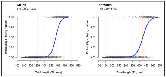
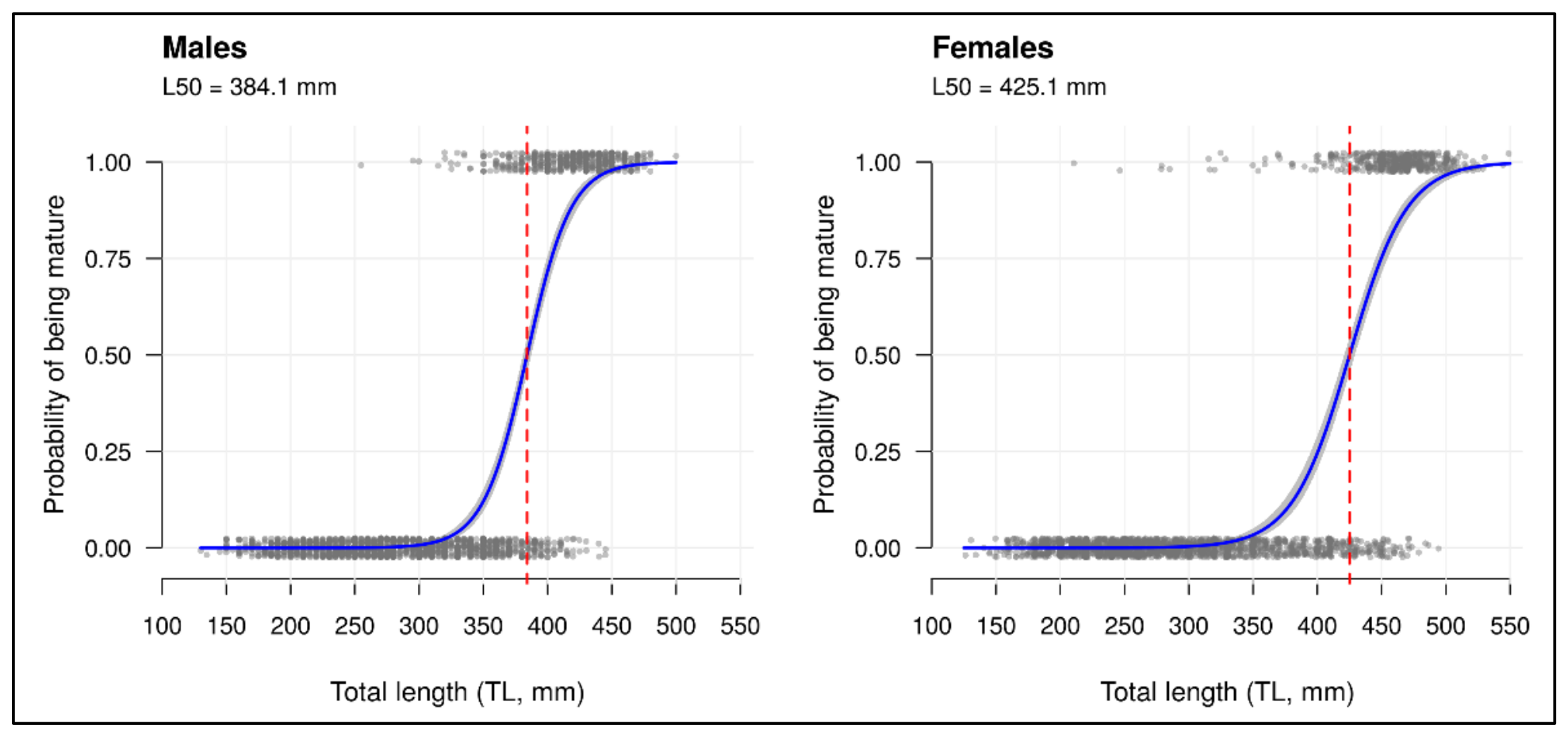
The relationship between total length (TL) and the probability of being mature was modelled separately for males and females using logistic regression (Figure 1). A total of 4365 individuals were analysed, including 2150 males, 2109 females and 106 individuals of indeterminate sex. Individuals of indeterminate sex were excluded from the estimation. A sigmoidal pattern, typical of maturation processes, was observed in both sexes. The estimated L50—corresponding to the length at which 50% of individuals are mature—was 384.1 mm (95% CI 381.0–387.3) for males and 425.1 mm (95% CI 420.8–428.9) for females (Table 1). Females reached maturity at significantly larger sizes than males (difference between L50 values: 41.1 mm; 95% CI 36.0–46.3 mm). The ogives differed significantly between sexes (likelihood-ratio test: χ² = 230.5, df = 2, p < 0.001), including in slope (χ² = 12.3, df = 1, p < 0.001), with a wider maturation range (L25–L75) in females (400.5–449.7 mm) than in males (365.2–402.9 mm). The distribution of the observed data and the relatively narrow confidence intervals around the curves indicate a good model fit (deviance explained: 69.9% in males and 66.9% in females) and reasonable precision in parameter estimation. Among immature individuals, 156 (3.7% of sexed individuals) had a TL equal to or greater than the L50 of their sex (80 males, TL 385–445 mm; 76 females, TL 430–495 mm), almost all at stage 2 (154 individuals); these individuals were not considered juveniles. Their depth distribution was similar to that of mature individuals (median depth 579 vs. 582 m; Mann–Whitney test, p = 0.52) and differed from that of juveniles (median depth 401 m; p < 0.001), with 74% of them caught in the 501–800 m stratum, compared with 31% of juveniles. Including them among juveniles would have increased the number of juveniles by 4.9% and the number of hauls with juveniles from 197 to 199, without changing the differences in RDI among depth strata (Welch’s t-tests, Holm-adjusted p ≤ 0.001). Conversely, 74 males and 56 females with TL below the L50 were mature.

Figure 1. Relationship between total length (TL, mm) and the probability of being mature in males (left) and females (right). Grey dots represent individual specimens (0 = immature; 1 = mature), slightly jittered to reduce overlap. The curves represent the fitted logistic regression models with 95% confidence intervals (shaded areas). The red dashed line indicates the length at which 50% of individuals are mature (L50). Individuals at stages 1 and 2 were considered immature.

Table 1. Maturity ogive parameters of G. melastomus in GSA 10 (2017–2024): sample size by sex, total length range, parameters of the logistic model logit(P) = a + b · TL with 95% CI (profile likelihood), L50 with 95% CI (BCa bootstrap), maturation range (L25–L75) and deviance explained.

Parameter	Males	Females
n (immature/mature)	2150 (1591/559)	2109 (1627/482)
TL min–max (mm)	130–500	125–550
a (95% CI)	−22.39 (−24.79, −20.22)	−19.00 (−21.20, −17.02)
b (95% CI)	0.0583 (0.0526, 0.0645)	0.0447 (0.0401, 0.0498)
L50, mm (95% CI)	384.1 (381.0–387.3)	425.1 (420.8–428.9)
L25–L75 (mm)	365.2–402.9	400.5–449.7
Deviance explained (%)	69.9	66.9

3.2. Abundance and Temporal Trend of Juveniles

Over the 2017–2024 period, a total of 4365 specimens of G. melastomus were caught, of which 3159 (including 106 individuals of indeterminate sex) were juveniles (72.37% of the total). Juveniles were recorded in 197 of the 444 hauls (44.37%), at depths ranging from 170 to 683.5 m. They were consistently recorded across all MEDITS surveys, regardless of the sampling season (Table 2).

Table 2. Total annual catches and number of juveniles of G. melastomus recorded during MEDITS surveys (2017–2024), with juveniles expressed as percentage of the total catch for each year.

Year	Total Individuals	Juveniles	Juveniles (%)
2017	1360	946	69.6
2018	738	520	70.5
2019	543	323	59.5
2020	256	200	78.1
2021	716	561	78.4
2023	380	317	83.4
2024	372	292	78.5

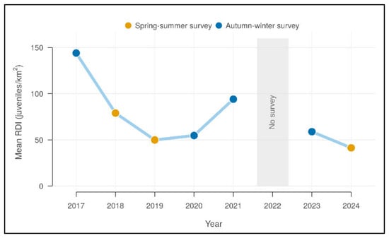
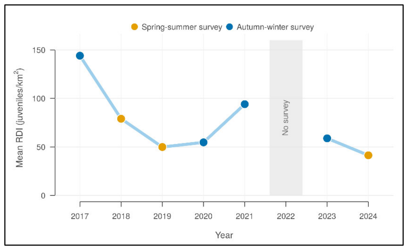
The annual mean of the RDI (Figure 2), calculated over all hauls, varied markedly among years, with the highest values in 2017 and 2021, both sampled in autumn–winter, and the lowest value in 2024. In both seasons, the most recent survey had a lower mean than the earliest one (autumn–winter: 144.0 juveniles/km² in 2017 vs. 58.9 juveniles/km² in 2023; spring–summer: 79.0 juveniles/km² in 2018 vs. 41.4 juveniles/km² in 2024). However, annual means do not separate the temporal trend from differences in sampling season and among stations, which were accounted for in the station-level model (Section 3.7).

Figure 2. Annual mean Recruit Density Index (RDI) values of G. melastomus from 2017 to 2024. The solid line connects the annual mean values of consecutive survey years and is interrupted in 2022, when no survey was carried out (grey band). Annual means were calculated over all hauls, including those without juveniles. Point colours indicate the sampling season (spring–summer: 2018, 2019 and 2024; autumn–winter: 2017, 2020, 2021 and 2023).

3.3. Spatial Distribution of Recruit Density

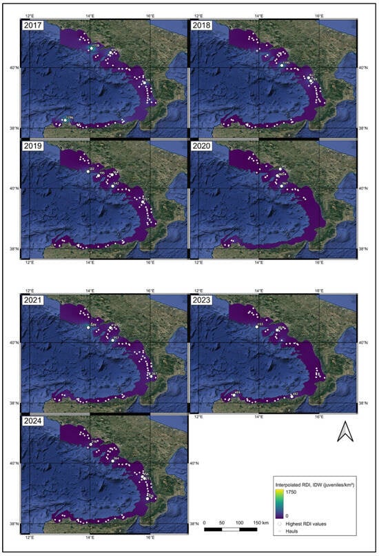
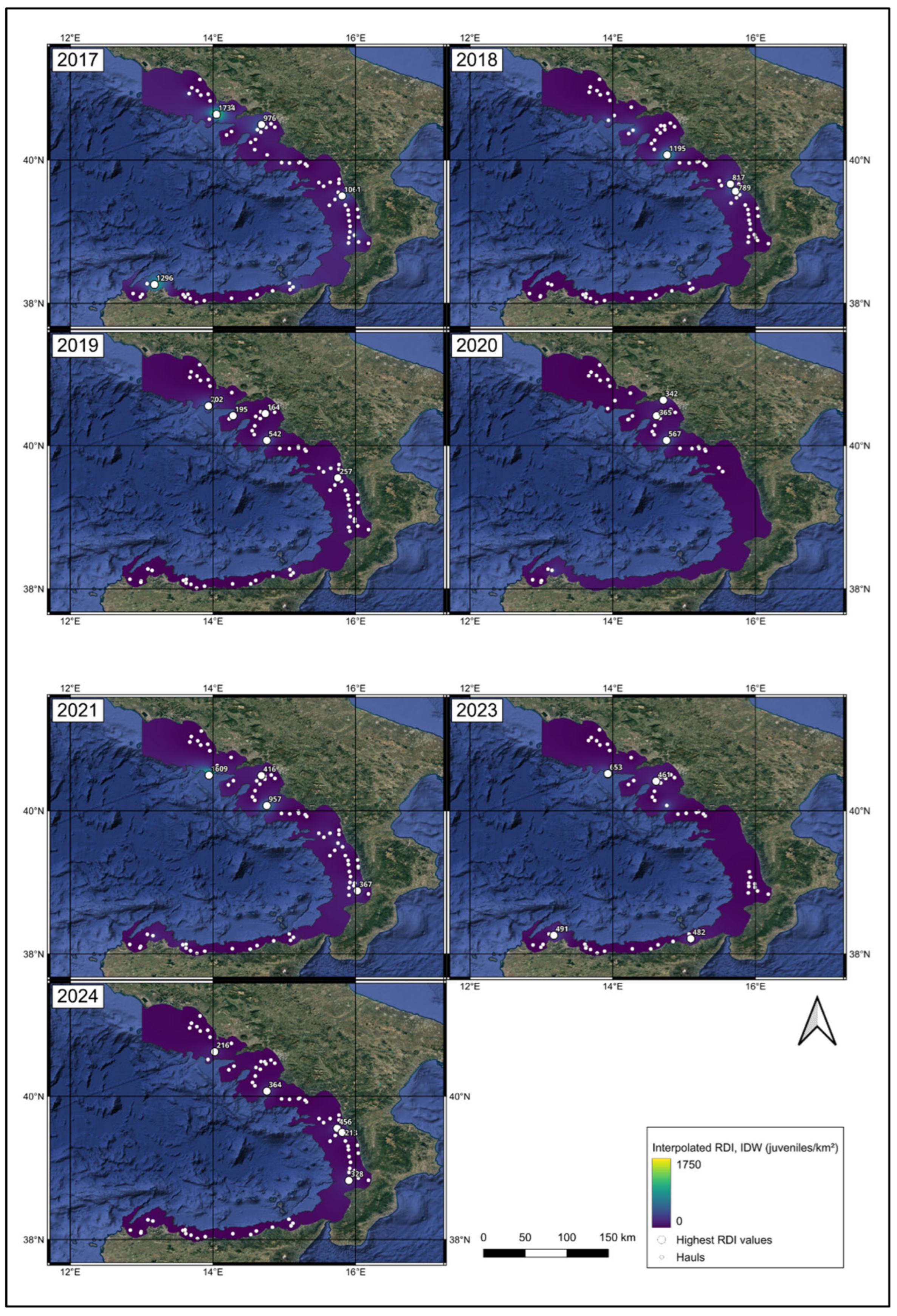
The spatial distribution of RDI from 2017 to 2024 (Figure 3) is shown on a colour scale common to all years (0–1750 juveniles/km²), from purple (low density) to yellow (high density). Haul-level RDI values ranged from 0 (247 hauls) to 1734 juveniles/km². The interpolated surfaces were dominated by low values, with localised peaks around the hauls with the highest RDI, whose position and intensity varied among years. Leave-one-out cross-validation showed that IDW predictions at unsampled hauls were poorly correlated with the observed RDI (r = 0.11 using all points; r = 0.09 using the 4–12 nearest neighbours) and underestimated RDI at hotspot hauls by about 90%, irrespective of the number of neighbours, confirming that the interpolated surfaces smooth local maxima and are suitable for visualisation only.

Figure 3. Spatial distribution of the Recruit Density Index (RDI) of G. melastomus for each year from 2017 to 2024. Values were interpolated by Inverse Distance Weighting (power = 2) from all hauls, including those without juveniles, and are shown on a colour scale common to all years (0–1750 juveniles/km²), from lower (purple) to higher (yellow) values. Small white points indicate the hauls; larger white circles indicate the hotspot hauls (Section 3.5), labelled with their RDI value (juveniles/km²).

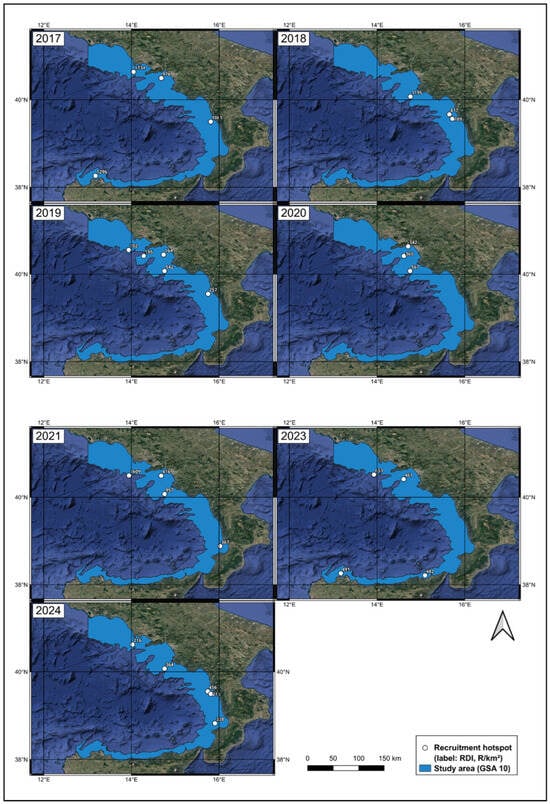
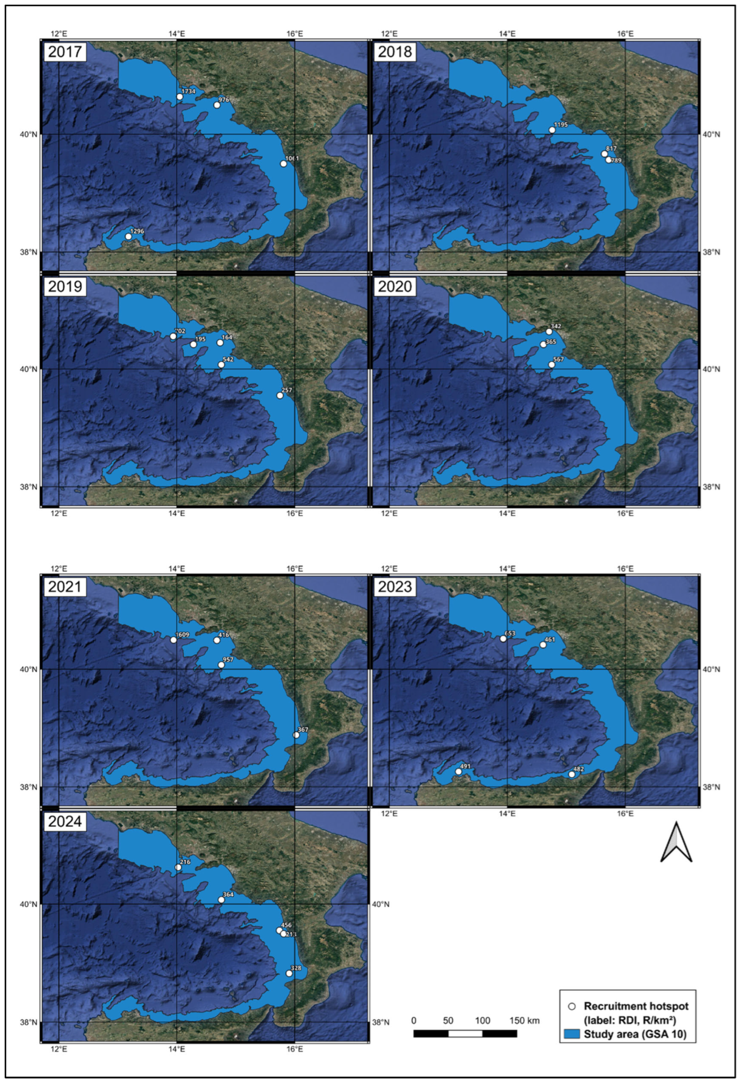
The highest values were recorded in 2017 (up to 1734 juveniles/km² in the Gulf of Naples, and between 976 and 1296 juveniles/km² off Punta Raisi, off the northern Calabrian coast and in the Gulf of Salerno) and in 2021 (1609 juveniles/km² off Ischia and 957 juveniles/km² off Castellabate), followed by 2018 (1195 juveniles/km² off Castellabate). In the remaining years, the maximum values were lower, ranging from 456 juveniles/km² in 2024 to 702 juveniles/km² in 2019.

In all years, the highest values occurred mainly at intermediate depths, and their location changed among years, although high values recurred at some stations, such as off Castellabate (Section 3.5 and Section 3.6). The detailed annual variation is summarised in Table 3.

Table 3. Annual variation of the Recruit Density Index (RDI, juveniles/km²) of G. melastomus in GSA 10 (2017–2024), including mean ± standard deviation (SD), maximum RDI, number of recruitment hotspots and predominant bathymetric stratum. Mean, SD and maximum were calculated over all hauls, including those without juveniles; the predominant stratum refers to hotspots.

Year	Mean RDI ± SD (Juveniles/km2)	Max RDI (Juveniles/km2)	Recruitment Hotspots (n)	Predominant Bathymetric Stratum (m)
2017	143.98 ± 322.77	1734	4	201–500
2018	79.02 ± 209.86	1195	3	201–500
2019	49.92 ± 114.96	702	5	201–500/501–800
2020	54.73 ± 128.60	567	3	201–500
2021	94.05 ± 233.10	1609	4	201–500
2023	58.86 ± 147.90	653	4	201–500
2024	41.40 ± 88.66	456	5	201–500

3.4. Bathymetric Segregation

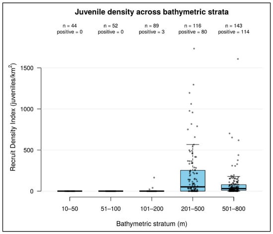
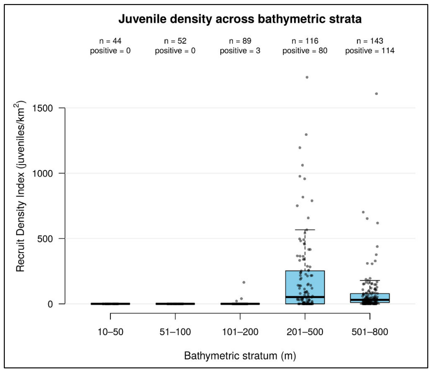
Considering all hauls, including those without juveniles, mean RDI was 2.5 juveniles/km² in the 101–200 m stratum (3 positive hauls out of 89), 194.0 juveniles/km² in the 201–500 m stratum (80 of 116) and 78.8 juveniles/km² in the 501–800 m stratum (114 of 143), whereas no juveniles were recorded in the 10–50 and 51–100 m strata (44 and 52 hauls, respectively). Welch’s t-test revealed significant differences between all pairs of strata: 101–200 vs. 201–500 m (t = −6.68, df = 116.0, p < 0.001), 101–200 vs. 501–800 m (t = −5.25, df = 147.0, p < 0.001) and 201–500 vs. 501–800 m (t = 3.60, df = 171.8, p < 0.001). All comparisons remained significant after Holm correction (p < 0.001). These results indicate that the intermediate stratum was clearly characterised by higher recruitment densities, consistent with the boxplot shown in Figure 4.

Figure 4. Distribution of the Recruit Density Index (RDI, juveniles/km²) across bathymetric strata, calculated over all hauls (including those without juveniles, RDI = 0). Points represent individual hauls; the number of hauls (n) and of hauls with juveniles (positive) is shown for each stratum.

The 201–500 m stratum showed the highest median RDI (51.7 juveniles/km²) and the greatest dispersion, with values up to 1734 juveniles/km². The 501–800 m stratum had a lower median (31.0 juveniles/km²) but the highest proportion of positive hauls (79.7%) and some high values (up to 1609 juveniles/km²), suggesting the occasional occurrence of high juvenile concentrations at greater depths. In the 101–200 m stratum, juveniles were recorded in only 3 of 89 hauls (3.4%), all at depths of 170 m or more, so the boxplot is flattened at zero; in the 10–50 and 51–100 m strata RDI was always zero.

3.5. Recruitment Hotspots

The spatial analysis of recruitment hotspots showed marked spatial and temporal variability in their distribution (Figure 5).

Figure 5. Spatial location of the recruitment hotspots identified from 2017 to 2024. For each year, the maps show the hauls identified as hotspots, i.e., the hauls with the highest RDI that together accounted for 50% of the annual total. White circles indicate the hotspot hauls, each labelled with its RDI value (juveniles/km²); the light blue area indicates the study area (GSA 10). Background: Google Satellite imagery (© Google), in which dark blue tones represent the sea and green–brown tones represent land.

The number of hotspots identified each year is reported in Table 3; because it depends on the number of hauls carried out and on the concentration of juveniles within each year, it was not compared across years.

Areas characterised by the highest RDI values varied among years and occurred in the northern (Gulf of Naples and Gulf of Salerno), central (Castellabate), eastern (off the northern Calabrian coast and in the Gulf of Sant’Eufemia) and southern (Punta Raisi, Gulf of Patti) sectors of the basin, with some stations recurring in more than one year (Section 3.6). The maximum RDI among hotspots ranged from 456 juveniles/km² (2024) to 1734 juveniles/km² (2017), with no progressive decline over time.

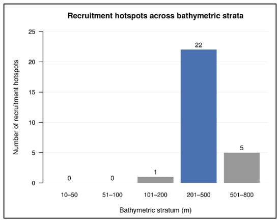
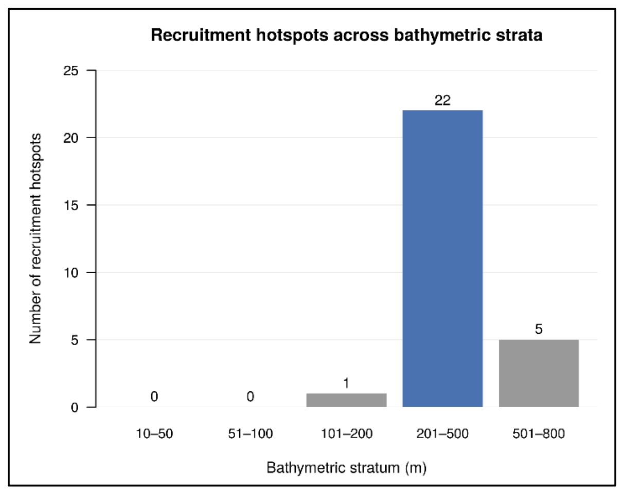
The distribution of hotspots across depth strata (Figure 6) showed a clear bathymetric preference for the 201–500 m stratum, with 22 hotspots located within this depth range, compared with 5 in the deeper stratum (501–800 m) and 1 in the 101–200 m stratum. This pattern is consistent with the RDI distribution maps, in which sampling stations with the highest values tended to occur within the same depth range.

Figure 6. Number of recruitment hotspots identified across depth strata, pooled over the seven survey years (2017–2024; n = 28 hotspot hauls). Numbers above the bars indicate the number of hotspots; the 201–500 m stratum, which included most hotspots, is highlighted in blue. No juveniles were caught in the 10–50 and 51–100 m strata.

3.6. Temporal Persistence of Hotspots

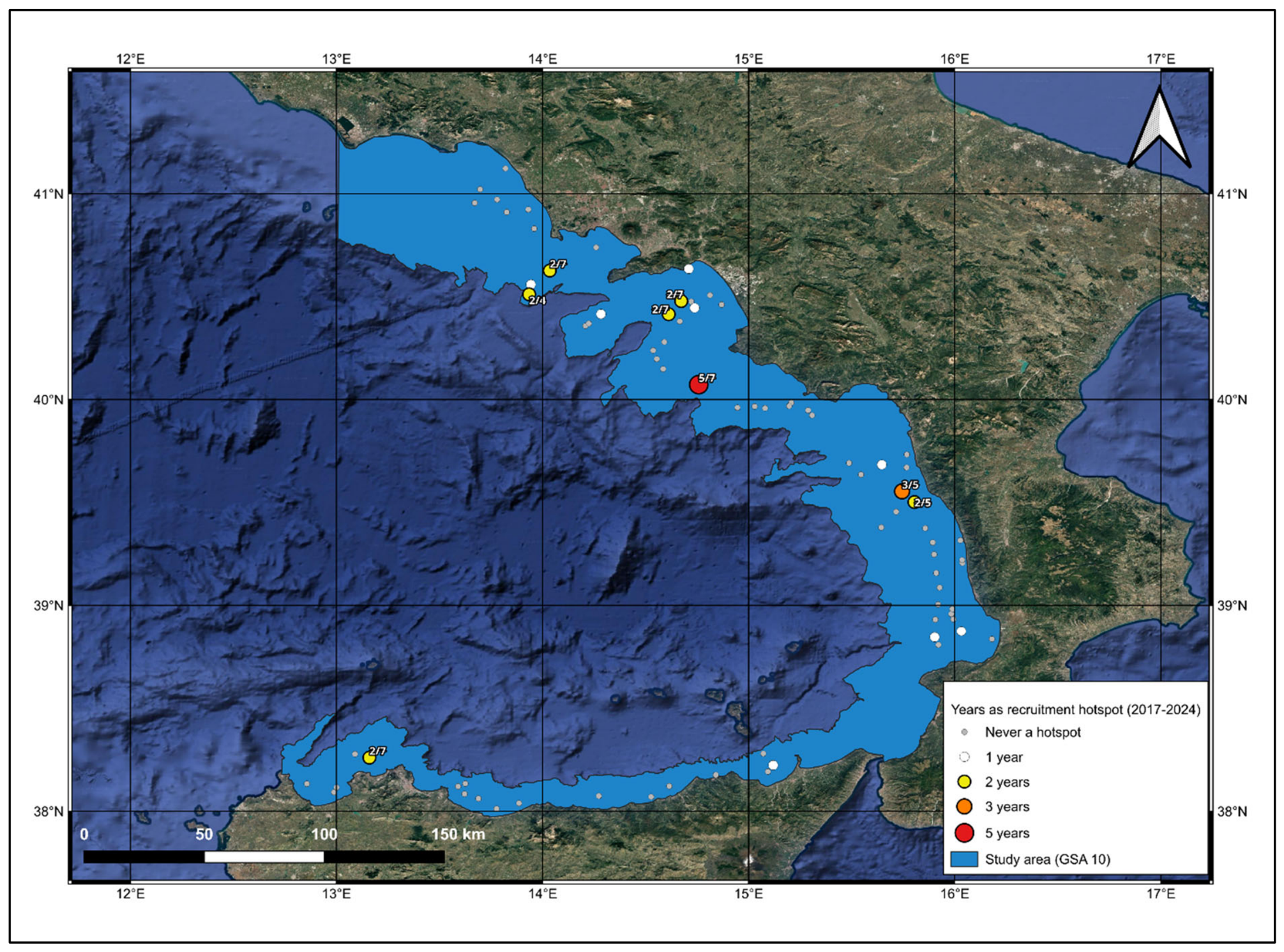
Over the seven survey years, the 28 hotspot hauls corresponded to 16 stations (Figure 7): eight stations were hotspots in a single year, six in two years, one off the northern Calabrian coast in three years (2018, 2019 and 2024) and one, located off Castellabate at about 365 m depth, in five of the seven years (2018–2021 and 2024). Stations identified as hotspots in two years were located in the Gulf of Naples (two stations, one of them off Ischia), in the Gulf of Salerno (two stations), off the northern Calabrian coast and off Punta Raisi. Hotspot recurrence was higher than expected by chance: the 12 recurrences observed (cases in which a station was a hotspot in more than one year) exceeded those expected when hotspots were randomly reallocated among hauls within the depth range occupied by juveniles (null model A: mean 6.0, 95% range 3–9; p < 0.001) and when they were reallocated within depth strata (null model B: mean 8.4, 95% range 6–11; p = 0.023). Similarly, the mean pairwise Jaccard similarity between the hotspot sets of different years (0.14) was higher than expected under both null models (0.047, p < 0.001; and 0.079, p = 0.018).

Figure 7. Temporal persistence of recruitment hotspots at the sampling stations over the 2017–2024 period. Symbol size and colour indicate the number of years in which each station was identified as a hotspot (white, 1 year; yellow, 2 years; orange, 3 years; red, 5 years); for recurrent stations, labels report the number of hotspot years over the number of years sampled. Grey dots indicate stations never identified as hotspots. The light blue area indicates the study area (GSA 10). Background: Google Satellite imagery (© Google), in which dark blue tones represent the sea and green–brown tones represent land.

3.7. Effects of Depth, Season and Year on Juvenile Density

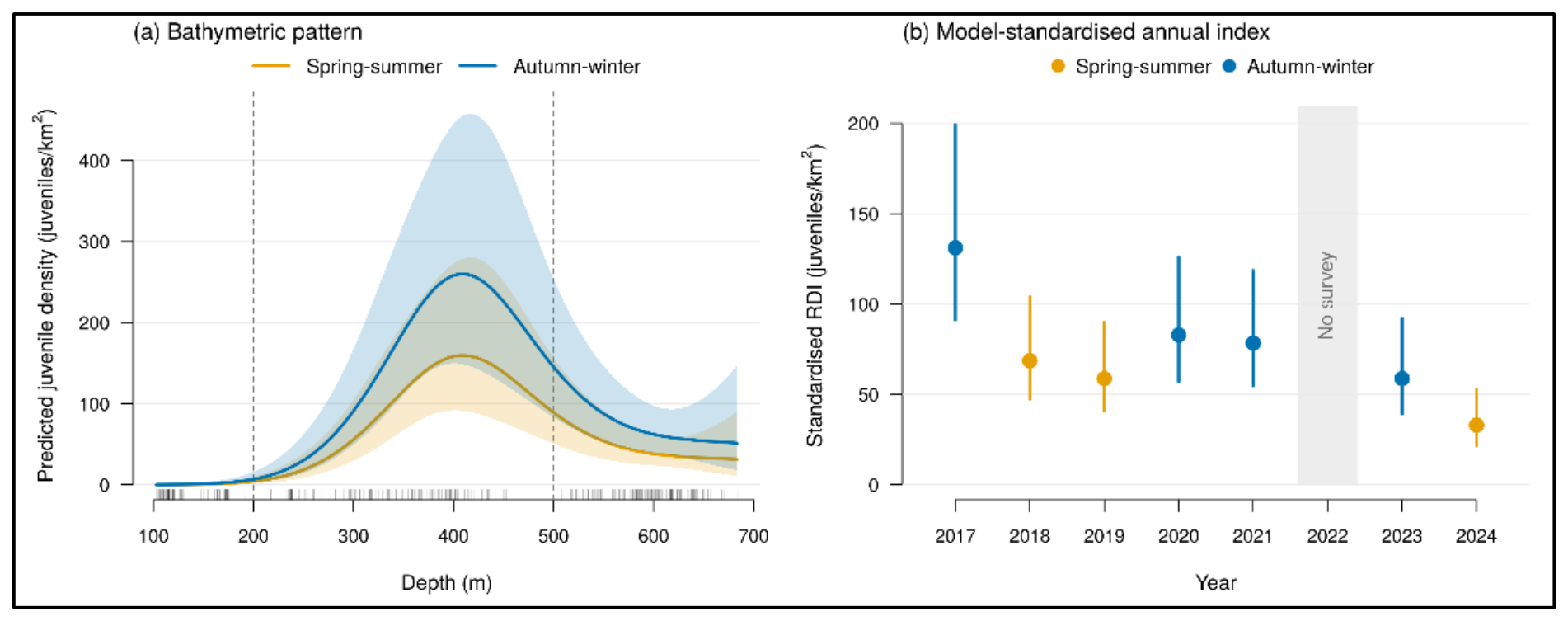
The Tweedie GAMM explained 60.9% of the deviance, and simulation-based residuals showed no marked departure from the assumed distribution (160 zero catches predicted vs. 151 observed). Station was the most important random component (ΔAIC = 60.1 when removed), indicating consistent differences in juvenile density among locations across years (Table 4). Depth had a strong non-linear effect (ΔAIC = 33.5), with predicted density peaking at around 400 m and declining at greater depths (Figure 8a). Densities in the 201–500 m stratum were 2.0 times higher than in the 501–800 m stratum (95% CI 1.02–4.03; p = 0.044) and about 70 times higher than in the 101–200 m stratum (p < 0.001). Autumn–winter surveys yielded densities 1.6 times higher than spring–summer surveys (95% CI 1.2–2.2; p = 0.003). After accounting for depth, season and station, the model indicated a possible decline in juvenile density of about 12% per year (density ratio 0.88 per year; 95% CI 0.83–0.94; p < 0.001), and the model-standardised annual index was 131 juveniles/km² in 2017 and 33 juveniles/km² in 2024 (Figure 8b). However, the reduction in AIC provided by the season and trend terms was modest (ΔAIC = 1.5 and 1.3, respectively), and the residual year-to-year variation was negligible once these terms were included. Given this modest support, the partial confounding between season and year and the short time series, the decline should be regarded as possible and requiring confirmation.

Table 4. Results of the Tweedie generalised additive mixed model (GAMM) of juvenile counts per haul of G. melastomus (n = 348 hauls deeper than 100 m; 62 stations), with log swept area as offset. Season, trend and stratum effects are expressed as density ratios with 95% confidence intervals; stratum contrasts were obtained from the model with depth stratum as a factor (Wald tests, Holm-adjusted p-values). edf: effective degrees of freedom. Test statistics: t, t-test for parametric terms (season and linear trend); F, approximate F-test for the depth smooth and the random effects; z, Wald test for the contrasts between depth strata.

Term	Estimate (95% CI)	Test Statistic	p
Depth (smooth)	edf = 3.87	F = 20.38	<0.001
Season (autumn–winter vs. spring–summer)	1.63 (1.19–2.24)	t = 3.03	0.003
Year (linear trend, per year)	0.88 (0.83–0.94)	t = −3.74	<0.001
Year (random effect)	edf = 0.72	F = 0.21	0.334
Station (random effect)	edf = 33.13	F = 1.76	<0.001
201–500 vs. 501–800 m	2.03 (1.02–4.03)	z = 2.01	0.044
201–500 vs. 101–200 m	73.5 (23.9–225.9)	z = 7.51	<0.001
501–800 vs. 101–200 m	36.3 (11.7–112.6)	z = 6.22	<0.001

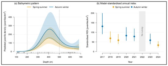
Figure 8. Results of the Tweedie GAMM of juvenile counts per haul. (a) Predicted juvenile density (juveniles/km²) as a function of depth for spring–summer and autumn–winter surveys (year at its mean value, station effects excluded), with 95% confidence bands; dashed lines mark the 200 and 500 m stratum boundaries, and ticks on the x-axis show the depths of the sampled hauls. (b) Model-standardised annual index of juvenile density with 95% confidence intervals, coloured by sampling season. No survey was carried out in 2022 (grey band).

4. Discussion

The present study provides an integrated assessment of the abundance dynamics and spatio-temporal distribution of juvenile G. melastomus in GSA 10, contributing to expanding current knowledge of the juvenile component of the species in the central–southern Tyrrhenian Sea. The integration of morphometric data, density indices and spatial analysis allowed the main patterns of juvenile distribution to be characterised, highlighting the bathymetric structuring of juvenile density, with the highest densities in the 201–500 m stratum, and the recurrence of recruitment hotspots at a small number of stations more often than expected by chance. These findings contribute to a better understanding of the spatial dynamics of the species and provide useful evidence to support the sustainable and spatially informed management of elasmobranchs caught as by-catch [5,15,32].

The estimated L50 values (males ≈ 384 mm TL, females ≈ 425 mm TL) revealed marked sexual dimorphism, with females reaching maturity at sizes approximately 41 mm larger than males. These estimates are similar to those reported for the species in the Strait of Sicily and lower than those from the Alboran Sea: in the Strait of Sicily, Ragonese et al. [21] estimated L50 values of 380 mm TL for males and 433 mm TL for females, whereas in the Alboran Sea, Rey et al. [20] reported values of 443 mm TL for males and 488 mm TL for females. The differences from the Alboran Sea may reflect regional variation in environmental conditions and growth, or a response to fishing pressure, which has been associated with a trend towards earlier maturation in several Mediterranean chondrichthyan populations [38]. The observed dimorphism, with females maturing at greater lengths than males, is consistent with that reported for the species in other areas of the Mediterranean [20,21]. L50 was not used as an individual maturity threshold but as an upper size limit within the immature fraction; immature individuals at or above L50 were few (3.7% of sexed individuals), and their inclusion would increase the number of juveniles by only 4.9% without altering the bathymetric pattern. Moreover, their depth distribution matched that of mature individuals rather than that of juveniles, indicating that they had already shifted towards the adult habitat and supporting their exclusion from the recruit component.

Annual mean RDI varied markedly among years: the highest densities were recorded in 2017, subsequent years showed generally lower densities, with a partial increase in 2021, and the lowest value was recorded in 2024. The number of hotspots, being defined relative to the annual total, does not measure interannual change and was therefore not used to assess temporal trends. When depth, sampling season and station were accounted for in the GAMM, the model indicated a possible decline of about 12% per year, with the standardised index decreasing from 131 to 33 juveniles/km² between 2017 and 2024. Given that only seven survey years were available, that each year was sampled in a single season and that the statistical support for the trend term was modest (ΔAIC = 1.3), this possible decline should be regarded as an indication to be confirmed with longer time series rather than as a definitive result. Part of the interannual variability may also reflect differences in sampling season (autumn–winter in 2017, 2020, 2021 and 2023; late spring–summer in the remaining years) and the absence of the 2022 survey, both of which should be considered when interpreting the temporal trend.

The GAMM supports this concern: autumn–winter surveys yielded juvenile densities about 1.6 times higher than spring–summer surveys, which may reflect seasonal differences in juvenile distribution or catchability. Disentangling sampling effects from the underlying environmental and anthropogenic drivers—including hydrographic variability, trophic conditions and fishing pressure—will require the integration of environmental covariates into future analyses.

Bathymetry emerges as one of the main factors associated with the distribution of juvenile G. melastomus. Bathymetric segregation among age classes, with juveniles occurring at intermediate depths and adults at greater depths, has been documented across the Mediterranean [19,20,21]. However, the quantitative structure and temporal stability of this pattern remain poorly documented in the central–southern Tyrrhenian Sea. The 201–500 m stratum represented the preferred depth range, with the highest mean RDI values, the greatest variability and the largest number of hotspots, whereas the shallower (101–200 m) and deeper (501–800 m) strata generally showed lower densities. Welch’s t-test, applied to all hauls including those without juveniles, confirmed that RDI was significantly higher in the intermediate stratum than in the adjacent strata (p < 0.001), identifying it as the main bathymetric range occupied by juveniles. This pattern was confirmed by the GAMM, which accounts for zero catches, station effects and sampling season: predicted density peaked at around 400 m, and densities in the 201–500 m stratum were about twice those in the 501–800 m stratum. This pattern is consistent with the depth-related ontogenetic segregation reported in the Mediterranean [23,39] and with the bathymetric distribution described in the global assessment of the species [26].

Environmental conditions associated with the intermediate stratum—including food availability, substrate characteristics and hydrography—may help explain the greater abundance of juveniles observed within this depth range, potentially providing favourable conditions for the early life stages of the species.

From a spatial perspective, recruitment hotspots were distributed across most of the study area, but their recurrence was not random: one station off Castellabate was identified as a hotspot in five of the seven survey years, one off the northern Calabrian coast in three years, and six further stations—in the Gulf of Naples, the Gulf of Salerno, off the northern Calabrian coast and off Punta Raisi—in two years. Permutation tests showed that recruitment hotspots recurred at a small number of stations more often than expected by chance, even when the preference of juveniles for intermediate depths was taken into account. The location of the remaining hotspots changed among years.

These results are consistent with hypothesis (i), which predicted higher juvenile density in the 201–500 m stratum than in the adjacent strata, but only partially align with the classical nursery concept [13,14]. Hypothesis (ii) was not supported: although half of the hotspot stations (8 of 16) were identified in a single year, consistent with dynamic recruitment habitats [15], recruitment hotspots recurred at a small number of stations more often than expected by chance under both null models, indicating that certain sites are used repeatedly across years. With respect to the criteria proposed by Heupel et al. [13], the station off Castellabate showed higher juvenile density than most other areas and repeated use across years. However, bottom-trawl surveys provide snapshots of juvenile density and cannot be used to assess the third criterion, prolonged residence of juveniles in the area. This site should therefore be regarded as an area of recurrent juvenile occurrence rather than as a nursery area, and its possible nursery function would require dedicated studies, such as tagging or repeated sampling within the same year [14]. Areas with the highest frequency of hotspot occurrence, particularly in the central basin, may provide locally favourable ecological conditions and warrant further investigation to assess their potential role as important habitats for the juvenile component of the species.

From a management perspective, areas with the highest frequency of hotspot occurrence—particularly in the central basin, along the Castellabate coastal area—represent potential priorities for long-term monitoring. For a species such as G. melastomus, which is not commercially targeted but constitutes an important component of the by-catch in deep-water bottom-trawl and longline fisheries [27,28,29,30,31], knowledge of its recruitment areas is relevant to by-catch management, although the species is currently assessed as Least Concern [26] and the spatial analysis presented here is exploratory. Should future assessments indicate a need to reduce juvenile by-catch, this information could be used within the existing regulatory framework: Regulation (EU) 2019/1241 sets technical measures for the protection of marine ecosystems, including provisions on elasmobranch by-catch [6], while GFCM Recommendation GFCM/44/2021/16 introduced additional mitigation measures for the conservation of Mediterranean elasmobranchs [7] and the GFCM 2030 Strategy identifies the protection of essential fish habitats as a priority [8]. Our results do not, by themselves, justify spatial or seasonal restrictions on fishing effort; rather, they indicate where and at which depths monitoring of juvenile by-catch could be prioritised, and where the potential benefits of mitigation measures could be evaluated if required. In addition, the interannual variability in the location of most hotspots suggests that management measures should not be designed as static interventions. Effective management requires regular updating based on monitoring data and environmental conditions, in line with the principles of adaptive management of elasmobranchs in a Mediterranean Sea subject to increasing anthropogenic pressures and climate variability [8,32,40]. Such an approach is consistent with the precautionary principle advocated for elasmobranch management in the Mediterranean [10] and with recent calls to resolve the gaps and inconsistencies that currently limit the effectiveness of conservation instruments in the basin [9]. Identifying areas of recurrent juvenile occurrence may also contribute to the evidence used to delineate Important Shark and Ray Areas in the Mediterranean [17].

The study has some limitations that define the main priorities for future research. Bottom-trawl surveys undersample rough or untrawlable seabeds; seasonal variation in survey timing and the absence of the 2022 survey introduce additional uncertainty into the interpretation of the temporal patterns (in particular, because each survey year was conducted in a single season, the effects of year and season cannot be fully separated); and the lack of environmental covariates limits the ability to distinguish the relative contribution of natural and anthropogenic factors to the observed variability. Integrating hydrographic and trophic data into future analyses will be necessary to achieve a more comprehensive understanding of the recruitment dynamics of this species.

5. Conclusions

The distribution of juvenile G. melastomus in GSA 10 is structured by depth with the highest densities in the 201–500 m stratum, and recruitment hotspots recur at a small number of stations more often than expected by chance. Most hotspot stations (14 of 16) were identified in no more than two of the seven survey years, whereas one restricted area in the central part of the basin, the coastal zone off Castellabate, was a hotspot in five of the seven years and may therefore represent an area of particular interest for long-term monitoring and for assessing its ecological role in the recruitment of the species. The station-level model also indicated higher juvenile densities in autumn–winter surveys and a possible decline in juvenile density over the study period, which should be confirmed with longer time series.

The approach adopted—which integrates morphometric data, density indices and spatial analysis—proved effective in characterising the early life stages of demersal elasmobranchs and may provide a methodological framework for other Mediterranean species of conservation concern. Future integration of abundance data with environmental, oceanographic and fishing-pressure variables could support the development of more robust predictive models and more effective and sustainable management of G. melastomus populations affected by by-catch under increasing environmental change.

References

- Cushing, D.H. Plankton production and year-class strength in fish populations: An update of the match/mismatch hypothesis. Adv. Mar. Biol. 1990, 26, 249–293. [Google Scholar] [CrossRef] [Scilit]
- Cortés, E. Life history patterns and correlations in sharks. Rev. Fish. Sci. 2000, 8, 299–344. [Google Scholar] [CrossRef] [Scilit]
- Dulvy, N.K.; Pacoureau, N.; Rigby, C.L.; Pollom, R.A.; Jabado, R.W.; Ebert, D.A.; Finucci, B.; Pollock, C.M.; Cheok, J.; Derrick, D.H.; et al. Overfishing drives over one-third of all sharks and rays toward a global extinction crisis. Curr. Biol. 2021, 31, 4773–4787. [Google Scholar] [CrossRef] [Scilit] [PubMed]
- Dulvy, N.K.; Fowler, S.L.; Musick, J.A.; Cavanagh, R.D.; Kyne, P.M.; Harrison, L.R.; Carlson, J.K.; Davidson, L.N.K.; Fordham, S.V.; Francis, M.P.; et al. Extinction risk and conservation of the world’s sharks and rays. eLife 2014, 3, e00590. [Google Scholar] [CrossRef] [Scilit] [PubMed]
- Ferretti, F.; Myers, R.A.; Serena, F.; Lotze, H.K. Loss of large predatory sharks from the Mediterranean Sea. Conserv. Biol. 2008, 22, 952–964. [Google Scholar] [CrossRef] [Scilit] [PubMed]
- European Parliament and Council. Regulation (EU) 2019/1241 of 20 June 2019 on the conservation of fisheries resources and the protection of marine ecosystems through technical measures. Off. J. Eur. Union 2019, 198, 105–159. [Google Scholar]
- GFCM. Recommendation GFCM/44/2021/16 on Additional Mitigation Measures for the Conservation of Elasmobranchs in the Mediterranean Sea; General Fisheries Commission for the Mediterranean, FAO: Rome, Italy, 2021. [Google Scholar]
- FAO/GFCM. GFCM 2030 Strategy for Sustainable Fisheries and Aquaculture in the Mediterranean and the Black Sea; FAO: Rome, Italy, 2021. [Google Scholar]
- Giovos, I.; Pytka, J.M.; Barone, M.; Koehler, L.; Loth, C.; Lowther, J.; Moutopoulos, D.K.; Niedermüller, S.; Mazzoldi, C. Conservation and management of chondrichthyans in the Mediterranean Sea: Gaps, overlaps, inconsistencies, and the way forward. Rev. Fish. Biol. Fish. 2024, 34, 1067–1099. [Google Scholar] [CrossRef] [Scilit]
- Koehler, L.; Giovos, I.; Lowther, J. The application of precaution in elasmobranch conservation and management in the Mediterranean Sea. Mar. Policy 2022, 135, 104830. [Google Scholar] [CrossRef] [Scilit]
- Beck, M.W.; Heck, K.L.; Able, K.W.; Childers, D.L.; Eggleston, D.B.; Gillanders, B.M.; Halpern, B.; Hays, C.G.; Hoshino, K.; Minello, T.J.; et al. The identification, conservation, and management of estuarine and marine nurseries for fish and invertebrates. BioScience 2001, 51, 633–641. [Google Scholar] [CrossRef] [Scilit]
- Dahlgren, C.P.; Kellison, G.T.; Adams, A.J.; Gillanders, B.M.; Kendall, M.S.; Layman, C.A.; Ley, J.A.; Nagelkerken, I.; Serafy, J.E. Marine nurseries and effective juvenile habitats: Concepts and applications. Mar. Ecol. Prog. Ser. 2006, 312, 291–295. [Google Scholar] [CrossRef] [Scilit]
- Heupel, M.R.; Carlson, J.K.; Simpfendorfer, C.A. Shark nursery areas: Concepts, definition, characterization and assumptions. Mar. Ecol. Prog. Ser. 2007, 337, 287–297. [Google Scholar] [CrossRef] [Scilit]
- Heupel, M.R.; Kanno, S.; Martins, A.P.B.; Simpfendorfer, C.A. Advances in understanding the roles and benefits of nursery areas for elasmobranch populations. Mar. Freshw. Res. 2019, 70, 897–907. [Google Scholar] [CrossRef] [Scilit]
- Kinney, M.J.; Simpfendorfer, C.A. Reassessing the value of nursery areas to shark conservation and management. Conserv. Lett. 2009, 2, 53–60. [Google Scholar] [CrossRef] [Scilit]
- Colloca, F.; Garofalo, G.; Bitetto, I.; Facchini, M.T.; Grati, F.; Martiradonna, A.; Mastrantonio, G.; Nikolioudakis, N.; Ordines, F.; Scarcella, G.; et al. The seascape of demersal fish nursery areas in the north Mediterranean Sea, a first step towards the implementation of spatial planning for trawl fisheries. PLoS ONE 2015, 10, e0119590. [Google Scholar] [CrossRef] [Scilit] [PubMed]
- Jabado, R.W.; García-Rodríguez, E.; Kyne, P.M.; Charles, R.; Armstrong, A.H.; Bortoluzzi, J.; Mouton, T.L.; Gonzalez-Pestana, A.; Battle-Morera, A.; Rohner, C.; et al. Mediterranean and Black Seas: A Regional Compendium of Important Shark and Ray Areas; IUCN SSC Shark Specialist Group: Dubai, United Arab Emirates, 2023. [Google Scholar] [CrossRef] [Scilit]
- Sbrana, M.; Colloca, F.; Ligas, A.; Mannini, A.; Mastrantonio, G.; Sartor, P.; Serena, F. Abundance of blackmouth catshark, Galeus melastomus, in the FAO-GFCM GSA 9 (Ligurian and northern-central Tyrrhenian Sea) and identification of nursery grounds. Biol. Mar. Mediterr. 2015, 22, 182. [Google Scholar]
- Massutí, E.; Moranta, J. Demersal assemblages and depth distribution of elasmobranchs from the continental shelf and slope off the Balearic Islands (western Mediterranean). ICES J. Mar. Sci. 2003, 60, 753–766. [Google Scholar] [CrossRef] [Scilit]
- Rey, J.; Gil de Sola, L.; Massutí, E. Distribution and biology of the blackmouth catshark Galeus melastomus in the Alboran Sea (Southwestern Mediterranean). J. Northwest Atl. Fish. Sci. 2005, 35, 215–223. [Google Scholar] [CrossRef] [Scilit]
- Ragonese, S.; Nardone, G.; Ottonello, D.; Gancitano, S.; Giusto, G.B.; Sinacori, G. Distribution and biology of the blackmouth catshark Galeus melastomus in the Strait of Sicily (Central Mediterranean Sea). Mediterr. Mar. Sci. 2009, 10, 55–72. [Google Scholar] [CrossRef] [Scilit]
- Follesa, M.C.; Marongiu, M.F.; Zupa, W.; Bellodi, A.; Cau, A.; Cannas, R.; Colloca, F.; Djurovic, M.; Isajlovic, I.; Jadaud, A.; et al. Spatial variability of Chondrichthyes in the northern Mediterranean. Sci. Mar. 2019, 83, 81–100. [Google Scholar] [CrossRef] [Scilit]
- Porcu, C.; Marongiu, M.F.; Olita, A.; Bellodi, A.; Cannas, R.; Carbonara, P.; Cau, A.; Mulas, A.; Pesci, P.; Follesa, M.C. The demersal bathyal fish assemblage of the Central-Western Mediterranean: Depth distribution, sexual maturation and reproduction. Deep Sea Res. Part I 2020, 166, 103394. [Google Scholar] [CrossRef] [Scilit]
- Tursi, A.; D’Onghia, G.; Matarrese, A.; Piscitelli, G. Observations on population biology of catshark Galeus melastomus (Chondrichthyes, Scyliorhinidae) in the Ionian Sea. Cybium 1993, 17, 187–196. [Google Scholar]
- Carbonara, P.; Casciaro, L.; Bitetto, I.; Zupa, W.; Gaudio, P.; Facchini, M.T.; Spedicato, M.T. Reproductive cycle and length at first maturity of Galeus melastomus in the central Mediterranean Sea. In Proceedings of the 16th European Elasmobranch Association Scientific Conference, Milan, Italy, 22–25 November 2012. [Google Scholar]
- Finucci, B.; Derrick, D.; Neat, F.C.; Pacoureau, N.; Serena, F.; VanderWright, W.J. Galeus melastomus. The IUCN Red List of Threatened Species 2021, e.T161398A124477972. Available online: https://www.iucnredlist.org/species/161398/124477972 (accessed on 23 November 2025).
- Vacchi, M.; Notarbartolo di Sciara, G. I pesci cartilaginei nei mari italiani, una risorsa che richiede urgenti misure di tutela [The cartilaginous fishes in Italian seas, a resource that urges to be protected]. Biol. Mar. Mediterr. 2000, 7, 296–311. [Google Scholar]
- Carbonell, A.; Alemany, F.; Merella, P.; Quetglas, A.; Román, E. The by-catch of sharks in the western Mediterranean (Balearic Islands) trawl fishery. Fish. Res. 2003, 61, 7–18. [Google Scholar] [CrossRef] [Scilit]
- Coelho, R.; Bentes, L.; Gonçalves, J.M.S.; Lino, P.G.; Ribeiro, J.; Erzini, K. Reduction of elasmobranch by-catch in the hake semipelagic near-bottom longline fishery in the Algarve (Southern Portugal). Fish. Sci. 2003, 69, 293–299. [Google Scholar] [CrossRef] [Scilit]
- Damalas, D.; Vassilopoulou, V. Chondrichthyan by-catch and discards in the demersal trawl fishery of the central Aegean Sea (Eastern Mediterranean). Fish. Res. 2011, 108, 142–152. [Google Scholar] [CrossRef] [Scilit]
- Colloca, F.; Arcioni, M.; Acampa, F.; Valente, S.; Ventura, D.; Di Lorenzo, M.; Milisenda, G.; Moro, S. Assessing the relevance of sharks and rays for Mediterranean EU fisheries to support a transition from species exploitation to species conservation. Rev. Fish. Biol. Fish. 2025, 35, 487–503. [Google Scholar] [CrossRef] [Scilit]
- Koehler, L. Elasmobranch research in the Mediterranean Sea: What is known, what is not, how it changed, and where it needs to go. Fish. Res. 2025, 285, 107328. [Google Scholar] [CrossRef] [Scilit]
- Bertrand, J.; Gil de Sola, L.; Papakonstantinou, C.; Relini, G.; Souplet, A. Contribution on the distribution of the elasmobranchs in the Mediterranean Sea (from the MEDITS surveys). Biol. Mar. Mediterr. 2000, 7, 385–399. [Google Scholar]
- MEDITS Working Group. MEDITS Handbook, Version n. 9; International Bottom Trawl Survey in the Mediterranean; MEDITS Project, 2017; 106 pp. Available online: https://repository.oceanbestpractices.org/handle/11329/2322 (accessed on 23 November 2025).
- R Core Team. R: A Language and Environment for Statistical Computing; Version 4.5.1; R Foundation for Statistical Computing: Vienna, Austria, 2025; Available online: https://www.R-project.org/ (accessed on 3 February 2026).
- QGIS Development Team. QGIS Geographic Information System; Version 3.34 “Prizren”; Open Source Geospatial Foundation Project: Beaverton, OR, USA, 2023; Available online: https://qgis.org (accessed on 23 November 2025).
- Wood, S.N. Generalized Additive Models: An Introduction with R, 2nd ed.; Chapman and Hall/CRC: Boca Raton, FL, USA, 2017. [Google Scholar]
- Ramírez-Amaro, S.; Ordines, F.; Esteban, A.; García, C.; Guijarro, B.; Salmerón, F.; Terrasa, B.; Massutí, E. The diversity of recent trends for chondrichthyans in the Mediterranean reflects fishing exploitation and a potential evolutionary pressure towards early maturation. Sci. Rep. 2020, 10, 547. [Google Scholar] [CrossRef] [Scilit] [PubMed]
- Pinto, C.; Mannini, A.; Relini, G. Remarks on Galeus melastomus in the northern Ligurian Sea. Biol. Mar. Mediterr. 2010, 17, 224. [Google Scholar]
- Ortega, M.; Castro-Cadenas, M.D.; Steenbeek, J.; Coll, M. Identifying and prioritizing demersal fisheries restricted areas based on combined ecological and fisheries criteria: The western Mediterranean. Mar. Policy 2023, 157, 105850. [Google Scholar] [CrossRef] [Scilit]
Disclaimer/Publisher’s Note: The statements, opinions and data contained in all publications are solely those of the individual author(s) and contributor(s) and not of MDPI and/or the editor(s). MDPI and/or the editor(s) disclaim responsibility for any injury to people or property resulting from any ideas, methods, instructions or products referred to in the content. |
© 2026 by the authors. Licensee MDPI, Basel, Switzerland. This article is an open access article distributed under the terms and conditions of the Creative Commons Attribution (CC BY) license.