


Abstract
Passive ankle exoskeleton models often assume a constant spring moment arm. Here spring rate, two attachment offsets and clutch threshold were optimized jointly with a geometry-derived moment arm. Data from 19 adults walking at 1.2 m s−1 drove a reduced plantarflexor model with fixed unassisted kinematics; force, travel and moment limits were checked on every stride. In the optimized geometry the moment arm fell 31% between engagement and peak dorsiflexion; a constant-lever approximation overestimated the device moment there by 71%. With active force and travel limits, the spring rate equalled their ratio and several attachment geometries were nearly equivalent (300–1500 N). At a 1000 N limit, the model predicted a 25.7% reduction in its priced plantarflexor energy (muscle-level, not whole-body), ranging from 15% to 40% across muscle-model variants and ±1%-of-cycle timing shifts (central 95% simulation interval 23.3–29.2% under one-frame timing errors). Among five bio-inspired optimizers, covariance matrix adaptation evolution strategy (CMA-ES) was the most reliable population-based method on the single-objective problem. Non-dominated sorting genetic algorithm II (NSGA-II) and S-metric selection evolutionary multi-objective algorithm (SMS-EMOA) approximated the benefit–force trade-off more completely than a budget-matched ε-constraint sweep, whereas constrained optimization by linear approximations (COBYLA) was better in the moment-limited region.
1. Introduction
Passive elastic ankle exoskeletons mimic the energy-storage and return function of the Achilles tendon without using motors. A spring acting in parallel with the plantarflexors stretches as the ankle dorsiflexes during stance and recoils during push-off. Experiments with clutched devices have shown that intermediate spring stiffness can reduce the metabolic cost of walking, whereas softer and stiffer springs provide less benefit [1,2]. A reduced muscle–tendon model predicts a similar non-monotonic response [3]. One proposed mechanism is a reduction in plantarflexor force requirements and in the volume of active muscle during stance [4], which can be examined with a muscle-level model. Previous walking models have also shown that the timing of energy return can influence the benefit of elastic assistance [5,6].
In the reduced model of Sawicki and Khan, the exoskeleton acts through the same moment arm as the plantarflexor muscle–tendon unit, about 4.1 cm on average over the stride, so that device stiffness can be expressed as a fraction of tendon stiffness [3]. A related simplification is common in experimental devices, where torque has been calculated by “assuming constant leverage” [1] or by treating the lever arm as constant [7]. In practice, however, the effective moment arm is the perpendicular distance from the ankle joint centre to the spring’s line of action [7]. As the foot rotates, this line changes relative to the joint, so the effective moment arm can vary substantially during stance.
Musculoskeletal simulation has also been used to optimize assistive devices: idealized actuators have identified the joints and torque profiles that reduce the cost of running and loaded walking [8,9], simulation-based optimization has sized a wearable device for a standing long jump [10], and the stiffness and engagement timing of a passive ankle exoskeleton have been optimized in OpenSim with the device geometry held fixed [11]. Passive knee–ankle devices with springs spanning two joints have also been built and tested [12]. Previous studies have included spring geometry explicitly: one passive ankle–knee device computed its moment arms from the measured attachment geometry during squat jumping and attributed its small ankle moment to a knee moment arm longer than the ankle moment arm [13], a running exotendon was modelled as a path spring between measured attachment points [14], a simulation of loaded walking computed the length and angle-dependent moment arm of a passive ankle spring from prescribed anchor points on the calf and heel and swept its stiffness [15], and the position of the attachment points has been examined as a design parameter for a passive hip device and a cable-driven exosuit [16].
For a straight-line spring, the moment arm follows from the attachment geometry by standard mechanics (Equation (2)). In the studies above, however, the attachment geometry was either prescribed or examined separately from the joint optimization of spring rate, engagement timing and stride-by-stride hardware limits. The present study instead optimizes the spring rate, the two posterior attachment offsets and the clutch threshold together, with the moment arm calculated from the resulting geometry, and checks the force, travel and moment limits on every recorded stride while a muscle-level objective is minimized. This combination of geometric design variables, a muscle-level objective and stride-by-stride hardware limits is the methodological contribution. The resulting constrained design problem also provides a basis for benchmarking bio-inspired optimization algorithms against classical approaches in terms of reliability, the number of model evaluations required, constraint satisfaction and recovery of the benefit–force front.
This study examines how tendon-inspired elastic energy storage and return can be incorporated into a passive ankle exoskeleton whose moment arm is determined by its attachment geometry and whose design is subject to hardware limits. The optimization problem is simulation-based and constrained, with no analytical gradients available from the model. For the single-objective problem, a genetic algorithm (GA), artificial bee colony (ABC) and Covariance Matrix Adaptation Evolution Strategy (CMA-ES) are compared with the classical derivative-free Constrained Optimization BY Linear Approximations (COBYLA) method. For the bi-objective problem, the Non-dominated Sorting Genetic Algorithm II (NSGA-II) and S-Metric Selection Evolutionary Multi-Objective Algorithm (SMS-EMOA) are compared with an ε-constraint approach, a classical multi-objective technique. Gait data were obtained from the open treadmill dataset of Camargo et al. [17], which provides raw marker data, force data, and scaled OpenSim models.
Three questions are addressed. First, how much of the design is determined by the metabolic objective and how much by the hardware limits? To first order (the small-angle approximation of Section 2.3), the ankle responds to the spring rate and moment arm through the effective torsional stiffness , whereas the hardware limits act on spring force, travel and device moment separately. Second, given the uncertainty in the allowable force at the wearable interface (Section 2.5), how does the predicted saving trade off against peak spring force, and how well do the bio-inspired multi-objective algorithms recover this trade-off compared with the ε-constraint approach? Third, how sensitive are the optimal design and the predicted plantarflexor metabolic saving to the model and timing uncertainties examined here, given the assumption of fixed unassisted kinematics?
2. Materials and Methods
2.1. Data and Processing
This study is a secondary analysis of a public dataset [17]; no new data were collected. Camargo et al. recorded 22 healthy adults on a dual-belt instrumented treadmill (Bertec Corporation, Columbus, OH, USA) at 28 speeds between 0.5 and 1.85 m s−1, with each speed maintained for about 30 s. Motion was recorded using a modified Helen Hayes marker set (Vicon Motion Systems, Oxford, UK; 200 Hz), and ground reaction forces were recorded at 1000 Hz [17]. The dataset also provides a scaled OpenSim model (gait2392 [18]) and inverse kinematics for each participant. The present analysis used the steady 1.2 m s−1 segment and was limited to the right leg. This speed was selected because it was recorded for all 22 participants and is close to the 1.25 m s−1 walking speed used in the clutched-device experiment [1], the reduced model [3] and the stiffness-sweep study [2]; recordings at 1.25 m s−1 were unavailable for two participants. The predictions can therefore be compared with previous results under similar, although not identical, walking conditions. As a sensitivity check, the 1.25 m s−1 recordings available for 18 of the 19 analysed participants were processed with the same procedure (Section 3.5.1).
Three data-quality criteria based only on marker and raw force data were specified before processing. At 20 ms after initial contact, the centre of pressure (CoP) had to lie 0–6 cm in front of the heel marker. At 50 ms before toe-off, it had to lie no more than 1 cm in front of the toe marker. The segment also had to contain at least 15 complete strides. Initial contact and toe-off were detected with a 50 N vertical-force threshold, so both CoP instants lie inside the loaded part of stance; the CoP–marker distances were evaluated on every stride and summarized by their median over the segment (Supplementary Table S1). These CoP checks were used to screen for possible spatial misalignment between the force-plate and motion-capture coordinate systems, which would affect the calculated ankle moment. After reviewing the quality-control results, but before running any exoskeleton simulations, the toe threshold was increased to 3 cm; the toe marker sits on the dorsal forefoot, 1–3 cm behind the true toe tip, which motivated this value. The original 1 cm threshold excluded six participants by only 0.1–1.4 cm even though their heel offsets were normal, which did not match the pattern expected from a systematic frame misalignment. Nineteen participants met the revised criteria (Table 1; Supplementary Table S1). Of the three excluded participants, one showed a CoP pattern suggestive of spatial misalignment, while two had heel offsets of 6.3 cm, slightly above the 6 cm limit. The original toe criterion (13 participants), the cohort excluding only the participant with the clearest misregistration (21 participants), and the full cohort (22 participants) were retained as sensitivity cases. No spatial offset correction was applied to the measured forces or CoP.
Table 1.
Analysed cohort and walking condition (mean ± SD).
OpenSim 4.6 (Stanford University, Stanford, CA, USA) [19,20] was used with the scaled models and inverse kinematics provided in the source dataset. The treadmill forces were low-pass-filtered at 6 Hz using a fourth-order zero-lag Butterworth filter at their original 1000 Hz sampling rate; where the vertical force was below 20 N, all three force components were set to zero, so that the centre of pressure did not enter the computation outside stance. Inverse dynamics was then recomputed with these loads, which the OpenSim inverse dynamics tool evaluated at the kinematic time points, and with the coordinates low-pass-filtered at the same 6 Hz cut-off. The ankle angle, θ, was defined relative to the standing static trial, with dorsiflexion taken as positive. Gait cycles were defined between consecutive right initial contacts using a vertical force threshold of 50 N. The cycles were then time-normalized and averaged, retaining each participant’s mean stride time so that rates were calculated in physical time. The averaged cycle drove the muscle model (Section 2.4), whereas the hardware limits were checked on each individual stride (Section 2.5). Soleus length, LSOL, and the biological moment arm, , were tabulated from each scaled model over the measured ankle and subtalar angles. The soleus served as the geometric surrogate for the single, knee-independent plantarflexor in the reduced model [3], while a triceps surae representation, in which the lengths and moment arms of the soleus and both gastrocnemii, evaluated along the measured ankle, subtalar and knee angles, were weighted by their maximal isometric forces in the scaled model, was tested as an alternative (Section 3.5.2).
2.2. Geometry-Derived Moment Arm
The sagittal-plane model (Figure 1a) places the ankle centre at the origin, with anterior and upwards. The shank attachment lies at a posterior offset and height ; the foot attachment lies at a posterior offset and depth and rotates with the foot:
Figure 1.
(a) Sagittal-plane geometry of the posterior spring at two ankle positions, neutral (left) and 20° of dorsiflexion (right, with the neutral foot outlined and the rotation about the joint centre indicated by the arrow), drawn for , , , mm. The dashed line is the perpendicular from the joint centre O to the line of action of the spring, i.e., the signed moment arm of Equation (2), which is positive throughout the range shown; the moment arm shortens as the ankle dorsiflexes. (b) Moment arm against ankle angle for three illustrative geometries within the design bounds of Table 2 (the geometry of panel (a), a compact geometry with both offsets small, and a geometry with a large shank offset and a small foot offset), all at the fixed heights hs = 250 mm and hf = 60 mm. The shaded band is the ankle-angle range over which the plantarflexor moment exceeds 10% of its peak, averaged over the 19 participants; the dotted line marks, for reference, the 41 mm mean plantarflexor moment arm that the reduced model of [3] also uses for the exoskeleton.
The effective moment arm follows from virtual work, , with the ankle moment taken plantarflexion-positive and θ dorsiflexion-positive, so that a posterior spring in tension produces a plantarflexion moment. With and ,
which is the signed perpendicular distance from to the line of action , positive while the spring passes posterior to the joint (verified numerically, Supplementary Section S6). Geometries in which the line of action approaches or crosses the joint centre while the spring is engaged, so that the assistance would reverse (Section 3.1), are excluded by the lever condition of Section 2.5. The heights were held fixed at mm and mm, since varying them over 200–300 mm and 0–90 mm changed the predicted saving by less than 2.5 points (Supplementary Table S13); the posterior offsets, which govern the lever and its variation with angle (Section 3.1), were optimized. The four dimensions describe the effective line of action relative to the talocrural joint centre; in a physical device, a frame or strut could position the attachments away from the skin to realize the modelled line of action.
2.3. Clutch and Spring
The clutch is modelled as an ideal stance-triggered ratchet of the type used in [1]: it takes up slack while the ankle plantarflexes and locks instantaneously, without energy loss or delay, at the first instant at which the ankle is dorsiflexing at or above the threshold , and it remains locked until toe-off regardless of the subsequent ankle angle. The instant is the first sample of the 1%-of-cycle grid at which the condition holds, without interpolation, and the spring is slack at that instant (no pretension). With ,
Near engagement , with , so
To first order, the device behaves as a torsional spring with stiffness (in N m rad−1), a local approximation at engagement, where the stretch is zero; this stiffness is distinct from the linear spring rate in N mm−1. Geometries with the same value of therefore produce approximately the same moment for small rotations beyond the same engagement angle, but their responses diverge as the foot rotates further, and they differ in how they meet the hardware limits, which constrain the spring force , the stretch and the device moment separately. The threshold determines engagement only, not release: once the clutch is locked, the spring force simply falls to zero when the spring returns to its reference length during push-off (Equation (3)). In this sense acts as an engagement threshold. If the ankle is already above when it begins to dorsiflex, the clutch engages at the first dorsiflexing instant; otherwise, it engages when the ankle crosses the threshold. Each participant’s actual engagement angle, , is reported (Table 3). Free play and series compliance of the interface were examined in sensitivity analyses.
Table 3.
Best-known design under the 1000 N force limit and, for comparison, the clearance-constrained design obtained with the minimum shank offset raised to 60 mm (Section 3.5.1), with their outputs across participants (mean ± SD [range] where applicable, n = 19). “Strides”: maximum over each participant’s recorded strides.
2.4. Muscle Model and Objective
The device supplies part of the positive plantarflexor demand from inverse dynamics, and the muscle the rest; a surplus becomes a demand on the dorsiflexors:
The plantarflexors are represented by the lumped muscle–tendon unit of Sawicki and Khan [3]: a Hill-type contractile element in series with a nonlinear tendon. The published parameters were scaled to each participant’s tibia length and body mass (equations and parameters in Supplementary Section S2, Table S4 and Figure S2). Its length follows the soleus excursion from the neutral angle, its force is , and activation and metabolic power are obtained by inverting the force–length–velocity relations of [3].
Two adjustments were needed when the model was driven by measured kinematics. First, the unassisted solution required activation above 0.95 in 8 of the 19 participants because the single lumped muscle, with the published optimal fascicle length of 40 mm, must shorten rapidly during push-off. For these participants, the maximum force was increased only enough to bring peak unassisted activation to 0.95, leaving a 5% margin below full activation (factors 1.00–2.31, median 1.23 over these eight participants; Supplementary Table S3). This “strength floor” is a numerical adjustment rather than a measured physiological property and may instead reflect limitations of the reduced model in representing push-off in these participants. Its effect was therefore tested in sensitivity analyses, including a case with no strength floor (activation is then capped at one and the unmet moment priced as described below) and a case with fascicles 1.5 times longer, with scaled in proportion and the tendon slack length reduced by the same 20 mm so that the resting muscle–tendon length is unchanged. No strength floor was required in the latter case. When the strength floor was applied, the tendon, including its toe region, retained its mass-scaled properties. Second, when the spring unloads during push-off, the fascicles shorten rapidly and the required activation can exceed one. Activation was therefore capped at one, and any remaining moment deficit was assigned to an unmodelled synergist compartment for energetic accounting.
Following [3], dorsiflexor demand was priced at each participant’s unassisted plantarflexor cost per unit moment-impulse, ; the same price was applied here to the moment deficit assigned to synergists, Mun, and to the passive fibre force exceeding the demand during stance, converted to a moment, Mpas, with rbio. None of these moments enters the metabolic power of the delivered force, so no moment is priced twice:
These prices are energetic bookkeeping, not a physiological model of recruitment, and a zero and a doubled price are tested as sensitivity cases (Supplementary Table S8); at the optimum the priced terms are a small share of the assisted cost (Table 3). The objective is this priced plantarflexor energy relative to the unassisted value of the same model and accounting, averaged over the cohort, so that one design is optimized against every participant:
The quantity is the “predicted saving” of the reduced model, with the unassisted kinematics held fixed; it includes the priced compensatory terms of Equation (6) and is not a prediction of whole-body metabolic cost. All results are conditional on the measured unassisted kinematics: the ankle angle, and with it the spring stretch, the engagement instant and the moment arm, is not allowed to change when the device is added. Wearers do adapt (Section 4.2); the sensitivity case with stance dorsiflexion reduced by 40% (Section 3.5) examines a prescribed kinematic perturbation, with the ankle moment unchanged, but does not model adaptation. Muscle energetics are evaluated using each participant’s mean waveforms. Evaluating every stride instead changed the objective at the optimum by only 0.009 (0.7525 against 0.7434, i.e., 0.9 percentage points of the predicted saving) and left the optimal design unchanged (Supplementary Section S6).
2.5. Design Problems
The design vector is (Table 2). Every design must satisfy the following limits for every participant and for each of that participant’s recorded strides, with the device responding to each stride’s own ankle angle; the lever condition, a geometric feasibility requirement that keeps the line of action clear of the joint centre and was never active at any reported design, was checked on the mean waveform:
Table 2.
Design bounds and constraint limits, and what each quantity represents.
For every design reported in this study, Equation (2) shows that the lever reaches its minimum allowable value, , only beyond 26° of dorsiflexion, whereas the largest stance dorsiflexion in any of the 555 recorded strides is 18.9°; every reported design therefore satisfies the condition on every stride. Because a design that satisfies the condition on every stride also satisfies it on the mean waveform, the stride-wise feasible set is contained in the set that was searched, and checking the condition on individual strides during the search could not have produced a better design. Within the design box the condition can become active only for small offsets (with both offsets at 20 mm the lever falls to 10 mm at 11.6° of dorsiflexion), far from every reported optimum; raising rmin to 20 mm left the optimum unchanged (Supplementary Table S8). The travel limit was based on the 24–25 mm spring excursion reported for a posterior-spring device [21]. The moment limit was set close to the largest static moment reported for an unpowered ankle exoskeleton, about 58 N m [7]. Table 2 distinguishes three kinds of quantity. The design bounds are box constraints of the search and carry no physical meaning beyond the range explored. The travel and moment limits are nominal values taken from built devices; they are not experimentally validated safety limits, and no safety factor or fatigue allowance is applied. The lever limit of 10 mm is a geometric feasibility choice, not a value taken from a device. Limits are checked on the worst of each participant’s 26–32 recorded strides; a less conservative formulation, in which each limit is applied to the 95th percentile, over the participant’s strides, of the stride-wise peak force, travel and device moment, is reported as a sensitivity case (Section 3.5).
The force limit is the least certain of the three. Soft shank interfaces have carried loads of 300–650 N [7], and in a two-point spring arrangement the interfaces carry the full spring force. The provisional value of 1000 N lies above the loads carried by soft interfaces. It is used as the principal design case to explore a framed device with a larger load capacity than a soft interface; it is a design assumption, not a measured or validated wearable load limit. Two optimization problems were considered. The single-objective problem minimizes under a provisional force limit of 1000 N. In the bi-objective problem, the peak spring force becomes a second objective instead of a fixed limit:
For this problem, the force limit was raised to 2000 N while the other limits were left unchanged. Each point on the resulting approximate front thus represents the best non-dominated design found for a particular level of peak spring force. The 300–2000 N range extends from the lower end of loads reported for soft interfaces [7] to beyond the point where the moment limit becomes active. The 2000 N value is used only for numerical exploration, so that the front extends into the regime in which the moment limit becomes active, and should not be read as a proposed wearable load. For both problems, the worst-served participant, , is also reported as a fairness check, and a bi-objective formulation that uses it as the second objective is given in Supplementary Section S5 (Tables S10 and S11).
2.6. Algorithms and Statistics
Bi-objective benchmark. Two bio-inspired multi-objective evolutionary algorithms from pymoo 0.6.2 [22] were benchmarked: NSGA-II [23], representing a dominance-based method, and SMS-EMOA [24], representing an indicator-based method. Both used constraint domination, a population of 40, simulated binary crossover (SBX) [25], and polynomial mutation [26]. Each algorithm was run 20 times (seeds 2000–2019), with a budget of 5000 evaluations per run. Random sampling was included as a baseline.
A budget-matched classical baseline was also included using the ε-constraint method with COBYLA. Ten equally spaced force levels between 300 and 2000 N were considered, with 500 evaluations at each level (5000 in total, as for the evolutionary algorithms) and 20 seeds. Within each level, COBYLA was restarted from a random point whenever a local search terminated. A separate reference front was generated using a substantially larger computational budget. For this front, was minimized by multistart COBYLA, using 24 starts of at most 500 evaluations each (up to 216,000 evaluations in total, against 5000 per benchmark run), subject to at 18 force levels between 300 and 2000 N.
Performance was evaluated using the external archive of all feasible non-dominated points found in each run. The hypervolume of each run was expressed as a fraction of that of the non-dominated union of the feasible points evaluated in all runs and the reference front; this union is an approximation of the true front obtained with a much larger budget, not the front itself. Both objectives were scaled to the ideal–nadir range of this union, with the reference point set to (1.1, 1.1). Inverted Generational Distance Plus (IGD+) [27] and the additive ε-indicator are reported in the Supplementary Material, and the 50% attainment surfaces [28] are presented with the multi-objective results (Section 3.3).
Single-objective benchmark. Three population-based bio-inspired methods representing different search mechanisms were tested: a real-coded genetic algorithm (GA) [25,26], artificial bee colony (ABC) [29], and CMA-ES with IPOP restarts [30,31]. They were compared with COBYLA, a classical derivative-free method that receives the constraint residuals directly [32], and with random sampling. COBYLA was restarted from a random point each time a local search terminated, until the evaluation budget was reached. Each method was run 30 times (seeds 1000–1029), with 1000 evaluations per run. One evaluation is one complete evaluation of a candidate design: the cohort objective and every constraint residual are computed together (Figure 2) and counted once, for all methods and both benchmarks.
Figure 2.
Computational framework; the input gait data are those of Camargo et al. [17]. For each candidate design, the transmission model gives the spring force, travel and device moment on every recorded stride (hardware limits; the lever condition is checked on the mean stride), and the muscle–tendon model gives the priced plantarflexor energy on each participant’s mean waveforms (objective); the objective(s) and every constraint violation are returned to the optimizer, and one complete candidate evaluation is counted once toward the budget.
The benchmark was applied to two problem instances. The first was the single-objective design problem described above. In the second, the force, travel and moment limits were relaxed to 5000 N, 80 mm and 250 N m, so that no hardware limit was active at the optimum. The best designs instead lay on the search bounds of the foot offset or clutch threshold, so this instance is bound-constrained rather than hardware-constrained. This second instance serves only as a numerical benchmark and does not represent a proposed wearable design. The population-based methods handled the constraints with an exterior penalty.
The grey wolf optimizer (GWO) [33] was evaluated separately because a bias towards the origin of the search space has been documented for it [34]; since one coordinate of the optimum lies on its lower bound, this bias could affect its performance in the present problem. Results for GWO are reported in the Supplementary Material, together with SPEA2 [35], MOEA/D [36], Deb’s feasibility rules [37], and a second bi-objective formulation comparing average and worst-served participant outcomes. The methods presented in the main text were selected by algorithm type and known bias, not by their observed performance. In the second arm, GA, ABC and CMA-ES used Deb’s feasibility rules instead of the exterior penalty. No statistically significant difference between the two arms was detected for any of the three methods (p ≥ 0.41, |Cliff’s δ| ≤ 0.13; Supplementary Table S6), and the ordering of the methods (COBYLA, CMA-ES, then GA and ABC) was the same in both arms, so the comparison does not appear to be sensitive to the constraint-handling strategy.
Two cautions apply to this comparison. First, many “nature-inspired” algorithms have been criticized for re-describing known operators behind new metaphors [38,39], and several of them, GWO included, have been shown to contain no novelty beyond that of established methods [40]. This is a second reason for excluding GWO from the main benchmark; CMA-ES is included as a principled evolution strategy rather than as a metaphor. Second, the comparison follows established benchmarking practice [41,42]: a fixed evaluation budget, 30 (single-objective) or 20 (bi-objective) independent runs with recorded seeds, success rates at stated tolerances with expected running times, and pairwise rank-sum tests with Holm correction, Cliff’s δ and bootstrap confidence intervals [43]. The independent experimental unit is one run (one seed); runs are independent restarts and are never pooled across methods.
All methods searched a normalized unit cube, with represented on a logarithmic scale, and used literature-default settings (Supplementary Table S5); the hyperparameters were fixed from published defaults before the benchmark and were not tuned to the observed performance on either instance, and the population-size sensitivity below was examined separately to check whether the rankings depend on that choice. The software versions were Python 3.11 (Python Software Foundation, Wilmington, DE, USA), NumPy 2.4, SciPy 1.17 (COBYLA through its PRIMA implementation), pymoo 0.6.2 and pycma 3.2. Because performance can depend on population size, the main benchmarks were repeated with the populations of NSGA-II and SMS-EMOA halved and doubled (20 and 80). The GA population (10, 40), the ABC colony size (5, 20) and the initial CMA-ES population (×0.5, ×2) were varied in the same way, at the same evaluation budgets (Section 3.4, Supplementary Table S16b). A design was considered feasible when the summed violation of the normalized constraints (, with analogous terms for travel, moment, and lever) was no greater than 10−6. Relaxing this tolerance to 10−3 changed the success counts in Table 4 by at most one run; the number of GA runs within 0.005 of the best-known solution, for example, increased from 3 to 4.
Table 4.
Single-objective benchmark: 30 runs of 1000 evaluations, static penalty (COBYLA with native constraints); primary problem () and second instance with relaxed limits (). Success: runs within the tolerance of . ERT: expected evaluations to success (“>1000”: above the budget; “—”: no successful run). Worst runs, quartiles and further methods: Supplementary Tables S6 and S7.
The best-known single-objective solution, , was obtained using multistart COBYLA with 120 starts and was checked against grid maps of the design space. Final outcomes were compared using two-sided rank-sum tests, with Holm correction applied within each benchmark: 10 pairwise comparisons among the five single-objective methods and 6 among the four bi-objective methods. Cliff’s was used as the effect size, defined as the probability that the first-named method performs better minus the probability that it performs worse, with 95% confidence intervals from 20,000 bootstrap resamples of the runs. Participant-level comparisons used paired Wilcoxon tests. Each sensitivity case was re-optimized using 16-start multistart COBYLA; 16 starts reproduced the 120-start optimum of the primary problem (Supplementary Table S8). Three further cases were re-optimized in the same way: an anatomical-clearance constraint that raises the lower bound of the shank offset to 60 and 80 mm, limits applied to the 95th percentile of the stride-wise peaks instead of the worst stride (Section 2.5), and the inputs of the 1.25 m s−1 segment (18 participants, Section 2.1). Three further analyses were carried out at the fixed primary design. (i) Timing uncertainty was propagated by Monte Carlo. For each of three standard deviations, 0.5, 1 and 2 motion-capture frames (2.5, 5 and 10 ms; one frame is the sampling interval of the data, and two frames are close to the between-participant spread of the angle–moment lag, 1.1% of the cycle) and 300 draws were made (Supplementary Table S15); in each draw the plantarflexor moment of every participant was shifted relative to the ankle angle by an independent, untruncated normal random amount and the saving was recomputed. A cohort-wide shift of ±1 and ±2 frames is reported for comparison. (ii) A clutch engagement delay of 5–50 ms was added after the threshold instant. (iii) A joint-centre localization error of ±5 mm in the anterior–posterior and vertical directions was implemented by displacing both attachment points relative to the true centre. The stored spring energy and the predicted saving of each participant are also reported. The overall evaluation procedure is summarized in Figure 2.
Generative AI was used to draft analysis code and to edit the text. All code was reviewed and re-run by the author. Every numerical result of this study (values quoted from the literature excepted) is regenerated from the processed inputs and run records in Supplementary Files S1 and S2 by the scripts in File S1, and all results and conclusions were verified by the author.
3. Results
3.1. Cohort and Transmission
The recomputed inverse dynamics closely reproduced the processed moments reported in the source dataset (ankle r = 0.999 ± 0.001, peak 1.54 ± 0.10 versus 1.53 ± 0.13 N m kg−1; knee r = 0.989, hip r = 0.983; Supplementary Table S2, Figure S1). Mean stride duration was 1.036 ± 0.050 s. The ankle reached 11.0 ± 3.3° of dorsiflexion in late stance, and the plantarflexor moment peaked at 47% of the gait cycle, only 1.6 ± 1.1% of the cycle after peak dorsiflexion (Supplementary Figure S3). The unassisted reference (plantarflexor metabolic energy plus the priced passive surplus, Section 2.4) was 45.4 ± 16.1 J per stride, equivalent to about 44 W for one leg; this is the model energy of one leg, not a whole-body metabolic cost.
The spring geometry shapes device behaviour even before participant-specific gait data are applied. With the attachment heights fixed, the moment arm decreases as the ankle dorsiflexes for all geometries shown in Figure 1b. The spring line moves closer to the joint as the foot rotates; for the optimized design of Section 3.2, the moment arm decreases from 63 to 44 mm between engagement and peak dorsiflexion (Table 3). With both offsets at 20 mm, the line of action passes through the joint centre at 23° of dorsiflexion, and the direction of the device moment reverses. Geometries with the same small-angle stiffness (Equation (4)) can nevertheless behave quite differently as the ankle rotates. At 20° of dorsiflexion, an angle chosen to show the geometric nonlinearity rather than a typical stance angle, the nine geometries in Figure 3a produce 6–66% of the moment predicted by the small-angle approximation; at the cohort’s mean peak dorsiflexion of 11°, they produce 31–79%.
Figure 3.
(a) Ratio of the geometry-derived device moment to the small-angle moment of Equation (4), (the ratio tends to 1 at engagement), for nine attachment geometries, ds, df ∈ {20, 50, 90} mm (colour: shank offset; line style: foot offset), with ; the dotted line is the small-angle moment and the dashed line the cohort’s mean peak stance dorsiflexion. (b) Contours of the moment arm at the neutral angle, rEXO(0), over the design bounds of the two posterior offsets (Table 2). Both panels use the fixed heights hs = 250 mm and hf = 60 mm.
3.2. Design Under a 1000 N Force Limit
The best-known design (Table 3) has a spring rate of 40.0 N mm−1, a shank offset at its lower bound of 20 mm, a foot offset of 63 mm, and a clutch threshold of −11.6°; 47 of the 120 local searches finished within 0.001 of it. Because the spring line of this design passes through the calf, Table 3 also lists the clearance-constrained alternative obtained by raising the minimum shank offset to 60 mm, at which the optimum then sits (Section 3.5.1). Its predicted saving is 25.5% against 25.7%, a difference of 0.2 percentage points, and its other outputs differ from those of the best-known design by less than the spread between participants. With the unassisted kinematics held fixed, the reduced model predicts a 25.7% reduction in the priced plantarflexor energy of Section 2.4, the predicted saving (). Both the force and the travel limit are reached on the most demanding recorded stride (for a linear spring the stride with the largest stretch also carries the largest force), although the participant-level peaks are lower on average (Table 3); the spring rate is therefore set directly by their ratio, .
The moment arm decreases from 63.0 ± 1.8 mm at engagement to 43.6 ± 3.3 mm at peak dorsiflexion (Figure 4a). At peak dorsiflexion, the spring force is therefore at its largest while the moment arm is at its shortest. A constant-lever approximation matched to the same small-angle stiffness would overestimate the geometry-derived moment at that point by a factor of 1.71 (range 1.45–1.94), because it assumes both a larger stretch and a longer lever. The fall in moment arm is driven mainly by the depth of the foot attachment, . For a long, nearly vertical spring, plus a small inclination term, so the moment arm falls by about over the loaded rotation, about 20 mm here. When , the moment arm remains almost constant (52.8 to 50.2 mm), yet the predicted saving is 2.2 percentage points lower; deeper attachments give slightly greater savings (Supplementary Table S13).
Figure 4.
The best-known design under the 1000 N limit in the 19 participants. (a) Moment arm while the spring is engaged; circles mark engagement and squares peak dorsiflexion; the dotted line is the 41 mm mean biological plantarflexor moment arm of [3]. (b) Plantarflexor demand (cohort mean) and device moment (thin lines, individual; thick line, mean), normalized to body mass. (c) Model-predicted plantarflexor metabolic power without (grey; mean in black) and with (green) the device; the priced terms of Equation (6) are omitted from this panel (their share of the assisted cost is given in Table 3). (d) Participant objective (1 = unassisted reference); the vertical line is .
At the optimum, the spring carries 47% of the plantarflexor moment impulse and returns to slack just before toe-off (Figure 4b). The reduction in plantarflexor metabolic power occurs mainly in mid-stance; during push-off the assisted power returns to about the unassisted level (Figure 4c), because once the spring has unloaded, the muscle must again provide the full moment while shortening rapidly (Supplementary Figure S4). Under the primary assumptions, every participant is predicted to benefit ( 0.554–0.941; Figure 4d).
Grid maps of the design space show that this design is determined mainly by the hardware limits rather than by the muscle model (Figure 5). Along the nominal small-angle stiffness axis, the minimum obtained without the nominal hardware limits (the design bounds kept) at the optimal geometry occurs at about 310 N m rad−1 ( ≈ 0.61). This is nearly twice the stiffness of the design at the clutch threshold (166 N m rad−1) or at the participants’ actual engagement angles (159 N m rad−1; Table 3). It is close to the lower end of the range predicted by the source model [3]. In this region, however, stiffer springs exceed the force limit, while earlier clutch thresholds cause the travel limit to be exceeded on some strides (Figure 5a,b).
Figure 5.
Design-space maps. (a) over the nominal small-angle stiffness and the threshold at the optimal offsets; hatching marks designs that violate a limit on at least one stride; the star is the optimum. (b) without the nominal hardware limits against the same stiffness for six geometries; the dotted line marks the design (166 N m rad−1) and the dashed line the minimum without the limits (308 N m rad−1). (c) Best feasible for each pair of offsets (10 mm grid), with spring rate and threshold optimized; the star is the best-known design; the white corner has no feasible design (lever below ). The inner optimization at (60, 80) mm had not converged with the four standard starts and was repeated with 16 starts (best feasible J = 0.848, force limit active).
Within the feasible region, a diagonal valley appears when the spring rate and clutch threshold are optimized for each pair of attachment offsets (Figure 5c). Along this valley, the best remains within 0.016 of 0.745 as the shank offset varies from 20 to 100 mm and the foot offset decreases from about 60 to 40 mm. The moment arm at engagement remains close to 62 mm (61.2–63.1 mm), because along the valley the most demanding stride uses the full allowable spring travel, and its stretch is roughly this moment arm times the engaged ankle rotation. The optimum therefore belongs to a family of geometries with nearly equivalent predicted performance (within 1.6 points of saving) rather than a unique geometry. When both the force and travel limits are active, the attachment offsets should provide approximately this engagement moment arm, while the spring rate is set by .
3.3. Trade-Off Between Predicted Saving and Peak Spring Force
The benefit–force front (Figure 6a; Supplementary Table S9) shows two distinct regimes. From 300 to 1500 N, the predicted saving increases almost linearly with peak spring force, from 7.2% to 36.4%, or about 2.4 percentage points per 100 N. Designs across this range retain the same structure as the 1000 N solution: the travel limit is active, and the spring rate is set by force divided by travel (, 12–60 N mm−1). Both the foot offset (63–67 mm) and the clutch threshold (−11.6° to −9.9°) change little (Figure 6b). The design relationship identified in Section 3.2 is therefore not specific to the provisional 1000 N force limit. At every force level, the best design uses the full allowable spring travel on the most demanding stride, on essentially the same geometry.
Figure 6.
Benefit against peak spring force. (a) Predicted saving () against the peak spring force over all strides: high-budget reference front (stars; distinct from the budget-matched sweep), fronts under three model variants (grey), and median (50%) empirical attainment surfaces, each summarizing the 20 independent runs of a method with 5000 evaluations; the grey band marks the regime in which the moment limit is active; the dotted line marks the 1000 N design of Section 3.2. (b) Design along the reference front: spring rate (with force/travel as a dotted line), foot offset, threshold and the worst-served participant’s (dashed, right axis; the dotted line at 1 marks no benefit for that participant). (c) Final hypervolume of the 20 runs of each method (box: median and quartiles) relative to the non-dominated union of all evaluated points; higher is better.
The same relationship appears across the wider grid of force and travel limits (Supplementary Table S14). Wherever the moment limit remains inactive, the predicted saving in percent is numerically close to twice the elastic energy that the spring can store at its limits, in joules. For example, 12.5 J corresponds to a 25.7% saving at 1000 N and 25 mm, 4.9 J to 10.1% at 650 N and 15 mm, and 15 J to 30.9% at 1500 N and 20 mm. Within the present model, the predicted saving therefore closely follows the energy the spring can store; this is an empirical relationship between a percentage and a quantity in joules, explained in Section 4.1, not a conversion of stored energy into metabolic energy.
Above about 1550 N, the 60 N m moment limit becomes active and the travel limit no longer is (Supplementary Table S9). The optimizer then reduces the foot offset, reaching 52 mm at a peak spring force of 1945 N, and increases the spring rate to as much as 92 N mm−1. The predicted saving consequently levels off at about 37–38%. In this regime, the worst-served participant is predicted to be slightly worse off than without the device ( 1.001–1.008), whereas below 1500 N all participants are predicted to benefit ().
Both multi-objective evolutionary algorithms recovered the benefit–force front more completely than random sampling and a budget-matched, ten-level ε-constraint baseline. This baseline was an ε-constraint sweep with COBYLA at 10 force levels, using the same total budget of 5000 evaluations (Figure 6a,c; Supplementary Section S5). Relative to the non-dominated union of all evaluated points, the median hypervolume was 0.983 for SMS-EMOA, 0.980 for NSGA-II, 0.961 for the COBYLA sweep, and 0.925 for random sampling. Both evolutionary algorithms performed better than the sweep and random sampling (, ; 95% CI of δ 0.97–1.00), while SMS-EMOA was only slightly ahead of NSGA-II (difference in the unrounded medians 0.004, 95% CI 0.000–0.009; , 95% CI 0.03–0.71, in favour of SMS-EMOA; Holm-adjusted ). On the fairness problem in the Supplementary Materials, the two methods swapped places, with NSGA-II ahead of SMS-EMOA (Supplementary Table S10).
The reference front was computed with multistart COBYLA, which is also one of the benchmarked methods. To check that this did not favour the sweep, the 254,048 feasible points evaluated by all 80 runs of the four benchmarked methods were compared with the 18 reference points (Supplementary Table S17). One reference point was dominated, at 300 N, by a sweep point at the same force that was lower by 0.0001 in ; at the other 17 force levels, the best evaluated at or below each force level was 0.0003–0.0024 above the reference. The reference front is therefore as good as, or within 0.0001 of, anything the other methods found with the same model.
The methods were not equally good everywhere on the front. At 1000 N, SMS-EMOA came within 0.005 of the single-objective optimum in 17 of 20 runs, NSGA-II in 8, the COBYLA sweep in 1, and random sampling in none. The moment-limited regime reversed this picture: at 1750 N, the COBYLA sweep reached the same tolerance in 15 runs, and neither evolutionary algorithm did so in more than 5. There, the median attainment surfaces of both evolutionary algorithms lay about one percentage point of predicted saving below the reference front (Figure 6a).
The three model variants that changed the predicted saving most were the 60 mm fascicle model and a shift in the ankle moment by 1% of the gait cycle, earlier or later (grey lines in Figure 6a). Despite the change in predicted saving, the overall structure of the front was preserved. Up to 1500 N, the optimal spring rate remained equal to force divided by travel in all three variants, and the predicted saving also levelled off above about 1500 N. At 1000 N, the predicted saving was about 15% with the moment shifted later, 32% with 60 mm fascicles, and 40% with the moment shifted earlier. At the plateau, the corresponding values were about 22%, 46%, and 52%. With the moment shifted 1% later, the worst-served participant was predicted to be worse off than without the device from 700 N onwards.
3.4. Single-Objective Benchmark
On the single-objective problem, where the optimum lies at the intersection of two active limits, COBYLA came within 0.005 of in 25 of 30 runs and within 0.001 in 18. In three runs, however, its first local search stayed on a nearly flat region of designs that engage too late to assist, and used up the evaluation budget there (Table 4, Figure 7a,b). CMA-ES was the most reliable population-based method, coming within 0.005 of in 18 runs (within 0.001 in 4) and never finishing more than 0.024 away. It ranked ahead of GA and ABC (δ = 0.61, 95% CI 0.36–0.80, and δ = 0.67, 95% CI 0.45–0.85), which did not differ significantly from each other (, ), and all four methods outperformed random sampling (, ).
Figure 7.
(a,b) Gap between the best feasible objective found so far and over 30 runs (line: median; shading: interquartile range, in the colour of each method) on the primary problem and on the second instance (static penalty; COBYLA with native constraints); a run that has not yet found a feasible design counts as an infinite gap; lower is better; both panels use the same scale; the dotted line is the 0.001 tolerance. (c) Offsets of the best design of every run on the primary problem (240 runs: GA, ABC and CMA-ES in the penalty and Deb’s-rules arms, COBYLA with native constraints and random sampling, 30 runs each; Supplementary Table S6), coloured by objective gap (lower is better; runs within 0.005 drawn larger and on top); the star is the best-known design. Different runs reach nearly equivalent objective values at distinct geometries along the valley of Figure 5c.
The ranking reversed on the second instance, where the hardware limits were inactive. CMA-ES came within 0.001 of the best-known design in all 30 runs, compared with 22 runs for ABC, 12 for GA, and only 8 for COBYLA. COBYLA again stalled on the same nearly flat region in six runs, so that random sampling, although it succeeded in fewer runs, reached slightly better final values overall (median 0.5991 against 0.6018; a borderline difference, , , Holm-adjusted over the 10 comparisons). The best-known objective value, 0.5962, was found by CMA-ES. An independent 50-start COBYLA search, with at most 1500 evaluations per start, reached only 0.5969; using that value as the reference did not change the order of CMA-ES, ABC, GA, and COBYLA (Supplementary Section S3).
Because the design space is low-dimensional and smooth, even random sampling came within about 0.05 of on the primary problem. The benchmark therefore distinguishes the methods mainly in how consistently they approach the best-known objective. On the primary problem, runs within 0.005 agreed closely on the spring rate (39.7–40.4 N mm−1) but were distributed along the design valley in Figure 5c (Figure 7c). The coordinates returned by a single run should not be read as identifying a unique design.
Population size did not change these conclusions (Supplementary Table S16b). Halving or doubling the populations of NSGA-II and SMS-EMOA changed their median hypervolume by at most 0.006 (0.978–0.986, against 0.981–0.984 with the default population on the same seeds), so both remained well above the sweep and random sampling. On the single-objective problem, CMA-ES with half or double its initial population came within 0.005 of in 7 and 8 of 15 runs (10 with the default setting on the same seeds). GA and ABC with halved or doubled populations did so in at most 1 of 15 runs, as with their defaults.
3.5. What the Results Depend on
3.5.1. Robustness of the Constrained Design Structure
The structure of the constrained design was considerably more robust than the magnitude of the predicted saving (Table 5; Supplementary Table S8). Of the 30 modelling and input variants examined in Table S8 (all rows except the limit and hardware variants), 29 retained the 40 N mm−1 spring rate after re-optimization, with both the force and travel limits active. This statement concerns the variants examined, not every possible model uncertainty. The main changes were in the foot offset (48–76 mm), the shank offset (20–100 mm, along which the objective is nearly flat), and the clutch threshold. The predicted saving, by contrast, varied from 15% to 40% when modelling assumptions were changed one at a time. It varied from 8% to 53% when the relative timing of ankle angle and moment was shifted by up to 2% of the gait cycle.
Table 5.
Predicted saving and design under key variants, each re-optimized (16-start multistart COBYLA); active limits: F force, x travel, M moment; last column: participants with (n.c.: not computed). Full list: Supplementary Tables S8, S13 and S16a.
Two further variants confirm this: a clearance constraint (Supplementary Table S13) and a percentile-based limit formulation (Section 2.5). Raising the lower bound of the shank offset to 60 or 80 mm, to impose greater anatomical clearance, moved the optimum along the valley of Figure 5c. The spring rate stayed at 40.0 N mm−1 and the force and travel limits remained active; the foot offset fell to 53 and 48 mm, and the predicted saving decreased by only 0.2 and 0.3 points (25.5% and 25.4%). Applying the limits to the 95th percentile of each participant’s stride-wise peaks instead of the worst stride kept the same structure: spring rate 40.0 N mm−1 with the force and travel limits active. The geometry moved along the same valley (offsets 27 and 66 mm, threshold −10.0°), and the predicted saving was 0.7 points higher (26.3%; J = 0.7367 against 0.7434). On the worst recorded stride, that design reaches 1016 N and 25.4 mm, 1.6% above the limits. The worst-stride formulation was therefore retained as the primary case: it ensures compliance with the limits on every recorded stride at a small cost in predicted benefit (Supplementary Table S16a).
Walking speed had little effect either. At 1.25 m s−1, available for 18 of the 19 participants (537 strides), the primary design predicted a saving of 25.4%, against 25.0% for the same 18 participants at 1.2 m s−1. Carried unchanged to the faster speed, its most demanding stride exceeded the force and travel limits by 3.5% (1035 N, 25.9 mm). Re-optimizing on the 1.25 m s−1 inputs restored both limits with the same spring rate (40.0 N mm−1) and shank offset (20 mm), a slightly shorter foot offset (61 mm), an earlier threshold (−13.9°) and a predicted saving of 26.4% (Supplementary Table S16a).
3.5.2. Sensitivity of the Predicted Saving
Changes in input processing had relatively little effect. Using the source inverse-dynamics moments, filtering the forces at 15 Hz, applying the stricter quality criterion (13 participants), including the full cohort (22 participants), or excluding only the participant with the clearest misregistration (21 participants) gave predicted savings of 24.6–29.5%. The spring and the active limits were the same in every case.
Relative timing had the largest effect. Shifting the ankle moment by 1% of the gait cycle, about 10 ms or two motion-capture frames, earlier or later changed the predicted saving to 40.5% and 15.5%, respectively. These prescribed shifts are sensitivity scenarios, not measured timing errors. A phase decomposition helps explain this sensitivity (Supplementary Section S4, Figure S5). The saving accumulated while the spring was loading, from engagement to peak dorsiflexion, remained almost unchanged at 8.5–8.6 J per stride. What changed was push-off, when the fascicles shorten fast: as the moment was shifted later, the modelled unassisted push-off cost rose from 18 to 44 J, and the absolute saving fell from 12.1 to 8.1 J. A similar relationship was observed across participants (an exploratory, participant-level association): a later plantarflexor moment peak relative to peak dorsiflexion (lag 1.6 ± 1.1% of the gait cycle) was associated with a higher unassisted cost per kilogram (Spearman , ) and a smaller predicted saving (higher Ji; , ). Fascicle velocity exceeded 0.8 during only 0.3% of stance at the optimum and never did so in the unassisted solution.
The 1% shifts above are systematic, cohort-wide shifts. When the timing of each participant was instead perturbed independently with a standard deviation of one motion-capture frame (5 ms), the cohort saving was 26.1 ± 1.5% over 300 draws (central 95% simulation interval, 2.5th–97.5th percentiles of the draws, 23.3–29.2%). With two frames (10 ms) it was 27.0 ± 2.9% (21.5–33.1%). A cohort-wide shift of one frame, by contrast, moved the saving to 31.9% (earlier) or 20.2% (later), and a shift of two frames to 39.6% or 15.7%. These values are for the fixed primary design; the 1% values above were re-optimized, which is why they differ slightly. Independent timing errors therefore largely offset one another at the cohort level in this model. The wide range reported above corresponds to a systematic offset of the moment relative to the angle, such as a synchronization error or a difference in filtering. Even with independent errors of one frame, the worst-served participant was predicted to be worse off than without the device in 22% of the draws, because that participant lies close to = 1.
Two hardware-related uncertainties also changed the predicted saving substantially. A clutch that engages 10, 20 or 30 ms after the threshold instant reduced the saving to 23.5%, 20.8% and 17.7%, because the spring engages at a longer length and stores less energy (peak force 991, 971 and 940 N). An anterior–posterior error of 5 mm in the assumed position of the joint centre changed the moment arm by about the same amount at every angle (5.0 mm at engagement, 4.8 mm at peak dorsiflexion), because the spring is nearly vertical. With the true centre 5 mm anterior to the assumed one, the engagement lever rose from 63.0 to 68.0 mm, the peak force on the most demanding stride rose to 1095 N (above the 1000 N limit), and the predicted saving rose to 30.0%. This is the fixed design evaluated under the error, which then violates the force limit, not a feasible optimum. With the centre 5 mm posterior, the saving fell to 21.1%. Vertical errors of 5 mm changed the saving by at most 0.7 points.
Muscle-model assumptions had the next largest effect. With a force-weighted triceps surae in place of the soleus, the reduced model could not reproduce push-off in two participants, even with the strength floor; these were also the two worst-served participants in the primary analysis. Among the remaining 17 participants, the predicted saving was 21.1%, compared with 27.7% for the soleus model applied to the same participants, while the optimal design remained unchanged. A 20% slower muscle reduced the saving to 19.4%, and doubling the antagonist price reduced it to 22.1%. When muscle parameters were varied within the ranges associated with efficient gastrocnemius function in walking [44], the predicted saving ranged from 28.6% to 40.0%. With 60 mm fascicles, no participant required the strength floor, and the predicted saving was 32.3%.
Two assumptions changed both the predicted saving and the optimal design. When stance dorsiflexion was reduced by 40% (ankle angle only, with limits evaluated on mean waveforms), the travel limit was no longer active. The optimum shifted to a larger foot offset of 82 mm, and the moment limit became active. The predicted saving was 36.7%, compared with 29.2% when only the mean-waveform limit assumption was changed. Adding an 80 N mm−1 series interface also shifted the optimum to a larger foot offset of 94 mm, again with the moment limit active, and gave a predicted saving of 35.3%. This increase occurred because interface deformation was not counted against the spring travel limit; it is a consequence of how the travel limit is defined, not evidence that interface compliance improves the saving (Section 4.4). When 20% hysteresis was added to this interface, the predicted saving fell to 23.9%.
The worst-served participant had the largest strength-floor factor (2.31), and the next two worst-served participants had the next largest factors. Without the strength floor, or with 60 mm fascicles, this participant moved to fifth or fourth place, respectively. The numerical adjustment used to obtain feasible push-off solutions thus also influences which participants appear to benefit least. The participant ranking should therefore be read as reflecting model fit as well as possible physiological differences (Supplementary Section S2).
4. Discussion
4.1. A Design Set by Geometry and Limits
Deriving the moment arm from the attachment geometry changes the predicted mechanics and the resulting design problem of a passive ankle exoskeleton. With the foot attachment 60 mm below the joint, as in posterior-spring devices with a heel or sole attachment [1,7], the moment arm of the optimized geometry decreases by about 31% between engagement and peak dorsiflexion (63.0 to 43.6 mm), a drop of approximately . As a result, a constant-lever approximation with the same small-angle stiffness overestimates the device moment at peak dorsiflexion by about 70%. The error is larger than the change in moment arm alone because the constant-lever approximation also overestimates how far the spring stretches.
Under the measured unassisted kinematics, the muscle model alone favours a torsional stiffness of about 310 N m rad−1. This is close to the lower end of the nominal optimum reported by the source model, 0.6–0.8 times its tendon stiffness, or about 320–420 N m rad−1 [3]. In the present design, however, this stiffness cannot be reached within the assumed force and travel limits. When both limits are active, the spring rate is determined by their ratio, while a range of attachment geometries provides a similar moment arm at engagement. The geometry can therefore be selected partly according to practical considerations such as clearance and frame layout. The resulting 40 N mm−1 spring rate should not be interpreted as a general optimum. It is one instance of this limit-based relationship, and it is slightly higher than the spring rates of previously built passive devices, which reach about 35 N mm−1 [1,7,21]. In short, the spring rate was set by the active force and travel limits, whereas the attachment geometry and clutch timing provided design flexibility without substantially changing the predicted benefit.
The benefit–force front extends this relationship across a range of allowable spring forces. Within the model, the predicted saving closely follows the energy that the spring can store. Across the grid of force and travel limits, the predicted saving in percent is approximately twice the storable spring energy, in joules, until the moment limit becomes active. At the primary design the spring stores Ei = ½KEXOxmax,i2 on each participant’s mean stride, 7.7 J on average against the 12.5 J that the limits allow, because only the most demanding stride reaches both limits. Across participants the saving fraction was approximately proportional to the stored energy relative to the unassisted energy, 1 − Ji ≈ 1.36 Ei/W0i (proportional fit through the origin, r = 0.88; Supplementary Figure S9, which also gives the derivation and the cohort-level arithmetic). Each additional joule of stored spring energy was thus associated with about 1.36 J of predicted saving in this model and cohort. The coefficient is a fitted association, not an energy-conversion efficiency. Because the cohort saving is a mean of participant ratios, it is not reproduced exactly from the cohort means. The ratio exceeds one for two reasons within the model. The spring returns its energy during push-off, when the fascicles shorten fast and muscle work is most expensive (Supplementary Section S4), and it also removes the activation needed to hold force during loading. It is a property of this cohort and model; the per-joule value would differ with walking speed or muscle parameters. The required energy-storage capacity may also inform spring sizing and mass, subject to material, stress and fatigue constraints. The allowable force can then be selected with the trade-off between predicted saving and interface loading in view.
This relationship remains conditional on the model assumptions. The force and travel limits become active because the minimum of the model without the hardware limits, about 310 N m rad−1, lies above the stiffness that the hardware limits permit, about 160 N m rad−1 in the present design. Experimentally, however, the most effective stiffnesses were about 70–180 N m rad−1 [1,2], values defined with a constant lever and therefore only approximately comparable with the engagement stiffness used here. If the physiological optimum lay below 160 N m rad−1, neither limit would be active and this design relationship would no longer apply. Supplementary Table S14 gives the results over the grid of force and travel limits, and Figure S6 compares the 1000 and 1500 N designs.
Optimizing each participant separately increased the predicted saving from 25.7% to 35.0%, mainly through changes in the foot offset and clutch threshold. The same spring rate was retained in 17 of the 19 participants (Supplementary Section S6, Figure S8). Within the model, this suggests that an adjustable foot attachment and clutch setting may provide more useful individualization than changing the spring itself.
4.2. Interpreting the Predicted Saving
The magnitude of the predicted saving is less certain than the structure of the design. The 25.7% reduction is a muscle-level estimate (the priced plantarflexor energy of Section 2.4) from the reduced model with the unassisted kinematics held fixed; it should not be interpreted as a whole-body metabolic prediction. It corresponds to about 10–11 W per leg. This is modest relative to whole-body net metabolic power during walking (a different quantity, which the model does not predict), and reductions in ankle push-off can be accompanied by compensatory work at other joints [45]. A muscle-driven simulation of a leg-connecting exotendon [14] has also been reported to overpredict the measured saving of a passive device, 12% predicted against 8.3% measured in the same participants [14], while the earlier experimental study of the device reported 6.4 ± 2.8% [46]. The experimental studies used for comparison report useful stiffnesses below those favoured by the present model. A nominal 180 N m rad−1 spring, whose effective stiffness was about one third lower, reduced metabolic cost by 7.2 ± 2.6% [1], while another stiffness sweep identified an optimum of 70–80 N m rad−1 [2]. Muscle-level measurements are a closer point of comparison, and they are also more modest. At 1.25 m s−1, close to the speed analysed here, the optimal stiffness reduced soleus activity by about 10% [2]. An ultrasound study at the same speed found that a stiff spring (250 N m rad−1) lowered peak soleus force by about 30%, yet net metabolic cost rose by 4.7%. The soleus fascicles operated at longer lengths but shortened faster in late stance, which reduced the force produced per unit activation [47]. A reduction in plantarflexor load therefore does not translate one-to-one into a metabolic saving, and the 25.7% predicted here should be read with this in mind. The present implementation nevertheless reproduces the U-shaped stiffness response of the source model on this cohort, with a minimum at 186–212 N m rad−1 for a constant 41 mm moment arm (Supplementary Section S6).
Three aspects of the model make the magnitude of the predicted saving particularly sensitive. First, the result depends strongly on the relative timing of ankle angle and moment. In this cohort, the plantarflexor moment peaks only 1.6 ± 1.1% of the gait cycle after peak dorsiflexion, so the muscle is shortening rapidly as the spring unloads. Shifting the moment by only 1% of the gait cycle, about two motion-capture frames, earlier or later changes the predicted saving to 40.5% or 15.5%. A 5 mm anterior–posterior error in the joint centre has an effect of the same order (21–30%; Section 3.5). Independent timing perturbations of one frame per participant, however, gave a central 95% simulation interval of 23.3–29.2% for the cohort saving, so the wide range applies to a systematic offset between angle and moment. The value of 25.7% should be read as the baseline prediction under the stated model assumptions, not as a validated estimate of the benefit a physical device would deliver. Second, the single lumped muscle with its short fascicle length requires a strength correction in 8 participants. Longer fascicles or different tendon stiffnesses, within ranges reported to be efficient during walking [44], change the predicted saving by as much as 14 percentage points. For the 17 participants in whom the triceps surae representation produced feasible solutions, the predicted saving was 21.1%, against 27.7% under the soleus representation for the same participants. Third, real users can adapt their gait to the device. Experimental studies have reported reduced dorsiflexion as spring stiffness increases [47,48], and in the present model this changes which hardware limit becomes active and alters the preferred geometry. The framework is therefore better suited to comparing designs and identifying active limits than to predicting the magnitude of measured metabolic benefit. Likewise, the participant ranking should not be interpreted as a prediction of who would benefit most from the device.
4.3. What the Optimizers Contribute
On the single-objective problem, where the optimum lies at the intersection of two active limits, COBYLA was the fastest method to approach the best-known solution. Its first local search stalled on a nearly flat region in a few runs, however. CMA-ES was the most reliable population-based method. On the second instance, where the hardware limits were inactive, the pattern changed: CMA-ES remained the strongest performer, while COBYLA performed less consistently. Random sampling reached a slightly better median final objective, although COBYLA reached the success tolerance more often (8 against 3 of 30 runs). The strong performance of COBYLA on the primary problem therefore appears to depend on the limit-bound structure of that problem. CMA-ES performed consistently well on both instances and was the only method to rank among the top two in each. These conclusions are limited to the two problem instances and the 1000-evaluation budget considered here.
The advantage of population-based search was more apparent in the bi-objective problem, where the aim is to recover an entire trade-off front rather than a single optimum. Under the same evaluation budget, both evolutionary algorithms recovered the benefit–force front more completely than the ten-level classical ε-constraint sweep. The ε-constraint approach, however, performed better in the region where the active limit changed. The two approaches therefore provide complementary information: an evolutionary algorithm can give a broad view of the front, while a constrained local method can refine specific regions, such as the transition between active limits. The difference between NSGA-II and SMS-EMOA was small in terms of hypervolume, and which method performed better depended on the problem considered. The region-specific pattern argues against a general claim that bio-inspired search is superior: the evolutionary algorithms were better where a whole front had to be approximated, and the classical constrained method where a single limit-bound optimum had to be located precisely. The population-size check (Section 3.4) suggests that neither conclusion is driven by the default population settings; other algorithm parameters were not varied.
4.4. Limitations
The framework is an inverse, reduced-order simulation driven by unassisted kinematics. It cannot predict gait adaptation, and its outcome is muscle-level plantarflexor energy rather than whole-body metabolic cost. The reduced muscle model does not represent biarticular gastrocnemius mechanics, load sharing within the triceps surae, deep plantarflexors, or co-contraction. The energetic costs assigned to unmet and antagonist demand are also bookkeeping terms rather than a physiological model of muscle recruitment. The clutch is idealized, with instantaneous engagement and no energy loss.
The geometry is limited to the sagittal plane, and the optimized geometry is a line of action, not a device. The optimal sagittal line of action passes through the calf, so a physical device would need to route the spring beside the leg. Raising the minimum shank offset to 60 or 80 mm reduced the predicted saving by only 0.2–0.3 points (Section 3.5), so additional clearance appears to carry a small energetic penalty within the sagittal-plane model. If the spring force of 1000 N acted along a line displaced 40–60 mm laterally from the ankle centre, as with a single lateral strut, it would produce an out-of-plane moment of about 40–60 N m, comparable to the sagittal assistance, unless balanced by an opposing load path. A medial–lateral pair of springs or a posterior yoke could cancel this out-of-plane moment, but would add mass that is not included in the model. As a reference, a steel spring designed for fatigue and capable of storing 12.5 J would weigh about 0.2 kg before adding the frame, struts, and clutch (Supplementary Section S6). A paired arrangement with its frame could add substantial mass; a preliminary estimate of 0.5–1 kg per leg is given here only to indicate the likely penalty and has not been verified by component design, and the model does not represent device mass. For comparison, the single-spring clutched device of [1] weighed 0.41–0.50 kg per leg, and a passive knee–ankle device with its frame about 1.4 kg per leg [12].
Interface behaviour introduces further uncertainty. At forces near 1000 N, cuff deformation, strap migration, and soft-tissue compression could shift the effective attachment points and therefore alter both the moment arm and the device moment. The series-interface sensitivity case captures only part of these effects: adding 20% hysteresis to the series-interface model reduced the predicted saving from 35.3% to 23.9%, and, separately, a 20 ms clutch delay reduced the saving of the primary design from 25.7% to 20.8% (Section 3.5). These cases were examined individually and are not a combined prediction. Because the compliance model without hysteresis raised the predicted saving, the primary result is not an upper bound; it is an idealized baseline that does not account for interface losses, device mass or gait adaptation. Similarly, joint-centre localization errors of a few millimetres are not negligible relative to moment arms of 44–63 mm. A 5 mm anterior–posterior error moved the predicted saving between 21% and 30%, and the higher value came with a peak force of 1095 N, above the force limit (Section 3.5); uncertainty in the transmission geometry therefore affects feasibility as well as performance.
The hardware limits are nominal values and do not include safety factors or fatigue allowances. They were checked over the 26–32 recorded strides available for each participant rather than against a statistical extreme-value estimate. Checking them on the 95th-percentile stride changed the design little (Section 3.5), but a physical implementation would need structural safety margins for stride-to-stride variability and repeated loading, which were not applied here. The attachment heights, and , were also fixed rather than scaled to participant dimensions. Finally, the dataset consists of healthy young adults walking on a treadmill at a single speed, which limits how broadly the results can be generalized. The speed was fixed at 1.2 m s−1 close to the 1.25 m s−1 of the reference experiments [1,2,47], so that the comparisons of Section 4.2 are made at a similar walking speed, and a check on the 1.25 m s−1 segment changed the design and the saving little (Section 3.5.1). At speeds further from this range, the design relationship and the per-joule saving would have to be re-established.
5. Conclusions
Deriving the moment arm of a passive ankle exoskeleton from its attachment geometry shows that the moment arm of a posterior spring decreases during loaded stance when the foot attachment lies below the joint. In the optimized geometry, with the foot attachment 60 mm below the joint, it decreased by about 31% between engagement and peak dorsiflexion, causing a constant-lever approximation to overestimate the device moment at peak dorsiflexion by about 70%. Under the measured unassisted kinematics and the assumed hardware limits, the optimal design was determined mainly by those limits. When both the force and travel limits were active, the spring rate was set by their ratio and several attachment geometries produced nearly equivalent solutions. The benefit–force front retained this structure from 300 to 1500 N, including under the model variants that changed the predicted saving most. Over this range, the predicted saving increased with allowable force; above about 1500 N, it levelled off as the moment limit became active.
These structural findings were considerably more robust than the magnitude of the predicted saving. Under the primary assumptions, the model predicted a 25.7% reduction in the priced plantarflexor energy (the predicted saving of Section 2.4), but this value is model-dependent. It ranged from 15% to 40% across muscle-model assumptions and systematic shifts of ±1% of the gait cycle in the relative timing of ankle angle and moment. Independent one-frame timing perturbations gave a central 95% simulation interval of 23.3–29.2%, and a 5 mm anterior–posterior joint-centre error moved it between 21% and 30%, the higher value exceeding the force limit. It should therefore be interpreted as a model-based comparison between designs rather than a prediction of measured metabolic benefit. In the benchmark of bio-inspired optimizers (GA, ABC, CMA-ES, NSGA-II and SMS-EMOA), CMA-ES was the most reliable population-based method on both single-objective instances and performed best on the relaxed instance. The classical COBYLA approached the optimum fastest on the limit-bound problem. For the bi-objective problem, the bio-inspired multi-objective algorithms NSGA-II and SMS-EMOA recovered the benefit–force front more completely than the budget-matched ten-level ε-constraint sweep, while the sweep performed better in the region where the active limit changed. Under the tested budgets, bio-inspired population-based search was therefore particularly useful when the objective was to recover a whole trade-off front rather than a single limit-bound optimum. The optimized geometry is a line of action rather than a hardware-ready design. Future work should (i) validate the geometry-derived moment arm and device moment experimentally, with motion capture and spring-force measurements; (ii) replace the fixed kinematics by a predictive simulation in which the wearer adapts; (iii) model the three-dimensional structure, mass, clutch timing and interface of a realizable device, with safety margins on the limits; and (iv) extend the benchmark to other walking speeds and cohorts.
Supplementary Materials
The following supporting information can be downloaded at https://www.mdpi.com/article/10.3390/biomimetics11110808/s1, Section S1: Data processing, quality control and agreement with the source; Section S2: Reduced muscle model, strength floor and pricing; Section S3: Optimizer settings and single-objective benchmark; Section S4: Sensitivity analysis and worst-served participant; Section S5: Multi-objective optimization; Section S6: Further checks, design map and personalization; Section S7: Additional sensitivity and benchmark analyses; Table S1: Participants, walking segment and quality-control measures; Table S2: Agreement of the inverse dynamics with the source’s processed moments; Table S3: Participant model inputs and outcomes; Table S4: Reduced plantarflexor parameters of Sawicki and Khan [3]; Table S5: Optimizer settings; Table S6: Single-objective benchmark with both constraint-handling arms; Table S7: Benchmark on the second instance; Table S8: Population optimum recomputed under each variant; Table S9: ε-constraint reference front of the benefit–force problem; Table S10: Bi-objective benchmark; Table S11: Minimax design and ε-constraint reference front; Table S12: Reproduction of the source model’s stiffness sweep on this cohort; Table S13: Population optimum under further variants; Table S14: Engineering design map for simultaneous force and travel limits; Table S15: Sensitivity of the predicted saving at the fixed primary design to timing uncertainty, clutch engagement delay and joint-centre localization error; Table S16: Re-optimized variants and hyperparameter sensitivity of the benchmarks; Table S17: Bootstrap 95% confidence intervals for the pairwise comparisons of the main text; Figure S1: Right-limb joint angles and moments at 1.2 m s−1; Figure S2: The reduced plantarflexor model as implemented; Figure S3: Participant inputs at 1.2 m s−1; Figure S4: Soleus muscle–tendon length change, moment arm, fascicle length and shortening velocity for three participants; Figure S5: Mechanism of the timing sensitivity for one participant; Figure S6: Population optima with 1000 N and 1500 N spring-force limits; Figure S7: The optimal line of action drawn on a schematic lower leg and foot; Figure S8: Personalization; Figure S9: Stored spring energy and predicted metabolic saving of each participant at the primary design; File S1: Source code; File S2: Run records. References [3,17,27,34,44] are cited in the Supplementary Materials.
Funding
This research received no external funding.
Institutional Review Board Statement
Ethical review and approval were not required for this study, which is a secondary analysis of a public, de-identified dataset. The source study was approved by the Georgia Institute of Technology Institutional Review Board and all participants gave written informed consent [17].
Informed Consent Statement
Informed consent was obtained from all participants by the investigators of the source study [17]; the present study analysed only the public, de-identified dataset.
Data Availability Statement
The gait data of Camargo et al. [17] are publicly available from the EPIC Lab at Georgia Tech (https://www.epic.gatech.edu/opensource-biomechanics-camargo-et-al/ (accessed on 25 September 2026)) and on Mendeley Data (https://data.mendeley.com/datasets/fcgm3chfff, https://data.mendeley.com/datasets/k9kvm5tn3f and https://data.mendeley.com/datasets/jj3r5f9pnf (accessed on 25 September 2026)). The transmission model, the reduced muscle–tendon implementation, the optimization harness and all run records of this study are provided as Supplementary Files S1 (code) and S2 (run records). File S1 also contains the processed model inputs of the 19 participants (mean and per-stride ankle angle, plantarflexor moment, soleus length and moment arm) and a README with the commands that regenerate every table and figure, so that the results can be reproduced without OpenSim.
Conflicts of Interest
The author declares no conflicts of interest.
References
- Collins, S.H.; Wiggin, M.B.; Sawicki, G.S. Reducing the energy cost of human walking using an unpowered exoskeleton. Nature 2015, 522, 212–215. [Google Scholar] [CrossRef] [Scilit] [PubMed]
- Nuckols, R.W.; Sawicki, G.S. Impact of elastic ankle exoskeleton stiffness on neuromechanics and energetics of human walking across multiple speeds. J. NeuroEng. Rehabil. 2020, 17, 75. [Google Scholar] [CrossRef] [Scilit] [PubMed]
- Sawicki, G.S.; Khan, N.S. A simple model to estimate plantarflexor muscle–tendon mechanics and energetics during walking with elastic ankle exoskeletons. IEEE Trans. Biomed. Eng. 2016, 63, 914–923. [Google Scholar] [CrossRef] [Scilit] [PubMed]
- Sawicki, G.S.; Beck, O.N.; Kang, I.; Young, A.J. The exoskeleton expansion: Improving walking and running economy. J. NeuroEng. Rehabil. 2020, 17, 25. [Google Scholar] [CrossRef] [Scilit] [PubMed]
- Bregman, D.J.J.; van der Krogt, M.M.; de Groot, V.; Harlaar, J.; Wisse, M.; Collins, S.H. The effect of ankle foot orthosis stiffness on the energy cost of walking: A simulation study. Clin. Biomech. 2011, 26, 955–961. [Google Scholar] [CrossRef] [Scilit] [PubMed]
- Zelik, K.E.; Huang, T.-W.P.; Adamczyk, P.G.; Kuo, A.D. The role of series ankle elasticity in bipedal walking. J. Theor. Biol. 2014, 346, 75–85. [Google Scholar] [CrossRef] [Scilit] [PubMed]
- Yandell, M.B.; Tacca, J.R.; Zelik, K.E. Design of a low profile, unpowered ankle exoskeleton that fits under clothes: Overcoming practical barriers to widespread societal adoption. IEEE Trans. Neural Syst. Rehabil. Eng. 2019, 27, 712–723. [Google Scholar] [CrossRef] [Scilit] [PubMed]
- Uchida, T.K.; Seth, A.; Pouya, S.; Dembia, C.L.; Hicks, J.L.; Delp, S.L. Simulating ideal assistive devices to reduce the metabolic cost of running. PLoS ONE 2016, 11, e0163417. [Google Scholar] [CrossRef] [Scilit] [PubMed]
- Dembia, C.L.; Silder, A.; Uchida, T.K.; Hicks, J.L.; Delp, S.L. Simulating ideal assistive devices to reduce the metabolic cost of walking with heavy loads. PLoS ONE 2017, 12, e0180320. [Google Scholar] [CrossRef] [Scilit] [PubMed]
- Ong, C.F.; Hicks, J.L.; Delp, S.L. Simulation-based design for wearable robotic systems: An optimization framework for enhancing a standing long jump. IEEE Trans. Biomed. Eng. 2016, 63, 894–903. [Google Scholar] [CrossRef] [Scilit] [PubMed]
- Williams, J.; Anderson, C.P.; Mohammadzadeh Gonabadi, A.; Fallahtafti, F.; Myers, S.A.; Rahman, H. Optimization of actuator stiffness and actuation timing of a passive ankle exoskeleton: A case study using a musculoskeletal modeling approach. Biomimetics 2026, 11, 2. [Google Scholar] [CrossRef] [Scilit] [PubMed]
- Etenzi, E.; Borzuola, R.; Grabowski, A.M. Passive-elastic knee-ankle exoskeleton reduces the metabolic cost of walking. J. NeuroEng. Rehabil. 2020, 17, 104. [Google Scholar] [CrossRef] [Scilit] [PubMed]
- Wade, L.; Lichtwark, G.A.; Farris, D.J. Implementation of a passive bi-articular ankle–knee exoskeleton during maximal squat jumping. R. Soc. Open Sci. 2024, 11, 240390. [Google Scholar] [CrossRef] [Scilit]
- Stingel, J.P.; Hicks, J.L.; Uhlrich, S.D.; Delp, S.L. Simulating muscle-level energetic cost savings when humans run with a passive assistive device. IEEE Robot. Autom. Lett. 2023, 8, 6267–6274. [Google Scholar] [CrossRef] [Scilit] [PubMed]
- Meng, Q.; Kong, B.; Zeng, Q.; Fei, C.; Yu, H. Concept design of hybrid-actuated lower limb exoskeleton to reduce the metabolic cost of walking with heavy loads. PLoS ONE 2023, 18, e0282800. [Google Scholar] [CrossRef] [Scilit] [PubMed]
- Firouzi, V.; Seyfarth, A.; Song, S.; von Stryk, O.; Sharbafi, M.A. Biomechanical models in the lower-limb exoskeletons development: A review. J. NeuroEng. Rehabil. 2025, 22, 12. [Google Scholar] [CrossRef] [Scilit] [PubMed]
- Camargo, J.; Ramanathan, A.; Flanagan, W.; Young, A. A comprehensive, open-source dataset of lower limb biomechanics in multiple conditions of stairs, ramps, and level-ground ambulation and transitions. J. Biomech. 2021, 119, 110320. [Google Scholar] [CrossRef] [Scilit] [PubMed]
- Delp, S.L.; Loan, J.P.; Hoy, M.G.; Zajac, F.E.; Topp, E.L.; Rosen, J.M. An interactive graphics-based model of the lower extremity to study orthopaedic surgical procedures. IEEE Trans. Biomed. Eng. 1990, 37, 757–767. [Google Scholar] [CrossRef] [Scilit] [PubMed]
- Delp, S.L.; Anderson, F.C.; Arnold, A.S.; Loan, P.; Habib, A.; John, C.T.; Guendelman, E.; Thelen, D.G. OpenSim: Open-source software to create and analyze dynamic simulations of movement. IEEE Trans. Biomed. Eng. 2007, 54, 1940–1950. [Google Scholar] [CrossRef] [Scilit] [PubMed]
- Seth, A.; Hicks, J.L.; Uchida, T.K.; Habib, A.; Dembia, C.L.; Dunne, J.J.; Ong, C.F.; DeMers, M.S.; Rajagopal, A.; Millard, M.; et al. OpenSim: Simulating musculoskeletal dynamics and neuromuscular control to study human and animal movement. PLoS Comput. Biol. 2018, 14, e1006223. [Google Scholar] [CrossRef] [Scilit] [PubMed]
- Wang, X.; Guo, S.; Qu, B.; Song, M.; Qu, H. Design of a passive gait-based ankle-foot exoskeleton with self-adaptive capability. Chin. J. Mech. Eng. 2020, 33, 49. [Google Scholar] [CrossRef] [Scilit]
- Blank, J.; Deb, K. pymoo: Multi-objective optimization in Python. IEEE Access 2020, 8, 89497–89509. [Google Scholar] [CrossRef] [Scilit]
- Deb, K.; Pratap, A.; Agarwal, S.; Meyarivan, T. A fast and elitist multiobjective genetic algorithm: NSGA-II. IEEE Trans. Evol. Comput. 2002, 6, 182–197. [Google Scholar] [CrossRef] [Scilit]
- Beume, N.; Naujoks, B.; Emmerich, M. SMS-EMOA: Multiobjective selection based on dominated hypervolume. Eur. J. Oper. Res. 2007, 181, 1653–1669. [Google Scholar] [CrossRef] [Scilit]
- Deb, K.; Agrawal, R.B. Simulated binary crossover for continuous search space. Complex Syst. 1995, 9, 115–148. [Google Scholar]
- Deb, K.; Goyal, M. A combined genetic adaptive search (GeneAS) for engineering design. Comput. Sci. Inform. 1996, 26, 30–45. [Google Scholar]
- Ishibuchi, H.; Masuda, H.; Tanigaki, Y.; Nojima, Y. Modified distance calculation in generational distance and inverted generational distance. In Evolutionary Multi-Criterion Optimization (EMO 2015); Gaspar-Cunha, A., Henggeler Antunes, C., Coello Coello, C.A., Eds.; Lecture Notes in Computer Science; Springer: Cham, Switzerland, 2015; Volume 9019, pp. 110–125. [Google Scholar] [CrossRef] [Scilit]
- Grunert da Fonseca, V.; Fonseca, C.M.; Hall, A.O. Inferential performance assessment of stochastic optimisers and the attainment function. In Evolutionary Multi-Criterion Optimization (EMO 2001); Zitzler, E., Thiele, L., Deb, K., Coello Coello, C.A., Corne, D., Eds.; Lecture Notes in Computer Science; Springer: Berlin, Germany, 2001; Volume 1993, pp. 213–225. [Google Scholar] [CrossRef] [Scilit] [PubMed]
- Karaboga, D.; Basturk, B. A powerful and efficient algorithm for numerical function optimization: Artificial bee colony (ABC) algorithm. J. Glob. Optim. 2007, 39, 459–471. [Google Scholar] [CrossRef] [Scilit]
- Hansen, N.; Ostermeier, A. Completely derandomized self-adaptation in evolution strategies. Evol. Comput. 2001, 9, 159–195. [Google Scholar] [CrossRef] [Scilit] [PubMed]
- Auger, A.; Hansen, N. A restart CMA evolution strategy with increasing population size. In Proceedings of the 2005 IEEE Congress on Evolutionary Computation, Edinburgh, UK, 2–5 September 2005; Volume 2, pp. 1769–1776. [Google Scholar] [CrossRef] [Scilit]
- Powell, M.J.D. A direct search optimization method that models the objective and constraint functions by linear interpolation. In Advances in Optimization and Numerical Analysis; Gomez, S., Hennart, J.-P., Eds.; Kluwer Academic: Dordrecht, The Netherlands, 1994; pp. 51–67. [Google Scholar] [CrossRef] [Scilit]
- Mirjalili, S.; Mirjalili, S.M.; Lewis, A. Grey Wolf Optimizer. Adv. Eng. Softw. 2014, 69, 46–61. [Google Scholar] [CrossRef] [Scilit]
- Niu, P.; Niu, S.; Liu, N.; Chang, L. The defect of the Grey Wolf optimization algorithm and its verification method. Knowl.-Based Syst. 2019, 171, 37–43. [Google Scholar] [CrossRef] [Scilit]
- Zitzler, E.; Laumanns, M.; Thiele, L. SPEA2: Improving the strength Pareto evolutionary algorithm for multiobjective optimization. In Evolutionary Methods for Design, Optimisation and Control with Application to Industrial Problems (EUROGEN 2001); Giannakoglou, K.C., Tsahalis, D.T., Périaux, J., Papailiou, K.D., Fogarty, T., Eds.; CIMNE: Barcelona, Spain, 2002; pp. 95–100. [Google Scholar]
- Zhang, Q.; Li, H. MOEA/D: A multiobjective evolutionary algorithm based on decomposition. IEEE Trans. Evol. Comput. 2007, 11, 712–731. [Google Scholar] [CrossRef] [Scilit]
- Deb, K. An efficient constraint handling method for genetic algorithms. Comput. Methods Appl. Mech. Eng. 2000, 186, 311–338. [Google Scholar] [CrossRef] [Scilit]
- Sörensen, K. Metaheuristics—The metaphor exposed. Int. Trans. Oper. Res. 2015, 22, 3–18. [Google Scholar] [CrossRef] [Scilit]
- Aranha, C.; Camacho Villalón, C.L.; Campelo, F.; Dorigo, M.; Ruiz, R.; Sevaux, M.; Sörensen, K.; Stützle, T. Metaphor-based metaheuristics, a call for action: The elephant in the room. Swarm Intell. 2022, 16, 1–6. [Google Scholar] [CrossRef] [Scilit]
- Camacho-Villalón, C.L.; Dorigo, M.; Stützle, T. Exposing the grey wolf, moth-flame, whale, firefly, bat, and antlion algorithms: Six misleading optimization techniques inspired by bestial metaphors. Int. Trans. Oper. Res. 2023, 30, 2945–2971. [Google Scholar] [CrossRef] [Scilit]
- Beiranvand, V.; Hare, W.; Lucet, Y. Best practices for comparing optimization algorithms. Optim. Eng. 2017, 18, 815–848. [Google Scholar] [CrossRef] [Scilit]
- Hansen, N.; Auger, A.; Ros, R.; Mersmann, O.; Tušar, T.; Brockhoff, D. COCO: A platform for comparing continuous optimizers in a black-box setting. Optim. Methods Softw. 2021, 36, 114–144. [Google Scholar] [CrossRef] [Scilit]
- Derrac, J.; García, S.; Molina, D.; Herrera, F. A practical tutorial on the use of nonparametric statistical tests as a methodology for comparing evolutionary and swarm intelligence algorithms. Swarm Evol. Comput. 2011, 1, 3–18. [Google Scholar] [CrossRef] [Scilit]
- Lichtwark, G.A.; Wilson, A.M. Optimal muscle fascicle length and tendon stiffness for maximising gastrocnemius efficiency during human walking and running. J. Theor. Biol. 2008, 252, 662–673. [Google Scholar] [CrossRef] [Scilit] [PubMed]
- Huang, T.-W.P.; Shorter, K.A.; Adamczyk, P.G.; Kuo, A.D. Mechanical and energetic consequences of reduced ankle plantar-flexion in human walking. J. Exp. Biol. 2015, 218, 3541–3550. [Google Scholar] [CrossRef] [Scilit] [PubMed]
- Simpson, C.S.; Welker, C.G.; Uhlrich, S.D.; Sketch, S.M.; Jackson, R.W.; Delp, S.L.; Collins, S.H.; Selinger, J.C.; Hawkes, E.W. Connecting the legs with a spring improves human running economy. J. Exp. Biol. 2019, 222, jeb202895. [Google Scholar] [CrossRef] [Scilit] [PubMed]
- Nuckols, R.W.; Dick, T.J.M.; Beck, O.N.; Sawicki, G.S. Ultrasound imaging links soleus muscle neuromechanics and energetics during human walking with elastic ankle exoskeletons. Sci. Rep. 2020, 10, 3604. [Google Scholar] [CrossRef] [Scilit] [PubMed]
- Bregman, D.J.J.; Harlaar, J.; Meskers, C.G.M.; de Groot, V. Spring-like ankle foot orthoses reduce the energy cost of walking by taking over ankle work. Gait Posture 2012, 35, 148–153. [Google Scholar] [CrossRef] [Scilit] [PubMed]
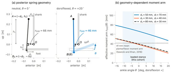
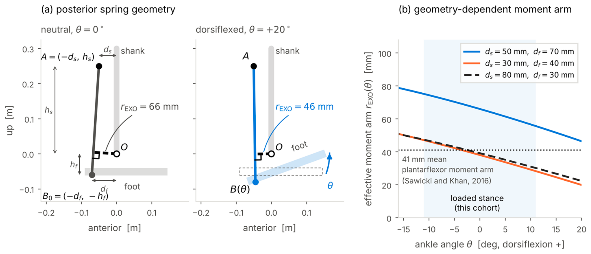
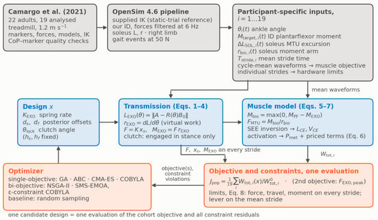
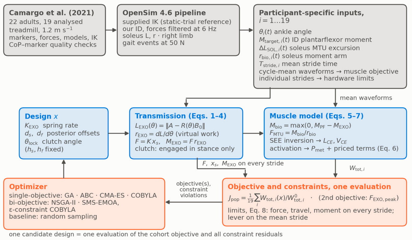
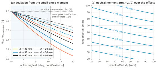
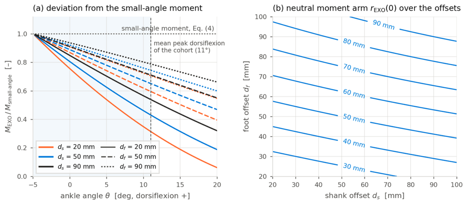
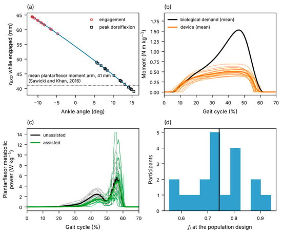
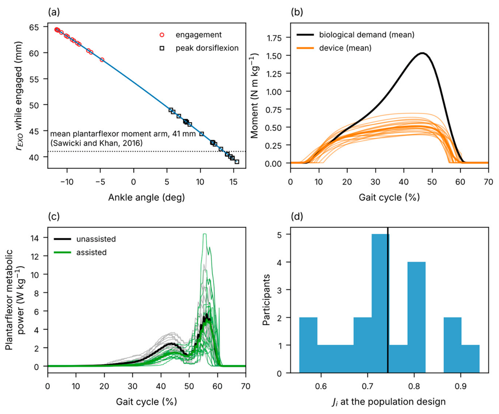
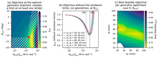
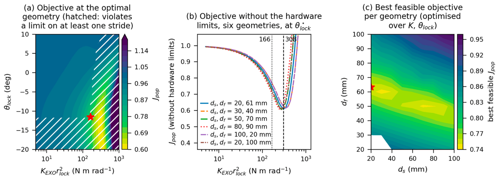
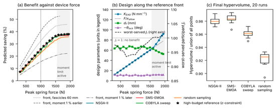
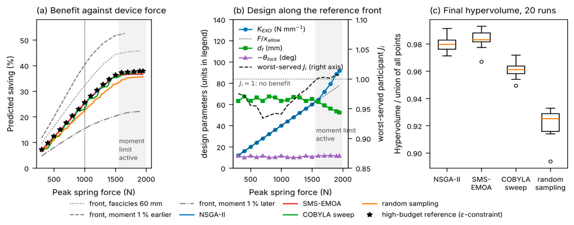
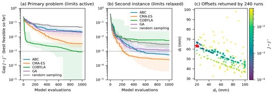
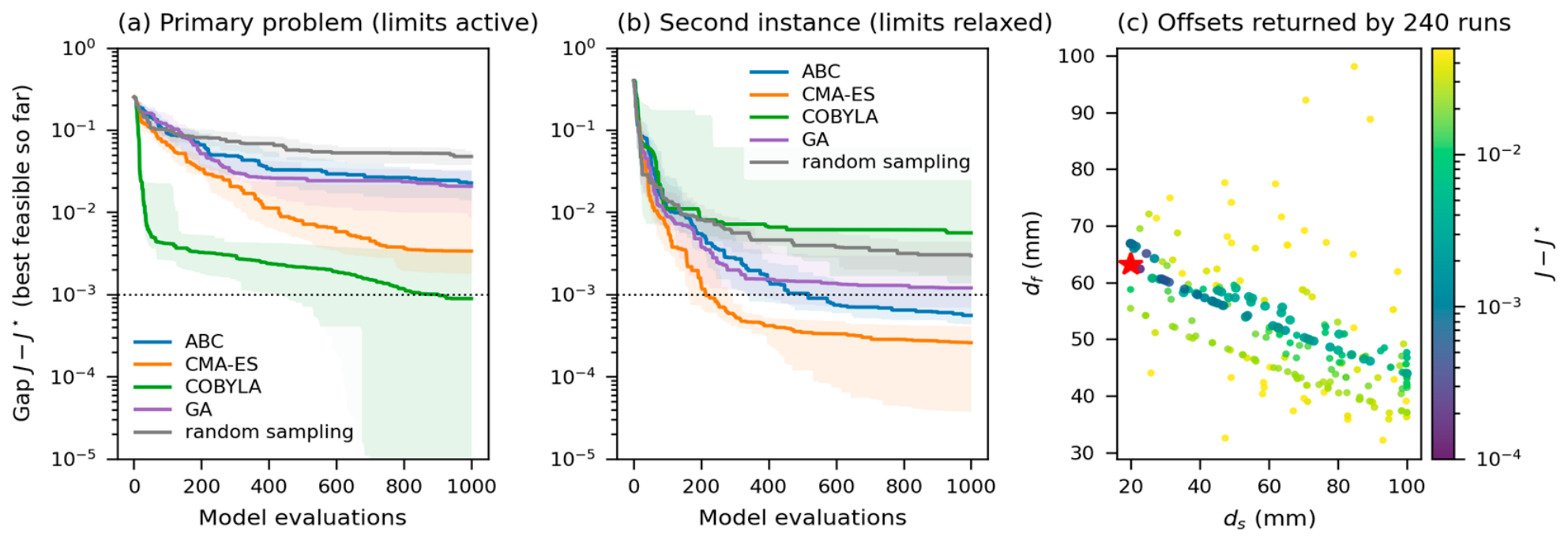

Disclaimer/Publisher’s Note: The statements, opinions and data contained in all publications are solely those of the individual author(s) and contributor(s) and not of MDPI and/or the editor(s). MDPI and/or the editor(s) disclaim responsibility for any injury to people or property resulting from any ideas, methods, instructions or products referred to in the content. |
© 2026 by the author. Licensee MDPI, Basel, Switzerland. This article is an open access article distributed under the terms and conditions of the Creative Commons Attribution (CC BY) license.