


Abstract
We evaluated whether interpretable spatial gaze descriptors discriminate trials from the COCO-Search18 Visual Search dataset and the companion COCO-FreeView dataset while generalizing to participants not used for model fitting. The primary analysis included 45,765 participant-by-image trials from 2094 shared images (20,879 Freeview; 24,886 Visual Search) contributed by two separate 10-participant cohorts. Twelve eye-tracking features representing 10 conceptual families were computed in normalized display coordinates. A Random Forest with a fixed, documented hyperparameter configuration was evaluated using participant-grouped cross-validation. The unadjusted spatial-feature model achieved out-of-fold accuracy 0.9105 and ROC-AUC 0.9632. However, fixation count alone achieved AUC 0.9533, and cumulative recorded fixation duration alone achieved AUC 0.9786, demonstrating strong trial-length differences between the source datasets. After exact fixation-count matching within every validation fold, the count-only negative control returned AUC 0.5000, whereas the spatial-feature model retained mean AUC 0.7999 across 20 matched samples. Thus, spatial gaze descriptors retain residual predictive information after count matching, but the unadjusted performance cannot be attributed to spatial geometry alone. Because the condition is also perfectly confounded with the cohort and acquisition context, the findings do not isolate a causal task-instruction effect.
1. Introduction
Understanding how humans allocate visual attention during scene perception is a central problem in computer vision, cognitive psychology, and human–computer interaction. Eye-tracking technology provides a direct behavioral measure of overt attentional allocation by capturing spatial gaze coordinates over time. Variations in fixation dispersion, spatial clustering, and saccadic amplitude reflect underlying cognitive demands and task constraints. Visual search tasks induce structured, goal-directed scanning patterns, whereas free viewing elicits broader, exploratory gaze distributions [1,2].
Classic theories described spatial attention as a movable spotlight or an adjustable zoom lens [3,4]. Eye movements provide an observable record of overt selection: fixation locations indicate where information was sampled, while the transitions between them reveal how sampling unfolded [5]. Contemporary task-control accounts go further by treating gaze as an active component of information acquisition, continuously coordinated with the observer’s goal and the developing state of the task [6,7].
The modulation of eye movements by cognitive task demands has been well established since Yarbus (1967) [2]. who demonstrated that fixation patterns vary dramatically depending on viewing instructions. Subsequent research confirmed that visual search induces systematic scanning behavior guided by task-relevant features [1,8]. In visual search paradigms, fixations are directed toward likely target locations based on top-down guidance mechanisms [9]. When the target is absent, observers often exhibit broader but strategically structured scanning patterns. In contrast, free viewing is characterized by saliency-driven fixation allocation, influenced by bottom-up image properties [10].
Earlier same-scene work showed that viewing instructions alter eye-movement control during active scene perception [6]. Related naturalistic evidence indicates that where and when people look changes substantially between laboratory and everyday tasks [11]. These results support an active-vision interpretation: gaze is selected to obtain information that is useful for the current goal, rather than being a task-invariant response to image salience alone [7]. Attention-control mechanisms can also contribute differently across tasks: inhibition of return has been framed as facilitating efficient foraging, while novelty-seeking effects vary beyond visual search [12,13].
This task dependence is evident even when the visual input is held constant. Instructions can change which scene regions and objects are selected, as well as fixation count, dwell time, saccade amplitude, and scanpath organization [6,7,11]. A same-image comparison is therefore especially useful here: it reduces gross stimulus-set differences and asks whether the geometry of gaze alone retains a reliable task signature. Several studies have inverted the classic Yarbus question by attempting to predict the instructed task from eye movements. Results have been mixed: Greene et al. were unable to classify four instructed tasks reliably from observers’ eye-movement patterns [14], whereas Henderson et al. successfully classified scene search, scene memorization, reading, and pseudo-reading from multivariate eye-movement features [15]. Borji and Itti also reported successful decoding of seven Yarbus-style tasks [16]. Kardan et al. extended this approach by classifying visual search, scene memorization, and aesthetic preference from distributional properties of fixation durations and saccade amplitudes, with evidence of generalization across participants [17]. Moving beyond discriminative classification, MacInnes et al. used a dynamic Bayesian network to relate instructed tasks, latent cognitive states, and the generation of saccadic vectors [18]. Together, this literature shows both the promise of task inference and the need for careful validation of compact, interpretable gaze features.
Contemporary work has sharpened this distinction by showing that gaze reflects not only stimulus salience but also the observer’s current goal, environmental constraints, and required action. Chen et al. introduced COCO-Search18, a large-scale dataset for target-directed search in natural scenes and demonstrated that target identity and scene context substantially shape fixation selection [19]. Enders et al. subsequently showed in an open-world virtual environment that target instructions increased fixations and dwell time on task-relevant objects, while a concurrent task altered the breadth of scanning [20]. Together, these findings support treating the spatial organization of gaze as a task-sensitive behavioral signal rather than as a stimulus-only response.
Recent computational research has followed two broad routes. One route learns representations directly from raw or transformed scanpaths. For example, Vortmann et al. encoded eye-tracking time series as images and compared conventional summary-feature classifiers with neural models across attentional-state datasets [21]. The other route retains human-interpretable oculomotor summaries and uses supervised learning to infer task or state. Kaczorowska et al. demonstrated interpretable three-way classification of visual and linguistic tasks from eye-movement measures [22]. More recently, Ries et al. showed that fixation- and saccade-related measures can classify changes in naturalistic search demands at the trial level, with complementary information obtained from head movement [23]. These studies establish the feasibility of gaze-based task inference but do not resolve which compact spatial descriptors are sufficient, complementary, and robust to unseen participants.
The present study addresses this question. Deep sequence models capture temporal order but can be sensitive to sample size, preprocessing, and participant-specific patterns. Individual dispersion measures are easier to interpret but describe only particular aspects of gaze. A controlled comparison of global extent, density, central tendency, local clustering, asymmetry, and inter-fixation displacement under subject-disjoint validation is therefore needed. This study addresses that gap by evaluating a common Random Forest pipeline, holding the folds and hyperparameters fixed across full, ablated, and reduced feature sets.
Classifying visual search and free-viewing trials from gaze measurements may help clarify how viewing conditions relate to spatial attention. Such classification may also be useful in adaptive interfaces, workload monitoring, human–AI interaction, and neurocognitive assessment.
Deep learning and temporal sequence models have been used for gaze-based classification, but their learned representations can be difficult to interpret. Spatial dispersion metrics describe specific properties of gaze organization. Measures such as convex hull area, bivariate contour ellipse area (BCEA), nearest neighbor index (NNI), and kernel density–based attention maps quantify the geometry and distribution of fixations in an interpretable manner [24,25].
No single statistic describes all aspects of gaze distribution. Global extent, axis-wise variability, covariance, asymmetry, sequential displacement, local spacing, central tendency, and density concentration describe different aspects of a fixation pattern. They also have different sensitivities to fixation count, outliers, display boundaries, and coordinate scale [26,27]. We therefore evaluated complementary measures using the same preprocessing and coordinate normalization.
This study evaluates the ability of spatial dispersion metrics to distinguish between:
- Freeview Condition
- Visual Search Condition
We used participant-wise GroupKFold cross-validation to prevent trials from the same person appearing in both training and test sets, thereby addressing direct participant-identity leakage. The primary 2094-image analysis yielded an unadjusted OOF ROC-AUC of 0.9632 for distinguishing the two dataset-defined conditions in held-out participants. Because fixation count and cumulative fixation duration differed substantially between datasets, count-matched sensitivity analysis was also required. Neither isolates the effect of task instruction because condition and source cohort are perfectly confounded.
The research questions were:
(RQ1) Can trial-level spatial gaze geometry distinguish between COCO-FreeView trials from COCO-Search18 Visual Search trials for participants not represented during model fitting?
(RQ2) Do HDR68 Area and NNI add complementary predictive information to the remaining descriptors?
(RQ3) Can a reduced dispersion-focused subset retain the performance of the complete feature set?
The contributions of this work are:
- A documented participant-grouped classification framework for the two dataset-defined conditions.
- A controlled ablation study quantifying the contribution of HDR68 Area and NNI.
- Empirical evidence separating unadjusted predictive discrimination from residual spatial-feature discrimination after exact fixation-count matching.
2. Related Work
2.1. Spatial Dispersion Metrics in Eye Tracking
Quantifying gaze dispersion has been approached using multiple geometric measures. Convex hull estimates the spatial extent of fixation distribution [25]. BCEA provides a probabilistic measure of fixation variability by modeling the spatial covariance structure [24]. The nearest neighbor index (NNI), derived from spatial statistics, quantifies clustering versus randomness in point patterns.
The measures can be organized by the property they emphasize. Convex-hull area and bounding-box coverage quantify global extent; horizontal and vertical standard deviations and BCEA summarize second-order spread; skewness captures directional asymmetry; mean saccadic amplitude preserves limited sequential information; NNI describes local spacing; central bias measures displacement from the display centre; and HDR68 Area measures concentration on a common density grid. Ordered scanpath methods such as ScanMatch address sequence similarity more directly [28] but require additional discretization and alignment choices. The present trial-level descriptors are intended as transparent complements to, not replacements for, full temporal scanpath analysis.
Density maps are widely used to represent fixation probability distributions [29]. Here, global attention-map spread was operationalized as the normalized stimulus-image area occupied by the 68% highest-density region after fixed-grid Gaussian smoothing (HDR68 Area), rather than as the integral of a normalized density, which would be approximately constant.
These measures have often been studied separately, but their relative contributions under a common classification procedure remain less well established.
2.2. Machine Learning for Gaze-Based Classification
Machine learning has been applied to eye-movement data for recognizing activities and attentional states. Bulling et al. [30] demonstrated person-independent activity recognition using selected eye-movement features, while more recent studies examined interpretable workload classification [22] and time-series representations [21]. These findings motivate interpretable gaze-feature benchmarking but do not establish that conventional features universally outperform deep learning. Random Forests offer a flexible nonlinear comparator for the present predefined feature sets.
Gaze classifiers must also be evaluated across participants, stimuli, and acquisition contexts. Participant-specific patterns in eye movements have also been studied for biometric recognition [31]. Participant-grouped validation prevents direct reuse of a held-out participant but does not necessarily control cohort or source-specific regularities. Dataset bias can produce apparently strong within-dataset performance that does not transfer beyond the evaluated setting [32]. We therefore interpret the results as a prediction of the two COCO dataset labels, not as an estimate of the causal effect of viewing instructions.
This study uses strict participant-grouped cross-validation to prevent direct identity leakage and to measure prediction for held-out participants. Because each participant contributed data to only one condition, this validation does not separate task effects from cohort or acquisition-context differences.
A directly relevant precedent is Chen et al. (2022) [33], who introduced COCO-FreeView as a companion to COCO-Search18 and examined whether scanpaths could be classified as target-present search, target-absent search, or free viewing using a three-class LSTM model. Their classifier incorporated fixation coordinates and durations together with image-derived visual features. This establishes precedent for predictive classification across these dataset-defined conditions, although it is neither a binary dispersion-feature classifier nor evidence that task effects can be identified independently of participant cohort. In contrast, the present analysis focuses on interpretable trial-level geometry and explicitly evaluates participant- and stimulus-disjoint prediction, fixation-count sensitivity, and clustered uncertainty. Predictive discrimination between the cohorts must not be interpreted as an isolated causal effect of viewing instruction.
3. Methodology
3.1. Overview
This study evaluates whether spatial dispersion metrics derived from eye-tracking data can discriminate between:
- Freeview
- Visual Search
Each trial consists of an ordered set of fixation events:
where (xi, yi) is the two-dimensional coordinate of fixation i, i indexes fixation order, and N is the number of valid fixations in the trial.
G = {(xi, yi)}i=1N
Data Source, Experimental Conditions, and Unit of Analysis
The primary analysis in this study used all valid Visual Search trials, irrespective of response accuracy, because the outcome was viewing condition rather than task success. The 2094 scene images present in both datasets formed the common stimulus set. Data came from two non-overlapping cohorts: 10 COCO-Search18 participants and a separate 10 COCO-FreeView participants. Participant identifiers confirmed that no individual completed both conditions. Consequently, conditions were perfectly aliased with participant cohort and acquisition context. Image matching reduced stimulus-set differences but could not remove this confound. COCO-Search18 participants searched natural scenes for absent target categories; COCO-FreeView participants viewed the corresponding scenes for 5 s without a target cue or response requirement. The unit of analysis was one participant-by-stimulus viewing trial. Trial-level analysis was necessary because convex-hull area, spatial dispersion, HDR68 Area, NNI, BCEA, coverage, and saccadic amplitude summarize multiple fixations within one viewing episode. Treating fixations as independent observations would make most descriptors undefined and would create pseudoreplication. Visual Search trial identity was defined jointly by participant, image, and target category; omitting target category would have collapsed 3398 distinct trial identities. After coordinate filtering, the primary sample contained 45,765 trials: 20,879 Freeview and 24,886 Visual Search. A sensitivity analysis corresponding to the original eligibility rule restricted Visual Search to correct responses, producing 43,381 trials from 2077 shared images (20,710 Freeview; 22,671 Visual Search). It was treated as a robustness check rather than the primary estimate.
The original COCO-Search18 sample comprised 10 participants (six male and four female), aged 18–30 years, with self-reported normal or corrected-to-normal vision. They were naive to the task design at recruitment and received course credit or monetary compensation. Participants provided informed consent under a protocol approved by the Stony Brook University Institutional Review Board. Each participant completed approximately 12 h of testing over six days. The companion COCO-FreeView sample consisted of 10 university students who viewed images for 5 s in anticipation of a memory test; each participant completed approximately 12 h over six sessions. The published dataset description reports eye-position recording at 1000 Hz using an EyeLink 1000 (SR Research Ltd., Ottawa, ON, Canada) and offline fixation extraction with default settings; institutional ethics approval and informed consent were reported [33]. COCO-FreeView participant demographics beyond the source description are not inferred here. These documented similarities do not establish identical calibration criteria, head stabilization, viewing distance, or every acquisition setting across the two cohorts.
3.2. Preprocessing and Quality Control
The released files contained fixation-level events rather than raw gaze samples; therefore, no new velocity-, acceleration-, dispersion-, or minimum-duration fixation detector was applied. Source-row order was retained as the fixation order. The analysis was restricted to the 2094 image files present in both datasets. Rows were eligible when image name, participant identifier, X coordinate, and Y coordinate were observed; Visual Search trial construction additionally required target category. Visual Search trials were keyed by participant, image, and target category, whereas Freeview trials were keyed by participant and image. The primary analysis retained Visual Search trials irrespective of response correctness; the correct-response filter was used only in the sensitivity analysis. Coordinates outside the inclusive display domain 0 ≤ X ≤ 1680 pixels and 0 ≤ Y ≤ 1050 pixels, were discarded. Retained coordinates were normalized as x = X/1680 and y = Y/1050, and a trial was modelled when at least one valid on-screen fixation remained. Coordinates were neither imputed nor pooled across trials.
We applied fixed rules for descriptors when a trial contained too few fixations for the usual calculation. For a one-fixation trial, convex-hull area, horizontal and vertical standard deviations, horizontal and vertical skewness, mean saccadic amplitude, FVF, BCEA, and bounding-box coverage were 0; NNI was assigned its neutral value of 1; HDR68 Area and central bias were computed from the observed fixation. For a two-fixation trial, convex-hull area, both skewness terms, and BCEA were 0, while the remaining descriptors were computed normally. For trials with at least three fixations, a convex-hull failure caused by degenerate geometry returned 0, and any negative covariance determinant was truncated to 0 before the BCEA square root. After calculation, any remaining non-finite descriptor was mapped to 0, except NNI, which was mapped to 1. We verified that all feature values were finite before fitting the models.
In the original COCO-Search18 acquisition, gaze was recorded with an EyeLink 1000 (SR Research Ltd., Ottawa, ON, Canada) in tower-mount configuration at 1000 Hz. Images were displayed on a 22-inch LCD monitor at 1680 × 1050 pixels, viewed from 47 cm with chin and head rests, subtending approximately 54° × 35°. Nine-point calibration was performed before each block or when necessary and was accepted only when the mean error was ≤0.51° and the maximum error was ≤0.94°. The experiment was conducted in a quiet, dimly lit laboratory. The dataset authors clustered approximately 70 million raw gaze samples into 299,037 search fixations and excluded fixations from incorrect trials, leaving 268,760 search fixations. Because this study analyzed the released fixation tables, these are source-dataset procedures, not thresholds newly applied by the present analysis [19].
3.3. Fixation-Count and Cumulative-Duration Sensitivity Analyses
The released T field was treated as fixation duration in milliseconds. For each reconstructed trial, fixation count was the number of retained fixation events, and cumulative recorded fixation duration was the sum of T across those events. This sum was not treated as complete trial duration because it excludes saccades, response time, and other non-fixation intervals. Trial-level distributions were summarized separately for Freeview, correct Visual Search, and incorrect Visual Search trials. Nuisance-only Random Forest baselines used fixation count alone, cumulative fixation duration alone, or both variables, with the same participant folds and hyperparameters as the spatial-feature model.
For the matched analysis, trials were stratified jointly by validation fold, integer fixation count, and condition. Within each validation fold, trials were grouped according to their exact integer fixation count. For each fixation-count group, an equal number of Free Viewing and Visual Search trials were retained by randomly undersampling the condition containing more trials. Consequently, the two conditions had identical fixation-count distributions within each fold. This made the fixation-count distribution identical between conditions in every held-out fold and in its complementary training set. Matching was repeated for 20 seeds (42–61), while participant fold membership and model hyperparameters remained fixed. The complete 12-feature model was evaluated on each matched sample. A matched fixation-count-only negative control verified that the matching removed all discriminative information from the count. The correct-response-only 2077-image dataset was processed identically as a sensitivity analysis.
In a further sensitivity analysis, trials were jointly matched within each participant-validation fold by exact integer fixation count and cumulative recorded fixation-duration bands of 250 ms. Within each fold-by-count-by-duration stratum, the condition with more trials was randomly undersampled to match the smaller condition; strata without trials from both conditions were excluded. Twenty repetitions used matching seeds 42–61, with unchanged participant folds, 12 spatial predictors, and Random Forest hyperparameters. A duration-only classifier evaluated remaining information in continuous cumulative fixation duration on the same matched trials. A secondary check used 500-ms bands over five matching seeds (Supplementary Table S5).
To assess response-accuracy filtering separately from the change in image set, we compared both eligibility rules on the same 2077 images. For each of 20 matching seeds, the all-trial and correct-only arms used the same participant-fold assignment, identical selected Freeview trials, equal class sizes, and identical fixation-count distributions within every validation-fold-by-count stratum. Each arm contained 6682 trials per repetition (3341 per condition). Seed-level differences were summarized descriptively because the repeated matched samples overlap and are not independent experiments.
3.4. Dispersion-Based Feature Extraction
Ten conceptual gaze-descriptor families were computed per trial, yielding 12 numeric variables because standard deviation and skewness were each calculated separately for the horizontal and vertical coordinates.
These features describe several aspects of spatial gaze distribution. Global extent was represented by convex-hull area, BCEA, functional viewing field, bounding-box coverage, axis-specific standard deviations, and the 68% highest-density region area (HDR68 Area); location relative to the actual display center by central bias; shape by axis-specific skewness; local point-pattern organization by NNI; and movement between successive fixations by mean saccadic amplitude. All quantities were calculated independently for each trial in normalized display coordinates. Figure 1 illustrates four of these descriptors.
Figure 1.
Visual explanation of four complementary trial-level measures using one correct-response visual-search trial with 18 fixations: (A) the radial FVF-area proxy, with radius SD(r); (B) the 68% BCEA; (C) coverage as the axis-aligned fixation bounding-box area divided by the normalized display area; and (D) HDR68 Area on the fixed 50 × 32 Gaussian-smoothed grid, with the smallest set of cells containing at least 68% of density outlined and the corresponding density surface inset. For this illustrative trial, 94 of 1600 grid cells were selected (HDR68 Area = 0.05875). Blue points denote fixation locations, the green circle illustrates the radial FVF proxy, the red ellipse denotes BCEA, the orange rectangle shows bounding-box coverage, and the white contour outlines the HDR68 Area.
The convex-hull area was the area of the smallest convex polygon enclosing all valid fixation locations. Standard deviation was computed separately for the horizontal and vertical coordinates. Skewness was likewise computed separately for X and Y using the scipy.stats.skew function (SciPy version 1.17.0). Mean saccadic amplitude was defined as the mean Euclidean distance between successive fixation locations. The axis-specific standard-deviation and skewness terms explain why the complete design matrix can contain 12 numeric columns while representing 10 conceptual descriptor families. The archived primary-analysis environment records Python 3.12.14, NumPy 2.3.5, pandas 2.2.3, SciPy 1.17.0, and scikit-learn 1.8.0.
The functional viewing field (FVF) was computed from the radial distances between the fixations and the trial centroid. For fixation i, ri is this radial distance; SD(r) is the population standard deviation of the N radial distances; and FVF = π[SD(r)]2. Central bias was defined as the mean Euclidean distance from each fixation to the normalized stimulus center (0.5, 0.5). BCEA used the covariance eigenvalues and the 68% chi-square constant, 2.278868566. Bounding-box coverage was the axis-aligned fixation bounding-box area divided by the full stimulus-image analysis area.
The normalized 68% highest-density region area (HDR68 Area) was computed on a fixed 50 × 32 grid covering the stimulus image in normalized coordinates. This resolution approximately preserves the 1680 × 1050 image-display aspect ratio while providing a reproducible compromise between spatial detail and sparse cell counts; it was an implementation choice, not an optimized or preregistered parameter. Fixation counts were Gaussian-smoothed with σ = 1 grid cell and normalized to unit mass. Here, σ is the Gaussian-kernel standard deviation: one grid cell, approximately 33.6 horizontal pixels and 32.8 vertical pixels. Smoothing distributes fixation mass to neighboring cells and reduces grid-boundary and isolated-cell noise. Cells were ranked by smoothed density, and the smallest set containing at least 68% of the total fixation-density mass was identified. HDR68 Area is the area of that cell set divided by the area of the complete 50 × 32 stimulus grid. It therefore reports how much of the image plane contains the central 68% of a trial’s smoothed gaze distribution; it does not refer to the physical monitor area. NNI compares the observed mean nearest-neighbour distance among fixations with the expected distance under complete spatial randomness over the same normalized image plane.
Figure 2 illustrates this measure using the mean Freeview fixation-density map. HDR68 Area is the proportion of grid cells needed to contain 68% of the smoothed mass; smaller values indicate a more concentrated attention map.
Figure 2.
Equal-trial-weight mean Freeview fixation-density map from 20,879 trials over 2094 shared images. The 68% highest-density region occupies 371 of 1600 grid cells (normalized HDR68 Area = 0.231875, or 23.19% of the image plane). This map-level statistic differs from the mean individual-trial HDR68 Area (0.041833). The white line outlines the region containing 68% of the averaged fixation-density mass.
To assess HDR68 Area parameter sensitivity, we used a participant-balanced subset of 3000 trials. Grid resolution, Gaussian smoothing width, and cumulative density threshold were varied individually, with the remaining predictors and Random Forest settings held constant.
Classification performance was evaluated using five-fold participant-grouped cross-validation. The configurations and corresponding results are provided in Supplementary Table S4.
(1) Convex Hull Area (CHA)
CHA = Area[ConvexHull(G)]
CHA measures the area enclosed by the outermost fixation points, providing an estimate of the spatial extent of gaze exploration. Larger values indicate that gaze extends across a wider portion of the normalized display, whereas smaller values indicate greater spatial concentration. Because the boundary is determined by extreme points, CHA is sensitive to isolated peripheral fixations and to trials with few fixations; it should therefore be interpreted alongside covariance- and density-based measures.
(2) Standard Deviation (STD)
Overall dispersion magnitude:
Axis-wise standard deviations retain directional information that a single area measure discards. They distinguish predominantly horizontal from predominantly vertical spread, but they do not encode the orientation of an oblique fixation cloud or its boundary shape. Normalized coordinates make both quantities comparable across the common display geometry.
(3) Skewness (SKEW)
Axis-specific spatial asymmetry (computed separately for q = x and q = y):
The sign of skewness indicates the direction of the longer tail on each axis; values near zero indicate approximate symmetry. The sample-skewness form in Equation 4 is transparent and scale-free [34]. Skewness is nevertheless sensitive to extreme fixations and becomes unstable when an axis has negligible variance.
(4) Saccadic Amplitude (SA)
SA = (1/(N − 1)) Σi=1N−1 √{(xi+1 − xi)2 + (yi+1 − yi)2}
This measure is the mean Euclidean displacement between consecutive recorded fixations, expressed in normalized-image units. It therefore retains a limited aspect of temporal order: large values indicate broader steps through the scene, whereas small values indicate locally concentrated transitions [11]. It is a scanpath displacement measure, not a velocity measure, because fixation-to-fixation time is not included.
(5) Functional Viewing Field (FVF)
Here, N is the number of valid fixations in the trial; (xi, yi) is fixation i in normalized image coordinates; (, ȳ) is the trial centroid; ri is the Euclidean distance from fixation i to that centroid; and SD(r) is the population standard deviation of {r1, …, rN}. The FVF is expressed as a proportion of the normalized image area.
In this manuscript, FVF is an operational radial-area proxy derived from the dispersion of fixation distances around their centroid; it is not a direct psychophysical estimate of the observer’s functional visual field. Classical functional-field-of-view work concerns the region over which useful information can be acquired under specified perceptual and attentional demands [35,36,37]. The present proxy is retained as a compact summary of radial spread and interpreted only in that statistical sense.
(6) Normalized 68% Highest-Density Region Area (HDR68 Area)
Let cuv be the fixation count in cell (u, v) of a fixed 50 × 32 normalized stimulus-image grid. The grid approximately preserves the display aspect ratio. Counts were convolved with a Gaussian kernel having standard deviation σ = 1 grid cell; this corresponds to approximately 33 pixels in either display direction and reduces discretization noise. The grid size and smoothing width were fixed implementation choices and were not optimized against the outcome.
Let pj denote the normalized density mass in grid cell j, with Σj pj = 1. Thus, j is a subscript indexing grid cell. Cells were sorted from highest to lowest density.
After ranking the cells so that p1 ≥ p2 ≥ …, we defined m* as the smallest number of cells containing at least 68% of the mass. This is not the integral of the normalized map, which equals 1.
pᵤᵥ = [K(σ) * c]uv/Σα=150 Σβ=132 [K(σ) * c]αβ, σ = 1
m* = min{m:Σj=1ᵐ pj ≥ 0.68}; HDR68 Area = m*/(50 × 32)
In Equations (7) and (8), cuv is the fixation count in grid cell (u, v); K(σ) is the Gaussian smoothing kernel; * denotes two-dimensional convolution; puv is the normalized smoothed mass in cell (u, v); pj is the same mass after cells have been ranked so that p1 ≥ p2 ≥ …; m* is the smallest number of highest-density cells whose cumulative mass reaches 0.68. The denominator 50 × 32 is the total number of grid cells covering the stimulus image.
HDR68 Area is relative to the complete stimulus-image grid: it is the proportion of that image plane required to contain 68% of the trial’s smoothed fixation-density mass. Smaller values indicate a more concentrated gaze distribution.
(7) Nearest Neighbor Index (NNI)
Observed and expected nearest-neighbour distances were defined as follows:
d(obs) = (1/N) Σi=1N minl≠i ||zi − zl||2
d(exp) = 0.5√(A/N)
NNI = d(obs)/d(exp)
In Equations (9)–(11), zi = (xi, yi); ||·||2 is Euclidean distance; minl≠i selects the nearest other fixation to fixation i; d(obs) is the observed mean nearest-neighbour distance; d(exp) is the expected mean distance under complete spatial randomness; N is the number of fixations; and A is the normalized image-plane area, equal to 1.
NNI compares observed nearest-neighbour spacing with the expectation under complete spatial randomness on the unit-area normalized display. Values below 1 indicate clustering, values near 1 approximate spatial randomness, and values above 1 indicate more regular spacing. Like other point-pattern statistics, NNI depends on fixation count and boundary effects, which is why it is evaluated under the same trial construction and coordinate support throughout.
(8) Bivariate Contour Ellipse Area (BCEA)
where χ20.68,2 = 2.278868566 and λ1 and λ2 are the covariance-matrix eigenvalues.
BCEA68 = πχ20.68,2 √(λ1λ2)
BCEA is a covariance-based ellipse summary: the covariance eigenvalues determine spread along the principal axes, while their eigenvectors determine orientation. The 68% choice provides an interpretable probability-region summary for a bivariate normal fixation cloud [38]. BCEA is less boundary-focused than CHA, but its elliptical summary can underrepresent multimodal or strongly non-Gaussian patterns.
(9) Central Bias (CB; Distance From Display Centre)
CB = (1/N) Σi=1N √{(xi − 0.5)2 + (yi − 0.5)2}
Central bias is referenced to the geometric center of the normalized display, not to an object, saliency peak, or scene-specific region of interest. Smaller values indicate that the mean fixation-to-center distance is lower. This measure is useful because scene viewing often exhibits a central fixation tendency [39].
(10) Coverage (COV)
COV = [(x(max) − x(min))(y(max) − y(min))]/A
In Equation (14), x(min), x(max), y(min), and y(max) are the extrema of the trial’s fixation coordinates. A is the area of the full stimulus-image analysis domain. Because coordinates were normalized to [0, 1] × [0, 1], A = 1; coverage is therefore the fraction of the image plane enclosed by the fixation bounding box (Figure 1).
Here, coverage is strictly the area of the axis-aligned fixation bounding box divided by the full normalized display area A = 1. It is therefore a global extent measure, not object coverage, target coverage, or the proportion of semantically meaningful scene content inspected. It is simple and interpretable, but a single peripheral fixation can expand the box substantially.
Classification Model
Random Forest classifier:
where x is the trial-level feature vector, Tk(x) is the class predicted by tree k, k indexes the 200 trees, mode selects the majority class, and ŷ(x) is the ensemble prediction.
ŷ(x) = mode{Tk(x):k = 1, …, 200}
Hyperparameters:
All full and ablation models used scikit-learn version 1.8.0 RandomForestClassifier with 200 trees, maximum depth 15, minimum samples per split 5, minimum samples per leaf 2, class_weight = “balanced”, random_state = 42, and n_jobs = 1. Unspecified settings used scikit-learn defaults: Gini criterion, max_features = “sqrt”, bootstrap = True. The identical estimator configuration and participant folds were used for every feature-set comparison. The number of trees provides an ensemble of moderate size, depth, and leaf constraints limit tree complexity, balanced class weights address unequal trial counts, and seed 42 ensures repeatability.
Five-fold GroupKFold was applied without shuffling, using participant ID as the grouping variable. For each fold, the model was fitted only to trials from training participants, and probabilities and labels were generated only for held-out participants. These foldwise predictions were concatenated once to obtain the pooled OOF confusion matrix, classification report, accuracy, balanced accuracy, and ROC-AUC. The ablation analysis, rather than a full-data feature-importance ranking, was used to quantify the incremental predictive contribution of the specified descriptors.
3.5. Stimulus-Disjoint and Crossed Participant–Image Validation
To evaluate the influence of scene-image overlap, we conducted two additional out-of-fold validation experiments on the existing 12-feature trial-level matrices, without recalculating descriptors or tuning classifier settings. Images were assigned to five non-overlapping groups using a seeded permutation (random state = 42) of the 2094 image identifiers; the 2077-image sensitivity sample retained these same image-group assignments. Five participant groups were constructed, each containing two Freeview and two Visual Search participants, using seed 42. These supplementary splits were generated separately from the original participant GroupKFold evaluation.
In five-fold image-disjoint validation, each model was trained on trials from four image groups and tested on the fifth. Individual participants could appear in both sets; therefore, this analysis tested stimulus independence only. In crossed participant–image validation, 25 models were fitted for the five-by-five combinations of held-out participant and image groups. For each evaluation, the model was trained without data from the selected participant and image groups and then tested on trials involving both held-out groups. Every trial was evaluated exactly once, and neither the test participant IDs nor test image IDs appeared in the corresponding training set. All repetitions of an image were grouped by the canonical image filename, regardless of Visual Search target category.
Both procedures used RandomForestClassifier with 200 trees, maximum depth 15, min_samples_split = 5, min_samples_leaf = 2, class_weight = balanced, random_state = 42, n_jobs = 1, and otherwise default scikit-learn settings. We report pooled out-of-fold accuracy, balanced accuracy, and ROC-AUC. The primary analysis used 45,765 trials from 2094 overlapping images; the correct-response sensitivity sample used 43,381 trials from 2077 images. The analysis assesses predictive discrimination across the two dataset-defined cohorts, not an isolated causal effect of task instructions.
3.6. Controlled Ablation Framework
To quantify the contribution of HDR68 Area and NNI, controlled ablation experiments were conducted under identical subject-wise cross-validation splits and identical model hyperparameters.
Let the full feature set be:
where:
F(full) = {f1, f2, …, f10}
F(full) = {CHA, STD, SKEW, SA, FVF, HDR68 Area, NNI, BCEA, CB, COV}
(1) HDR68 Area Removal
F(−HDR68 Area) = F(full)\{HDR68 Area}
Performance difference:
where M(·) denotes the selected held-out performance metric, either accuracy or ROC-AUC.
Δ(HDR68 Area) = M[F(full)] − M[F(−HDR68 Area)]
(2) NNI Removal
F(−NNI) = F(full)\{NNI}
Δ(NNI) = M[F(full)] − M[F(−NNI)]
(3) Single-Feature Models
F(HDR68 Area) = {HDR68 Area}
F(NNI) = {NNI}
(4) Dispersion-Only Subset
F(disp) = {CHA, STD, HDR68 Area, NNI, BCEA, CB, COV}
All ablation models were evaluated using identical subject-wise folds:
M(Fk) = (1/K) Σj=1ᴷ Accuracyj, K = 5
All models used the same five participant-grouped folds.
Selection and Composition of the Reduced Feature Set
The eight predictor columns were convex-hull area, horizontal and vertical standard deviations, HDR68 Area, NNI, BCEA, central bias, and bounding-box coverage. They were grouped conceptually as measures of spatial spread, density concentration, local spacing, covariance, and central tendency. The excluded columns were horizontal and vertical skewness, mean saccadic amplitude, and FVF area, representing asymmetry, sequential displacement, and radial spread. The reduced feature set was therefore assessed as an exploratory alternative rather than as a model specified in advance.
3.7. Evaluation Metrics
For binary classification:
Accuracy was the proportion of correctly classified observations. Precision, recall, and F1 were computed separately for each class; macro F1 assigned equal weight to the two classes, whereas weighted F1 weighted class-specific values by support. ROC-AUC was computed from held-out visual-search probabilities [40] and measures performance ranking across all possible thresholds. The confusion matrix and classification report used the default decision threshold of 0.50.
Accuracy = (TP + TN)/(TP + TN + FP + FN)
Precision = TP/(TP + FP)
Recall = TP/(TP + FN)
F1 = 2(Precision × Recall)/(Precision + Recall)
ROC-AUC:
AUC = ∫01 TPR(FPR) dFPR
ΔM(f) = M[F(full)] − M[F(−f)]
Participant-Level and Hierarchical Uncertainty
Because trial observations were nested within participants and repeated scene images, we evaluated uncertainty using the original out-of-fold (OOF) predictions rather than treating all trials as independent replications. For each participant, we calculated the number of evaluated trials, own-class recall (equivalent to accuracy for a single-condition participant), and mean probability assigned to the participant’s observed condition. Individual-participant ROC-AUC is not identifiable because each participant supplied observations from only one condition.
We calculated two percentile-bootstrap sensitivity analyses with 1000 replicates (random seed 20261017). The first resampled 10 participant IDs with replacement independently within each condition and retained all associated trials using cluster multiplicity weights. The second independently resampled participant IDs within condition and scene IDs, then multiplied participant and image resampling weights at the trial level (crossed, multiway-cluster bootstrap). For each replicate we recomputed pooled ROC-AUC, accuracy, and balanced accuracy using the observation weights. Reported intervals are the 2.5th and 97.5th percentiles. For the count-matched and joint count-and-duration-matched spatial models, participant-cluster uncertainty was additionally calculated for the mean ROC-AUC across all 20 repeated matched selections. In each of 10,000 bootstrap replicates, participants were resampled with replacement independently within each condition, using the same resampled participant identities across all 20 selections. For each selection, pooled held-out ROC-AUC was recomputed using cluster multiplicity weights and then averaged across selections. Percentile 95% intervals quantify participant-level uncertainty conditional on the existing trained models and cohorts; they do not include model retraining or external-cohort variation (Supplementary Table S6).
3.8. Reproducibility and Reporting
The analysis code and aggregate results supporting this study are deposited with Zenodo under DOI https://doi.org/10.5281/zenodo.24157956 (accessed on 12 November 2026). The archive includes scripts for feature extraction, participant-grouped and image-disjoint validation, feature ablation, fixation-count and cumulative-duration matching, HDR68 Area sensitivity analysis, and participant-cluster bootstrap estimation, together with aggregate results and execution instructions. The original COCO-Search18 and COCO-FreeView datasets, derived trial-level feature matrices, and trial-level predictions are not redistributed. Reproducing the analyses therefore requires obtaining the original datasets and reconstructing the necessary intermediate inputs using the accompanying code and instructions.
4. Results
4.1. Subject-Wise Classification Performance
Performance was evaluated with five-fold GroupKFold using participants as the grouping variable. Every trial-level prediction was generated by a model that had not been trained on that participant. These estimates quantify held-out-participant prediction between the two source cohorts; they do not identify a task effect independently of cohort.
4.2. Fixation Count and Cumulative Fixation Duration
Freeview trials contained a mean of 15.44 fixations (SD 3.24; median 16), compared with 5.87 (SD 4.06; median 5) for correct Visual Search trials and 5.78 (SD 3.73; median 5) for incorrect Visual Search trials. Mean cumulative recorded fixation duration was 4053 ms (SD 526) for Freeview, 1264 ms (SD 939) for correct Visual Search, and 1459 ms (SD 1017) for incorrect Visual Search. Figure 3 shows the marked separation of the distributions.
Figure 3.
Trial-Level Fixation-Count and Cumulative Recorded Fixation-Duration Distributions.
In the primary 2094-image dataset, fixation count alone achieved OOF AUC 0.9533, cumulative recorded fixation duration alone achieved AUC 0.9786, and their combination achieved AUC 0.9842. These control analyses show that simple fixation summaries carry substantial information about the dataset-defined condition. They do not determine whether spatial descriptors retain information beyond fixation count; this was tested directly using exact-count matching.
Fold-wise exact count matching retained 7086 trials per repetition in the primary analysis. Across 20 matched samples, the 12-feature model achieved a mean accuracy of 0.7314 ± 0.0048 and a mean ROC-AUC of 0.7999 ± 0.0046 (range 0.7940–0.8083). The matched count-only negative control returned accuracy, balanced accuracy, and AUC of 0.5000 in every repetition. In the correct-response-only 2077-image sensitivity analysis, 6674 matched trials were retained per repetition, and the spatial model achieved a mean AUC of 0.8079 ± 0.0039. Table 1 summarizes the unadjusted, nuisance-only, and matched results.
Table 1.
Trial-Length Baselines and Exact-Count-Matched Sensitivity Results.
In the exploratory joint count-and-duration sensitivity analysis, 250-ms duration-band matching retained 3062 trials per repetition (6.7%) in the primary 2094-image sample. Across 20 repetitions, spatial ROC-AUC was 0.8016 ± 0.0059 (mean ± SD), and accuracy was 0.7351; the continuous-duration-only baseline yielded an ROC-AUC of 0.5159. In the 2077-image correct-response sensitivity sample, 2800 trials per repetition (6.5%) were retained, with spatial ROC-AUC 0.8042 ± 0.0075, accuracy 0.7381, and duration-only ROC-AUC 0.5203. A supplementary 500-ms-band check is reported in Supplementary Table S5. The matching repetitions overlap and do not constitute independent samples.
Participant-stratified bootstrap intervals based on all 20 matched selections were 0.7297–0.8485 for the primary exact-count-matched mean AUC (0.7999) and 0.7201–0.8484 for the primary jointly matched mean AUC (0.8016). Corresponding intervals in the 2077-image correct-response sensitivity dataset were 0.7459–0.8504 (mean AUC 0.8079) and 0.7255–0.8557 (mean AUC 0.8042). All 20 participants were represented in every matched selection, although participant contributions were unequal. In the primary 2094-image sample, the number of trials retained per participant in individual matched selections ranged from 45 to 962 under exact fixation-count matching and from 9 to 510 under joint count-and-duration matching. The corresponding ranges in the 2077-image correct-response sample were 41–915 and 6–462, respectively. The intervals reflect participant variation, whereas the reported between-seed SDs describe variation in selected trials (Supplementary Table S6).
The correct-response-only benchmark used 43,381 trials from 2077 shared images and yielded unadjusted participant-disjoint ROC-AUC 0.9616 (see the comparative results in Section 4.6). A separate diagnostic comparison restricted both eligibility rules to the same 2077 images and then matched their selected Freeview observations, participant folds, trial counts, and fixation-count distributions. Each matched arm contained 6682 trials per repetition. Across 20 repetitions, mean spatial AUC was 0.8020 ± 0.0045 with all Visual Search trials eligible and 0.8095 ± 0.0041 with correct responses only, a mean descriptive difference of 0.0075. The all-trial samples included a mean of 264 incorrect Visual Search trials per repetition (range 255–275), and the count-only negative control remained at AUC 0.5000. These matched diagnostic AUCs are not the unadjusted 2077-image benchmark, and the overlapping matching repetitions are not independent samples.
The preprocessing audit found no rows with missing image, participant, X, or Y fields in the 2094-image analysis set. Thirty-four Visual Search fixation rows and no Freeview rows lay outside the recorded display; their removal did not eliminate any trial. The resulting 45,765-trial feature matrix contained no non-finite values. Low-sample conventions applied to 49 of 20,879 Freeview trials (22 with one fixation and 27 with two) and 2090 of 24,886 Visual Search trials (164 with one fixation and 1926 with two). No convex-hull failures, non-finite skewness values, non-finite covariance determinants, or negative covariance determinants occurred among trials with at least three fixations. As a diagnostic sensitivity analysis, excluding all trials with fewer than three valid fixations left 43,626 trials (20,830 Freeview; 22,796 Visual Search) and produced OOF accuracy of 0.9034, balanced accuracy of 0.9046, and ROC-AUC of 0.9598, compared with 0.9105, 0.9124, and 0.9632 in the primary analysis. Thus, the deterministic low-sample conventions did not account for the high unadjusted discrimination.
Across 45,765 held-out trials, the confusion matrix contained 19,515 correctly classified Freeview trials, 1364 Freeview trials classified as Visual Search, 2733 Visual Search trials classified as Freeview, and 22,153 correctly classified Visual Search trials. Thus, 41,668 trials were classified correctly and 4097 incorrectly, giving pooled OOF accuracy of 0.9105 (Figure 4).
Figure 4.
Confusion Matrix for Primary 2094-Image Analysis (OOF Predictions).
The Visual Search class was more prevalent (24,886/45,765); a classifier that always predicted that majority class would achieve 0.5438 accuracy. The full model exceeded this baseline by 0.3667. Macro F1 was 0.9102, and weighted F1 was 0.9106 (Table 2).
Table 2.
Class performance.
- Mean fold accuracy: 0.9105 ± 0.0304
- OOF accuracy: 0.9105; balanced accuracy: 0.9124
- OOF ROC-AUC: 0.9632
4.3. Class-Level Performance
Overall metrics:
Accuracy: 0.9105
Macro F1-score: 0.9102
Weighted F1-score: 0.9106
4.4. ROC Performance
Figure 5 presents the participant-disjoint receiver operating characteristic (ROC) curve.
Figure 5.
ROC Curve for Primary 2094-Image Analysis Under Participant-Wise Cross-Validation. The dotted diagonal represents chance-level discrimination (ROC-AUC = 0.50).
The participant-disjoint OOF ROC-AUC was 0.9632: within the combined primary dataset, a randomly selected Visual Search trial received a higher Visual Search score than a randomly selected Freeview trial approximately 96.3% of the time. This threshold-independent result complements the confusion matrix at the default 0.50 threshold. It is an unadjusted discrimination estimate and should not be interpreted as spatial information independent of fixation count or as a task effect separated from cohort.
ROC-AUC = 0.9632
4.5. Controlled Ablation Study
Controlled ablation experiments used identical participant folds and Random Forest hyperparameters. Table 3 presents pooled out-of-fold (OOF) accuracy and ROC-AUC, alongside the mean and standard deviation of accuracy across folds, allowing descriptive comparisons of model performance. Table 4 summarises performance across the validation designs, and Table 5 compares the Random Forest and logistic regression results. Paired uncertainty for the HDR68 Area and NNI ablation contrast is reported in Supplementary Table S3. The paired comparison provided insufficient evidence that the reduced feature model outperformed the full model.
Table 3.
Subject-Wise Ablation Results for the Primary 2094-Image Analysis.
Table 4.
Participant-disjoint, image-disjoint, and crossed participant–image-disjoint out-of-fold performance. Values are pooled over the respective held-out predictions; these evaluations were not fixation-count or duration matched.
Table 5.
Comparison of Random Forest and Logistic Regression Classification Performance Across the 2094-Image and 2077-Image Datasets.
4.6. Performance Differences
Performance changes relative to the full model were:
Removing the HDR68 Area reduced the primary pooled OOF ROC-AUC from 0.963247 to 0.959157 (ΔAUC = 0.004090); removing NNI reduced it to 0.952435 (ΔAUC = 0.010812). The corresponding accuracy reductions were 0.006512 and 0.015820, respectively. We evaluated the difference between these ablation effects using paired participant-aware uncertainty, as detailed below.
The HDR68 Area-only model achieved accuracy 0.8199 and AUC 0.8812; the NNI-only model achieved accuracy 0.6160 and AUC 0.6597. Both were below the multivariable models. The eight-feature dispersion subset produced accuracy 0.9113, balanced accuracy 0.9131, AUC 0.9646, and fold accuracy 0.9113 ± 0.0302. Relative to the full model, its numerical differences were +0.0009 accuracy and +0.0014 AUC.
These ablation comparisons estimate the contribution of each descriptor conditional on the remaining features and the fixed Random Forest configuration. A paired participant-bootstrap comparison was performed for the eight-feature reduced and twelve-feature full models (see “Paired full-versus-reduced feature comparison”). The small reduced-minus-full AUC difference was not statistically reliable, and the superiority of the reduced model is not established.
ΔAUC(HDR68 Area) = 0.963247 − 0.959157 = 0.004090
ΔAUC(NNI) = 0.963247 − 0.952435 = 0.010812
Accuracy differences:
ΔAccuracy(HDR68 Area) = 0.910477 − 0.903966 = 0.006512
ΔAccuracy(NNI) = 0.910477 − 0.894657 = 0.015820
Single-feature models performed substantially below every multivariable configuration.
4.7. Paired Ablation Uncertainty Analysis
We regenerated held-out probabilities from the HDR68 Area-removed and NNI-removed models using the five participant-grouped folds, fixed 200-tree Random Forest, and existing trial-level predictor tables. Their pooled AUC values reproduced the original ablation table. Full-model probabilities were retained from the original analysis. We calculated a paired ablation contrast as [AUC(full) − AUC(without NNI)] − [AUC(full) − AUC(without HDR68 Area)] = AUC(without HDR68 Area) − AUC(without NNI). Both ablated models were evaluated on identical held-out trials. The contrast and individual AUC drops were evaluated by 1000 bootstrap resamples of the existing out-of-fold predictions, using (i) stratified participant-cluster resampling within the two conditions and (ii) crossed participant-by-image multiplicity weighting. We report two-sided percentile 95% intervals; resampling captures participant and repeated-image variation conditional on the trained fold models, not model retraining or feature-selection variability.
In the 2094-image primary analysis, the NNI-minus-HDR68 Area ablation contrast was 0.006722. Its 95% participant-bootstrap interval was 0.0024–0.0118, and its 95% crossed participant-image bootstrap interval was 0.0022–0.0121. Both intervals excluded zero. For the 2077-image correct-response sensitivity dataset, the equivalent contrast was 0.006829, with 95% participant-bootstrap interval 0.0022–0.0123 and crossed participant–image interval 0.0017–0.0128. These findings support a larger conditional ablation effect for NNI in the specified datasets and model; they do not establish general or causal feature importance.
4.8. Summary of Empirical Findings
Under strict subject-wise validation:
Highest numerical ROC-AUC: 0.9646 (dispersion-only subset)
Full-model ROC-AUC: 0.9632
Removing HDR68 Area reduced ROC-AUC by 0.0041
Removing NNI reduced ROC-AUC by 0.0108
HDR68 Area-only and NNI-only ROC-AUC values were 0.8812 and 0.6597
All results reflect participant-disjoint prediction within the two source cohorts.
4.9. Stimulus-Disjoint Generalization Results
Table 4 compares the previous participant-disjoint benchmark with the new stimulus-disjoint evaluations. On the primary 2094-image set, five-fold image-disjoint evaluation yielded OOF ROC-AUC 0.9702, accuracy 0.9207, and balanced accuracy 0.9226. Under crossed participant–image validation (25 evaluation cells), the corresponding values were ROC-AUC 0.9586, accuracy 0.9039, and balanced accuracy 0.9056. The previous participant-disjoint evaluation achieved ROC-AUC 0.9632, accuracy 0.9105, and balanced accuracy 0.9124.
In the 2077-image correct-response sensitivity set, image-disjoint evaluation yielded ROC-AUC 0.9708, accuracy 0.9226, and balanced accuracy 0.9238; crossed participant–image evaluation yielded ROC-AUC 0.9588, accuracy 0.9053, and balanced accuracy 0.9063. The previous participant-disjoint benchmark had an ROC-AUC of 0.9616 and an accuracy of 0.9085. The primary crossed-validation AUC was approximately 0.0047 lower than the participant-disjoint benchmark, but the protocols differ in both fold construction and eligible training observations. This numerical contrast is descriptive and is not presented as a statistically tested paired difference.
Participant-Level Performance and Hierarchical Uncertainty
In the primary 2094-image participant-disjoint evaluation (45,765 trials; 20 participants), the pooled ROC-AUC was 0.9632, accuracy was 0.9105, and balanced accuracy was 0.9124. Participant-stratified bootstrap 95% intervals were 0.9357–0.9823 for ROC-AUC, 0.8668–0.9452 for accuracy and 0.8711–0.9454 for balanced accuracy. The crossed participant-by-image bootstrap produced corresponding intervals of 0.9358–0.9833, 0.8635–0.9472, and 0.8686–0.9476.
Among the 10 Freeview participants, subject-level accuracy ranged from 0.8395 to 0.9914; among the 10 Visual Search participants, it ranged from 0.6107 to 0.9888. These values show variation obscured by pooled trial-level summaries. Per-participant ROC-AUC was not calculated because no participant contributed both class labels. Full participant-level results for both the primary and correct-response sensitivity samples, and for the participant-disjoint and crossed image–participant validation protocols, are provided in Supplementary Table S1. Supplementary Table S2 provides bootstrap intervals for all four analyses.
For the crossed participant–image-disjoint evaluation in the primary sample, ROC-AUC was 0.9586 (95% crossed participant-by-image bootstrap interval 0.9295–0.9808), and accuracy was 0.9039 (0.8565–0.9430). These intervals quantify variation under resampling of the observed participants and images while holding the fitted OOF predictions fixed; they are not confidence intervals for new-model retraining or a causal task effect.
5. Additional Model Comparisons and Sensitivity Analyses
5.1. Logistic Regression Baseline
To assess model-class dependence, the twelve spatial predictors were entered into a logistic regression classifier under the same five participant-grouped cross-validation folds and trial eligibility rules as the Random Forest. Predictors were standardized within training folds only (StandardScaler in a fold-specific pipeline). Logistic regression used L2 regularization (C = 1.0), the L-BFGS solver, class_weight = balanced, and max_iter = 3000. These settings were fixed without an optimization search.
In the primary 2094-image sample (45,765 trials), logistic regression achieved out-of-fold ROC-AUC 0.9464, accuracy 0.9027, and balanced accuracy 0.9041; the Random Forest achieved ROC-AUC 0.9632, accuracy 0.9105, and balanced accuracy 0.9124. The paired RF-minus-logistic-regression AUC difference was approximately 0.0169 (95% participant-stratified bootstrap interval 0.0051–0.0325; 600 repetitions). In the 2077-image sensitivity sample (43,381 trials), logistic regression achieved an ROC-AUC of 0.9430 and an accuracy of 0.8993, compared with the Random Forest ROC-AUC of 0.9616 and an accuracy of 0.9085. The paired AUC difference was approximately 0.0186 (95% interval 0.0060–0.0355).
Both classifiers show substantial predictive separation between dataset-defined conditions. The RF advantage is conditional on the fitted models, selected hyperparameters, and participant folds. The analysis is unadjusted for fixation count or recorded fixation duration and cannot identify a task effect independent of cohort.
5.2. Paired Full-Versus-Reduced Feature Comparison
For the 2094-image primary dataset, the full twelve-feature Random Forest yielded ROC-AUC 0.963247, and the eight-feature reduced model yielded ROC-AUC 0.964593. The paired reduced-minus-full difference was +0.001346, with a 95% participant-stratified bootstrap interval of −0.000235 to +0.004168 (1200 replicates). Because the interval includes zero, this does not demonstrate the superiority of the reduced model. For the 2077-image correct-response sensitivity analysis, the original reduced-model feature order reproduced ROC-AUC 0.963945 (full-model AUC 0.961602), yielding a paired difference of +0.002343 (95% participant-bootstrap interval −0.000030 to +0.005997; 1200 replicates). Neither confidence interval establishes reduced-model superiority. These intervals condition on previously generated held-out predictions and omit model-retraining and model-selection uncertainty.
5.3. Definition of Normalized 68% Highest-Density Region Area
HDR68 Area is the fraction of the 50 × 32 normalized display grid occupied by the smallest set of cells containing at least 68% of the Gaussian-smoothed fixation-density mass. Unlike the integral of a normalized density, which equals one, this measure quantifies the area needed to contain a fixed proportion of gaze density. The same definition was used for all reported classifications and sensitivity analyses.
6. Discussion
6.1. Overview of Findings
The primary analysis evaluated 45,765 trials from 2094 images. The unadjusted 12-feature model achieved OOF accuracy 0.9105, balanced accuracy 0.9124, and ROC-AUC 0.9632. Class-specific F1 scores were 0.9050 for Freeview and 0.9154 for Visual Search. However, fixation count and cumulative fixation duration were highly predictive on their own. After exact fold-wise fixation-count matching, the spatial-feature model retained mean AUC of 0.7999, while the matched count-only control returned an AUC of 0.5000. The results therefore support residual spatial discrimination beyond fixation count, but not the interpretation that the unadjusted AUC reflects spatial geometry alone.
The same-image diagnostic showed that restricting Visual Search to correct-response trials produced a slightly higher ROC-AUC than including both correct and incorrect trials (0.8095 versus 0.8020). The difference persisted after controlling for the image set, selected Free Viewing trials, participant folds, sample sizes, and fixation-count distributions. The result suggests that response-accuracy filtering influences the observed classification performance, although the difference was small. It does not explain why participants made incorrect responses or establish that restricting the analysis to correct trials generally improves classification performance. Accordingly, the inclusive 2094-image analysis remains primary, and the correct-only result remains a sensitivity check.
Because every OOF prediction came from a fold in which that participant was absent from training, the results cannot be attributed to direct leakage of that person across training and testing. This safeguard does not address the cohort-condition confound: all Visual Search participants belonged to one source cohort and all Freeview participants to another, so task, cohort, and acquisition context cannot be separated statistically. Participant adjustment cannot resolve this perfect aliasing because no participant was observed in both conditions. A causal task interpretation requires a within-participant counterbalanced study or harmonized independent replication. In the primary unadjusted model, fold accuracy varied with SD 0.0304.
6.2. Role of HDR68 Area and NNI in Task Discrimination
In the 2094-image primary analysis, removing HDR68 Area reduced AUC by 0.004090, and removing NNI reduced AUC by 0.010812. Paired analysis showed a larger conditional ablation effect for NNI (difference 0.006722; 95% participant-bootstrap interval 0.0024–0.0118; crossed participant–image interval 0.0022–0.0121). The direction was also observed in the original 2077-image correct-only sensitivity analysis. These results pertain to the fixed fitted models, correlated descriptors, and sampled dataset conditions; they are not evidence that NNI is universally more informative or causally important.
HDR68 Area quantifies the normalized region needed to contain 68% of smoothed fixation density, whereas NNI quantifies local nearest-neighbor spacing relative to a spatial-randomness reference. Their ablation effects are conditional on correlated remaining predictors and do not directly identify underlying attentional mechanisms. The paired bootstrap intervals quantify variation across sampled participant and image clusters, but they hold the original foldwise predictions fixed.
Together, these results suggest that both attention-map concentration and local point-pattern spacing contribute predictive information to this fixed, unadjusted model. The larger NNI ablation effect should not be interpreted as a task-specific causal effect because viewing conditions remain confounded with the cohort, and the ablation comparison was not separately fixedation-count or duration matched.
6.3. Performance of the Reduced Feature Set Relative to the Full Model
The dispersion-only subset was numerically similar to the full model (ROC-AUC 0.9646 versus 0.9632; accuracy 0.9113 versus 0.9105). The differences were only 0.0014 AUC and 0.0009 accuracy and should be interpreted cautiously. The subset is interpreted as a conceptually coherent, exploratory feature-family comparison rather than a separately confirmed model-selection result.
One plausible explanation relates to redundancy and variance reduction. Although Random Forest classifiers are robust to correlated predictors, inclusion of weakly informative or redundant variables can introduce additional variance in split selection [41]. Feature selection literature consistently shows that removing low-contributing variables can improve generalization performance by reducing noise and stabilizing decision boundaries [42,43].
From a statistical learning perspective, this phenomenon can be understood through the bias–variance tradeoff [44]. A slightly reduced feature set may decrease model variance without materially increasing bias, particularly when removed variables contribute limited incremental information. In high-dimensional spaces, even moderate redundancy can negatively affect generalization [45].
In this analysis, the reduced eight-feature set retained HDR68 Area, NNI, convex-hull area, bounding-box coverage, BCEA, axis-specific standard deviations, and central bias. It excluded axis-specific skewness, mean saccadic amplitude, and functional viewing-field area. Its comparable performance suggests that this compact combination of global extent, density concentration, local clustering, covariance, and center-relative spread contains most of the separable task signal; it does not show that the excluded features are universally uninformative.
Relative to the full model, the dispersion-only subset omitted four numeric predictors: horizontal skewness, vertical skewness, mean saccadic amplitude, and the radial FVF-area proxy. Thus, the comparison removed three conceptual families: asymmetry, sequential displacement, and radial dispersion while retaining the eight predictors listed above.
The performance difference between the dispersion-only subset and the full model was small relative to cross-validation variability. It should not be interpreted as evidence that additional features are detrimental, but rather as evidence that the reduced subset retained comparable unadjusted predictive performance. Because a prospective selection record is unavailable, neither these OOF results nor their small difference should be treated as an independent post-selection estimate of an optimal eight-feature model. A confirmatory assessment would require defining the subset and hyperparameters on a separate development sample or selecting them exclusively within inner folds of nested participant-grouped cross-validation, followed by untouched outer-fold evaluation.
6.4. Implications for Eye-Tracking Task Classification
The unadjusted spatial-feature model distinguished the two dataset-defined conditions with high predictive accuracy (AUC 0.9632), but count and cumulative-duration baselines showed that trial-length differences carried substantial condition information. The count-matched analysis yielded mean AUC 0.7999, providing the more conservative estimate of residual spatial discrimination. The between-cohort design still prevents task-specific causal interpretation.
Compared with many deep learning approaches, the present framework uses directly interpretable geometric descriptors. Such interpretability is particularly valuable in cognitive modeling and applied behavioral assessment, where understanding the mechanism of discrimination is essential.
The results show that compact global spatial descriptors retain predictive information without modelling full temporal scanpath sequences after exact fixation-count control. Their interpretation remains constrained by cumulative-duration differences and the unresolved cohort-condition confound.
Joint matching on exact fixation count and 250-ms cumulative-duration bands provided a further sensitivity check. Spatial-feature discrimination remained near 0.80 ROC-AUC within the matched region, whereas a continuous-duration-only classifier performed close to chance. This result is restricted to the small subset of trials with joint overlap, rather than demonstrating duration-independent performance throughout the original sample.
6.5. Stimulus Overlap and Crossed Generalization
The new stimulus-disjoint checks address a limitation of the original participant-grouped splits: images could recur across training and evaluation through different viewers. The high crossed participant–image AUC (0.9586 in the primary set; 0.9588 in the correct-response sensitivity set) shows that discrimination between the two dataset-defined conditions persists when neither test image nor test participant appears in the corresponding training set. The image-only AUCs were numerically higher, but those folds did not hold participants out, and the protocols are not directly exchangeable. These analyses do not control fixation count or cumulative duration and cannot overcome the perfect aliasing of condition with source cohort. They therefore support a narrower claim of predictive generalization within these datasets rather than task-specific causal generalization or transfer to a different acquisition context.
7. Limitations and Future Directions
Although dispersion metrics achieved strong predictive performance, temporal dynamics were not explicitly modelled. More fundamentally, conditions were completely confounded with source cohort: the 10 Visual Search participants and 10 Freeview participants were separate samples, and the acquisition protocols differed. The classifier therefore learned a signal associated with the dataset-defined condition, which may combine task, cohort, and acquisition-context differences. Future work should collect both conditions from the same participants under a counterbalanced, harmonized protocol. Sequence-based descriptors such as transition entropy or scanpath similarity could then test whether temporal information provides complementary predictive value.
Fixation count and cumulative recorded fixation duration differed substantially between the datasets and were strongly predictive of condition (ROC-AUC 0.9533 and 0.9786, respectively). After exact fixation-count matching, the spatial-feature model retained mean ROC-AUC 0.7999 (95% participant-bootstrap CI 0.7297–0.8485), compared with 0.5000 for the count-only control. Joint matching on count and 250-ms cumulative-duration bands gave mean spatial ROC-AUC 0.8016 (95% CI 0.7201–0.8484), but it retained only 3062 of 45,765 primary trials (6.7%) and did not equalize continuous duration exactly. These confidence intervals are conditional on the previously trained models. The released T field sums recorded fixation durations rather than total viewing time. Image-disjoint and crossed participant-image validation evaluated unseen images within the shared COCO scene collection, while the HDR68 Area parameter-sensitivity analysis evaluated a participant-balanced subset of 3000 trials. Neither analysis establishes transfer to independently collected participant cohorts, stimulus collections, laboratories, or acquisition settings, and the parameter-sensitivity results do not establish stability across the entire sample. The condition remains confounded with the cohort and acquisition context.
Although crossed validation addressed unseen images within the shared COCO scene collection, it does not establish transfer across devices, laboratories, independently collected stimulus sets, target-present searches, or other cognitive tasks. Feature-importance values are not required for the present predictive and ablation claims: participant-disjoint ablations directly compare held-out performance under fixed folds. If finer-grained interpretation is pursued, permutation importance or SHAP values should be computed exclusively on held-out participants.
Further work should obtain both viewing conditions from the same participants under harmonized acquisition procedures, test transfer to independently recruited cohorts and stimulus collections, collect complete trial-duration information, and evaluate additional preregistered model comparisons and calibration where needed. These are external validation and extension questions, distinct from the image-disjoint and HDR68 Area sensitivity analyses already reported.
8. Conclusions
We evaluated dispersion-based classification of two dataset-defined viewing conditions using a reproducible analysis. Across 45,765 trials from 2094 shared images and 20 participants, the unadjusted Random Forest achieved participant-disjoint OOF accuracy of 0.9105 and ROC-AUC 0.9632. Fixation count and cumulative fixation duration were themselves strongly predictive. After exact count matching within validation folds, the count-only control returned AUC 0.5000, and the spatial-feature model retained mean AUC 0.7999 across 20 matched samples. A correct-response-only sensitivity analysis produced a similar matched AUC of 0.8079. Thus, compact gaze geometry contains residual predictive information beyond fixation count, but the unadjusted performance is substantially associated with trial-length differences. Because conditions remain perfectly confounded with cohort and acquisition context, a within-participant counterbalanced replication is required to isolate a task effect. Supplementary crossed participant–image validation retained ROC-AUC 0.9586 on the primary sample (0.9588 in the correct-response sensitivity sample), demonstrating predictive separation under joint participant and scene exclusion; this does not eliminate fixation-count/duration differences or the cohort–condition confound.
Supplementary Materials
The following supporting information can be downloaded at: https://www.mdpi.com/article/10.3390/jimaging12110585/s1, the accompanying supplementary document contains six tables: Table S1, Participant-level out-of-fold performance; Table S2, Resampling-based uncertainty; Table S3, Paired HDR68 Area and NNI ablation uncertainty; Table S4, HDR68 Area parameter sensitivity; Table S5, Joint fixation-count and cumulative-duration matching; and Table S6, Participant-stratified uncertainty in 20-seed matched spatial classification.
Author Contributions
Conceptualization, W.J.M.; Methodology, E.A. and W.J.M.; Formal analysis, E.A.; writing—original draft preparation, E.A.; supervision and research guidance, W.J.M.; writing—review and editing, W.J.M. All authors have read and agreed to the published version of the manuscript.
Funding
This research received no external funding.
Institutional Review Board Statement
This study was a secondary analysis of previously collected, publicly available eye-tracking datasets. No participants were recruited and no new data were collected. The source datasets report ethical oversight in their original publications. No separate institutional ethical approval was sought for this secondary analysis.
Informed Consent Statement
No new informed consent was obtained for this secondary analysis. Consent for the original data collection was reported by the dataset authors.
Data Availability Statement
Source eye-tracking data were obtained from the previously published COCO-Search18 and COCO-FreeView datasets cited in this article. Analysis code and aggregate results are deposited at Zenodo (https://doi.org/10.5281/zenodo.24157956, accessed on 12 November 2026). Original fixation files, derived trial-level matrices and held-out predictions are not redistributed with the code archive.
Conflicts of Interest
The authors declare no conflicts of interest.
References
- Henderson, J.M. Human gaze control during real-world scene perception. Trends Cogn. Sci. 2003, 7, 498–504. [Google Scholar] [CrossRef] [Scilit] [PubMed]
- Yarbus, A.L. Eye Movements and Vision; Plenum Press: New York, NY, USA, 1967. [Google Scholar]
- Posner, M.I. Orienting of attention. Q. J. Exp. Psychol. 1980, 32, 3–25. [Google Scholar] [CrossRef] [Scilit] [PubMed]
- Eriksen, C.W.; St. James, J.D. Visual attention within and around the field of focal attention: A zoom lens model. Percept. Psychophys. 1986, 40, 225–240. [Google Scholar] [CrossRef] [Scilit] [PubMed]
- Rayner, K. Eye movements in reading and information processing: 20 years of research. Psychol. Bull. 1998, 124, 372–422. [Google Scholar] [CrossRef] [Scilit] [PubMed]
- Castelhano, M.S.; Mack, M.L.; Henderson, J.M. Viewing task influences eye movement control during active scene perception. J. Vis. 2009, 9, 1–15. [Google Scholar] [CrossRef] [Scilit] [PubMed]
- Hayhoe, M.M.; Ballard, D.H. Modeling task control of eye movements. Curr. Biol. 2014, 24, R622–R628. [Google Scholar] [CrossRef] [Scilit] [PubMed]
- Wolfe, J.M. Guided search 2.0: A revised model of visual search. Psychon. Bull. Rev. 1994, 1, 202–238. [Google Scholar] [CrossRef] [Scilit] [PubMed]
- Eckstein, M.P. Visual search: A retrospective. J. Vis. 2011, 11, 14. [Google Scholar] [CrossRef] [Scilit] [PubMed]
- Itti, L.; Koch, C. Computational modelling of visual attention. Nat. Rev. Neurosci. 2001, 2, 194–203. [Google Scholar] [CrossRef] [Scilit] [PubMed]
- Foulsham, T.; Walker, E.; Kingstone, A. The where, what and when of gaze allocation in the lab and the natural environment. Vis. Res. 2011, 51, 1920–1931. [Google Scholar] [CrossRef] [Scilit] [PubMed]
- Redden, R.S.; MacInnes, W.J.; Klein, R.M. Inhibition of return: An information processing theory of its natures and significance. Cortex 2021, 135, 30–48. [Google Scholar] [CrossRef] [Scilit] [PubMed]
- Murziakova, N.; Dovbnyuk, K.; Merzon, L.; MacInnes, W.J. Between the scenes: Novelty seeking beyond visual search. Exp. Psychol. 2022, 69, 185–195. [Google Scholar] [CrossRef] [Scilit] [PubMed]
- Greene, M.R.; Liu, T.; Wolfe, J.M. Reconsidering Yarbus: A failure to predict observers’ task from eye movement patterns. Vis. Res. 2012, 62, 1–8. [Google Scholar] [CrossRef] [Scilit] [PubMed]
- Henderson, J.M.; Shinkareva, S.V.; Wang, J.; Luke, S.G.; Olejarczyk, J. Predicting cognitive state from eye movements. PLoS ONE 2013, 8, e64937. [Google Scholar] [CrossRef] [Scilit] [PubMed]
- Borji, A.; Itti, L. Defending Yarbus: Eye movements reveal observers’ task. J. Vis. 2014, 14, 29. [Google Scholar] [CrossRef] [Scilit] [PubMed]
- Kardan, O.; Berman, M.G.; Yourganov, G.; Schmidt, J.; Henderson, J.M. Classifying mental states from eye movements during scene viewing. J. Exp. Psychol. Hum. Percept. Perform. 2015, 41, 1502–1514. [Google Scholar] [CrossRef] [Scilit] [PubMed]
- MacInnes, W.J.; Hunt, A.R.; Clarke, A.D.F.; Dodd, M.D. A generative model of cognitive state from task and eye movements. Cogn. Comput. 2018, 10, 703–717. [Google Scholar] [CrossRef] [Scilit] [PubMed]
- Chen, Y.; Yang, Z.; Ahn, S.; Samaras, D.; Hoai, M.; Zelinsky, G. COCO-Search18 fixation dataset for predicting goal-directed attention control. Sci. Rep. 2021, 11, 8776. [Google Scholar] [CrossRef] [Scilit] [PubMed]
- Enders, L.R.; Smith, R.J.; Gordon, S.M.; Ries, A.J.; Touryan, J. Gaze behavior during navigation and visual search of an open-world virtual environment. Front. Psychol. 2021, 12, 681042. [Google Scholar] [CrossRef] [Scilit] [PubMed]
- Vortmann, L.-M.; Knychalla, J.; Annerer-Walcher, S.; Benedek, M.; Putze, F. Imaging time series of eye tracking data to classify attentional states. Front. Neurosci. 2021, 15, 664490. [Google Scholar] [CrossRef] [Scilit] [PubMed]
- Kaczorowska, M.; Plechawska-Wójcik, M.; Tokovarov, M. Interpretable machine learning models for three-way classification of cognitive workload levels for eye-tracking features. Brain Sci. 2021, 11, 210. [Google Scholar] [CrossRef] [Scilit] [PubMed]
- Ries, A.J.; Callahan-Flintoft, C.; Madison, A.; Dankovich, L.; Touryan, J. Decoding target discriminability and time pressure using eye and head movement features in a foraging search task. Cogn. Res. Princ. Implic. 2025, 10, 53. [Google Scholar] [CrossRef] [Scilit] [PubMed]
- Blignaut, P. Fixation identification: The optimum threshold for a dispersion algorithm. Atten. Percept. Psychophys. 2009, 71, 881–895. [Google Scholar] [CrossRef] [Scilit] [PubMed]
- Duchowski, A.T. Eye Tracking Methodology: Theory and Practice, 3rd ed.; Springer: Berlin/Heidelberg, Germany, 2017. [Google Scholar] [CrossRef] [Scilit]
- Holmqvist, K.; Nyström, M.; Andersson, R.; Dewhurst, R.; Jarodzka, H.; van de Weijer, J. Eye Tracking: A Comprehensive Guide to Methods and Measures; Oxford University Press: Oxford, UK, 2011. [Google Scholar]
- Orquin, J.L.; Holmqvist, K. Threats to the validity of eye-movement research in psychology. Behav. Res. Methods 2018, 50, 1645–1656. [Google Scholar] [CrossRef] [Scilit] [PubMed]
- Cristino, F.; Mathôt, S.; Theeuwes, J.; Gilchrist, I.D. ScanMatch: A novel method for comparing fixation sequences. Behav. Res. Methods 2010, 42, 692–700. [Google Scholar] [CrossRef] [Scilit] [PubMed]
- Borji, A.; Itti, L. State-of-the-art in visual attention modeling. IEEE Trans. Pattern Anal. Mach. Intell. 2013, 35, 185–207. [Google Scholar] [CrossRef] [Scilit] [PubMed]
- Bulling, A.; Ward, J.A.; Gellersen, H.; Tröster, G. Eye movement analysis for activity recognition using electrooculography. IEEE Trans. Pattern Anal. Mach. Intell. 2011, 33, 741–753. [Google Scholar] [CrossRef] [Scilit] [PubMed]
- Rigas, I.; Komogortsev, O.; Shadmehr, R. Biometric recognition via eye movements: Saccadic vigor and acceleration cues. ACM Trans. Appl. Percept. 2016, 13, 1–21. [Google Scholar] [CrossRef] [Scilit]
- Torralba, A.; Efros, A.A. Unbiased look at dataset bias. In Proceedings of the IEEE Conference on Computer Vision and Pattern Recognition, Colorado Springs, CO, USA, 20–25 June 2011; pp. 1521–1528. [Google Scholar] [CrossRef] [Scilit]
- Chen, Y.; Yang, Z.; Chakraborty, S.; Mondal, S.; Ahn, S.; Samaras, D.; Hoai, M.; Zelinsky, G. Characterizing target-absent human attention. In Proceedings of the IEEE/CVF Conference on Computer Vision and Pattern Recognition Workshops, New Orleans, LA, USA, 19–20 June 2022; pp. 5031–5040. [Google Scholar] [CrossRef] [Scilit]
- Joanes, D.N.; Gill, C.A. Comparing measures of sample skewness and kurtosis. Statistician 1998, 47, 183–189. [Google Scholar] [CrossRef] [Scilit]
- Williams, L.J. Cognitive load and the functional field of view. Hum. Factors 1982, 24, 683–692. [Google Scholar] [CrossRef] [Scilit] [PubMed]
- Motter, B.C.; Simoni, D.A. Changes in the functional visual field during search with and without eye movements. Vis. Res. 2008, 48, 2382–2393. [Google Scholar] [CrossRef] [Scilit] [PubMed]
- Young, A.H.; Hulleman, J. Eye movements reveal how task difficulty moulds visual search. J. Exp. Psychol. Hum. Percept. Perform. 2013, 39, 168–190. [Google Scholar] [CrossRef] [Scilit] [PubMed]
- Crossland, M.D.; Dunbar, H.M.; Rubin, G.S. Fixation stability measurement using the MP-1 microperimeter. Retina 2009, 29, 651–656. [Google Scholar] [CrossRef] [Scilit] [PubMed]
- Tatler, B.W. The central fixation bias in scene viewing: Selecting an optimal viewing position independently of motor biases and image feature distributions. J. Vis. 2007, 7, 4. [Google Scholar] [CrossRef] [Scilit] [PubMed]
- Fawcett, T. An introduction to ROC analysis. Pattern Recognit. Lett. 2006, 27, 861–874. [Google Scholar] [CrossRef] [Scilit]
- Breiman, L. Random forests. Mach. Learn. 2001, 45, 5–32. [Google Scholar] [CrossRef] [Scilit]
- Guyon, I.; Elisseeff, A. An introduction to variable and feature selection. J. Mach. Learn. Res. 2003, 3, 1157–1182. [Google Scholar] [CrossRef] [Scilit]
- Kohavi, R.; John, G.H. Wrappers for feature subset selection. Artif. Intell. 1997, 97, 273–324. [Google Scholar] [CrossRef] [Scilit]
- Hastie, T.; Tibshirani, R.; Friedman, J. The Elements of Statistical Learning, 2nd ed.; Springer: Berlin/Heidelberg, Germany, 2009. [Google Scholar]
- Bellman, R. Adaptive Control Processes: A Guided Tour; Princeton University Press: Princeton, NJ, USA, 1961. [Google Scholar]
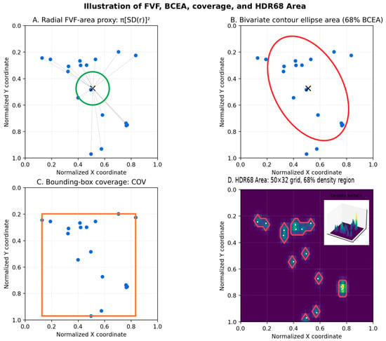
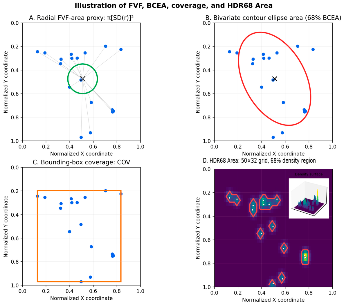
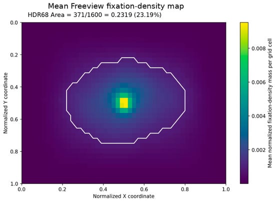
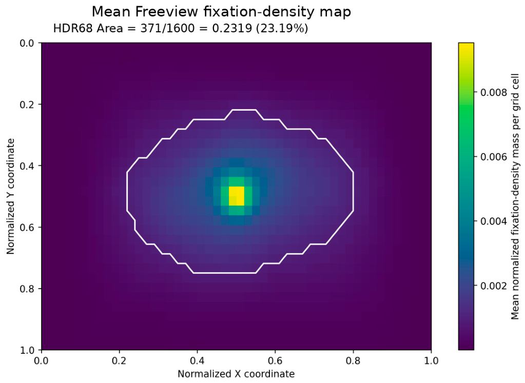
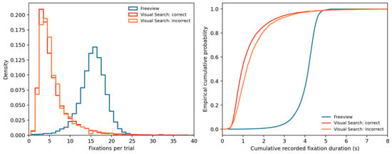
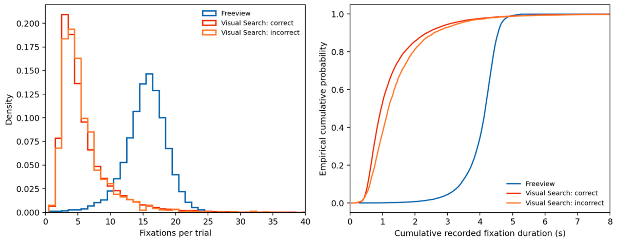
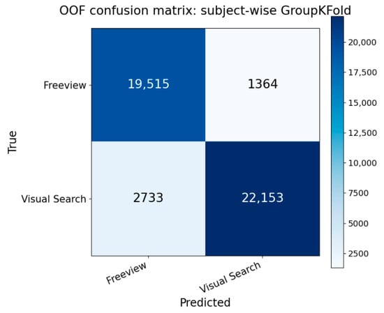
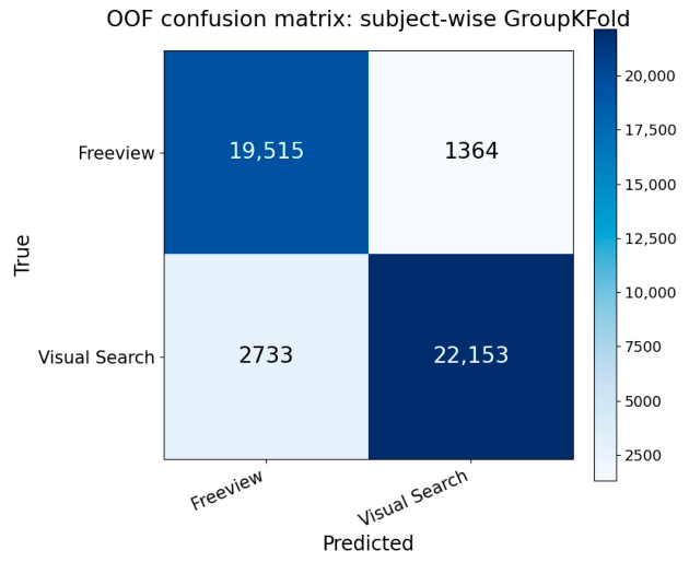
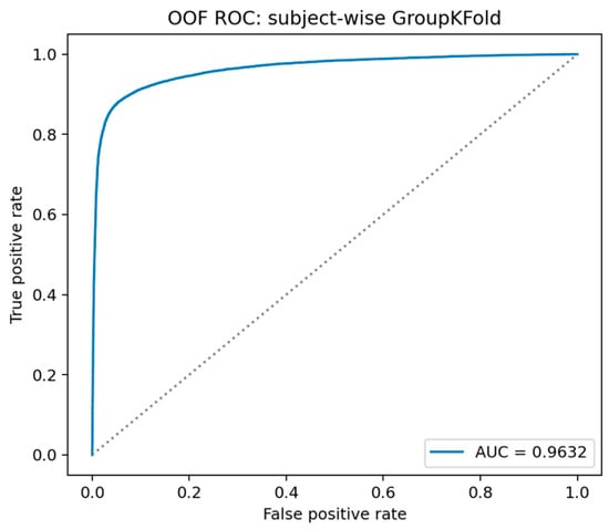

Disclaimer/Publisher’s Note: The statements, opinions and data contained in all publications are solely those of the individual author(s) and contributor(s) and not of MDPI and/or the editor(s). MDPI and/or the editor(s) disclaim responsibility for any injury to people or property resulting from any ideas, methods, instructions or products referred to in the content. |
© 2026 by the authors. Licensee MDPI, Basel, Switzerland. This article is an open access article distributed under the terms and conditions of the Creative Commons Attribution (CC BY) license.