Refining Retinal Vessel Segmentation with Conditional Diffusion Models: A Controlled Evaluation on LU-Net+RA Probability Maps

Abstract

Retinal vessel segmentation remains difficult along thin, low-contrast branches. We evaluate a conditional diffusion refiner for probability maps from a lightweight U-Net with reverse attention (LU-Net+RA). A frozen mask autoencoder produces a spatially downsampled multi-channel grid; a global RGB embedding conditions denoising diffusion implicit model (DDIM) updates, followed by frozen decoding. The refiner adds 527,233 parameters to the 1,946,961-parameter backbone. Matched evaluation on CHASE-DB1, DRIVE and HRF uses five training seeds and five sampling seeds. Refined mean Dice was 0.746, 0.790 and 0.666, against coarse values of 0.811, 0.792 and 0.732. Exploratory paired intervals exclude zero in the negative direction. Conditioning variants changed Dice by less than 0.0002. Deterministic encoded-grid refinement and autoencoder fine-tuning narrowed the gap but exceeded the baseline only on DRIVE; spatial residual refinement changed Dice by −0.0001, +0.0058 and +0.0074. Matched out-of-fold training did not establish absence of input shift. Increasing DDIM updates from 50 to 100 doubled refinement time with negligible observed Dice change. An earlier single-run result was not reproduced. Under this controlled protocol, diffusion refinement did not improve LU-Net+RA.

1. Introduction

Retinal vessel segmentation supports quantitative analysis of vascular morphology in fundus images and may assist research on ocular and systemic disease. Convolutional neural network (CNN)-based methods have become a common approach to this task, including architectures such as U-Net and its variants, volumetric models such as V-Net [1], and context-aware designs such as CE-Net [2]. Despite these advances, several technical challenges remain.

A primary difficulty is that vessel pixels occupy a relatively small part of a fundus image, producing substantial class imbalance. Under this imbalance, standard pixel-wise losses can underemphasise small structures, motivating alternatives such as focal loss [3]. Thin vessels and boundaries may also have low contrast, increasing the risk of missed or over-smoothed predictions. In addition, iterative refinement introduces a practical trade-off between predictive performance and computational cost.

Recent work has addressed some of these issues with lightweight architectures such as LU-Net with reverse attention (LU-Net+RA), which combines depth-wise separable convolutions with an attention mechanism intended to focus computation on missed regions [4]. Because a single feed-forward prediction cannot revise itself, an explicit post-processing model offers a mechanism for correcting missed vessel pixels and uncertain boundaries while retaining the coarse predictor as a fixed first stage. We therefore study segmentation refinement: a conditional diffusion module receives an LU-Net+RA probability map and the corresponding fundus image, then produces a revised vessel-probability map.

This work introduces a conditional diffusion model that operates on an encoded coarse map as a dedicated refinement stage. Denoising diffusion probabilistic models (DDPMs) provide an iterative formulation for generation and restoration [5,6], whereas latent diffusion performs the updates in an autoencoder representation [7]. The representation used here is spatially downsampled but is not compressed in scalar count; we therefore call it a spatially downsampled multi-channel representation rather than a latent or compressed space. We test, on the same test images and with five training seeds per configuration, whether the refiner improves the coarse LU-Net+RA predictions. An earlier single-run experiment with an archived version of the refiner gave higher Dice than published LU-Net+RA results, but its trained checkpoint and complete machine-readable prediction maps are no longer available for re-evaluation. We therefore re-implemented the refiner with a fully documented protocol and saved all test predictions. Under this protocol, the refiner did not improve the coarse predictions. We report this result together with component ablations, deterministic refiners and latency measurements that indicate where the shortfall arises.

• Contributions.

This work makes the following contributions:

• We propose a conditional diffusion module that operates on coarse LU-Net+RA probability maps by applying continuous Gaussian diffusion to the encoded coarse prediction, rather than to an encoded ground-truth target; it combines the encoded mask with a global red–green–blue (RGB) image embedding and returns a refined vessel-probability map through a frozen mask decoder, and we give a layer-level specification of the denoiser.
• We document the component interfaces and parameter budget of the refinement stack, counted with the same convention as the 1,946,961-parameter LU-Net+RA backbone: a 0.121 M-parameter mask autoencoder, a 0.028 M-parameter image encoder, a 0.353 M-parameter diffusion U-Net and a 0.025 M-parameter conditioning network, for 527,233 parameters in total; an earlier subtotal of 502,401 omitted the conditioning network.
• We compare refined and coarse predictions on the same CHASE-DB1, DRIVE and HRF test images with five training seeds, and find that the refiner does not improve mean Dice on any dataset.
• We report component ablations (deterministic refinement, target diffusion, conditioning variants and autoencoder fine-tuning) and a spatial residual refiner; the conditioning choice has negligible effect, and the results point to the frozen, spatially downsampled mask encoding as a plausible contributor to the observed loss.
• We measure complete-pipeline latency and the effect of 50 versus 100 DDIM updates, and present full-image and zoomed qualitative comparisons from the controlled global/frozen reference experiment.

• Overview.

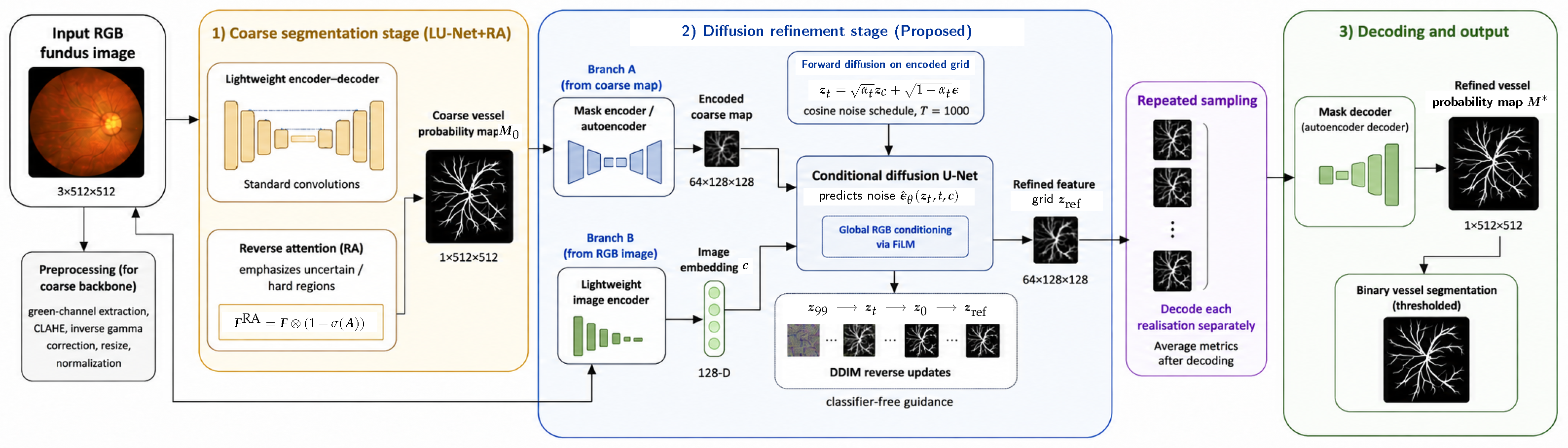
Figure 1 illustrates the overall framework, comparing the conventional single-stage LU-Net+RA pipeline with the proposed two-stage approach, in which a diffusion module refines the initial segmentation through iterative correction of the encoded coarse map.

Figure 1. Workflow of the proposed two-stage framework. The ellipses indicate intermediate DDIM updates omitted from the schematic. The encoded coarse map is ${\mathit{z}}_c$, and ${\mathit{z}}_{\mathrm{ref}}$ denotes the clean endpoint of the reverse updates. Stage 1 applies vessel-enhancement preprocessing and LU-Net with reverse attention to produce the coarse vessel mask ${\mathit{M}}_0$. In Stage 2, the frozen mask encoder maps ${\mathit{M}}_0$ to a spatially downsampled multi-channel grid, which is noised and refined by the conditional diffusion U-Net using deterministic DDIM updates. A separate RGB image encoder supplies the 128-dimensional conditioning vector, which modulates the denoiser through feature-wise linear modulation (FiLM). The frozen mask decoder produces the refined vessel-probability map ${\mathit{M}}^{*}$. When several sampling seeds are evaluated, each realisation is decoded separately and metrics are averaged after decoding.

The remainder of this paper is organised as follows. Section 2 reviews prior work on vessel segmentation and diffusion-based refinement. Section 3 describes the coarse predictor and proposed refinement method. Section 4 presents the experimental protocol, segmentation results, and qualitative analyses. Section 5 and Section 6 discuss the evidence, limitations, and conclusions.

2. Related Work

2.1. Retinal Vessel Segmentation

Early retinal vessel segmentation methods relied on hand-crafted features, such as Gabor filters and matched filtering, combined with thresholding or classical classifiers [8,9]. While effective in controlled settings, these approaches lack robustness to variations in illumination and vessel appearance.

With the advent of deep learning, convolutional neural networks (CNNs), particularly U-Net [10], became the dominant paradigm for biomedical image segmentation, achieving strong performance on benchmark datasets such as DRIVE [11]. Subsequent work has focused on improving architectural design, including nested structures (UNet++ [12]), attention mechanisms [13,14], and recurrent or residual connections [15], as well as incorporating vessel-specific priors such as connectivity constraints and boundary information [16,17,18].

More recently, lightweight architectures such as LU-Net+RA [4] have aimed to balance accuracy and efficiency by leveraging depth-wise separable convolutions and reverse attention. Thin-vessel recovery and structural continuity remain relevant evaluation targets, particularly in low-contrast regions. These targets motivate testing whether a separate refinement strategy changes coarse predictions beneficially under a controlled protocol.

2.2. Diffusion Models

Diffusion models learn to reverse a progressive noise process [5]. DDIM permits deterministic transitions along a reduced timestep sequence [19], while latent diffusion performs these updates in an autoencoder representation [7].

Diffusion models have also been investigated for medical image segmentation. Wolleb et al. [20] generated implicit segmentation ensembles, while SegDiff and MedSegDiff adapted conditional diffusion to general and medical segmentation tasks [21,22]. Pre-segmentation diffusion sampling starts the reverse process from a noised preliminary mask rather than pure Gaussian noise [23], which is conceptually close to the initialisation used here. A broader survey is provided by Kazerouni et al. [24].

Recent work is more directly related to coarse-to-fine refinement. HiDiffSeg combines a coarse vessel estimate, vessel skeleton, and fundus-image guidance in a hierarchical diffusion model for retinal vessel segmentation [25]. RefineCatDiff uses a coarse probability map as prior knowledge in a categorical diffusion process for medical image segmentation [26]. Li et al. [27] instead introduce a plug-and-play diffusion denoising module for end-to-end feature-map refinement. The present method differs in four respects: it applies continuous Gaussian diffusion to the encoded LU-Net+RA probability map; freezes a mask autoencoder during refinement training; conditions the denoiser with a global RGB embedding; and adds 527,233 parameters as a post-processing stage. These distinctions define the architectural contribution, but they do not establish performance superiority because no controlled comparison with these methods is available. We did not reproduce these three methods under our protocol: they diffuse different quantities (skeleton-guided hierarchical maps, categorical labels and intermediate feature maps), so each would need a separate implementation and tuning. Because our refiner does not improve its own coarse input (Section 4.4), we compare it instead with two deterministic learned refiners (Section 4.5 and Section 4.6).

Unlike formulations that diffuse an encoded ground-truth target, the proposed training process adds noise to the encoded coarse mask and uses a decoded Dice term to encourage agreement with the reference mask. This choice makes the method a Dice-regularised denoiser of the coarse prediction rather than a conventional target-diffusion model. Section 4.5 reports a deterministic learned-refiner control and a target-diffusion ablation that isolate the contribution of the diffusion formulation.

2.3. Attention Mechanisms in Medical Imaging

Attention mechanisms are widely used in medical imaging to enhance feature representation by focusing on relevant regions. Channel and spatial attention modules, such as SE-Net [28] and CBAM [29], improve performance by reweighting feature responses. In contrast, reverse attention [4] explicitly emphasises regions that are likely to be misclassified, enabling the model to focus on difficult structures.

3. Methods

3.1. Problem Formulation

Bold italic symbols denote vectors, matrices and tensors; regular-weight italic symbols denote scalars and individual entries. Descriptive subscripts are upright. Thus, $\mathit{M}$ denotes a complete mask, whereas $M_p$ denotes its scalar entry at pixel p.

Retinal vessel segmentation is formulated as a dense prediction task in which each pixel of a fundus image is classified as vessel or background. Let $\mathit{I}\in {\mathbb{R}}^{3\times 512\times 512}$ denote an RGB fundus image, and let ${\mathit{M}}_{\mathrm{gt}}\in {\{0,1\}}^{1\times 512\times 512}$ denote the corresponding ground-truth mask. The objective is to learn a mapping $\mathcal{F}:\mathit{I}\mapsto {\mathit{M}}^{*}$, where ${\mathit{M}}^{*}\in {[0,1]}^{1\times 512\times 512}$ is the predicted vessel-probability map (thresholded to obtain a binary mask during evaluation).

Instead of a single-stage prediction, we adopt a coarse-to-fine framework. A lightweight segmentation model first produces a coarse estimate ${\mathit{M}}_0\in {[0,1]}^{1\times 512\times 512}$, which captures the main vessel structure but may contain discontinuities, missing thin vessels, and blurred boundaries.

To refine this estimate, ${\mathit{M}}_0$ is mapped to a spatially downsampled multi-channel representation ${\mathit{z}}_c=\mathrm{Encode}\left({\mathit{M}}_0\right)$, where $\mathrm{Encode}(·)$ denotes a mask encoder and ${\mathit{z}}_c\in {\mathbb{R}}^{C\times H\times W}$ is a spatially downsampled learned grid. A conditional diffusion model ${\mathrm{Refine}}_{\theta }(·)$ then updates ${\mathit{z}}_c$ iteratively while conditioning on the input image $\mathit{I}$. The refined grid is mapped back to pixel space using a decoder $\mathrm{Decode}(·)$, yielding:

$${\mathit{M}}^{*}=\mathrm{Decode}\left({\mathrm{Refine}}_{\theta }({\mathit{z}}_c,\mathit{I})\right).$$

(1)

This formulation separates coarse prediction from iterative refinement and provides a tunable additional-computation stage.

3.2. Baseline: Lightweight U-Net with Reverse Attention

For coarse segmentation, we use LU-Net+RA [4], a lightweight encoder–decoder; the released one-channel LNet_RA implementation used here employs standard convolutions and reduced channel widths. Its key component is reverse attention (RA), which emphasises uncertain regions. Given a feature map $\mathit{F}$ and attention logits $\mathit{A}$, the RA output is

$${\mathit{F}}^{\mathrm{RA}}=\mathit{F}\otimes \left(1-\sigma \left(\mathit{A}\right)\right),$$

(2)

where $\sigma (·)$ is the sigmoid function and ⊗ denotes element-wise multiplication. Here, $\sigma \left(\mathit{A}\right)$ highlights predicted vessel regions, while its complement focuses the model on hard or misclassified areas. The resulting reverse-attention-modulated features are decoded to produce the coarse prediction ${\mathit{M}}_0$ used by the diffusion refinement stage.

Importantly, this RA mechanism is used only within the LU-Net+RA backbone. The diffusion refiner itself does not receive a separate RA map tensor as an additional input. Instead, the diffusion stage is conditioned on the encoded coarse mask ${\mathit{z}}_c=\mathrm{Encode}\left({\mathit{M}}_0\right)$ and the image embedding $\mathit{c}=\mathrm{ImageEncoder}\left({\mathit{I}}_{\mathrm{RGB}}\right)$. In other words, reverse-attention guidance is implemented implicitly via the RA-enhanced coarse prediction ${\mathit{M}}_0$, rather than as an explicit extra conditioning channel in the diffusion U-Net.

3.3. Proposed Conditional Diffusion Refiner

To refine the coarse segmentation, we operate on a learned multi-channel grid with lower spatial resolution than the input mask. The proposed refinement framework consists of a mask autoencoder, an image encoder for conditioning, and a conditional diffusion model defined in this learned representation space.

Parameters are counted as unique registered weights and biases, including frozen modules and excluding buffers and optimiser states. Under this convention, the released LU-Net+RA has 1,946,961 parameters; its 3028 buffer elements are excluded. An earlier subtotal of 502,401 refinement parameters covered the mask autoencoder, image encoder and diffusion U-Net but omitted the archived implementation’s separate 33,024-parameter conditioning MLP; including it gives 535,425 parameters, 27.50% of the backbone. The executable configuration used in all experiments has a 24,832-parameter time-conditioning MLP instead, giving 527,233 refinement parameters, 27.08% of the backbone (Table 1 and Table 2). These counts describe storage and training budgets; sequential sampling adds inference cost, which Section 4.9 measures.

Table 1. Component interfaces and parameter counts of the refinement module. Counts include frozen components. The executable configuration, used in all experiments, has a time-conditioning MLP; the archived implementation has a separate image-conditioning MLP.

Component	Interface and Role	Executable	Archived
Mask autoencoder	$1\times 512\times 512$ mask $\to 64\times 128\times 128$ grid $\to 1\times 512\times 512$ probability map	121,409	121,409
Image encoder	$3\times 512\times 512$ RGB image → 128-dimensional global embedding	27,712	27,712
Diffusion U-Net with FiLM projections	Noisy grid, timestep and condition → predicted noise	353,280	353,280
Conditioning MLP	Time conditioning (executable) or image conditioning (archived)	24,832	33,024
Full refinement module	Coarse probability map and RGB image → refined vessel-probability map	527,233	535,425

Table 2. Parameter budgets of LU-Net+RA and the complete two-stage systems. The backbone is frozen during refinement training.

Configuration	Backbone	Added Refiner	Complete System	Updated in Refinement
LU-Net+RA	1,946,961	0	1,946,961	0
Executable refiner	1,946,961	527,233	2,474,194	405,824
Archived refiner	1,946,961	535,425	2,482,386	414,016

3.3.1. Mask Autoencoder

We use a lightweight convolutional autoencoder that maps a vessel mask $\mathit{M}\in {\mathbb{R}}^{1\times 512\times 512}$ to a multi-channel grid $\mathit{z}\in {\mathbb{R}}^{64\times 128\times 128}$, corresponding to a $4\times$ reduction along each spatial dimension. The input mask contains $1\times 512\times 512=262,144$ scalar values, whereas the multi-channel grid contains $64\times 128\times 128=1,048,576$ values. It is therefore spatially downsampled but not compressed in scalar count. The architecture is as follows:

• Encoder: Conv($1\to 32$, $3\times 3$, stride 2, padding 1) + ReLU → Conv($32\to 64$, $3\times 3$, stride 2, padding 1) + ReLU → Conv($64\to 64$, $1\times 1$, stride 1).
• Decoder: two $4\times 4$ transposed convolutions ($64\to 64$ and $64\to 32$; stride 2, padding 1), each followed by ReLU, then a $1\times 1$ convolution ($32\to 1$) and sigmoid activation.

Therefore, the spatial path is $512\times 512\to 256\times 256\to 128\times 128$ in the encoder and $128\times 128\to 256\times 256\to 512\times 512$ in the decoder, while the channel progression is $1\to 32\to 64\to 64$ (encoder) and $64\to 64\to 32\to 1$ (decoder). The autoencoder has approximately $0.121$ M trainable parameters in total (about $22,976$ in the encoder and $98,433$ in the decoder).

For an input ground-truth mask ${\mathit{M}}_{\mathrm{gt}}$, the autoencoder reconstruction is

$$\tilde{\mathit{M}}=D_m\left(E_m\left({\mathit{M}}_{\mathrm{gt}}\right)\right).$$

(3)

The reconstruction term is the mean squared error over the $N=512\times 512$ pixels,

$${\mathcal{L}}_{\mathrm{MSE}}(\tilde{\mathit{M}},{\mathit{M}}_{\mathrm{gt}})={\displaystyle \frac{1}{N}}{\displaystyle \sum _{p=1}^N}{\left({\tilde{M}}_p-M_{\mathrm{gt},p}\right)}^2.$$

(4)

For any predicted probability map $\mathit{P}$ and binary target $\mathit{G}$, we use the soft Dice loss

$${\mathcal{L}}_{\mathrm{Dice}}(\mathit{P},\mathit{G})=1-{\displaystyle \frac{2{\sum }_{p=1}^N{P}_p{G}_p}{{\sum }_{p=1}^N{P}_p+{\sum }_{p=1}^N{G}_p}}.$$

(5)

Accordingly, the autoencoder objective is

$${\mathcal{L}}_{\mathrm{AE}}={\mathcal{L}}_{\mathrm{MSE}}(\tilde{\mathit{M}},{\mathit{M}}_{\mathrm{gt}})+{\mathcal{L}}_{\mathrm{Dice}}(\tilde{\mathit{M}},{\mathit{M}}_{\mathrm{gt}}).$$

(6)

All sums are evaluated over the complete resized mask and pooled over the images in a minibatch; the implemented Dice adds $\epsilon ={10}^{-6}$ to its numerator and denominator. For CHASE-DB1 and HRF, the autoencoder is pretrained on ground-truth masks only, without additional mask augmentation, for 50 epochs with AdamW (learning rate ${10}^{-4}$, weight decay ${10}^{-3}$), keeping the checkpoint with the highest validation soft Dice. For DRIVE, it is trained for 200 epochs with AdamW (learning rate ${10}^{-3}$, weight decay ${10}^{-3}$, cosine schedule) on equal batches of in-sample coarse maps and reference masks, reconstructing each input, and the checkpoint with the lowest validation coarse-map reconstruction error is kept. After pretraining, its parameters are frozen and used to encode ${\mathit{M}}_0$. The distribution shift between binary training masks and soft coarse probability maps is analysed as a limitation in the Limitations and Reproducibility subsection.

3.3.2. Image Conditioning

To incorporate global contextual information, the diffusion refinement stage uses a custom lightweight CNN image encoder (not ResNet/MobileNet) fed by the resized and normalised RGB fundus image. Specifically, the encoder receives ${\mathit{I}}_{\mathrm{RGB}}\in {\mathbb{R}}^{3\times 512\times 512}$ and maps it to a compact feature vector $\mathit{c}\in {\mathbb{R}}^{128}$:

$$\mathit{c}=\mathrm{ImageEncoder}\left({\mathit{I}}_{\mathrm{RGB}}\right).$$

(7)

Its layer stack is as follows:

• Conv($3\to 32$, $3\times 3$, stride 2, padding 1) + ReLU;
• Conv($32\to 64$, $3\times 3$, stride 2, padding 1) + ReLU;
• Adaptive average pooling to $1\times 1$;
• Flatten;
• Linear($64\to 128$) to produce the final embedding $\mathit{c}$.

Thus, the feature map is downsampled as $512\times 512\to 256\times 256\to 128\times 128\to 1\times 1$, then projected to a 128-dimensional conditioning vector. This image encoder has approximately $0.028$ M trainable parameters ($27,712$ parameters) and is trained from scratch during diffusion-refiner training (no external pretrained weights are used).

This RGB conditioning branch is separate from the preprocessing used by the coarse LU-Net+RA segmentation backbone. The backbone follows the vessel-enhancement preprocessing pipeline, including green-channel extraction and contrast enhancement, to produce the coarse vessel-probability map ${\mathit{M}}_0$. In contrast, the diffusion image encoder is not given a green-channel-only image or a CLAHE-enhanced single-channel input; it receives the three-channel RGB fundus image after resizing and normalisation. This design allows the refiner to exploit colour and illumination cues while the diffusion process operates on the encoded coarse mask.

3.3.3. Diffusion on the Encoded Grid

The refinement is formulated as a diffusion process in the encoded representation. Starting from the encoded coarse mask ${\mathit{z}}_c=\mathrm{Encode}\left({\mathit{M}}_0\right)$, noise is progressively added according to a cosine schedule [30]:

$$a_t={\displaystyle \frac{{\cos }^2\left(\frac{t/T+0.008}{1.008}·\frac{\pi }{2}\right)}{{\cos }^2\left(\frac{0.008}{1.008}·\frac{\pi }{2}\right)}},$$

(8)

where $t\in \{0,\dots ,T\}$ denotes the diffusion step and $T=1000$. The implementation derives per-step rates ${\beta }_k=\min (1-a_{k+1}/a_k,0.999)$ and stores the cumulative signal-retention products ${\overline{\alpha }}_k={\prod }_{j=0}^k(1-{\beta }_j)$ for the zero-based indices $k=0,\dots ,999$, so the stored ${\overline{\alpha }}_0$ is slightly below one. Training timesteps are sampled uniformly from $\{0,\dots ,999\}$, and inference uses 50 DDIM updates (Section 3.3.6). The forward process generates noisy encoded variables:

$${\mathit{z}}_t=\sqrt{{\overline{\alpha }}_t}{\mathit{z}}_c+\sqrt{1-{\overline{\alpha }}_t}\mathit{ϵ},\mathit{ϵ}\sim \mathcal{N}(0,\mathit{I}),$$

(9)

where $\mathit{ϵ}$ is Gaussian noise. The clean encoder output is denoted by ${\mathit{z}}_c$ to distinguish it from the noisy variable at stored schedule index zero.

A conditional diffusion U-Net is then trained to reverse this process by predicting the noise component ${\widehat{\mathit{ϵ}}}_{\theta }({\mathit{z}}_t,t,\mathit{c})$, conditioned on both the noisy encoded tensor ${\mathit{z}}_t$ and the image embedding $\mathit{c}$.

3.3.4. Conditioning Injection and Denoiser Layers

In the executable configuration, a $64\to 128\to 128$ MLP with SiLU projects the sinusoidal timestep embedding and adds it to the 128-dimensional image embedding $\mathit{c}$. In each residual block of the diffusion U-Net, a $128\to 128$ linear projection of this combined vector supplies 64 scales and 64 shifts for feature-wise linear modulation (FiLM). Each residual block applies GroupNorm with eight groups, SiLU, a convolution, FiLM, a second convolution and SiLU, and then adds the block input; Table 3 lists the layers. This feature-wise conditioning supplies global fundus context throughout denoising without introducing a separate spatial cross-attention map. Reverse attention remains confined to the LU-Net+RA backbone that produces the coarse mask ${\mathit{M}}_0$; no separate RA tensor is injected into the diffusion U-Net. Residual connections are internal to the blocks; there is no additional encoder–decoder concatenation skip. The output predicts noise.

Table 3. Layers of the diffusion U-Net (denoiser) in the executable configuration. The encoded input has 64 channels.

Layer	Channels	Kernel/Stride/Padding	Spatial Size
Input convolution	$64\to 64$	3/1/1	$128\times 128$
Residual FiLM block	$64\to 64$	Two 3/1/ 1 convolutions	$128\times 128$
Down convolution	$64\to 64$	4/2/1	$64\times 64$
Residual FiLM block	$64\to 64$	Two 3/1/1 convolutions	$64\times 64$
Transpose convolution	$64\to 64$	4/2/1	$128\times 128$
Output convolution	$64\to 64$	1/1/0	$128\times 128$

3.3.5. Training Objective

The model is trained to predict the noise added during the forward diffusion process while incorporating segmentation-aware constraints. Let $N_z$ be the number of elements in an encoded tensor. The mean DDPM noise-prediction loss is

$${\mathcal{L}}_{\mathrm{DDPM}}={\mathbb{E}}_{{\mathit{z}}_c,t,\mathit{ϵ}}\left[{\displaystyle \frac{1}{N_z}}{∥{\widehat{\mathit{ϵ}}}_{\theta }({\mathit{z}}_t,t,\mathit{c})-\mathit{ϵ}∥}_2^2\right],$$

(10)

with $\mathit{ϵ}\sim \mathcal{N}(0,\mathit{I})$ denoting Gaussian noise and ${\mathit{z}}_t$ the noisy encoded tensor obtained from ${\mathit{z}}_c$ at timestep t. The noise prediction is then used to estimate the clean encoded tensor corresponding to the sampled timestep:

$${\hat{\mathit{z}}}_c^{\left(t\right)}={\displaystyle \frac{{\mathit{z}}_t-\sqrt{1-{\overline{\alpha }}_t}{\widehat{\mathit{ϵ}}}_{\theta }({\mathit{z}}_t,t,\mathit{c})}{\sqrt{{\overline{\alpha }}_t}}}.$$

(11)

Because the pretrained mask decoder is frozen and includes its output sigmoid, the associated vessel-probability map is

$${\hat{\mathit{M}}}_t=D_m\left({\hat{\mathit{z}}}_c^{\left(t\right)}\right).$$

(12)

The segmentation-aware term is therefore ${\mathcal{L}}_{\mathrm{Dice}}({\hat{\mathit{M}}}_t,{\mathit{M}}_{\mathrm{gt}})$, using the pixel-space definition given above, and the complete diffusion-refiner objective is

$$\mathcal{L}={\mathcal{L}}_{\mathrm{DDPM}}+{\lambda }_{\mathrm{dice}}{\mathcal{L}}_{\mathrm{Dice}}({\hat{\mathit{M}}}_t,{\mathit{M}}_{\mathrm{gt}}).$$

(13)

In the implementation evaluated here, ${\lambda }_{\mathrm{dice}}=0.5$; no separate Sobel edge-loss term is applied. This weight was fixed in advance and not tuned.

This objective is Dice-regularised denoising of the encoded coarse mask. The DDPM term is defined with respect to Gaussian noise added to $E_m\left({\mathit{M}}_0\right)$ and therefore favours recovery of the coarse encoded grid, whereas the decoded Dice term encourages agreement with the ground-truth vessel mask. The method is not formulated as unconditional generation of $E_m\left({\mathit{M}}_{\mathrm{gt}}\right)$. This distinction is important when comparing it with formulations that diffuse the ground-truth target and provide the coarse mask as a separate condition.

The models are trained in two stages. The mask autoencoder is pretrained as described in Section 3.3.1. Its weights are then frozen, and the diffusion refiner is trained for 100 epochs using AdamW at $1\times {10}^{-4}$ with cosine annealing over the full training schedule, weight decay ${10}^{-3}$, batch size four and gradient clipping at one; the predefined final epoch-100 checkpoint is evaluated. No learning-rate warm-up is used: the refiner starts at the stated initial learning rate and follows cosine annealing from the first epoch. During diffusion training, only the image encoder, conditioning multilayer perceptron (MLP), and diffusion U-Net are updated. A classifier-free-guidance conditioning dropout of 10% is applied during training. No additional image or mask augmentation is used. Images and masks are resized to $512\times 512$, and LU-Net+RA probability maps are loaded as the coarse conditions. No explicit field-of-view loss mask or crop is applied during refiner training.

3.3.6. DDIM Sampling

For inference, we employ DDIM sampling [19] to generate a refined encoded representation from the initial code ${\mathit{z}}_c=\mathrm{Encode}\left({\mathit{M}}_0\right)$. Instead of starting from pure noise, the sampling process is initialised from a noisy version of ${\mathit{z}}_c$, preserving an explicit connection to the coarse prediction throughout the refinement trajectory.

The starting timestep $t_s$ controls refinement strength: a larger value adds more noise to the encoded coarse mask and permits a stronger correction, whereas a smaller value preserves more of the LU-Net+RA prediction. Coarse-initialised diffusion uses $t_s=99$. The target-diffusion Gaussian-start ablation instead starts from pure Gaussian noise at index 999, and the deterministic encoded-grid control uses no DDIM sampling. The strength $\rho$ of the earlier single-run experiment was not recorded. The S retained indices are spaced by integer truncation between $t_s$ and zero, and the last update projects from index zero to the clean endpoint, so S counts the denoiser-driven updates (DDIM transitions). At every reverse step, the diffusion U-Net is evaluated with both the image condition and a null condition. Their predictions are combined using classifier-free guidance with scale 1.5, after which the deterministic DDIM update (${\eta }_{\mathrm{DDIM}}=0$) maps the current feature tensor to the next timestep. Because the mask decoder already ends with a sigmoid activation, the procedure in Algorithm 1 does not apply a second sigmoid. Each trained stochastic refiner in the matched repeated-training study is evaluated with five initial-noise seeds; each realisation is decoded separately, and metrics, rather than probability maps, are averaged. The fixed-checkpoint repeated-sampling experiment has a separate protocol (Section 4.8). Although each reverse trajectory is deterministic after its initial noise sample is fixed, the complete procedure remains stochastic with respect to that initial sample.

Algorithm 1: Refinement sampling procedure of the executable configuration

Inputs: coarse mask ${\mathit{M}}_0$; RGB image ${\mathit{I}}_{\mathrm{RGB}}$; encoders $E_m,E_I$; decoder $D_m$; noise network ${\mathit{ϵ}}_{\theta }$; stored schedule ${\left\{{\overline{\alpha }}_k\right\}}_{k=0}^{999}$; start index $t_s=99$; number of DDIM updates S; guidance scale $s=1.5$. Encode ${\mathit{z}}_c=E_m\left({\mathit{M}}_0\right)$ and $\mathit{c}=E_I\left({\mathit{I}}_{\mathrm{RGB}}\right)$; set the null condition ${\mathit{c}}_{Ø}=\mathbf{0}$. Set $t_i=\lfloor t_s(1-i/(S-1))\rfloor$ for $i=0,\dots ,S-1$, so $t_0=t_s$ and $t_{S-1}=0$. Draw $\mathit{ϵ}\sim \mathcal{N}(0,\mathit{I})$ and initialise $\mathit{z}=\sqrt{{\overline{\alpha }}_{t_0}}{\mathit{z}}_c+\sqrt{1-{\overline{\alpha }}_{t_0}}\mathit{ϵ}$. For $i=0,\dots ,S-1$, evaluate ${\mathit{ϵ}}_c={\mathit{ϵ}}_{\theta }(\mathit{z},t_i,\mathit{c})$ and ${\mathit{ϵ}}_u={\mathit{ϵ}}_{\theta }(\mathit{z},t_i,{\mathit{c}}_{Ø})$, and form $\widehat{\mathit{ϵ}}={\mathit{ϵ}}_u+s({\mathit{ϵ}}_c-{\mathit{ϵ}}_u)$. Estimate ${\hat{\mathit{z}}}_c=(\mathit{z}-\sqrt{1-{\overline{\alpha }}_{t_i}}\widehat{\mathit{ϵ}})/\sqrt{{\overline{\alpha }}_{t_i}}$; set $B={\overline{\alpha }}_{t_{i+1}}$ if $i<S-1$ and $B=1$ otherwise; update $\mathit{z}\leftarrow \sqrt{B}{\hat{\mathit{z}}}_c+\sqrt{1-B}\widehat{\mathit{ϵ}}$. Return ${\mathit{M}}^{*}=D_m\left(\mathit{z}\right)$.

4. Experiments and Results

4.1. Datasets and Preprocessing

We evaluate the refiner on three public retinal vessel datasets: the Child Heart and Health Study in England Database 1 (CHASE-DB1) [31], Digital Retinal Images for Vessel Extraction (DRIVE) [11], and High-Resolution Fundus (HRF) [32]. Table 4 reports the released image sizes used by the preprocessing pipeline and the fitting, validation and test partitions used in the reference and matched encoded-grid experiments.

Table 4. Dataset composition and partitions used in the controlled reference and matched encoded-grid experiments. Image sizes refer to the released or cropped images used by the pipeline, not necessarily the acquisition resolution. Partitions use split seed 42 and are fixed across training seeds.

Dataset	Images	Released Image Size	Fitting/Validation/Test	Test n
CHASE-DB1	28	$999\times 960$	16/4/ 8	8
DRIVE	40	$565\times 584$	16/4/20	20
HRF	45	$3504\times 2336$	27/6/12	12

CHASE-DB1 contains images of both eyes from 14 children; its partitions are grouped by subject (8/2/4 subjects), keeping both eyes of each child together, and first-observer annotations are used for all evaluations. DRIVE has an official 20-image training set and 20-image test set; its training pool is split into 16 fitting and four validation images. HRF contains 15 healthy, 15 diabetic-retinopathy, and 15 glaucomatous images; its partitions are stratified by group, with 9/2/4 fitting/validation/test images per group. The HRF field-of-view masks are decoded from Supervisely-format annotation files, whose conversion from the original annotations is not documented.

Two preprocessing streams are used. The LU-Net+RA backbone follows the preprocessing pipeline of Hernandez-Gutierrez et al. [4]: green-channel extraction, contrast-limited adaptive histogram equalisation (CLAHE), inverse gamma correction, resizing to $512\times 512$, and normalisation to $[0,1]$. This stream produces the coarse probability map ${\mathit{M}}_0$. The refiner receives ${\mathit{M}}_0$, while its image encoder receives the corresponding resized and normalised RGB fundus image. RGB images and the preprocessed green channel are resized with bilinear interpolation, and binary annotations and FOV masks with nearest-neighbour interpolation, on a square canvas without preserving the native aspect ratio.

4.2. Training and Implementation Details

Training is sequential. LU-Net+RA is trained first and then frozen. Its stored probability maps condition the refiner, whose training does not update the backbone. The coarse maps used to train the refiner were generated from images that had also been used to fit LU-Net+RA; they are therefore in-sample rather than out-of-fold predictions. Freezing prevents joint adaptation between the stages, but it does not remove the possible train–test shift between in-sample coarse predictions and predictions for unseen images.

LU-Net+RA is trained with Dice loss and AdamW (learning rate ${10}^{-3}$, weight decay ${10}^{-3}$), batch size four, at most 1000 epochs and early stopping with patience 20, keeping the checkpoint with the highest validation mean image Dice; its training applies aligned rotations (0, 15, 30, 45, 90, 100 and 120 degrees) and independent horizontal and vertical flips with probability 0.5. The mask autoencoder and reference refiner are trained as described in Section 3.3; the refiner uses conditioning dropout of 10% and no additional geometric, image, or mask augmentation; no test result is used for checkpoint selection. The reference and matched encoded-grid configurations are trained five times, with seeds 42, 123, 2026, 3000 and 3001 and the same fixed partitions; each seed is a separate training run, and refiner optimisation noise and dropout use the training seed plus 98765, identically across matched variants. Each trained stochastic refiner in these matched repeated-training configurations is evaluated with five initial-noise seeds (42, 123, 2026, 3000 and 3001). The deterministic encoded-grid control is evaluated once per image without sampling (Section 4.5). For these repeated-training configurations, FP32 test predictions, annotations, FOV masks and confusion counts are saved, and their metrics are computed from these outputs. The spatial refiner uses its separate augmentation recipe (Section 4.6). Section 4.8 instead uses one fixed trained model and twenty initial-noise seeds; its archived score and timing records are retained, but complete repeat-level probability arrays were not retained for fresh mask-level verification.

Timing uses one NVIDIA GeForce RTX 4070 Ti SUPER graphics processing unit in evaluation mode (Santa Clara, CA, USA), with gradient computation disabled, FP32 and a batch size of 1; Section 4.8 and Section 4.9 give the measurement protocols.

4.3. Evaluation Protocol and Metrics

Vessel pixels are treated as the positive class. Let TP, TN, FP, and FN denote true-positive, true-negative, false-positive, and false-negative pixel counts, respectively. The metrics appearing in the result tables are

$$\mathrm{Dice}={\displaystyle \frac{2\mathrm{TP}}{2\mathrm{TP}+\mathrm{FP}+\mathrm{FN}}},$$

(14)

$$\mathrm{Accuracy}={\displaystyle \frac{\mathrm{TP}+\mathrm{TN}}{\mathrm{TP}+\mathrm{TN}+\mathrm{FP}+\mathrm{FN}}},$$

(15)

$$\mathrm{Sensitivity}={\displaystyle \frac{\mathrm{TP}}{\mathrm{TP}+\mathrm{FN}}},$$

(16)

$$\mathrm{Specificity}={\displaystyle \frac{\mathrm{TN}}{\mathrm{TN}+\mathrm{FP}}}.$$

(17)

Predictions are binarised at probability 0.5. Metrics are computed per image, over the whole image for CHASE-DB1 and within the field-of-view (FOV) mask for DRIVE and HRF, and then averaged over images rather than pooled over pixels. Training losses, by contrast, were evaluated over the full resized canvas, with pixels outside the retinal field represented as background.

For stochastic configurations in the matched repeated-training studies, we average the five sampling realisations within each image and training seed, then average the test images within each seed. Deterministic refiners are evaluated once per image without sampling; the fixed-checkpoint study follows the separate protocol in Section 4.8. For the matched repeated-training studies, tables report the mean and sample SD across the five seed means; sampling draws do not create additional patients or training runs. Paired comparisons use the five matched seed means, with two-sided paired t tests and exact Wilcoxon signed-rank tests and Holm correction within each stated family. With five pairs, the smallest attainable two-sided exact signed-rank probability is 0.0625. Percentile intervals come from a crossed bootstrap with 50,000 draws that jointly resamples training seeds and test units, keeping both eyes of each CHASE-DB1 subject together and resampling HRF images within pathology groups.

4.4. Quantitative Segmentation Results

Table 5 compares the coarse LU-Net+RA predictions with the diffusion refiner (global FiLM conditioning, frozen mask autoencoder, 50 updates) on the same test images: eight CHASE-DB1 images from four subjects, twenty DRIVE images and twelve HRF images. For each training seed, both arms use the same LU-Net+RA checkpoint, annotations, FOV masks, threshold and metric code. Refinement lowered mean Dice on all three datasets, by 0.064 on CHASE-DB1, 0.002 on DRIVE and 0.066 on HRF, so the refiner did not improve its coarse input under this protocol.

Table 5. Paired coarse LU-Net+RA and global/frozen diffusion-refiner Dice at 50 DDIM updates on the same test images. Means and sample SDs are across five training-seed means after averaging five sampling realisations within each image and run. Differences are refiner minus coarse. The 95% intervals are exploratory paired crossed-bootstrap percentile intervals, not simultaneous confidence intervals.

Dataset	Coarse Mean ± SD	Refiner Mean ± SD	Difference
CHASE-DB1	$0.810514\pm 0.001806$	$0.746146\pm 0.002622$	$-0.064368245$
DRIVE	$0.791814\pm 0.007557$	$0.789757\pm 0.008286$	$-0.002057107$
HRF	$0.732121\pm 0.003490$	$0.665726\pm 0.006320$	$-0.066395394$
Dataset	Paired crossed-bootstrap 95% interval
CHASE-DB1	$[-0.078706654,-0.050060076]$
DRIVE	$[-0.003024955,-0.001308524]$
HRF	$[-0.074121150,-0.058866677]$

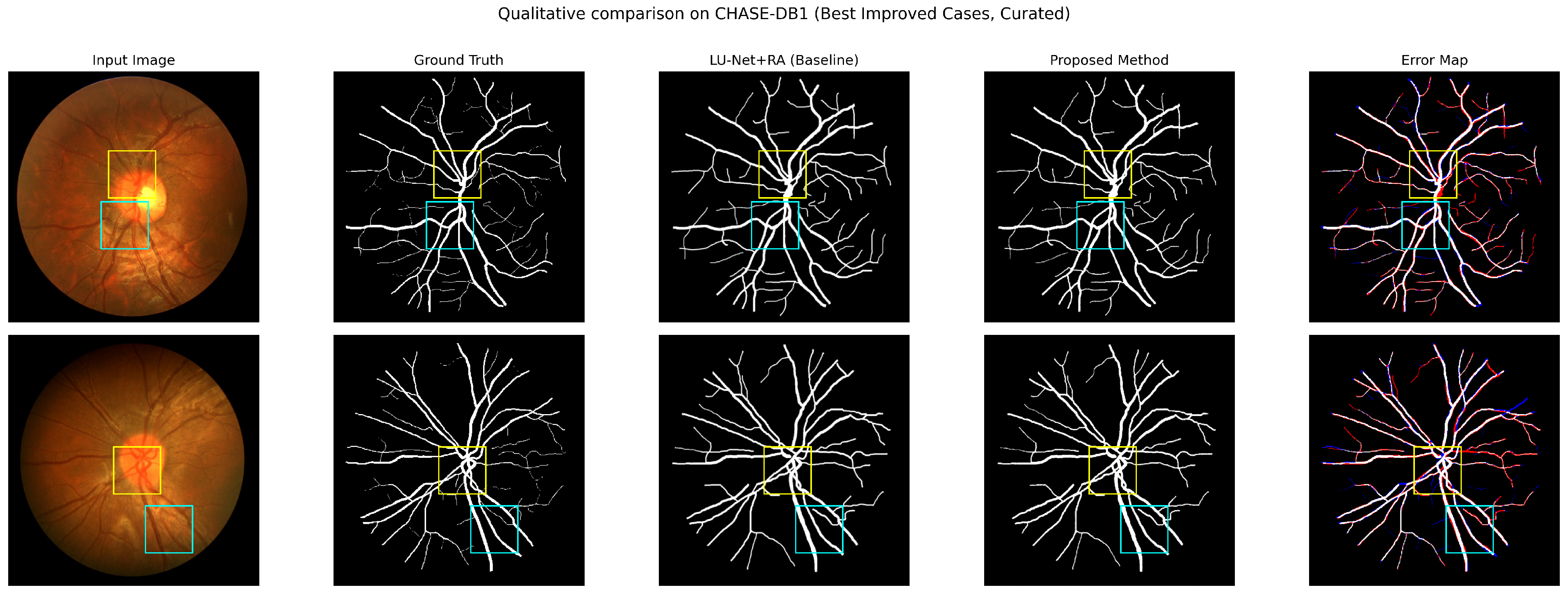
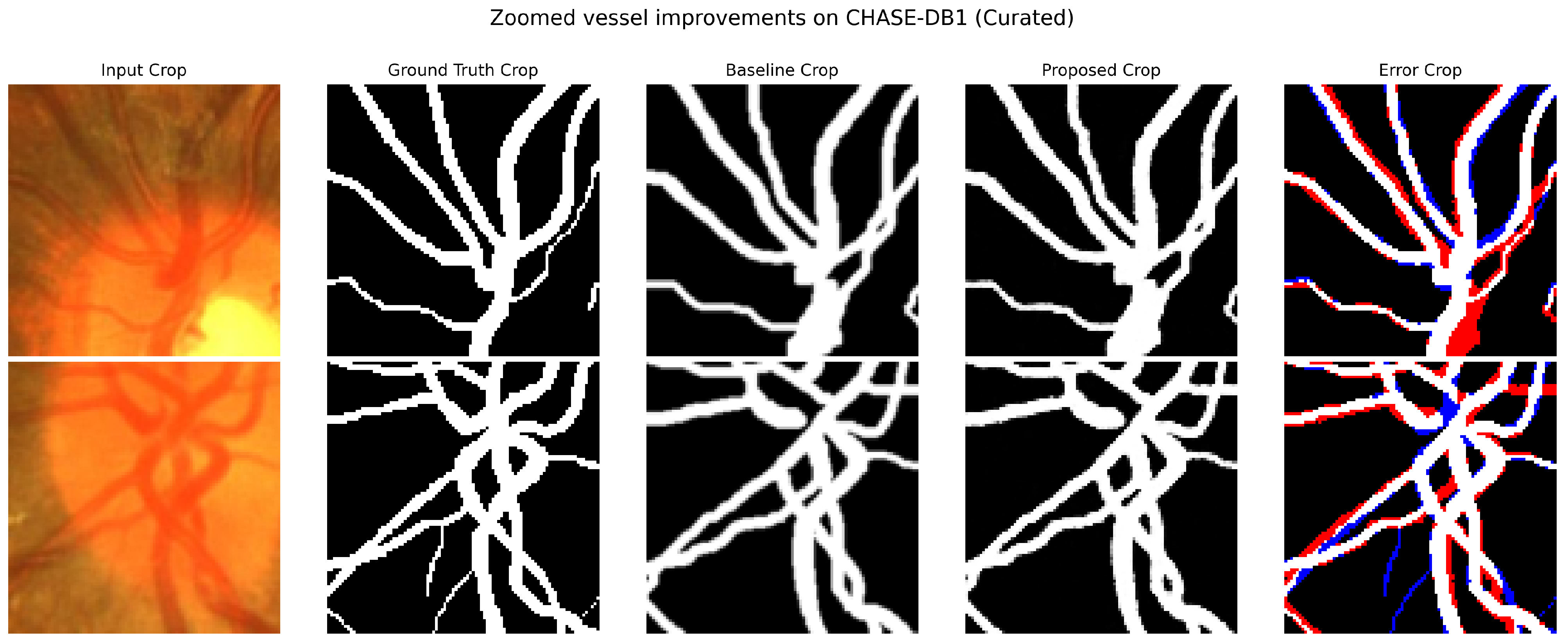
An earlier single-run experiment with an archived version of this refiner reported Dice of 0.835 on CHASE-DB1, 0.835 on DRIVE and 0.793 on HRF at 50 updates, with 20-update values of 0.825, 0.795 and 0.762 and CHASE-DB1 values from 0.814 at 10 updates to 0.836 at 100 updates. The trained checkpoint and complete machine-readable per-image prediction maps of that run are no longer available for re-evaluation. Figure 2 and Figure 3 instead show selected predictions from the controlled global/frozen reference experiment reported in Table 5; they do not originate from that earlier single-run experiment. Its refinement strength, split identities and several training settings were not recorded. The re-implementation documented in Section 3, Section 4.1, Section 4.2 and Section 4.3, trained with five seeds, did not reproduce these scores (Table 5). We therefore no longer report them as results.

Figure 2. Selected CHASE-DB1 examples from the controlled global/frozen reference experiment reported in Table 5, showing the input image, first-observer reference mask, LU-Net+RA coarse prediction, diffusion-refined prediction, and error map for the refined prediction. White, red, blue, and black denote true-positive, false-positive, false-negative, and true-negative pixels, respectively. The coloured rectangles mark the regions enlarged in Figure 3. The examples were selected for visible refinement effects and are illustrative rather than representative.

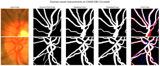
Figure 3. Enlarged regions from selected CHASE-DB1 cases from the controlled global/frozen reference experiment reported in Table 5. Columns show the input crop, first-observer reference mask, LU-Net+RA coarse prediction, diffusion-refined prediction, and refined-prediction error map. White, red, blue, and black denote true-positive, false-positive, false-negative, and true-negative pixels, respectively.

4.4.1. Paired Per-Image Analysis and Uncertainty

Table 6, Table 7 and Table 8 report the per-image results for CHASE-DB1, DRIVE and HRF, respectively.

Table 6. CHASE-DB1 per-image Dice for the Table 5 global/frozen comparison. Each entry averages five training seeds and five sampling realisations. Differences use unrounded paired values and are refined minus coarse. These are per-image means, not independent training replicates.

Image	Coarse Dice	Refined Dice	Difference
Image_02L	0.818734630	0.771136464	$-0.047598166$
Image_02R	0.812283518	0.751455743	$-0.060827775$
Image_05L	0.838999001	0.797081068	$-0.041917933$
Image_05R	0.844530892	0.792050546	$-0.052480346$
Image_09L	0.805841453	0.731423930	$-0.074417523$
Image_09R	0.796916619	0.714857283	$-0.082059336$
Image_13L	0.791873375	0.720846888	$-0.071026487$
Image_13R	0.774932693	0.690314297	$-0.084618395$

Table 7. DRIVE per-image Dice for the Table 5 global/frozen comparison. Each entry averages five training seeds and five sampling realisations. Differences use unrounded paired values and are refined minus coarse. These are per-image means, not independent training replicates.

Image	Coarse Dice	Refined Dice	Difference
01_test	0.797339317	0.794007225	$-0.003332091$
02_test	0.827097574	0.825196260	$-0.001901314$
03_test	0.787253664	0.786541740	$-0.000711924$
04_test	0.804377016	0.803009682	$-0.001367334$
05_test	0.796903799	0.795544806	$-0.001358993$
06_test	0.785758622	0.784951564	$-0.000807059$
07_test	0.800206530	0.798486843	$-0.001719688$
08_test	0.780960260	0.780790909	$-0.000169351$
09_test	0.783184112	0.781780944	$-0.001403168$
10_test	0.785465793	0.783200607	$-0.002265187$
11_test	0.773603814	0.770267795	$-0.003336018$
12_test	0.796731264	0.794527796	$-0.002203469$
13_test	0.793268994	0.791305020	$-0.001963973$
14_test	0.789992603	0.787225844	$-0.002766760$
15_test	0.763721378	0.760549461	$-0.003171917$
16_test	0.808823898	0.806945119	$-0.001878779$
17_test	0.789437261	0.788254205	$-0.001183056$
18_test	0.786173247	0.783883103	$-0.002290144$
19_test	0.802160850	0.796962869	$-0.005197981$
20_test	0.783827712	0.781713769	$-0.002113943$

Table 8. HRF per-image Dice for the Table 5 global/frozen comparison. Each entry averages five training seeds and five sampling realisations. Differences use unrounded paired values and are refined minus coarse. These are per-image means, not independent training replicates.

Image	Coarse Dice	Refined Dice	Difference
01_g	0.710632836	0.652227842	$-0.058404994$
02_h	0.798816139	0.732067972	$-0.066748166$
04_g	0.741554084	0.679006689	$-0.062547395$
07_dr	0.733975667	0.665890830	$-0.068084837$
09_h	0.750261145	0.696942602	$-0.053318542$
10_dr	0.729617456	0.653905035	$-0.075712421$
12_dr	0.697127260	0.636196628	$-0.060930632$
13_g	0.703959510	0.629480025	$-0.074479486$
13_h	0.775788553	0.708332717	$-0.067455836$
14_g	0.701151591	0.632459952	$-0.068691639$
14_h	0.762417806	0.686256277	$-0.076161529$
15_dr	0.680150127	0.615940874	$-0.064209253$

The comparison uses only the global/frozen reference records underlying Table 5: 1000 image–training-seed–sampling-seed records at 50 updates, comprising eight CHASE-DB1, twenty DRIVE and twelve HRF images, five training seeds and five sampling seeds. Both arms use the same cases, coarse checkpoints and evaluation protocol; scores from other refiner variants are excluded. Sampling realisations are averaged within each image and training seed. Per-image entries then average the five training-seed means, while dataset means and sample SDs summarise five run means on the fixed test set. The coarse prediction is repeated across sampling labels and is not counted as an additional independent observation.

For each dataset, an exploratory paired crossed bootstrap uses 50,000 replicates and random seed 20261017. Training seeds and test units are sampled independently with replacement, retaining matched coarse and refined observations. Both CHASE-DB1 eyes remain together within each of four subjects; DRIVE uses image resampling; HRF resamples images within healthy, diabetic-retinopathy and glaucoma strata. Sampling realisations are averaged before resampling. The 2.5th and 97.5th percentiles form the 95% interval. All three intervals for refiner-minus-coarse Dice lie below zero, describing lower mean Dice in this tested configuration. Only four CHASE subjects and five training pairs are available, patient independence is unverified for DRIVE and HRF, and these intervals are exploratory rather than confirmatory or simultaneous. These exploratory intervals are not used as confirmatory hypothesis tests.

4.4.2. Matched Out-of-Fold Coarse-Map Training

The separate matched OOF experiment uses four subject-grouped CHASE-DB1 folds, four DRIVE image folds and three pathology-stratified HRF folds, with fold membership fixed using seed 20261009 across the five training seeds. Each fold predictor is fitted without its held-out images and selected using the separate original validation partition. Held-out fold images and test images are not used for checkpoint selection. Both eyes of each CHASE subject remain together. The experiment comprises 55 fold-baseline fits and 15 OOF-refiner fits. The in-sample arm is the global/frozen reference in Table 5. Both arms share the coarse predictor for the fixed test images, frozen initial mask autoencoder, refiner initialisation, optimisation settings and matched sampling seeds.

Table 9 reports the matched OOF comparison. The matched OOF evaluation averages the sampling realisations before comparison. Five sampling realisations were averaged within each image and training seed, yielding 200 paired image–training-seed records. OOF crossed-bootstrap intervals use 50,000 replicates and seed 20261015, retaining both eyes within CHASE subjects and HRF pathology strata. The OOF-minus-in-sample tests use five matched training-seed means, with Holm correction across the three datasets separately for paired t and exact signed-rank tests. These intervals describe the OOF-minus-in-sample contrast; they are distinct from the coarse-versus-refiner intervals in Table 5.

Table 9. Matched OOF versus in-sample refinement at 50 DDIM updates. The in-sample means and SDs match the global/frozen reference in Table 5. Differences are OOF minus in-sample. Intervals are exploratory crossed-bootstrap intervals; probabilities are Holm-corrected paired training-seed tests, with correction across three datasets separately for each test family.

Dataset	In-sample mean ± SD	OOF mean ± SD	Difference
CHASE-DB1	$0.746145777\pm 0.002622483$	$0.745915967\pm 0.002732575$	$-0.000229810$
DRIVE	$0.789757278\pm 0.008286356$	$0.789614005\pm 0.008314270$	$-0.000143273$
HRF	$0.665725620\pm 0.006319839$	$0.665522152\pm 0.006144710$	$-0.000203468$
Dataset	95% interval	Holm $p_t$	Holm $p_W$
CHASE-DB1	$[-0.000524367,-0.000031774]$	0.283856	0.187500
DRIVE	$[-0.000286638,-0.000032637]$	0.283856	0.250000
HRF	$[-0.000681909,0.000232154]$	0.455162	0.437500

OOF mean Dice is slightly lower on all three datasets. None of the corrected training-seed tests reaches 0.05. The bootstrap intervals exclude zero for CHASE-DB1 and DRIVE but include zero for HRF; these crossed intervals and fixed-test training-seed tests address different uncertainty structures. Nonsignificance does not establish equivalence or absence of train–test shift. Fold predictors fit fewer examples, and the shared frozen DRIVE autoencoder retains in-sample coarse-map pretraining. Small fixed test cohorts and unverified DRIVE/HRF patient independence constrain interpretation.

4.5. Component Ablations

We trained seven refiner configurations with five seeds on each dataset (105 refiners). Within each dataset and training seed, all variants share the partition, the frozen LU-Net+RA checkpoint, the initial mask-autoencoder checkpoint and, where applicable, the initial denoiser weights. Training follows Section 4.2, with no refiner augmentation and the predefined epoch-100 checkpoint. Stochastic variants are evaluated with 50 updates and five matched sampling seeds; the deterministic refiner is evaluated once per image. All 7200 evaluation records were checked against the saved predictions, annotations, FOV masks and confusion counts.

The reference is the refiner of Section 4.4. The deterministic control predicts a residual on the same encoded grid with a fixed zero time input and the decoded Dice loss, without Gaussian noise or DDIM sampling. Target diffusion encodes the training reference mask instead of the coarse map; the same checkpoint is evaluated from the noised coarse map and from pure Gaussian noise, so the second mode also changes the inference start. The remaining variants remove image conditioning, replace the global vector with spatial RGB features and spatial FiLM, replace FiLM with additive injection, or fine-tune the mask encoder and decoder jointly. The reference updates 405,824 parameters, the no-image variant 378,112 and joint fine-tuning 527,233, including 121,409 autoencoder parameters. Global and spatial conditioning have equal parameter counts but different activation costs; the additive variant combines the two FiLM branches as $(g+b)/\sqrt{2}$, which does not preserve effective capacity.

All diffusion variants with the frozen autoencoder remain below the coarse baseline on every dataset (Table 10). Changing the conditioning altered mean Dice by less than 0.0002 relative to the reference, and no conditioning comparison had a Holm-adjusted paired t probability below 0.05. Target diffusion from the coarse start gave similar mean Dice to the reference, whereas a pure Gaussian start failed (Dice 0.03–0.06). The deterministic encoded-grid refiner exceeded the diffusion reference by 0.033, 0.005 and 0.063 on CHASE-DB1, DRIVE and HRF, and joint autoencoder fine-tuning by 0.029, 0.002 and 0.045; both exceeded the coarse baseline only on DRIVE, by 0.0034 and 0.0003. The diffusion formulation therefore offers no advantage over deterministic refinement in this configuration. Paired tests use separate Holm corrections for t and exact signed-rank probabilities over 24 comparisons (seven variants against the reference on each dataset, plus Gaussian versus coarse start for target diffusion); every adjusted signed-rank probability is 1, reflecting the resolution of five pairs.

Table 10. Component ablations: stochastic modes use 50 DDIM updates; the deterministic control uses no DDIM and is evaluated once per image. Entries are mean Dice ± sample SD across five training-seed means, after averaging sampling realisations and test images. All rows share the coarse predictions in the first row.

Configuration	CHASE-DB1	DRIVE	HRF
Coarse LU-Net+RA	$0.810514\pm 0.001806$	$0.791814\pm 0.007557$	$0.732121\pm 0.003490$
Diffusion reference (global FiLM, frozen autoencoder)	$0.746146\pm 0.002622$	$0.789757\pm 0.008286$	$0.665726\pm 0.006320$
Deterministic encoded-grid refiner	$0.779489\pm 0.002450$	$0.795250\pm 0.005437$	$0.728443\pm 0.007471$
Target diffusion, coarse start	$0.747376\pm 0.002848$	$0.789505\pm 0.008478$	$0.663491\pm 0.006222$
Target diffusion, Gaussian start	$0.044834\pm 0.022540$	$0.026778\pm 0.004146$	$0.055330\pm 0.013528$
No image conditioning	$0.746151\pm 0.002620$	$0.789740\pm 0.008297$	$0.665773\pm 0.006406$
Spatial FiLM conditioning	$0.746310\pm 0.002688$	$0.789758\pm 0.008263$	$0.665823\pm 0.006291$
Global additive conditioning	$0.746118\pm 0.002605$	$0.789761\pm 0.008264$	$0.665869\pm 0.006258$
Joint autoencoder fine-tuning	$0.775113\pm 0.004078$	$0.792112\pm 0.005222$	$0.710923\pm 0.009885$

4.6. Spatial Residual Refiner

To test refinement without the encoded grid, we trained a deterministic spatial residual U-Net that receives the RGB image and the coarse probability map as four input channels. It has encoder widths 16, 32, 64 and 128, three skip-connected decoder blocks, bilinear upsampling, GroupNorm and SiLU, and 488,145 parameters. A zero-initialised output layer predicts an additive correction to the coarse logits. The loss weights binary cross-entropy and soft Dice equally. Training used AdamW at $3\times {10}^{-4}$ with weight decay ${10}^{-4}$, cosine scheduling over at most 120 epochs, batch size four, gradient clipping at one, and aligned flips and right-angle rotations of the image, coarse map and annotation; unlike the encoded-grid refiners, this model therefore uses augmentation. The checkpoint was selected by validation mean Dice with patience 25, including the initial zero-residual model, which was selected in two CHASE-DB1 runs and in no DRIVE or HRF run. Five refiners were trained per dataset with the five training seeds and their per-seed coarse predictors, giving 200 paired image–seed records that were checked against the saved predictions.

The spatial refiner changed CHASE-DB1 Dice negligibly and raised DRIVE and HRF Dice by 0.0058 and 0.0074 (Table 11). Both of these intervals exclude zero, but after Holm correction only the HRF paired t probability is below 0.05 and no signed-rank probability is; unadjusted probabilities were 0.2199, 0.0301 and 0.0133 for the t test and 0.25, 0.0625 and 0.0625 for the signed-rank test. Because this refiner differs from the encoded-grid refiners in architecture, input and augmentation, the comparison does not isolate a single factor; it shows that refinement in image space did not lose accuracy where the encoded-grid refiners did.

Table 11. Spatial residual refiner versus coarse LU-Net+RA on the same test images. Entries are mean ± sample SD across five training-seed means. Difference is refined minus coarse; intervals are crossed-bootstrap 95% intervals (50,000 draws). Probabilities are Holm-adjusted across the three datasets, separately for paired t ($p_t$) and exact signed-rank ($p_W$) tests.

Dataset	Coarse	Spatial Refiner	Difference	95% Interval	Holm ${\mathit{p}}_{\mathit{t}}$	Holm ${\mathit{p}}_{\mathit{W}}$
CHASE-DB1	$0.810514\pm 0.001806$	$0.810393\pm 0.001847$	$-0.000121$	$[-0.000343,+0.000011]$	0.2199	0.2500
DRIVE	$0.791814\pm 0.007557$	$0.797647\pm 0.004597$	$+0.005833$	$[+0.001982,+0.010681]$	0.0601	0.1875
HRF	$0.732121\pm 0.003490$	$0.739538\pm 0.001955$	$+0.007417$	$[+0.004093,+0.011327]$	0.0400	0.1875

4.7. Published Literature Context

Table 12 separately reports the baseline U-Net and selected lightweight U-Net with reverse attention results from Table 8 of Hernandez-Gutierrez et al. [4]. The selected LU-Net+RA row uses AdamW, Dice loss without binary cross-entropy loss, and reverse attention on each dataset. This single, explicit source avoids mixing values from the abstract, dataset-comparison tables, discussion, and conclusion of that article, which report internally different CHASE-DB1 and HRF values.

Table 12. Published contextual results from Table 8 of Hernandez-Gutierrez et al. [4]. These values were obtained under that study’s partitioning, validation, preprocessing, and metric procedures and are not paired before-refinement measurements for the test images of Table 5.

Dataset	Published Configuration	Dice	Accuracy	Sensitivity	Specificity
CHASE-DB1	Baseline U-Net	0.7830	0.9725	0.7702	0.9864
	LU-Net+RA (selected Table 8 row)	0.7946	0.9739	0.7795	0.9873
DRIVE	Baseline U-Net	0.7373	0.8931	0.8687	0.9515
	LU-Net+RA (selected Table 8 row)	0.7871	0.9113	0.7421	0.9837
HRF	Baseline U-Net	0.6417	0.8710	0.8559	0.9531
	LU-Net+RA (selected Table 8 row)	0.7756	0.8474	0.7794	0.9793

Our coarse LU-Net+RA predictions give Dice of 0.811, 0.792 and 0.732 on CHASE-DB1, DRIVE and HRF, against published values of 0.7946, 0.7871 and 0.7756. Because the studies use non-identical cases and evaluation pipelines, these numerical differences provide literature context only. The effect of the refiner is measured instead by the paired comparison in Table 5.

4.8. DDIM Transition-Count Analysis

To measure the effect of the update count without training variation, we refined the eight CHASE-DB1 test images with one trained refiner of the reference configuration, using 50 and 100 updates from the same 20 initial-noise tensors, start index 99 and guidance 1.5. Predictions were evaluated against first-observer annotations on the whole $512\times 512$ image at threshold 0.5. Mean Dice was 0.74547638 with 50 updates and 0.74547697 with 100. The mean paired difference was $5.93\times {10}^{-7}$, with a bootstrap 95% interval of $[-9.42\times {10}^{-7},2.03\times {10}^{-6}]$ from 10,000 replicates that resample subjects (with both eyes together) and noise seeds; the SD of the 20 seed-level mean differences was $2.23\times {10}^{-6}$. Mean refinement time rose from 116.98 to 229.64 ms. Timing was CUDA-synchronised and used FP32, batch size one, two warm-up runs per image and setting and alternating measurement order; it covered mask encoding, image conditioning, DDIM sampling and decoding, but not the backbone, transfers or scoring. Doubling the update count therefore doubled refinement time with negligible observed Dice change. This experiment uses one trained model, and its 20 noise seeds are not independent training runs. The interval includes zero, so no reliable Dice benefit from 100 updates is demonstrated; this does not establish equivalence. Update counts below 50 were not evaluated in this protocol.

4.9. Complete-Pipeline Latency

The complete-pipeline benchmark used the retained CHASE-DB1 checkpoints of the reference configuration, FP32, batch size one and the same GPU at 50 DDIM updates. Each of eight test images received five warm-up runs and ten timed repetitions per timing mode in rotated order (80 measurements per mode), with CUDA synchronisation around each call. The complete model was timed directly, not by summing stages. The decoded-RGB-to-mask mode starts from an RGB image already decoded in CPU memory and includes preprocessing, host–device transfers and thresholding, but excludes disk access, image decoding, checkpoint loading and output saving.

The complete model takes about 26 times as long per image as LU-Net+RA alone (Table 13). The separately timed backbone and refinement means sum to 122.46 ms, whereas the directly measured complete model takes 119.02 ms; independently timed calls need not add exactly. In a separate session using CUDA events on GPU-resident inputs, mean stream time was 4.30 ms for LU-Net+RA, 108.30 ms for refinement and 112.02 ms for the complete model. The 116.98-ms refinement time in Section 4.8 comes from another session with two warm-ups.

Table 13. Measured latency at 50 DDIM updates, in milliseconds. Serial rate is $1000/\overline{T}$ images/s. P95 is the empirical 95th percentile, not a confidence interval.

Timing Scope	Mean	SD	Median	P95	Serial Rate
LU-Net+RA only	4.51	0.71	4.23	6.13	221.78
Refinement only	117.95	17.00	112.01	155.30	8.48
Complete model	119.02	12.55	113.86	142.09	8.40
Decoded RGB to CPU binary mask	140.50	15.90	132.67	177.03	7.12

4.10. Qualitative Results

Figure 2 and Figure 3 show selected CHASE-DB1 examples for which visible differences occur between the LU-Net+RA coarse prediction and the diffusion-refined prediction. The panels include the input, first-observer reference, coarse mask, refined mask, and the refined-prediction error map. These examples are selected predictions from the same controlled global/frozen reference experiment reported in Table 5 (Section 4.4). They do not come from the earlier single-run experiment, whose checkpoint and complete prediction maps are unavailable. They illustrate individual cases and do not represent the average refinement effect.

The examples were intentionally selected for visible refinement effects. No inference about average thin-vessel recovery, topology, connectivity, or boundary quality is drawn from these panels; those claims require random or median-case sampling and dedicated centreline, connectivity, or boundary metrics.

5. Discussion

The proposed refiner is most closely related to coarse-to-fine diffusion systems rather than to generic post-processing. HiDiffSeg uses hierarchical vessel and skeleton guidance for retinal segmentation [25]; RefineCatDiff incorporates a coarse probability map as prior knowledge in categorical diffusion [26]; and the diffusion feature-map denoising module of Li et al. [27] is trained end-to-end within existing segmenters. The present design instead performs continuous Gaussian diffusion on an encoded LU-Net+RA probability map, freezes the mask autoencoder, and uses a global RGB condition. These differences motivate the method, but a controlled benchmark is required before claiming an advantage over the related alternatives.

Under matched partitions, preprocessing, annotations, thresholds and test images, the conditional diffusion refiner lowered mean Dice relative to its own coarse input by 0.064 on CHASE-DB1, 0.002 on DRIVE and 0.066 on HRF (Table 5). The higher scores of the earlier single-run experiment were not reproduced, and without its checkpoint we cannot determine which configuration differences produced them.

The ablations indicate where the loss arises. Removing the image condition, replacing the global vector with spatial FiLM or using additive injection changed Dice by less than 0.0002, so the global 128-dimensional condition is not the limiting factor in this configuration. Diffusing the encoded reference mask instead of the coarse map gave similar mean Dice from a coarse start and failed from a Gaussian start. A deterministic refiner on the same encoded grid, or joint fine-tuning of the autoencoder, recovered part of the loss, and a spatial residual refiner that bypasses the encoded grid did not lose accuracy and gave small gains on DRIVE and HRF. These patterns are consistent with the frozen, spatially downsampled mask autoencoder limiting the attainable Dice, and show no benefit of the diffusion formulation over deterministic refinement here. We did not measure the reconstruction ceiling of the autoencoder directly, and the spatial refiner also differs in input and augmentation, so this interpretation remains to be tested.

Refinement adds 27% more parameters and raises per-image latency from 4.5 ms for LU-Net+RA to 119 ms for the complete model, and doubling the number of updates doubles refinement time with negligible observed Dice change. Higher Dice alone would not establish better thin-vessel recovery or connectivity, which require topology-aware metrics that we did not evaluate.

Limitations and Reproducibility

The test sets are small: eight CHASE-DB1 images from four subjects, twenty DRIVE images and twelve HRF images, and patient independence is not documented for DRIVE and HRF. Five training seeds give limited statistical resolution; the smallest two-sided exact signed-rank probability is 0.0625, and crossed-bootstrap intervals may under-cover with so few clusters. Holm corrections control each stated family, not all comparisons in the paper. Latency was measured on one GPU. The earlier single-run result could not be re-evaluated because its trained checkpoint and complete machine-readable prediction maps are unavailable. This limitation concerns that earlier run; Figure 2 and Figure 3 show selected cases from the controlled global/frozen reference experiment, not the earlier run.

The reference refiner is trained on in-sample backbone predictions; Section 4.4.2 reports a separate matched OOF comparison. Neither its nonsignificant paired tests nor its exploratory intervals establish equivalence or rule out train–test input shift. Its fold predictors fit fewer images, and the shared frozen DRIVE autoencoder retains in-sample coarse-map pretraining. In addition, its mask autoencoder is pretrained on binary annotations (for CHASE-DB1 and HRF) but later encodes soft probability maps. Both choices can create a train–test input shift. The global 128-dimensional image vector also discards spatial conditioning information, although replacing it with spatial conditioning had negligible effect (Section 4.5). Finally, the $64\times 128\times 128$ encoded grid is spatially coarser than the input mask but contains more scalar values, so the method should not be described as a compressed latent bottleneck.

We did not reproduce HiDiffSeg, RefineCatDiff or the module of Li et al. under our protocol, and we did not run measured ablations of the Dice-loss weight or of refiner augmentation. The qualitative cases were selected for visible effects, and no centreline, connectivity, boundary, or calibration metric was computed; we removed the earlier qualitative sampling-variance figure because its sample count and display scale could not be documented, and the manuscript makes no calibration claim. Future experiments should extend the matched OOF evaluation, use topology-aware metrics, unbiased qualitative sampling and controlled comparisons with recent coarse-to-fine diffusion refiners, and should test refinement without a frozen, spatially downsampled mask encoding.

6. Conclusions

We specified and evaluated a conditional diffusion refiner for LU-Net+RA probability maps that operates on a spatially downsampled multi-channel encoding with global RGB conditioning. With five training seeds per configuration and evaluation on the same test images, the refiner did not improve its coarse input: mean Dice was 0.746, 0.790 and 0.666 after refinement, against 0.811, 0.792 and 0.732 for LU-Net+RA on CHASE-DB1, DRIVE and HRF, and an earlier single-run result could not be reproduced. Conditioning variants had negligible effect, deterministic refinement on the same grid and autoencoder fine-tuning recovered part of the loss, and a spatial residual refiner gave small gains on DRIVE and HRF. These results identify the frozen, spatially downsampled mask encoding as a plausible contributor, rather than an isolated cause of the loss, and indicate that any diffusion-specific benefit should be demonstrated against a deterministic refiner under the same protocol. The paired per-image analysis and exploratory intervals are reported in Section 4.4.1; the matched OOF comparison in Section 4.4.2 does not establish absence of training-input shift.

References

- Milletari, F.; Navab, N.; Ahmadi, S.-A. V-Net: Fully Convolutional Neural Networks for Volumetric Medical Image Segmentation. In Proceedings of the 2016 Fourth International Conference on 3D Vision (3DV), Stanford, CA, USA, 25–28 October 2016; IEEE: New York, NY, USA, 2016; pp. 565–571. [Google Scholar] [CrossRef] [Scilit]
- Gu, Z.; Cheng, J.; Fu, H.; Zhou, K.; Hao, H.; Zhao, Y.; Zhang, T.; Gao, S.; Liu, J. CE-Net: Context Encoder Network for 2D Medical Image Segmentation. IEEE Trans. Med. Imaging 2019, 38, 2281–2292. [Google Scholar] [CrossRef] [Scilit] [PubMed]
- Lin, T.-Y.; Goyal, P.; Girshick, R.; He, K.; Dollár, P. Focal Loss for Dense Object Detection. In Proceedings of the IEEE International Conference on Computer Vision (ICCV), Venice, Italy, 22–29 October 2017; IEEE: New York, NY, USA, 2017; pp. 2980–2988. [Google Scholar] [CrossRef] [Scilit]
- Hernández-Gutiérrez, F.D.; Avina-Bravo, E.G.; Ibarra-Manzano, M.A.; Ruiz-Pinales, J.; Ovalle-Magallanes, E.; Avina-Cervantes, J.G. Retinal Vessel Segmentation Based on a Lightweight U-Net and Reverse Attention. Mathematics 2025, 13, 2203. [Google Scholar] [CrossRef] [Scilit]
- Ho, J.; Jain, A.; Abbeel, P. Denoising Diffusion Probabilistic Models. In Advances in Neural Information Processing Systems; Curran Associates: Red Hook, NY, USA, 2020; Volume 33, pp. 6840–6851. [Google Scholar]
- Dhariwal, P.; Nichol, A. Diffusion Models Beat GANs on Image Synthesis. In Advances in Neural Information Processing Systems; Curran Associates: Red Hook, NY, USA, 2021; Volume 34, pp. 8780–8794. [Google Scholar]
- Rombach, R.; Blattmann, A.; Lorenz, D.; Esser, P.; Ommer, B. High-Resolution Image Synthesis with Latent Diffusion Models. In Proceedings of the IEEE/CVF Conference on Computer Vision and Pattern Recognition (CVPR), New Orleans, LA, USA, 18–24 June 2022; IEEE: New York, NY, USA, 2022; pp. 10684–10695. [Google Scholar] [CrossRef] [Scilit]
- Soares, J.V.B.; Leandro, J.J.G.; Cesar, R.M., Jr.; Jelinek, H.F.; Cree, M.J. Retinal Vessel Segmentation Using the 2-D Gabor Wavelet and Supervised Classification. IEEE Trans. Med. Imaging 2006, 25, 1214–1222. [Google Scholar] [CrossRef] [Scilit] [PubMed]
- Mendonça, A.M.; Campilho, A. Segmentation of Retinal Blood Vessels by Combining the Detection of Centerlines and Morphological Reconstruction. IEEE Trans. Med. Imaging 2006, 25, 1200–1213. [Google Scholar] [CrossRef] [Scilit] [PubMed]
- Ronneberger, O.; Fischer, P.; Brox, T. U-Net: Convolutional Networks for Biomedical Image Segmentation. In Medical Image Computing and Computer-Assisted Intervention–MICCAI 2015; Lecture Notes in Computer Science; Springer: Cham, Switzerland, 2015; Volume 9351, pp. 234–241. [Google Scholar] [CrossRef] [Scilit]
- Staal, J.; Abràmoff, M.D.; Niemeijer, M.; Viergever, M.A.; van Ginneken, B. Ridge-Based Vessel Segmentation in Color Images of the Retina. IEEE Trans. Med. Imaging 2004, 23, 501–509. [Google Scholar] [CrossRef] [Scilit] [PubMed]
- Zhou, Z.; Siddiquee, M.M.R.; Tajbakhsh, N.; Liang, J. UNet++: A Nested U-Net Architecture for Medical Image Segmentation. In Deep Learning in Medical Image Analysis and Multimodal Learning for Clinical Decision Support; Lecture Notes in Computer Science; Springer: Cham, Switzerland, 2018; Volume 11045, pp. 3–11. [Google Scholar] [CrossRef] [Scilit] [PubMed]
- Oktay, O.; Schlemper, J.; Le Folgoc, L.; Lee, M.; Heinrich, M.; Misawa, K.; Mori, K.; McDonagh, S.; Hammerla, N.Y.; Kainz, B.; et al. Attention U-Net: Learning Where to Look for the Pancreas. arXiv 2018, arXiv:1804.03999. [Google Scholar] [CrossRef] [Scilit]
- Schlemper, J.; Oktay, O.; Schaap, M.; Heinrich, M.; Kainz, B.; Glocker, B.; Rueckert, D. Attention Gated Networks: Learning to Leverage Salient Regions in Medical Images. Med. Image Anal. 2019, 53, 197–207. [Google Scholar] [CrossRef] [Scilit] [PubMed]
- Alom, M.Z.; Yakopcic, C.; Hasan, M.; Taha, T.M.; Asari, V.K. Recurrent Residual U-Net for Medical Image Segmentation. J. Med. Imaging 2019, 6, 014006. [Google Scholar] [CrossRef] [Scilit] [PubMed]
- Liskowski, P.; Krawiec, K. Segmenting Retinal Blood Vessels with Deep Neural Networks. IEEE Trans. Med. Imaging 2016, 35, 2369–2380. [Google Scholar] [CrossRef] [Scilit] [PubMed]
- Fu, H.; Xu, Y.; Wong, D.W.K.; Liu, J. Retinal Vessel Segmentation via Deep Learning Network and Fully-Connected Conditional Random Fields. In Proceedings of the 2016 IEEE 13th International Symposium on Biomedical Imaging (ISBI), Prague, Czech Republic, 13–16 April 2016; IEEE: New York, NY, USA, 2016; pp. 698–701. [Google Scholar] [CrossRef] [Scilit]
- Shin, S.Y.; Lee, S.; Yun, I.D.; Lee, K.M. Deep Vessel Segmentation by Learning Graphical Connectivity. Med. Image Anal. 2019, 58, 101556. [Google Scholar] [CrossRef] [Scilit] [PubMed]
- Song, J.; Meng, C.; Ermon, S. Denoising Diffusion Implicit Models. In Proceedings of the International Conference on Learning Representations, Virtual, 3–7 May 2021; Available online: https://openreview.net/forum?id=St1giarCHLP (accessed on 15 August 2026).
- Wolleb, J.; Sandkühler, R.; Bieder, F.; Valmaggia, P.; Cattin, P.C. Diffusion Models for Implicit Image Segmentation Ensembles. In Proceedings of the 5th International Conference on Medical Imaging with Deep Learning; PMLR: Cambridge, MA, USA, 2022; Volume 172, pp. 1336–1348. [Google Scholar]
- Amit, T.; Shaharbany, T.; Nachmani, E.; Wolf, L. SegDiff: Image Segmentation with Diffusion Probabilistic Models. arXiv 2021, arXiv:2112.00390. [Google Scholar] [CrossRef] [Scilit]
- Wu, J.; Fu, R.; Fang, H.; Zhang, Y.; Yang, Y.; Xiong, H.; Liu, H.; Xu, Y. MedSegDiff: Medical Image Segmentation with Diffusion Probabilistic Model. In Medical Imaging with Deep Learning; PMLR: Cambridge, MA, USA, 2024; Volume 227, pp. 1623–1639. [Google Scholar]
- Guo, X.; Yang, Y.; Ye, C.; Lu, S.; Peng, B.; Huang, H.; Xiang, Y.; Ma, T. Accelerating Diffusion Models via Pre-Segmentation Diffusion Sampling for Medical Image Segmentation. In Proceedings of the 2023 IEEE 20th International Symposium on Biomedical Imaging (ISBI), Cartagena, Colombia, 18–21 April 2023. [Google Scholar] [CrossRef] [Scilit]
- Kazerouni, A.; Aghdam, E.K.; Heidari, M.; Azad, R.; Fayyaz, M.; Hacihaliloglu, I.; Merhof, D. Diffusion Models in Medical Imaging: A Comprehensive Survey. Med. Image Anal. 2023, 88, 102846. [Google Scholar] [CrossRef] [Scilit] [PubMed]
- Huang, W.; Liu, F. HiDiffSeg: A Hierarchical Diffusion Model for Blood Vessel Segmentation in Retinal Fundus Images. Expert Syst. Appl. 2024, 253, 124249. [Google Scholar] [CrossRef] [Scilit]
- Liu, F.; Yu, H.; Huang, J.; Hua, X.; Liu, H.; Ma, Z.; Wang, Z.; Du, Z.; Sun, L. RefineCatDiff: Toward High-Quality Medical Image Segmentation via a Categorical Diffusion Refinement Framework. Adv. Intell. Syst. 2025, 7, e202401125. [Google Scholar] [CrossRef] [Scilit]
- Li, G.; Jin, D.; Zheng, Y.; Cui, J.; Gai, W.; Qi, M. A Generic Plug & Play Diffusion-Based Denosing Module for Medical Image Segmentation. Neural Netw. 2024, 172, 106096. [Google Scholar] [CrossRef] [Scilit] [PubMed]
- Hu, J.; Shen, L.; Sun, G. Squeeze-and-Excitation Networks. In Proceedings of the IEEE/CVF Conference on Computer Vision and Pattern Recognition (CVPR), Salt Lake City, UT, USA, 18–23 June 2018; pp. 7132–7141. [Google Scholar] [CrossRef] [Scilit]
- Woo, S.; Park, J.; Lee, J.-Y.; Kweon, I.S. CBAM: Convolutional Block Attention Module. In Computer Vision–ECCV 2018; Lecture Notes in Computer Science; Springer: Cham, Switzerland, 2018; Volume 11211, pp. 3–19. [Google Scholar] [CrossRef] [Scilit]
- Nichol, A.Q.; Dhariwal, P. Improved Denoising Diffusion Probabilistic Models. In Proceedings of the 38th International Conference on Machine Learning; PMLR: Cambridge, MA, USA, 2021; Volume 139, pp. 8162–8171. [Google Scholar]
- Fraz, M.M.; Remagnino, P.; Hoppe, A.; Uyyanonvara, B.; Rudnicka, A.R.; Owen, C.G.; Barman, S.A. An Ensemble Classification-Based Approach Applied to Retinal Blood Vessel Segmentation. IEEE Trans. Biomed. Eng. 2012, 59, 2538–2548. [Google Scholar] [CrossRef] [Scilit] [PubMed]
- Odstrčilík, J.; Kolař, R.; Budai, A.; Hornegger, J.; Jan, J.; Gazárek, J.; Kubena, T.; Černosek, P.; Svoboda, O.; Angelopoulou, E. Retinal Vessel Segmentation by Improved Matched Filtering: Evaluation on a New High-Resolution Fundus Image Database. IET Image Process. 2013, 7, 373–383. [Google Scholar] [CrossRef] [Scilit]
Disclaimer/Publisher’s Note: The statements, opinions and data contained in all publications are solely those of the individual author(s) and contributor(s) and not of MDPI and/or the editor(s). MDPI and/or the editor(s) disclaim responsibility for any injury to people or property resulting from any ideas, methods, instructions or products referred to in the content. |
© 2026 by the authors. Licensee MDPI, Basel, Switzerland. This article is an open access article distributed under the terms and conditions of the Creative Commons Attribution (CC BY) license.