Probability Heatmap and Subpixel Regression Network for High-Precision Star Sensor Centroid Estimation

Abstract

The attitude determination accuracy of star sensors depends heavily on the precision of star centroid estimation. However, complex degradation scenarios—including low signal-to-noise ratio (SNR), intense stray light, and isolated hot pixels induced by single-event effects (SEEs)—drastically degrade the localization performance of traditional centroiding methods, while existing deep learning approaches struggle to balance accuracy, robustness, and computational efficiency. This paper proposes a dual-branch network for star sensor centroid estimation that integrates energy-distribution-aware probability heatmaps with geometric quantization-compensated subpixel regression. A full-resolution architecture preserves the complete energy distribution of star diffraction spots; an improved focal loss mitigates the extreme class imbalance between star targets and background; and a physical centroid loss constrains the reconstructed centroid coordinates. Experiments are conducted on 300,000 simulated star maps covering ideal, typical, and extreme conditions, with all metrics reported on a reserved independent test set of 45,000 maps. The network achieves a 100% star detection rate and an overall average error of 0.0274 pixels. Under extreme conditions, the measurement standard deviation reaches 0.0397 pixels, about 1/12 that of Gaussian surface fitting, while the per-frame inference latency averages 1.07 ms with 99.989% of frames completing within 2 ms on the tested NVIDIA RTX 4090 platform, meeting the real-time constraint imposed by the constant sampling period of star sensors. The proposed method performs centroid estimation on 28 × 28-pixel star windows after coarse star extraction, providing high-precision and robust star sensor centroid estimation and supporting accurate spacecraft attitude determination.

1. Introduction

Star sensors are core optical instruments for high-precision, highly autonomous spacecraft attitude measurement [1,2], and their attitude-determination accuracy depends strongly on the precision of star centroid estimation [2,3]. Star sensors serve as the primary attitude-determination payloads of Earth-observation satellites, and centroiding errors propagate through attitude solutions into the geometric accuracy of remote sensing imagery [4]. With the deployment of next-generation missions such as deep-space exploration and low-Earth-orbit (LEO) satellite constellations, the operating environment of star sensors has become increasingly complex. On one hand, faint stars yield images with a low signal-to-noise ratio (SNR), and stray light from sunlight, moonlight, and airglow forms a non-uniform background on the focal plane, further suppressing the SNR of star points. On the other hand, high-energy protons and heavy ions in the space radiation environment bombard detectors and induce single-event effects (SEEs), generating isolated hot pixels in star maps [5,6]. Achieving subpixel-level, highly robust star centroid localization under these operating conditions has emerged as a critical bottleneck and a major research focus in high-precision spacecraft attitude determination.

The essence of star centroid estimation lies in inferring the continuous energy center of a star from the discretely sampled pixel intensity distribution. Quantization truncation from detector sampling, energy dispersion from the optical system’s point spread function (PSF), and coupled interference from various noise sources collectively constrain the accuracy and robustness of centroid estimation [2,7].

For star centroid estimation, existing centroid estimation methods fall into three main categories: traditional centroid methods, deep learning regression methods, and physics-informed approaches. While these methods have made progress under specific conditions, they still have notable limitations under the complex degradation environments faced by on-orbit star sensors.

Traditional centroid methods primarily rely on geometric analysis of pixel intensity distributions. While the basic centroid method and threshold-based centroid methods [7,8,9] have minimal computational overhead, their localization accuracy deteriorates sharply under disturbances such as background noise and shot noise, limiting adaptability. The Gaussian surface fitting method [10,11,12] offers high numerical precision, but it relies on nonlinear least-squares optimization, which is highly prone to numerical divergence or entrapment in local minima when encountering single-pixel anomalies like isolated hot pixels. Furthermore, the high computational complexity induces latency jitter that fails to meet the constant sampling-period requirement of star sensors. Additionally, research on weighting and compensation for centroid systematic errors [13,14] has improved measurement accuracy to a certain extent; however, these compensation models typically depend on offline calibration or parameter fitting, making them difficult to adapt to the time-varying characteristics of on-orbit operating conditions. In recent years, researchers have continued to refine this framework: Yuan et al. [15] proposed a high-precision centroid localization algorithm for intense stray light conditions; Karaparambil et al. [16] designed a sieving-search centroid algorithm; Lin et al. [17] enhanced star centroid accuracy by combining local PSF estimation with iterative deconvolution; Zhang et al. [18] improved centroid methods by fusing prior information and energy distribution; and Mu et al. [19] proposed an accelerated centroid localization method for moving stars under high-dynamic conditions. Recently, Tang et al. [20] proposed a multi-centroid extraction method for high-dynamic star sensors based on the projection distribution of star trails, improving centroid extraction under highly dynamic imaging conditions. Nevertheless, these methods still generally rely on manually set thresholds and parametric model assumptions, limiting adaptability when faced with the coupled interference of multiple extreme degradation factors.

Deep learning regression methods use convolutional neural networks (CNNs) to construct an end-to-end mapping between star points and centroid coordinates, enabling direct prediction of star centroid coordinates through data-driven training. Xue et al. [21] proposed StarNet for the segmentation of faint small targets in star maps, while Mastrofini et al. [22] designed a U-Net-based star map segmentation algorithm. However, such serial processing pipelines involving separate segmentation and centroid estimation steps suffer from notable error accumulation. Zapevalin et al. [23] leveraged artificial neural networks (ANNs) for direct star centroid calculation; Zhao et al. [24] constructed a real-time star detection and centroiding network for CubeSat star sensors; and Liu et al. [25] proposed the SSA-UNet star extraction method for dynamic operating conditions. Despite their robust nonlinear fitting and feature-separation capabilities, these methods still have two key limitations. First, centroid computation is often treated as a black-box regression problem, neglecting the PSF’s energy-distribution characteristics in the star sensor’s optical system. As a result, the network lacks physical interpretability and boundary constraint mechanisms to counter disturbances such as isolated hot pixels from abnormal activations. Second, multi-stage downsampling or fully connected mappings commonly used in feature extraction irreversibly lose edge-distribution information of star points, leading to suboptimal performance when addressing quantization truncation caused by detector discrete sampling; this hinders further improvements in star centroid localization accuracy. Recently, Luo et al. [26] introduced keypoint-detection deep learning algorithms into centroid extraction for high-dynamic star sensors, and Chen et al. [27] implemented on-orbit correction of star-sensor imaging using deep neural networks (DNNs), further demonstrating the application potential of data-driven methods in this field.

Physics-informed methods integrate optical physical priors from stellar imaging into network architecture design or loss functions, leveraging these mechanisms to guide the extraction of features with explicit physical meaning. Luo et al. [6] constructed a keypoint detection network with heatmap-offset dual outputs for proton-irradiated dynamic star maps, enabling discriminative localization of transient bright spots and trailing star streaks. Ma et al. [28] proposed an end-to-end subpixel localization network based on multi-task learning, eliminating error accumulation from sequential processing by synchronously predicting target masks and centroid distribution maps. While these methods have improved network interpretability and generalization for background noise reduction moderately, their reliance on symmetric encoder–decoder reconstruction architectures [29]—which typically incorporate multiple downsampling and pooling operations—inevitably smooths out subtle energy gradient fluctuations at the edges of stellar diffraction spots, thus limiting the upper bound of centroid measurement accuracy in decoupled localization tasks. Furthermore, existing studies lack targeted weighting optimization mechanisms to address the extreme positive-negative sample imbalance between star targets (a small number of pixels) and deep-space backgrounds (a large number of pixels), limiting detection rates and localization robustness for faint stars.

In summary, existing star centroid estimation techniques still struggle to achieve high precision, robust performance, and predictable computational efficiency simultaneously in complex, space-degraded environments. In particular, current approaches lack a decoupled design that unifies optical energy-distribution awareness, full-resolution edge preservation, and adaptive supervision under extreme positive–negative sample imbalance, which motivates the present work.

To position this work within the state of the art, Table 1 compares representative methods in terms of architectural design, loss function, subpixel mechanism, and accuracy performance. Note that StarNet [21] and SSA-UNet [25] target star-spot extraction rather than centroiding and are evaluated by extraction metrics, hence no centroid error is reported.

Table 1. Comparison of representative star centroid estimation methods.

Work	Architecture	Loss Function	Subpixel Mechanism	Accuracy Performance
Centroid methods [7,9]	Intensity-weighted averaging	-	Weighted average	Pixel-level systematic error
Gaussian fitting [10,12]	PSF model fitting	Nonlinear least squares	Continuous surface fit	High accuracy, divergence-prone
Yuan et al. [15] (2025)	Gradient local contrast enhancement + threshold centroid	-	Neighborhood gray compensation	0.1 pixel (RMSE, simulated straylight)
Tang et al. [20] (2025)	Star-trail projection fitting	Nonlinear least squares (LSF)	Trail endpoint fitting	<0.1 pixel (centroid error, 8°/s simulation)
StarNet [21] (2018)	Multi-scale CNN + deconvolution	Pixel-wise classification	None	Not reported (extraction task)
SSA-UNet [25] (2023)	U-Net + star streak attention	Segmentation + refinement	None	Not reported (extraction task)
Zhao et al. [24] (2025)	U-Net + distance map	BCE + MSE	Distance-map trilateration	0.1298–0.1695 pixel (RMSE, synthetic)
Luo et al. [26] (2025)	Keypoint detection on star trails	Detection loss	Keypoint localization	Not reported in pixels (>10× over classical, high-dynamic)
Luo et al. [6] (2025)	ConvNeXt + BiFPN, heatmap–offset heads	Focal + L1	Heatmap + offset regression	0.03–0.2 pixel (error range, 0–7°/s simulation)
Ma et al. [28] (2025)	Multi-task (mask + centroid map)	Multi-task joint loss	End-to-end regression	0.2826 pixel (RMSE, real data)
Ours	Full-resolution dual-branch	Improved focal + offset + centroid	NMS + offset compensation	0.0274 pixel (mean error, simulated)

Note: Accuracy values are quoted from the original publications; the metrics and datasets differ across studies, so the absolute values are not directly comparable. RMSE, root-mean-square error; BCE, binary cross-entropy; MSE, mean squared error; NMS, non-maximum suppression; LSF, least squares fitting.

Table 1. Comparison of representative star centroid estimation methods.

Work	Architecture	Loss Function	Subpixel Mechanism	Accuracy Performance
Centroid methods [7,9]	Intensity-weighted averaging	-	Weighted average	Pixel-level systematic error
Gaussian fitting [10,12]	PSF model fitting	Nonlinear least squares	Continuous surface fit	High accuracy, divergence-prone
Yuan et al. [15] (2025)	Gradient local contrast enhancement + threshold centroid	-	Neighborhood gray compensation	0.1 pixel (RMSE, simulated straylight)
Tang et al. [20] (2025)	Star-trail projection fitting	Nonlinear least squares (LSF)	Trail endpoint fitting	<0.1 pixel (centroid error, 8°/s simulation)
StarNet [21] (2018)	Multi-scale CNN + deconvolution	Pixel-wise classification	None	Not reported (extraction task)
SSA-UNet [25] (2023)	U-Net + star streak attention	Segmentation + refinement	None	Not reported (extraction task)
Zhao et al. [24] (2025)	U-Net + distance map	BCE + MSE	Distance-map trilateration	0.1298–0.1695 pixel (RMSE, synthetic)
Luo et al. [26] (2025)	Keypoint detection on star trails	Detection loss	Keypoint localization	Not reported in pixels (>10× over classical, high-dynamic)
Luo et al. [6] (2025)	ConvNeXt + BiFPN, heatmap–offset heads	Focal + L1	Heatmap + offset regression	0.03–0.2 pixel (error range, 0–7°/s simulation)
Ma et al. [28] (2025)	Multi-task (mask + centroid map)	Multi-task joint loss	End-to-end regression	0.2826 pixel (RMSE, real data)
Ours	Full-resolution dual-branch	Improved focal + offset + centroid	NMS + offset compensation	0.0274 pixel (mean error, simulated)

Note: Accuracy values are quoted from the original publications; the metrics and datasets differ across studies, so the absolute values are not directly comparable. RMSE, root-mean-square error; BCE, binary cross-entropy; MSE, mean squared error; NMS, non-maximum suppression; LSF, least squares fitting.

The main contributions of this work are summarized as follows:

(1)

A dual-branch full-resolution feature extraction architecture is proposed. The downsampling-free network preserves the original star-map resolution and, through a multi-scale adaptive receptive field, distinguishes true star points with 2D Gaussian diffusion profiles from single-pixel isolated hot pixels, while suppressing symmetry distortion caused by spatial discretization and window truncation.

(2)

A multi-task learning framework integrated with a physical centroid constraint is proposed. The framework synergistically couples an energy-distribution-aware probability heatmap branch with a geometry-quantization-compensated subpixel regression branch, and the physical centroid loss directly constrains the reconstructed coordinates, eliminating cumulative errors from independent branch predictions and coordinate-grid quantization.

(3)

An improved focal loss is introduced to mitigate the extreme imbalance between positive and negative samples. Asymmetric decoupled weight penalties are applied to the positive-sample domain (star points) and the negative-sample domain (background), alleviating feature obscuration under strong stray-light backgrounds and enhancing the detection of faint, degraded star targets under harsh operating conditions.

The remainder of this paper is organized as follows: Section 2 presents the network architecture and the multi-task loss design; Section 3 describes the dataset, training configuration, evaluation metrics, and experimental results; Section 4 discusses the findings, limitations, and engineering applicability; and Section 5 concludes the paper.

2. Methods

2.1. Network Architecture

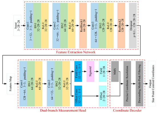
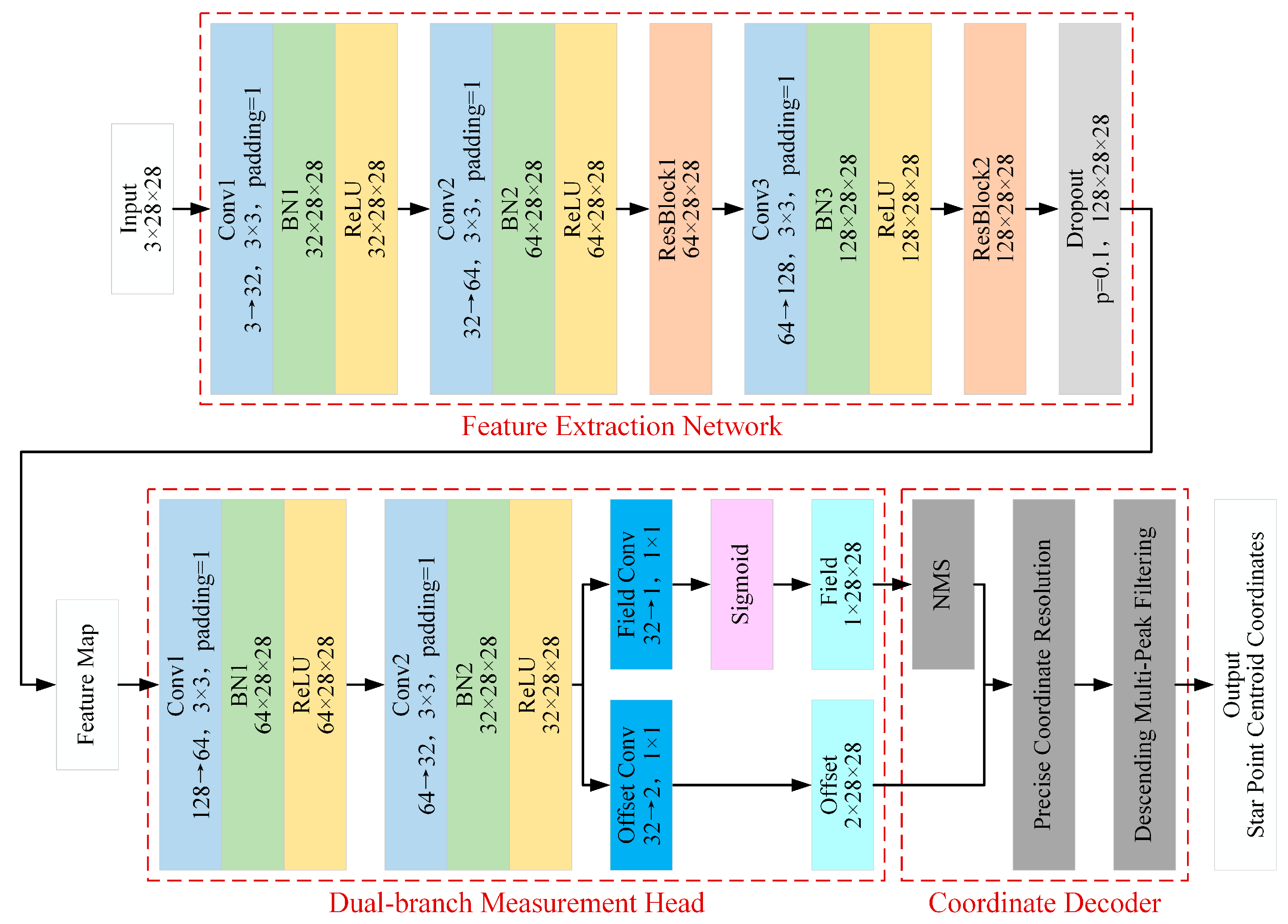
The overall architecture of the star-point centroid measurement network designed in this paper is illustrated in Figure 1. During inference, the network comprises three core components: a feature extraction network, a dual-branch measurement head (including an energy-distribution-aware probability heatmap branch and a geometry-quantization-compensated subpixel regression branch), and a coordinate decoder. During training, to address extreme positive-negative sample imbalance in severely degraded environments and suppress interference from complex noise (e.g., strong stray light and hot pixels), we design a multi-task joint loss function. This loss function drives network weight updates via backpropagation, enabling accurate perception of global energy distributions and high-precision regression of subpixel-level displacements. Overall, through an end-to-end lightweight structural design, the network aims to achieve highly robust subpixel measurements under complex and variable operating conditions while satisfying the real-time inference requirements of star sensors.

Figure 1. Overall network architecture.

2.2. Feature Extraction

In astronomical star maps, stray light and detector noise commonly interfere. The feature extraction network’s core objective is to map the input star map (3 × 28 × 28 tensor) into a high-dimensional feature space while suppressing background disturbances through effective filtering.

Given the high sensitivity of star point localization tasks to spatial details, we employ a full-resolution feature-preservation design. The processing pipeline encompasses initial convolution, feature enhancement, two residual extraction modules, and feature dimensionality expansion. All convolutional kernels use a size of 3 × 3, a stride of 1, and padding of 1, avoiding spatial quantization errors from downsampling operations such as pooling and retaining the structural characteristics of star point spread distributions. This design aligns with the core idea of high-resolution representation learning [30], which maintains high-resolution features throughout training to prevent irreversible loss of spatial information caused by low-resolution bottlenecks.

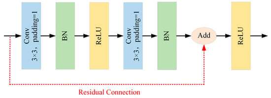
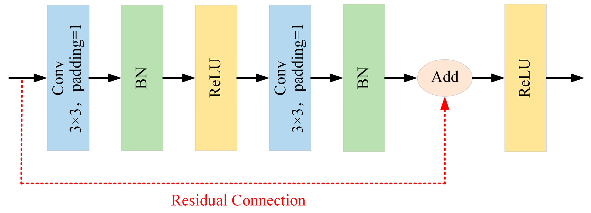
Because star points appear as energy-concentrated point targets, we mitigate receptive-field redundancy in deep network architectures by applying lightweight expansion only along the channel dimension, with feature dimensions evolving sequentially as 3→32→64→128, reducing inference overhead. To mitigate gradient attenuation with increased network depth, we embed residual blocks [31] after the output layers corresponding to 64 and 128 channels, as illustrated in Figure 2. The identity mapping component within the residual structure facilitates the lossless cross-layer transmission of the morphological features of the star point main body. At the same time, the intra-block convolutions learn residual feature corrections. This mechanism actively counteracts feature-distribution distortions induced by disturbances such as shot noise and radiometric hot pixels, thereby enhancing the model’s feature-representation capability in degraded star maps.

Figure 2. Residual block.

Furthermore, batch normalization [32] and ReLU activation functions are applied after each convolutional layer across all levels to normalize feature distributions, mitigate covariate shift, and ensure training stability. At the terminal of the feature extraction backbone network, a two-dimensional dropout [33] with a local zeroing probability of 0.1 is introduced. By randomly blocking feature channels, the network is forced to reduce its overreliance on locally abnormal activations, thereby enhancing its robustness to local extreme noise.

Regarding noise transmission in the full-resolution architecture, although no downsampling is applied, the cascaded 3 × 3 convolutions inherently act as local low-pass filters that attenuate high-frequency shot noise while preserving the low-frequency energy distribution of star spots. Meanwhile, the improved focal loss incorporated into heatmap supervision prevents the gradient contributions of massive noisy background pixels from overwhelming the star-point supervision during training, so that noise interference is suppressed at both the feature-extraction and optimization levels.

2.3. Energy Distribution-Aware Probability Heatmap Branch

In object detection tasks, bounding boxes are conventionally used for object region regression; however, this approach does not align with the physical nature of star points, which lack distinct geometric edges. The optical system’s PSF inherently modulates the energy distribution of star points received by the star sensor detector. Thus, we propose an energy distribution-aware probability heatmap branch, where pixel-level probability density prediction replaces geometric bounding-box enclosure. In recent years, the detection paradigm that characterizes target locations via keypoint heatmaps [34,35] has proven effective in general visual tasks. In this paper, we apply this approach to the star centroid measurement task and tailor the design to the physical distribution properties of star energy.

This branch operates on the 128-dimensional feature map output by the feature extraction network: first, a dimensionality-reduction convolution reduces the channels to 32; then, a 1 × 1 convolution followed by a Sigmoid activation produces a single-channel probability heatmap, denoted $\widehat{\mathrm{Y}}\in {\left[0,1\right]}^{W\times H}$.

During model training, to supervise this branch’s learning, we map ground-truth star-point coordinates to probability-distribution labels. The absolute coordinates of the true centroid of the star point in the image coordinate system are denoted as (x_c,y_c), and its discrete projection index on the feature map is denoted as $\left(\tilde{x},\tilde{y}\right)=\left(⌊x_{\mathrm{c}}⌋,⌊y_{\mathrm{c}}⌋\right)$. A symmetric two-dimensional Gaussian kernel free from spatial distortion is employed to characterize the energy distribution prior of the star point on the ideal focal plane. The target probability density Y_xy at an arbitrary spatial position (x,y) on the ground-truth probability heatmap is Y defined as:

$$Y_{\mathit{xy}}=\exp \left(-{\displaystyle \frac{{\left(x-\tilde{x}\right)}^2+{\left(y-\tilde{y}\right)}^2}{2{\sigma }_{\mathrm{p}}^2}}\right)$$

(1)

where σ_p is the standard deviation of the star point energy diffusion.

The label is generated by sampling the continuous Gaussian kernel at pixel centers rather than by integrating the density over pixel areas. The deviation between the two is analytically bounded: integration over a one-pixel-wide bin is equivalent to convolving the kernel with a uniform kernel of variance 1/12, corresponding to a relative second-moment deviation of about 33% at σ_p = 0.5. This approximation affects only the second moment of the label and does not alter the supervised energy topology, namely the peak position and monotonic decay, while the subpixel accuracy of the final centroid is compensated by the offset regression branch.

This mechanism constrains the network to not only localize the star point center but also to implicitly learn the local gradient features of Gaussian-diffused spots. As a result, even with background shot noise, the network can still accurately identify pixel clusters that exhibit the properties of real optical energy distributions.

2.4. Geometric Quantization Compensation Subpixel Regression Branch

Constrained by the spatially discrete sampling nature of the detector’s focal plane array, the extremum coordinate $\left(\widehat{x},\widehat{y}\right)$ identified by the probability heatmap branch is inherently an integer-level grid index. This unavoidable spatial quantization introduces rounding and truncation errors, confining the measurement results to the integer-pixel level. We propose a geometric quantization compensation subpixel regression branch that, based on shared features, preserves both positive and negative displacement values via a 1 × 1 purely linear convolution and outputs a two-channel offset feature map $\widehat{\mathrm{O}}\in {ℝ}^{2\times W\times H}$.

The supervision target of this branch is the local geometric truncation residual between the true continuous coordinates of star points and their discrete grid anchors. For the true star point at position (x_c,y_c), the ground-truth values of subpixel quantization compensation $O_{\tilde{x}\tilde{y}}$ in the horizontal and vertical directions are defined as:

$$O_{\tilde{x}\tilde{y}}=\left[\begin{array}{l}\Delta x\\ \Delta y\end{array}\right]=\left[\begin{array}{l}{x}_{\mathrm{c}}-\tilde{x}\\ y_{\mathrm{c}}-\tilde{y}\end{array}\right]\Delta x,\Delta y\in \left[0,1\right)$$

(2)

During the inference phase, the network first performs non-maximum suppression (NMS) on the probability heatmap $\widehat{\mathit{Y}}$ to localize the integer coordinates $\left(\widehat{x},\widehat{y}\right)$ corresponding to the strongest response peak. Subsequently, it extracts the predicted compensation value (δx,δy) from the same spatial index in the offset feature map $\widehat{\mathit{O}}$. Finally, the centroid coordinates (x_sub,y_sub) of the star point can be computed as follows:

$$x_{\mathrm{sub}}=\widehat{x}+\delta x$$

(3)

$$y_{\mathrm{sub}}=\widehat{y}+\delta y$$

(4)

Since the supervision anchor in Equation (2) is defined by flooring the ground-truth centroid, the offset labels are always non-negative and lie in [0, 1). At inference, however, the peak selected by NMS is the pixel with the highest predicted probability, which is not necessarily the anchor: when the fractional part of the true coordinate exceeds 0.5, the true centroid is geometrically closer to the pixel adjacent to the anchor, the Gaussian label assigns a higher response to that neighboring pixel, and the predicted peak tends to shift accordingly, so the compensation required at the shifted peak is negative. The signed, activation-free linear output of this branch accommodates exactly this case.

This dual-branch orthogonal design decouples the non-convex and complex star-point prediction task into explicit region energy perception and linear geometric compensation within a minimal range. The subpixel regression branch eliminates the need to focus on global background noise filtering; instead, it focuses solely on fitting local bias residuals, ensuring accurate star-centroid measurements with minimal additional parameters.

2.5. Loss Function

To enable efficient end-to-end training of the aforementioned dual-branch network architecture, a multi-task joint loss function is designed. The total loss function L_total consists of three components: energy-aware heatmap loss L_hm, subpixel geometric offset loss L_off, and physical centroid loss L_center. Its calculation formula is given as follows:

L_total = λ₁L_hm + λ₂L_off + λ₃L_center

(5)

where λ₁, λ₂, and λ₃ are fixed hyperparameter weights that balance the loss gradients of the individual tasks; they are kept constant throughout training.

2.5.1. Energy-Aware Heatmap Loss

In star maps, the ratio of star point targets to deep-space background typically exhibits extreme positive-negative sample imbalance. To avoid the deep-space background dominating the network gradient, an improved focal loss function [36] is incorporated into heatmap supervision, and its calculation formula is given below:

$$L_{\mathrm{hm}}=-{\displaystyle \frac{1}{\omega +1}}\left[{\displaystyle \frac{\omega }{N_{\mathrm{pos}}}}{\displaystyle {\displaystyle \sum _{x=1}^W}{\displaystyle \sum _{y=1}^H{\left(1-{\widehat{Y}}_{\mathit{xy}}\right)}^{\alpha }}}\log \left({\widehat{Y}}_{\mathit{xy}}\right)+{\displaystyle \frac{1}{N_{\mathrm{neg}}}}{\displaystyle {\displaystyle \sum _{x=1}^W}{\displaystyle \sum _{y=1}^H{\left(1-Y_{\mathit{xy}}\right)}^{\beta }}}{\left({\widehat{Y}}_{\mathit{xy}}\right)}^{\alpha }\log \left(1-{\widehat{Y}}_{\mathit{xy}}\right)\right]$$

(6)

where ${\widehat{Y}}_{\mathit{xy}}$ and Y_xy are the predicted probability response and the ground-truth Gaussian distribution probability label at the spatial coordinate (x,y) of the feature map, respectively; N_pos is the number of ground-truth star points in the star map; α and β are hyperparameters that respectively regulate the penalty weights for samples with varying difficulty levels; ω = 100 is the asymmetric weight applied to the positive-sample term; N_neg is the number of background pixels with Y_xy < 1. The positive and negative terms are normalized separately by N_pos and N_neg, respectively, i.e., class-wise decoupled normalization.

The energy-aware heatmap loss mitigates gradient imbalance caused by the large proportion of background pixels by down-weighting easily separable background samples, thereby encouraging the network to prioritize hard-to-classify faint star targets during training.

The focusing parameter α = 2 follows the recommendation of the original focal loss [36]. The balancing factor β = 4 is set to further strengthen the gradient contribution of the positive-sample domain, compensating for the extreme scarcity of star-point pixels relative to the deep-space background. The value β = 4 follows the established practice in keypoint heatmap supervision [34,35].

2.5.2. Subpixel Geometric Offset Loss

For the geometric quantization-compensated subpixel regression branch, given that its prediction target is a subpixel offset constrained within interval [0, 1), direct adoption of absolute error (AE) or mean squared error (MSE) exhibits inherent limitations. To enable faster convergence in the early training phase and maintain gradient smoothness to avoid oscillations as it approaches the target in the later phase, the Smooth L1 loss function [37] is used to constrain the two-channel offset feature maps. Its calculation formula is given as follows:

$$L_{\mathrm{off}}={\displaystyle \frac{1}{N_{\mathrm{pos}}}}{\displaystyle \sum _{(x,y)\in \mathrm{M}}{\displaystyle \sum _{c\in \left\{x,y\right\}}\mathrm{Smooth}}\mathrm{L}1}({\widehat{O}}_{\mathit{xy}}^c,O_{\mathit{xy}}^c)$$

(7)

$$\mathrm{SmoothL}1(d)=\left\{\begin{array}{ll}0.5d^2,\hfill & \left|d\right|<1\hfill \\ \left|d\right|-0.5,\hfill & \left|d\right|\ge 1\hfill \end{array}\right.$$

(8)

where M is a mask set consisting solely of discrete coordinates of real star points (i.e., regression errors in non-star regions are excluded from backpropagation); ${\widehat{O}}_{\mathit{xy}}^c$ and $O_{\mathit{xy}}^c$ are the corresponding scalar values of the predicted and ground-truth subpixel offsets at node (x,y) along channel c; d is the regression residual derived from the subtraction of the two values.

Restricting the regression supervision to the discrete anchor coordinates of star points follows the standard practice of keypoint-based detection paradigms such as CenterNet [35], in which the offset is defined only at the target location, and supervising neighboring pixels would introduce semantic ambiguity. Neighborhood information is nevertheless exploited implicitly through the shared backbone features, since the receptive field of the regression branch covers the entire star spot.

2.5.3. Physical Centroid Loss

While L_hm and L_off can independently guide network convergence within their respective feature spaces, this setup still leaves the network without a global error constraint on the absolute position of the final target output. To address this issue, this paper introduces a physical centroid loss based on Euclidean distance. After dynamically predicting coordinates during forward propagation, we directly compute the Euclidean distance between these predicted coordinates and the ground-truth subpixel coordinates. Its calculation formula is given as follows:

$$L_{\mathrm{center}}={\displaystyle \frac{1}{N_{\mathrm{valid}}}}{\displaystyle \sum _{k=1}^{N_{\mathrm{valid}}}\sqrt{{(x_{\mathrm{sub},k}-x_{\mathrm{c},k})}^2+{(y_{\mathrm{sub},k}-y_{\mathrm{c},k})}^2}}$$

(9)

where N_valid is the count of effective initial predicted centroids for which the network response probability exceeds a preset threshold; (x_sub,k,y_sub,k) is the predicted coordinates of the k-th star point corresponding to the label in the dataset; (x_c,k,y_c,k) is the ground-truth coordinates of the k-th star point corresponding to the label in the dataset.

Regarding gradient propagation, the peak selection involved in Equation (9) is a hard, non-differentiable operation, and the selected integer coordinates are treated as constants during backpropagation, consistent with the standard practice in keypoint-based detection paradigms. The gradients of the centroid loss flow into the predicted compensation values δx and δy at the selected peak location through differentiable indexing of the offset feature map $\widehat{\mathit{O}}$, and further back into the offset head and the shared backbone features at that spatial location. The two supervision signals thus act in a complementary division of labor: the heatmap loss independently determines where the peak is located at the integer level, while the centroid loss constrains the final decoded coordinate at the subpixel level on the network’s own predicted peak. This design exactly matches the decoding pathway defined by Equations (3) and (4) at inference, closing the train–inference gap that would otherwise arise because the offset loss is defined only at the ground-truth anchor.

The physical centroid loss directly imposes supervisory constraints on the final resolved subpixel continuous coordinates, mitigating cumulative errors introduced during stepwise parameter estimation and further improving star-centroid localization accuracy.

The loss weights are set to λ₁ = 1 and λ₂ = λ₃ = 0.1, so that the heatmap supervision, which carries the primary detection signal, dominates the joint optimization, while the offset and centroid losses serve as geometric constraints of moderate strength. Since each 28 × 28-pixel window contains exactly one star point, non-maximum suppression of the heatmap produces a single peak per window, and the centroid loss is computed as a direct one-to-one matching between this peak and the ground-truth centroid, without any multi-target assignment. During training, the activation threshold of the physical centroid loss is unified with the detection threshold, both set to 0.2. The centroid loss is activated only for samples whose peak heatmap confidence exceeds 0.2, while the heatmap and offset losses remain active for all samples, so that every sample still receives primary supervision and the optimization direction is not altered.

At inference, the centroid is decoded by thresholding the heatmap response at 0.2, detecting the peak position, and compensating the integer peak coordinate with the predicted subpixel offset, as defined in Equations (3) and (4).

3. Results

3.1. Star Map Dataset

In practical applications of star sensors, acquiring large-scale, real-world captured datasets with ground-truth star centroid values is challenging. Therefore, based on the PSF and detector noise model, this paper constructs a dataset of 300,000 simulated star maps, each with a resolution of 28 × 28 pixels.

3.1.1. Calculation of Discrete Energy Distribution of Star Points

To realistically simulate the energy dispersion of starlight on the focal plane of the detector after passing through the optical system, the differential form of the two-dimensional Gaussian cumulative distribution function [38] is employed to perform a double integral over the number of photons incident on a specific pixel, i.e.,

$$E(u,v)={\displaystyle {\int }_u^{u+1}{\displaystyle {\int }_v^{v+1}\frac{1}{2\pi {\sigma }_x{\sigma }_y}}}\exp \left(-{\displaystyle \frac{{(x-x_{\mathrm{c}})}^2}{2{\sigma }_x^2}}-{\displaystyle \frac{{(y-y_{\mathrm{c}})}^2}{2{\sigma }_y^2}}\right)\mathrm{d}x\mathrm{d}y$$

(10)

where (x_c,y_c) is the ground-truth centroid of the star point; σ_x and σ_y are the standard deviations of the Gaussian dispersion kernel along two orthogonal directions.

During star map data generation, an error function is introduced to analytically solve the double integral, and asymmetric distortion and rotation parameters are injected with a specific probability to simulate optical system aberrations.

The asymmetric distortion is injected with condition-dependent probabilities of 0.1, 0.35, and 0.6 for the ideal, typical, and extreme conditions, respectively, under which the star spot is rendered as an elliptical Gaussian with unequal major and minor axes and a random rotation angle uniformly sampled from 0° to 180°. These probabilities are empirical engineering settings and have not been calibrated against on-orbit measured data.

3.1.2. Noise Modeling and Operating Condition Grading

To comprehensively assess the network’s generalization bounds under varying operating conditions, we categorize the dataset into three types based on distinct operating-environment classifications, with 100,000 star maps independently generated for each type. Based on the detector noise model, the SNR of star points is defined as:

$$\mathit{SNR}={\displaystyle \frac{S_{\mathrm{total}}}{\sqrt{S_{\mathrm{total}}+N_{\mathrm{pix}}({\mu }_{\mathrm{bg}}+{\sigma }_{\mathrm{read}}^2)}}}$$

(11)

where S_total is the number of signal electrons of the star point; N_pix is the total number of pixels occupied by a star point; μ_bg is the mean value of the background noise; σ_read is the standard deviation of the detector readout noise.

The detector noise is modeled as a mixture of Poisson noise from the signal and background and Gaussian readout noise. In the signal-dominated regime, the mixture approximates a Gaussian distribution and Equation (11) holds directly; in the low-signal regime, where the Poisson component dominates, Equation (11) still preserves the correct order-of-magnitude relationship. Regarding boundary conditions, when dark current and readout noise dominate, Equation (11) degenerates to a form determined by the background mean and readout variance.

The parameter settings of the simulated star maps under three operating conditions are presented in Table 2.

Table 2. The parameter settings of the simulated star maps under three operating conditions.

Operating Conditions	Data Category	Signal Photon	Background Photons Mean Value	Readout Noise	Hot Pixel Injection Probability
Ideal environment (e.g., dark background)	Setting_A	4000–8000	20	3	5%
Typical environment (e.g., moderate stray light)	Setting_B	1000–4000	60	10	30%
Extreme environment (e.g., high-radiation conditions)	Setting_C	200–800	120	20	80%

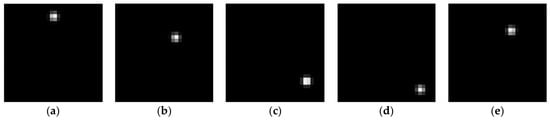
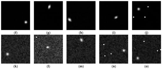
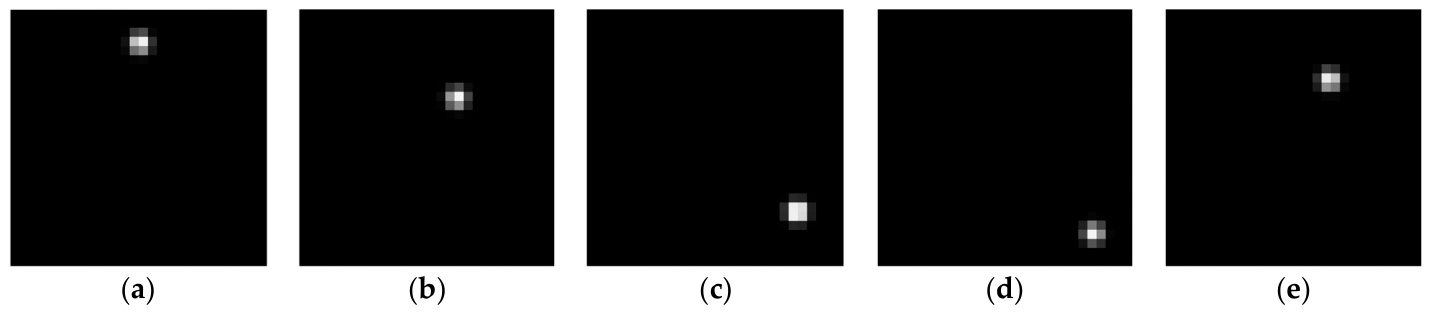
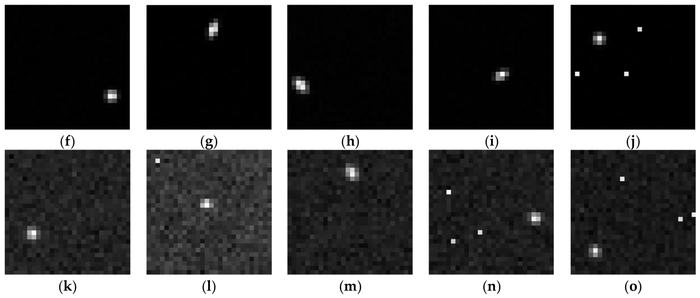
Examples of simulated star maps under the three operating conditions are presented in Figure 3.

Figure 3. Simulated star maps under three operating conditions. (a–e) Setting_A; (f–j) Setting_B; (k–o) Setting_C.

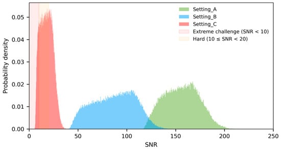
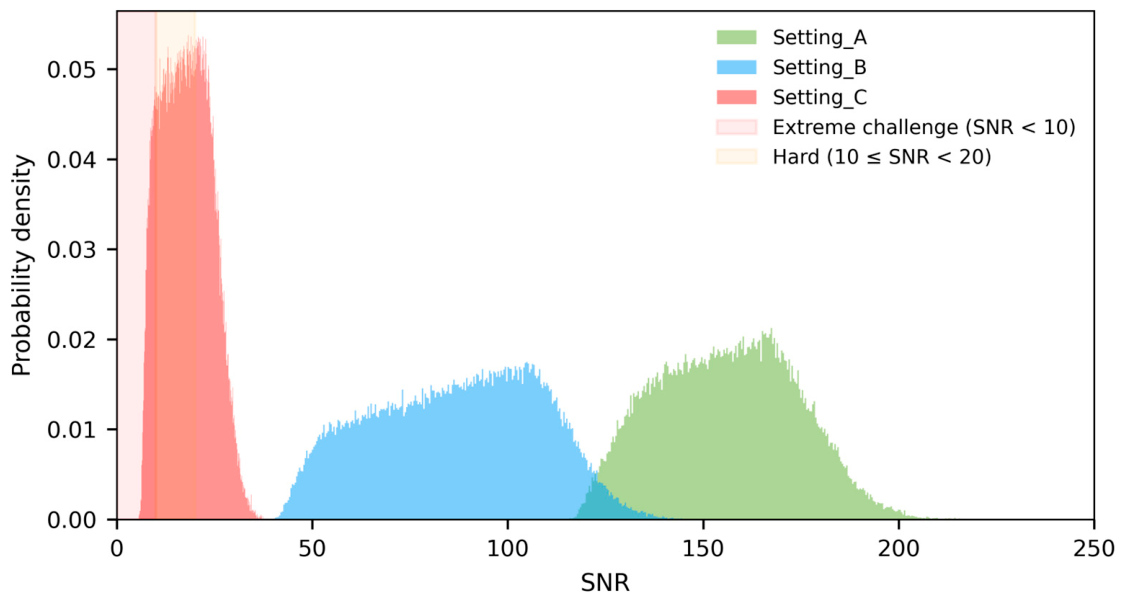
The probability density distribution of the SNR of simulated star maps under three operating conditions is presented in Figure 4. The average SNR under typical conditions is 86.91, while under extreme conditions it drops to 17.85; in particular, the proportion of weak-signal regions with SNR < 10, where traditional centroid methods are highly susceptible to failure, reaches 12.09%. These characteristics provide a data basis for verifying the robustness of the proposed method.

Figure 4. Probability density distribution of SNR in simulated star maps.

3.2. Training Parameters

The 300,000 simulated star maps were randomly partitioned at the condition level into three mutually exclusive subsets at a ratio of 70%/15%/15%: 210,000 maps for training (70,000 per condition), 45,000 for validation (15,000 per condition), and 45,000 for independent testing (15,000 per condition). The validation set was used exclusively for early stopping and model selection, whereas the test set remained completely untouched throughout training, model selection, and hyperparameter analysis, and was used exclusively for reporting the final performance metrics. All hyperparameter sensitivity experiments in Section 3.4.3 are reported on the validation set. Prior to input into the network, pixel values of single-channel grayscale images were linearly normalized and mapped to the dimensionless interval [−1, 1], aiming to accelerate the convergence of activation functions in each convolutional layer. To enhance the model’s generalization ability against background disturbances, an online data augmentation strategy with a 50% probability was configured during training. Specifically, Gaussian white noise with a standard deviation of 0.05 and contrast perturbations within the ratio range of 0.8 to 1.2 were randomly applied to the star maps during training iterations.

The model is constructed based on the PyTorch 2.11.0 deep learning framework [39] with CUDA 12.8 (NVIDIA Corporation, Santa Clara, CA, USA). Model training was carried out on a server equipped with 8 NVIDIA GeForce RTX 4090 GPUs (NVIDIA Corporation, Santa Clara, CA, USA), while inference latency testing was performed on a single NVIDIA GeForce RTX 4090 GPU in a single-frame mode with a batch size of 1—this setup closely mimics the actual frame-by-frame processing workflow of star sensors. The traditional centroid-based methods involved in the comparative experiments were executed and timed on an Intel Xeon Platinum 8368Q CPU with a base clock speed of 2.60 GHz. To ensure the reproducibility of the experimental results, the global random seed was fixed at 42. The AdamW optimizer [40] was adopted for model training, with a batch size of 64, an initial learning rate of 5 × 10⁻⁶, and a weight decay coefficient of 1 × 10⁻⁶. A cosine annealing strategy was employed to dynamically and smoothly decay the learning rate to 1 × 10⁻⁶. To mitigate gradient explosion induced by noise, gradient clipping with a threshold of 1 was enforced. An early stopping mechanism with a patience value of 5 was incorporated during training, which automatically monitors the multi-task joint loss on the validation set after each epoch. When the loss ceases to decrease, the iteration is immediately terminated, and the model weights corresponding to the minimum validation error are saved as the optimal model weights. Furthermore, the confidence threshold for star point detection is set to 0.2. The detailed training parameter settings are summarized in Table 3.

Table 3. Specific training parameters settings.

Configuration	Setting
Optimizer	AdamW
Initial learning rate	5 × 10−6
Weight decay coefficient	1 × 10−6
Learning strategy	Cosine annealing
Batch size	64
Maximum iterations	20
Gradient clipping	1
Early stopping epochs	5
Focal loss focusing parameter α	2
Focal loss balancing factor β	4
Energy-aware heatmap loss weight λ1	1
Subpixel geometric offset weight λ2	0.1
Physical centroid loss weight λ3	0.1
Asymmetric weight for positive samples in focal loss	100
Gaussian kernel standard deviation for heatmap labels σp	0.5
Confidence threshold for star point detection	0.2

3.3. Evaluation Metrics

To scientifically and comprehensively evaluate the performance of star centroid measurement methods, an evaluation framework is constructed, encompassing key metrics including detection rate, mean error, median error, standard deviation, and average computation time.

Let the test set contain a total of N star maps. The number of star maps with successfully detected star points is denoted as N_v, and the corresponding set of indices of these star maps is denoted as V. For the i-th (i ∈ V) successfully detected star map, the calculation formula for the centroid measurement error of its star points is given as follows:

$$e_i=\sqrt{{\left(x_{\mathrm{sub},i}-x_{c,i}^{\ast }\right)}^2+{\left(y_{\mathrm{sub},i}-y_{c,i}^{\ast }\right)}^2}$$

(12)

where e_i is the centroid measurement error of the star points in the i-th star map; x_sub,i and y_sub,i are the predicted horizontal (x-axis) and vertical (y-axis) coordinates of the star point, respectively; $x_{c,i}^{\ast }$ and $y_{c,i}^{\ast }$ are the ground-truth horizontal (x-axis) and vertical (y-axis) coordinates of the star point, respectively.

3.3.1. Detection Rate

The detection rate is the percentage of star maps in which star points are successfully identified and their coordinates extracted, relative to the total number of star maps. It characterizes the star centroid measurement method’s ability to detect star points under noise. The calculation formula is given as follows:

$$\mathit{DR}={\displaystyle \frac{N_{\mathrm{v}}}{N}}\times 100\%$$

(13)

where DR is the detection rate.

3.3.2. Mean Error

Mean error is defined as the arithmetic mean of centroid measurement errors across all successfully detected maps. It characterizes the overall measurement accuracy of the star centroid measurement method. The calculation formula is given as follows:

$$\overline{e}={\displaystyle \frac{1}{N_{\mathrm{v}}}}{\displaystyle \sum _{i\in V}{e}_i}$$

(14)

where $\overline{e}$ is the mean error.

3.3.3. Median Error

Median error is the middle value of the centroid measurement error set for all successfully detected star maps, sorted in ascending order. This metric characterizes the more objective and representative measurement performance of most star maps when the error distribution deviates from the typical distribution or contains extreme outliers (e.g., severe deviations induced by hot pixels). $E_{\mathrm{sort}}=\left\{e_{\left(1\right)}\le e_{\left(2\right)}\le \cdots \le e_{\left(N_v\right)}\right\}$ denotes the error sequence sorted in ascending order; its calculation formula is given as follows:

$$\mathit{Me}{d}_{\mathrm{e}}=\left\{\begin{array}{l}{e}_{\left(k+1\right)}\hspace{1em}\hspace{1em}\hspace{1em}\hspace{1em},N_{\mathrm{v}}=2k+1\\ {\displaystyle \frac{1}{2}}\left[e_{\left(k\right)}+e_{\left(k+1\right)}\right] ,N_{\mathrm{v}}=2k\end{array}\right., k\in {\mathbb{N}}^{+}$$

(15)

where Med_e is the median error; e_(k) is the measurement error at the k-th position in the ascendingly sorted sequence.

3.3.4. Standard Deviation

Standard deviation is the root mean square (RMS) of measurement-error deviations from the mean error. In metrology, this metric characterizes the Type A uncertainty of a measurement method: a smaller value indicates stronger anti-disturbance capability and greater measurement stability. Its calculation formula is given as follows:

$${\sigma }_{\mathrm{e}}=\sqrt{{\displaystyle \frac{1}{N_{\mathrm{v}}-1}}{{\displaystyle \sum _{i\in V}\left(e_i-\overline{e}\right)}}^2}$$

(16)

where σ_e is the standard deviation.

3.3.5. Average Inference Time

Average inference time is the mean single-frame inference execution time across all star maps in the test set. This metric reflects the method’s engineering feasibility for real-time execution on a target hardware platform. Its calculation formula is given as follows:

$$T_{\mathrm{avg}}={\displaystyle \frac{1}{N}}{\displaystyle \sum _{i=1}^N{t}_i}$$

(17)

where T_avg is the average inference time per frame on the test set; t_i is the time consumed for processing the i-th single-frame star map. To mitigate hardware initialization jitter, five warm-up inference runs are executed prior to formal timing, and the timing interval is restricted to the network forward propagation phase.

3.4. Results Analysis

3.4.1. Experimental Results of the Proposed Method

The star centroid measurement results of the proposed method on the independent star-map test sets with varying degradation levels are presented in Table 4.

Table 4. Star centroid measurement results across star map data categories with varying degradation levels.

Category	Detection Rate (%)	Mean Error (Pixel)	Median Error (Pixel)	Standard Deviation (Pixel)	Error > 0.5 Pixels (%)	Error > 1 Pixel (%)	Average Inference Time (ms)
Setting_A	100	0.0096	0.0089	0.0052	0.00	0.00	1.07
Setting_B	100	0.0151	0.0136	0.0089	0.00	0.00	1.07
Setting_C	100	0.0576	0.0486	0.0397	0.00	0.00	1.07
Overall *	100	0.0274	0.0151	0.0320	0.00	0.00	1.07

* Overall represents a weighted aggregation of the results across the three data categories.

The detection rate reaches 100% under all three operating conditions. Under ideal conditions, the probability heatmap branch accurately captures the energy distribution characteristics of the optical PSF of star points, and the subpixel regression branch effectively mitigates quantization errors introduced by the detector’s discrete spatial sampling, enabling high-precision measurements at the 1/100-pixel scale. Under typical conditions, the heatmap branch effectively suppresses shot-noise-induced distortion of the star-point energy distribution, with no significant degradation in measurement accuracy, verifying the generalization capability of the method. Under extreme conditions, the dual-branch network distinguishes stars with multi-pixel energy distributions from hot pixels characterized by single-pixel amplitude anomalies, thereby avoiding false alarms while preserving centroid measurement accuracy.

Based on the results on the independent test set across the three data categories, the proposed method achieves a 100% star detection rate on 45,000 test star maps, with an overall mean error of 0.0274 pixels, an overall median error of 0.0151 pixels, and an overall standard deviation of 0.0320 pixels. The median error is markedly lower than the mean error, indicating a right-skewed distribution of overall errors, i.e., most star maps have measurement errors substantially smaller than the overall average. Regarding real-time performance, the per-frame inference time averages 1.07 ms over all 45,000 test frames, with a median of 1.05 ms, a 99th percentile of 1.21 ms, and a standard deviation of 0.32 ms, corresponding to a processing rate of approximately 938 frames per second (fps). Only 5 frames, i.e., 0.011%, exceed 2 ms, and a single isolated frame of approximately 67 ms alone accounts for 95.8% of the reported variance; excluding this frame, the standard deviation of the remaining frames is approximately 0.065 ms. Even that isolated worst case remains below the typical 100 ms sampling period of star sensors. Since the computation graph is constant for the fixed 28 × 28 input with no data-dependent iterations, the latency variation is attributable to the execution environment of the general-purpose platform rather than to the algorithm itself. The complete pipeline—image reading, preprocessing, network forward pass, NMS, and offset decoding—averages 1.62 ms per frame (99th percentile 1.81 ms).

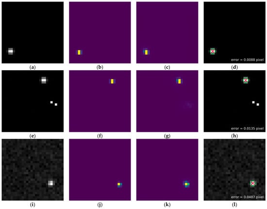
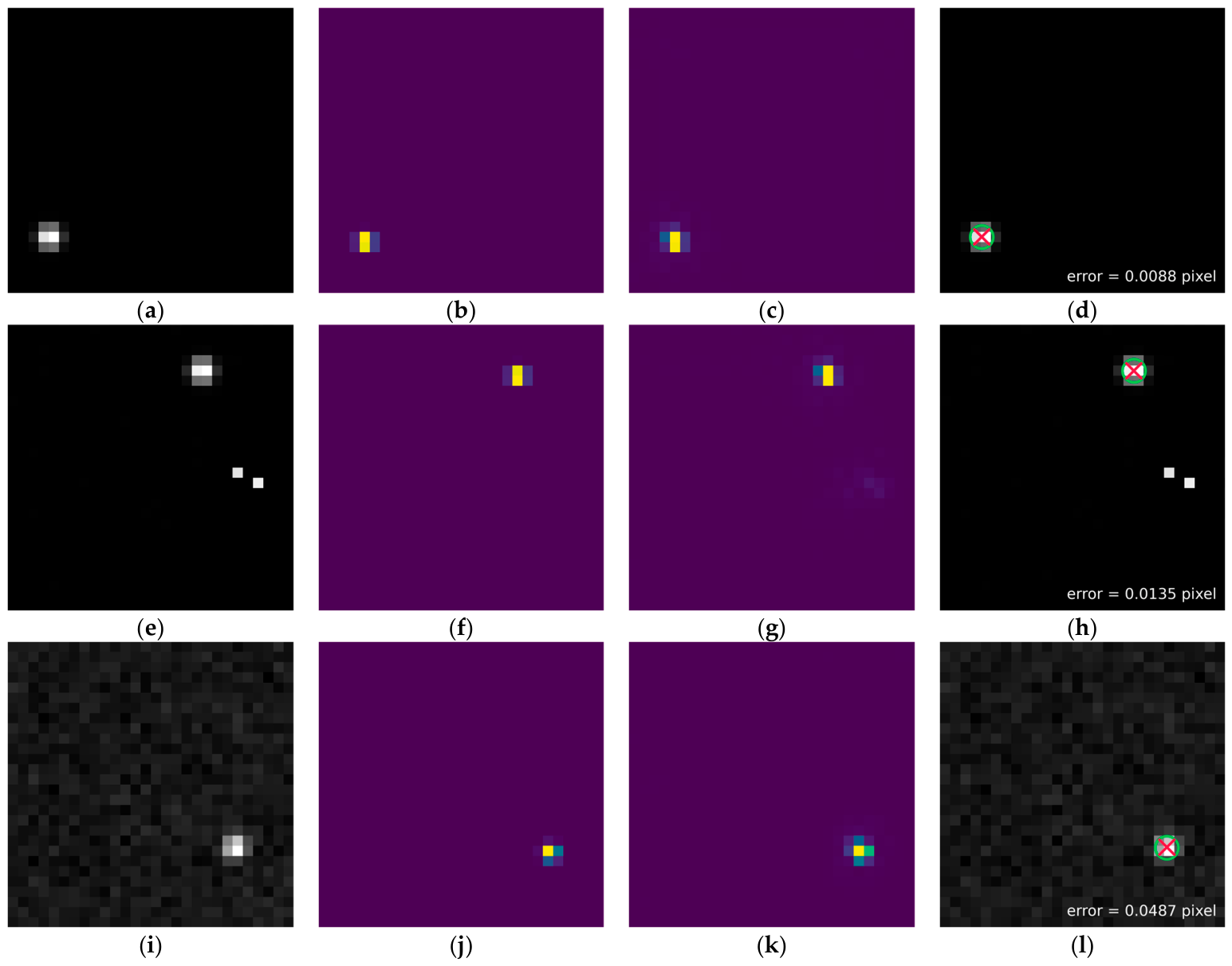
Qualitative localization results under the three operating conditions are illustrated in Figure 5. The predicted probability heatmaps closely match the ground-truth Gaussian heatmaps under all three conditions. Even under Setting_C, the weak responses at hot-pixel locations remain well below the star-point peak and are excluded by the detection threshold. The predicted centroids (red cross) almost coincide with the ground truth (green circle), with per-sample errors of only 0.0088, 0.0135, and 0.0487 pixels for the representative samples shown.

Figure 5. Qualitative localization results under the three operating conditions. (a–d) Setting_A; (e–h) Setting_B; (i–l) Setting_C. For each condition, input star map, ground-truth Gaussian heatmap, predicted probability heatmap, and localization overlay, where the green circle denotes the ground-truth centroid and the red cross denotes the predicted centroid.

3.4.2. Comparison with Existing Methods

To objectively evaluate the proposed method’s performance, we selected four classical star centroid extraction methods for comparative experiments: the centroid method, threshold-based centroid method, squared-weighted centroid method, and Gaussian surface fitting method. We conducted the comparative experiments on the same independent test set as the proposed method, and present the results in Table 5. In addition to the four classical methods, a U-Net heatmap baseline with 467,809 parameters was trained under the identical protocol and included in the comparison. Moreover, a CenterNet-style heatmap–offset baseline [35] with 186,243 parameters—featuring a two-stage stride-2 downsampling backbone, dual heatmap–offset decoding heads, the same heatmap supervision and Smooth L1 offset loss, and no physical centroid loss—was implemented under the same framework and training protocol. Since absolute errors are not directly comparable across studies due to differences in datasets, star sizes, and task definitions, all learning-based comparisons in this work were performed on the same dataset under the same partition protocol.

Table 5. Star centroid measurement results of the comparison methods on the independent test set.

Method	Data Category	Detection Rate (%)	Mean Error (Pixel)	Median Error (Pixel)	Standard Deviation (Pixel)	Error > 0.5 Pixels (%)	Error > 1 Pixel (%)	Average Inference Time (ms)
Centroid method	Setting_A	100	0.0147	0.0088	0.3141	0.02	0.02	0.15
	Setting_B	100	0.0835	0.0501	0.7730	0.21	0.14	0.15
	Setting_C	100	0.3167	0.2319	1.2830	1.23	0.45	0.15
	Overall *	100	0.1383	0.0492	0.8930	0.48	0.20	0.15
Threshold-based centroid method	Setting_A	100	0.0121	0.0066	0.3144	0.02	0.02	0.16
	Setting_B	100	0.0448	0.0135	0.7814	0.21	0.14	0.16
	Setting_C	100	0.1745	0.0766	1.3343	0.50	0.45	0.16
	Overall *	100	0.0771	0.0144	0.9137	0.24	0.20	0.16
Squared-weighted centroid method	Setting_A	100	0.0186	0.0134	0.3144	0.02	0.02	0.16
	Setting_B	100	0.0484	0.0176	0.7815	0.21	0.15	0.16
	Setting_C	100	0.1457	0.0514	1.3468	0.49	0.45	0.16
	Overall *	100	0.0709	0.0198	0.9188	0.24	0.20	0.16
Gaussian surface fitting method	Setting_A	99.98	0.0081	0.0075	0.0043	0.00	0.00	1.64
	Setting_B	99.87	0.0152	0.0126	0.1453	0.01	0.01	1.62
	Setting_C	99.45	0.0668	0.0471	0.4906	0.06	0.06	1.82
	Overall *	99.76	0.0300	0.0136	0.2962	0.02	0.02	1.70
U-Net heatmap baseline	Setting_A	100	0.1044	0.0987	0.0631	0.00	0.00	1.28
	Setting_B	100	0.1052	0.0969	0.0627	0.00	0.00	1.28
	Setting_C	100	0.1256	0.1143	0.0735	0.03	0.00	1.28
	Overall *	100	0.1117	0.1040	0.0673	0.01	0.00	1.28
CenterNet-style heatmap–offset baseline [35]	Setting_A	100	0.1563	0.1206	0.1413	2.63	0.00	0.68
	Setting_B	100	0.1604	0.1238	0.1398	2.77	0.00	0.68
	Setting_C	100	0.2068	0.1679	0.1522	5.58	0.01	0.68
	Overall *	100	0.1745	0.1393	0.1463	3.66	0.00	0.68

* Overall represents a weighted aggregation of the results across the three data categories. Percentages are computed over the 15,000 test images per setting; for the Gaussian surface fitting method, they are computed over the converged samples, with diverged samples reflected in the detection rate.

Table 5. Star centroid measurement results of the comparison methods on the independent test set.

Method	Data Category	Detection Rate (%)	Mean Error (Pixel)	Median Error (Pixel)	Standard Deviation (Pixel)	Error > 0.5 Pixels (%)	Error > 1 Pixel (%)	Average Inference Time (ms)
Centroid method	Setting_A	100	0.0147	0.0088	0.3141	0.02	0.02	0.15
	Setting_B	100	0.0835	0.0501	0.7730	0.21	0.14	0.15
	Setting_C	100	0.3167	0.2319	1.2830	1.23	0.45	0.15
	Overall *	100	0.1383	0.0492	0.8930	0.48	0.20	0.15
Threshold-based centroid method	Setting_A	100	0.0121	0.0066	0.3144	0.02	0.02	0.16
	Setting_B	100	0.0448	0.0135	0.7814	0.21	0.14	0.16
	Setting_C	100	0.1745	0.0766	1.3343	0.50	0.45	0.16
	Overall *	100	0.0771	0.0144	0.9137	0.24	0.20	0.16
Squared-weighted centroid method	Setting_A	100	0.0186	0.0134	0.3144	0.02	0.02	0.16
	Setting_B	100	0.0484	0.0176	0.7815	0.21	0.15	0.16
	Setting_C	100	0.1457	0.0514	1.3468	0.49	0.45	0.16
	Overall *	100	0.0709	0.0198	0.9188	0.24	0.20	0.16
Gaussian surface fitting method	Setting_A	99.98	0.0081	0.0075	0.0043	0.00	0.00	1.64
	Setting_B	99.87	0.0152	0.0126	0.1453	0.01	0.01	1.62
	Setting_C	99.45	0.0668	0.0471	0.4906	0.06	0.06	1.82
	Overall *	99.76	0.0300	0.0136	0.2962	0.02	0.02	1.70
U-Net heatmap baseline	Setting_A	100	0.1044	0.0987	0.0631	0.00	0.00	1.28
	Setting_B	100	0.1052	0.0969	0.0627	0.00	0.00	1.28
	Setting_C	100	0.1256	0.1143	0.0735	0.03	0.00	1.28
	Overall *	100	0.1117	0.1040	0.0673	0.01	0.00	1.28
CenterNet-style heatmap–offset baseline [35]	Setting_A	100	0.1563	0.1206	0.1413	2.63	0.00	0.68
	Setting_B	100	0.1604	0.1238	0.1398	2.77	0.00	0.68
	Setting_C	100	0.2068	0.1679	0.1522	5.58	0.01	0.68
	Overall *	100	0.1745	0.1393	0.1463	3.66	0.00	0.68

* Overall represents a weighted aggregation of the results across the three data categories. Percentages are computed over the 15,000 test images per setting; for the Gaussian surface fitting method, they are computed over the converged samples, with diverged samples reflected in the detection rate.

For all classical methods, coarse localization was unified as the peak position after Gaussian smoothing with σ = 1, with a 3σ detection criterion, under which a peak below the image mean plus three standard deviations was counted as undetected. Gaussian surface fitting used the Levenberg–Marquardt algorithm implemented by the curve_fit function in the SciPy library with maxfev = 200, initialized at the coarse peak position with a 7 × 7 fitting window, while centroid-based methods used a 5 × 5 window; samples whose fit diverged or deviated from the window center by more than half the window width were excluded as undetected.

For data category Setting_A—where star point energy distributions strictly align with the prior of a Gaussian point spread function under ideal SNR conditions—the Gaussian surface-fitting method benefits from its analytical optimization model, achieving a mean error of 0.0081 pixels. The proposed method shows comparable accuracy: both effectively mitigate quantization errors from the detector’s discrete spatial sampling. While the threshold-based centroid method yields a slightly smaller median error of 0.0066 pixels, the standard deviations of all three centroid-based methods are approximately 0.31 pixels, constrained by the energy truncation effect at the edges of fixed computational windows.

For data category Setting_B—characterized by moderate SNR and stray light interference—the standard centroid method, which accumulates background noise without discrimination, exhibits an average error of 0.0835 pixels, a notable increase from ideal conditions. The threshold-based centroid method and squared-weighted centroid method, which leverage low-gray-level background suppression, constrain the average error to within 0.05 pixels; however, their standard deviations increase substantially relative to the ideal scenario. In contrast, both the proposed method and the Gaussian surface fitting method effectively mitigate shot-noise-induced energy-distribution distortions under these conditions, with no significant degradation in star-centroid measurement accuracy.

For data category Setting_C—representing extreme conditions combining low SNR with randomly distributed intense radiometric hot pixels—the standard centroid method, threshold-based centroid method, and squared-weighted centroid method fail to distinguish genuine starlight with multi-pixel features from single-pixel amplitude anomalies induced by radiometric hot pixels. The average errors of these three centroid-based methods degrade to over 0.14 pixels, while their standard deviations all exceed 1.2 pixels. Although the Gaussian surface fitting method relies on a rigorous mathematical analytical model, its nonlinear least-squares optimization process is prone to numerical divergence or convergence to local minima under interference from such single-pixel amplitude anomalies. Because of this numerical limitation, the method’s detection rate drops to 99.45%, and its measurement standard deviation increases to 0.4906 pixels. In contrast, the proposed dual-branch network maintains a 100% detection rate and a measurement standard deviation of only 0.0397 pixels, about 1/12 that of the Gaussian surface fitting method.

The unusually large standard deviations of the classical methods relative to their means arise from heavy-tailed error distributions: the vast majority of samples achieve errors at the 0.01-pixel level, as evidenced by the medians in Table 5, while rare gross errors, mainly hot-pixel mis-locking in centroid-based methods and fitting divergence in Gaussian fitting, dominate the standard deviations. The two columns added to Table 5 quantify the frequency of these extreme errors. In Setting_A, only 3 of the 15,000 samples (0.02%) of the centroid method exceed 0.1 pixels, yet their errors reach approximately 23 pixels, and these three samples alone contribute a standard deviation of $\sqrt{3\times {23}^2/15000}\approx 0.33$ pixels, in close agreement with the reported value of 0.3141 pixels. Inspection of the predicted coordinates shows that these extreme samples are invariably located at the edges or corners of the 28 × 28 window. A hot pixel brighter than the true star spot causes the intensity-based coarse localization to lock onto the wrong position, and the resulting error magnitude is geometrically bounded by the window diagonal of approximately 38 pixels. In contrast, not a single test sample of the proposed method exceeds 0.5 pixels across all 45,000 test images, as shown in Table 4 and Table 5.

Regarding the computational efficiency characteristics of the methods under comparison, centroid-based methods that do not involve nonlinear iterations generally exhibit extremely low computational overhead. By contrast, the Gaussian surface fitting method requires matrix inversion and approximation iterations on a per-star-point basis, leading to considerably higher overall latency and notable computational latency jitter. In this comparative experiment, hot-pixel interference substantially increases the number of optimization iterations for Gaussian fitting, resulting in a maximum degradation of its single-frame processing time to 1.82 ms. The two categories of methods operate on distinct platforms: traditional methods run via CPU-based serial execution, while the proposed method relies on GPU-accelerated parallel inference. Thus, direct horizontal comparison of absolute latency values is not appropriate. This work therefore focuses on the predictability of execution time. In contrast, the proposed method is built on a fixed forward graph whose per-frame computational load is independent of the input content, and therefore exhibits only marginal latency dispersion under ideal and extreme conditions alike (statistics reported in Section 3.4.1). This non-iterative inference introduces no algorithm-level latency variation, better aligning with the fixed sampling-period requirement of spacecraft systems.

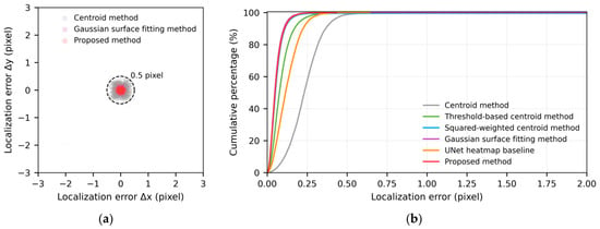
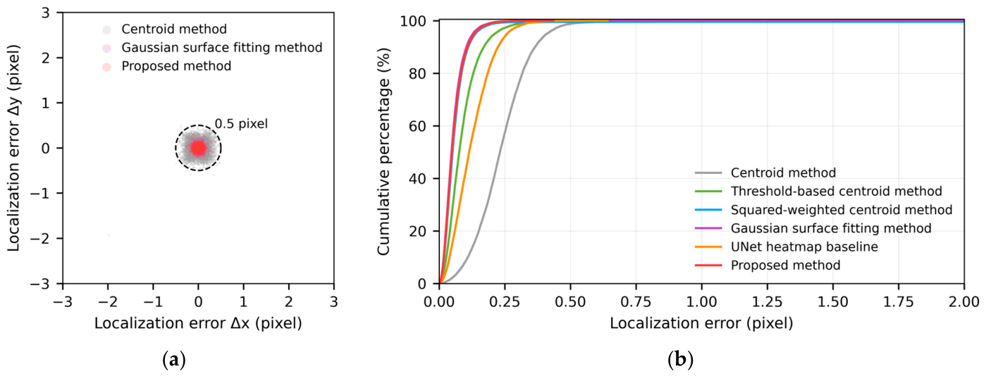
The per-sample error distributions under Setting_C are visualized in Figure 6. The localization errors of the proposed method are tightly concentrated around the origin, whereas those of the centroid method are widely scattered in Figure 6a; its cumulative distribution rises fastest among all methods in Figure 6b. Although the Gaussian surface fitting method also confines most samples within 0.5 pixels, its long-tailed outliers yield a standard deviation an order of magnitude larger than that of the proposed method.

Figure 6. Localization error distribution under Setting_C. (a) Per-sample errors (Δx,Δy) of the proposed method and representative classical methods; the dashed circle denotes the 0.5-pixel subpixel reference. (b) Cumulative distribution functions (CDFs) of the localization errors for all methods.

3.4.3. Ablation Study

To validate each core design component’s contribution to star centroid measurement performance, we conducted ablation studies on the independent test set, which contains 45,000 star maps covering all three operating conditions.

Taking the complete model proposed in this paper as the baseline (denoted as M0), five ablation variants are constructed by sequentially removing or replacing key components:

• M1 removes the subpixel regression branch and directly outputs integer peak coordinates obtained from the probability heatmap via NMS, which is designed to validate the contribution of the geometric quantization compensation mechanism to subpixel localization accuracy;
• M2 removes the physical centroid loss, retaining only the energy-aware heatmap loss and subpixel geometric offset loss during training, aiming to verify the role of the physical centroid loss in suppressing accumulated errors from independent branch predictions;
• M3 replaces the improved focal loss in heatmap supervision with a standard BCE loss averaged over all pixels (i.e., removing focal modulation, asymmetric weighting, and class-wise decoupled normalization), to assess the necessity of the improved loss design under extreme positive-negative sample imbalance;
• M4 replaces the full-resolution feature extraction architecture with a downsampling structure comprising two convolutional layers with stride 2, to validate the contribution of the full-resolution feature preservation design to the retention of spatial detail information.
• M5 replaces the improved focal loss with the standard focal loss (α = 0.25, γ = 2), following the original notation and recommended values of Lin et al. [36], distinct from α and β in Equation (6), with all other settings identical to M0, to directly quantify the gain brought by the improved focal design.

All variants use the same dataset, training strategy, and evaluation metrics as M0 to ensure a fair comparison. The configurations of the variants are summarized in Table 6, the sensitivity of the key hyperparameters is reported in Table 7, and the three-condition ablation results are presented in Table 8.

Table 6. Configurations of the ablation variants.

Variant	Full Resolution Architecture	Subpixel Regression Branch	Physical Centroid Loss	Improved Focal Loss
M0	✓	✓	✓	✓
M1	✓	✗	✓	✓
M2	✓	✓	✗	✓
M3	✓	✓	✓	✗
M4	✗	✓	✓	✓
M5	✓	✓	✓	✗

Note: ✓ denotes that the component is retained; ✗ denotes that the component is removed or replaced. In M3, the improved focal loss is replaced by standard BCE loss; in M5, it is replaced by the standard focal loss (α = 0.25, γ = 2).

Table 7. Hyperparameter sensitivity analysis on the validation set.

Group	Setting	Overall Mean Error (Pixel)	Setting_C Std (Pixel)	Detection Rate (%)
Focal loss (α, β)	(2, 4) *	0.0275	0.0399	100
	(1, 4)	0.0279	0.0399	100
	(3, 4)	0.0275	0.0395	100
	(2, 2)	0.0284	0.0399	100
	(2, 6)	0.0273	0.0396	100
Loss weights (λ1, λ2, λ3)	(1, 0.1, 0.1) *	0.0275	0.0399	100
	(1, 1, 0.1)	0.0274	0.0396	100
	(1, 0.1, 1)	0.0277	0.0402	100
Heatmap label σp	0.3	0.0278	0.0399	100
	0.5 *	0.0275	0.0399	100
	0.8	0.0284	0.0399	100

Note: * Settings adopted in this work. All results are evaluated on the validation set of 45,000 maps.

Table 8. Ablation results under the three operating conditions on the independent test set (mean error in pixels).

Variant	Setting_A	Setting_B	Setting_C	Overall	Detection Rate (%)
M0	0.0096	0.0151	0.0576	0.0274	100
M1	0.3828	0.3834	0.3886	0.3849	100
M2	0.3065	0.3123	0.3261	0.3150	100
M3	-	-	-	-	0
M4	0.0149	0.0240	0.0768	0.0386	100
M5	0.0106	0.0160	0.0592	0.0286	100

Note: M3 fails to yield valid detections when the improved focal loss is replaced with standard BCE loss, resulting in uncomputable accuracy metrics, denoted by -; bolded values indicate the optimal results.

Table 7 summarizes the hyperparameter sensitivity on the validation set. To eliminate any ambiguity regarding test-set independence, all hyperparameter sensitivity experiments are reported on the validation set, and the independent test set is used exclusively for the final performance metrics. Five (α,β) combinations of the improved focal loss yield overall mean errors within 0.0273–0.0284 pixels and Setting_C standard deviations within 0.0395–0.0399 pixels, showing that the performance is insensitive to the focal modulation parameters. Scaling the subpixel offset weight λ₂ or the centroid weight λ₃ from 0.1 to 1.0 changes the overall mean error by no more than 0.0002 pixels, whereas setting λ₃ = 0, equivalent to variant M2 in Table 8, degrades the overall mean error to 0.3150 pixels on the test set, confirming that the physical centroid constraint is the only critically sensitive loss weight. Varying the heatmap label standard deviation σ_p over 0.3, 0.5, and 0.8 keeps the overall mean error within 0.0275–0.0284 pixels.

Statistics collected during the training of M0 show that the proportion of samples discarded by the centroid-loss activation threshold, whose peak heatmap confidence falls below 0.2, is approximately 8.4% in the first epoch and drops to 0% from the second epoch onward, confirming that the activation threshold does not impede the convergence of the network.

Removing the subpixel regression branch (M1) increases the overall mean error from 0.0274 pixels to 0.3849 pixels, and its per-condition errors remain nearly constant at 0.3828–0.3886 pixels, aligning with the theoretical uniform quantization error of integer grid sampling of approximately 0.38 pixels. The branch thus nearly eliminates the quantization truncation error introduced by discrete detector sampling.

Removing the physical centroid loss (M2) increases the overall mean error and standard deviation to approximately 11.5-fold and 8.1-fold those of M0, reaching 0.3150 and 0.2578 pixels, respectively. This shows that the end-to-end geometric constraint on the final decoded coordinates suppresses cumulative errors from independent branch predictions and coordinate-grid quantization.

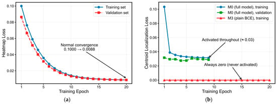
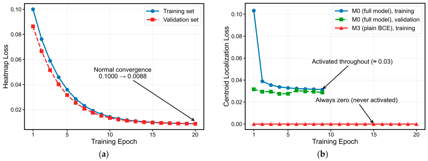
Compared with the full model M0, M3—where the improved focal loss is replaced with standard BCE loss averaged over all image pixels—fails. During training, although the average heatmap loss monotonically converges from 0.100 to 0.0088, the peaks of the predicted heatmaps never exceed the effective response threshold. Consequently, centroid supervision remains inactive throughout training, leading to a final detection rate of 0 on all three operating conditions. This indicates that the network converges to a trivial all-background solution: approximately 99% of background pixels dominate the gradient, completely overwhelming the supervisory signal from star-point positive samples. The class-wise decoupled normalization and focal modulation mechanisms are thus essential for maintaining valid star-point responses under extreme positive-negative sample imbalance (training dynamics are compared in Figure 7).

Figure 7. Training failure mechanism of the M3 variant (standard binary cross-entropy loss). (a) The heatmap loss of M3 converges normally during training; (b) The physical centroid loss remains activated throughout the training process in the full model M0 (approximately 0.03), while it stays at zero (never activated) in M3—eventually leading the network to degenerate into an all-background prediction.

Introducing two-stage downsampling (M4) increases the overall mean error to 0.0386 pixels and the Setting_C standard deviation from 0.0397 to 0.2186 pixels, although its inference time decreases to 0.68 ms. The loss of star-point edge-distribution information occurs at the downsampling stage and cannot be recovered by terminal upsampling. M5 achieves an overall mean error of 0.0286 pixels with a 100% detection rate; the improved focal loss thus yields a gain of 0.0012 pixels (approximately 4.2%) over the standard focal loss. Together with the complete failure of M3, this indicates that focal-type modulation is essential for successful training under the extreme class imbalance of this task, while the improved variant brings a further, consistent but modest gain over the standard focal loss. In summary, the ablation experiments identify the full-resolution architecture, the subpixel regression branch, and the physical centroid loss as the primary accuracy-bearing designs, and focal-type heatmap modulation as a necessary condition for successful training.

4. Discussion

4.1. Comparison with Existing Research

The dual-branch measurement head in this paper inherits the paradigm of center point detection methods in general computer vision [35], both adopting a decoupled design of heatmap localization and offset compensation. However, they differ fundamentally at the physical mechanism level. In generic object detection, the offset branch compensates for coordinate quantization errors introduced by network downsampling strides. In contrast, the subpixel regression branch in this work addresses quantization truncation errors inherent to the detector’s discrete sampling—with its supervision signal directly derived from the physical ground truth of star energy distribution. Moreover, by targeting precise single-star measurement within 28 × 28-pixel small windows, this method eliminates the need for multi-object association or scale variation handling, enabling a full-resolution architecture [30] that concentrates all network capacity on preserving spatial detail. Among recent advances in star-point measurement: Yuan et al. [15] and Karaparambil et al. [16] improved traditional centroid frameworks, but their accuracy remains constrained by manually imposed model assumptions; Ma et al. [28] proposed a multi-task end-to-end network achieving a root-mean-square error (RMSE) of 0.2826 pixels on real-world data; Luo et al. [26] further validated the feasibility of the keypoint detection paradigm for centroid extraction in high-dynamic star sensors. The proposed method achieves an average error of 0.0576 pixels under simulated extreme conditions and an overall average error of 0.0274 pixels across three scenarios. Under the identical dataset and partition protocol, the U-Net heatmap baseline yields an overall average error of 0.1117 pixels, approximately 4.1 times that of the proposed method. The CenterNet-style heatmap–offset baseline yields an overall mean error of 0.1745 pixels, approximately 6.4 times that of the proposed method; together with variants M2 (heatmap + offset without centroid loss) and M4 (downsampling backbone) in Table 8, this confirms that the accuracy gain stems from the physical centroid constraint and the full-resolution architecture rather than from the heatmap paradigm itself.

4.2. Limitations

This study has the following limitations:

(1)

Validation relies on high-fidelity simulated star maps. Although we incorporated optical aberration distortions, radiometric hot-pixel injection, and detector noise models during dataset construction to approximate real-world imaging conditions, domain gaps may persist between simulated data and in-orbit captured images; for example, the dynamic elliptization of star spots induced by optical defocusing is not specifically modeled. Thus, this study’s conclusions warrant further validation using actual on-orbit data.

(2)

This study focuses on the centroid measurement of single star points within 28 × 28-pixel windows. Extracting star points from full-sky star maps, which requires integration with a front-end object detection module, falls outside the scope of the present work. When multiple stars are adjacent within one window or a star spot is partially truncated at the window boundary, the heatmap response may be biased; in a complete pipeline, such cases are expected to be handled by the front-end extraction module, and they will be investigated together with full-frame processing in future work.

(3)

The timing evaluation was conducted on a ground-based GPU platform. For practical on-orbit deployment, the model still requires quantization, porting, and empirical validation on spaceborne devices (e.g., FPGAs or radiation-hardened SoCs), which is part of our subsequent research plan.

4.3. Engineering Applicability

From an engineering standpoint, the proposed network has approximately 556,000 parameters and a single-frame computational complexity of about 0.87 GFLOPs. Its architecture uses standard convolutions, batch normalization, and residual connections, with no iterative optimization or dynamic control flow. Per-frame inference latency averages 1.07 ms on the tested NVIDIA RTX 4090 platform, with a narrowly concentrated distribution, accounting for only about 1% of the typical sampling period of star sensors and thus meeting the real-time constraint imposed by the fixed sampling interval. Additionally, as a purely static forward graph, the network features a constant computational load with no data-dependent iterations, facilitating pipeline deployment and quantization acceleration on spaceborne programmable devices such as FPGAs. In contrast, iterative methods like Gaussian surface fitting exhibit a significant increase in latency and noticeable jitter under hot-spot interference. By comprehensively evaluating the three metrics of measurement accuracy, robustness, and computational predictability, the proposed method represents a promising candidate for the centroid measurement scheme of next-generation high-precision star sensors, pending validation with real on-orbit data.

5. Conclusions

To address the challenge of balancing accuracy and robustness in star centroid measurement under complex space-borne degradation conditions, this paper proposes a high-precision and robust star centroid measurement method based on probability heatmaps and a subpixel regression network. A full-resolution architecture retains the complete spatial distribution of stellar diffraction spots; the orthogonal decoupling of an energy-distribution-aware heatmap branch and a subpixel regression branch decomposes the non-convex localization problem into regional energy perception and local geometric compensation; and the physical centroid loss directly constrains the final decoded coordinates. The method performs centroid estimation on 28 × 28-pixel star windows after coarse star extraction, while full-sky star extraction and star identification are beyond the scope of this work.

Experiments on an independent test set of 45,000 simulated star maps show a 100% detection rate under ideal, typical, and extreme conditions, with a mean error of 0.0096 pixels under ideal conditions and a standard deviation of 0.0397 pixels under extreme conditions, about 1/12 that of the Gaussian surface fitting method. Ablation experiments identify the full-resolution architecture, the subpixel regression branch, and the physical centroid constraint as the primary sources of localization accuracy, and focal-type heatmap modulation as necessary to prevent collapse into an all-background solution under extreme class imbalance. The network achieves a mean single-frame inference latency of 1.07 ms on the tested NVIDIA RTX 4090 platform, with 99.989% of frames completing within 2 ms and without the data-dependent latency growth of iterative algorithms, meeting the real-time requirement imposed by the fixed sampling period of star sensors, as demonstrated on simulated star maps.

Future work will proceed in three directions. First, transfer validation and fine-tuning will be conducted on real on-orbit star maps to narrow the simulation-to-real domain gap discussed in Section 4.2. Second, joint-solving strategies for scenarios with coexisting or overlapping stars will be investigated to extend the method to complete star-map frames. Third, model lightweighting and deployment on spaceborne embedded platforms will be studied to advance the engineering application of the method.

The proposed method is expected to enhance the attitude measurement accuracy of star sensors onboard Earth-observation satellites, thereby contributing to the geometric fidelity of remote sensing products.

References

- Liebe, C.C. Star trackers for attitude determination. IEEE Aerosp. Electron. Syst. Mag. 1995, 10, 10–16. [Google Scholar] [CrossRef] [Scilit]
- Liebe, C.C. Accuracy performance of star trackers—A tutorial. IEEE Trans. Aerosp. Electron. Syst. 2002, 38, 587–599. [Google Scholar] [CrossRef] [Scilit]
- Wang, X.; Chen, X.; Li, Z.; Zhu, J. An optical system of star sensors with accuracy performance varying with the field of view. Sensors 2023, 23, 8663. [Google Scholar] [CrossRef] [Scilit]
- Chen, D.; Li, X.; Wang, X. Centroid-preserving dynamic star image deblurring for remote sensing satellite attitude measurement via physics-guided bi-level optimization. Remote Sens. 2026, 18, 2610. [Google Scholar] [CrossRef] [Scilit]
- Sulaiman, N.N.; Hasbullah, N.F.; Saidin, N.; Javed, Y.; Khan, Z.I. Radiation-induced degradation in optoelectronic devices for satellite applications: A review. Discov. Mater. 2025, 5, 59. [Google Scholar] [CrossRef] [Scilit]
- Luo, Z.; Feng, J.; Guo, Q.; Li, Y. Centroid localization of dynamic star sensors under proton irradiation. Opt. Precis. Eng. 2025, 33, 2089–2107. (In Chinese) [Google Scholar] [CrossRef] [Scilit]
- Alexander, B.F.; Ng, K.C. Elimination of systematic error in subpixel accuracy centroid estimation. Opt. Eng. 1991, 30, 1320–1331. [Google Scholar] [CrossRef] [Scilit]
- Rufino, G.; Accardo, D. Enhancement of the centroiding algorithm for star tracker measure refinement. Acta Astronaut. 2003, 53, 135–147. [Google Scholar] [CrossRef] [Scilit]
- Mu, S.; Wang, L.; Li, G. A method of star spot center-of-mass localization algorithm for star sensor under highly dynamic conditions. IEEE Sens. J. 2023, 23, 14957–14966. [Google Scholar] [CrossRef] [Scilit]
- Ma, J.; Zhang, S.; Yang, X.; Li, G. A centroid locating method for star sensor based on improved Gaussian surface fitting. In Proceedings of the 15th International Conference on Digital Image Processing (ICDIP), Nanjing, China, 19–22 May 2023; pp. 1–6. [Google Scholar]
- Delabie, T.; De Schutter, J.; Vandenbussche, B. An accurate and efficient Gaussian fit centroiding algorithm for star trackers. J. Astronaut. Sci. 2014, 61, 60–84. [Google Scholar] [CrossRef] [Scilit]
- Wan, X.; Wang, Y.; Wang, G.; Wei, X.; Wang, W.; Li, J.; Zhang, G. A spatial–temporal star spots extraction for high dynamics star sensors. IEEE Sens. J. 2023, 23, 13060–13071. [Google Scholar] [CrossRef] [Scilit]
- Li, T.; Zhang, C.; Kong, L.; Wang, J.; Pang, Y.; Li, H.; Wu, J.; Yang, Y.; Tian, L. Centroiding error compensation of star sensor images for hypersonic navigation based on angular distance. IEEE Trans. Instrum. Meas. 2024, 73, 8508211. [Google Scholar] [CrossRef] [Scilit]
- Yi, J.; Ma, Y.; Long, H.; Lu, K.; Zhao, R. On-orbit high-precision calibration for deep-coupled parameters of star sensor and gyroscope systems. Opt. Express 2024, 32, 32187–32209. [Google Scholar] [CrossRef] [Scilit]
- Yuan, J.; Wu, J.; Kang, G. High-precision centroid localization algorithm for star sensor under strong straylight condition. Remote Sens. 2025, 17, 1108. [Google Scholar] [CrossRef] [Scilit]
- Karaparambil, V.C.; Manjarekar, N.S.; Singru, P.M. Sieve search centroiding algorithm for star sensors. Sensors 2023, 23, 3222. [Google Scholar] [CrossRef] [Scilit]
- Lin, B.; Wu, P.; Wang, H.; Xu, X.; Yang, X.; Zhang, X. A centroiding method for targets in star images based on local PSF estimation and iterative deconvolution. IEEE Trans. Instrum. Meas. 2024, 73, 7009813. [Google Scholar] [CrossRef] [Scilit]
- Zhang, L.; Sun, B.; Liu, H.; Fan, G. Fusion of a priori information and energy distribution for the centroiding method of the star sensor. AIP Adv. 2024, 14, 045045. [Google Scholar] [CrossRef] [Scilit]
- Mu, S.; Wang, L.; Wang, C.; Yu, X.; Wang, Y. Accelerated motion star spot centroid localization method for star tracker under high dynamic conditions. Opt. Express 2025, 33, 52000–52018. [Google Scholar] [CrossRef] [Scilit]
- Tang, X.; Cao, Q.; Fu, Z.; Xu, T.; Duan, R.; Yang, X. Multi-centroid extraction method for high-dynamic star sensors based on projection distribution of star trail. Remote Sens. 2025, 17, 266. [Google Scholar] [CrossRef] [Scilit]
- Xue, D.; Sun, J.; Hu, Y.; Zheng, Y.; Zhu, Y.; Zhang, Y. StarNet: Convolutional neural network for dim small target extraction in star image. In Proceedings of the 2018 IEEE Fourth International Conference on Multimedia Big Data (BigMM), Xi’an, China, 13–16 September 2018; pp. 1–7. [Google Scholar] [CrossRef] [Scilit]
- Mastrofini, M.; Agostinelli, I.; Curti, F. Design and validation of a U-Net-based algorithm for star sensor image segmentation. Appl. Sci. 2023, 13, 1947. [Google Scholar] [CrossRef] [Scilit]
- Zapevalin, P.R.; Novoselov, A.; Zharov, V.E. Artificial neural network for star tracker centroid computation. Adv. Space Res. 2023, 71, 3917–3925. [Google Scholar] [CrossRef] [Scilit]
- Zhao, H.; Lembeck, M.F.; Zhuang, A.; Shah, R.; Wei, J. Real-time convolutional neural network-based star detection and centroiding method for CubeSat star tracker. IEEE Trans. Aerosp. Electron. Syst. 2025, 61, 8172–8184. [Google Scholar] [CrossRef] [Scilit]
- Liu, H.; Wei, X.; Wang, G.; Li, J. A star spot extraction method based on SSA-UNet for star sensors under dynamic conditions. IEEE Sens. J. 2023, 23, 7410–7419. [Google Scholar] [CrossRef] [Scilit]
- Luo, Z.; Guo, Q.; Feng, J.; Li, Y.; Zhang, X. Centroid algorithm for high-dynamic star sensor based on key point detection deep learning algorithms. Opt. Express 2025, 33, 17203–17232. [Google Scholar] [CrossRef] [Scilit]
- Chen, X.; Yan, H.; Ding, G.; He, Y.; Zhang, M. On-orbit correction method for star sensor imaging based on deep neural network. Chin. Opt. 2024, 17, 71–82. [Google Scholar]
- Ma, R.; Ding, G.; Han, S.; Li, Z.; Bi, Z.; Zhu, Z.; Yan, H. End-to-end subpixel positioning method for space dim and weak point targets based on multi-task learning. Opt. Commun. 2025, 596, 132370. [Google Scholar] [CrossRef] [Scilit]
- Ronneberger, O.; Fischer, P.; Brox, T. U-Net: Convolutional networks for biomedical image segmentation. In Proceedings of the Medical Image Computing and Computer-Assisted Intervention (MICCAI), Munich, Germany, 5–9 October 2015; pp. 234–241. [Google Scholar] [CrossRef] [Scilit]
- Sun, K.; Xiao, B.; Liu, D.; Wang, J. Deep high-resolution representation learning for human pose estimation. In Proceedings of the IEEE/CVF Conference on Computer Vision and Pattern Recognition (CVPR), Long Beach, CA, USA, 15–20 June 2019; pp. 5693–5703. [Google Scholar] [CrossRef] [Scilit]
- He, K.; Zhang, X.; Ren, S.; Sun, J. Deep residual learning for image recognition. In Proceedings of the IEEE Conference on Computer Vision and Pattern Recognition (CVPR), Las Vegas, NV, USA, 27–30 June 2016; pp. 770–778. [Google Scholar] [CrossRef] [Scilit]
- Ioffe, S.; Szegedy, C. Batch normalization: Accelerating deep network training by reducing internal covariate shift. In Proceedings of the 32nd International Conference on Machine Learning (ICML), Lille, France, 6–11 July 2015; pp. 448–456. [Google Scholar]
- Srivastava, N.; Hinton, G.; Krizhevsky, A.; Sutskever, I.; Salakhutdinov, R. Dropout: A simple way to prevent neural networks from overfitting. J. Mach. Learn. Res. 2014, 15, 1929–1958. [Google Scholar]
- Law, H.; Deng, J. CornerNet: Detecting objects as paired keypoints. Int. J. Comput. Vis. 2020, 128, 642–656. [Google Scholar] [CrossRef] [Scilit]
- Zhou, X.; Wang, D.; Krähenbühl, P. Objects as points. arXiv 2019, arXiv:1904.07850. [Google Scholar]
- Lin, T.-Y.; Goyal, P.; Girshick, R.; He, K.; Dollár, P. Focal loss for dense object detection. In Proceedings of the IEEE International Conference on Computer Vision (ICCV), Venice, Italy, 22–29 October 2017; pp. 2980–2988. [Google Scholar] [CrossRef] [Scilit]
- Girshick, R. Fast R-CNN. In Proceedings of the IEEE International Conference on Computer Vision (ICCV), Santiago, Chile, 7–13 December 2015; pp. 1440–1448. [Google Scholar] [CrossRef] [Scilit]
- Pan, D.; Zhou, Q.; Liu, X.; Liu, B.; Fang, H. Modeling and detection of star spot in high dynamic condition. Acta Photonica Sin. 2022, 51, 0304002. [Google Scholar]
- Paszke, A.; Gross, S.; Massa, F.; Lerer, A.; Bradbury, J.; Chanan, G.; Killeen, T.; Lin, Z.; Gimelshein, N.; Antiga, L.; et al. PyTorch: An imperative style, high-performance deep learning library. In Proceedings of the 33rd Conference on Neural Information Processing Systems (NeurIPS), Vancouver, BC, Canada, 8–14 December 2019. [Google Scholar]
- Loshchilov, I.; Hutter, F. Decoupled weight decay regularization. In Proceedings of the 7th International Conference on Learning Representations (ICLR), New Orleans, LA, USA, 6–9 May 2019. [Google Scholar]
Disclaimer/Publisher’s Note: The statements, opinions and data contained in all publications are solely those of the individual author(s) and contributor(s) and not of MDPI and/or the editor(s). MDPI and/or the editor(s) disclaim responsibility for any injury to people or property resulting from any ideas, methods, instructions or products referred to in the content. |
© 2026 by the authors. Licensee MDPI, Basel, Switzerland. This article is an open access article distributed under the terms and conditions of the Creative Commons Attribution (CC BY) license.