


Abstract
Procedural fractals provide reproducible multi-scale structures that can serve as controlled targets for evaluating resolution-dependent changes introduced during rasterization. This study investigated the effects of rasterization resolution on geometric, spectral, high-frequency, and structural image properties using fifteen procedurally generated PostScript fractals rasterized at 150, 300, 600, and 1200 DPI, with 1200 DPI used as an operational high-resolution reference. Rasterization fidelity was quantified using fractal-dimension deviation (ΔD), power spectral density slope deviation (Δβ), high-frequency energy ratio (EHF), and multi-scale averaged structural similarity (QMS). Increasing resolution significantly reduced ΔD and Δβ (p < 0.001), while EHF decreased systematically across all four resolutions (p < 0.001). QMS was already high at 150 DPI (0.9667 ± 0.0188) and increased to 0.9931 ± 0.0058 at 600 DPI (p < 0.001). Expected monotonic trajectories were observed for 12/15 fractals for ΔD, 14/15 for Δβ, and 15/15 for both EHF and QMS. These findings show that high structural similarity can coexist with measurable resolution-dependent differences in scale-sensitive geometric and spectral properties, supporting procedural fractals as reproducible candidate multi-scale targets for evaluating rasterization fidelity.
1. Introduction
Digital images are rarely direct representations of visual scenes; instead, they result from a sequence of physical and computational processes that transform scene information into discrete pixel-based representations. Computational imaging integrates image formation, sampling, and computational processing within a unified framework [1,2]. More recently, the concept of computational image formation has further emphasized the role of numerical forward models and controlled simulation in understanding and reproducing image-formation processes [3]. As modern imaging systems increasingly rely on software-defined transformations, understanding how individual computational operations influence the structural properties of the resulting images has become an important aspect of quantitative imaging-system evaluation.
Rasterization, the conversion of resolution-independent graphical descriptions into discrete raster representations—is a fundamental operation in visualization, digital publishing, display rendering, and computer graphics. Although rasterization is often regarded as a technical conversion step, it necessarily involves spatial sampling. According to classical sampling theory, insufficient sampling density limits the accurate representation of high spatial frequencies and may introduce aliasing and other resolution-dependent distortions [4,5]. Consequently, rasterization resolution may affect local geometry, spatial-frequency distributions, and the structural fidelity of the resulting image. These effects are particularly relevant when quantitative image measurements depend on preserving fine structural information across multiple spatial scales.
Conventional imaging-system evaluation commonly relies on standardized targets designed to characterize properties such as spatial resolution and spatial-frequency response, including those specified in ISO 12233:2024 [6]. Controlled resolution targets remain widely used for objective characterization of contemporary imaging systems; for example, recent work has employed resolution targets together with modulation-transfer-function analysis to quantitatively evaluate image quality in digital acquisition systems [7]. Such targets provide well-established measurements of imaging-system performance but primarily consist of predefined edges, lines, wedges, or periodic structures. They are therefore not specifically designed to represent deterministic structural complexity distributed continuously across a broad range of spatial scales.
Fractal geometry provides a mathematical framework for describing structures that exhibit scale-dependent complexity and self-similar organization [8,9]. Unlike conventional resolution targets, procedurally generated fractal structures can contain geometric information across multiple spatial scales while remaining deterministic and reproducible. These characteristics make fractal patterns attractive candidates for controlled synthetic targets in studies of sampling and resolution-dependent image formation.
At the same time, estimation of fractal properties from digital images presents specific methodological challenges. The fractal dimension (FD) obtained from a raster representation is affected by finite spatial resolution, the available scaling interval, pixel quantization, and the numerical implementation of the estimator. Early systematic investigations demonstrated that sampling resolution and quantization can substantially influence FD estimates obtained from digital images [10], while subsequent studies showed that downscaling pixel resolution affects the estimated generalized dimensions of both mathematically defined and experimentally observed fractals [11]. The selection of an appropriate range of box sizes and spatial scales is likewise critical for reliable box-counting estimation [12,13].
These methodological issues remain active areas of research. Recent approaches have proposed improved image-based fractal-dimension estimators [14], accelerated box-counting implementations for multidimensional digital data [15], and computational frameworks specifically designed to reduce quantization and box-selection errors in fractal analysis of optical images [16]. Datseris et al. provided a comparative assessment of contemporary numerical fractal-dimension estimators and highlighted the influence of finite data, estimator selection, and implementation choices on the resulting measurements [17]. More recently, D’Orazio et al. explicitly investigated the influence of image resolution on box-counting fractal-dimension estimates using both mathematically defined fractals and experimentally acquired images, demonstrating deterioration in estimation accuracy as the available spatial resolution is reduced [18]. Automated optimization of scaling regions and grid placement has also been proposed to reduce discretization and boundary-related bias in box-counting analysis [19]. Together, these studies demonstrate that raster resolution is not merely a presentation parameter but can directly influence quantitative measurements of multi-scale image structure.
Image preprocessing represents an additional consideration when fractal dimension is estimated from extracted structural boundaries rather than directly from the original intensity representation. In edge-based approaches, the detected contour itself becomes the input to subsequent geometric analysis. The Canny edge detector remains a widely used method because it combines gradient estimation, non-maximum suppression, and hysteresis thresholding within a systematic edge-detection framework [20]. However, the resulting edge representation depends on detector parametrization, particularly threshold selection. Recent work has therefore continued to investigate adaptive threshold-selection strategies for Canny edge detection [21,22]. When such edge representations constitute the input to subsequent geometric measurements such as box-counting FD, consistent preprocessing across experimental conditions is essential.
Frequency-domain analysis provides complementary information about resolution-dependent structural changes. Spatial sampling determines the frequency range that can be represented without ambiguity, while insufficient sampling may attenuate, redistribute, or alias fine-scale frequency components. Power spectral density (PSD) analysis therefore provides a means of characterizing the distribution of image energy across spatial frequencies. Recent investigations have demonstrated that PSD-derived descriptors can be sensitive to sampling interval and spatial resolution [23]. For fractal and approximately scale-invariant structures, spectral analysis is particularly relevant because their spatial organization extends over multiple scales. Combining geometric fractal measures with spectral descriptors therefore provides complementary information regarding preservation of multi-scale structure after rasterization.
Structural image-quality measures provide a further complementary perspective. The Structural Similarity Index (SSIM) was introduced as an alternative to purely pixel-error-based quality measures by evaluating local luminance, contrast, and structural relationships [24], while its multi-scale extension incorporates structural comparisons across multiple image scales [25]. Contemporary image-quality research continues to emphasize that objective quality assessment requires metrics capable of representing structural and perceptually meaningful changes rather than relying solely on pixel-level errors [26]. This consideration is particularly relevant when rasterized representations generated at different spatial sampling densities must be compared after spatial alignment or resampling.
Natural images are widely used in image-quality evaluation, but they have limitations when the goal is to isolate the effect of a specific image-formation operation. Their structural and statistical properties are inherently complex, the underlying continuous scene representation is generally unavailable, and separating processing-induced changes from intrinsic scene variability can therefore be difficult. Synthetic and computationally generated images offer an alternative because their generation processes can be explicitly controlled. Research on synthesized-image quality has also shown that distortions in computationally generated imagery are often strongly associated with local structural and high-frequency information, motivating evaluation strategies that combine structural and frequency-domain information [27].
Procedurally defined fractal scenes provide a particularly useful form of controlled synthetic imagery for this purpose. A procedural program can preserve the same underlying graphical definition while allowing rasterization parameters to be varied independently. This enables the effects of spatial sampling to be studied without simultaneously changing scene content. PostScript is especially suitable for such experiments because its graphical descriptions are resolution-independent and are converted into discrete pixel representations only during rasterization.
Despite extensive research on fractal-dimension estimation, finite-resolution effects, edge extraction, spectral analysis, and image-quality assessment, these topics have largely been investigated separately. Previous studies have mainly examined how resolution influences the measurement of fractal properties, how sampling affects spectral descriptors, or how image-processing operations affect structural quality. Considerably less attention has been given to the complementary perspective of using procedurally defined fractal structures as controlled multi-scale targets for quantitatively characterizing the rasterization process itself through geometric, spectral, high-frequency-energy, and structural measures within a unified experimental framework.
In this work, procedurally generated PostScript fractals are investigated as controlled multi-scale test targets for rasterization analysis within a computational imaging framework. A dataset of fifteen distinct procedural fractal programs was rasterized using Ghostscript at multiple spatial sampling densities. Because the procedural scene description remains unchanged across rasterization conditions, the resulting dataset provides a controlled environment in which rasterization resolution is the principal experimentally varied image-formation parameter.
To evaluate resolution-dependent structural fidelity, a multi-domain analysis framework combining four complementary measures is employed. Fractal-dimension deviation quantifies changes in estimated geometric complexity; power spectral density slope deviation characterizes changes in frequency scaling; a high-frequency energy ratio describes resolution-dependent changes in relative high-frequency spectral content; and a multi-scale averaged SSIM measure evaluates structural similarity relative to a high-resolution reference. Joint analysis of these descriptors enables rasterization to be examined as a scale-dependent image-formation operation rather than solely as a technical vector-to-raster conversion.
The main contributions of this work are threefold. First, procedurally defined fractal scenes are investigated as reproducible multi-scale evaluation targets for quantitative rasterization analysis. Second, a unified framework combining geometric, spectral, high-frequency-energy, and structural measures is applied to characterize resolution-dependent rasterization effects. Third, the consistency of these effects is evaluated across fifteen structurally distinct procedural fractals, providing evidence for the potential of controlled fractal scenes as reproducible test targets for studies of raster image formation.
2. Materials and Methods
2.1. Procedural Fractal Dataset
The experimental dataset consists of fifteen procedurally generated fractal images defined as independent PostScript programs. Each program describes a deterministic generative process composed of iterative geometric transformations, stochastic coordinate generation, and repeated path construction operations. The fractals were designed to exhibit complex spatial organization and multi-scale structural characteristics while remaining fully reproducible through fixed pseudo-random initialization.
The complete set of fifteen procedural fractals used in the study is shown in Figure 1. The examples displayed correspond to the 150 DPI rasterizations. The test set includes diverse geometric arrangements and spatial structures, providing a range of multi-scale patterns for evaluating resolution-dependent changes introduced during rasterization.
Figure 1.
Procedural fractal test images used in the study.
Unlike raster images, PostScript descriptions represent images as resolution-independent vector procedures. Consequently, the underlying geometric structure remains unchanged regardless of output resolution, making these fractals suitable as controlled test targets for studying rasterization effects. Each fractal instance differs in transformation parameters, iteration counts, and geometric construction rules, providing structural diversity across the dataset. This structural diversity was also reflected quantitatively in the raster-derived descriptors. Across the fifteen designs, the estimated fractal dimension D ranged from 1.4491 to 1.6583 at 150 DPI and from 1.3854 to 1.6490 at 1200 DPI, while the PSD slope β ranged from 2.1353 to 2.6231 and from 2.2858 to 2.7959, respectively. The high-frequency energy ratio also varied substantially among designs, ranging from 0.0069 to 0.0653 at 150 DPI and from 0.0009 to 0.0319 at 1200 DPI. These ranges confirm that the test set encompasses quantitatively distinct geometric and spectral characteristics rather than repeated instances of a single structural configuration. Figure 2 shows a representative procedural fractal rendered at the four rasterization resolutions used throughout this study.
Figure 2.
Representative procedural fractal rasterized at four spatial resolutions: (a) 150 DPI, (b) 300 DPI, (c) 600 DPI, and (d) 1200 DPI. Black squares indicate the regions selected for detailed comparison.
All programs were executed using identical rendering conditions except for the rasterization parameters varied during the experiments.
2.2. Rasterization Pipeline
The PostScript fractals were rasterized through the GSview 5.0 File → Convert interface using Ghostscript 10.06.0 with the png16m output device at 150, 300, 600, and 1200 DPI. No additional device properties or command-line options were manually specified in the GSview conversion dialog; thus, rendering other than the selected rasterization resolution followed the default settings of the installed GSview/Ghostscript configuration. The same conversion procedure and device settings were maintained for all fractals and all rasterization resolutions.
Each fractal program was rasterized at four spatial sampling densities:150, 300, 600 and 1200 DPI.
The resulting raster dimensions were 1275 × 1650 pixels at 150 DPI, 2550 × 3300 pixels at 300 DPI, 5100 × 6600 pixels at 600 DPI, and 10,200 × 13,200 pixels at 1200 DPI, corresponding to the expected 1:2:4:8 sampling relationship while preserving the same physical field of view.
The highest resolution (1200 DPI) served as the reference representation for subsequent comparative analysis. Output images were exported using the png16m device to ensure lossless 24-bit RGB encoding without compression artifacts.
All images were rendered using the same GSview/Ghostscript conversion procedure and the same png16m output device. No additional rendering options were manually changed between conversions; rasterization resolution was the experimentally varied parameter.
To illustrate how rasterization resolution affects local structural detail, enlarged views of the marked regions are presented in Figure 3. All inset images are displayed at identical magnification to enable direct visual comparison.
Figure 3.
Enlarged (5×) views of the regions indicated in Figure 2. Panels correspond to (a) 150 DPI, (b) 300 DPI, (c) 600 DPI, and (d) 1200 DPI. All zoomed views are shown at the same magnification.
2.3. Image Preprocessing
Generated raster images were converted from RGB to grayscale intensity representations prior to quantitative analysis. Grayscale conversion was performed using the luminance transformation
where R, G and B denote the red, green, and blue image channels, respectively. For each image, grayscale intensities were linearly normalized to the range [0, 1] for subsequent numerical analysis.
I = 0.2126R + 0.7152G + 0.0722B,
No filtering, denoising, histogram equalization, sharpening, or other image-enhancement operations were applied. Identical preprocessing parameters were used for all fifteen fractals and all four rasterization resolutions to maintain a fixed analysis pipeline.
For fractal-dimension, power-spectral-density, and high-frequency-energy analyses, each rasterization was evaluated at its native pixel dimensions without geometric resampling. Consequently, these measurements characterize the raster representations produced directly at the corresponding rasterization resolutions.
Structural-similarity analysis required images with corresponding spatial dimensions. For the multi-scale averaged SSIM (QMS) analysis, the complete 1200 DPI reference rasterization was therefore downsampled to the pixel dimensions of the corresponding lower-resolution test image using area-based interpolation (cv2.INTER_AREA). No center cropping was applied, thereby preserving the complete field of view of both representations. The resulting aligned image pair was subsequently used for the multi-scale structural-similarity analysis described in Section 2.4.4.
Although the underlying PostScript descriptions are resolution-independent, the four quantities used in the present study are defined or measured on discrete raster representations. Fractal dimension was estimated from raster-derived edge maps, the PSD slope and high-frequency energy ratio were obtained from the discrete Fourier spectrum, and QMS requires spatially corresponding raster image pairs. Therefore, directly corresponding vector-domain values are not available for all four metrics within the present analysis framework.
The 1200 DPI rasterization served as the operational high-resolution reference for comparative metrics. Accordingly, lower-resolution measurements were interpreted relative to the corresponding 1200 DPI representation generated from the same procedural PostScript fractal. The reference rasterization was not assumed to be an error-free ground truth, but rather a consistent high-resolution baseline within the investigated range of rasterization resolutions.
2.4. Multi-Domain Structural Analysis
To capture different aspects of rasterization-induced changes, four complementary quantitative measures were employed.
2.4.1. Fractal Dimension Analysis
Fractal dimension (FD) was used to quantify the geometric complexity and scale-invariant characteristics of the rasterized fractal images. Unlike conventional geometric descriptors, the fractal dimension measures structural complexity across multiple spatial scales, making it particularly suitable for evaluating self-similar procedural fractals. Because rasterization modifies local edge geometry through finite spatial sampling, changes in fractal dimension provide an indirect measure of structural fidelity.
Before fractal analysis, all raster images were converted from RGB to grayscale and normalized to the intensity range [0, 1]. No additional filtering, denoising, contrast enhancement, or histogram equalization was applied. The preprocessing and edge-detection procedures were held constant across rasterization resolutions, allowing resolution-dependent differences in fractal-dimension estimates to be evaluated under a fixed analysis pipeline. For Canny edge detection, the normalized grayscale image was converted to an 8-bit representation on the range 0–255. Binary edge maps were then extracted using the OpenCV Canny implementation with fixed lower and upper thresholds of 50 and 150, respectively [20]. Identical parameters were used for every rasterization resolution, ensuring that edge extraction remained consistent throughout the dataset. The resulting binary edge maps served as input for fractal-dimension estimation.
The fractal dimension was estimated using the classical box-counting method, one of the most widely used techniques for characterizing self-similar image structures [10,12,17,28]. A sequence of square grids with progressively decreasing box size ε was superimposed on the binary edge image. For each grid size, the number of occupied boxes, denoted by N(ε), was determined. The fractal dimension corresponds to the scaling exponent relating the number of occupied boxes to the box size and is defined as
In practice, this limit cannot be evaluated directly for digital images because only a finite range of spatial scales is available. Therefore, the fractal dimension was estimated from the slope of a least-squares linear regression performed in the logarithmic domain using multiple box sizes distributed approximately uniformly on a logarithmic scale [12,17,19,28]. This implementation provides a robust estimate of the scaling behavior while reducing the influence of discretization effects occurring at very small and very large box sizes.
The goodness of the linear fit was quantified using the coefficient of determination (R2). This diagnostic was calculated for each fractal design and rasterization resolution to assess the goodness of the linear approximation in the log–log relationship used for estimating D.
To quantify rasterization-induced geometric degradation, the deviation of the fractal dimension from the reference image was calculated as
where Dr denotes the fractal dimension measured at rasterization resolution r, and Dref represents the fractal dimension obtained from the 1200 DPI rasterization, which was selected as the reference representation throughout this study.
ΔD = ∣Dr − Dref∣,
Consequently, the reference image satisfies
by definition. Analogously, the corresponding spectral deviation satisfies ∆β = 0, while the multiscale averaged similarity measure satisfies QMS = 1 for the reference image by definition.
∆D = 0
Smaller values of ∆D therefore indicate closer agreement of the estimated fractal dimension with the operational 1200 DPI reference. Because the fractal dimension characterizes scale-dependent structural organization rather than local pixel differences, this metric complements spectral and structural image-quality measures.
Although box-counting is widely used for estimating image fractal dimension, its accuracy depends on the available range of spatial scales and the quality of the extracted edge representation. To minimize methodological bias, identical preprocessing, edge-detection parameters, and box-size sequences were used for every rasterization resolution and for all fifteen procedural fractals. This ensured methodological consistency across all rasterization resolutions and allowed resolution-dependent differences in fractal-dimension estimates to be evaluated under a fixed analysis pipeline.
2.4.2. Power Spectral Density (PSD) Slope
While the fractal dimension quantifies the preservation of geometric complexity in the spatial domain, spectral analysis provides complementary information about the distribution of image energy across spatial frequencies. Rasterization modifies the frequency content of an image through discrete spatial sampling, leading to attenuation or distortion of high-frequency components. Consequently, analysis of the power spectral density (PSD) enables quantitative assessment of the extent to which the scale-dependent frequency characteristics of procedural fractals are preserved after rasterization [23].
Before Fourier transformation, the mean grayscale intensity of each image was subtracted to suppress the dominant DC contribution. For each grayscale raster image, the two-dimensional discrete Fourier transform (2D-DFT) was computed using the Fast Fourier Transform (FFT). The zero-frequency component was shifted to the center of the spectrum before analysis, and the power spectrum was calculated as
where F(u,v) denotes the complex Fourier transform of the image and P(u,v) represents the corresponding spectral power at spatial frequency coordinates (u,v).
P(u,v) = ∣F(u,v)∣2
To obtain a one-dimensional summary of the two-dimensional power spectrum, radial averaging was applied over spectral components at equal radial distance from the center of the shifted Fourier spectrum. The radial spatial frequency was defined as
where (u0, v0) denotes the center of the shifted Fourier spectrum. The spectral power was then averaged over spectral components sharing the same radial distance from the spectrum center. This procedure reduces directional bias while preserving the overall frequency-scaling behavior [23].
Fractal-like image structures exhibit an approximate power-law relationship between spectral power and spatial frequency [29],
where β denotes the spectral scaling exponent. The exponent was estimated from a least-squares linear regression performed in logarithmic coordinates,
where c is a constant representing the intercept of the fitted regression line. The PSD-slope regression was performed over radial bins from bin 5 to min (cy, cx) − 1, where cy and cx denote the center coordinates of the shifted Fourier spectrum. This interval excluded the DC-dominated low-frequency region and radial bins outside the selected fitting range.
P(r)∝r−β,
logP(r) = −βlogr + c,
The goodness of the log–log linear fit used to estimate β was likewise quantified using the coefficient of determination (R2) for each fractal design and rasterization resolution.
To quantify spectral degradation introduced by rasterization, the deviation of the PSD slope from the reference image was computed as
where βr denotes the PSD slope measured at rasterization resolution r, and βref corresponds to the 1200 DPI reference rasterization.
Δβ = ∣βr − βref∣,
Accordingly,
for the reference image by definition, since all spectral comparisons were performed relative to the highest rasterization resolution.
∆β = 0
Lower values of ∆β indicate closer agreement of the estimated spectral scaling behavior with the operational 1200 DPI reference. Unlike conventional resolution metrics that evaluate only local edge sharpness, the PSD slope characterizes the global distribution of spatial frequencies over multiple scales, providing a complementary measure of rasterization quality that is less dependent on isolated local image features.
Because the PSD slope is estimated from the entire image spectrum rather than from isolated image features, it is relatively robust to local edge irregularities while remaining sensitive to systematic changes in spatial sampling. The use of an identical Fourier-processing pipeline, radial averaging procedure, and regression method for every rasterization resolution ensured methodological consistency, allowing resolution-dependent differences in Δβ to be evaluated under a fixed analysis pipeline.
2.4.3. High-Frequency Energy Ratio
To complement the PSD-slope analysis, the relative amount of spectral energy contained in the high-frequency region was quantified using the high-frequency energy ratio (EHF). Whereas ∆β characterizes changes in the overall spectral scaling behavior, EHF measures the proportion of image energy contained within a predefined high-frequency region. This distinction is particularly relevant for procedural fractals, which contain structural information over a broad range of spatial scales and are therefore sensitive to changes introduced by finite raster sampling.
For each grayscale image, the two-dimensional discrete Fourier transform was computed using the Fast Fourier Transform (FFT), and the zero-frequency component was shifted to the center of the spectrum. The corresponding two-dimensional power spectrum was calculated as follows [23]:
where F(u,v) denotes the complex Fourier coefficient at spatial-frequency coordinates (u,v). As in the PSD-slope analysis, the image mean was subtracted before Fourier transformation.
P(u,v) = ∣F(u,v)∣2
The radial distance of each spectral component from the center of the Fourier domain was defined as
where (u0,v0) denotes the centre of the shifted spectrum. The maximum radial frequency represented in the discrete Fourier domain is denoted by rmax.
The threshold of 0.35 rmax was kept fixed for all images and rasterization resolutions. This normalized definition ensures that the same relative portion of the available Fourier domain is evaluated independently of the pixel dimensions of the rasterized image.
The high-frequency energy ratio was then calculated as
Thus EHF, is a dimensionless quantity representing the fraction of total spectral power located in the predefined high-frequency region. Values closer to zero indicate that a smaller proportion of image energy is concentrated in this region, whereas larger values indicate a greater relative contribution of high spatial frequencies.
In the present study, EHF was used as a high-frequency spectral-energy descriptor rather than as a direct measure of aliasing. This distinction is important because spectral energy above a fixed radial threshold may contain both genuine high-frequency image structure and rasterization-related spectral components. Consequently, the metric should not be interpreted as isolating aliasing in the strict sampling-theoretic sense. Instead, it quantifies systematic resolution-dependent changes in the relative high-frequency content of the rasterized fractal images.
Unlike ∆D and ∆β, EHF was calculated independently for each rasterization and was not defined as a deviation from the 1200 DPI reference image. Therefore, its value at 1200 DPI is not constrained to zero. The 1200 DPI measurements instead represent the high-frequency energy ratios obtained directly from the reference rasterizations.
The same FFT procedure, spectral centering, radial-frequency definition, and normalized threshold of 0.35 rmax were applied to all fifteen fractals and all four rasterization resolutions. The use of identical spectral-processing parameters ensured methodological consistency and allowed resolution-dependent differences in EHF to be evaluated under a fixed analysis pipeline.
2.4.4. Multi-Scale Averaged SSIM (QMS)
Structural similarity between each rasterized image and its corresponding high-resolution reference was assessed using a custom multi-scale averaged Structural Similarity Index (QMS). Unlike the conventional weighted MS-SSIM formulation, the QMS measure used in this study was defined as the unweighted arithmetic mean of conventional SSIM values computed independently at four spatial scales (s ∈ {1,2,4,8}). The Structural Similarity Index (SSIM) evaluates local luminance, contrast, and structural relationships between images and therefore provides a complementary measure of rasterization fidelity relative to the geometric and spectral descriptors used in this study.
Because rasterizations generated at different DPI values contain different numbers of pixels while representing the same underlying field of view, spatial dimensions were matched before similarity computation. For each comparison at 150, 300, and 600 DPI, the complete 1200 DPI reference rasterization was downsampled to the pixel dimensions of the corresponding test rasterization using area-based interpolation (cv2.INTER_AREA). No centre cropping was performed. This procedure preserved the complete field of view while providing spatially corresponding image pairs of identical dimensions.
Structural similarity was subsequently evaluated at four scale factors
s ∈ {1,2,4,8}
At s = 1, SSIM was calculated directly between the test rasterization and the dimension-matched reference image. For s = 2, 4 and 8 both images of the aligned pair were independently downsampled by the corresponding scale factor using area-based interpolation. Thus, both members of each image pair underwent identical additional scale reduction before SSIM computation.
For each scale s, the scale-specific SSIM value was defined as
where denotes the rasterization obtained at resolution r and represented at scale s, and denotes the dimension-matched 1200 DPI reference represented at the same scale. SSIM was computed using an intensity data range of 1.0, consistent with the normalized grayscale representation.
The multi-scale averaged similarity measure used in this study was defined as the arithmetic mean of the four scale-specific SSIM values:
Higher QMS values indicate stronger structural agreement with the 1200 DPI reference across the evaluated spatial scales, whereas lower values indicate greater resolution-dependent structural deviation. Because the 1200 DPI reference rasterization is compared with itself,
by definition. Consequently, the 1200 DPI value represents a reference-defined endpoint rather than an independently varying observation of structural fidelity.
QMS,1200 = 1
The QMS measure implemented here should not be interpreted as the canonical weighted MS-SSIM formulation. Instead, it is a custom multi-scale descriptor obtained by calculating conventional SSIM independently at four spatial scales and taking their unweighted arithmetic mean. No scale-dependent weighting or separate luminance, contrast, and structure weighting scheme from the original MS-SSIM formulation was applied. The same reference-resampling procedure, scale factors, interpolation method, and SSIM parameters were used for all fifteen procedural fractals and all rasterization resolutions.
2.5. Statistical Analysis
To evaluate whether rasterization resolution produced systematic changes in the quantitative metrics across the complete set of fifteen procedural fractals, a repeated-measures statistical analysis was performed. Each fractal was treated as an experimental unit and was evaluated at four rasterization resolutions: 150, 300, 600, and 1200 DPI. The dependent variables were fractal-dimension deviation (ΔD), PSD-slope deviation (Δβ), high-frequency energy ratio (EHF), and multi-scale averaged structural similarity (QMS).
Because the same fifteen fractals were measured repeatedly across rasterization resolutions, observations obtained at different resolutions were treated as related measurements. Differences among rasterization resolutions were therefore assessed using the Friedman test, a non-parametric test for repeated-measures data.
For EHF, all four rasterization resolutions (150, 300, 600, and 1200 DPI; k = 4) were included in the Friedman analysis because EHF was calculated independently at every resolution and its value at 1200 DPI was not constrained by definition. In contrast, for ΔD, Δβ, and QMS, inferential testing was performed using only the three non-reference resolutions (150, 300, and 600 DPI; k = 3). The corresponding values at 1200 DPI are fixed by the definitions of the reference-based metrics (ΔD = 0, Δβ = 0, and QMS = 1) and therefore do not constitute independently varying observations suitable for inclusion in the corresponding repeated-measures tests.
For n fractals evaluated under k rasterization resolutions, the Friedman statistic was calculated as
where Rj denotes the sum of ranks for rasterization resolution j, n = 15, is the number of fractals, and k is the number of resolution levels included in the corresponding analysis (k = 4 for EHF and k = 3 for ΔD, Δβ, and QMS). The null hypothesis was that the distributions of a given metric did not differ systematically among the rasterization resolutions included in the corresponding Friedman test. Statistical significance was evaluated at
α = 0.05.
To quantify the magnitude and consistency of the resolution effect, Kendall’s coefficient of concordance was calculated from the Friedman statistic as
Kendall’s W ranges from 0 to 1, with larger values indicating stronger concordance in resolution-dependent rankings across the fifteen fractals.
Following the omnibus Friedman analysis, pairwise comparisons between the resolution levels included in each corresponding Friedman test were performed using two-sided Wilcoxon signed-rank tests for paired observations. Family-wise error arising from multiple pairwise comparisons within each metric was controlled using the Holm correction. Adjusted p-values below 0.05 were considered statistically significant. Thus, pairwise comparisons for ΔD, Δβ, and QMS involved the 150, 300, and 600 DPI conditions, whereas comparisons for EHF involved all four rasterization resolutions.
In addition to the group-level statistical analysis, monotonicity of the individual resolution trajectories was evaluated for each fractal. For the reference-derived deviation metrics ΔD and Δβ, the expected trajectory was non-increasing across the three independently varying non-reference resolutions:
where M denotes ΔD or Δβ. For QMS, the expected non-decreasing trajectory was evaluated over the same non-reference resolutions:
M150 ≥ M 300 ≥ M 600,
QMS,150 ≤ QMS,300 ≤ QMS,600.
The reference-defined transition to ΔD1200 = 0, Δβ1200 = 0, and QMS,1200 = 1 was not used as an independently varying component of these monotonicity assessments.
Because EHF was independently calculated at every resolution, its non-increasing trajectory was evaluated across all four rasterization resolutions:
EHF,150 ≥ EHF,300 ≥ EHF,600 ≥ EHF,1200.
The number and proportion of the fifteen fractals satisfying the corresponding monotonic criterion were reported for each metric. This individual-trajectory analysis complemented the group-level Friedman test by evaluating whether the direction of resolution-dependent change was consistent across individual procedural fractals.
For descriptive analysis, metric values at each rasterization resolution were summarized as mean ± sample standard deviation (SD) across the fifteen fractals. Descriptive statistics were reported for all four rasterization resolutions, including the 1200 DPI reference values. Friedman statistics, associated p-values, Kendall’s W, Holm-adjusted pairwise Wilcoxon results, and monotonicity summaries were used to characterize the statistical significance, effect magnitude, pairwise resolution differences, and consistency of the observed resolution-dependent changes. In addition, a descriptive least-squares linear regression analysis was performed to quantify the resolution-dependent trends shown in the aggregate metric plots. Because the rasterization resolutions followed a doubling sequence (150, 300, 600, and 1200 DPI), rasterization resolution was expressed as log2(DPI), so that the regression slope represents the average change in a metric per doubling of rasterization resolution. For ΔD, Δβ, and QMS, the regression was restricted to the independently varying non-reference resolutions (150, 300, and 600 DPI), because their 1200 DPI values are fixed by definition. For EHF, which was measured independently at every resolution, all four DPI levels were included. The regression analysis was used descriptively to characterize the direction and approximate magnitude of the resolution-dependent trends and did not replace the repeated-measures inferential analyses described above.
All statistical analyses were performed in Python using the same fixed analysis procedure for the complete dataset of fifteen procedural fractals.
2.6. Implementation
Image processing and quantitative analysis were performed using Python 3.14.0 with scientific computing libraries including NumPy 2.3.5, SciPy 1.17.0, scikit-image 0.26.0, and OpenCV 4.13.0.92. All analyses were performed using identical parameter settings for all images to ensure methodological consistency and reproducibility.
3. Results
The influence of rasterization resolution on fractal preservation was evaluated using four complementary image-quality metrics: high-frequency energy ratio (EHF), fractal-dimension deviation (ΔD), power spectral density slope deviation (Δβ), and multi-scale averaged SSIM (QMS). Statistical analysis was performed on fifteen fractal patterns rasterized at 150, 300, 600 and 1200 DPI. Aggregate statistics demonstrated systematic but metric-dependent changes with increasing rasterization resolution.
Goodness-of-fit diagnostics indicated consistently strong linear fits for the regressions used to estimate both D and β across all 15 fractal designs and four rasterization resolutions. Across the 60 box-counting regressions, R2 ranged from 0.9900 to 0.9990 (mean = 0.9964; median = 0.9969). Across the 60 log–log PSD regressions, R2 ranged from 0.9790 to 0.9992 (mean = 0.9964; median = 0.9976). Thus, the linear models used to estimate the fractal dimension and PSD slope showed consistently high goodness of fit across designs and resolutions. Illustrative fits for Fractal 1 at the lowest and highest investigated resolutions are shown in Figure 4.
Figure 4.
Illustrative examples of the linear fits used to estimate fractal dimension and PSD slope for Fractal 1 at the lowest and highest investigated rasterization resolutions. (a,b) Box-counting regressions used to estimate the fractal dimension D at 150 and 1200 DPI, respectively. (c,d) Linear regressions of the radially averaged power spectral density in log–log coordinates used to estimate the PSD slope β at 150 and 1200 DPI, respectively. The corresponding D, β, and R2 values are reported in each panel. The high coefficients of determination illustrate the goodness of the linear fits over the analyzed scale and frequency ranges.
3.1. High-Frequency Spectral Preservation
The high-frequency energy ratio (EHF) decreased systematically with increasing rasterization resolution. Mean EHF decreased from 0.0355 ± 0.0175 at 150 DPI to 0.0226 ± 0.0133 at 300 DPI, 0.0141 ± 0.0106 at 600 DPI, and 0.0084 ± 0.0079 at 1200 DPI. Thus, the relative contribution of spectral energy within the predefined high-frequency region decreased progressively as rasterization resolution increased.
All fifteen procedural fractals exhibited a non-increasing EHF trajectory across the four rasterization resolutions (15/15, 100%). The Friedman test confirmed a statistically significant effect of rasterization resolution on EHF (. Kendall’s coefficient of concordance was W = 1.00, indicating complete concordance in the resolution-dependent ranking of EHF across the fifteen fractals.
These results demonstrate a highly consistent resolution-dependent change in the relative high-frequency spectral content of the rasterized images. Because EHF was calculated independently at each resolution rather than defined as a deviation from the 1200 DPI reference, all four rasterization resolutions were included in the Friedman analysis. The individual resolution-dependent trajectories of all four rasterization-fidelity metrics across the fifteen procedural fractals are shown in Figure 5. The corresponding aggregate resolution-dependent behavior, expressed as mean ± sample standard deviation, is shown in Figure 6.
Figure 5.
Individual resolution-dependent trajectories of the four rasterization-fidelity metrics across the fifteen procedural fractals. (a) Fractal-dimension deviation (ΔD); (b) PSD-slope deviation (Δβ); (c) high-frequency energy ratio (EHF); and (d) multi-scale averaged structural similarity (QMS). Each trajectory represents one procedural fractal evaluated at 150, 300, 600, and 1200 DPI. For ΔD, Δβ, and QMS, the 1200 DPI endpoint is reference-defined (ΔD = 0, Δβ = 0, and QMS = 1). EHF was calculated independently at each rasterization resolution. Different colors are used solely to distinguish the individual procedural fractal trajectories.
Figure 6.
Aggregate resolution-dependent behavior of the four rasterization-fidelity metrics across the fifteen procedural fractals. Values represent mean ± sample standard deviation at each rasterization resolution. (a) Fractal-dimension deviation (ΔD); (b) PSD-slope deviation (Δβ); (c) high-frequency energy ratio (EHF); and (d) multi-scale averaged structural similarity (QMS). For ΔD, Δβ, and QMS the 1200 DPI rasterization served as the operational reference; consequently, ΔD = 0, Δβ = 0, and QMS = 1 at 1200 DPI by definition. EHF was calculated independently at each rasterization resolution and therefore does not have a reference-defined endpoint. Error bars indicate sample standard deviations across the fifteen fractals. Dashed trendlines indicate descriptive least-squares linear fits as a function of log2(DPI). For ΔD, Δβ, and QMS, the fits were calculated using the independently varying 150, 300, and 600 DPI conditions; the reference-defined 1200 DPI endpoints were excluded from the regression. For EHF, all four rasterization resolutions were included.
3.2. Preservation of Fractal Geometry
Fractal-dimension deviation (ΔD) generally decreased with increasing rasterization resolution. Mean ΔD decreased from 0.0647 ± 0.0365 at 150 DPI to 0.0529 ± 0.0226 at 300 DPI and 0.0237 ± 0.0100 at 600 DPI. At the 1200 DPI reference resolution, ΔD was 0.0000 ± 0.0000 by definition. These results indicate progressively smaller deviations in estimated fractal dimension from the operational high-resolution reference as rasterization resolution increased.
Twelve of the fifteen procedural fractals (12/15, 80%) exhibited a non-increasing ΔD trajectory across the three independently varying non-reference resolutions (150, 300, and 600 DPI). Thus, although the group-level deviation decreased with increasing resolution, strictly monotonic behavior was not observed for every individual fractal.
The Friedman test performed across the three non-reference resolutions demonstrated a statistically significant effect of rasterization resolution on ΔD (. Kendall’s coefficient of concordance was W = 0.72, indicating substantial concordance in the resolution-dependent ranking of fractal-dimension deviations across the fifteen fractals. The reference-defined 1200 DPI values were excluded from this inferential test.
3.3. Spectral Slope Preservation
PSD-slope deviation (Δβ) decreased progressively with increasing rasterization resolution. Mean Δβ decreased from 0.2608 ± 0.0926 at 150 DPI to 0.1688 ± 0.0565 at 300 DPI and 0.0820 ± 0.0272 at 600 DPI. At the 1200 DPI reference resolution, Δβ was 0.0000 ± 0.0000 by definition. These results indicate progressively smaller deviations in the estimated PSD slope from the operational high-resolution reference as rasterization resolution increased.
Fourteen of the fifteen procedural fractals (14/15, 93.3%) exhibited a non-increasing Δβ trajectory across the three independently varying non-reference resolutions (150, 300, and 600 DPI). Thus, spectral-slope convergence toward the reference was highly consistent across the dataset, although strictly monotonic behavior was not observed for every individual fractal.
The Friedman test performed across the three non-reference resolutions demonstrated a statistically significant effect of rasterization resolution on (Δβ, ). Kendall’s coefficient of concordance was W = 0.81, indicating strong concordance in the resolution-dependent ranking of PSD-slope deviations across the fifteen fractals. The reference-defined 1200 DPI values were excluded from this inferential test.
3.4. Structural Similarity
Multi-scale averaged structural similarity (QMS) increased systematically with rasterization resolution. Mean QMS increased from 0.9667 ± 0.0188 at 150 DPI to 0.9813 ± 0.0131 at 300 DPI and 0.9931 ± 0.0058 at 600 DPI. At the 1200 DPI reference resolution, QMS = 1.0000 ± 0.0000 by definition. Thus, structural similarity to the operational high-resolution reference was already high at the lowest evaluated resolution and increased progressively as rasterization resolution increased.
All fifteen procedural fractals (15/15, 100%) exhibited a non-decreasing QMS trajectory across the three independently varying non-reference resolutions (150, 300, and 600 DPI). This complete monotonic consistency indicates that the direction of the resolution-dependent change in QMS was shared by all fractals in the evaluated dataset.
The Friedman test performed across the three non-reference resolutions demonstrated a statistically significant effect of rasterization resolution on QMS (). Kendall’s coefficient of concordance was W = 1.00, indicating complete concordance in the resolution-dependent ranking of QMS across the fifteen fractals. The reference-defined 1200 DPI values were excluded from this inferential test.
3.5. Overall Resolution-Dependent Behavior
Taken together, the four quantitative descriptors showed consistent but metric-dependent changes with increasing rasterization resolution (Table 1). Deviations from the operational 1200 DPI reference decreased for both fractal dimension (ΔD) and PSD slope (Δβ), while the independently measured high-frequency energy ratio (EHF) also decreased progressively across the four rasterization resolutions. In contrast, multi-scale averaged structural similarity (QMS) increased with resolution and approached its reference-defined value of 1.
Table 1.
Quantitative rasterization-fidelity metrics across the four rasterization resolutions. Values are reported as mean ± sample standard deviation across the fifteen procedural fractals.
The consistency of individual trajectories differed among metrics. A non-increasing trajectory across the three non-reference resolutions was observed for 12 of 15 fractals (80.0%) for ΔD and 14 of 15 fractals (93.3%) for Δβ. All 15 fractals (100%) exhibited the expected non-increasing trajectory for EHF across all four resolutions and the expected non-decreasing trajectory for QMS across the three non-reference resolutions.
Friedman tests indicated statistically significant resolution-dependent differences for all four metrics (p < 0.001). Kendall’s W ranged from 0.72 for ΔD to 1.00 for EHF and QMS, indicating substantial to complete concordance in resolution-dependent rankings across the tested fractals. Because rasterization resolution was the experimentally varied parameter, these findings support a strong association between sampling density and the measured geometric, spectral, high-frequency, and structural fidelity descriptors.
Notably, the magnitude of the observed resolution dependence differed among descriptors. Although QMS was already high at 150 DPI (0.9667 ± 0.0188), both geometric and spectral reference deviations were substantially larger at the same resolution. This indicates that high overall structural similarity can coexist with measurable resolution-dependent differences in scale-sensitive geometric and spectral properties.
3.6. Post Hoc Pairwise Comparisons
Following the significant omnibus Friedman tests, pairwise comparisons were performed using two-sided Wilcoxon signed-rank tests with Holm correction for multiple comparisons. Pairwise testing was restricted to the resolution levels included in the corresponding Friedman analysis. Thus, comparisons for fractal-dimension deviation (ΔD), PSD-slope deviation (Δβ), and multi-scale averaged structural similarity (QMS) were performed among the three independently varying non-reference resolutions (150, 300, and 600 DPI), whereas all four rasterization resolutions were compared for the high-frequency energy ratio (EHF).
For ΔD, statistically significant differences remained after Holm correction between 150 and 300 DPI (pHolm = 0.0151), 150 and 600 DPI (pHolm < 0.001), and 300 and 600 DPI (pHolm < 0.001). These pairwise results are consistent with the overall reduction in fractal-dimension deviation observed with increasing rasterization resolution.
For Δβ, all three pairwise comparisons among the non-reference resolutions were statistically significant after Holm correction: 150 versus 300 DPI (pHolm < 0.001), 150 versus 600 DPI (pHolm < 0.001), and 300 versus 600 DPI (pHolm < 0.001). Thus, the progressive decrease in PSD-slope deviation was detectable between each pair of evaluated non-reference resolution levels.
For EHF, all six pairwise comparisons among the four rasterization resolutions remained statistically significant after Holm correction (pHolm < 0.001 for each comparison): 150 versus 300 DPI, 150 versus 600 DPI, 150 versus 1200 DPI, 300 versus 600 DPI, 300 versus 1200 DPI, and 600 versus 1200 DPI. These results are consistent with the progressive decrease in the relative high-frequency energy ratio across the complete resolution range.
For QMS, statistically significant differences were observed between all three non-reference resolution pairs after Holm correction: 150 versus 300 DPI (pHolm < 0.001), 150 versus 600 DPI (pHolm < 0.001), and 300 versus 600 DPI (pHolm < 0.001). Although structural similarity to the 1200 DPI reference was already high at 150 DPI, the pairwise analysis indicates a statistically consistent increase in QMS with increasing rasterization resolution.
Overall, every pairwise comparison included in the corresponding inferential analyses remained statistically significant after Holm correction. The post hoc results therefore indicate that the significant omnibus resolution effects were not attributable to a single isolated resolution contrast but were detectable between each pair of resolution levels included in the respective analyses. Detailed Wilcoxon test statistics, unadjusted p-values, and Holm-adjusted p-values are provided in Supplementary Table S1.
3.7. Descriptive Linear Trend Analysis
The descriptive least-squares regression analysis confirmed consistent resolution-dependent trends in the aggregate metric values when rasterization resolution was expressed as log2(DPI). Across the independently varying non-reference resolutions, ΔD decreased by approximately 0.0205 per doubling of rasterization resolution (R2 = 0.9438), while Δβ decreased by approximately 0.0894 per doubling (R2 = 0.9997). QMS increased by approximately 0.0132 per doubling of rasterization resolution (R2 = 0.9963). For EHF, for which all four rasterization resolutions were independently measured, the fitted slope was −0.0090 per resolution doubling (R2 = 0.9693). Thus, all four fitted trends were consistent with the direction of the resolution effects identified by the repeated-measures and monotonicity analyses. Because the regressions were based on aggregate values across a small number of resolution levels, they are interpreted descriptively rather than as an additional inferential test.
4. Discussion
4.1. Resolution-Dependent Changes in Rasterization Fidelity
The present study investigated procedural fractals as reproducible multi-scale targets for evaluating the effects of rasterization resolution on geometric, spectral, high-frequency, and structural image properties. Across the fifteen fractals, all four quantitative descriptors showed statistically significant resolution-dependent differences, although the magnitude and consistency of these changes varied among metrics. Fractal-dimension deviation (ΔD) and PSD-slope deviation (Δβ) decreased as rasterization resolution increased, the high-frequency energy ratio (EHF) decreased across all four resolutions, and multi-scale averaged structural similarity (QMS) increased toward the operational 1200 DPI reference.
The descriptive linear trend analysis further quantified these resolution-dependent changes. When resolution was expressed on a log2 scale, corresponding to successive doublings of sampling density, all four aggregate metrics exhibited strong approximately linear trends over the independently evaluated resolution ranges (R2 = 0.9438–0.9997). The fitted slopes therefore provide a compact description of the average metric change associated with each doubling of rasterization resolution within the investigated range. These trends should not, however, be interpreted as universal scaling laws, because they were obtained from a limited number of resolution levels and from the specific procedural fractals and rasterization pipeline examined here.
The geometric results demonstrate that estimates of fractal dimension obtained from rasterized representations depend on sampling density. Mean ΔD decreased from 0.0647 ± 0.0365 at 150 DPI to 0.0237 ± 0.0100 at 600 DPI. Although the group-level trend was clear, monotonicity across the three non-reference resolutions was observed in 12 of 15 fractals. This indicates that convergence toward the high-resolution reference was not strictly monotonic for every individual structure. Such variability is compatible with the scale-dependent nature of box-counting estimation, in which finite sampling and the available range of box sizes can influence the estimated slope.
A stronger and more consistent resolution dependence was observed for the spectral-scaling descriptor. Mean Δβ decreased from 0.2608 ± 0.0926 at 150 DPI to 0.0820 ± 0.0272 at 600 DPI, with the expected non-increasing trajectory observed in 14 of 15 fractals. These results indicate that the estimated distribution of spectral power across spatial scales becomes progressively closer to that of the operational high-resolution reference as sampling density increases.
The high-frequency energy ratio showed the most uniform decreasing trajectory. EHF decreased from 0.0355 ± 0.0175 at 150 DPI to 0.0084 ± 0.0079 at 1200 DPI, and all fifteen fractals exhibited a non-increasing trajectory. Importantly, EHF should not be interpreted as a direct measure of aliasing. It quantifies the fraction of Fourier-domain energy located within the predefined high-frequency radial region. Its systematic decrease therefore demonstrates a resolution-dependent redistribution of relative spectral energy rather than directly identifying or quantifying aliasing artifacts.
Taken together, these findings show that rasterization resolution is strongly associated with measurable changes in both geometric and frequency-domain descriptors. However, the observed effects are metric-dependent, and the results should be interpreted as differences among rasterized representations rather than as absolute errors relative to an error-free ground truth.
4.2. High Structural Similarity Can Coexist with Scale-Dependent Differences
One of the most informative findings of the present study is the behavior of QMS. Multi-scale averaged structural similarity was already high at the lowest evaluated resolution, with a mean value of 0.9667 ± 0.0188 at 150 DPI. It increased to 0.9813± 0.0131 at 300 DPI and 0.9931 ± 0.0058 at 600 DPI. All fifteen fractals exhibited a non-decreasing trajectory across the three non-reference resolutions, and the Friedman analysis showed complete concordance in resolution-dependent ranking (W = 1.00).
This finding changes the interpretation of rasterization fidelity in an important way. Lower rasterization resolution did not produce a large loss of overall structural similarity to the high-resolution reference. Instead, the rasterized images retained a high degree of structural agreement even at 150 DPI. Nevertheless, the simultaneous changes in ΔD, Δβ and EHF demonstrate that high structural similarity does not imply preservation of all scale-dependent geometric and spectral properties.
The distinction is particularly relevant for quantitative imaging applications. A rasterized representation may remain highly similar to a high-resolution reference according to a structural similarity measure while still yielding different estimates of descriptors that depend explicitly on spatial scale, edge organization, or spectral distribution. Consequently, structural similarity alone may be insufficient when rasterized images are intended for subsequent quantitative measurement rather than visual inspection alone.
The present QMS measure should also be interpreted according to its specific definition. It represents the arithmetic mean of conventional SSIM values evaluated at four scales after same-field-of-view alignment and should not be equated with the canonical weighted MS-SSIM formulation. Its role in the present framework is therefore complementary: it provides a multi-scale measure of structural agreement alongside explicitly geometric and spectral descriptors.
4.3. Complementarity of Geometric, Spectral, and Structural Descriptors
The four evaluated descriptors characterize different aspects of rasterization fidelity and should not be regarded as interchangeable measures of a single underlying error. Fractal-dimension deviation characterizes changes in estimated scale-dependent geometric complexity, whereas PSD-slope deviation reflects changes in spectral scaling. EHF quantifies the relative contribution of a predefined high-frequency Fourier region, and QMS measures structural agreement with the operational high-resolution reference across four spatial scales.
The differing responses of these descriptors are therefore informative rather than contradictory. In particular, the high QMS values at all non-reference resolutions contrast with the larger relative changes observed in the geometric and spectral descriptors. This suggests that rasterization can preserve broad structural organization while altering properties that become apparent when the image is analyzed explicitly across spatial scales or in the frequency domain.
The individual trajectories further support this complementary interpretation. The expected monotonic direction was observed for 12/15 fractals for ΔD, 14/15 for Δβ, and 15/15 for both EHF and QMS. Kendall’s W ranged from 0.72 to 1.00, indicating substantial to complete concordance in resolution-dependent rankings. Moreover, the Wilcoxon–Holm post hoc analysis demonstrated statistically significant differences between every pair of resolution levels included in the corresponding inferential analyses. Thus, the observed resolution dependence was detectable across multiple complementary descriptors, while the strength and individual consistency of the response remained metric-specific.
These findings support the use of a multi-descriptor evaluation strategy when assessing rasterization fidelity. No single metric in the present analysis captures all consequences of changing sampling density, and the combined geometric, spectral, high-frequency, and structural measurements provide a more differentiated characterization of the rasterization process.
4.4. Procedural Fractals as Multi-Scale Rasterization Targets
Procedural fractals offer several properties that make them useful experimental targets for studying rasterization. Their underlying scene descriptions are deterministic and reproducible, while their recursive or scale-dependent organization provides structural content over multiple spatial scales. Unlike comparisons based solely on natural images, procedural generation allows the underlying description to remain fixed while rasterization resolution is varied systematically.
This controlled design is useful for separating changes associated with rasterization from changes in scene content. In the present experiment, the same PostScript descriptions were rasterized at 150, 300, 600, and 1200 DPI while preserving the same physical field of view. The resulting raster dimensions followed the expected 1:2:4:8 sampling relationship. Consequently, the experimental manipulation primarily changed sampling density while maintaining the procedural source description and spatial extent.
The observed responses across the fifteen fractals indicate that these targets are sufficiently sensitive to reveal resolution-dependent changes in multiple measurement domains. At the same time, the differences in monotonicity between ΔD and the other descriptors demonstrate that individual procedural structures need not respond identically to changes in sampling density. The present analysis did not explicitly quantify intrinsic fractal complexity as an independent predictor of rasterization sensitivity; therefore, no conclusion can be drawn regarding whether more complex fractal structures are systematically more susceptible to lower rasterization resolutions.
Accordingly, the present results support procedural fractals as reproducible candidate multi-scale test targets rather than as universally standardized rasterization targets. Their principal value lies in providing controlled image content whose rasterized representations can be evaluated using complementary quantitative descriptors.
4.5. Implications for Quantitative Image Measurement
The findings have implications beyond the visual appearance of rasterized graphics. Many image-analysis procedures operate on raster representations even when the original content is generated procedurally or defined in vector form. Measurements obtained from such representations may therefore depend not only on the underlying scene but also on the sampling conditions used during image formation.
This issue is particularly relevant for scale-sensitive descriptors. The present results show that fractal-dimension and PSD-slope estimates obtained from lower-resolution rasterizations can differ measurably from those obtained from the operational high-resolution reference. Consequently, comparisons of such measurements across datasets should account for differences in rasterization or sampling resolution. Otherwise, differences attributed to image content may partly reflect differences in image formation or sampling density.
The results also illustrate why high structural similarity should not automatically be interpreted as equivalence for quantitative analysis. The QMS value at 150 DPI was already close to unity, yet the corresponding ΔD, Δβ, and EHF values remained clearly different from those observed at higher resolutions. For applications in which images serve as inputs to quantitative algorithms, preservation of visual or structural similarity may therefore represent a different requirement from preservation of scale-dependent numerical descriptors.
This distinction provides a potential role for procedural fractals in evaluating image-formation and rendering pipelines. Rather than replacing conventional image-quality targets, they may serve as complementary multi-scale probes for determining whether a pipeline preserves geometric and spectral characteristics across changes in sampling density.
4.6. Limitations and Future Work
Several limitations should be considered when interpreting the present results. First, the 1200 DPI rasterization was used as an operational high-resolution reference rather than an absolute ground truth. The zero deviations of ΔD and Δβ, as well as QMS = 1, at 1200 DPI are therefore consequences of the reference-based definitions of these metrics. The present results demonstrate convergence toward this operational reference but do not establish that the 1200 DPI rasterization is error-free or identical to the underlying continuous or vector representation.
Second, the experiments were performed using a single PostScript rasterization pipeline based on Ghostscript and the png16m output device. Different rasterization engines, anti-aliasing implementations, filtering strategies, or rendering settings may produce different quantitative responses. The findings should therefore not be interpreted as universal numerical thresholds applicable to all rasterization systems.
Third, the dataset comprised fifteen procedural fractals. Although the repeated-measures design provided controlled within-target comparisons and produced substantial to complete concordance for the evaluated metrics, the sample does not encompass the full diversity of procedural geometry, vector graphics, or natural image content. Generalization beyond the tested fractals requires additional validation.
Fourth, the evaluated metrics characterize selected aspects of rasterization fidelity rather than providing exhaustive measures of image quality. In particular, EHF measures relative high-frequency spectral energy and is not a direct estimator of aliasing. Likewise, QMS is a custom arithmetic average of SSIM values across four scales rather than the canonical weighted MS-SSIM formulation.
Finally, the present study varied rasterization resolution while other aspects of the image-formation pipeline were held constant. Future work should evaluate multiple rasterization engines, anti-aliasing configurations, interpolation or reconstruction filters, and output formats. Comparisons with analytically defined patterns, conventional image-quality test charts, and natural images would help determine which aspects of the observed behavior are specific to procedural fractals and which generalize to other classes of multi-scale image content. Extending the reference resolution beyond 1200 DPI or comparing rasterized outputs directly with analytically derived or vector-domain properties could also provide a stronger basis for evaluating convergence toward an independent ground truth.
5. Conclusions
This study evaluated procedural fractals as reproducible multi-scale targets for characterizing rasterization fidelity across four sampling resolutions. Using complementary geometric, spectral, high-frequency, and structural descriptors, the results demonstrated statistically significant and largely consistent resolution-dependent changes across fifteen procedurally generated fractals.
Increasing rasterization resolution was associated with progressively smaller deviations in estimated fractal dimension and PSD slope relative to the operational 1200 DPI reference, together with a systematic decrease in the relative high-frequency energy ratio. Multi-scale averaged structural similarity was already high at 150 DPI and increased further with resolution. Importantly, this combination of results shows that high structural similarity to a high-resolution reference can coexist with measurable differences in scale-dependent geometric and spectral properties. Consequently, structural similarity alone may not fully characterize rasterization fidelity when rasterized images are subsequently used for quantitative image analysis.
The descriptive least-squares trend analysis further showed that these resolution-dependent changes were approximately linear with successive doublings of rasterization resolution over the independently evaluated ranges. The fitted slopes indicated decreasing ΔD, Δβ, and EHF and increasing QMS with increasing sampling density, with high coefficients of determination (R2 = 0.9438–0.9997). This trend supports the use of procedural fractals for characterizing not only whether rasterization resolution affects quantitative image properties, but also the direction and approximate magnitude of those changes across successive resolution doublings.
The findings support procedural fractals as candidate multi-scale test targets for controlled evaluation of rasterization and sampling effects. Their deterministic source descriptions and inherent multi-scale structure enable reproducible comparisons while complementary quantitative descriptors reveal different aspects of resolution-dependent image formation. However, the 1200 DPI rasterization used in this study represents an operational reference rather than an absolute ground truth, and the numerical findings are specific to the evaluated fractals and rasterization pipeline.
Future studies should extend this framework to additional procedural structures, rasterization engines, anti-aliasing and reconstruction strategies, and higher or independently defined reference representations. Such validation would help determine the extent to which procedural fractal targets can complement conventional image-quality test patterns in the quantitative evaluation of rendering and computational imaging pipelines.
Supplementary Materials
The following supporting information can be downloaded at: https://www.mdpi.com/article/10.3390/jimaging12110524/s1, Table S1. Post-hoc pairwise comparisons between rasterization resolutions using two-sided Wilcoxon signed-rank tests with Holm correction for multiple comparisons. For ΔD, Δβ, and QMS, comparisons were restricted to the independently varying non-reference resolutions (150, 300, and 600 DPI). For EHF, all four rasterization resolutions were included. N = 15 paired observations were used for each comparison.
Author Contributions
Conceptualization, N.S.L. and T.K.I.; methodology, N.S.L. and T.K.I.; software, N.S.L.; validation, T.K.I.; formal analysis, N.S.L. and A.A.C.; investigation, N.S.L. and T.K.I. and A.A.C.; resources, T.K.I. and A.A.C.; data curation, N.S.L.; writing—original draft preparation, N.S.L.; writing—review and editing, N.S.L., T.K.I. and A.A.C.; visualization, N.S.L. and A.A.C.; supervision, N.S.L.; project administration, N.S.L.; funding acquisition, N.S.L. All authors have read and agreed to the published version of the manuscript.
Funding
This research received no external funding.
Institutional Review Board Statement
Not applicable.
Informed Consent Statement
Not applicable.
Data Availability Statement
The data generated and analyzed during the current study are available from the corresponding author upon reasonable request.
Conflicts of Interest
The authors declare no conflicts of interest.
References
- Mait, J.N.; Euliss, G.W.; Athale, R.A. Computational imaging. Adv. Opt. Photonics 2018, 10, 409–483. [Google Scholar] [CrossRef] [Scilit]
- Huck, F.O.; Fales, C.L.; Halyo, N.; Samms, R.W.; Stacy, K. Image gathering and processing: Information and fidelity. J. Opt. Soc. Am. A 1985, 2, 1644–1666. [Google Scholar] [CrossRef] [Scilit] [PubMed]
- Chan, S.H. Computational image formation: Simulators in the deep learning era. J. Imaging Sci. Technol. 2023, 67, 060405. [Google Scholar] [CrossRef] [Scilit]
- Unser, M. Sampling—50 years after Shannon. Proc. IEEE 2000, 88, 569–587. [Google Scholar] [CrossRef] [Scilit] [PubMed]
- Shannon, C.E. Communication in the presence of noise. Proc. IRE 1949, 37, 10–21. [Google Scholar] [CrossRef] [Scilit]
- ISO 12233:2024; Digital Cameras—Resolution and Spatial Frequency Responses. International Organization for Standardization: Geneva, Switzerland, 2024.
- Kim, J.-H.; Sung, S.-M. Quality analysis of unmanned aerial vehicle images using a resolution target. Appl. Sci. 2024, 14, 2154. [Google Scholar] [CrossRef] [Scilit]
- Mandelbrot, B.B. The Fractal Geometry of Nature; W.H. Freeman: San Francisco, CA, USA, 1982. [Google Scholar]
- Peitgen, H.-O.; Jürgens, H.; Saupe, D. Chaos and Fractals: New Frontiers of Science, 2nd ed.; Springer: New York, NY, USA, 2004. [Google Scholar] [CrossRef] [Scilit]
- Huang, Q.; Lorch, J.R.; Dubes, R.C. Can the fractal dimension of images be measured? Pattern Recognit. 1994, 27, 339–349. [Google Scholar] [CrossRef] [Scilit]
- Ahammer, H.; DeVaney, T.T.J.; Tritthart, H.A. How much resolution is enough? Influence of downscaling the pixel resolution of digital images on the generalised dimensions. Phys. D 2003, 181, 147–156. [Google Scholar] [CrossRef] [Scilit]
- Bisoi, A.K.; Mishra, J. On calculation of fractal dimension of images. Pattern Recognit. Lett. 2001, 22, 631–637. [Google Scholar] [CrossRef] [Scilit]
- Jin, X.C.; Ong, S.H.; Jayasooriah. A practical method for estimating fractal dimension. Pattern Recognit. Lett. 1995, 16, 457–464. [Google Scholar] [CrossRef] [Scilit]
- Ranganath, A.; Senapati, M.R.; Sahu, P.K. Estimating the fractal dimension of images using pixel range calculation technique. Vis. Comput. 2021, 37, 635–650. [Google Scholar] [CrossRef] [Scilit]
- Ruiz de Miras, J.; Posadas, M.A.; Ibáñez-Molina, A.J.; Soriano, M.F.; Iglesias-Parro, S. Fast computation of fractal dimension for 2D, 3D and 4D data. J. Comput. Sci. 2023, 66, 101908. [Google Scholar] [CrossRef] [Scilit]
- Liang, H.; Tsuei, M.; Abbott, N.; You, F. AI framework with computational box counting and integer programming removes quantization error in fractal dimension analysis of optical images. Chem. Eng. J. 2022, 446, 137058. [Google Scholar] [CrossRef] [Scilit]
- Datseris, G.; Kottlarz, I.; Braun, A.P.; Parlitz, U. Estimating fractal dimensions: A comparative review and open source implementations. Chaos 2023, 33, 102101. [Google Scholar] [CrossRef] [Scilit] [PubMed]
- D’Orazio, M.N.; Peterson, C.; Hargather, M.J. Characterization of the fractal dimension of helium plumes in laminar to turbulent transition. Exp. Fluids 2025, 66, 70. [Google Scholar] [CrossRef] [Scilit]
- Douglass, R.W. Automated box-counting fractal dimension analysis: Sliding window optimization and multi-fractal validation. Fractal Fract. 2025, 9, 633. [Google Scholar] [CrossRef] [Scilit]
- Canny, J. A computational approach to edge detection. IEEE Trans. Pattern Anal. Mach. Intell. 1986, PAMI-8, 679–698. [Google Scholar] [CrossRef] [Scilit]
- Choi, K.-H.; Ha, J.-E. An adaptive threshold for the Canny edge with actor-critic algorithm. IEEE Access 2023, 11, 67058–67069. [Google Scholar] [CrossRef] [Scilit]
- Choi, K.-H.; Ha, J.-E. An adaptive threshold for the Canny edge with weak label. Appl. Sci. 2025, 15, 12158. [Google Scholar] [CrossRef] [Scilit]
- Tang, H.; Zhang, Y.-Y.; Zheng, S.-X.; Song, X.-F. Sampling optimization for 3D surface measurement. Part II: Sampling interval optimization based on cumulative power spectral density analysis. Measurement 2022, 200, 111692. [Google Scholar] [CrossRef] [Scilit]
- Wang, Z.; Bovik, A.C.; Sheikh, H.R.; Simoncelli, E.P. Image quality assessment: From error visibility to structural similarity. IEEE Trans. Image Process. 2004, 13, 600–612. [Google Scholar] [CrossRef] [Scilit] [PubMed]
- Wang, Z.; Simoncelli, E.P.; Bovik, A.C. Multiscale structural similarity for image quality assessment. In Proceedings of the 37th Asilomar Conference on Signals, Systems and Computers, Pacific Grove, CA, USA, 9–12 November 2003; Volume 2, pp. 1398–1402. [Google Scholar] [CrossRef] [Scilit]
- Liu, Y.; Tian, Y.; Wang, S.; Zhang, X.; Kwong, S. Overview of high-dynamic-range image quality assessment. J. Imaging 2024, 10, 243. [Google Scholar] [CrossRef] [Scilit] [PubMed]
- Sui, X.; Ding, M.; Yan, J.; Fang, Y.; Zuo, Y.; Tan, Z. Objective quality assessment of synthesized images by local variation measurement. Signal Process. Image Commun. 2021, 92, 116096. [Google Scholar] [CrossRef] [Scilit]
- Falconer, K. Fractal Geometry: Mathematical Foundations and Applications, 3rd ed.; Wiley: Chichester, UK, 2013; Available online: https://onlinelibrary.wiley.com/doi/book/10.1002/0470013850 (accessed on 18 May 2026).
- Bies, A.J.; Boydston, C.R.; Taylor, R.P.; Sereno, M.E. Relationship between Fractal Dimension and Spectral Scaling Decay Rate in Computer-Generated Fractals. Symmetry 2016, 8, 66. [Google Scholar] [CrossRef] [Scilit]
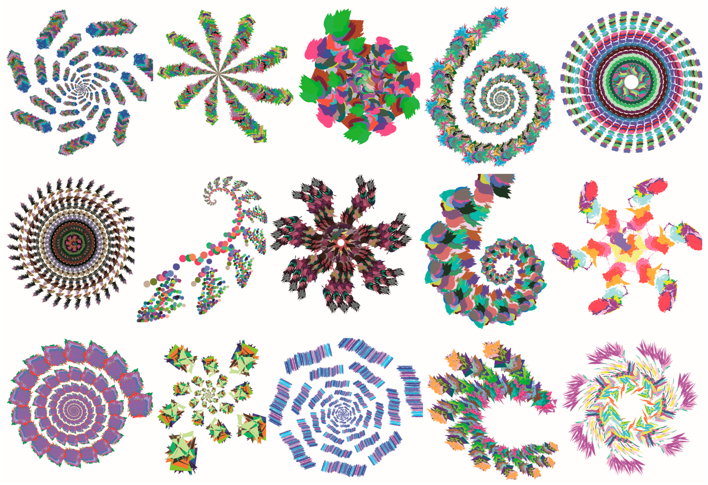
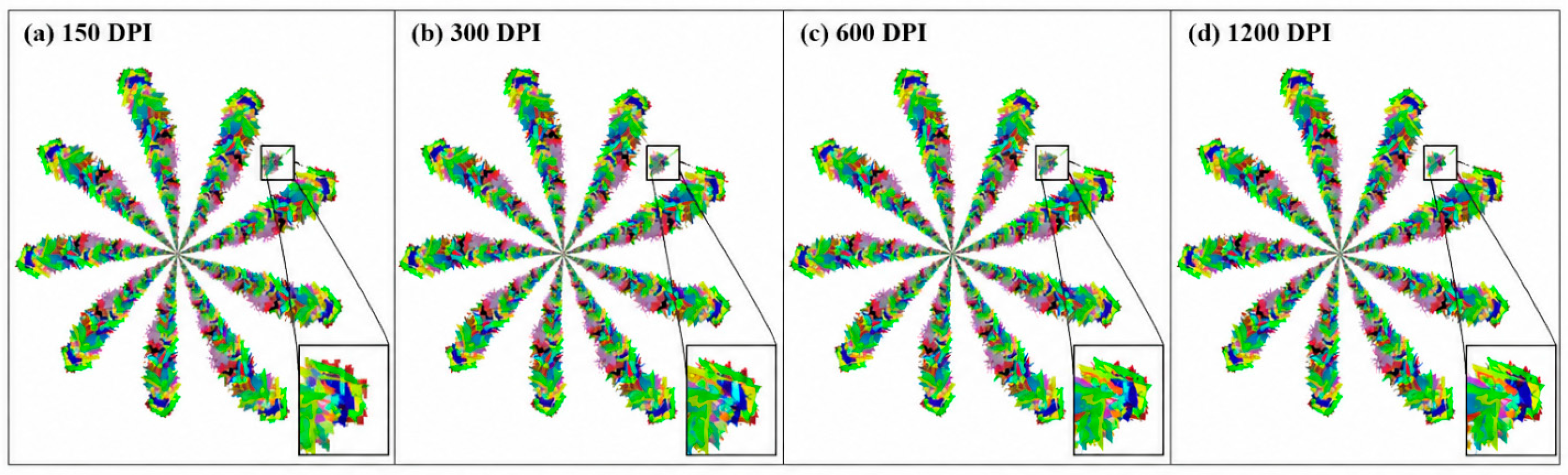
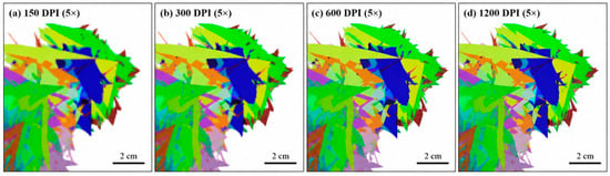
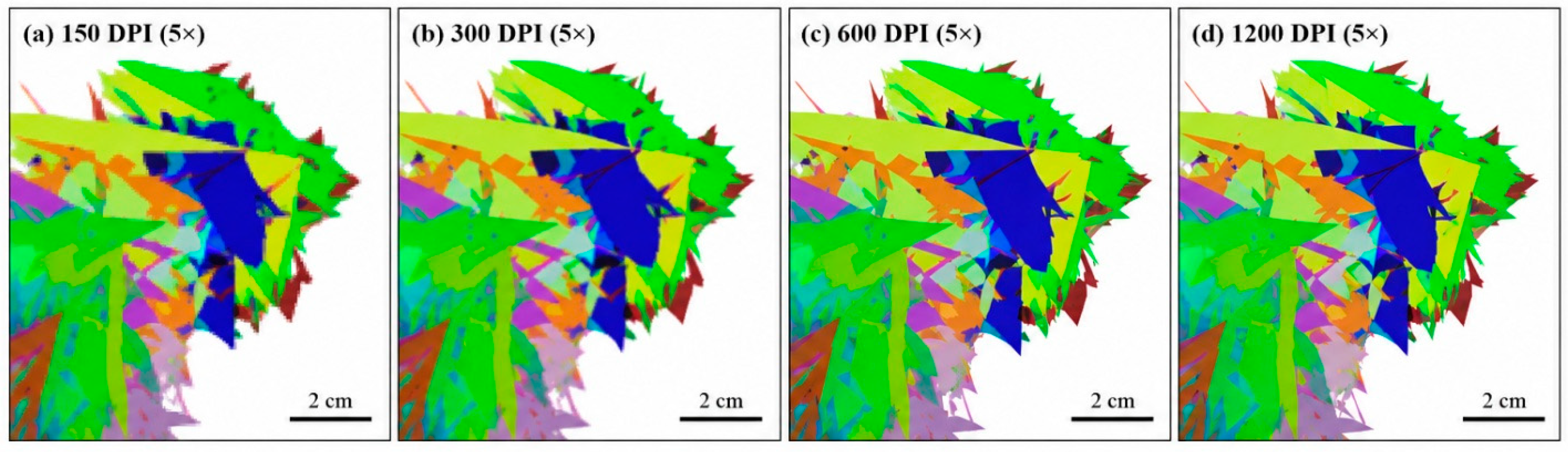
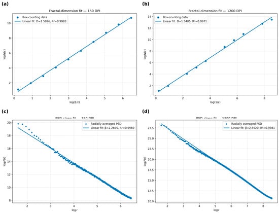
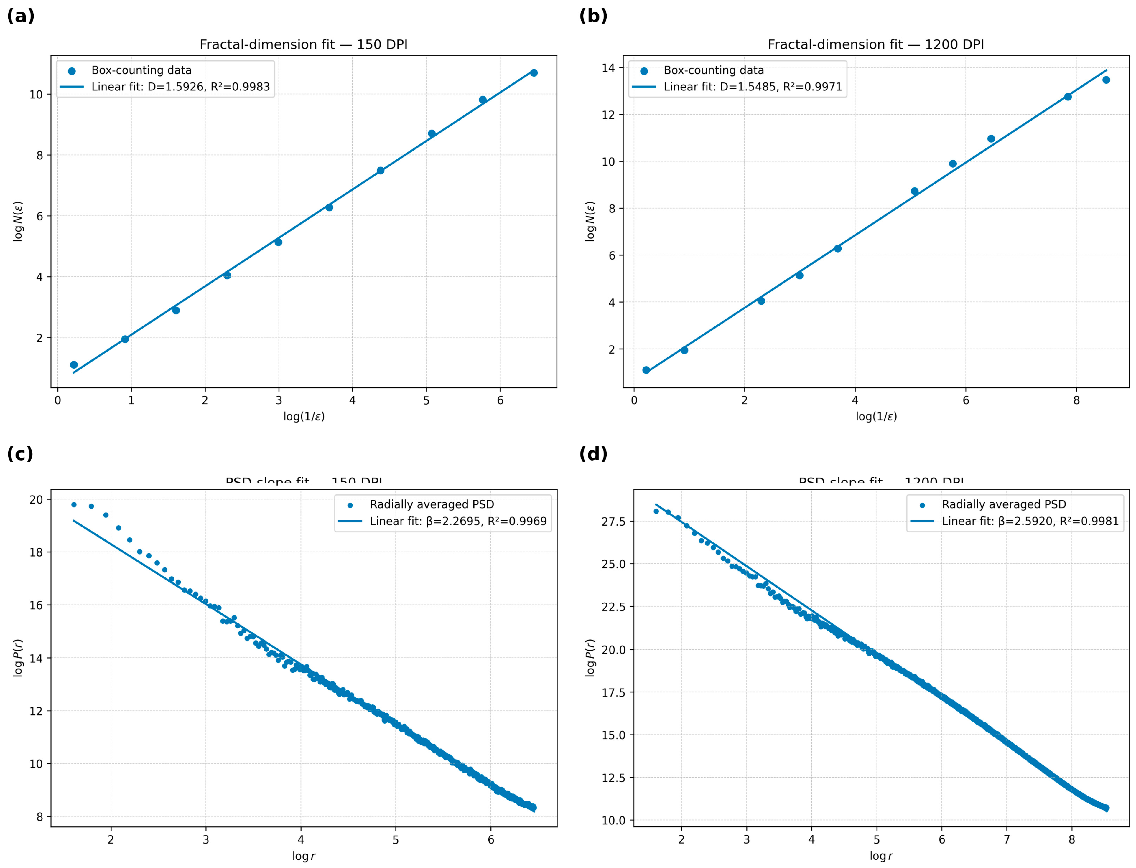
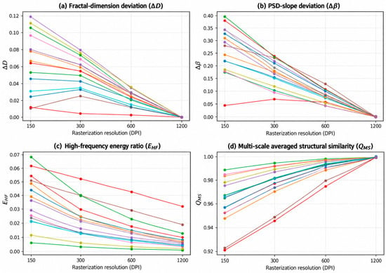
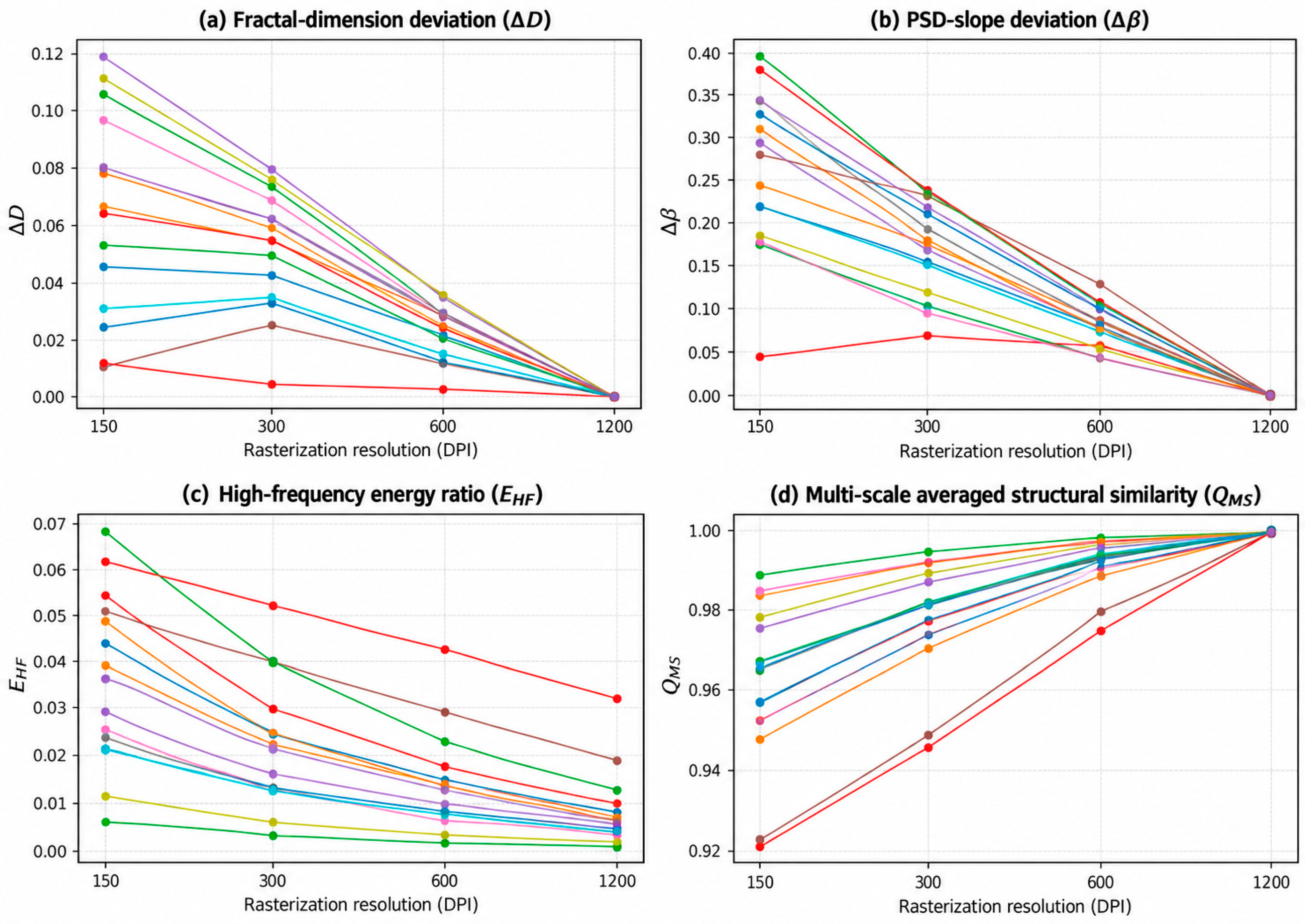
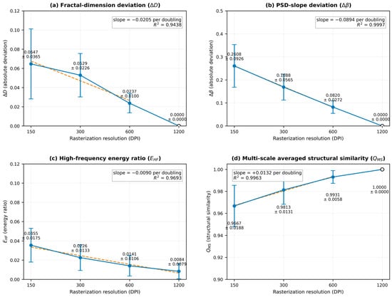
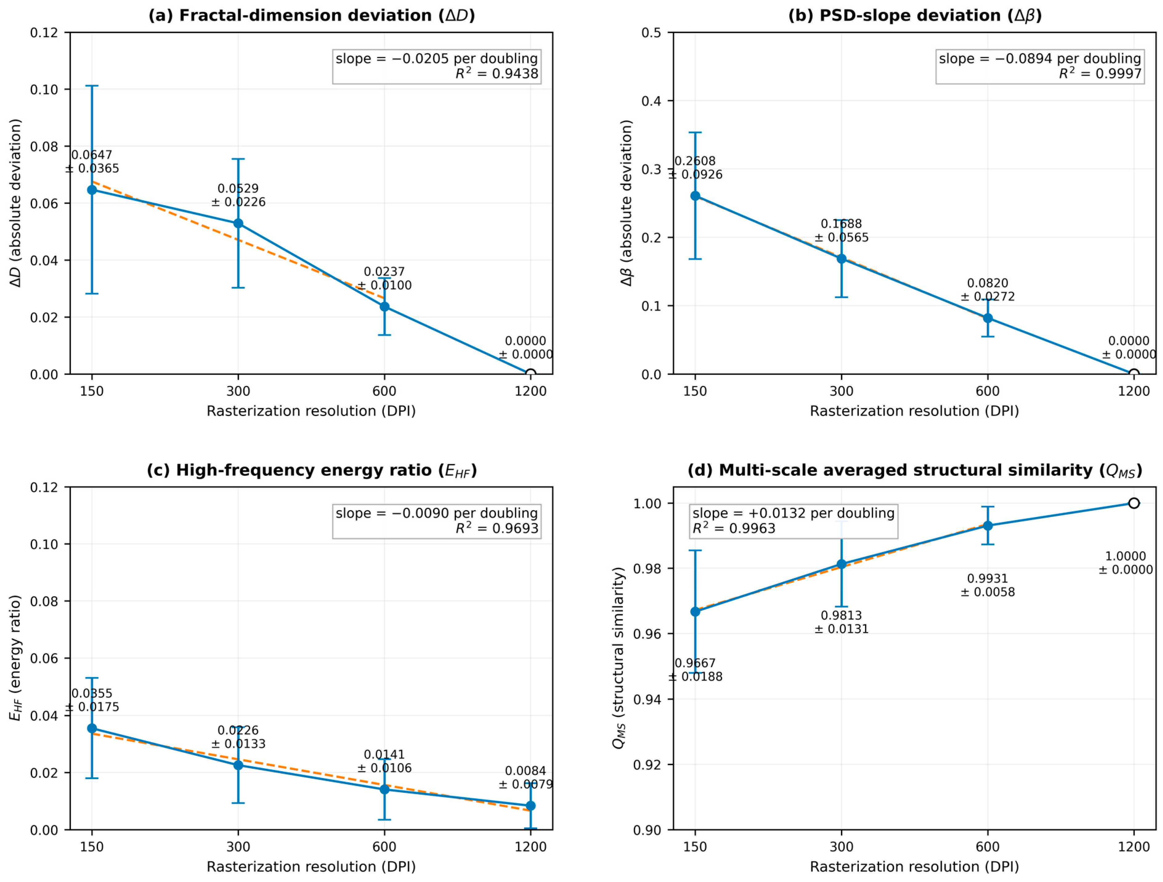

Disclaimer/Publisher’s Note: The statements, opinions and data contained in all publications are solely those of the individual author(s) and contributor(s) and not of MDPI and/or the editor(s). MDPI and/or the editor(s) disclaim responsibility for any injury to people or property resulting from any ideas, methods, instructions or products referred to in the content. |
© 2026 by the authors. Licensee MDPI, Basel, Switzerland. This article is an open access article distributed under the terms and conditions of the Creative Commons Attribution (CC BY) license.