Aerobic and Energy-Recovery Treatment Processes of Sanitary Waste to Reduce End-of-Life Carbon Emissions

Abstract

Greenhouse gas (GHG) emissions from sanitary waste (SW) are not usually quantified in institutional inventories, which limits the ability to assess its management and associated carbon footprint. This study establishes emission factors (EF) for SW generated in a higher education institution (HEI), focusing on toilet paper. In 2022, 19 sanitary waste sources were monitored, obtaining a per capita generation of 3.02 g person⁻¹ day⁻¹ and an annual total of 356.87 kg of SW. Samples were characterized through proximate and elemental analyses, applying stoichiometric calculations for two disposal-site degradation pathways: Aerobic: 841.95 kg (total climate indicator) t⁻¹ SW, and Anaerobic: 7041.97 kg (total climate indicator) t⁻¹. The arithmetic mean of the aerobic and anaerobic EFs was 3941.96 kg (total climate indicator) t⁻¹ SW. Based on an estimated annual mass of 1.12 t yr⁻¹, emissions ranged from 0.35 to 6.71 t yr⁻¹ (total climate indicator: CO₂ + CH₄-derived CO₂e) depending on the scenario. Emissions could be reduced by over 90% when aerobic degradation or controlled methane capture predominates. The results suggest that separating SW at its point of generation and ensuring that it undergoes aerobic or energy-recovery treatment processes can limit its contribution to institutional GHG inventories. Having material-specific EF enables quantitative comparison among management strategies and guides continuous-improvement decisions.

1. Introduction

Inadequate disposal of solid waste generates multiple environmental and public health impacts, including odor emissions, leachate formation, pathogen proliferation, and greenhouse gas (GHG) release. GHG emissions are a major international concern due to their environmental, economic, and social implications. Waste generation is influenced by socioeconomic factors, consumption habits, collection services, and sociocultural conditions. While the waste sector contributes a relatively small share of global GHG emissions, interest in quantifying its contribution and identifying effective mitigation strategies has increased substantially.

Globally, municipal solid waste (MSW) generation is estimated at 5.5 million t day⁻¹, with per capita values ranging from 0.11 to 4.54 kg person⁻¹ day⁻¹ [1]. In Mexico, MSW generation reaches approximately 120,128 t d⁻¹, with a national per capita average of 0.944 kg person⁻¹ day⁻¹, and about 72% of this waste is disposed of in sanitary landfills [2]. In Tabasco [2], MSW generation totals 2471 t d⁻¹, corresponding to 0.867 kg person⁻¹ day⁻¹, yet only 2.31% is properly managed relative to national and international standards [3]. Regarding GHG emissions, the waste sector contributes 160,471 Gg CO₂-equivalent (CO₂e) globally (5% of total emissions) [1], 29,029 Gg CO₂e in Mexico (4.41%) [2], and 1093 Gg CO₂e in Tabasco (3.13% of state emissions) [3].

MSW typically consists of inorganic materials with economic value (plastics, metals, paper, electronics) and organic fractions that are less studied yet environmentally relevant, such as sanitary waste (SW). Li et al. [4] report the annual per capita consumption of toilet paper (TP) and its variation according to economic and demographic factors. Reported annual TP consumption in some countries includes 22.68 kg in the United States, 12.57 kg in Eastern Europe, 10.83 kg in Japan, 4.20 kg in Latin America, 2.90 kg in China, and 0.40 kg in Africa. These values suggest an average TP generation of approximately 0.017 kg person⁻¹ day⁻¹, with a median of 0.012 kg person⁻¹ day⁻¹.

Sanitary waste (SW) generated in restroom facilities poses health risks due to the presence of persistent enteric pathogens, requiring appropriate treatment technologies. Pathogens such as Bacteroides, Faecalibacterium and Prevotella [5], which are associated with gastrointestinal diseases including salmonellosis, hepatitis, ascariasis, giardiasis, rotavirus, exhibit high environmental persistence [6]. Therefore, appropriate treatment methods, ranging from sanitary landfill disposal to incineration and wastewater treatment are required. In wastewater systems, cellulose from TP can be hydrolyzed and metabolized, contributing 25.5 ± 0.6% CH₄ from 2.02 g COD L⁻¹ day⁻¹ [7]. Although landfilling remains the primary disposal method, TP decomposes slowly because of its cellulose content and low nitrogen and phosphorus levels [8]. Bridle et al. [9] reported that unbleached paper degrades 2.8 times faster than bleached paper after six months, indicating that environmental conditions and the deposition of organic matter (feces and urine) strongly influence the degradation process.

An understudied aspect of SW is its contribution to GHG emissions, which requires standardized estimation methods to establish management targets and performance indicators. Clabeaux et al. [10] indicate that assessing GHG emission sources can guide the formulation of mitigation objectives, strategies, and policies to reduce GHG emissions in public and private sectors. Emission factors (EFs) are a methodological tool that enable practical and cost-effective quantification of emissions, expressed in mass units (kg or t) as CO₂e per unit of material, product, or service [11].

Higher education institutions (HEIs) contribute to sustainability agendas aligned with the SDGs [12] and increasingly quantify greenhouse gas (GHG) emissions using carbon footprint (CF) or inventory-based approaches. However, published waste-related results remain difficult to compare across campuses due to heterogeneous reference years, activity indicators (e.g., population), and boundary/scope definitions (e.g., Scopes 1–2 vs. Scopes 1–3). To improve transparency, Table 1 summarizes selected HEI studies and reports the contextual descriptors required for interpretation (year, campus size/population indicator, waste-related scope, and boundary notes).

Table 1. Reported GHG metrics for university waste and boundary context (literature benchmark).

Institution (Country)	Year(s)	Campus Size/Population	Waste-Related Scope	Key Reported Metric & Boundary Note
USTP–Oroquieta (Philippines) [13]	2022	1252 (avg. students + employees)	Campus inventory (waste not disaggregated)	Total 38.8910 tCO2e (Scopes 1–2); 0.0311 tCO2e cap−1; Scope 2 dominates (electricity)
Universitas Pertamina (Indonesia) [14]	2017–2018	ND	Solid waste included (modeled)	Solid waste 14.08 tCO2e yr−1 within total CF (~1352 tCO2e yr−1); inventory-based; WARM for waste; landfill disposal modeled
Technological University of Pereira (Colombia) [15]	2017–2018	22,501 people (reported)	Waste included in Scope 3	Total CF 8969 tCO2e yr−1; 0.4 tCO2e person−1 yr−1 (2017); GHG Protocol Scopes 1–3
Imperial College London, Chem. Eng. Dept. (UK) [16]	FY2018/19–FY2019/20	187 staff (students ND)	Dept. CF (waste not isolated)	7620–8330 tCO2e; department boundary; Scopes 1–3 (Scope 3 dominates)
University of Cape Town (South Africa) [17]	2007	ND	Solid waste + paper products + wastewater	Total CF 84,925.5 tCO2e yr−1; solid waste 595.1 and paper 278.9 tCO2e yr−1; IPCC-based inventory
University of Haripur (Pakistan) [18]	ND	3400 students; 410 staff	Campus CF (waste minor)	Total CF ~579 tCO2e; operational boundary; waste ~1% of total; SimaPro/IPCC
Universiti Teknologi Malaysia (Malaysia) [19]	ND	ND	Composting (food + green waste)	EF 0.111 tCO2e t−1 feedstock; boundary includes transport + shredding/diesel + fugitive CH4/N2O
Yildiz Technical University (Turkey) [20]	2019–2020	34,138 students; 2386 staff	Domestic waste within campus CF	Domestic waste CO2e reported (within total CF); campus boundary; exclusions noted (e.g., Technopark)
Universidad Juárez Autónoma de Tabasco—DACBiol (Mexico) [21]	2017	2100 people	Campus MSW management (recovery + disposal)	MSW generation 31.05 t yr−1; 146.5 kg d−1; 0.07 kg d−1 cap−1; stoichiometric EF for OFMSW + bibliographic EFs

Note: ND = not disclosed/not reported; reported metrics vary by boundary definition, reference year, and normalization, limiting direct comparability.

Overall, the literature indicates that waste-related results in HEIs are reported under heterogeneous boundaries and normalization choices, limiting cross-campus comparisons. Moreover, sanitary waste (SW) is rarely treated as a distinct waste stream, with SW-specific emission factors derived from transparent assumptions, which constrains benchmarking and mitigation planning in HEIs.

Collectively, Table 1 highlights that differences in waste definitions, functional metrics (total vs. fraction-specific vs. per capita), and declared boundaries limit direct cross-campus comparison. Importantly, although paper products may implicitly include sanitary components (e.g., toilet paper), CO₂e information specifically focused on sanitary waste (SW) remains scarce and is often embedded within broader categories rather than treated as a distinct waste stream. Therefore, SW-specific emission factors are needed to support consistent estimation and benchmarking of GHG impacts in HEIs. Accordingly, the objective of this study is to estimate SW-specific emission factors using stoichiometric calculations and to quantify scenario-based annual results (t yr⁻¹) using a total climate indicator (CO₂ + CH₄-derived CO₂e, GWP₁₀₀) for SW generated and managed at DACBiol-UJAT during 2022. This approach enables a transparent comparison of management scenarios and supports the integration of SW into institutional GHG inventories.

2. Materials and Methods

2.1. Waste Management at CATRE

The study area corresponded to the university community of DACBiol-UJAT (Tabasco, Mexico). The campus operates a Waste Collection and Treatment Center (CATRE), which receives solid waste generated from academic and administrative activities. Waste originates from classrooms, administrative and faculty offices, laboratories (excluding hazardous laboratories), the library, auditoriums, computer centers, cafeterias, points of sale, and restroom facilities.

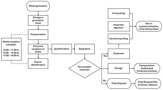
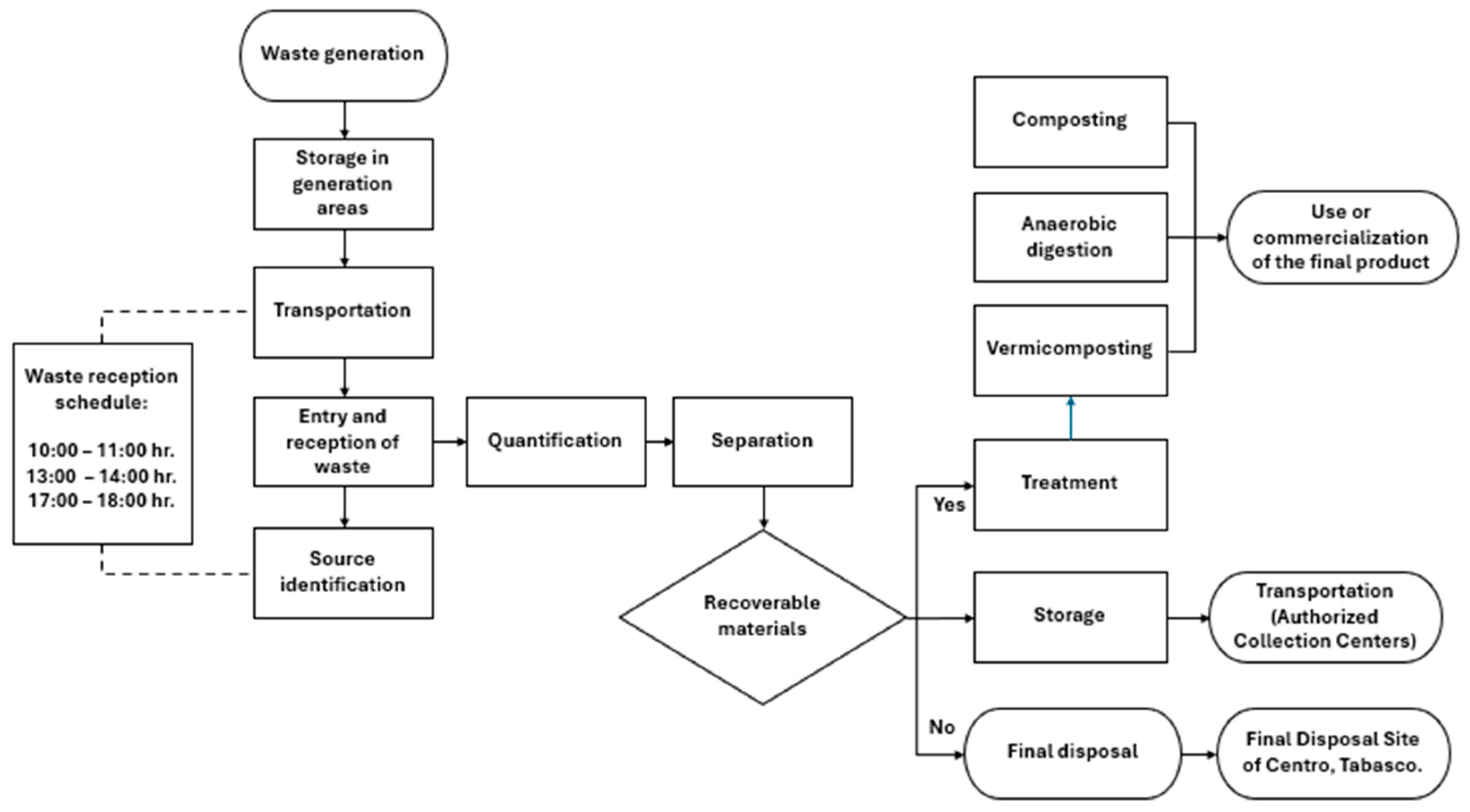
Waste management begins at designated collection points, where custodial staff gather the material. The waste is then transported to the CATRE according to pre-established collection schedules. Upon arrival, the waste is identified, quantified, recorded, separated, and either treated on-site or sent for final disposal through the institutional collection service, as shown in Figure 1.

Figure 1. Waste management at CATRE of DACBiol (source: own elaboration).

Sanitary waste (SW) generation was recorded during two academic semesters in 2022: Semester 2022-1 (February–July) and Semester 2022-2 (August–January 2023). Quantification was performed using a digital scale (model HW-200KVWP; capacity: 200 kg; resolution: 50 g; A&D Weighing, Ann Arbor, MI, USA). Records were initially documented in a physical logbook and subsequently transferred to digital format for statistical analysis.

The average daily generation (G_d) was calculated from the total annual generation (G_SW), considering the effective working days in the year (D_ef), according to Equation (1):

$$G_d= {\displaystyle \frac{G_{SW}}{D_{ef}}}$$

(1)

where G_SW is the total SW generated during 2022 (kg), D_ef is the number of effective working days, and G_d is the average daily generation (kg day⁻¹). Per capita generation (G_pc) was calculated by dividing the daily generation (G_d) by the total campus population (P_t) during 2022, as shown in Equation (2):

$$G_{pc}= {\displaystyle \frac{G_d}{P_t}}$$

(2)

where G_pc is expressed as grams per person per day.

2.2. System Boundary

This study applies a scenario-based, process-focused boundary limited to emissions generated during the end-of-life management of sanitary waste (SW) in a university context. The assessment includes the stoichiometric formation of biogenic CO₂ and CH₄ from SW under aerobic and anaerobic pathways and, where applicable (Scenario B), CH₄ capture and combustion. Results are reported using a total climate indicator defined as CO₂ (factor 1 within the climate indicator) + CH₄-derived CO₂e (GWP100), following the accounting convention described below.

The functional unit (FU) is 1 tonne of sanitary waste (1 t SW), used to express emission factors in kg (total climate indicator) t⁻¹ SW and to scale annual scenario totals using the annual reference mass (ARM).

This work is not a life cycle assessment; it is a scenario-based end-of-life GHG emissions assessment focused on degradation and methane management at the disposal stage. It excludes upstream production burdens (e.g., sanitary paper manufacturing) and operational processes such as collection, transport, and landfill infrastructure/operation. Table 2 presents the included and excluded processes.

Table 2. System boundary definition for the scenario-based assessment (included and excluded processes).

Category	Included	Excluded
SW quantification	Recorded SW (GSW) and annual reference mass (ARM) normalization	-
End-of-life degradation (core)	Stoichiometric formation of biogenic CO2 and CH4 (aerobic vs. anaerobic)	-
CH4 management & climate metric	Scenario B: CH4 capture and combustion; uncaptured CH4 emitted. Total climate indicator = CO2 (factor 1) + CH4-derived CO2e (GWP100)	CH4 oxidation in cover soils (base case)
Upstream & operational processes	-	Paper manufacturing; collection/transport; landfill operations/infrastructure energy

Note: Excluded processes were not quantified due to lack of site-specific activity data and because the study focuses on end-of-life degradation pathways and CH₄ control.

2.3. Stoichiometric Calculations of Sanitary Waste Emission Factors

Representative SW samples were collected following the quartering method established in NMX-AA-015-1985 for solid waste. Subsamples of 10 g were subjected to proximate analysis according to ASTM D2974 to determine moisture (105 °C, 24 h), volatile solids (550 °C, 2 h), and ash content (800 °C, 1 h) [22,23]. Fixed carbon content was subsequently calculated by difference.

Elemental composition (C, H, N, and S) was determined using oven-dried samples analyzed with a Perkin Elmer^® PE2400 CHNS/O elemental analyzer (PerkinElmer, Inc., Waltham, MA, USA). Oxygen content was calculated by difference, subtracting the sum of C, H, N, S, and ash from 100% on a dry-weight basis, as shown in Equation (3).

$$O=100-\left[\left(C+H+N+S\right)+Ash\right]$$

(3)

The elemental composition data was used to derive empirical chemical formulas of the form C_aH_bO_cN_dS_e. Elemental percentages were converted to molar ratios, and formulas were normalized to one mole of nitrogen and one mole of sulfur, following the method of Tchobanoglous et al. [24], where these elements are treated as limiting nutrients during biological degradation.

Stoichiometric calculations were performed to estimate the theoretical maximum gas production during aerobic and anaerobic biological degradation [24]. Aerobic conversion was estimated using Equation (4), and anaerobic conversion applying Equation (5):

$$C_a{H}_b{O}_c{N}_d+\left({\displaystyle \frac{4_a+b-2_c-3_d}{4}}\right)O_2 \to a{CO}_2+\left({\displaystyle \frac{b-3d}{2}}\right)H_{2}O+dN{H}_3$$

(4)

$$C_a{H}_b{O}_c{N}_d+\left(a-{\displaystyle \frac{b}{4}}-{\displaystyle \frac{c}{2}}+{\displaystyle \frac{3d}{4}}+{\displaystyle \frac{e}{2}}\right)H_{2}O\to \left({\displaystyle \frac{a}{2}}+{\displaystyle \frac{b}{8}}-{\displaystyle \frac{c}{4}}-{\displaystyle \frac{3d}{8}}-{\displaystyle \frac{e}{4}}\right){CH}_4+\left({\displaystyle \frac{a}{2}}+{\displaystyle \frac{b}{8}}-{\displaystyle \frac{c}{4}}-{\displaystyle \frac{3d}{8}}-{\displaystyle \frac{e}{4}}\right){CO}_2+{dNH}_3+H_{2}S$$

(5)

A step-by-step derivation of the stoichiometric coefficients and scaling to the functional unit (Table 3C) is provided in Supplementary Information S2.

Table 3. Proximate and Ultimate Composition of Sanitary Waste.

A	Analytics (%)				Elementals (%)
	Moisture	Volatile Matter	Fixed Carbon	Ash	C	H	O	N	S
	9.78 ± 7.17	91.28 ± 1.42	2.39 ± 1.10	6.31 ± 1.53	42.08 ± 0.03	6.26 ± 0.01	49.91	0.96 ± 0.08	0.25 ± 0.02
B	Process			Chemical Formulas			Condition
	Aerobic			$C_{50.98}{H}_{17.51}{O}_{9.86}{N}_1$			Without sulfur; with water
	Anaerobic			$C_{449.49}{H}_{154.38}{O}_{86.92}{N}_{8.82}{S}_1$			With sulfur; with water
C	Theoretical gas production from sanitary waste (biogenic CO2 and CH4) and CH4-derived CO2e (GWP100)
	Process	CO2 (t t−1 SW)	CH4 (t t−1 SW)		CH4-derived CO2e (t t−1 SW)		Total climate indicator (t t−1 SW)
	Aerobic	0.8419	-		-		0.8419
	Anaerobic	0.6595	0.2279		6.3823		7.0419

Note: CO₂ and CH₄ originate from biogenic carbon in sanitary paper. CH₄ is converted to CO₂e using GWP₁₀₀ (CH₄ = 28). The reported “Total climate indicator” is computed as CO₂ (treated with factor 1) + CH₄-derived CO₂e for scenario comparison. For inventory-style reporting, biogenic CO₂ can be disclosed separately.

Methane (CH₄) and carbon dioxide (CO₂) were converted to CO₂e units using their respective global warming potential (GWP₁₀₀) values reported by the IPCC (GWP₁₀₀ = 28 for CH₄), as expressed in Equation (6):

$${CO}_{2e}=GHG mass\times GWP$$

(6)

The SW considered in this study is primarily of biogenic origin (sanitary paper). Accordingly, CO₂ and CH₄ generated from SW are biogenic. For inventory-style reporting, biogenic CO₂ is disclosed separately following IPCC convention, while CH₄ is expressed as CO₂e using GWP₁₀₀ (CH₄ = 28). For scenario comparability, we additionally report a “total climate indicator” computed as CO₂ (treated with factor 1) + CH₄-derived CO₂e. This convention avoids ambiguity between physical mass flows (CO₂, CH₄) and climate-equivalent metrics (CO₂e).

Emission factors (EFs) for aerobic and anaerobic degradation were calculated on a mass basis kg (total climate indicator) t⁻¹ SW from the stoichiometrically estimated gas production, as defined in Equation (7a,b). In Equation (7a,b), m_SW denotes the sanitary waste mass basis (1 t SW) used to express emission factors in kg (total climate indicator) t⁻¹ SW.

$$FE (Aerobic)={\displaystyle \frac{{CO}_2}{m_{SW}}}$$

(7a)

$$FE (Anaerobic)={\displaystyle \frac{{CH}_4}{m_{SW}}}$$

(7b)

Total GHG emissions were then estimated by multiplying the annual reference mass (ARM) by the respective aerobic or anaerobic emission factor (EF), as shown in Equation (8), yielding values expressed in t yr⁻¹ (total climate indicator: CO₂ + CH₄-derived CO₂e). The recorded annual mass (GSW) is reported for transparency, whereas ARM is used for scenario-based emission estimates to avoid underestimation due to days without recorded entries.

$${kg CO}_{2e}=ARM\times EF$$

(8)

2.4. Emissions Balance

2.4.1. Reference Mass and Annual Extrapolation

The reference mass (RM) was projected from the SW recorded during the effective sampling days in 2022 (D_FM). To obtain an annual estimate, an extrapolation factor (F_EX) was calculated based on the ratio between total operational days (D_EA) and effective sampling days (D_FM), as expressed in Equation (9). The annual reference mass (ARM) was then obtained by multiplying the F_EX by the annual SW generation (G_SW), as expressed in Equation (10):

$$F_{EX}={\displaystyle \frac{D_{EA}}{D_{FM}}}$$

(9)

$$ARM=F_{EX}\times G_{SW}$$

(10)

The reference mass was subsequently used to estimate emissions based on the stoichiometrically calculated EF for each degradation pathway.

2.4.2. The Three Emission Scenarios Evaluated

1.

Scenario A—Anaerobic degradation without CH₄ capture

This scenario assumes complete anaerobic degradation with no methane capture. Total emissions (S_A) were obtained by multiplying the anaerobic EF by the annual reference mass (ARM), as expressed in Equation (11):

$$S_A={FE}_{anaerobic}\times ARM$$

(11)

2.

Scenario B—Anaerobic degradation with 75% CH₄ capture and combustion

In this scenario, 75% of methane is assumed to be captured and oxidized to CO₂, following IPCC standard practice for landfills with venting/flare systems [25,26]. The remaining 25% of CH₄ retains its original GWP₁₀₀ (28). The resulting EF was calculated using Equation (12), and scenario B emissions (S_B) were obtained using Equation (13).

$${FE}_{resulting}={FE}_{aerobic}+\left[0.25\times \left({FE}_{anaerobic}-{FE}_{aerobic}\right)\right]$$

(12)

$$S_B={FE}_{resulting}\times ARM$$

(13)

3.

Scenario C—Predominantly aerobic degradation (complete oxidation)

This scenario assumes that SW undergoes primarily aerobic degradation. Total emissions ($S_C$) were calculated by multiplying the aerobic EF by the annual reference mass (ARM), as expressed in Equation (14):

$$S_C= {FE}_{aerobic}\times ARM$$

(14)

A compact one-at-a-time sensitivity analysis (capture efficiency range, ±20% yield/degradability envelope, and a GWP time-horizon note) is reported in Supplementary Information S1 (Table S1) to document the robustness of the scenario comparisons.

3. Results

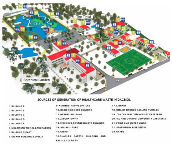
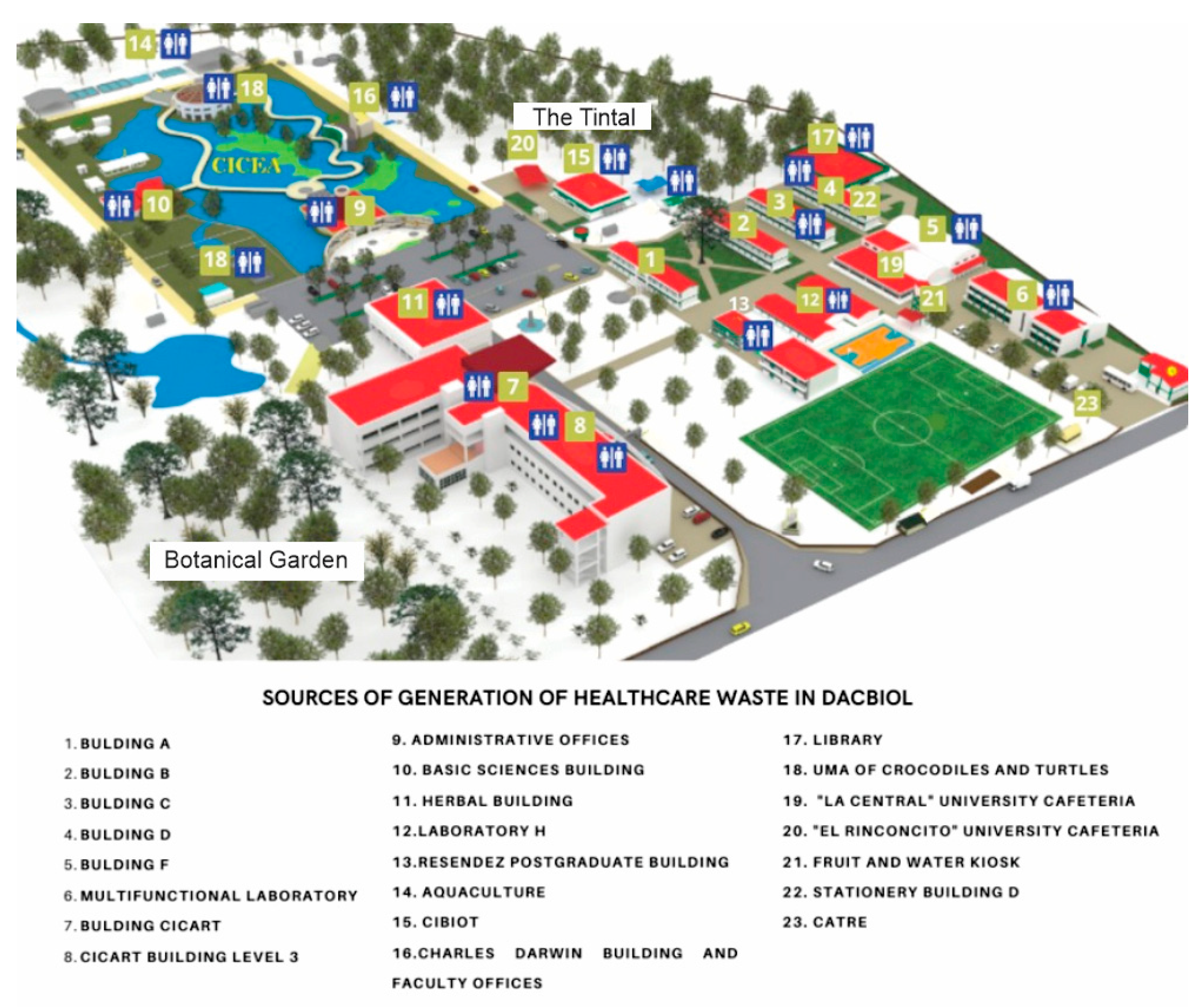
Figure 2 shows the distribution of SW generation sources within DACBiol-UJAT, highlighting the 19 facilities equipped with restroom services that contributed to the measurements conducted in this study.

Figure 2. Generation sources with sanitary facilities at DACBiol-UJAT (source: DACBiol-UJAT).

A total of 23 waste generation sources were identified across the campus; however, only 19 of them included sanitary facilities and were therefore considered in the SW analysis.

3.1. SW Generation

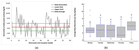
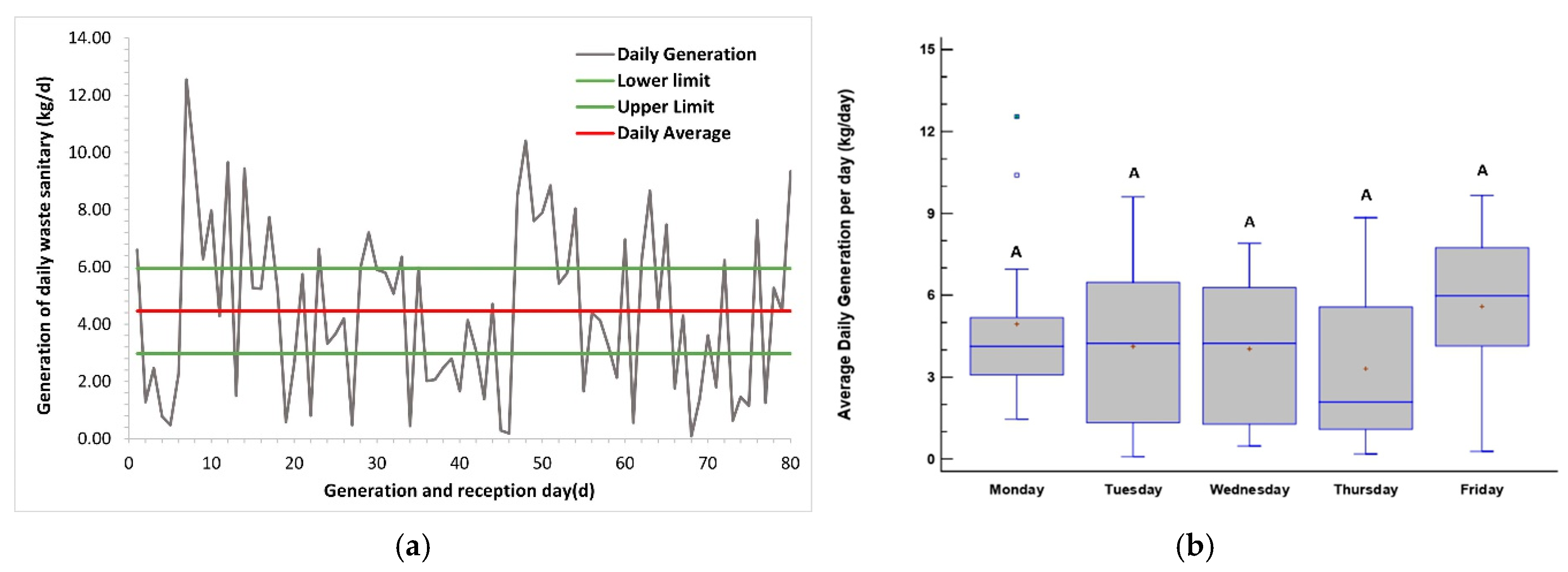
In 2022, the total MSW generation at DACBiol-UJAT was 17.96 t. While the academic calendar included 251 operational days, only 204 were considered effective working days, and SW entries to CATRE were recorded on 80 of those days (Figure 3a).

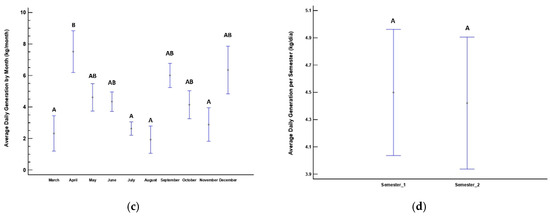
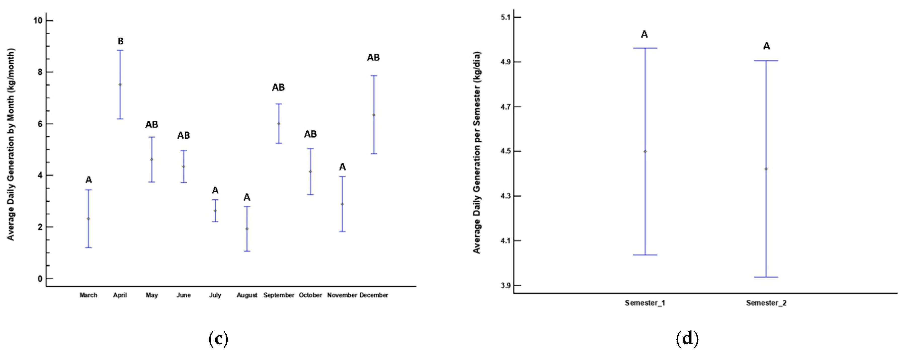
Figure 3. SW generation at DACBiol during 2022; (a) daily SW generation and average; (b) weekly average SW generation; (c) monthly average SW generation; (d) SW generation by semester period. Letters above the means (A, B, AB) indicate the homogeneous groups obtained from the one-way ANOVA followed by Bonferroni post hoc comparisons. Means sharing at least one letter are not significantly different (p ≥ 0.05), whereas means with different letters are significantly different (p < 0.05). In boxplots, the “+” symbol denotes the mean and dots indicate outliers (the horizontal line within each box represents the median).

Annual SW generation was 356.87 kg yr⁻¹, equivalent to 7.5% of the total MSW generation. The average monthly generation was 35.69 ± 23.20 kg (n = 10), and the daily generation was 4.46 ± 2.97 kg (n = 80). Considering a campus population of 1477 individuals, the per capita generation was 3.02 g person⁻¹ day⁻¹.

The value of 356.87 kg yr⁻¹ corresponds to the recorded SW mass on days with registered entries, whereas the annual reference mass (ARM) represents the extrapolated annual mass used for scenario-based emission estimates. The ARM, extrapolated from effective sampling days, was 1.12 t yr⁻¹ SW, obtained using the extrapolation factor described in Equation (9). This distinction helps avoid underestimation due to days without recorded entries.

$$Extrapolation Factor={\displaystyle \frac{251 actual effective days}{80 sampling days}}=3.14$$

$$Annual Reference Mass \left(SW\right)=(3.14\times {356.87 \mathrm{kg} \mathrm{yr}}^{-1})=1.12 \mathrm{t} {\mathrm{yr}}^{-1}$$

Comparison with other cases may be limited due to differences in institutional activities, student populations, and the number of effective operational days. Aguilar-Virgen et al. [27] reported a generation of 18.20 kg week⁻¹ in a building with 80 resident students (0.0325 kg person⁻¹ day⁻¹), while Smyth et al. [28] reported 2.10 t week⁻¹ of MSW at a Canadian university, with paper towels accounting for 13% of the total. These values underscore the variability in SW generation patterns across HEIs.

3.2. Statistical Analysis of Temporality

The results were analyzed using parametric and non-parametric statistical tests. Figure 3b–d show the one-way ANOVA results of SW generation behavior over different time periods.

Daily SW generation showed no significant differences between weekdays (Kruskal–Wallis test, p = 0.149). In contrast, one-way ANOVA revealed statistically significant differences across months (p = 0.006), particularly in April, which showed the largest deviation.

Post hoc Bonferroni analysis grouped the months into three statistically distinct clusters: Group A (March, July, August, November), Group B (April), and Group AB (May, June, September, October, and December). April formed an independent cluster due to its markedly higher SW values.

The semester-based analysis showed no statistically significant differences (p = 0.908). Overall, temporality did not exhibit a statistically significant effect on SW generation, despite variations observed on specific days and months (Figure 3).

3.3. Limitations in Quantification

A recurring limitation in the quantification process was the frequent mixing of sanitary waste (SW) with the remaining municipal solid waste (MSW). For biosafety reasons, CATRE personnel were restricted from handling MSW bags that contained visible SW, which reduced the amount of usable data and introduced uncertainty in daily records.

To mitigate this issue, waste bags arriving from each sanitary facility were required to include an inner secondary bag designated exclusively for SW, ensuring proper segregation and minimizing data loss during subsequent measurements.

3.4. Emission FACTORS (EF) Calculated from SW

Table 3A summarizes the proximate and elemental composition of SW, whereas Table 3B shows the empirical chemical formulas derived from these data. These formulas were used to estimate the theoretical stoichiometric production of CO₂ and CH₄ under aerobic and anaerobic conditions (Table 3C).

Elemental composition values (C, H, O, N, S) were generally consistent with those reported for toilet paper and similar cellulose-based materials [7,8]. However, nitrogen and sulfur contents were lower than values reported for fecal matter, particularly nitrogen (5.4% in Kim et al. [8]), which is expected since the samples consisted primarily of toilet paper with limited fecal contamination. This composition directly influenced the stoichiometric gas yields and, consequently, the emission factors reported in Table 4.

Table 4. Calculated EF and Ranges for Sanitary Waste.

Process	EF Expressed as Kg (Total Climate Indicator) t−1 SW
Aerobic	841.95
Anaerobic	7041.97
Arithmetic mean	3941.96

Table 3C summarizes the theoretical yields of biogenic CO₂ and CH₄ per functional unit (1 t SW) under aerobic and anaerobic pathways. In Route A, CO₂ is included with a factor of 1 within the total climate indicator, whereas CH₄ is converted to CH₄-derived CO₂e using GWP₁₀₀ (CH₄ = 28). Accordingly, the anaerobic pathway yields a total climate indicator of 7.0419 t t⁻¹ SW, dominated by CH₄-derived CO₂e, while the aerobic pathway results in 0.8419 t t⁻¹ SW. For comparison of pathway magnitudes, the sum of these pathway totals is 7.883 t t⁻¹ SW; however, this combined value should not be interpreted as a single-process result.

Table 4 presents the stoichiometrically derived emission factors (EF), expressed as kilograms of total climate indicator per metric ton of sanitary waste (kg (total climate indicator) t⁻¹ SW), for both aerobic and anaerobic degradation pathways.

Aerobic degradation produced an EF of 841.95 kg (total climate indicator) t⁻¹ SW, whereas anaerobic degradation yielded a substantially higher EF of 7041.97 kg (total climate indicator) t⁻¹ SW due to methane production. This difference illustrates the strong influence of the selected degradation pathway on the climate impact of SW.

Using the arithmetic mean of the aerobic and anaerobic EFs, 3941.96 kg (total climate indicator) t⁻¹ SW, annual emissions for the 1.12 t SW yr⁻¹ were estimated at 4.41 t _yr⁻¹ (total climate indicator: CO₂ + CH₄-derived CO₂e). As expected, aerobic degradation produced the lowest emissions, whereas anaerobic conditions resulted in substantially higher values due to methane formation.

The annual emission estimate of 4.41 t yr⁻¹ (total climate indicator: CO₂ + CH₄-derived CO₂e) is higher than values reported by other HEIs. Letete et al. [17] reported 1.2 t CO₂e yr⁻¹ for paper waste at the University of Cape Town using life cycle assessment methods, while Aguilar-Virgen et al. [27] recorded 0.297 t CO₂e yr⁻¹ in a university residence in Mexico, and Ullah et al. [18] reported 0.75 t CO₂e yr⁻¹ for paper waste in Pakistan. These differences arise from variations in methodological approaches, waste composition, and the use of stoichiometric methane potentials in the present study, which tend to produce conservative (higher) emission estimates compared to field-based measurements.

3.5. Emission Scenarios

In Mexico, NOM-083-SEMARNAT-2003 mandates biogas collection and flaring systems in landfills receiving more than 100 t day⁻¹ of waste, with the objective of reducing GHG emissions from disposal sites. Within this regulatory context, three hypothetical emission scenarios were developed based on the estimated annual sanitary waste (SW) generation and the methane management approach applied in each case. These scenarios represent contrasting degradation pathways and allow evaluation of relative climate impacts under different CH₄ control strategies. The results of each scenario are described below.

1.

Scenario A—Anaerobic degradation without CH₄ capture

$$S_A=\left(7041.97 \mathrm{kg} {CO}_{2e} {\mathrm{t} }^{-1}SW\right)\times \left(1.12 \mathrm{t} SW{\mathrm{yr}}^{-1}\right)\times \left(0.001\right)=7.89 \mathrm{t} {CO}_{2e}{\mathrm{yr}}^{-1}$$

2.

Scenario B—Anaerobic degradation with 75% CH₄ capture and combustion

$$S_B=\left(738.70 \mathrm{kg} {CO}_{2e}\right)+\left[\left(7041.97-738.70 \mathrm{kg} {CO}_{2e}{\mathrm{t}}^{-1}SW\right)\times 0.25\right]=2314.52 \mathrm{kg} {CO}_{2e}{\mathrm{t}}^{-1}SW$$

$$S_B=\left(2314.52 \mathrm{kg} {CO}_{2e}{\mathrm{t}}^{-1}SW\right)\times \left(1.12 \mathrm{t} SW{\mathrm{yr}}^{-1}\right)\times \left(0.001\right)=2.59 \mathrm{t} {CO}_{2e} {\mathrm{yr}}^{-1}$$

3.

Scenario C—Predominantly aerobic degradation (complete oxidation)

$$S_C=\left(841.95 \mathrm{kg} {CO}_{2e}{\mathrm{t}}^{-1}SW\right)\left(1.12 \mathrm{t} SW {\mathrm{yr}}^{-1}\right)\times \left(0.001\right)=0.942 \mathrm{t} {CO}_{2e} {\mathrm{yr}}^{-1}$$

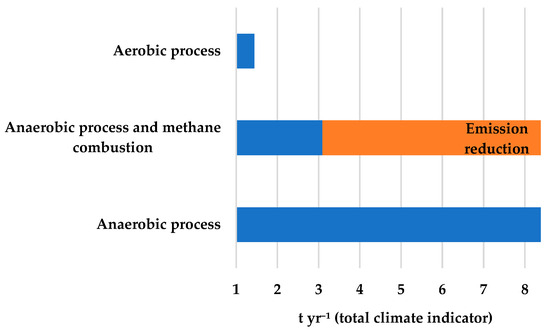
The results of the three scenarios are presented in a comparative bar chart (Excel^® 2021; Microsoft 365; Microsoft Corporation, Redmond, WA, USA).), using a common vertical axis (t yr⁻¹; total climate indicator = CO₂ + CH₄-derived CO₂e) to highlight the relative magnitude (Figure 4). No additional moisture degradation factors were applied, as the EFs already incorporate the actual water content in the stoichiometric calculations.

Figure 4. Scenario-based annual results for sanitary waste management. Values are shown as t yr⁻¹ using the total climate indicator (CO₂ + CH₄-derived CO₂e, GWP100).

When comparing the scenarios, the following observations were made:

• Scenario A represents complete anaerobic degradation without methane capture. Under this condition, emissions reached 7.89 t yr⁻¹ (total climate indicator: CO₂ + CH₄-derived CO₂e), the highest among the modeled scenarios due to uncontrolled methane CH₄ release.

Sensitivity note (Scenario A). Because Scenario A is dominated by methane formation, the total climate indicator is most sensitive to the GWP time horizon used to express CH₄ as CO₂e (a shorter horizon amplifies the methane-driven signal). To reflect uncertainty in waste degradability and the empirical composition/stoichiometric coefficients, a ±20% variation in the stoichiometric gas yields would translate into an approximately proportional change in the Scenario A total, without affecting the qualitative conclusion that uncontrolled anaerobic degradation represents the highest climate penalty.

• Scenario B assumes 75% methane capture and flaring, following IPCC recommendations for controlled landfill operations. This scenario resulted in emissions of 2.59 t yr⁻¹ (total climate indicator: CO₂ + CH₄-derived CO₂e), corresponding to a 67% reduction relative to Scenario A. The remaining 25% of methane, assumed to remain uncaptured, accounts for the residual climate impact.

Sensitivity note (Scenario B). Methane capture performance is the main driver of uncertainty in Scenario B. We tested capture efficiencies of 50%, 75% (base), and 90%, assuming uncaptured CH₄ is emitted directly. Under this range, Scenario B totals remain substantially lower than Scenario A, and the total climate indicator varies approximately linearly with the uncaptured methane fraction (≈4.36 t yr⁻¹ at 50% capture; 2.59 t yr⁻¹ at 75%; ≈1.53 t yr⁻¹ at 90%). A ±20% variation in stoichiometric gas yields produces proportional shifts in the absolute total but does not change the scenario ranking.

• Scenario C, which assumes predominantly aerobic conditions, resulted in emissions of 0.943 t yr⁻¹ (total climate indicator: CO₂ + CH₄-derived CO₂e), representing an 88% reduction compared with Scenario A. Because aerobic degradation does not generate methane, emissions are limited to stoichiometrically released CO₂ during oxidative decomposition.

Sensitivity note (Scenario C). Scenario C is dominated by biogenic CO₂ (factor 1 within the climate indicator) and assumes negligible CH₄ formation; consequently, the total climate indicator is comparatively insensitive to the choice of GWP time horizon because methane plays a minor role. A ±20% variation in stoichiometric yields would shift the absolute CO₂-related total proportionally, but Scenario C remains the lowest-impact pathway among the scenarios considered.

Across the three scenarios, methane was the primary driver of CO₂e component under anaerobic conditions, accounting for approximately 95% of the CH₄-derived CO₂e, due to its high GWP₁₀₀. In contrast, CO₂ (biogenic) mainly contributes to the mass flow of generated gases, whereas CH₄ dominates the climate-equivalent metric. Partial methane capture (Scenario B) considerably mitigates emissions, while aerobic treatment (Scenario C) nearly eliminates methane formation, limiting emissions to CO₂ derived from stoichiometric oxidation. These results are consistent with previous studies reporting the dominant role of methane control in reducing waste-sector emissions [16,17,18,19,20].

4. Discussion

Overall, the scenario results confirm that the end-of-life degradation pathway is the dominant driver of the reported total climate indicator (defined as CO₂ (factor 1 within the climate indicator) + CH₄-derived CO₂e (GWP₁₀₀)), and that mitigation is therefore governed primarily by CH₄ formation and control rather than by the biogenic CO₂ mass flow: under uncontrolled anaerobic conditions (Scenario A), the climate indicator reaches 7.89 t yr⁻¹, whereas partial CH₄ capture and combustion (Scenario B) reduces the indicator to 2.59 t yr⁻¹ (−67%), and predominantly aerobic conditions (Scenario C) reduce it further to 0.943 t yr⁻¹ (−88%).

When contrasted with reported HEI inventories and campus/department carbon footprints, apparent differences in magnitude are expected because published studies vary widely in reference year(s), activity indicators, functional metrics (total vs. fraction-specific vs. per capita), and—critically—declared boundaries/scopes, with waste often aggregated or treated as a minor contributor relative to electricity, mobility, or procurement, while paper products (sometimes including toilet paper) may be reported without isolating sanitary waste as a distinct stream [16,17,18,19,20]. Methodologically, reporting a total climate indicator (rather than a single “Total CO₂e”) improves transparency by making explicit that only the CH₄ component is converted to CO₂e, and it clarifies why CH₄ dominates the climate signal under anaerobic pathways even when CO₂ (biogenic) may represent a large share of emitted gas mass; in this context, the residual impact under Scenario B is controlled by the assumed capture fraction (i.e., the remaining uncaptured CH₄), so the most influential assumptions for robustness are the stoichiometric coefficients derived from the adopted waste composition parameters and the CH₄ capture performance (and any oxidation treatment, if later considered).

Practically, these findings indicate that campus sanitary waste management should prioritize methane avoidance (diversion to aerobic stabilization where feasible) and, where landfilling is unavoidable, effective CH₄ capture/combustion as the main leverage point to reduce the climate indicator; future work can strengthen cross-campus benchmarking by refining site-specific composition/degradability inputs, evaluating time-dependent CH₄ capture performance, and integrating sanitary waste as a distinct stream within institutional reporting frameworks using harmonized boundaries, without changing the core conclusions already stated.

5. Conclusions

This study estimated emission factors (EF) for sanitary waste (SW) generated at a higher education institution (HEI) using a stoichiometric approach. The results showed that SW, although representing a relatively small fraction of total municipal solid waste (MSW), can contribute measurably to greenhouse gas (GHG) emissions depending on the degradation pathway.

Aerobic degradation resulted in an EF of 841.95 kg (total climate indicator) t⁻¹, whereas anaerobic degradation produced an EF of 7041.97 kg (total climate indicator) t⁻¹ due to methane formation. Scenario analysis indicated that aerobic treatment or methane capture and combustion can reduce the total climate indicator by ~67–88% relative to uncontrolled anaerobic degradation, depending on the methane control achieved. In this convention, CO₂ is accounted for using factor 1 within the climate indicator, while only the CH₄ fraction is converted to CO₂e using GWP₁₀₀.

The use of material-specific EFs allows a more accurate comparison between waste management strategies and supports the quantitative integration of SW into institutional GHG inventories. These results emphasize the relevance of source separation and the adoption of appropriate treatment technologies to minimize emissions from sanitary waste.

Although the study was conducted at a single HEI, the proposed methodology is applicable to similar institutional contexts and can support improvements in waste management and emission accounting.

References

- Kaza, S.; Yao, L.; Bhada-Tata, P.; Van Woerden, F. What a Waste 2.0: A Global Snapshot of Solid Waste Management to 2050; World Bank Publications: Washington, DC, USA, 2018. [Google Scholar]
- Secretaría de Medio Ambiente y Recursos Naturales (SEMARNAT). Diagnóstico Básico para la Gestión Integral de los Residuos 2020; SEMARNAT: Ciudad de Mexico, Mexico, 2020.
- Secretaria de Recursos Naturales y Protección Ambiental del Estado de Tabasco (SERNAPAM). Programa Estatal de Acción ante el Cambio Climático del Estado de Tabasco; SERNAPAM: Villahermosa, Mexico, 2011.
- Li, S.; Wu, Z.; Wu, Z.; Liu, G. Enhancing fiber recovery from wastewater may require toilet paper redesign. J. Clean. Prod. 2020, 261, 121138. [Google Scholar] [CrossRef] [Scilit]
- Al, K.F.; Bisanz, J.E.; Gloor, G.B.; Reid, G.; Burton, J.P. Evaluation of sampling and storage procedures on preserving the community structure of stool microbiota: A simple at-home toilet-paper collection method. J. Microbiol. Methods 2018, 144, 117–121. [Google Scholar] [CrossRef] [Scilit] [PubMed]
- Schönning, C.; Westrell, T.; Axel Stenström, T.; Arnbjerg-Nielsen, K.; Bernt Hasling, A.; Høibye, L.; Carlsen, A. Microbial risk assessment of local handling and use of human faeces. J. Water Health 2007, 5, 117–128. [Google Scholar] [CrossRef] [Scilit] [PubMed]
- Chen, R.; Nie, Y.; Kato, H.; Wu, J.; Utashiro, T.; Lu, J.; Yue, S.; Jiang, H.; Zhang, L.; Li, Y.-Y. Methanogenic degradation of toilet-paper cellulose upon sewage treatment in an anaerobic membrane bioreactor at room temperature. Bioresour. Technol. 2017, 228, 69–76. [Google Scholar] [CrossRef] [Scilit] [PubMed]
- Kim, J.; Kim, J.; Lee, C. Anaerobic co-digestion of food waste, human feces, and toilet paper: Methane potential and synergistic effect. Fuel 2019, 248, 189–195. [Google Scholar] [CrossRef] [Scilit]
- Bridle, K.L.; Kirkpatrick, J.B. An analysis of the breakdown of paper products (toilet paper, tissues and tampons) in natural environments, Tasmania, Australia. J. Environ. Manag. 2005, 74, 21–30. [Google Scholar] [CrossRef] [Scilit]
- Clabeaux, R.; Carbajales-Dale, M.; Ladner, D.; Walker, T. Assessing the carbon footprint of a university campus using a life cycle assessment approach. J. Clean. Prod. 2020, 273, 122600. [Google Scholar] [CrossRef] [Scilit]
- Intergovernmental Panel on Climate Change (IPCC). Waste. In 2019 Refinement to the 2006 IPCC Guidelines for National Greenhouse Gas Inventories; IPCC: Geneva, Switzerland, 2019; Volume 5. [Google Scholar]
- García-Arce, J.G.; Pérez-Ramírez, C.A.; Gutiérrez-Barba, B.E. Objetivos de desarrollo sustentable y funciones sustantivas en las instituciones de educación superior. Actual. Investig. Educ. 2021, 2, 045012. [Google Scholar] [CrossRef] [Scilit]
- Cortes, A.; Muchangos, L.D.; Tabornal, K.J.; Tolabing, H.D. Impact of the COVID-19 pandemic on the carbon footprint of a Philippine university. Environ. Res. Infrastruct. Sustain. 2022, 2, 045012. [Google Scholar] [CrossRef] [Scilit]
- Ridhosari, B.; Rahman, A. Carbon footprint assessment at Universitas Pertamina from the scope of electricity, transportation, and waste generation: Toward a green campus and promotion of environmental sustainability. J. Clean. Prod. 2020, 246, 119172. [Google Scholar] [CrossRef] [Scilit]
- Varón-Hoyos, M.; Osorio-Tejada, J.; Morales-Pinzón, T. Carbon footprint of a university campus from Colombia. Carbon Manag. 2021, 12, 93–107. [Google Scholar] [CrossRef] [Scilit]
- Cooper, J.; Bird, M.; Acha, S.; Amrit, P.; Chachuat, B.; Shah, N.; Matar, O. The Carbon Footprint of a UK Chemical Engineering Department—The Case of Imperial College London. Procedia CIRP 2023, 116, 444–449. [Google Scholar] [CrossRef] [Scilit]
- Letete, T.C.M.; Mungwe, N.W.; Guma, M.; Marquard, A. Carbon footprint of the University of Cape Town. J. Energy South. Afr. 2011, 22, 2–12. [Google Scholar] [CrossRef] [Scilit]
- Ullah, I.; Din, I.U.; Habiba, U.; Noreen, U.; Hussain, M. Carbon footprint as an environmental sustainability indicator for a higher education institution. Int. J. Glob. Warm. 2020, 20, 277. [Google Scholar] [CrossRef] [Scilit]
- Kamyab, H.; Lim, J.S.; Khademi, T.; Hod, W.S.; Ahmad, R.; Hashim, H.; Siong, H.C.; Keyvanfar, A.; Lee, C.T. Greenhouse Gas Emission of Organic Waste Composting: A Case Study of Universiti Teknologi Malaysia Green Campus Flagship Project. J. Teknol. 2015, 74. [Google Scholar] [CrossRef] [Scilit]
- Guvenc, S.Y.; Canikli, S.; Can-Güven, E.; Varank, G.; Akbas, H.E. The carbon footprint of a university campus. Case study of Yildiz Technical University, Davutpaşa Campus, Turkey. Vis. Sustain. 2023, 2023, 189–221. [Google Scholar]
- Hérnandez-Gerónimo, G.; Laines-Canepa, J.R.; Ávila-Lázaro, I.; Solís-Sílvan, R.; Sosa-Olivier, J.A. Stoichiometric calculations of emission factors to estimate fugitive greenhouse gases emissions of a solid waste management center. Rev. Int. Contam. Ambient. 2022, 38. [Google Scholar] [CrossRef] [Scilit]
- ASTM D2974; Standard Test Methods for Moisture, Ash, and Organic Matter of Peat and Other Organic Soils. ASTM International: West Conshohocken, PA, USA, 2020. Available online: https://www.astm.org/Standards/D2974.htm (accessed on 16 April 2022).
- NMX-AA-015-1985; Protección al Ambiente—Contaminación del Suelo—Residuos Solidos Municipales—Muestreo—Metodo De Cuarteo. Secretaria de Comercio y Fomento Industrial: Mexico City, Mexico, 1985; p. 6.
- Tchobanoglous, G.; Theisen, H.; Vigil, S. Gestión Integral de Residuos Solidos; McGRAW-HILL: Columbus, OH, USA, 1994. [Google Scholar]
- Barlaz, M.A.; Chanton, J.P.; Green, R.B. Controls on Landfill Gas Collection Efficiency: Instantaneous and Lifetime Performance Controls on Landfill Gas Collection Efficiency: Instantaneous and Lifetime Performance. J. Air Waste Manag. Assoc. 2009, 59, 1399–1404. [Google Scholar] [CrossRef] [Scilit] [PubMed]
- Environmental Protection Agency USA. Landfill Gas Modeling. In International Best Practices Guide for Landfill Gas Energy Projects; U.S. Environmental Protection Agency: Washington, DC, USA, 2012; Chapter 6, pp. 63–76. Available online: https://www.globalmethane.org/documents/toolsres_lfg_ibpgcomplete.pdf?utm_source=chatgpt.com (accessed on 25 January 2023).
- Aguilar-Virgen, Q.; Taboada-González, P.; Baltierra-Trejo, E.; Marquez-Benavides, L. Cutting GHG emissions at student housing in Central Mexico through solid waste management. Sustainability 2017, 9, 1415. [Google Scholar] [CrossRef] [Scilit]
- Smyth, D.P.; Fredeen, A.L.; Booth, A.L. Reducing solid waste in higher education: The first step towards ‘greening’ a university campus. Resour. Conserv. Recycl. 2010, 54, 1007–1016. [Google Scholar] [CrossRef] [Scilit]
Disclaimer/Publisher’s Note: The statements, opinions and data contained in all publications are solely those of the individual author(s) and contributor(s) and not of MDPI and/or the editor(s). MDPI and/or the editor(s) disclaim responsibility for any injury to people or property resulting from any ideas, methods, instructions or products referred to in the content. |
© 2026 by the authors. Licensee MDPI, Basel, Switzerland. This article is an open access article distributed under the terms and conditions of the Creative Commons Attribution (CC BY) license.