


Abstract
Large-capacity lithium iron phosphate (LFP) batteries dominate energy storage systems, but their degradation characteristics differ from small-capacity cells. Most existing life prediction methods require complete voltage–current time-series data, which is hard to obtain in practical operation. This paper proposes two life prediction methods: a data-driven method and an empirical-data hybrid method. The data-driven method adopts Summed Voltage Falloff (SVF) extracted from partial voltage segments as the health indicator, which removes the dependence on full charge–discharge waveform data and enhances engineering practicability. It uses a unified numerical fitting framework with Gaussian process regression (GPR) residual correction, with tailored fitting strategies for 320 Ah and 298 Ah battery datasets. The hybrid method integrates the Arrhenius model with Kalman filtering for closed-loop online prediction correction. Both methods are validated using 281 cycles of 320 Ah battery data, and the data-driven method is further verified with 150 cycles of 298 Ah battery data. Results show that the data-driven method performs better with limited data, suitable for offline one-time inspection scenarios; the hybrid model achieves higher accuracy with sufficient data, applicable to long-term online remaining useful life monitoring. The data-driven method yields a worst-case cycle life of 3304 cycles at 2σ confidence level, and the hybrid model maintains error below 5% when forecasting 1000 cycles with 200 cycles of training data.
1. Introduction
With the development of the industry and the continuous growth of energy demand, energy storage systems (ESS) for peak shaving and frequency regulation have gradually played a critical role [1,2,3]. Among various battery types, lithium iron phosphate (LFP) batteries have been widely applied in energy storage systems due to their outstanding advantages of high safety, long cycle life, and excellent high-temperature performance. Compared with other types of lithium-ion batteries, LFP batteries have better thermal stability, a higher thermal runaway temperature threshold, and superior safety performance during charge and discharge processes [4]. However, their voltage and aging characteristics are distinct from those of the relatively mature ternary lithium-ion batteries, and their degradation law under actual energy storage operating conditions is inconsistent with that obtained from standard laboratory cycle tests. Therefore, the cycle life of LFP batteries has become one of the core indicators that have received widespread attention.
As the number of charge–discharge cycles of lithium-ion batteries increases, irreversible aging occurs due to internal electrochemical reactions, resulting in a continuous decline in battery capacity and remaining useful life (RUL), which further jeopardizes the safety during operation. Accordingly, accurate pre-estimation of battery service life is conducive to rationalizing the operation and maintenance strategy of lithium-ion batteries and preventing potential safety accidents [5,6,7,8].
At present, the mainstream methods for lithium-ion battery life prediction can be mainly divided into two categories: data-driven methods and physics-based model methods [9]. Among them, data-driven methods are characterized by only requiring the analysis of existing operational data to mine the correlation between feature quantities and battery life, without considering the complex internal electrochemical processes of the battery [10,11]. Generally, data-driven methods have lower computational complexity than physics-based model methods, which makes them more favorable for deployment on computing devices in practical application scenarios [12,13]. Zhou et al. [14] extracted the voltage drop in the initial discharge stage as the health feature, established a regression model between capacity and features using the generalized Box–Cox transformation and least squares method, and predicted the mean and variance of the features via a Relevance Vector Machine (RVM). This method reduced the sample size required for model training to 30%, with a prediction error below 2.18%. Kim et al. [15] proposed an aging trajectory construction method for early aging prediction of lithium-ion batteries by using deep learning to predict specific nodes, and adopted Bayesian optimization to optimize the node positions. The results showed that the prediction error of the proposed method was less than 1.60%.
For physics-based model methods, their core advantage is that they can characterize the evolution of internal electrochemical and thermodynamic processes of the battery from the perspective of physical mechanisms [16,17,18]. However, the application of physics-based models requires laboratory tests on the target battery to calibrate a large number of model parameters, accompanied by relatively high computational complexity [19]. Correspondingly, they have significant advantages over data-driven methods in terms of prediction accuracy and result interpretability. The commonly used physics-based models include the Pseudo-Two-Dimensional (P2D) model, which features high prediction accuracy but suffers from a large number of parameters requiring experimental calibration, high computational complexity, long computation time, and high hardware requirements; and the Equivalent Circuit Model (ECM), which has relatively low computational complexity and fewer parameters to be calibrated, but its prediction accuracy is relatively inferior. In addition, there are empirical model methods, which characterize the internal evolution of the battery from an empirical perspective with relatively simple mathematical models, and also have the advantages of fewer calibration parameters and lower computational complexity. Liang et al. [20] simplified and improved the P2D model, and combined the Kalman filter with an empirical model, which effectively reduced the prediction error and lowered the computational requirements.
Hybrid model methods integrate the advantages of the above two types of methods. They combine data-driven methods on the basis of retaining a simplified physics-based model or adopting an empirical model, so as to not only retain partial physical mechanism characteristics to fit the actual battery degradation behavior in real scenarios, but also inherit the superiorities of data-driven methods. Compared with pure physics-based models, hybrid models can simultaneously reduce the number of parameters to be calibrated and the computational burden of the model, thus this type of method has broad application prospects. Wang et al. [21] proposed a joint battery state estimation method combining the equivalent circuit model and charging voltage segments, which achieved high estimation accuracy and stability. Sun et al. [22] proposed a hybrid capacity estimation method based on a three-parameter capacity degradation model and dual unscented Kalman filter (UKF) using constant-current charging curves. This method can realize accurate capacity estimation under variable temperature conditions, with an estimation error lower than 2% and favorable robustness. This integrated modeling paradigm of “electrochemical feature extraction + data-driven prediction” has also been widely verified in health assessment of other electrochemical energy devices. For proton exchange membrane fuel cells, Tang et al. [23] proposed a dynamic coupling method combining electrochemical impedance spectroscopy (EIS) and gated recurrent unit (GRU) neural networks: the GRU network is used to realize time-series prediction of full-band impedance spectra, and the distribution of relaxation times method is introduced to decouple and quantify degradation losses from different polarization processes. This method achieves high prediction accuracy while endowing the data-driven model with clear physical interpretability, which provides a valuable reference for further developing hybrid life prediction methods for lithium-ion batteries.
In summary, the two main categories of lithium-ion battery life prediction methods have their own characteristics and are applicable to different application conditions and scenarios. In addition, the Health Indicator (HI) is formally defined as a measurable feature parameter extracted from the daily charge–discharge operation data of batteries, which presents strong monotonic correlation with the internal electrochemical aging degree of cells and can indirectly reflect the battery State of Health (SOH); it circumvents the constraint of direct SOH measurement that usually relies on offline, laboratory-based capacity tests, as an indirect indicator for characterizing the battery state of health (SOH), the health indicator (HI) is easier to obtain under certain conditions than the complete voltage and current time-series data traditionally used for life prediction, which helps to improve the practicability of the prediction method. In this paper, a data-driven prediction method is first proposed, which uses a Support Vector Machine (SVM) to establish the mapping relationship between the health indicator and battery capacity, and combines numerical methods with Gaussian Process Regression (GPR) to predict battery life under energy storage operating conditions. Furthermore, a hybrid prediction model based on the Arrhenius model is proposed. The two proposed methods are verified, compared and analyzed using the 281-cycle test data of large-capacity batteries from an actual energy storage system.
2. SVM-Logarithmic Fitting Method
The SVM-Logarithmic Fitting Method proposed herein possesses the inherent characteristics of data-driven methods. It only analyzes the operational data collected during battery operation, and does not involve the analysis of the internal electrochemical mechanisms of batteries or parameter calibration under laboratory conditions.
Furthermore, this method is designed for full charge-full discharge operating conditions. The required data are obtained by extracting selected segments from voltage curves, without the need for complete voltage and current time-series data, which alleviates the challenge of difficult data acquisition for battery life prediction to a certain extent.
2.1. Health Indicator SVF
The health indicator mentioned above will be used as the feature value in this work. For the voltage curves during the discharge process, the voltage drop values of four segments are selected as features, with the purpose of relatively completely extracting the variation characteristics of the entire curve. The health indicator used as the feature is obtained by summing up the voltage drop values of the four segments, which is hereinafter referred to as SVF (Summed Voltage Falloff).
It is well established that lithium iron phosphate (LFP) batteries undergo phase transitions due to internal chemical processes during charge and discharge, resulting in voltage plateaus at corresponding positions in the voltage curves, which can be divided into three main plateaus in total. Specifically, these plateaus are determined by the staging transitions in the graphite anode coupled with the cathode’s two-phase coexistence. At the junctions between these plateaus, the regions where the voltage changes significantly are considered to contain abundant information about the internal state of the battery [12].
Crucially, as the battery degrades, these junction regions—manifested as valleys in the incremental capacity (IC) curves—do not remain static but exhibit noticeable shifting. During the discharge process, this valley shift toward lower voltage domains is fundamentally driven by the Loss of Lithium Inventory (LLI) and the increase in ohmic and polarization resistances. LLI causes a stoichiometric mismatch between the anode and cathode, while the increased internal resistance forces the phase transition points to appear at lower voltages. Therefore, tracking the voltage drops at these valley-centered regions effectively quantifies the coupled effects of LLI and impedance increment.
In addition, at the beginning and near the end of charge and discharge processes, the battery voltage will undergo significant changes due to the variation of battery state, and these changes vary considerably with the aging degree of the battery. Electromechanically, the initial discharging segment primarily reflects the instantaneous ohmic voltage drop and initial deintercalation kinetics, which are highly sensitive to internal resistance growth caused by Solid Electrolyte Interphase (SEI) thickening. Conversely, the segment near the end of discharge captures terminal mass transport limitations and severe polarization. As the battery ages, the Loss of Active Material (LAM) reduces the available intercalation sites, causing the battery to deplete its usable capacity and reach the lower cutoff voltage earlier with a steeper voltage gradient.
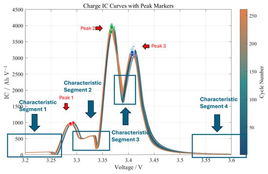
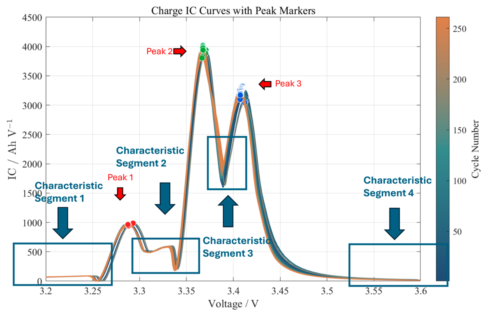
Based on the above analysis, the selection principles for the four voltage segments as features are as follows: the voltage variation values within a certain time duration after the start of discharge, before the end of discharge, and at the junctions of the two voltage plateaus during the discharge process. The positions of these segments are shown in Figure 1.
Figure 1.
Charging Incremental Capacity (IC) Curves.
Among them, the positions of the voltage plateau junctions can be determined by plotting the incremental capacity (IC) curves. Mathematically, the IC is defined as the derivative of capacity () with respect to voltage (), which can be explicitly expressed as:
As shown in Figure 1, the peak positions in the IC curves generally correspond to the voltage plateaus, and the required positions of the plateau junctions can be obtained from the voltages corresponding to the valleys in the IC curves. In the discharge curve of a single cycle, the positions of the voltage plateau junctions can be located by matching the voltages corresponding to the valleys of the IC curve.
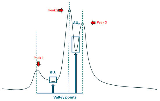
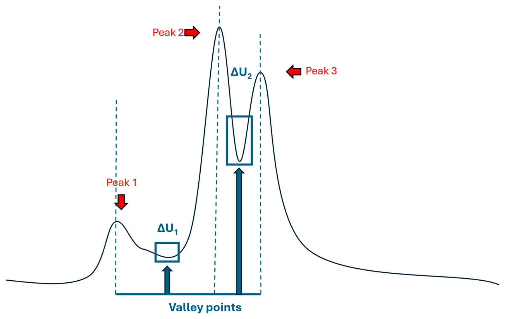
The specific calculation method for the voltage drop values is defined as follows: is the voltage difference between the voltage at the start of discharge and the voltage after seconds; is the voltage difference between the voltage seconds before the end of discharge and the voltage at the end of discharge; and are the voltage differences obtained by taking points s before and after the central point, which corresponds to the valley voltage of the IC curve in the discharge curve. To clarify, these “valley points” are exactly the local minima located between the characteristic peaks in the IC curve. Specifically, the first valley point is the local minimum between Peak 1 and Peak 2, and the second valley point is the local minimum between Peak 2 and Peak 3. To provide a more intuitive illustration of these definitions, a detailed schematic drawing based on a single IC curve is presented in Figure 2.
Figure 2.
Schematic diagram of the feature parameter extraction, illustrating the locations of , , and the corresponding valley points (local minima).
Taking at the start of discharge as an example, the calculation formula is as follows:
where is the voltage value at the 0th second, i.e., the start of discharge, and is the voltage value at the a-th second.
The calculation formula for the feature value SVF is as follows:
where represents the voltage difference at the start of discharge, represents the voltage difference at the end of discharge, and and represent the voltage differences near the first valley point and the second valley point of the IC curve, respectively. Theoretically, relying on a single voltage segment may only capture a partial degradation mechanism (e.g., purely ohmic resistance increase or specific phase-transition distortion). By comprehensively integrating the start, middle, and end segments, the proposed SVF incorporates multi-regime physical behaviors, ensuring feature complementarity. The detailed quantitative validation regarding the feature sensitivity and optimality using experimental datasets will be thoroughly demonstrated in Section 4.1.
2.2. Establishment of the Relationship Between SVF and Capacity
The Support Vector Machine (SVM) exhibits excellent performance in establishing the relationship between two variables for regression problems, enabling accurate fitting and further prediction. In this work, given the health indicator SVF, it is necessary to establish the mapping relationship between battery capacity and SVF, so that the corresponding capacity variation can be derived from the change in SVF.
Furthermore, the method proposed in this paper is mainly used for battery service life prediction, i.e., predicting the variation of State of Health (SOH). Therefore, after establishing the SVF-capacity relationship curve, it also needs to be extrapolated to enable the acquisition of the corresponding battery capacity once the predicted SVF values are obtained. The SVM method is adopted to fulfill the above requirements. The SVM fitting expression is as follows:
where are the Lagrange multipliers, is the kernel function, are the support vectors, and b is the bias term determined via training and fitting.
2.3. Establishment of the Relationship Between SVF and Cycle Number
The core of predicting battery capacity degradation lies in predicting the variation of SVF. The method proposed in this paper adopts a numerical fitting approach to fit the curve and predict its variation trend, and the natural logarithmic curve is specifically used for fitting here. Due to the inevitable errors inherent in numerical fitting methods, this paper combines Gaussian Process Regression (GPR) to perform residual correction on the fitting results. Meanwhile, the GPR correction algorithm enables the model to output results with probabilistic information, and confidence interval information can be obtained as required. This feature is more in line with the practical industrial application requirements.
The specific logarithmic fitting formula used here is as follows:
where the unknown parameters and are obtained by fitting the known SVF variation curve, and represents the number of battery cycles.
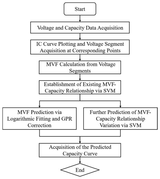
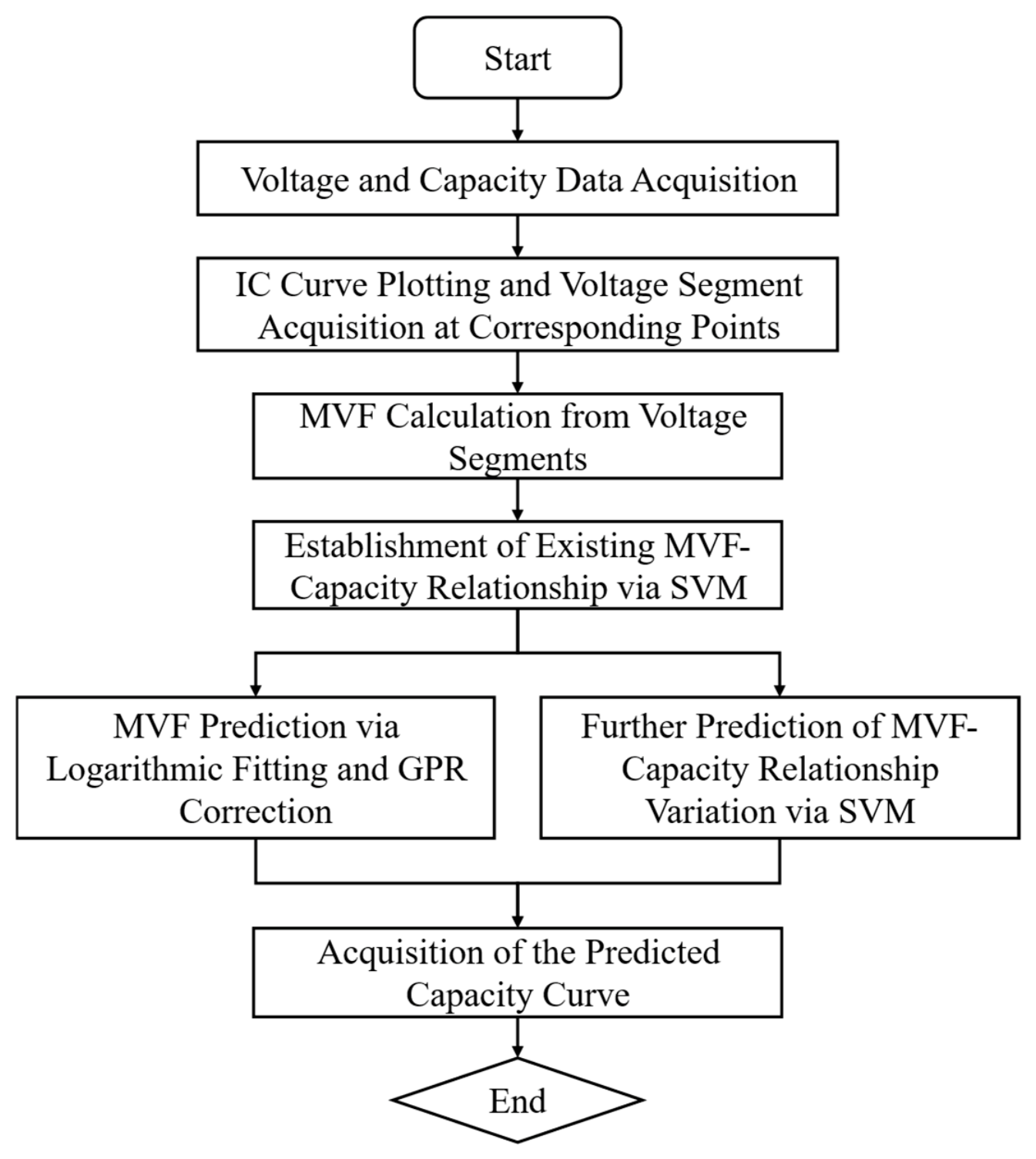
After the above SVF prediction is completed, the corresponding capacity prediction values are obtained through the mapping relationship described in Section 2.2 to complete the battery capacity prediction. The flowchart illustrating the implementation of this method is shown in Figure 3.
Figure 3.
Flowchart of the Proposed SVM-Numerical Fitting Method.
3. Arrhenius Hybrid Model Method
The hybrid model mainly consists of two components: the first part is the feedforward prediction of battery capacity based on the Arrhenius empirical model, and the second part is the feedback fusion correction based on data-driven methods. Together, they form a closed-loop hybrid capacity prediction model via the Kalman Filter. This model possesses online prediction correction capability and can realize the function of simultaneous online prediction and correction based on the acquired data, thereby achieving the effect that the prediction accuracy gradually improves as the volume of available data increases.
3.1. Arrhenius Feedforward Prediction Model
The Arrhenius model is an empirical model that takes temperature as the acceleration stress and the thickening of the negative Solid Electrolyte Interphase (SEI) film as the main capacity degradation mechanism. It generally achieves relatively good prediction performance under steady-state conditions [24]. The specific formula is as follows:
where A is the frequency factor, which represents the effective collision frequency of reactant molecules per unit time and reflects the initial rate of battery capacity degradation. is a combined term where is the activation energy and is the universal gas constant; this term reflects the degree of influence of activation energy on the reaction rate. is the compensation factor, which comprehensively represents the influence of other factors on the reaction. However, in practical applications, battery cycling is often performed under variable temperature operating conditions, and the acquired data are discrete points. To facilitate matrix calculation, it is necessary to discretize the Arrhenius formula to adapt to variable temperature conditions. The discretized formula is as follows:
where . The degradation of battery capacity with the number of cycles can be obtained through the iterative formula, thereby deriving the trend of battery capacity change.
Even after the above processing, since the Arrhenius model is an open-loop model, it is still prone to parameter mismatch during the iterative calculation process, resulting in an increasing deviation between the predicted results and the actual measured values. Therefore, it is necessary to use an online capacity estimation method to correct it in real time, so as to prevent the deviation from increasing and improve the prediction performance.
3.2. Online Capacity Estimation Method
For online capacity estimation, multiple approaches are available while adhering to the requirement of low computational complexity. Commonly used methods include the Ampere-hour integral method, State of Charge (SOC)-Open Circuit Voltage (OCV) look-up table method, among which the Ampere-hour integral method is adopted in this work.
The Ampere-hour integral method is the most widely used capacity estimation method at present, which calculates the battery capacity by integrating the charging/discharging current over time. It features relatively high estimation accuracy; however, its inherent drawback is that cumulative errors will inevitably accumulate with the extension of operation time, which seriously compromises the estimation accuracy and thus requires periodic calibration to eliminate. The specific calculation formula is as follows:
In this paper, this method is mainly applied to full charge–full discharge operating conditions, where the battery capacity can be calibrated at each complete charge and discharge cycle. Therefore, the cumulative error will not significantly degrade the performance of online estimation to a large extent.
3.3. Closed-Loop Model Fusion
The Kalman Filter (KF) is an optimal recursive state estimation algorithm based on the linear minimum mean square error (LMMSE) criterion, and it ranks among the most widely used classical methods in the fields of dynamic system state tracking and multi-source data fusion.
This algorithm adopts Bayesian estimation theory as its core framework, and realizes real-time optimal estimation of unknown state variables of dynamic systems through a closed-loop recursive iterative structure consisting of two core stages: prediction and update. Its core mechanism is elaborated as follows: in scenarios where both the a priori estimated value of the system and the real-time observed value contain random noise, and an unbiased true value is unavailable, the Kalman Filter can adaptively adjust the weight allocation between the a priori estimated value and the real-time observed value by quantifying the statistical characteristics of system process noise and measurement noise, thereby completing the optimal fusion solution of the state variable, rather than relying absolutely on a single data source.
Compared with conventional static data processing methods, the Kalman Filter has two core superiorities. First, its recursive operation structure eliminates the need to store full historical data and can complete iterative updates only with the state estimation result of the previous moment and the observation data of the current moment, which is inherently suitable for online real-time processing scenarios. Second, this method can effectively suppress the fluctuation of state estimation caused by system model deviation and random measurement noise. Furthermore, with the continuous accumulation of valid observation data during the iterative process, the state estimation result will gradually converge to the true value of the system, with continuously improved estimation accuracy and stability.
In the battery capacity degradation and Remaining Useful Life (RUL) prediction framework constructed in this paper, we define the predicted battery capacity calculated based on the Arrhenius aging model as the a priori state estimate in the state equation of the Kalman Filter. Meanwhile, the estimated battery capacity obtained by online real-time calculation via the Ampere-hour integral method (i.e., Coulomb counting method, the universal term in international battery research) is defined as the real-time measurement value in the measurement equation of the Kalman Filter. Through the recursive iterative structure of the Kalman Filter, real-time optimal fusion of the above two sets of capacity estimation results is implemented. Ultimately, online dynamic correction during the long-term prediction of battery capacity is achieved, and the closed-loop estimation effect of “simultaneous prediction and correction” is accomplished, which effectively improves the accuracy and robustness of battery capacity and RUL prediction results.
4. Method Validation and Comparative Analysis
In this paper, the voltage and current data of 281 cycles from one 320 Ah high-capacity lithium iron phosphate (LFP) battery cell in an energy storage system is used as the data source for validating the two proposed methods. Furthermore, another single 298 Ah large-scale LFP battery cell is employed for further validation of the proposed methods. Table 1 presents the detailed cyclic aging test conditions:
Table 1.
Experimental Conditions for Cyclic Aging Tests.
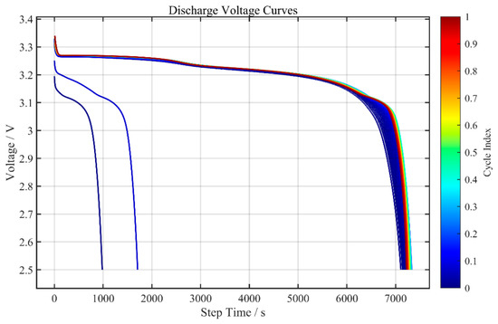
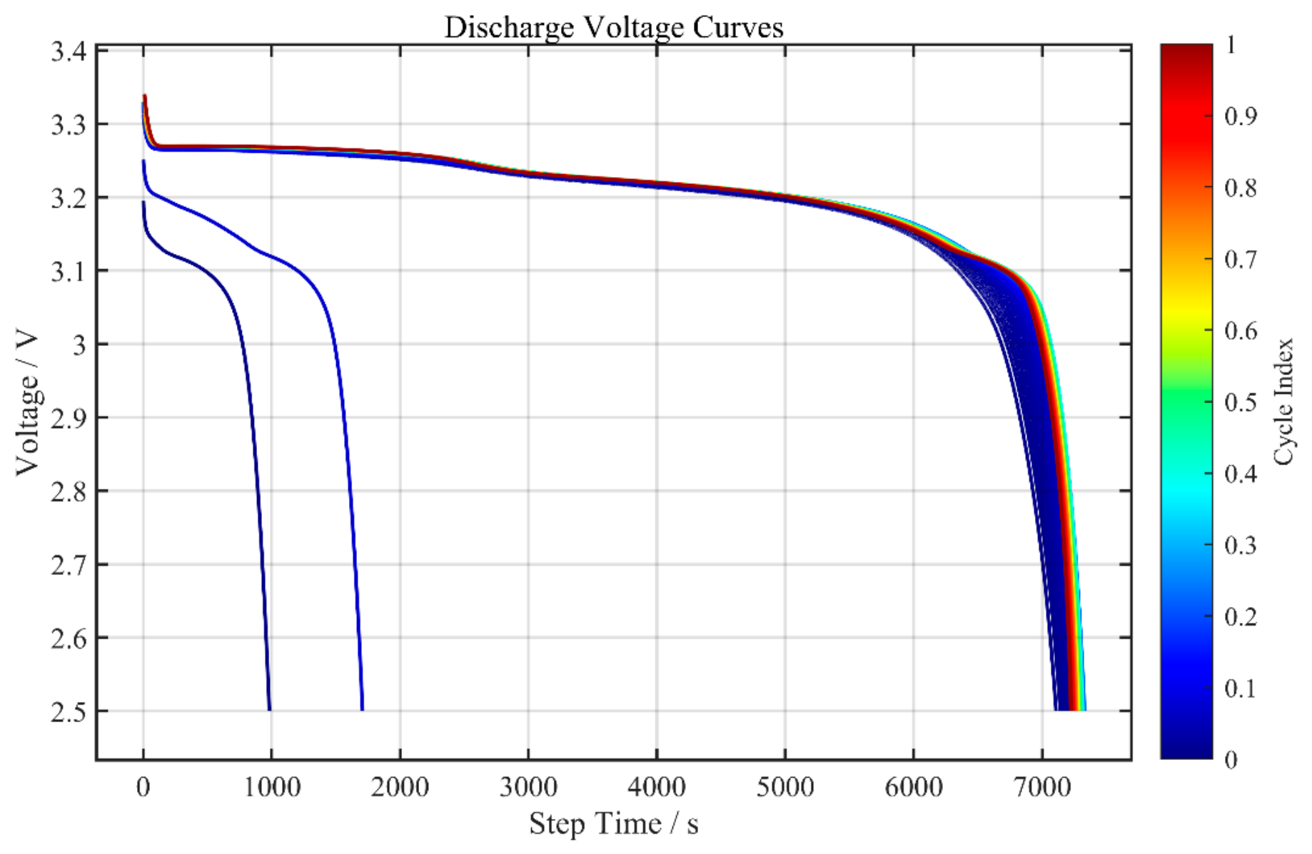
Since the cells used in the experiments are pristine cells, it is speculated that issues such as incomplete electrolyte wetting exist, leading to an initial capacity rise phenomenon during the early stage of cyclic aging. The corresponding discharge curves are shown in Figure 4. To prevent abnormal data caused by the initial capacity rise and test condition fluctuations from compromising the model performance, data cleaning was performed to remove the cycle data corresponding to the capacity rise phase and abnormal operating states.
Figure 4.
Discharge Voltage Curves.
4.1. Validation of the SVM-Numerical Fitting Method
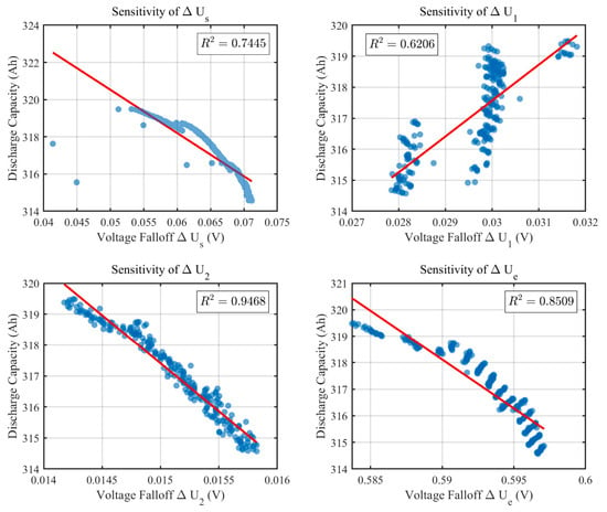
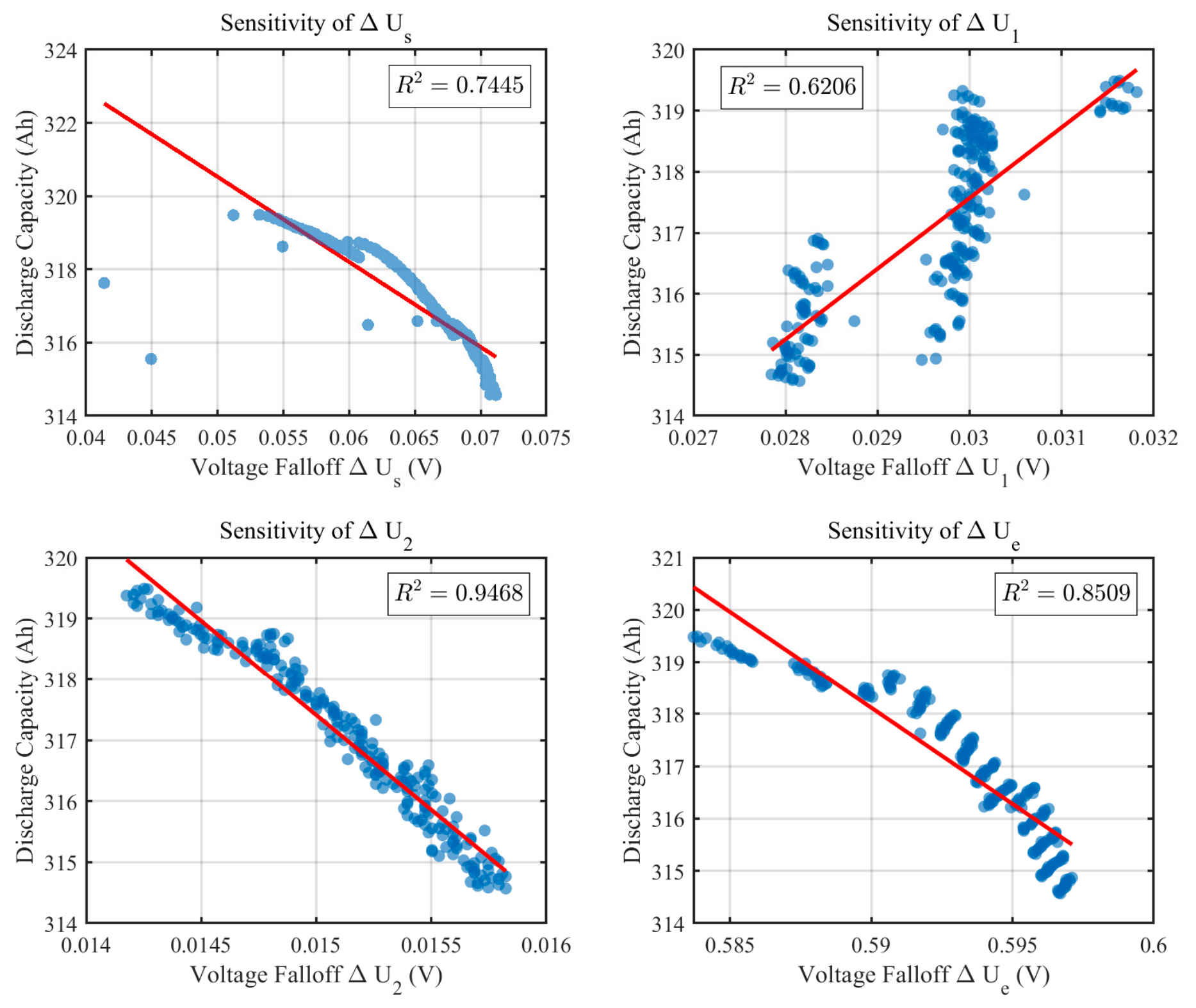
First, feeding the extracted features into the predictive models, a feature sensitivity and ablation study was conducted to quantitatively evaluate the correlation and optimality of the selected voltage segments. The quantitative relationships between different feature combinations and the actual battery capacity were analyzed using the Pearson correlation coefficient () and the coefficient of determination (). The results based on the experimental dataset are summarized in Table 2.
Table 2.
Feature ablation study: Correlation analysis of different voltage segment combinations with actual discharge capacity.
As indicated, Combination 1 (), which predominantly represents the ohmic internal resistance and end-stage polarization, exhibits the highest linear correlation (). In contrast, Combination 2 (), representing the phase-transition regimes, shows a moderate positive correlation (), highlighting a non-linear evolutionary behavior characteristic of LFP battery aging dynamics.
When all four segments are integrated into the proposed SVF (Combination 3), a strong global correlation is maintained (). The correlation analysis results of the four parameters are presented in Figure 5. It is worth noting that although the purely linear fit of Combination 3 is slightly diluted compared to Combination 1 due to the algebraic summation of multi-regime behaviors (linear and non-linear), the inclusion of the mid-segments is physically and methodologically essential. Because the subsequent life prediction relies on a non-linear machine learning model (SVM, as discussed in Section 2), the integration of all four segments introduces indispensable non-linear domain knowledge (phase-transition distortion). This feature complementarity prevents the model from overfitting to a single degradation symptom (e.g., ohmic drop) and significantly enhances the global prediction robustness.
Figure 5.
Feature sensitivity analysis: Scatter plots and linear regression fitting results between the four individual extracted voltage drop segments (, , , ) and the actual discharge capacity.
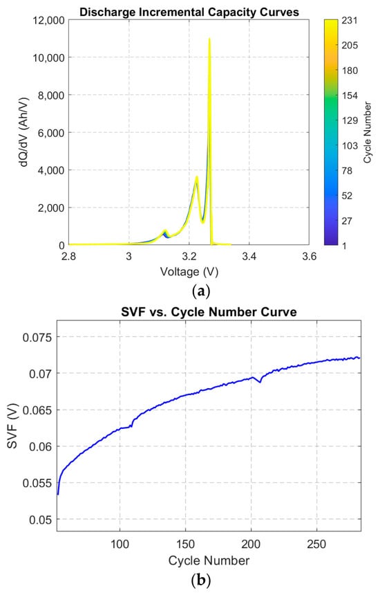
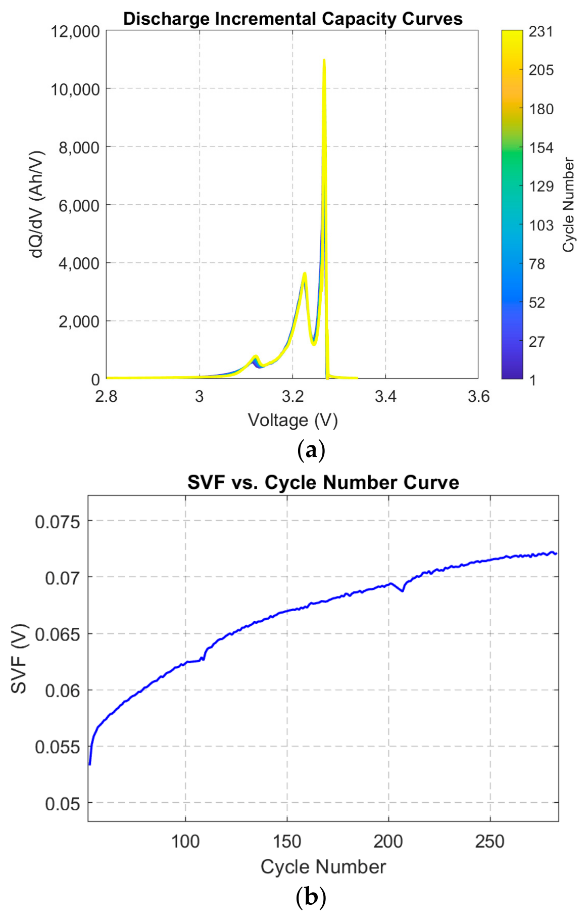
The incremental capacity (IC) curves were plotted using the discharge voltage data as shown in Figure 6a. The peaks and corresponding valleys were extracted, and the required voltage drop values at the corresponding positions were obtained to derive the SVF. The SVF versus cycle number plot is presented in Figure 6b.
Figure 6.
(a) Discharge Incremental Capacity (IC) Curves; (b) SVF versus Cycle Number Curve.
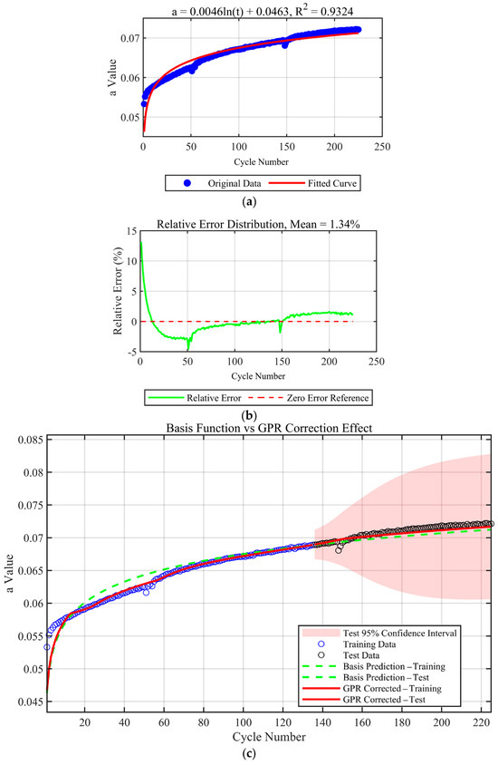
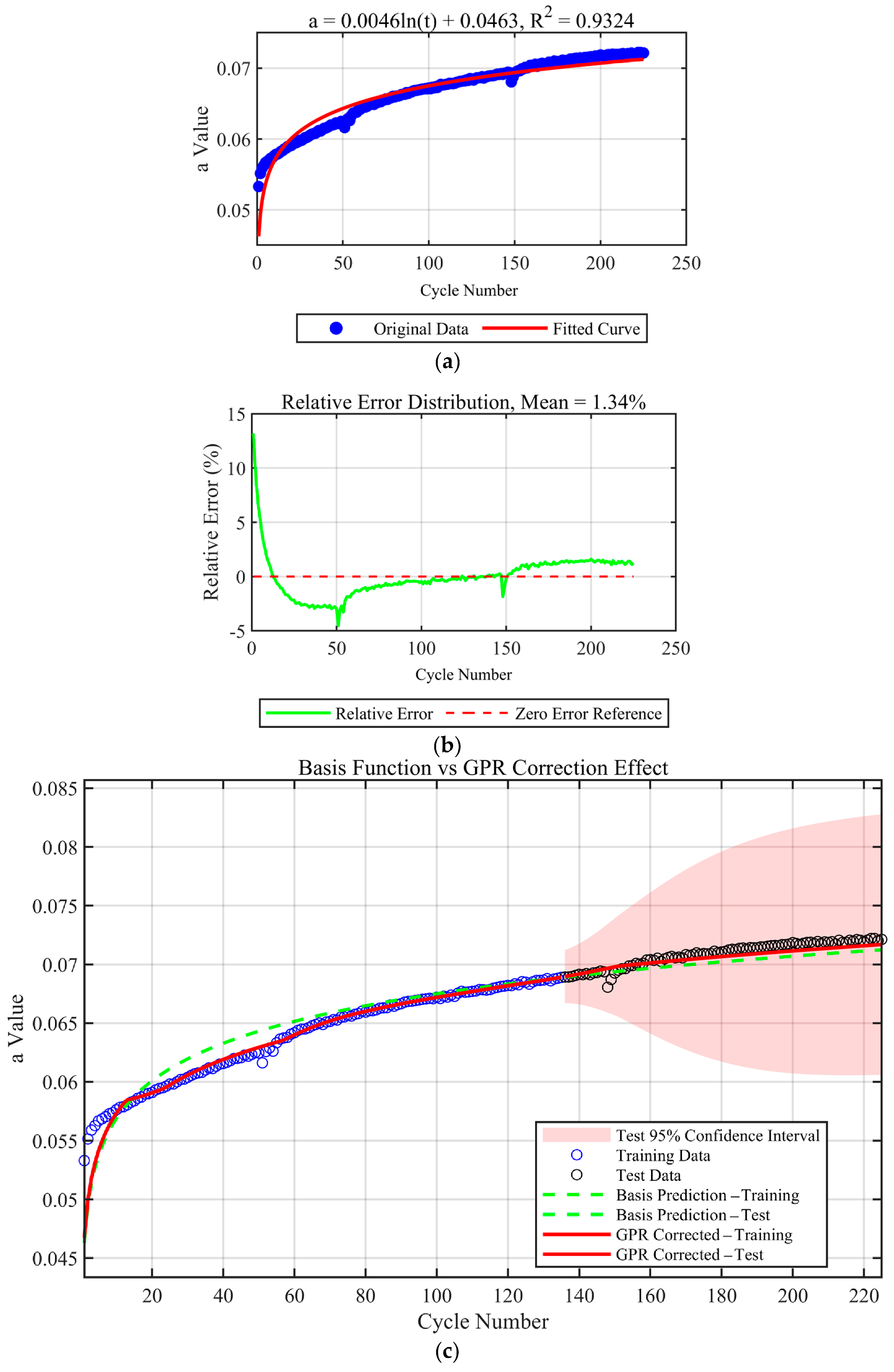
Subsequently, the variation trend of SVF was fitted and predicted. As can be observed from the curve in Figure 6b, its variation trend resembles a natural logarithmic curve. It is worth noting that there are two distinct “bumps” (abnormal fluctuations) at around the 110th and 210th cycles in Figure 6b, which is plotted using the raw data. These fluctuations are attributed to the specific aging test protocol, where the batteries were cycled in groups of 100 cycles, followed by prolonged rest periods. The extended resting phases allow the battery to undergo capacity recovery and parameter relaxation, leading to these temporary spikes in the measured data. Similarity analysis yields a Pearson correlation coefficient of 0.9907 between the two. Therefore, the natural logarithmic fitting method is appropriate for this scenario. Prior to model training, a data cleaning process was conducted to remove certain outlier data points to prevent these severe anomalies from negatively affecting the algorithm’s performance. As a result of removing these irregular cycles, the data sequence was compressed. The fitting effect on the cleaned dataset is shown in Figure 7a, with an obtained R2 value of 0.9324. Consequently, the aforementioned “bumps” originally located at the 110th and 210th cycles in Figure 6b are shifted to approximately the 50th and 150th cycles in Figure 7a,b. Moreover, the relative error distribution shown in Figure 7b indicates that the error is only large at the initial cycles and then decreases rapidly to maintain a low level.
Figure 7.
Result of the model. (a) Logarithmic Curve Fitting Result of SVF; (b) Relative Error Distribution of Logarithmic Fitting; (c) Validation Result of the GPR-Corrected Logarithmic Fitting Model.
To further eliminate the fitting error, the Gaussian Process Regression (GPR) model was adopted for residual correction. To verify the fitting and prediction performance, the dataset was divided into a 60% training set and a 40% test set. The results are shown in Figure 7c, which demonstrates that the data obtained after GPR correction is closer to the actual measured data. For the validation set, since no new data is introduced, the correction term of the GPR model will quickly reach an equilibrium state, which sufficiently demonstrates the effectiveness of the proposed model.
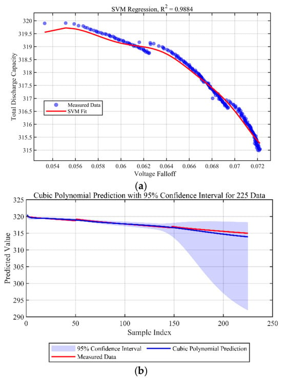
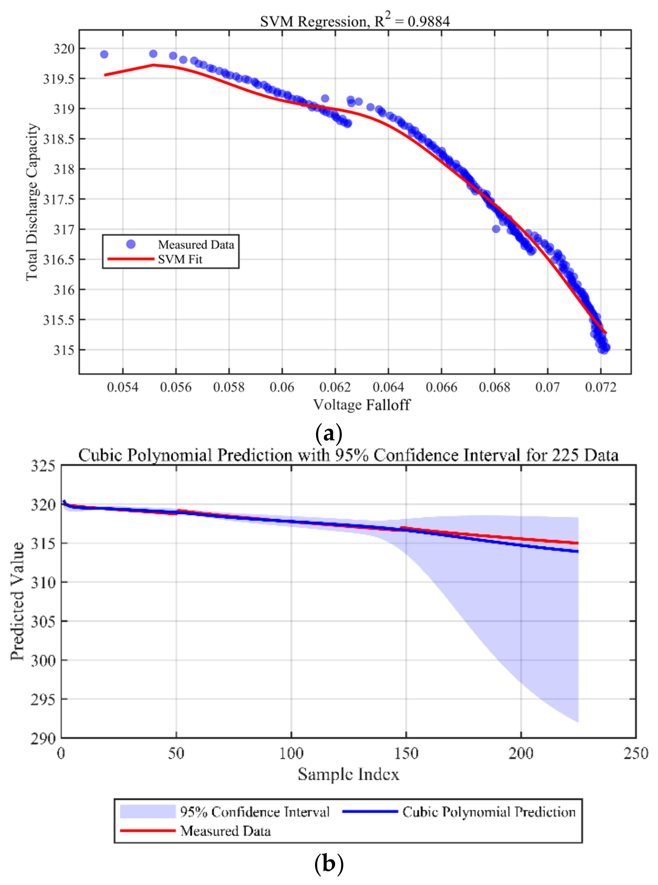
Next, the relationship between SVF and battery capacity was established, and the SVF versus battery capacity curve was plotted. The SVM method was used to fit and predict the curve as shown in Figure 8a, which exhibits a good fitting effect for the data points with an R2 value of 0.9886. Based on the obtained relationship curve, the fitted and predicted SVF curves were converted to capacity degradation, and the corresponding confidence intervals were output simultaneously. Figure 8b presents the final prediction results including both the training set and the test set.
Figure 8.
(a) Discharged Battery Capacity vs. SVF; (b) Capacity Prediction Result of the SVM-Numerical Fitting Method.
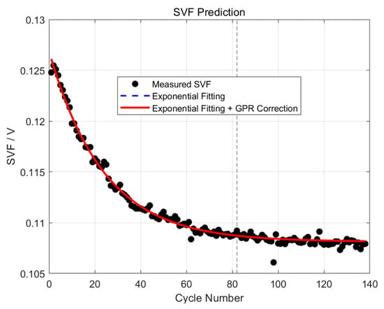
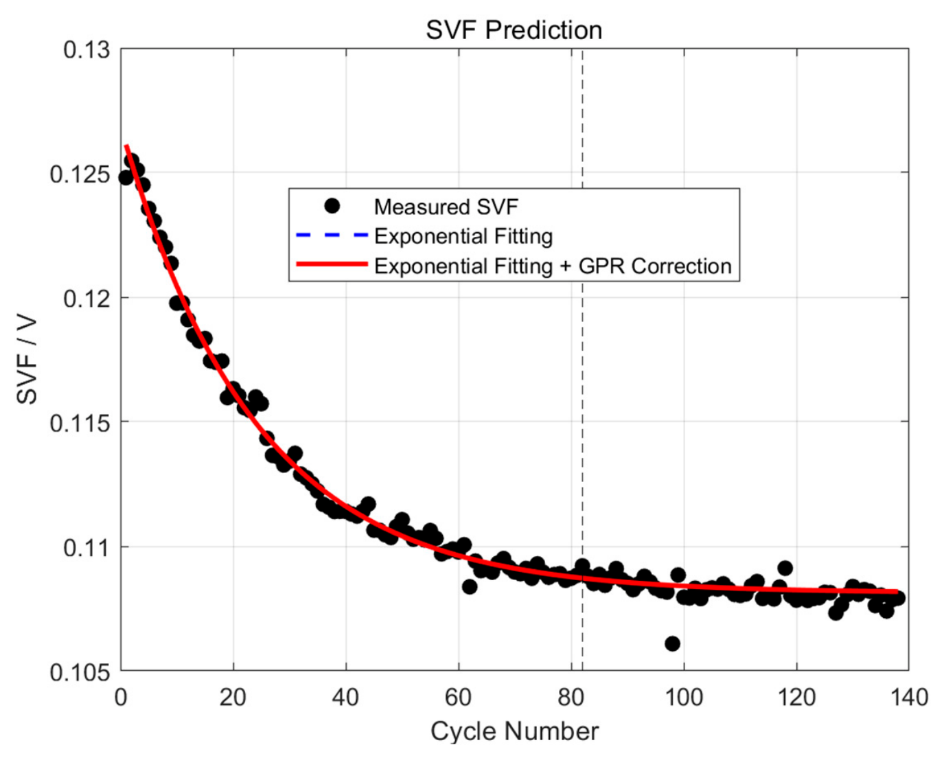
Further validation was conducted on large-capacity lithium iron phosphate (LFP) batteries with a nominal capacity of 298 Ah. A total of 150 cycles of cyclic aging data were collected, and the voltage drop SVF was calculated after data cleaning. Based on the SVF results, the variation trend of SVF with cycle number was fitted using the combination of logarithmic fitting and Gaussian Process Regression (GPR) residual correction. The dataset was also divided into a 60% training set and a 40% test set to demonstrate the effectiveness of the proposed method. The SVF variation with cycle number and the corresponding fitting and prediction results are presented in Figure 9.
Figure 9.
Exponential curve fitting (298 Ah).
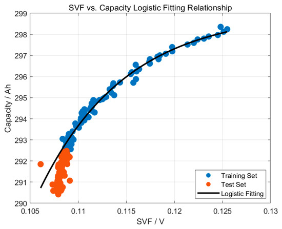
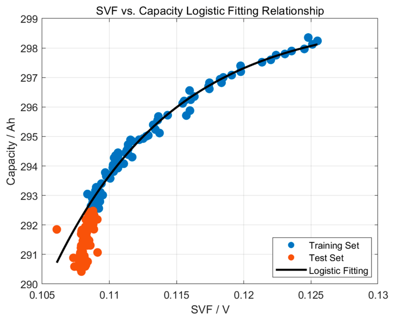
As can be observed from the figure, the adopted method of exponential fitting combined with GPR correction can achieve excellent fitting performance for the SVF variation trend and exhibits satisfactory performance even in the test set. Subsequently, the exponential function was used to establish the relationship between SVF and battery capacity degradation, and the data fitting and prediction were completed. The results are shown in Figure 10.
Figure 10.
Battery Capacity Curve versus SVF (298 Ah).
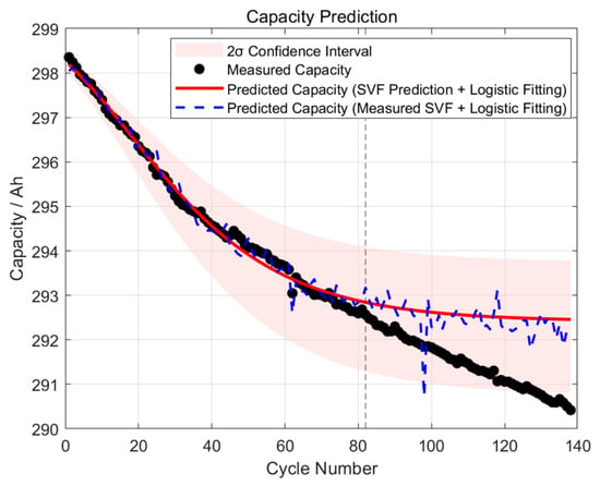
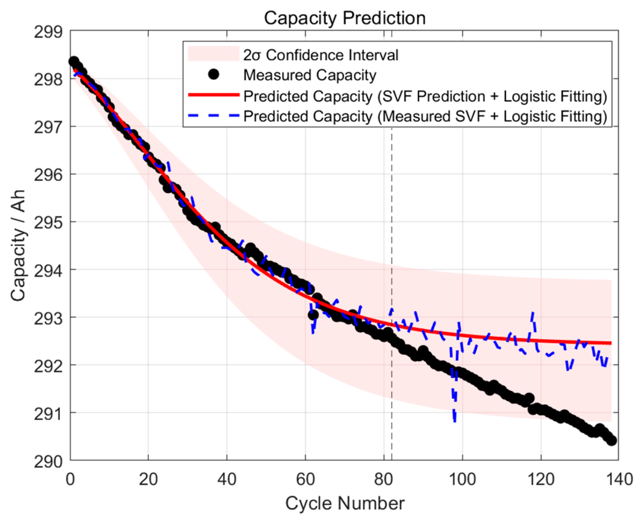
It can be seen from the figure that the adopted Logistic function can also well capture the variation trend of the SVF-capacity relationship and accurately predict the subsequent trend. Finally, the final capacity degradation curve fitting and subsequent degradation prediction results obtained by combining the above methods are presented in Figure 10. It is important to clarify that the vertical dashed line in Figure 11 delineates the boundary between the training set and the test set. As observed, the fitting performs excellently in the training phase, but a certain degree of trend divergence appears beyond the dashed line (after approximately 80 cycles). This deviation is primarily attributed to the combined effects of local data outliers and the relatively limited volume of training data. Given that fewer than 300 cycles constitute merely a minute fraction of the entire lifecycle of a 300 Ah large-scale energy storage battery, achieving a perfectly fitted long-term trajectory with limited early-stage data is highly challenging. Nevertheless, the overall predicted curve still conforms to the actual physical degradation process, which demonstrates that the proposed method can also relatively well capture the capacity variation trend.
Figure 11.
Capacity Prediction Result of the Logistic-Numerical Fitting Method.
4.2. Validation of the Hybrid Model Method
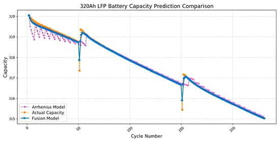
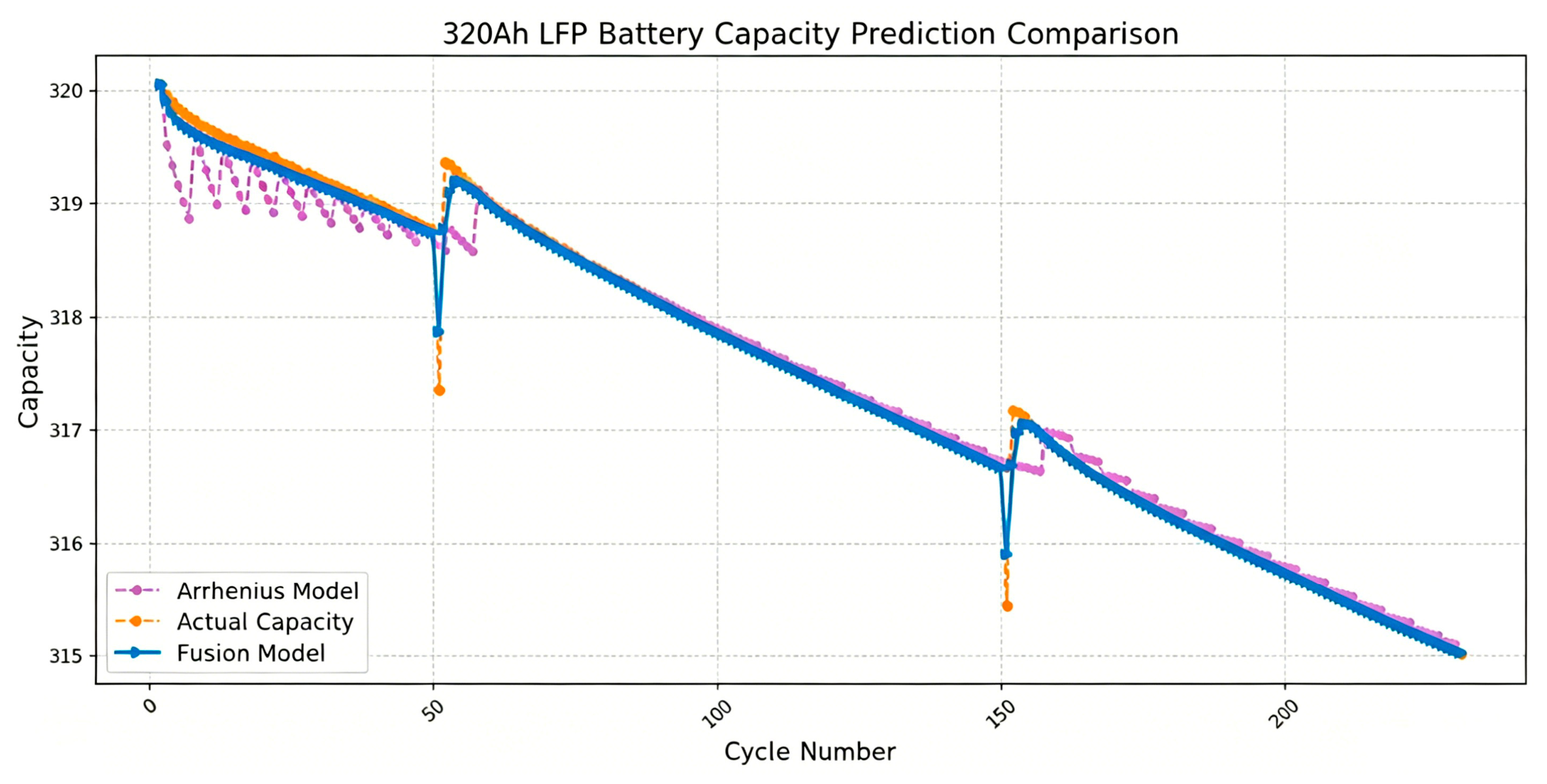
For the normal cyclic aging data corresponding to the capacity degradation phase, capacity estimates were iteratively obtained using the discretized Arrhenius model, while online capacity measurement values were derived via the Ampere-hour integral method. The parameter update frequency for the Arrhenius model was set to once every 5 cycles, and the model fusion weight was set to 0.5, meaning the model assigned equal confidence levels to the estimated values and the measured values at this stage.
The obtained results are shown in Figure 12. It can be observed that as the number of cycles increases, the parameters of the Arrhenius model are gradually calibrated, causing its estimated values to progressively converge to the measured values. After 60 cycles, the results generated by the standalone Arrhenius model are already in good agreement with the actual measured results; however, non-negligible residual errors still exist. In contrast, the results obtained by the hybrid model can effectively compensate for these residual errors, eliminate spurious fluctuations, and achieve the desired effect of simultaneous prediction and correction.
Figure 12.
Test Result of the Arrhenius Hybrid Model.
4.3. Method Comparison
In summary, the SVM-Numerical Fitting Method proposed in this paper is characterized by lower data requirements compared with the hybrid model method. The required SVF is derived from the voltage variation segments at four positions; thus it does not require complete voltage curves. However, due to its inherent requirement for real-time observation values, the Ampere-hour integral capacity estimation method adopted under the data conditions used in this paper necessitates complete voltage and current time-series curves.
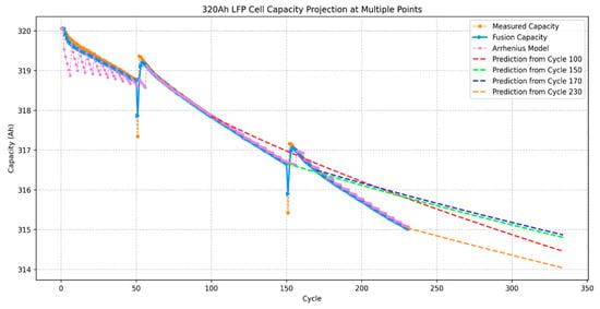
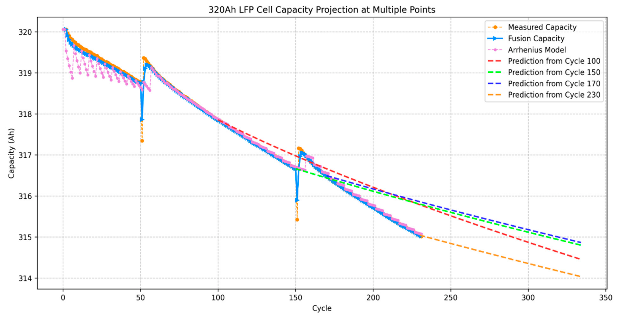
Comparing the life prediction results obtained by the two methods, the results of the SVM-Numerical Fitting Method are shown in Figure 8b, and those of the Arrhenius Hybrid Model Method are presented in Figure 13. It can be seen that under the current experimental conditions, with the identical dataset partition strategy, the results obtained by the former are relatively closer to the test data and exhibit smaller prediction errors than the latter. In addition, according to the output confidence interval data, with 80% capacity retention defined as the end-of-life (EOL) criterion, the worst-case cycle life reaches 3004 cycles within the 2σ range commonly used in industrial scenarios, and 884 cycles within the 3σ range.
Figure 13.
Long-Term Capacity Prediction Result of the Arrhenius Hybrid Model.
On the other hand, as an offline life prediction approach, the former requires a complete recalculation of the entire model to obtain updated results as the volume of subsequent operational data increases. In contrast, the latter functions as an online life prediction method, where its model parameters are continuously adjusted adaptively as more data accumulates. As evident from Figure 13, the life prediction results differ significantly when performed with different amounts of accumulated data; accumulating more operational data consistently yields more accurate prediction results in the hybrid model, which represents a distinct foreseeable advantage of the latter for long-term field applications.
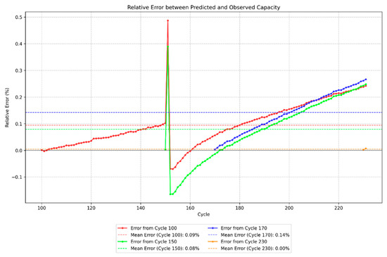
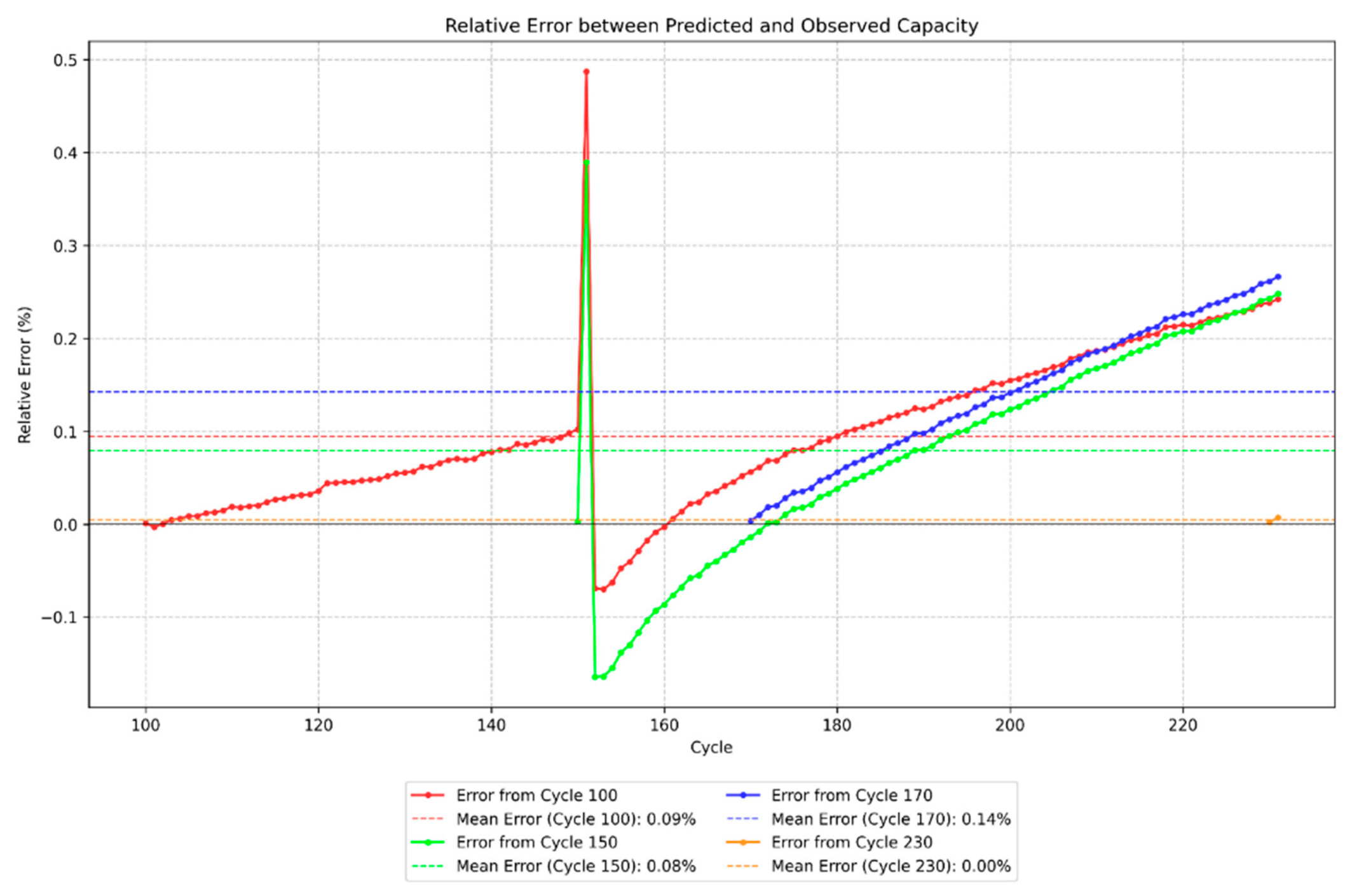
Under the current test conditions, the relative error of the standalone Arrhenius model after correction does not exceed 1%, and the error evolution of the hybrid model is illustrated in Figure 14. By reasonably extrapolating the observed relative error variation trend, the Arrhenius-based hybrid model can reliably predict the capacity degradation for approximately the next 1000 charge–discharge cycles within a 5% relative error tolerance. In comparison, as a purely data-driven offline prediction method, the long-term extrapolation error of the SVM-Numerical Fitting Method is more difficult to quantify and bound in advance.
Figure 14.
Relative Error Evolution of the Arrhenius Hybrid Model.
Finally, it must be frankly acknowledged that while this study provides EOL estimates based on the proposed models, the actual full-lifecycle EOL data is currently unavailable for direct validation. This absence is a foreseen limitation, primarily dictated by the practical constraints of industrial applications. The tested objects are 300+ Ah large-capacity LFP energy storage batteries, which inherently possess an extremely long cycle life. Conducting a complete, continuous cycle-to-death aging experiment for such large-scale cells is highly time-consuming and cost-prohibitive in the short term. Consequently, validating the exact long-term accuracy of these EOL predictions remains a foreseeable challenge. Future research will focus on continuously tracking the operational data of these deployed energy storage systems over an extended period to eventually acquire actual EOL data, which will be utilized to systematically verify and further refine the proposed prediction models.
5. Conclusions
To address the challenge of difficulty in acquiring complete voltage curve data during battery cycling, this paper proposes two battery life prediction methods belonging to the data-driven category and the empirical-data hybrid-driven category, respectively. The life prediction performance of both methods is verified using cyclic aging data of high-capacity lithium iron phosphate (LFP) cells from an actual energy storage system, and the data-driven method is further validated using an additional batch of cyclic aging data from large-capacity LFP batteries. Comparative results show that the data-driven SVM-Numerical Fitting Method achieves relatively higher accuracy when the available data volume is limited and can accurately fit the actual measured data. In contrast, the Arrhenius Hybrid Model exhibits inferior performance compared with the former method under limited data conditions; however, it outperforms the former method in terms of accuracy when more data is available and the model parameters are iteratively updated multiple times.
Based on the above research conclusions, for large-capacity energy storage systems, the online hybrid model is more suitable for continuous Remaining Useful Life (RUL) monitoring during long-term operation, and its accuracy gradually improves as the system operation time increases. In contrast, the offline data-driven model is more applicable for standalone one-time inspections or scenarios where the system operation data volume is relatively small. Notably, the technical route of extracting degradation features from partial voltage segments to get rid of the dependence on complete charge–discharge curves has been widely verified in recent relevant studies. For instance, Zhang et al. [25] proposed a model cluster framework adapting to different lengths of charging voltage segments for battery capacity estimation. This method builds multiple submodels corresponding to voltage segments of different positions and widths, and achieves a maximum root mean square error of only 0.403% under simulated real charging scenarios, fully confirming the rationality and engineering application value of the segmentation-based feature extraction method adopted in this paper. It also indicates that the life prediction methods proposed in this work have broad application prospects in actual energy storage scenarios with incomplete operating data. Overall, the two proposed methods have their own advantages and disadvantages and can exert their respective strengths according to different application scenarios.
In this paper, the number of cycles of the data used for method validation is less than 300, which is still far from the end-of-life (EOL) for high-capacity LFP cells. Furthermore, as large-capacity cells, their degradation characteristics differ from those of commonly used relatively small-capacity cells. Therefore, even though two batches of data were used for method validation, the obtained validation results still have certain limitations, and the applicability of the proposed methods needs further exploration. In addition, the respective advantages and disadvantages of the two methods mentioned in the above conclusions can be further optimized to minimize their shortcomings and maximize their strengths.
Author Contributions
Conceptualization, C.W. and H.Z.; Methodology, S.L. and G.Z.; Validation, M.J., P.G. and K.J.; Formal analysis, H.M., Y.Z. (Yong Zang), Y.Z. (Yingmeng Zhang) and G.S.; Investigation, S.L. and G.Z.; Data curation, H.M., Y.Z. (Yong Zang), Y.Z. (Yingmeng Zhang) and G.S.; Writing—original draft, H.L., G.H. and Q.H.; Writing—review and editing, H.L., G.H., C.W. and H.Z.; Visualization, M.J., P.G. and K.J.; Project administration, Q.H., H.L. and G.H. contributed equally to this work. All authors have read and agreed to the published version of the manuscript.
Funding
This work was supported by the Science and Technology Project of China Southern Power Grid Co., Ltd. [000000KC24040098], [ZBKJXM20240189].
Data Availability Statement
The original contributions presented in this study are included in the article. Further inquiries can be directed to the corresponding authors.
Acknowledgments
The authors would like to thank the support of the experimental platform and all members of the research team.
Conflicts of Interest
Authors Hao Liu, Guozhi Huang, Shijie Li, Guobin Zhong, Chao Wang were employed by the company China Southern Power Grid. The remaining authors declare that the research was conducted in the absence of any commercial or financial relationships that could be construed as a potential conflict of interest.
Abbreviations
The following abbreviations are used in this manuscript:
| SVM | Support Vector Machine |
| LSTM | Long Short-Term Memory |
| CNN | Convolutional Neural Network |
| GRU | Gated Recurrent Unit |
| P2D | Pseudo Two-Dimensional |
| RUL | Remaining Useful Life |
| SOH | State of Health |
| SOC | State of Charge |
| SEI | Solid Electrolyte Interphase |
| ECM | Equivalent Circuit Model |
References
- Wei, W. Characteristics and Optimization of the Battery Energy Storage System in the Renewable Energy Grid-Connected System. Ph.D thesis, Shandong University, Jinan, China, 2022. [Google Scholar] [CrossRef]
- Sun, T.; Kong, Y.; Qiao, D.; Guo, Y.; Li, X.; Li, D.; Zhao, Z.; Dai, H.; Li, L.; Wu, Y.; et al. A Novel Multi-Fault Diagnosis Method for Lithium-Ion Batteries Based on Cloud Low-Density Segment Charging Voltage Curves. IEEE Trans. Transp. Electrif. 2026, 12, 5243–5254. [Google Scholar] [CrossRef] [Scilit]
- Xiong, R.; Zhu, Y.; Zhang, Q.; Zhang, K.; Mei, B.; Sun, F. Review on Research Progress and Application of Low-temperature Heating Techniques for Lithium-ion Batteries. J. Mech. Eng. 2025, 61, 109–128. [Google Scholar] [CrossRef] [Scilit]
- Sun, T.; Wang, L.; Ren, D.; Shi, Z.; Chen, J.; Zheng, Y.; Feng, X.; Han, X.; Lu, L.; Wang, L.; et al. Thermal Runaway Characteristics and Modeling of LiFePO4 Power Battery for Electric Vehicles. Automot. Innov. 2023, 6, 414–424. [Google Scholar] [CrossRef] [Scilit]
- Gu, J.P.; Jiang, L.; Zhang, X.S.; Hua, L.; Cheng, T.Y. Estimation and Influencing Factor Analysis of Lithium-Ion Batteries State of Health Based on Feature Extraction. Trans. China Electrotech. Soc. 2023, 38, 5330–5342. [Google Scholar] [CrossRef]
- Schöberl, J.; Ank, M.; Schreiber, M.; Wassiliadis, N.; Lienkamp, M. Thermal runaway propagation in automotive lithium-ion batteries with NMC-811 and LFP cathodes: Safety requirements and impact on system integration. eTransportation 2024, 19, 100305. [Google Scholar] [CrossRef] [Scilit]
- Wang, Z.; Shi, D.; Zhao, J.; Chu, Z.; Guo, D.; Eze, C.; Qu, X.; Lian, Y.; Burke, A.F. Battery health diagnostics: Bridging the gap between academia and industry. eTransportation 2024, 19, 100309. [Google Scholar] [CrossRef] [Scilit]
- Peng, J.; Zhao, X.; Ma, J.; Meng, D.; Zhu, J.; Zhang, J.; Yan, S.; Zhang, K.; Han, Z. Enhancing lithium-ion battery monitoring: A critical review of diverse sensing approaches. eTransportation 2024, 22, 100360. [Google Scholar] [CrossRef] [Scilit]
- Han, X.; Lu, L.; Zheng, Y.; Feng, X.; Li, Z.; Li, J.; Ouyang, M. A review on the key issues of the lithium-ion battery degradation among the whole life cycle. eTransportation 2019, 1, 100005. [Google Scholar] [CrossRef] [Scilit]
- Guo, D.; Lu, T.; Sun, T.; Lai, X.; Han, X.; Zheng, Y. Facilitating battery quality classification: Early life prediction with sequence-sampling data augmentation. eTransportation 2026, 28, 100553. [Google Scholar] [CrossRef] [Scilit]
- Sun, T.; Wang, S.; Jiang, S.; Xu, B.; Han, X.; Lai, X.; Zheng, Y. A cloud-edge collaborative strategy for capacity prognostic of lithium-ion batteries based on dynamic weight allocation and machine learning. Energy 2022, 239, 122185. [Google Scholar] [CrossRef] [Scilit]
- Sun, T.; Wu, W.; Zhou, C.; Wang, X.; Cheng, C.; Lu, M.; Wang, T.; Xu, C.; Feng, X.; Shen, K.; et al. Variable Density Modeling of Lithium-Ion Battery Thermal Runaway Considering Mass Loss of Gas and Particles. Process. Saf. Environ. Prot. 2026, 211, 108842. [Google Scholar] [CrossRef] [Scilit]
- Hu, J.; Fu, P.; Hu, X.; Wei, Z.; Early, J.; Fly, A.; Zhang, Y.; Huang, Y. Toward advanced estimation of state of health for integral lithium-ion battery pack. Cell Rep. Phys. Sci. 2025, 6, 102363. [Google Scholar] [CrossRef] [Scilit]
- Zhou, Y.; Gu, H.; Su, T.; Han, X.; Lu, L.; Zheng, Y. Remaining useful life prediction with probability distribution for lithium-ion batteries based on edge and cloud collaborative computation. J. Energy Storage 2021, 44, 103342. [Google Scholar] [CrossRef] [Scilit]
- Kim, S.; Jun, H.; Lee, M.; Choi, Y.Y.; Choi, J.-I. Model-free reconstruction of capacity degradation trajectory of lithium-ion batteries using early cycle data. eTransportation 2023, 17, 100243. [Google Scholar] [CrossRef] [Scilit]
- Zhang, K.; Lv, T.; Chen, X.; Chen, J.; Shen, Y.; Zhou, L.; Sun, T.; Zheng, Y. Study on battery capacity recognition method for real electric vehicle under complex operating conditions. J. Energy Storage 2025, 118, 116219. [Google Scholar] [CrossRef] [Scilit]
- Zhang, L.; Su, X.; Zhang, C.; Wang, Y.; Wang, Y.; Zhu, T.; Fan, X. An Adaptable Capacity Estimation Method for Lithium-Ion Batteries Based on a Constructed Open Circuit Voltage Curve. Batteries 2025, 11, 265. [Google Scholar] [CrossRef] [Scilit]
- Sun, T.; Chen, J.; Wang, S.; Chen, Q.; Han, X.; Zheng, Y. Aging mechanism analysis and capacity estimation of lithium—Ion battery pack based on electric vehicle charging data. Energy 2023, 283, 128457. [Google Scholar] [CrossRef] [Scilit]
- Han, X.; Mao, S.; Wang, Y.; Lu, Y.; Wang, D.; Sun, Y.; Zheng, Y.; Feng, X.; Lu, L.; Hua, J.; et al. Manipulation of lithium dendrites based on electric field relaxation enabling safe and long-life lithium-ion batteries. Nat. Commun. 2025, 16, 3699. [Google Scholar] [CrossRef] [Scilit] [PubMed]
- Liang, H.Q.; He, H.W.; Dai, K.W.; Pang, B.; Wang, P. Research on Lithium Ion Battery Life Prediction Method Based on Empirical Aging Model and Mechanism Model for Electric Vehicles. Automot. Eng. 2023, 45, 825–835+844. [Google Scholar] [CrossRef]
- Wang, P.; Zhang, J.A.; Cheng, Z.; Yu, Y.X. Joint state estimation method of lithium-ion batteries based on charging voltage segments. J. Hunan Univ. (Nat. Sci.) 2021, 48, 187–200. [Google Scholar] [CrossRef]
- Sun, T.; Jiang, S.; Li, X.; Wang, X.; Ma, Y.; Zheng, Y. A Novel Capacity Estimation Approach for Lithium-Ion Batteries Combining Three-Parameter Capacity Fade Model With Constant Current Charging Curves. IEEE Trans. Energy Convers. 2021, 36, 2574–2584. [Google Scholar] [CrossRef] [Scilit]
- Tang, X.; Meng, X.; Liu, Z.; Miao, Y.; Hasanien, H.M.; Li, M.; Liu, J.; Sun, C. State of health estimation and degradation quantification of PEMFCs using a dynamic coupling method of data-driven and electrochemical impedance. IEEE Trans. Transp. Electrif. 2026, 12, 5761–5772. [Google Scholar] [CrossRef] [Scilit]
- Xi, R.; Mu, Z.; Ma, W.; Jin, W.; Ma, H.; Liu, K.; Li, J.; Yu, M.; Jin, D.; Cheng, F. Lifetime prediction of rechargeable lithium-ion battery using multi-physics and multiscale model. J. Power Sources 2024, 608, 234622. [Google Scholar] [CrossRef] [Scilit]
- Zhang, Q.; Zhu, J.; Wang, Y.; Wei, X.; Dai, H. A Model Cluster Adapting to Different Charge Voltage Segments for Battery Capacity Estimation. Automot. Innov. 2025, 8, 753–768. [Google Scholar] [CrossRef] [Scilit]

Disclaimer/Publisher’s Note: The statements, opinions and data contained in all publications are solely those of the individual author(s) and contributor(s) and not of MDPI and/or the editor(s). MDPI and/or the editor(s) disclaim responsibility for any injury to people or property resulting from any ideas, methods, instructions or products referred to in the content. |
© 2026 by the authors. Licensee MDPI, Basel, Switzerland. This article is an open access article distributed under the terms and conditions of the Creative Commons Attribution (CC BY) license.