BATWO: Bayesian Adaptive Time Window Optimization for Feature Extraction in SOH Estimation of Li-Ion Batteries Under Dynamic Operating Conditions

Abstract

Accurate state of health (SOH) estimation of lithium-ion batteries is critical to the reliability of electric vehicles. However, under dynamic operating conditions, conventional feature extraction based on fixed time window often exhibits poor generalization, as it fails to account for the multi-timescale parameter couplings inherent in the non-stationary voltage responses. To address this issue, this paper proposes a Bayesian Adaptive Time Window Optimization (BATWO) framework for feature extraction in battery SOH estimation. Within this framework, the time window length is treated as a learnable structural parameter and is adaptively optimized via Bayesian optimization to identify the most informative observation timescale for extracting degradation-sensitive statistical features under given operating conditions. Evaluations on a cycle-aging dataset containing 69 lithium-ion battery samples subjected to distinct dynamic operating profiles show that the optimal time window lengths vary significantly, ranging from 500 s to 27,630 s. The BATWO framework achieves an average root-mean-square error (RMSE) of 2.07% and a mean absolute error (MAE) of 1.45%, outperforming the best fixed time window strategy by reducing the RMSE and MAE by 2.35% and 2.68%, respectively. Moreover, compared with LSTM- and Transformer-based models without feature extraction, the BATWO framework reduces training time by over 97%. These results highlight the superior generalization capability and computational efficiency of the BATWO framework, demonstrating its great potential for practical deployment in battery management system.

1. Introduction

With the rapid development of electric vehicles (EVs), lithium-ion batteries have become the dominant energy storage technology, and their state of health (SOH) directly affects vehicle reliability and safety. Accurate SOH estimation is not only fundamental for lifetime management and fault diagnosis but also serves as a key enabler for the development of intelligent and predictive battery management systems (BMSs) [1,2,3].

However, accurate SOH estimation remains challenging in practical applications, as the load excitations during battery operation exhibit strong randomness, intermittency, and multi-timescale fluctuations. Variations in driving behaviors and road environments subject batteries to diverse current stresses, thereby increasing the uncertainty in their degradation trajectory, which significantly complicates the accurate monitoring of SOH [4]. Moreover, under such dynamic conditions, multiple degradation mechanisms—such as active material loss, lithium inventory loss, and resistance growth—are intricately coupled across different time scales within the voltage response. Consequently, the manifestation of SOH-related information changes dynamically with operating conditions [5,6]. This complex multi-timescale coupling and the dynamic operating conditions greatly increase the difficulty of extracting robust and informative SOH-related features.

Fundamentally, SOH estimation can be viewed as a degradation observability problem, namely, how to identify effective indicators of internal aging states from limited and noisy external measurements. Under dynamic operating conditions, the observability of degradation information depends strongly on both load excitation patterns and observation timescales. Therefore, effectively capturing the most representative degradation information is critical for achieving accurate and robust SOH estimation.

1.1. Literature Review

Currently, lithium-ion battery SOH estimation methods can be broadly categorized into model-driven methods and data-driven methods.

Model-driven methods typically establish the relationship between internal battery states and external responses based on equivalent circuit models [7] or electrochemical models [8], thereby enabling the estimation of capacity degradation or aging states. For example, Liu et al. [9] developed an online joint state estimator based on an improved equivalent circuit model, enabling the simultaneous real-time estimation of key battery states. Hosseininasab et al. [10] employed a reduced-order electrochemical model to simplify the internal electrochemical processes of the battery, achieving SOH estimation for automotive lithium-ion batteries with an error below 2%. These approaches possess clear physical interpretability and generally achieve satisfactory estimation accuracy under relatively stable operating conditions. However, their performance heavily depends on the accuracy of model parameter identification, which shows strong nonlinearity and will drift under complex dynamic operating conditions [11].

To reduce reliance on physical models, data-driven methods have attracted considerable attention in recent years. Depending on the form of input data, these methods can be further divided into deep learning approaches based on raw time-series data and machine learning approaches based on feature engineering.

Deep learning methods directly utilize voltage, current, or temperature sequences as inputs and automatically learn SOH degradation patterns through end-to-end training. Representative architectures include convolutional neural networks (CNNs) [12], long short-term memory (LSTM) networks [13], and Transformer models [14]. Gong et al. [15] modeled SOH using an improved LSTM architecture. Structural enhancements were introduced to strengthen sequential feature representation, thereby improving the accuracy and stability of SOH estimation. Chen et al. [16] developed an SOH prediction model based on the Vision Transformer, leveraging the self-attention mechanism to enhance global feature modeling capability, achieving lower estimation errors and better cross-operating-condition consistency under multiple working scenarios. Compared with model-driven approaches, deep learning models are capable of capturing highly nonlinear relationships while reducing the need for manual feature design. Nevertheless, these methods typically require large-scale training datasets and substantial computational resources. Moreover, their decision-making often lacks physical interpretability, and the large number of model parameters further increases the difficulty of practical deployment in BMSs [17,18].

Feature-engineering-based machine learning methods have emerged as a promising alternative [19,20]. These approaches first extract aging-related health indicators (HIs) from charging and discharging profiles and subsequently employ regression models such as support vector regression (SVR) [21] and XGBoost [22] for SOH estimation. Cai et al. [23] constructed hierarchical features for progressive HIs extraction and combined them with a GPR model, achieving both accurate SOH estimation and uncertainty modeling. Zhi et al. [24] used statistical features (voltage, current, capacity degradation) to construct HIs and applied a genetic algorithm-particle swarm optimization method to optimize SVR parameters, enhancing estimation accuracy and robustness. Li et al. [25] improved the Douglas–Peucker algorithm for curve compression and feature extraction, then combined it with XGBoost for SOH prediction, improving feature representation and accuracy. Compared with deep learning approaches, feature-engineering-based methods generally exhibit lower computational complexity, stronger interpretability, and greater suitability for engineering applications.

Existing feature extraction approaches typically divide battery data into predefined time or capacity intervals and then extract statistical, curve-based, or frequency-domain features within these fixed observation windows [26,27]. For example, Yang et al. [28] divided the full voltage range into fixed segments and extracted statistical features, constructing a SOH model through segment combination analysis. Zhang et al. [21] extracted incremental capacity features in the 2.7–4.2 V range and used SVR for SOH estimation. These methods implicitly assume that SOH-related degradation information can be consistently captured within predefined observation ranges. However, under dynamic operating conditions, the voltage response varies considerably with current excitation, causing the time scale at which degradation information manifests to shift across conditions. As a result, the effectiveness of features extracted from a fixed time window becomes highly dependent on the operating condition—features that are highly indicative of SOH under one profile may become substantially less informative under another. This makes it challenging to identify a universally informative set of degradation-sensitive features using fixed observation windows, thereby limiting both the generalization and robustness of SOH estimation.

To overcome the limitations of fixed observation windows, adaptive estimation strategies have been extensively investigated in dynamic systems. Representative approaches include Bayesian estimation, maximum likelihood estimation, correlation-based methods, and covariance matching, which improve estimation accuracy by adaptively updating model parameters or noise statistics according to system observations [29]. For example, Ananthi et al. [30] enhanced the Strong Tracking Kalman Filter through adaptive covariance matching, while Pei et al. [31] combined adaptive covariance adjustment with strong tracking mechanisms to improve estimation robustness under dynamic operating conditions. These studies demonstrate the effectiveness of adaptive strategies in coping with system uncertainty. However, existing adaptive methods mainly focus on updating estimator parameters or system models, whereas the adaptive variable in this work is the observation window used for degradation feature extraction. The relationship between window length and SOH estimation performance cannot be explicitly formulated, and each candidate window requires repeated feature extraction, model training, and validation. Consequently, the window selection problem is more appropriately formulated as a computationally expensive black-box optimization problem rather than an online state estimation problem. Bayesian Optimization addresses this type of problem by constructing a Gaussian Process surrogate model together with an acquisition function to efficiently identify near-optimal solutions with a limited number of objective evaluations [32,33]. Compared with conventional search strategies such as grid search or random search, it offers substantially higher optimization efficiency when objective-function evaluations are computationally expensive, making it particularly suitable for adaptive optimization of feature extraction timescales under varying operating conditions.

Beyond accuracy concerns, SOH estimation algorithms intended for practical BMS deployment must also satisfy stringent requirements on model complexity and computational efficiency. Although SOH is a slowly varying state and does not require millisecond-level updates, the estimation algorithm must still maintain low computational cost, strong robustness, and long-term online operational capability to satisfy the practical requirements of onboard BMS applications [34]. Therefore, achieving SOH estimation with simultaneously high accuracy, computational efficiency, and interpretability under complex dynamic operating conditions remains an important issue that urgently needs to be addressed.

1.2. Main Contributions

To address the aforementioned challenges, this paper proposes a Bayesian Adaptive Time Window Optimization (BATWO) framework for feature extraction under dynamic operating conditions. By integrating adaptive time window optimization, statistical degradation feature construction, and a lightweight machine-learning model, the proposed framework enables accurate, computationally efficient, and interpretable SOH estimation. The main contributions of this work are summarized as follows:

(1)

A BATWO-based feature extraction framework for dynamic operating conditions is proposed.

The proposed BATWO framework treats the time window length as a learnable structural parameter and employs Bayesian optimization to adaptively identify the optimal observation timescale under different dynamic operating conditions. A correlation-based statistical feature selection strategy is introduced to extract degradation-sensitive features from multidimensional HIs. Through the joint optimization of observation timescale and degradation feature selection, the BATWO framework effectively characterizes degradation information under dynamic operating conditions, thereby mitigating the drift of degradation-sensitive features caused by operating-condition variations and enhancing the interpretability of the SOH estimation process.

(2)

A high-accuracy, lightweight, and deployment-friendly SOH estimation method is developed.

The proposed approach transforms high-dimensional dynamic voltage time-series data into low-dimensional statistical degradation features and combines them with an ElasticNet-based regression model to construct a lightweight SOH estimator. This design significantly reduces computational complexity while preserving model interpretability. The proposed framework achieves a balance between estimation performance and computational efficiency, which provides an efficient and reliable solution for online battery SOH monitoring in resource-constrained BMS applications.

2. Dataset Description

To evaluate the SOH estimation performance under dynamic operating conditions, experiments were conducted using the publicly available dynamic cycle-aging dataset reported in Ref. [35]. The dataset was jointly developed by Stanford University and the SLAC National Accelerator Laboratory and spans more than two years of testing, covering the complete degradation process of batteries from their initial state to end-of-life.

The test samples consist of commercial 18,650 cylindrical lithium-ion cells with an NCA cathode and a silicon oxide–graphite composite anode. All cells were cycled in a temperature-controlled chamber maintained at 35 °C, and periodic reference performance tests were performed to obtain ground-truth capacity measurements, providing reliable labels for SOH modeling. All aging tests were conducted within a unified voltage window, with a charge cutoff voltage of 4.2 V and a discharge cutoff voltage of 3.1 V. The standard charging protocol followed a constant-current/constant-voltage (CC-CV) scheme, where the cells were first charged at a constant current of C/2 until reaching 4.2 V, followed by a constant-voltage stage terminated when the charging current decayed to 0.05 C. The current data provided in the dataset are normalized in terms of C-rate. Consequently, integrating the normalized current over time directly yields the normalized capacity, which is equivalent to the SOH of the battery. This dataset was selected for the SOH estimation study under dynamic operating conditions because it offers:

(1)

Diverse dynamic load profiles

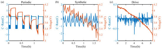
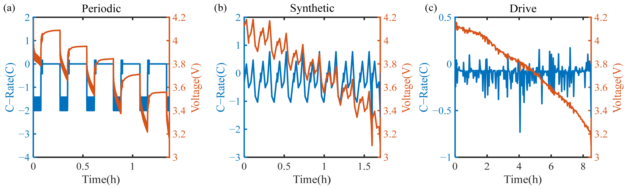
The dataset includes three categories of operating conditions, namely Periodic, Synthetic, and Drive, covering a wide range of dynamic load complexities from controlled laboratory protocols to real-world vehicle operation. The Periodic protocols were designed to emulate dynamic discharge and regenerative braking behaviors commonly encountered in electric vehicles. The Synthetic protocols were generated from real urban driving data and represent typical highway driving, urban driving, and mixed driving scenarios. The Drive protocols were directly derived from actual electric vehicle driving data collected in two different cities.

(2)

Significant variations in temporal characteristics across load profiles

The dynamic cycling protocols differ substantially in terms of average current rate, excitation structure, and excitation duration, providing a rich data foundation for investigating the timescale dependency of SOH-related information. Short-duration dynamic excitations tend to emphasize fast-response characteristics such as polarization dynamics and internal resistance variations, whereas longer-duration load processes are more likely to reveal slow degradation behaviors associated with capacity fade. Consequently, the voltage responses under different operating conditions simultaneously contain both fast-varying and slow-varying degradation information, creating favorable conditions for analyzing the influence of observation timescale selection on SOH estimation performance.

In total, the dataset contains 69 battery samples distributed across the three operating conditions. As summarized in Table 1, the Periodic, Synthetic, and Drive conditions include 30, 31, and 8 cells, respectively. Cycling tests were conducted under different average C-rates, including C/16, C/10, C/5, and C/2. The Periodic protocols consist of discharge pulses, short charging pulses that emulate regenerative braking, and rest periods. By varying charge–discharge ratios, excitation frequencies, current amplitudes, and multi-frequency signal combinations, five representative periodic protocols (A–E) were constructed. The Synthetic protocols include six representative driving scenarios, namely highway short-trip (1a), highway long-trip (1b), urban driving (2a, 2b, and 2c), and mixed highway-urban driving (3). The Drive protocols were generated by converting real vehicle speed trajectories into corresponding battery current load profiles. Due to current limitations of the experimental equipment, some high-rate dynamic protocols were not tested under all C-rate conditions.

Table 1. Summary of battery samples under different dynamic operating conditions from Ref. [35].

Condition Type	Condition Description	Protocol Average C-Rate
		C/16	C/10	C/5	C/2
Periodic	A: Reference		25, 26	33, 34	41, 42
	B: Charge–Discharge Ratio		27, 28	35, 36	43, 44
	C: High Current Amplitude		29, 30	37, 38	45, 46
	D: Frequency		31, 32	39, 40	47, 48
	E: Superposition		49, 50	51, 52	53, 54
Synthetic	1a: Highway (short trips)	57, 58	59, 60	61, 62
	1b: Highway (long trips)	63, 64	71, 72
	2a: Urban (City 1)		65, 66	67, 68	69, 70
	2b: Urban (City 2)		73, 74	75, 76	77, 78
	2c: Urban (City 1 + 2)		81, 82	84	85, 86
	3: Highway + Urban		79, 80	87, 88
Drive	City 1: Full Day	89, 90	91, 92
	City 2: Full Day	93, 94	95, 96

Figure 1 presents representative current and voltage profiles under the three dynamic operating conditions. Compared with conventional constant-current discharge tests, these dynamic protocols more realistically capture the load variations experienced by traction batteries during practical vehicle operation, thereby providing a solid data foundation for subsequent SOH estimation and degradation feature analysis.

Figure 1. Representative voltage and current profiles under different dynamic operating conditions: (a) Periodic; (b) Synthetic; and (c) Drive.

3. Methodology

3.1. Overview Framework for SOH Estimation

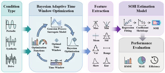
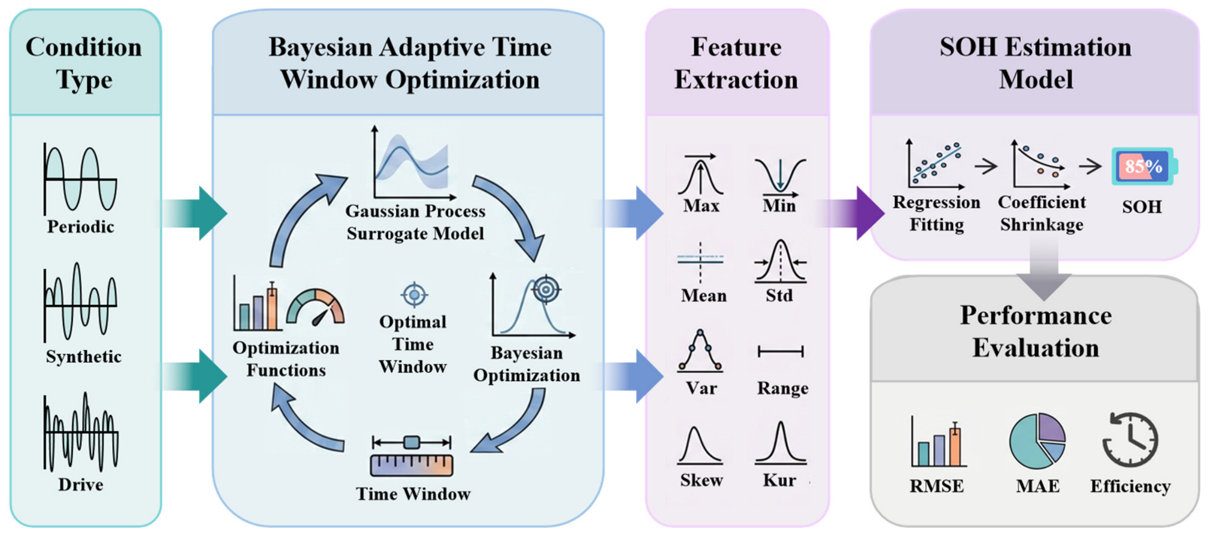
The overall framework for SOH estimation is illustrated in Figure 2, which consists of three major components: (1) a Bayesian optimization-based adaptive time window search module; (2) a timescale-aware statistical feature extraction module; and (3) a lightweight regression-based SOH estimation module.

Figure 2. Bayesian Adaptive Time Window Optimization framework for feature extraction in SOH estimation of lithium-ion batteries.

The proposed BATWO framework is specifically designed for feature extraction under dynamic operating conditions. The key idea is to treat the predefined time window length as a learnable parameter and enable adaptive time window selection.

Employ Bayesian optimization to identify the optimal time window under different operating conditions. Unlike conventional fixed time window approaches, the BATWO framework explicitly models the nonlinear relationship between observation timescale and SOH, enabling data-driven adaptation of temporal structures. The framework automatically identifies the most informative timescale for degradation observation, thereby improving the extraction of degradation-sensitive features from dynamic voltage responses. As a result, SOH-related information can be captured more effectively under varying operating conditions, providing a solid feature foundation for accurate, interpretable, and computationally efficient SOH estimation.

3.2. Bayesian Adaptive Time Window Optimization

3.2.1. Problem Formulation

Under dynamic operating conditions, the battery discharge voltage sequence exhibits pronounced non-stationary characteristics and can be represented as:

$$V={\left\{v\left(t\right)\right\}}_{t=1}^T$$

(1)

where v(t) denotes the voltage observation at time t, and T is the length of the voltage sequence.

Given a time window length w, a local temporal segment can be defined as:

$$V_w={\left\{v\left(t\right)\right\}}_{t=t_0}^{t_0+w}$$

(2)

Based on the extracted local sequence, the SOH estimation process can be formulated as:

$$\stackrel{\wedge }{y}=f\left(\mathsf{\Psi }\left(V_w\right)\right)$$

(3)

where $\mathsf{\Psi }\left(•\right)$ represents the feature extraction operator, and $f\left(•\right)$ denotes the regression mapping function from the feature space to the SOH space.

In this study, the time window optimization problem is formulated as:

$$w^{*}=\underset{w\in \left[w_{\min },w_{\max }\right]}{\arg \min }\mathsf{\Gamma }\left(w\right)$$

(4)

where $\mathsf{\Gamma }\left(w\right)$ denotes the objective function associated with the time window w.

3.2.2. Design of Multi-Objective Optimization Functions

To simultaneously account for prediction accuracy and degradation representation consistency, a multi-objective optimization function is defined as:

$$\mathsf{\Gamma }\left(w\right)={\displaystyle \frac{\mathrm{RMSE}\left(w\right)+\mathrm{MAE}\left(w\right)}{\overline{\mathrm{SOH}}}}-\lambda \cdot C\left(w\right)$$

(5)

In the above formulation, RMSE(w) and MAE(w) denote the Root Mean Square Error (RMSE) and Mean Absolute Error (MAE), respectively, obtained by training the SOH estimation model using features extracted from the time window w. $\overline{\mathrm{SOH}}$ represents the normalized mean SOH value used to reduce the influence of scale differences among operating conditions. C(w) denotes the average correlation between the extracted features and SOH, reflecting the degradation sensitivity of the selected observation timescale. The parameter λ is a weighting coefficient that balances prediction accuracy and degradation-related feature relevance in the objective function. In this study, λ is empirically set to 0.5 to achieve a balanced contribution between the two terms. Its robustness is further verified through sensitivity analysis with λ values ranging from 0 to 1, which demonstrates negligible influence on the final optimization results.

By incorporating both prediction-error metrics and feature-SOH correlation information, the proposed objective function enables the optimization process to identify observation timescales that not only achieve high estimation accuracy but also provide stronger degradation observability, thereby improving the interpretability and robustness of the extracted HIs.

3.2.3. Bayesian Optimization Strategy

Due to the complex nonlinear relationship between the time window length and the objective function, as well as the high computational cost associated with each objective-function evaluation, which involves feature extraction, model training, and performance validation, Bayesian Optimization is adopted to determine the optimal time window length.

In this study, the observation time window is optimized as an integer variable with a search resolution of 1 s. The search range is set from 500 s to 60% of the discharge duration corresponding to the average C-rate under each operating condition. Bayesian Optimization is implemented using the Gaussian Process surrogate model with the Matérn kernel and the Expected Improvement (EI) acquisition function. The maximum number of objective-function evaluations is set to 15, and a fixed random seed of 42 is used to ensure reproducibility. The initialization of sampling points follows the default strategy of the Scikit-Optimize library, where 10 initial points are randomly sampled before constructing the Gaussian Process surrogate model.

Bayesian optimization is a global optimization framework designed for black-box optimization problems. Its fundamental idea is to approximate the objective function using a surrogate model and to guide the selection of the next sampling location through an acquisition function, thereby identifying the global optimum with a limited number of objective-function evaluations.

In this study, a Gaussian Process (GP) is employed as the surrogate model and is defined as:

$$\mathsf{\Gamma }\left(w\right)\sim GP\left(\mu \left(w\right),k\left(w,w^{\prime }\right)\right)$$

(6)

where μ(w) denotes the mean function and k(•) represents the Matérn covariance kernel adopted in this study.

The GP constructs a probabilistic surrogate model using previously evaluated time window lengths and their corresponding objective-function values, thereby approximating the mapping between the time window length and the optimization objective. Unlike conventional regression models, the GP not only predicts the objective value but also quantifies the uncertainty associated with the prediction. Consequently, compared with grid-search methods that require exhaustive evaluation of all candidate time windows, Bayesian optimization can approach the global optimum with significantly fewer evaluations.

Let the set of evaluated time window lengths be defined as:

$$D_t={\left\{\left(w_i,\mathsf{\Gamma }\left(w_i\right)\right)\right\}}_{i=1}^t$$

(7)

After the t-th iteration, the GP provides the posterior predictive distribution for a candidate time window w:

$$\left.\mathsf{\Gamma }\left(w\right)\right|D_t\sim N\left({\mu }_t\left(w\right),{{\sigma }_t}^2\left(w\right)\right)$$

(8)

where ${\mu }_t\left(w\right)$ and ${{\sigma }_t}^2\left(w\right)$ denote the posterior predictive mean and the posterior predictive variance, respectively. The predictive mean reflects the expected optimization performance of the candidate time window, whereas the predictive standard deviation characterizes the uncertainty of the surrogate model in that region. Regions with limited observations generally exhibit higher uncertainty, indicating greater potential value for further exploration.

To balance exploitation and exploration during the optimization process, the EI criterion is adopted as the acquisition function. The acquisition function evaluates the sampling value of each candidate time window based on the current GP predictions and determines the next location for objective-function evaluation.

Since the objective function considered in this study is formulated as a minimization problem, let the best objective value observed so far be:

$${\mathsf{\Gamma }}_{\min }=\underset{i=1,2,\mathrm{\dots },t}{\min }\mathsf{\Gamma }\left(w_i\right)$$

(9)

The improvement associated with a candidate window w is defined as:

$$I\left(w\right)=\max \left({\mathsf{\Gamma }}_{\min }-\mathsf{\Gamma }\left(w\right),0\right)$$

(10)

Because the true objective value f(w) is unknown, its expectation under the GP predictive distribution is calculated, resulting in the Expected Improvement function:

$$\mathrm{{\rm E}}\mathrm{{\rm I}}(w)=\mathit{{\rm E}}\left[I\left(w\right)\right]$$

(11)

Based on the GP posterior distribution, the EI criterion can be expressed analytically as:

$$\mathrm{{\rm E}}\mathrm{{\rm I}}(w)=\left({\mathsf{\Gamma }}_{\min }-{\mu }_t\left(w\right)\right)\mathsf{\Phi }\left(Z\right)+{\sigma }_t\left(w\right)\phi \left(Z\right)$$

(12)

where $Z={\displaystyle \frac{{\mathsf{\Gamma }}_{\min }-{\mu }_t\left(w\right)}{{\sigma }_t\left(w\right)}}$ is the standardized residual variable, $\mathsf{\Phi }\left(\cdot \right)$ and $\phi \left(\cdot \right)$ denote the cumulative distribution function (CDF) and probability density function (PDF) of the standard normal distribution, respectively.

The EI criterion simultaneously considers the predicted objective value and the associated uncertainty. A lower predicted objective value increases the first term of the EI expression, encouraging exploitation of promising regions. In contrast, a larger predictive uncertainty increases the second term, promoting exploration of insufficiently sampled regions. Therefore, EI achieves an effective balance between exploitation and exploration and helps prevent premature convergence to local optima.

At each iteration, the next candidate time window is selected by maximizing the acquisition function:

$$w_{t+1}=\arg {\max }_{w}EI\left(w\right)$$

(13)

In other words, the time window with the greatest expected improvement is selected for objective-function evaluation. It should be emphasized that Bayesian optimization does not directly optimize the objective function itself. Instead, it determines the next sampling location by maximizing the EI criterion. For minimization problems, a larger EI value indicates a greater probability of achieving further improvement over the current best solution. Therefore, maximizing EI is consistent with the ultimate objective of minimizing the target function.

After obtaining the objective value of the newly selected time window, the corresponding observation is incorporated into the dataset, and the GP posterior distribution is updated accordingly. As the optimization proceeds, the surrogate model progressively learns the nonlinear relationship between the time window length and the objective function, continuously refining its representation of the search space. During this process, the predictive mean gradually approaches the true objective-function landscape, while the predictive uncertainty decreases around promising regions, enabling computational resources to be focused on potentially optimal solutions.

Through iterative updates of the posterior distribution and acquisition function, Bayesian optimization progressively approximates the relationship between the time window length and prediction performance, ultimately identifying the optimal time window length w*. Compared with conventional grid-search approaches that require exhaustive evaluation of all candidate time windows, Bayesian optimization effectively exploits historical search information to guide subsequent sampling decisions. As a result, it substantially reduces computational cost while achieving superior timescale selection, thereby providing an optimal observation time window for subsequent statistical feature extraction and SOH estimation.

3.3. Feature Extraction Under the Optimized Time Window

After obtaining the optimal time window w*, SOH-related features are extracted from the corresponding voltage sequence. The voltage segment within the optimized observation time window can be represented as:

$$V=\left\{v_1,v_2,\mathrm{\dots },v_n\right\}$$

(14)

Based on this local dynamic voltage sequence, eight HIs are extracted and defined as follows:

$$F_{\max }=\max \left(v_i\right)$$

(15)

$$F_{\min }=\min \left(v_i\right)$$

(16)

$$F_{\mathrm{mean}}={\displaystyle \frac{1}{n}}{\displaystyle \sum _{i=1}^n{v}_i}$$

(17)

$$F_{\mathrm{std}}=\sqrt{{\displaystyle \frac{1}{n}}{\displaystyle \sum _{i=1}^n{\left(v_i-\overline{v}\right)}^2}}$$

(18)

$$F_{\mathrm{var}}={\displaystyle \frac{1}{n}}{\displaystyle \sum _{i=1}^n{\left(v_i-\overline{v}\right)}^2}$$

(19)

$$F_{\mathrm{range}}=F_{\max }-F_{\min }$$

(20)

$$F_{\mathrm{skew}}={\displaystyle \frac{1}{n}}{\displaystyle \sum _{i=1}^n{\left(\frac{v_i-\overline{v}}{{\sigma }_v}\right)}^3}$$

(21)

$$F_{\mathrm{kur}}={\displaystyle \frac{1}{n}}{\displaystyle \sum _{i=1}^n{\left(\frac{v_i-\overline{v}}{{\sigma }_v}\right)}^4}$$

(22)

where $\overline{v}=F_{\mathrm{mean}}$ and ${\sigma }_v=F_{\mathrm{std}}$ denote the mean and standard deviation of the voltage sequence within the observation time window, respectively.

Among the extracted features, F_max, F_min and F_mean characterize the overall voltage level within the local observation time window. F_std, F_var and F_range quantify the magnitude of voltage fluctuations under dynamic load conditions. Meanwhile, F_skew and F_kur describe the shape characteristics of the voltage distribution, including its asymmetry and peakedness. These HIs provide complementary descriptions of battery voltage responses from multiple perspectives and capture degradation-related information embedded in dynamic operating conditions.

3.4. Feature Selection Based on Correlation Analysis

Since different statistical features exhibit varying levels of sensitivity to SOH degradation, a correlation-based feature selection strategy is further introduced to improve feature quality and reduce the influence of redundant information. Pearson correlation is adopted to quantify the relationship between extracted statistical features and battery capacity, since the extracted features are expected to reflect degradation-related variations in SOH and the subsequent SOH estimation model is also based on a linear regression framework.

For each statistical feature F_i, the Pearson correlation coefficient between each feature and battery capacity is calculated as:

$${\rho }_i=corr\left(F_i,\mathrm{SOH}\right)$$

(23)

Based on the calculated correlation coefficients, the selected feature subset is defined as:

$$\mathrm{{\rm P}}=\left\{\left.F_i\right|\left|{\rho }_i\right|\ge 0.7\right\}$$

(24)

In this study, the Pearson correlation threshold is set to 0.7, as an absolute correlation coefficient above 0.7 is generally considered a strong linear correlation and provides a reasonable criterion for retaining degradation-sensitive features while reducing redundant information. Moreover, the robustness of this setting is verified through sensitivity analysis with thresholds ranging from 0.5 to 0.9, where only minor variations in selected feature subsets are observed, and the SOH estimation performance remains nearly unchanged. In cases where no feature satisfies the selection criterion under a specific observation time window, all extracted features are retained to avoid potential information loss.

To quantify the overall degradation relevance of the selected features under a given observation timescale, a window-level average correlation metric is further defined as:

$$C\left(w\right)={\displaystyle \frac{1}{\left|\mathrm{{\rm P}}\right|}}\left\{{\displaystyle \sum _{F_i\in \mathrm{{\rm P}}}\left|\left.{\rho }_i\right|\right.}\right\}$$

(25)

The metric characterizes the structural consistency between the extracted statistical features and battery degradation at a given timescale. Meanwhile, this metric is fed back to the Bayesian optimization procedure.

3.5. Lightweight SOH Estimation Model Construction

After completing the time window optimization, statistical feature extraction, and correlation-based feature selection within the proposed BATWO framework, a lightweight regression model is employed for SOH estimation. Considering the trade-off between practical deployment requirements and model interpretability, ElasticNet Regression is selected as the primary prediction model.

ElasticNet combines the advantages of both L1-norm and L2-norm regularization. Its objective function can be formulated as:

$$\underset{\beta }{\min }{‖\mathit{y}-\mathit{{\rm X}}\beta ‖}_2^2+{\alpha }_1{‖\beta ‖}_1+{\alpha }_2{‖\beta ‖}_2^2$$

(26)

where X denotes the statistical feature matrix extracted and selected by the BATWO framework, y represents the corresponding ground-truth SOH values, β is the regression coefficient vector, and α₁ and α₂ control the strengths of the L1 and L2 regularization terms, respectively.

The L1 regularization term promotes feature sparsity, thereby improving robustness against redundant or less informative features. Meanwhile, the L2 regularization term enhances model stability and generalization capability by mitigating parameter variance. Therefore, potentially redundant statistical features, such as standard deviation and variance, can be effectively regulated by ElasticNet during model fitting. As a result, ElasticNet is particularly suitable for the low-dimensional statistical feature space constructed in this study, offering a favorable balance between prediction accuracy and model interpretability.

4. Results and Discussion

To comprehensively evaluate the SOH estimation performance of the proposed BATWO framework under dynamic operating conditions, experiments were conducted across different combinations of condition types and protocol average C-rate levels. For each battery cell, the first 80% of cycling samples were used for training, while the remaining 20% were reserved for testing. The partitioning was performed chronologically to ensure that only historical degradation information was available during model development, whereas future cycling data were used exclusively for final evaluation. Although samples from the same cell are included in both subsets, the two subsets correspond to different chronological degradation stages. The training process only utilizes earlier-cycle information, while later-cycle degradation behaviors are completely reserved for testing, thereby preventing the model from accessing future degradation information. All optimization procedures, including observation-window determination, feature selection, feature normalization, and ElasticNet hyperparameter tuning, were performed using only the training samples. Specifically, BATWO determines one optimal observation window using the training data from all cells under the same combination of condition types and protocol average C-rate levels, and this window is then uniformly applied to the corresponding test samples. No testing samples were involved in any stage of model selection or optimization. Cross-validation was conducted only within the training dataset to determine optimal configurations, while the testing dataset was exclusively used for the final performance evaluation. After the optimization process, all parameters were fixed, and the test dataset was used solely for evaluating the final SOH estimation performance.

To quantitatively assess SOH estimation performance, two widely adopted evaluation metrics, namely the RMSE and the MAE, were employed. These metrics are defined as follows:

$$RMSE=\sqrt{{\displaystyle \frac{1}{N}}{\displaystyle \sum _{i=1}^N{\left(y_i-\stackrel{\wedge }{y_i}\right)}^2}}$$

(27)

$$MAE={\displaystyle \frac{1}{N}}{\displaystyle \sum _{i=1}^N\left|\left.y_i-\stackrel{\wedge }{y_i}\right|\right.}$$

(28)

where N denotes the number of testing samples, y_i represents the true SOH value of the i-th sample and ŷ_i denotes the corresponding predicted SOH value.

4.1. Bayesian Adaptive Time Window Optimization Results

To evaluate the timescale learning capability of the proposed BATWO framework under dynamic operating conditions, the optimal time windows and corresponding SOH estimation results for different operating conditions are first analyzed, as summarized in Table 2.

Table 2. Results for adaptive time window optimization with BATWO framework under different dynamic operating conditions.

Condition Type	Average C-Rate	Best Time Window (s)	RMSE (%)	MAE (%)	Selected Features	Selected Correlations
Periodic	C/10	500	3.74	1.81	Fmax	0.95
	C/5	500	1.91	1.50	Fmax	0.97
	C/2	3543	2.14	1.79	Fmax	0.98
Synthetic	C/16	6748	2.18	1.72	Fmax	0.97
	C/10	500	3.14	2.25	Fmin, Frange, Fvar	0.89, −0.87, −0.72
	C/5	5092	1.55	0.90	Fmax, Fmin, Fmean, Frange, Fstd, Fvar, Fskew, Fkur	0.25, 0.25, 0.41, −0.24, −0.24, −0.24, −0.54, 0.31
	C/2	3507	1.69	1.30	Fmin, Fmean, Frange, Fstd, Fvar	0.88, 0.86, −0.98, −0.98, −0.97
Drive	C/16	27,630	0.79	0.61	Fmax	0.98
	C/10	16,951	1.48	1.21	Fmax	0.98

As shown in Table 2, the optimal time window lengths vary substantially across different dynamic operating conditions, ranging from 500 s to 27,630 s. The Periodic and Synthetic conditions generally require relatively short windows, whereas the Drive conditions favor longer timescales. This result indicates that SOH-related degradation information exhibits strong timescale dependency for different operating profiles. Notably, even operating conditions with the same average C-rate can correspond to markedly different optimal time windows. For example, the Periodic C/10, Synthetic C/10, and Drive C/10 conditions all share the same average discharge C-rate, yet their optimal time windows differ considerably. This observation suggests that the optimal observation timescale is determined not only by load intensity but also by the characteristics of the operating profile.

In terms of estimation performance, BATWO achieves high prediction accuracy across most operating conditions. For the Periodic conditions, the RMSE ranges from 1.91% to 3.74%, while the Synthetic conditions yield RMSE values between 1.55% and 3.14%. The lowest prediction errors are observed under the Drive conditions, where the RMSE values for Drive C/16 and Drive C/10 are only 0.79% and 1.48%, respectively. It is noteworthy that the C/10 cases consistently exhibit relatively larger prediction errors within both the Periodic and Synthetic condition groups, with RMSE values reaching 3.74% and 3.14%, respectively. In contrast, the Drive conditions achieve the highest estimation accuracy despite their significantly longer time windows. The Drive condition includes intermittent intervals between dynamic load variations, making the effective excitation duration shorter than the total observation window. These results demonstrate that the proposed BATWO framework can effectively identify operating-condition-specific observation timescales and achieve consistently accurate SOH estimation under diverse dynamic operating conditions.

The feature-selection results further reveal the distribution characteristics of degradation information under different operating conditions. For both the Periodic and Drive conditions, F_max is consistently selected as the optimal feature and maintains a strong correlation with SOH (greater than 0.95 in all cases), indicating that the maximum voltage statistic effectively captures the capacity degradation process under these load profiles. In contrast, the more complex Synthetic conditions require multiple statistical features to jointly characterize SOH, including F_min, F_mean, F_range, F_std and F_var. This observation suggests that degradation information in these conditions is reflected not only in changes in voltage level but also in voltage fluctuation characteristics.

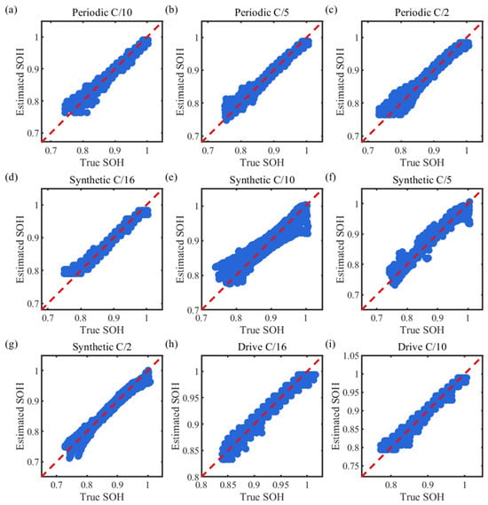
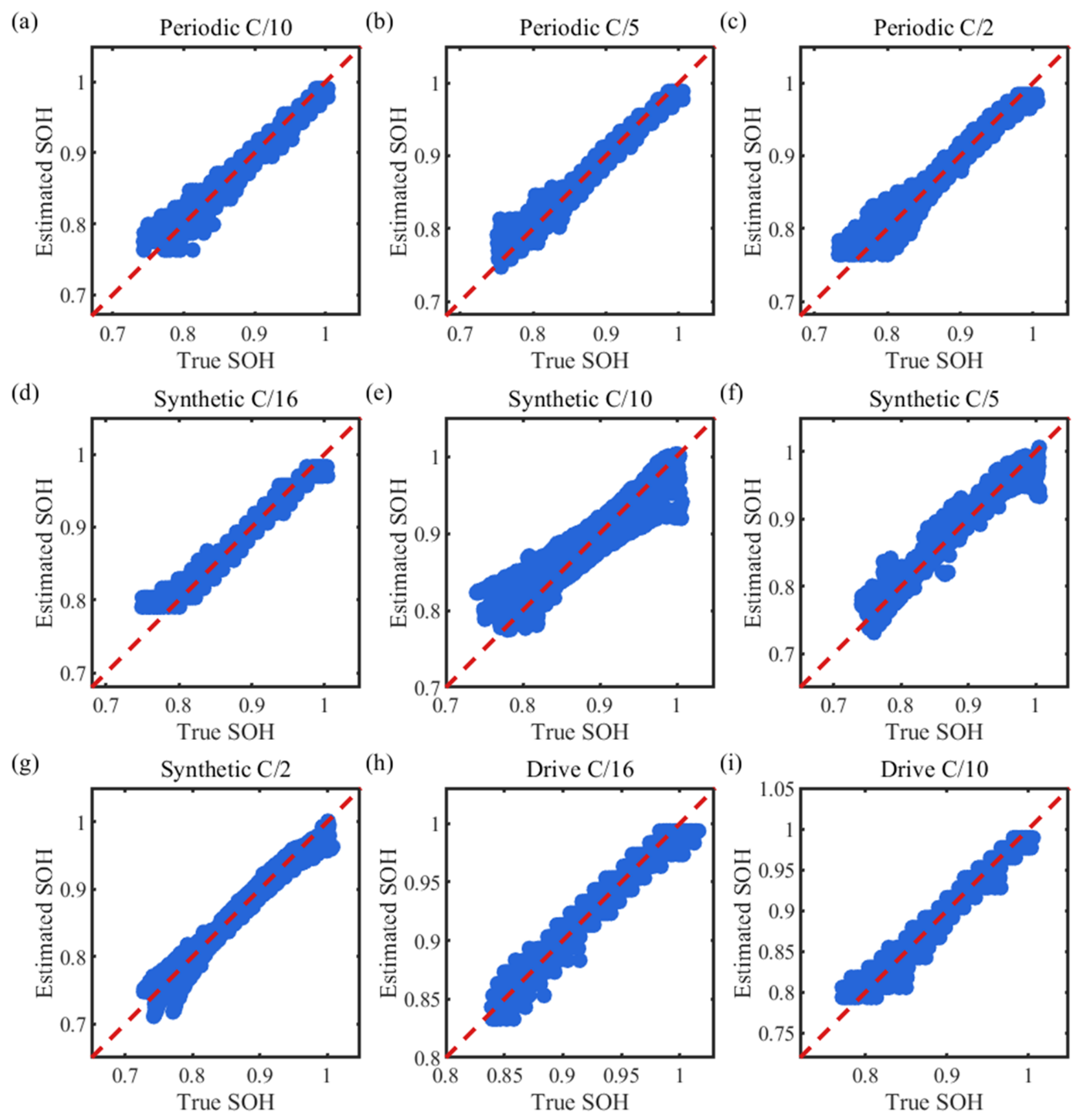
Figure 3 presents the scatter plots between the estimated and measured capacities for all operating conditions. It can be observed that the predicted capacities exhibit strong agreement with the corresponding ground-truth values, indicating that the statistical features extracted under the optimized observation timescales effectively capture battery degradation behavior.

Figure 3. Comparison of estimated and measured battery SOH under different dynamic operating conditions: (a–c) Periodic, (d–g) Synthetic, and (h,i) Drive.

These results suggest that the proposed BATWO framework is capable of automatically learning the optimal degradation observation timescale for different dynamic operating conditions and constructing the corresponding statistical degradation structures. By jointly optimizing observation timescale and feature representation, BATWO improves degradation observability and supports accurate SOH estimation across a wide range of dynamic operating scenarios.

4.2. Comparative Analysis with the Deep Learning Baselines

To further validate the effectiveness of the statistical degradation features constructed within the proposed BATWO framework, a comparative study is conducted using two representative deep learning models as benchmarks, namely LSTM and Transformer. For a fair comparison, the observation window and model-specific hyperparameters of each method are independently optimized using Bayesian optimization, with the validation RMSE adopted as the optimization objective. Specifically, the BATWO-based approach first extracts HIs from the optimized time window and employs an ElasticNet regression model for SOH prediction. In contrast, both LSTM and Transformer directly utilize the raw voltage time series within the same window and are trained in an end-to-end manner. During optimization, the hidden units and learning rate of LSTM, as well as the attention heads, key dimension, feed-forward dimension, dropout rate, and learning rate of Transformer, are tuned separately to ensure a fair and unbiased comparison among different modeling strategies. The optimized configurations obtained for each operating condition were directly adopted for the final evaluation.

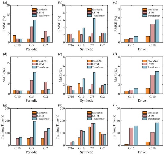
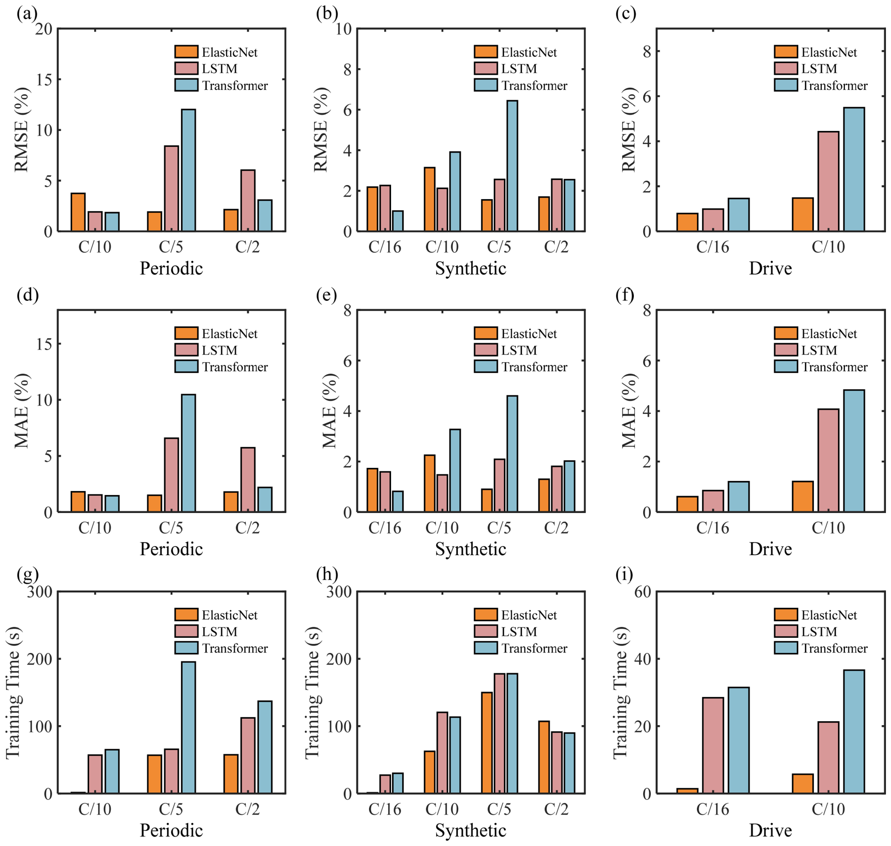
In addition to prediction accuracy, training time is also introduced as an evaluation metric to assess computational efficiency and practical deployment potential. Figure 4 presents the RMSE, MAE, and training time results of the three methods under different dynamic operating conditions. Overall, the proposed BATWO framework consistently achieves the best prediction performance across all operating scenarios.

Figure 4. Comparison of SOH estimation accuracy and training time among ElasticNet, LSTM, and Transformer under different dynamic operating conditions: (a–c) RMSE, (d–f) MAE, and (g–i) training time.

Under the Periodic conditions, ElasticNet achieves the best prediction accuracy across all C-rate settings. As shown in Figure 4a and Figure 4d, the RMSE under the Periodic C/5 condition is reduced by approximately 77.3% and 84.1% compared with LSTM and Transformer, respectively. Under the Periodic C/2 condition, BATWO further reduces the RMSE to 2.14%, whereas LSTM and Transformer obtain 6.04% and 3.08%, respectively. For the Synthetic conditions, the three methods exhibit relatively comparable performance. ElasticNet achieves the lowest estimation errors under the C/5 and C/2 conditions, while Transformer performs best under C/16. Under the Drive conditions, BATWO consistently provides the most accurate SOH estimation. In particular, under the Drive C/16 condition, the RMSE and MAE are only 0.79% and 0.61%, respectively, and the RMSE is reduced by approximately 20.2% and 45.9% compared with LSTM and Transformer. Similar improvements are also observed under the Drive C/10 condition. Since the Drive dataset is collected from real vehicle operating profiles, these results indicate that the proposed statistical degradation representation generalizes well to practical operating scenarios.

In addition to accuracy improvements, BATWO also demonstrates significant advantages in computational efficiency. As shown in Figure 4g–i, the ElasticNet model typically requires only a few seconds for training across most operating conditions, whereas LSTM and Transformer often require tens to hundreds of seconds. It is worth noting that due to the large variation in training time scales, the bars corresponding to ElasticNet in these figures appear close to the horizontal axis and may visually underestimate its advantage. For instance, under the Periodic C/10, Synthetic C/16, and Drive C/16 conditions, the training times of ElasticNet are only 1.39 s, 1.03 s, and 1.41 s, respectively, while those of LSTM and Transformer all exceed 25 s, representing a reduction in training time of more than 95%.

These results demonstrate that, compared with direct deep learning on raw time-series data, the proposed BATWO-based statistical degradation representation provides more informative SOH-related representations while significantly reducing model complexity and training cost. Overall, the experimental results further validate the effectiveness of the proposed framework in achieving accurate, lightweight, and computationally efficient SOH estimation under dynamic operating conditions.

4.3. Comparative Analysis with Other Machine Learning Models

To further evaluate the effectiveness of different machine learning models in exploiting the features extracted by BATWO, three representative regression models, i.e., ElasticNet, SVR, and XGBoost, are employed for SOH estimation under the same time window optimization and statistical feature construction pipeline.

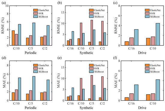
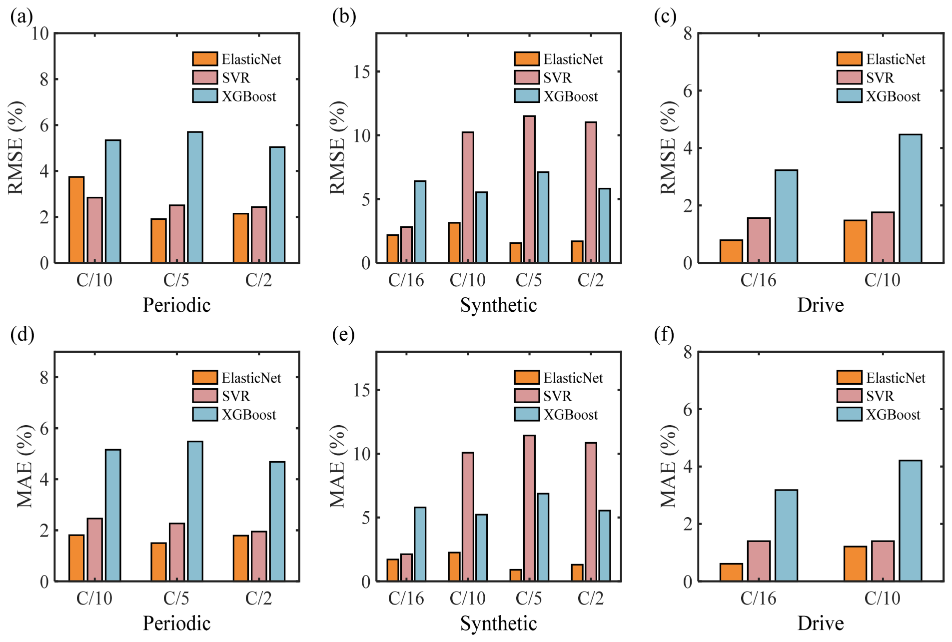
Overall, ElasticNet achieves the best prediction performance across most operating conditions. For the Periodic conditions, both ElasticNet and SVR can provide relatively accurate SOH estimation. As shown in Figure 5a and Figure 5d, under the Periodic C/5 condition, ElasticNet achieves an RMSE and MAE of 1.91% and 1.50%, respectively, outperforming SVR, which yields 2.51% and 2.27%. In contrast, XGBoost shows relatively large prediction errors under all Periodic conditions, with RMSE values consistently exceeding 5%. For the Synthetic conditions, the performance gap among different models becomes more pronounced. ElasticNet consistently achieves the best results across all C-rate settings. As illustrated in Figure 5b and Figure 5e, the RMSE values for the Synthetic C/5 and C/2 conditions are only 1.55% and 1.69%, respectively. In comparison, SVR suffers from significant performance degradation, with RMSE generally exceeding 10%, while XGBoost performs better than SVR but still remains clearly inferior to ElasticNet. Under the Drive conditions, ElasticNet again demonstrates the most accurate performance. As shown in Figure 5c and Figure 5f, the RMSE values under Drive C/16 and C/10 are only 0.79% and 1.48%, respectively, both lower than those of SVR and XGBoost. In particular, under the Drive C/16 condition, ElasticNet achieves approximately 49% and 76% error reduction compared with SVR and XGBoost, respectively, further confirming its effectiveness on real-world driving data.

Figure 5. RMSE and MAE comparison of SOH estimation performance obtained by different machine learning models under dynamic operating conditions: (a,d) Periodic, (b,e) Synthetic, and (c,f) Drive.

Although SVR and XGBoost possess stronger nonlinear modeling capabilities, ElasticNet is able to more effectively exploit the degradation information embedded in the low-dimensional statistical feature space constructed by BATWO, thereby achieving higher prediction accuracy and more stable generalization performance. These results indicate that the optimized time window selection and feature screening process has already yielded a highly informative degradation representation of SOH evolution, making complex nonlinear models unnecessary. Consequently, the combination of BATWO and ElasticNet achieves a favorable balance among prediction accuracy, model complexity, and practical deployability.

4.4. Comparison with Fixed Time Window Strategies

To further validate the necessity of adaptive time window optimization for SOH estimation, the proposed BATWO framework is compared with conventional fixed time window strategies. In the fixed time window approach, feature extraction is performed using predefined window lengths of 1200 s, 2400 s, and 3600 s from the beginning of the discharge process for all operating conditions. The best-performing and worst-performing fixed time window results are selected as baselines for comparison.

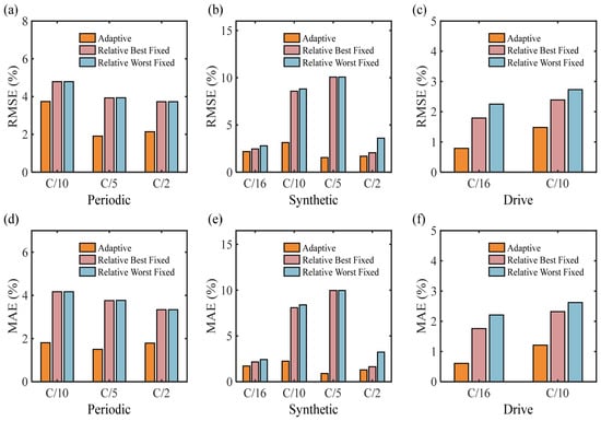
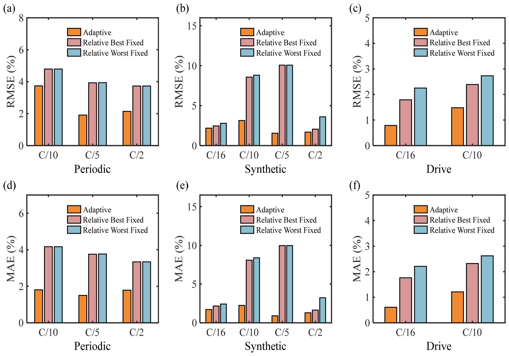
Figure 6 presents a comparison of RMSE and MAE between the adaptive time window method and fixed time window strategies under different dynamic operating conditions. Overall, the fixed time window approach exhibits significant instability across different scenarios, with its performance being highly sensitive to the choice of window length. In particular, under more complex operating conditions such as Synthetic C/10, the prediction error increases substantially when inappropriate window lengths are used. In contrast, the proposed adaptive time window method consistently achieves more stable and superior performance across all operating conditions.

Figure 6. RMSE and MAE comparison of adaptive and fixed time window strategies under different dynamic operating conditions: (a,d) Periodic, (b,e) Synthetic, and (c,f) Drive.

Table 3 further summarizes the overall performance comparison. Compared with the best fixed time window strategy, the adaptive method achieves average improvements of 2.35 and 2.68 percentage points in RMSE and MAE, respectively. When compared with the worst fixed time window strategy, the improvements are further increased to 2.68 and 3.00 percentage points. In terms of extreme cases, the maximum improvements reach 8.52 and 9.07 percentage points in RMSE and MAE, respectively, indicating that poorly selected time window lengths can severely degrade feature representation capability in fixed time window methods, whereas the proposed BATWO framework with adaptive time window optimization effectively mitigates this issue. Notably, no performance degradation is observed across all test scenarios, indicating the robustness of the proposed approach.

Table 3. Overall performance comparison between adaptive and fixed time window strategies.

Comparison Metric	RMSE (%)	MAE (%)
Average improvement over the best fixed time window	+2.35	+2.68
Average improvement over the worst fixed time window	+2.68	+3.00
Maximum improvement over the fixed time window	+8.52	+9.07
Number of cases outperforming the best fixed time window	9/9	9/9

In summary, the fixed time window strategy suffers from inherent limitations due to its lack of adaptability to varying operating conditions and timescale differences. In contrast, the BATWO framework dynamically adjusts the feature extraction timescale according to different operating scenarios through an adaptive time window searching module, thereby achieving more stable and superior SOH estimation performance across diverse dynamic discharge conditions.

4.5. Comparison of Different Time Window Optimization Strategies

To further evaluate the optimization efficiency of BATWO, Grid Search and Random Search are introduced as comparison methods under the same feature extraction procedure, SOH estimation model, candidate window range, and optimization objective. Grid Search exhaustively evaluates all candidate windows within the predefined search space, ensuring comprehensive exploration but requiring a large number of computationally expensive evaluations. Random Search reduces the search burden by randomly sampling candidate windows; however, it does not exploit the information obtained from previous evaluations and may result in inefficient exploration. In contrast, BATWO employs Bayesian Optimization to iteratively update a surrogate model based on historical evaluation results and select informative candidate windows through an acquisition function. By learning the relationship between the observation window length and SOH estimation performance, BATWO can focus subsequent evaluations on promising regions of the search space and efficiently identify suitable degradation-sensitive timescales.

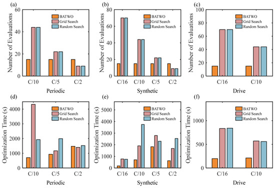
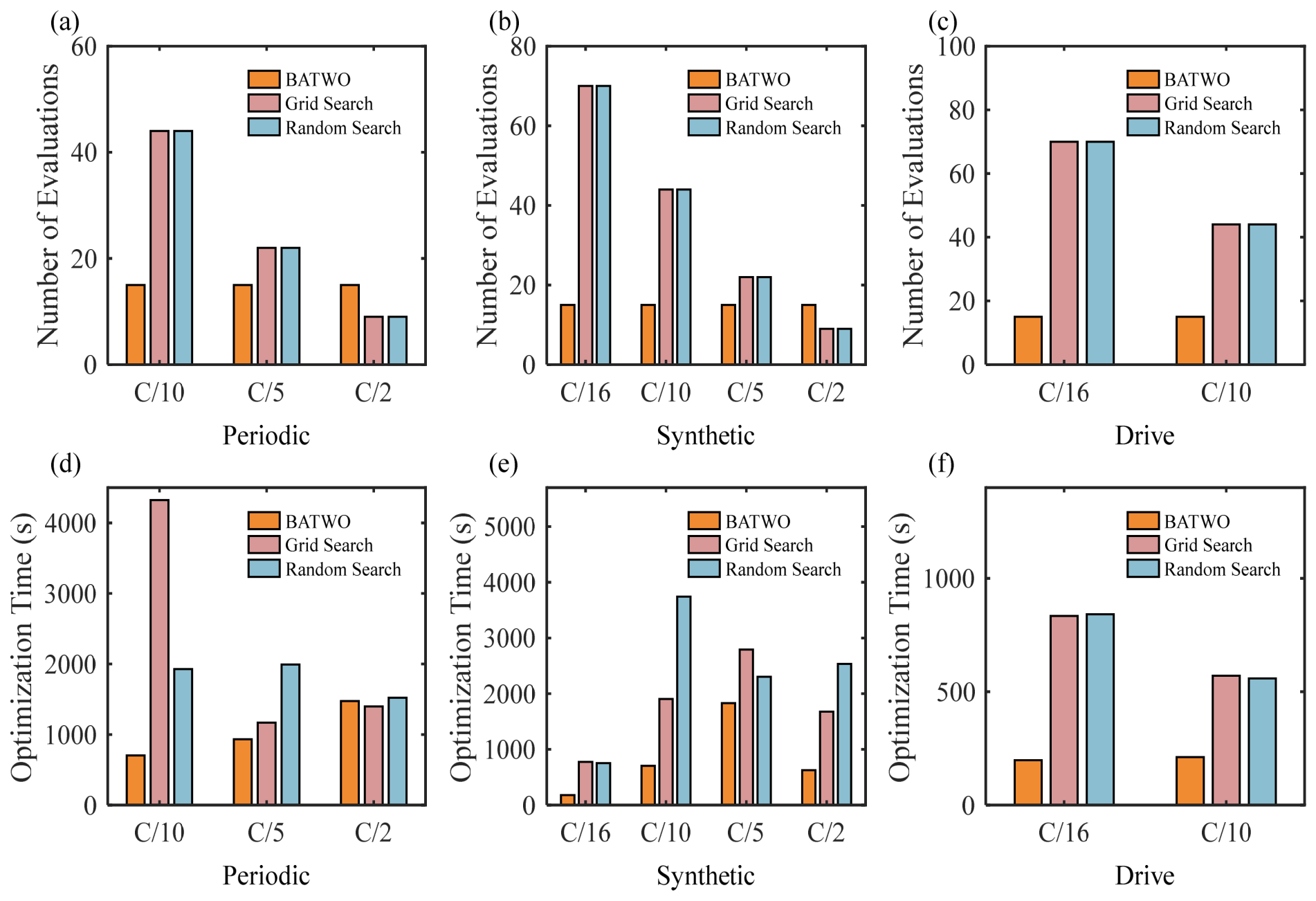
Figure 7 compares the number of evaluations and optimization time among different time-window optimization strategies. As shown in Figure 7a–c, Grid Search and Random Search require 9–70 evaluations depending on the search space size, whereas BATWO consistently completes the optimization with only 15 evaluations. This indicates that BATWO can substantially reduce the number of expensive objective-function evaluations while maintaining effective time-window identification. The corresponding optimization time results are presented in Figure 7d–f. Overall, BATWO achieves lower optimization costs in most operating conditions, particularly when the candidate window space is relatively large. For example, under the Drive C/16 condition, BATWO reduces the optimization time from more than 830 s for Grid Search and Random Search to 198.10 s. It should be noted that the total optimization time is determined by the cumulative computational cost of all objective-function evaluations. Specifically, each evaluation consists of feature extraction, SOH model training, and performance validation using the selected observation window. Since different window lengths involve different amounts of degradation information and computational requirements during feature extraction and model evaluation, the computational cost of an individual evaluation varies across candidate windows. Therefore, the optimization time depends on both the number of evaluations and the computational cost associated with each selected window, rather than solely on the evaluation number. Consequently, although the reduction in evaluation number generally contributes to lower optimization costs, the reduction in computational time may vary among different operating conditions due to the different costs of individual evaluations. Nevertheless, BATWO consistently provides a more evaluation-efficient strategy for adaptive time-window selection.

Figure 7. Comparison of optimization efficiency among different time-window optimization strategies under different dynamic operating conditions: (a,d) Periodic, (b,e) Synthetic, and (c,f) Drive.

These results demonstrate that the main contribution of BATWO lies in efficient degradation-sensitive timescale identification rather than general hyperparameter optimization. By integrating Bayesian Optimization with statistical degradation feature extraction, BATWO can automatically determine suitable observation timescales with fewer objective-function evaluations while maintaining reliable SOH estimation performance under diverse dynamic operating conditions.

5. Conclusions

This paper proposes a BATWO framework for feature extraction in SOH estimation of lithium-ion batteries under dynamic operating conditions. The key idea is to treat the time window length as a learnable parameter and employ Bayesian optimization to adaptively identify the optimal observation timescale. Combined with statistical feature extraction, correlation-based feature selection, and an ElasticNet regression model, the proposed framework enables accurate, lightweight, and interpretable SOH estimation.

Experimental results demonstrate that the optimal time window length varies significantly across different dynamic operating conditions, ranging from 500 s to 27,630 s, indicating that SOH-related degradation information exhibits strong timescale dependency. The statistical degradation features constructed under the optimized time windows effectively capture battery aging behavior. Across the Periodic, Synthetic, and Drive conditions, the proposed method achieves an average RMSE of 2.07% and MAE of 1.45%.

Compared with deep learning methods such as LSTM and Transformer, the BATWO framework achieves over 97% reduction in training time while maintaining the highest prediction accuracy, demonstrating its computational efficiency and the effectiveness of its feature engineering. Compared with fixed time window strategies, BATWO consistently achieves superior performance across all operating conditions, outperforming the best fixed time window configuration by reducing the RMSE and MAE by 2.35% and 2.68%, respectively. Compared with Grid Search and Random Search, BATWO achieves more efficient time-window optimization with only 15 evaluations, reducing unnecessary search costs while maintaining reliable SOH estimation performance.

Although the effectiveness of BATWO has been validated, the current study is limited to a single public dataset with NCA/silicon-oxide composite anode cells under a fixed temperature condition. However, different battery chemistries, operating conditions, and ambient temperatures may result in different voltage responses, degradation mechanisms, and feature distributions. Therefore, the optimal observation window may vary across battery systems, and the applicability of BATWO to other chemistries or environmental conditions requires corresponding data-driven optimization and validation. Another limitation concerns the practical deployment of adaptive time-window strategies. The selection of the observation window should consider the trade-off among estimation-update frequency, storage requirements, and computational cost. The longest optimized window under the Drive condition reaches 27,630 s, which reflects the temporal characteristics of the dynamic driving profile rather than a mandatory waiting time for SOH estimation. Since SOH is a slowly varying indicator, BATWO is designed for periodic health assessment rather than high-frequency tracking. In online applications, Bayesian Optimization is performed offline, and only feature extraction and lightweight ElasticNet inference are required, resulting in limited computational burden. Future work will further investigate adaptive online window adjustment strategies for practical BMS applications and validate the BATWO framework under diverse battery chemistries, multi-source datasets, and broader environmental conditions.

References

- Xiong, R.; Li, L.; Tian, J. Towards a smarter battery management system: A critical review on battery state of health monitoring methods. J. Power Sources 2018, 405, 18–29. [Google Scholar] [CrossRef]
- Hu, X.; Feng, F.; Liu, K.; Zhang, L.; Xie, J.; Liu, B. State estimation for advanced battery management: Key challenges and future trends. Renew. Sustain. Energy Rev. 2019, 114, 109334. [Google Scholar] [CrossRef]
- Severson, K.A.; Attia, P.M.; Jin, N.; Perkins, N.; Jiang, B.; Yang, Z.; Chen, M.H.; Aykol, M.; Herring, P.K.; Fraggedakis, D.; et al. Data-driven prediction of battery cycle life before capacity degradation. Nat. Energy 2019, 4, 383–391. [Google Scholar] [CrossRef]
- Li, S.; Zhang, C.; Shang, Y.; Duan, B.; Zhao, G.; Li, C. State of Health Estimation for Lithium-Ion Batteries Based on Mechanism Fundamental Learning Under Variable Charging Strategies. IEEE Trans. Ind. Electron. 2026, 73, 4158–4167. [Google Scholar] [CrossRef]
- Yang, D.; Wang, Y.; Pan, R.; Chen, R.; Chen, Z. State-of-health estimation for the lithium-ion battery based on support vector regression. Appl. Energy 2018, 227, 273–283. [Google Scholar] [CrossRef]
- Wang, S.; Zhang, H.; Cai, S.; Yin, Q.; Zeng, L. A novel method for state of health estimation of lithium-ion batteries based on improved TimesNet and health indicators extraction. J. Energy Storage 2025, 133, 118059. [Google Scholar] [CrossRef]
- Tran, M.-K.; Mathew, M.; Janhunen, S.; Panchal, S.; Raahemifar, K. A comprehensive equivalent circuit model for lithium-ion batteries, incorporating the effects of state of health, state of charge, and temperature on model parameters. J. Energy Storage 2021, 43, 103252. [Google Scholar] [CrossRef]
- Gao, Y.; Liu, K.; Zhu, C.; Zhang, X.; Zhang, D. Co-Estimation of State-of-Charge and State-of-Health for Lithium-Ion Batteries Using an Enhanced Electrochemical Model. IEEE Trans. Ind. Electron. 2022, 69, 2684–2696. [Google Scholar] [CrossRef]
- Liu, F.; Shao, C.; Su, W.-X.; Liu, Y. Online joint estimator of key states for battery based on a new equivalent circuit model. J. Energy Storage 2022, 52, 104780. [Google Scholar] [CrossRef]
- Hosseininasab, S.; Lin, C.; Pischinger, S.; Stapelbroek, M.; Vagnoni, G. State-of-health estimation of lithium-ion batteries for electrified vehicles using a reduced-order electrochemical model. J. Energy Storage 2022, 52, 104684. [Google Scholar] [CrossRef]
- Zhang, Y.; Wang, J.; Liu, C.; Chen, Z.; Li, H.; Zhang, J.; Wang, Y.; Liu, M.; Wang, X.; Wang, Y. Critical summary and perspectives on state-of-health of lithium-ion battery. Renew. Sustain. Energy Rev. 2024, 190, 114077. [Google Scholar] [CrossRef]
- Bockrath, S.; Lorentz, V.; Pruckner, M. State of health estimation of lithium-ion batteries with a temporal convolutional neural network using partial load profiles. Appl. Energy 2023, 329, 120307. [Google Scholar] [CrossRef]
- Lin, M.; Wu, J.; Meng, J.; Wang, W.; Wu, J. State of health estimation with attentional long short-term memory network for lithium-ion batteries. Energy 2023, 268, 126706. [Google Scholar] [CrossRef]
- Gu, X.; See, K.W.; Li, P.; Shan, K.; Wang, Y.; Zhao, L.; Lim, K.C.; Zhang, N. A novel state-of-health estimation for the lithium-ion battery using a convolutional neural network and transformer model. Energy 2023, 262, 125501. [Google Scholar] [CrossRef]
- Gong, Y.; Zhang, X.; Gao, D.; Li, H.; Yan, L.; Peng, J.; Huang, Z. State-of-health estimation of lithium-ion batteries based on improved long short-term memory algorithm. J. Energy Storage 2022, 53, 105046. [Google Scholar] [CrossRef]
- Chen, L.; Xie, S.; Lopes, A.M.; Bao, X. A vision transformer-based deep neural network for state of health estimation of lithium-ion batteries. Int. J. Electr. Power Energy Syst. 2023, 152, 109233. [Google Scholar] [CrossRef]
- Khan, M.; Khan, M.A.; Javed, A.; Ahmad, I. Deep learning enabled state of charge, state of health and remaining useful life estimation for smart battery management system: Methods, implementations, issues and prospects. J. Energy Storage 2022, 55, 105752. [Google Scholar] [CrossRef]
- Ali, M.U.; Ali, M.A.; Ahmed, S.; Rehman, A.; Khan, A. Applications of artificial neural network based battery management systems: A literature review. Renew. Sustain. Energy Rev. 2024, 192, 114262. [Google Scholar] [CrossRef]
- Yu, Q.; Nie, Y.; Liu, S.; Tang, A. State of health estimation method for lithium-ion batteries based on multiple dynamic operating conditions. J. Power Sources 2023, 582, 233541. [Google Scholar] [CrossRef]
- Chen, H.; She, C.; Yue, W.; Bin, G.; Tang, J.; Zhang, L. Battery SOH assessment for real-world EVs based on discharging process characteristic and ensemble learning approach. Energy 2025, 336, 138294. [Google Scholar] [CrossRef]
- Zhang, Y.; Liu, Y.; Wang, J.; Zhang, T. State-of-health estimation for lithium-ion batteries by combining model-based incremental capacity analysis with support vector regression. Energy 2022, 239, 121986. [Google Scholar] [CrossRef]
- Sun, J.; Fan, C.; Yan, H. SOH estimation of lithium-ion batteries based on multi-feature deep fusion and XGBoost. Energy 2024, 306, 132429. [Google Scholar] [CrossRef]
- Cai, L.; Jin, H.; Zhao, X.; Meng, J.; Zhang, Y. State-of-health estimation for lithium-ion batteries with hierarchical feature construction and auto-configurable Gaussian process regression. Energy 2023, 262, 125503. [Google Scholar] [CrossRef]
- Zhi, Y.; Wang, H.; Wang, L. A state of health estimation method for electric vehicle Li-ion batteries using GA-PSO-SVR. Complex Intell. Syst. 2022, 8, 2167–2182. [Google Scholar] [CrossRef]
- Li, Y.; Zhang, J.; Wang, H.; Liu, Z. Lithium Battery Health Factor Extraction Based on Improved Douglas–Peucker Algorithm and SOH Prediction Based on XGBoost. Energies 2022, 15, 5981. [Google Scholar] [CrossRef]
- Shu, X.; Li, G.; Shen, J.; Lei, Z.; Chen, Z.; Liu, Y. A uniform estimation framework for state of health of lithium-ion batteries considering feature extraction and parameters optimization. Energy 2020, 204, 117957. [Google Scholar] [CrossRef]
- Li, X.; Yu, D.; Vilsen, S.B.; Stroe, D.I. Accuracy comparison and improvement for state of health estimation of lithium-ion battery based on random partial recharges and feature engineering. J. Energy Chem. 2024, 92, 591–604. [Google Scholar] [CrossRef]
- Yang, F.; Lu, Z.; Tan, X.; Tsui, K.-L.; Wang, D. Battery prognostics using statistical features from partial voltage information. Mech. Syst. Signal Process. 2024, 210, 111140. [Google Scholar] [CrossRef]
- Mehra, R. Approaches to adaptive filtering. IEEE Trans. Autom. Control 1972, 17, 693–698. [Google Scholar] [CrossRef]
- Ananthi, G. State of Charge Estimation in Electric Vehicles Using Improved Strong Tracking Kalman Filter Algorithm. Wirel. Pers. Commun. 2023, 128, 147–160. [Google Scholar] [CrossRef]
- Pei, Y.; Chen, F. Real-time water content regulation in PEMFC shutdown via MPC with SH-AUKF-based state feedback: Towards improved efficiency and reduced energy consumption. eTransportation 2025, 25, 100461. [Google Scholar] [CrossRef]
- Wang, X.; Jin, Y.; Schmitt, S.; Olhofer, M. Recent Advances in Bayesian Optimization. ACM Comput. Surv. 2023, 55, 1–36. [Google Scholar] [CrossRef]
- Di Fiore, F.; Nardelli, M.; Mainini, L. Active Learning and Bayesian Optimization: A Unified Perspective to Learn with a Goal. Arch. Comput. Methods Eng. 2024, 31, 2985–3013. [Google Scholar] [CrossRef]
- Lyu, Z.; Jin, Z.; Li, X.; Wang, H.; Wu, L.; Chen, Y. From tradition to innovation: Evolution and trade-offs of lithium-ion battery state of health estimation methods. J. Energy Storage 2026, 144, 119730. [Google Scholar] [CrossRef]
- Geslin, A.; Xu, L.; Ganapathi, D.; Moy, K.; Chueh, W.C.; Onori, S. Dynamic cycling enhances battery lifetime. Nat. Energy 2025, 10, 172–180. [Google Scholar] [CrossRef]
Disclaimer/Publisher’s Note: The statements, opinions and data contained in all publications are solely those of the individual author(s) and contributor(s) and not of MDPI and/or the editor(s). MDPI and/or the editor(s) disclaim responsibility for any injury to people or property resulting from any ideas, methods, instructions or products referred to in the content. |
© 2026 by the authors. Licensee MDPI, Basel, Switzerland. This article is an open access article distributed under the terms and conditions of the Creative Commons Attribution (CC BY) license.