Adaptive Hyperparameter-Tuned Transformer–LSTM for Lithium-Ion Battery State-of-Health Prediction

Abstract

Accurate prediction of lithium-ion battery state of health (SOH) is crucial for improving the safety, reliability, and operational efficiency of battery management systems (BMSs). However, many data-driven methods still struggle to maintain robust forecasting performance when degradation trajectories differ across cells, especially in later-stage aging. To address this issue, this study developed a robustness-oriented SOH prediction framework, termed Ada-TL, by integrating a Transformer encoder, an LSTM regressor, and adaptive hyperparameter tuning. Cycle-level health indicators were extracted from the publicly available CALCE dataset and transformed into a compact representation for supervised learning. The Transformer module captures non-local dependencies within each input window, whereas the LSTM summarizes sequential degradation dynamics. The number of attention heads, the initial learning rate, and the L2 regularization coefficient are adaptively optimized to reduce manual trial-and-error in model configuration. Experimental results on four CS2 cells show that Ada-TL consistently outperformed BP, CNN–LSTM, and the fixed-hyperparameter baseline in overall SOH prediction accuracy, achieving RMSE values of 0.0210–0.0310, MAE values of 0.0163–0.0262, and MAPE values of 4.17–9.30%. Additional late-stage and cumulative-drift analyses further indicate that Ada-TL provided more stable post-knee tracking and better control of long-horizon bias accumulation, with late-stage RMSE reduced to 0.0169–0.0217 across the four cells. An ablation study also showed that the KPCA-based three-dimensional representation improved the overall test-set accuracy on most cells while reducing input dimensionality. These results suggest that the main value of Ada-TL lies in robustness-oriented SOH forecasting under cell-to-cell variability.

1. Introduction

Lithium-ion batteries have become one of the most important electrochemical energy-storage technologies because of their high energy density, long cycle life, and broad applicability in electric vehicles, portable electronics, and stationary energy-storage systems [1]. Their practical importance continues to grow rapidly with the expansion of electrified transportation and renewable-energy integration. As battery deployment scales up, health degradation during service has become an increasingly critical issue, since capacity fade and performance deterioration can reduce operational efficiency, shorten usable lifetime, and increase the safety and maintenance risks [2,3]. Therefore, accurate prediction of battery state of health (SOH) is not only a data-analysis problem, but also a key requirement for reliable battery management, condition-based maintenance, and life cycle optimization [4].

Prior studies on capacity prediction generally fall into three main classes: empirical formulations, physics- or mechanism-informed models, and data-driven approaches [5]. Data-driven techniques have attracted substantial interest because they can learn degradation patterns directly from historical operational data and offer strong scalability for practical applications. Regarding health indicator construction, prior studies have explored features derived from charge–discharge curves, incremental capacity characteristics, and electrochemical impedance spectroscopy (EIS) signals [6,7]. EIS is capable of reflecting multi-scale electrochemical processes and contains rich mechanistic information, making it a promising diagnostic tool [8]. However, EIS data are high-dimensional and strongly correlated; using them directly for modeling can reduce interpretability and introduce redundancy, thereby limiting prediction accuracy. To enhance physical relevance, distribution of relaxation times (DRT) analysis has been proposed to decompose frequency-domain impedance into characteristic contributions associated with distinct time constants, improving interpretability [9,10]. Nevertheless, EIS measurements typically require additional test protocols and instrumentation, which may conflict with the low-cost and high-frequency update requirements of online BMS applications.

On the modeling side, deep learning architectures such as backpropagation (BP) neural networks, CNNs, LSTMs, and Transformers have been applied to capacity and SOH prediction [11]. Although these models can capture complex nonlinear degradation behaviors, limitations remain in feature utilization efficiency, prediction stability, and generalization performance. Moreover, key hyperparameters—such as the learning rate, the number of attention heads, and the regularization strength—substantially affect convergence and final performance, while manual tuning is inefficient and prone to local optima [12].

Polar lights optimizer is a recently proposed global optimization approach inspired by light propagation behavior. By simulating interactions between light and different media, it aims to balance exploration and exploitation, and it has shown effectiveness in tasks such as image segmentation, route planning, and computation offloading in the Internet of Vehicles [13].

Motivated by these challenges, this study focuses on two questions. The first is how to construct an SOH prediction framework that can jointly capture non-local degradation dependencies and sequential state evolution from compact cycle-level measurements. The second is whether adaptive hyperparameter configuration is necessary when degradation trajectories differ across cells. To address these questions, we first constructed a compact health-indicator representation from cycle-level measurements and further reduced the feature redundancy through kernel principal component analysis. On this basis, we developed a hybrid Transformer–LSTM predictor, in which the Transformer encoder captures non-local interactions within each look-back window, while the LSTM regressor consolidates the encoded sequence into a temporally ordered degradation state. Furthermore, instead of applying a fixed parameter setting to all cells, we introduced adaptive tuning of the number of attention heads, the initial learning rate, and the L2 regularization coefficient, so that the final configuration can be selected in a data-driven and reproducible manner under different degradation trajectories. Accordingly, the contribution of this work is not the introduction of a fundamentally new neural architecture. Rather, it lies in formulating SOH prediction under cell-to-cell variability and extended unseen horizons as a robustness-oriented forecasting problem, and in proposing a workflow-level solution that combines compact feature representation, non-local dependency modeling, sequential memory extraction, and adaptive hyperparameter configuration within a unified framework. The distinction from similar Transformer/LSTM-based approaches therefore lies in the problem formulation, the stricter chronological evaluation protocol, and the explicit robustness-oriented analyses, rather than in architectural novelty alone. The abbreviations and main mathematical symbols used in this study are summarized in Table 1 and Table 2, respectively.

Table 1. List of abbreviations.

Abbreviation	Full Term
SOH	State of Health
BMS	Battery Management System
KPCA	Kernel Principal Component Analysis
RMSE	Root Mean Square Error
MAE	Mean Absolute Error
MAPE	Mean Absolute Percentage Error
LSTM	Long Short-Term Memory
CNN	Convolutional Neural Network
PLO	Polar Lights Optimizer
CCCV	Constant-Current/Constant-Voltage

Table 2. List of main symbols.

Symbol	Meaning
$Q_i$	Discharge capacity at cycle $i$
$Q_0$	Initial discharge capacity
${\mathrm{S}\mathrm{O}\mathrm{H}}_i$	State of health at cycle $i$
$x_t$	Normalized feature vector at cycle $t$
$X_t$	Input window ending at cycle $t$
$L$	Look-back window length
$y_i$	Ground-truth SOH
${\widehat{y}}_i$	Predicted SOH
$f_{\theta }$	Predictive model parameterized by $\theta$
$\theta$	Model parameters
$h_t$	Hidden state at time step $t$
$c_t$	LSTM cell state at time step $t$
$i_t$	Input gate of the LSTM
$f_t$	Forget gate of the LSTM
$o_t$	Output gate of the LSTM
${\tilde{c}}_t$	Candidate cell update of the LSTM
$W$	Weight matrix
$b$	Bias term
$Q$	Query matrix in attention mechanism
$K$	Key matrix in attention mechanism
$V$	Value matrix in attention mechanism
$H$	Number of attention heads
$d_k$	Key dimension of each attention head
${\eta }_0$	Initial learning rate
$\lambda$	L2 regularization coefficient
$\mathbf{z}$	Hyperparameter vector in adaptive tuning
$n$	Number of samples in the evaluation set
$RMSE$	Root mean square error used as fitness/evaluation criterion
$MAE$	Mean absolute error
$MAPE$	Mean absolute percentage error

2. Dataset and Model

2.1. Dataset

This study was based on the publicly available lithium-ion battery aging dataset released by the Center for Advanced Life Cycle Engineering (CALCE), University of Maryland. The CALCE archive provides long-term cycling records collected under controlled protocols and has been widely used for benchmarking battery health prognostics.

In this work, four prismatic cells from the CS2 group—CS2_35, CS2_36, CS2_37, and CS2_38—were selected. According to the CALCE specification, the CS2 cells are LiCoO₂-based and have a rated capacity of 1100 mAh. All cells were cycled following a consistent constant-current/constant-voltage (CC–CV) charging procedure: a 0.5 C constant-current charge was applied until the terminal voltage reached 4.2 V, followed by a constant-voltage hold at 4.2 V until the current decayed below 0.05 A. Unless otherwise stated in the dataset description, the discharge cut-off voltage was 2.7 V. These four cells were not used to represent a broad battery population, instead, they were used to form a controlled comparison setting in which the chemistry and cycling protocol remain fixed while degradation trajectories still differ across cells. Under this design, the dataset is suitable for examining relative model behavior under homogeneous conditions, but not for claiming universal generalization across broader battery populations or operating scenarios.

CALCE further categorizes CS2 cells into several “types” based on the discharge conditions. The four cells used in this study belong to Type 2, i.e., they were cycled under a 1C constant-current discharge regime. This setting enables a controlled assessment of cell-to-cell degradation variability under the same charge–discharge protocol [14].

The original CALCE measurements are provided as date-stamped log files. The dataset documentation also notes that, except for CS2_8 and CS2_21, the CS2 cells were tested using the Arbin battery tester. For subsequent modeling, the raw logs were reorganized into a cycle-level summary table (CSV format), where each row corresponds to one cycle and contains the cycle-indexed variables required for feature construction and SOH prediction.

To build a compact yet informative input space for SOH prognostics, this work extracted a small set of cycle-level scalar descriptors from the CALCE CS2 cycling summary (CSV). Each descriptor is directly linked to a physically meaningful aspect of aging, so that the resulting feature trajectories remain interpretable while still being suitable for data-driven modeling.

Battery health is quantified using the capacity-based state of health. It is defined as the ratio between the discharge capacity at cycle i and the initial discharge capacity of the same cell, as given in Equation (1).

$${\mathrm{S}\mathrm{O}\mathrm{H}}_i={\displaystyle \frac{Q_i}{Q_0}}$$

(1)

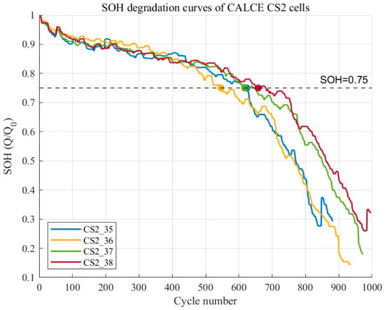
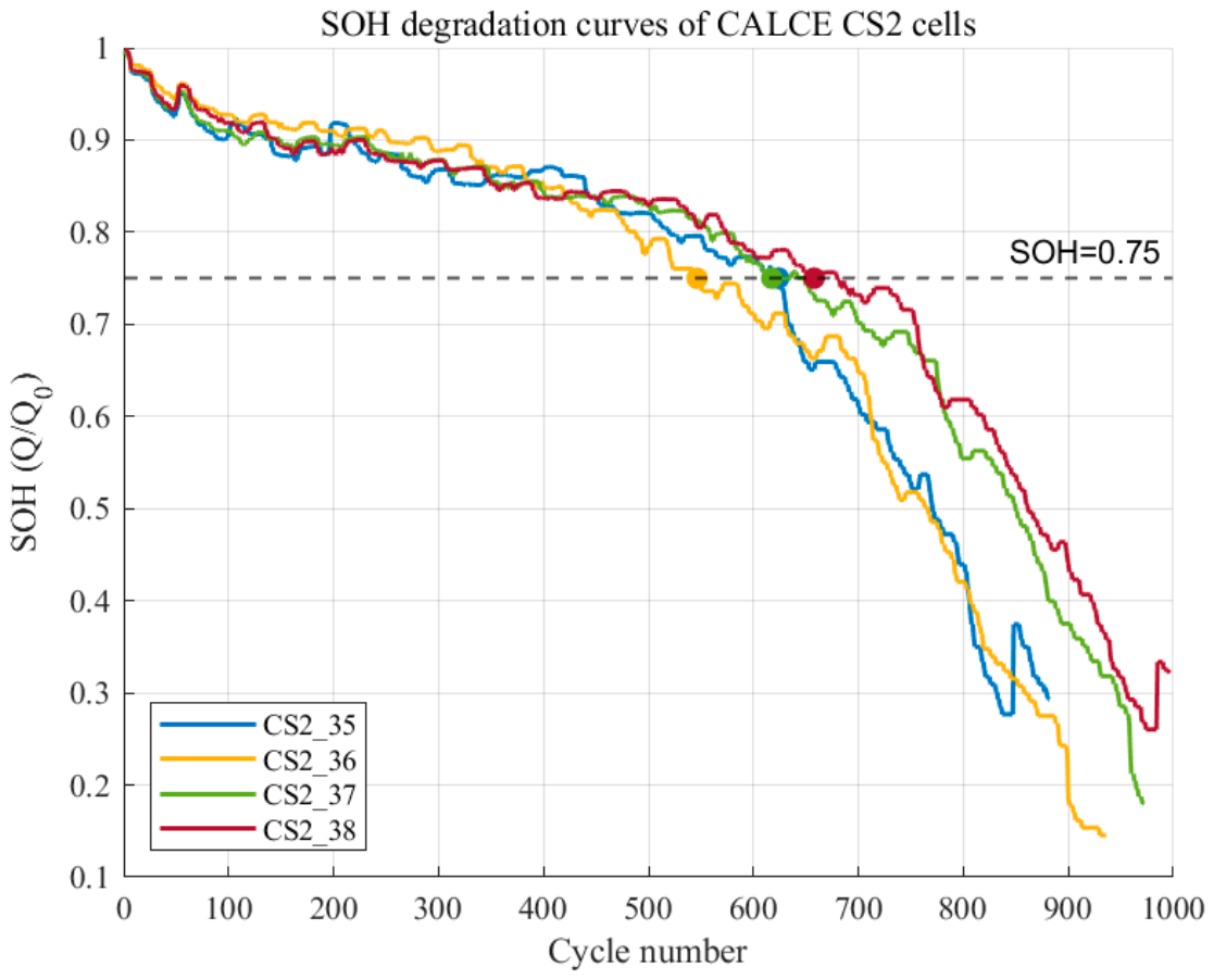
Q_i is the measured discharge capacity at cycle i and Q₀ is the discharge capacity at beginning of life. In this study, end-of-life is defined at a SOH threshold of 0.75. This threshold is used only as a descriptive reference for reporting degradation duration and the EOL statistics in Table 3. The predictive models in this work were trained to estimate continuous SOH values rather than a threshold-based EOL label. Therefore, changing the EOL threshold would change the interpreted crossing point on the SOH curve, but it would not alter the model structure, the regression target, or the fitted SOH trajectory itself. Besides the raw threshold-crossing cycle, we also computed a smoothed EOL to mitigate occasional measurement noise. The SOH trajectory is first smoothed using a moving-average filter with a five-cycle window, and the cycle index at which the smoothed SOH crosses 0.75 is obtained by linear interpolation. Both raw and smoothed EOL values are reported in Table 3 and are used only for a descriptive comparison of the degradation durations. Different applications may adopt different practical EOL criteria, but this does not change the formulation of the present SOH regression task. The SOH degradation curves of the four selected CS2 cells are shown in Figure 1.

Table 3. Summary of the CALCE CS2 cells used in this study.

Cell	Total Cycles (N)	Initial Capacity (Q0) (Ah)	EOL SOH = 0.75 (Raw)	EOL SOH = 0.75 (Smoothed)	Minimum SOH Observed
CS2_35	882	1.1264	622	623.8	0.228
CS2_36	936	1.1338	521	546.3	0.121
CS2_37	972	1.1243	615	617.6	0.179
CS2_38	996	1.1270	655	657.8	0.252

Figure 1. SOH degradation curves.

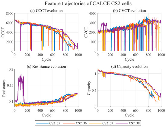
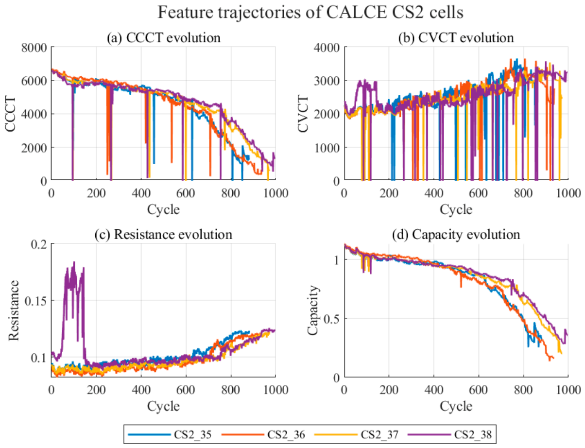
Rather than relying on high-dimensional curve representations, we used a compact set of cycle-level indicators that track degradation from complementary viewpoints. The constant-current charging time and constant-voltage charging time describe the evolution of charge acceptance and polarization during CC–CV charging. Internal resistance reflects the growth of ohmic and interfacial impedances with aging. Discharge capacity provides a direct measure of performance fade and is also used to compute SOH. In addition, we retained the scalar indicator k provided in the CALCE cycle-summary table as an auxiliary aging descriptor. In the released CSV files, k is reported as a single-valued cycle-level index and is used here as-is to enrich the low-dimensional feature space. Together, these variables form an interpretable yet learnable representation. Because long-term cycling records may contain occasional missing entries or abnormal spikes, the feature trajectories are screened using conservative consistency rules and simple cleaning, such as removing cycles with nonphysical values, to avoid injecting artificial trends. After cleaning, the features are normalized as described below to ensure stable optimization and fair contribution across dimensions. The trajectories of the selected cycle-level features are presented in Figure 2.

Figure 2. Feature trajectories.

Prior to feature construction, the CALCE cycle-summary tables were screened at the row level to identify abnormal cycle entries. In this study, the screening criterion was based on missing key fields in the selected descriptors. All flagged entries were removed before subsequent feature extraction and modeling. After screening, the numbers of removed cycle entries were 18 for CS2_35, 13 for CS2_36, 14 for CS2_37, and 10 for CS2_38. These removed entries corresponded to cycle-summary rows with missing key fields. This preprocessing was intended to eliminate incomplete records while preserving the overall chronological degradation trend of each battery. The removed cycle indices identified during preprocessing are summarized in Table 4.

Table 4. Removed abnormal cycle-summary entries in the CALCE dataset during preprocessing.

Battery	Number of Removed Entries	Removed Cycle Indices	Reason
CS2_35	18	96, 123, 141, 151, 162, 170, 318, 456, 582, 600, 698, 760, 827, 828, 832, 873, 874, 878	Missing key fields
CS2_36	13	107, 257, 379, 420, 523, 611, 661, 708, 719, 742, 783, 812, 935	Missing key fields
CS2_37	14	274, 276, 286, 307, 332, 436, 501, 565, 684, 738, 772, 794, 876, 881	Missing key fields
CS2_38	10	377, 450, 473, 558, 630, 653, 749, 767, 939, 983	Missing key fields

To avoid scale imbalance among heterogeneous features, min–max normalization was applied to each feature dimension using training-set statistics only. For a feature $x$, the normalized value $\tilde{x}$ is computed as:

$$\tilde{x}={\displaystyle \frac{x-x_{\mathrm{m}\mathrm{i}\mathrm{n}}}{x_{\mathrm{m}\mathrm{a}\mathrm{x}}-x_{\mathrm{m}\mathrm{i}\mathrm{n}}+\epsilon }}$$

(2)

where $x_{\mathrm{m}\mathrm{i}\mathrm{n}}$ and $x_{\mathrm{m}\mathrm{a}\mathrm{x}}$ are computed from the training portion of the data, and $\epsilon$ is a small constant to prevent numerical issues. At the inference time, the same parameters are used to transform test data, ensuring that no information from the test horizon leaks into preprocessing [15,16].

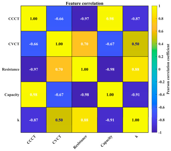
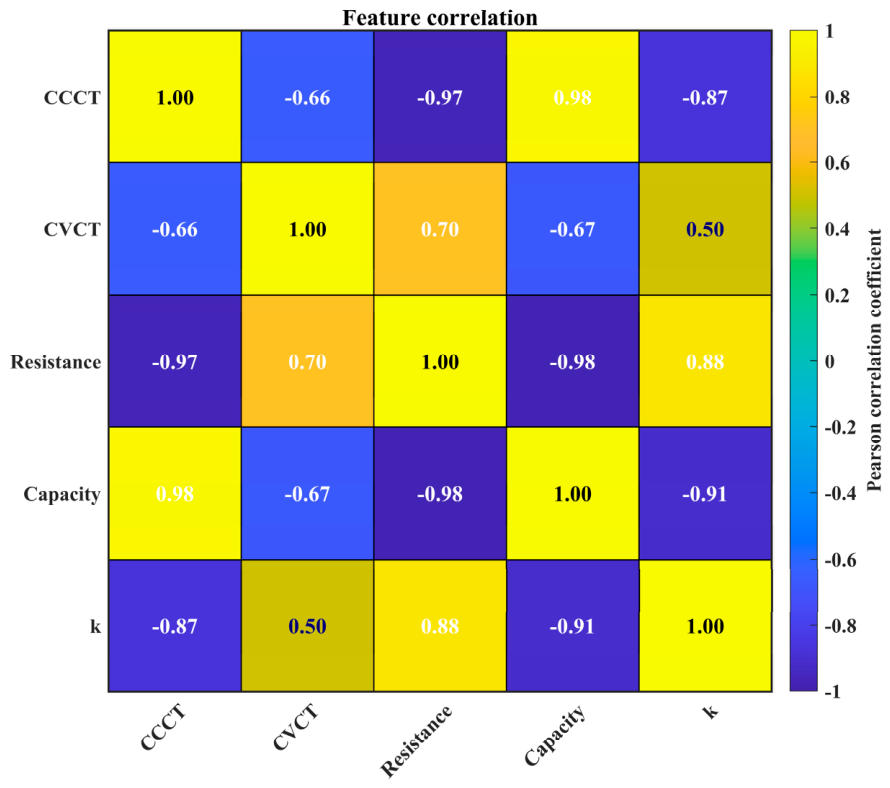
Although the five cycle-level indicators are all physically interpretable, they are not fully independent and may contain correlated information, as suggested by the feature-correlation analysis in Figure 3. Therefore, KPCA is introduced here not as an arbitrary dimensionality reduction step, but as a compact feature-transformation method to reduce redundancy and control input complexity for limited single-cell degradation data. In this study, the first three KPCA components were retained as a practical compromise between information retention and representation compactness, rather than as a claim that three-dimensional representation is universally optimal for all SOH datasets.

Figure 3. Feature correlation.

SOH forecasting is cast as a supervised learning task on a cycle-ordered feature sequence with a fixed look-back window. The normalized feature vector at cycle t is denoted by xt and has dimension d, corresponding to the selected indicators CCCT, CVCT, resistance, capacity, and k. The window length L is set to 8 cycles. For each time index t, the input sample X_t stacks the most recent L feature vectors, and the target is the SOH at cycle t + 1, as defined in Equations (3) and (4). The model learns the mapping from X_t to the one-step-ahead SOH shown in Equation (5).

$${\mathbf{X}}_t=[xt-m+1,xt-m+2,\dots ,xt]$$

(3)

and the corresponding one-step-ahead target is:

$$y_t={\mathrm{S}\mathrm{O}\mathrm{H}}_{t + 1}$$

(4)

Thus, the learning task is to approximate the mapping:

$${\widehat{y}}_t=f\left({\mathbf{X}}_t\right)$$

(5)

where $f(\cdot )$ denotes a predictive model.

In Equation (5), f_θ denotes the predictive model with parameters θ. Section 2.2, Section 2.3, Section 2.4 and Section 2.5 instantiate f_θ using the KPCA–BP baseline, CNN–LSTM, the fixed-hyperparameter attention–LSTM baseline, and the hyperparameter-adaptive model Ada-TL.

After constructing sliding-window samples, the sequence is split chronologically: the first 70% of samples are used for training and the remaining 30% are reserved for testing, without random shuffling. The same split boundary is applied to all compared models so that performance differences reflect modeling choices rather than data partitioning.

2.2. BP Network

As a lightweight baseline, we adopted a KPCA–BP pipeline [17,18]. From the cycle-summary table, we extracted five scalar indicators: CCCT, CVCT, resistance, discharge capacity, and k. Discharge capacity is normalized by the initial capacity to obtain SOH. KPCA is applied to the five-indicator set to obtain a lower-redundancy representation of the cycle-level aging information, and the first three kernel principal component scores are retained. This choice is intended to balance information preservation and representation compactness for the limited single-cell dataset used in this study. For each cycle t, we combined these three scores with the corresponding SOH to form a four-dimensional vector. Training samples are created with a 8-cycle look-back window and a one-step forecasting horizon. The BP input consists of the vectors from the past 8 cycles, together with the three component scores at the next cycle as exogenous information, and the output is the SOH at the next cycle. This construction yields a 35-dimensional input and a scalar regression target.

The BP regressor learns a nonlinear mapping from the constructed input vector to the next-cycle SOH, as summarized in Equation (6). All inputs and targets are normalized to [0, 1] using min–max scaling fitted on the training portion only. The same scaling parameters are reused for test inference, and predictions are inverse-transformed back to the SOH scale for evaluation.

$${\widehat{y}}_{t + \Delta }=\mathrm{M}\mathrm{L}\mathrm{P}\left(\mathrm{v}\mathrm{e}\mathrm{c}\left({\mathbf{Z}}_t\right)\right)$$

(6)

where $\mathrm{v}\mathrm{e}\mathrm{c}(\cdot )$ concatenates the windowed KPCA components into a single vector. We adopted a shallow multilayer perceptron with two hidden layers. We used a two-hidden-layer multilayer perceptron with 32 and 16 neurons, tan-sigmoid activations, and a linear output layer. Parameters were optimized with Adam for up to 5000 epochs using an initial learning rate of 0.01. Training minimized the mean squared error with an early-stopping tolerance of 1 × 10⁻⁶. Preprocessing steps, including normalization and window construction, were kept identical across models to ensure a fair comparison.

2.3. CNN–LSTM

BP operates on flattened vectors and does not explicitly model temporal locality. To capture both short-range variations and longer-range degradation memory, we adopted a CNN–LSTM [19] architecture in which a temporal convolutional front-end extracts local patterns and an LSTM regressor summarizes the sequence into a degradation-aware representation. The CNN front-end is introduced to extract short-range local variations, while the downstream LSTM summarizes the resulting sequence into a degradation-aware temporal representation. Each sample starts from the same 8-cycle window used above. We represented the window as a length-8 multivariate sequence with four channels, namely the three KPC scores and the SOH value at each cycle.

The convolutional front-end maps the input sequence to a set of local features through a temporal convolution followed by a nonlinear activation, which can be written as

$$H=\sigma (W\ast X+b)$$

(7)

In Equation (7), $\mathit{X}$ denotes the input sequence to the convolutional block, and its elements ${\mathit{X}}_{\mathit{t}}\in {\mathbb{R}}^4$ correspond to the four-channel feature vector at time step $\mathit{t}$ within the 8-step sequence. The symbol “$\ast$” denotes one-dimensional convolution along the time axis. The matrix $\mathit{W}$ represents the learnable convolutional kernel parameters, and $\mathit{b}$ is the corresponding bias term. The function $\mathit{\sigma }(\cdot )$ denotes the element-wise nonlinear activation used after convolution. The output $\mathit{H}$ denotes the learned local representation produced by the convolutional block, where ${\mathit{H}}_{\mathit{t}}$ is the feature vector at time step $\mathit{t}$ after temporal convolution [20]. In the implemented CNN block, two convolutional layers are used. Both layers adopt a kernel size of [2, 1] and a stride of [1, 1]. The numbers of filters are 32 and 64 for the first and second convolutional layers, respectively, and each convolutional layer is followed by a ReLU activation. The extracted features are then flattened and passed to an LSTM layer with 50 hidden units. Because the input window in this study was short, the convolutional configuration was intentionally kept conservative: the small kernel and unit stride preserve local temporal transitions, while the progressive increase in filter number improves the local feature extraction without introducing an excessively large receptive field.

The LSTM then consumes the convolutional features and accumulates temporal memory over the window. For each time step $\mathit{\tau }$, the LSTM receives the current input vector ${\mathit{x}}_{\mathit{\tau }}$ (i.e., the convolutional feature at time step $\mathit{\tau }$) [21] and updates its hidden state ${\mathit{h}}_{\mathit{\tau }}$ by the standard gating mechanism:

$$i_{\tau }=\sigma (W_i{h}_{\tau - 1}+U_i{x}_{\tau }+b_i)$$

(8)

$$f_{\tau }=\sigma \left(W_f{h}_{\tau - 1}+U_f{x}_{\tau }+b_f\right)$$

(9)

$${\tilde{c}}_{\tau }=\mathrm{t}\mathrm{a}\mathrm{n}\mathrm{h}(W_c{h}_{\tau - 1}+U_c{x}_{\tau }+b_c)$$

(10)

$$c_{\tau }=f_{\tau }\odot c_{\tau - 1}+i_{\tau }\odot {\tilde{c}}_{\tau }$$

(11)

$$o_{\tau }=\sigma (W_o{h}_{\tau - 1}+U_o{x}_{\tau }+b_o)$$

(12)

$$h_{\tau }=o_{\tau }\odot tanh\left(c_{\tau }\right)$$

(13)

In Equations (8)–(13), ${\mathit{x}}_{\mathit{\tau }}$ denotes the LSTM input at step $\mathit{\tau }$, which is the convolutional feature vector extracted from the temporal CNN. The vector ${\mathit{h}}_{\mathit{\tau } - \mathbf{1}}$ is the previous hidden state, and ${\mathit{h}}_{\mathit{\tau }}$ is the updated hidden state at step $\mathit{\tau }$. The scalar $\mathit{\tau }$ indexes time steps within the 8-step window. The vectors ${\mathit{i}}_{\mathit{\tau }}$, ${\mathit{f}}_{\mathit{\tau }}$, and ${\mathit{o}}_{\mathit{\tau }}$ are the input gate, forget gate, and output gate, respectively, and ${\mathit{c}}_{\mathit{\tau }}$ denotes the LSTM cell state. The vector ${\tilde{\mathit{c}}}_{\mathit{\tau }}$ is the candidate cell update computed from the current input and the previous hidden state. The matrices ${\mathit{W}}_{\mathit{i}},{\mathit{W}}_{\mathit{f}},{\mathit{W}}_{\mathit{c}},{\mathit{W}}_{\mathit{o}}$ are the learnable weight matrices associated with the previous hidden state, and ${\mathit{U}}_{\mathit{i}},{\mathit{U}}_{\mathit{f}},{\mathit{U}}_{\mathit{c}},{\mathit{U}}_{\mathit{o}}$ are the learnable weight matrices associated with the current input. The vectors ${\mathit{b}}_{\mathit{i}},{\mathit{b}}_{\mathit{f}},{\mathit{b}}_{\mathit{c}},{\mathit{b}}_{\mathit{o}}$ are the corresponding bias terms. The operator $\odot$ denotes element-wise multiplication. The function $\mathit{\sigma }(\cdot )$ is the logistic sigmoid activation, and $\mathit{t}\mathit{a}\mathit{n}\mathit{h}(\cdot )$ is the hyperbolic tangent activation.

Finally, a fully connected regression head maps the last hidden state ${\mathit{h}}_{\mathit{T}}$ (with $\mathit{T}=\mathbf{11}$ time steps) to the SOH prediction ${\widehat{\mathit{y}}}_{\mathit{t} + \mathit{\Delta }}$, where $\mathbf{\Delta }=\mathbf{1}$ corresponds to the one-step-ahead forecast.

This design is practically motivated. The temporal convolution helps suppress high-frequency disturbances by extracting local patterns, while the LSTM aggregates information across the window to form a degradation-aware state. Consequently, compared with BP, the CNN–LSTM model is expected to be more robust when the feature trajectories exhibit short-term fluctuations.

2.4. LSTM Baseline with Attention

CNN–LSTM emphasizes locality, but battery degradation also exhibits non-local dependencies across cycles. To capture global relations within a window, we built an attention-enhanced LSTM baseline that combines a Transformer-style encoder with an LSTM regressor. For brevity, this model is referred to as the LSTM baseline [22] in the remainder of the paper. The attention mechanism is used to capture non-local interactions within the input window, whereas the LSTM maps the encoded sequence into a temporally coherent degradation state. Each sample is represented as a length-$k$ sequence with four channels, where $k=10$ and each time step contains three KPCA components and the corresponding SOH. A linear projection maps the four-dimensional vector at each time step to an embedding of dimension $d_{\mathrm{model}}=24$. Stacking the embeddings over the window yields the embedded input sequence $E\in {\mathbb{R}}^{k \times d_{\mathrm{model}}}$, where each row of $E$ is the token embedding of one cycle within the window [23].

The Transformer encoder block starts by forming the query, key, and value matrices via learnable linear projections of $E$. Specifically, $Q=E{W}_Q$, $K=E{W}_K$, and $V=E{W}_V$, where $W_Q$, $W_K$, and $W_V$ are learnable projection matrices. Multi-head attention uses $h=4$ parallel heads, so the per-head key dimension is $d_k=d_{\mathrm{model}}/h$. For a given head, scaled dot-product attention is computed as

$$\mathrm{A}\mathrm{t}\mathrm{t}\mathrm{e}\mathrm{n}\mathrm{t}\mathrm{i}\mathrm{o}\mathrm{n}(\mathbf{Q},\mathbf{K},\mathbf{V})=\mathrm{s}\mathrm{o}\mathrm{f}\mathrm{t}\mathrm{m}\mathrm{a}\mathrm{x}\left({\displaystyle \frac{\mathbf{Q}{\mathbf{K}}^{\mathrm{\top }}}{\sqrt{d_k}}}\right)\mathbf{V}$$

(14)

where $Q$, $K$, and $V$ denote the query, key, and value matrices of that head. The product $Q{K}^{\mathrm{\top }}$ produces pairwise similarity scores between time steps, and the scaling term $\sqrt{d_k}$ stabilizes the magnitude of the scores when $d_k$ increases. The function $\mathrm{s}\mathrm{o}\mathrm{f}\mathrm{t}\mathrm{m}\mathrm{a}\mathrm{x}(\cdot )$ is applied along the key/time dimension so that each row of the resulting attention-weight matrix sums to one. The right multiplication by $V$ yields the weighted aggregation of value vectors and produces the attention output for each time step.

The outputs of the $h$ attention heads are then concatenated and projected back to the embedding space:

$$\mathrm{M}\mathrm{H}\mathrm{A}\left(\mathbf{E}\right)=\mathrm{C}\mathrm{o}\mathrm{n}\mathrm{c}\mathrm{a}\mathrm{t}({\mathrm{head}}_1,\dots ,{\mathrm{head}}_h){\mathbf{W}}_O$$

(15)

where ${\mathrm{h}\mathrm{e}\mathrm{a}\mathrm{d}}_j$ denotes the attention output computed by Equation (9) in the $j$-th head using its own learned projections, $\mathrm{C}\mathrm{o}\mathrm{n}\mathrm{c}\mathrm{a}\mathrm{t}(\cdot )$ denotes concatenation along the feature dimension, and $W_O$ is the learnable output projection matrix that maps the concatenated representation to dimension $d_{\mathrm{model}}$.

The encoder adopts a pre-normalization design. Layer normalization is applied to the sub-layer input before self-attention and before the feed-forward network, and each sub-layer output is added back to its corresponding input through a residual connection. A dropout layer with rate $p=0.1$ is applied to the output of the self-attention sub-layer and the feed-forward sub-layer before the residual addition, which helps reduce overfitting while preserving the residual pathway. The position-wise feed-forward network is defined as:

$$\mathrm{F}\mathrm{F}\mathrm{N}\left(\mathbf{x}\right)={\mathbf{W}}_2 \varphi ({\mathbf{W}}_1\mathbf{x}+{\mathbf{b}}_1)+{\mathbf{b}}_2$$

(16)

where $x$ denotes the input vector at a given time step, $W_1\in {\mathbb{R}}^{d_{\mathrm{model}} \times d_{\mathrm{ff}}}$ and $W_2\in {\mathbb{R}}^{d_{\mathrm{ff}} \times d_{\mathrm{model}}}$ are learnable weight matrices, $b_1$ and $b_2$ are bias vectors, $d_{\mathrm{ff}}=128$ is the feed-forward dimension, and $\varphi (\cdot )$ is the element-wise activation function used in the feed-forward network.

After the Transformer encoder, the LSTM regressor receives the encoded sequence and consolidates it into a temporally consistent degradation state. The LSTM uses 32 hidden units and outputs the representation from the last time step of the window. A fully connected regression layer maps this last hidden representation to the one-step-ahead SOH estimate ${\widehat{y}}_{t + \Delta }$, where $\Delta =1$ denotes one-step-ahead prediction.

Hyperparameters are fixed for this baseline: $d_{\mathrm{model}}=64$, $h=4$, $d_{\mathrm{ff}}=128$, dropout rate $p=0.1$, and 32 LSTM units. Training uses Adam for 300 epochs with an initial learning rate of $1\times {10}^{-3}$. The learning rate is reduced by a factor of 0.1 every 200 epochs. The gradient threshold is set to 1, and the $L_2$ regularization coefficient is $1\times {10}^{-3}$. The same chronological split is used for all models to ensure a fair comparison.

2.5. Adaptive Hyperparameter Tuning for Transformer–LSTM

Model performance depends strongly on architectural and regularization hyperparameters. To reduce manual trial-and-error, we endowed the attention–LSTM baseline with an adaptive hyperparameter tuning strategy, forming an automated configuration-search framework termed Ada-TL. The optimizer is employed to adapt a small set of high-impact hyperparameters so that the model configuration better matches cell-dependent degradation patterns. The optimizer tunes three hyperparameters while keeping the remaining architectural settings fixed to constrain the search space. Specifically, the tunable hyperparameters are collected in a vector $\theta$, including the number of attention heads $H$, the initial learning rate ${\eta }_0$ used by Adam, and the $L_2$ regularization coefficient $\lambda$. To keep per-head representation comparable across different head configurations, we set the embedding dimension to $d_{\mathrm{model}}=8H$. Under this design, the per-head key dimension satisfies $d_k=d_{\mathrm{model}}/H=8$, so changing $H$ alters the number of heads without changing per-head dimensionality. The search ranges are $H\in [2, 8]$, ${\eta }_0\in [0.001, 0.01]$, and $\lambda \in [0.0001, 0.001]$. During optimization, $H$ is updated as a real variable and then rounded to the nearest integer and clipped to $[2, 8]$, whereas ${\eta }_0$ and $\lambda$ remain continuous and are clipped to their respective bounds. These intervals are chosen as a practically meaningful search domain rather than as an exhaustive global search space, with the aim of balancing model flexibility, optimization stability, computational cost, and the limited scale of the dataset. Very small or excessively large values outside these intervals were not emphasized in this study because the goal of Ada-TL is to perform stable adaptive tuning of a few high-impact parameters, not unrestricted architecture discovery. For each candidate $\theta$, we instantiated the attention–LSTM network by setting $d_{\mathrm{model}}=8H$ and using fixed settings for the remaining architecture (feed-forward dimension, dropout rate, and the number of LSTM units). The candidate learning rate ${\eta }_0$ and regularization coefficient $\lambda$ are passed to the Adam optimizer. The candidate network is trained for 70 epochs. For each candidate hyperparameter vector, the model is trained on the training split and evaluated on a chronologically subsequent validation split. The validation RMSE is used as the fitness value during optimization, while the held-out test split is used only for final performance reporting; the same chronological train/test boundary described in Section 2.1 was applied consistently across all models.

$$\mathrm{f}\mathrm{i}\mathrm{t}(\mathit{\theta })=\sqrt{{\displaystyle \frac{1}{N}}\sum _{i = 1}^N(y_i-{\widehat{y}}_i{)}^2}$$

(17)

In Equation (17), $N$ denotes the number of samples in the evaluation split, $y_i$ denotes the ground-truth SOH of sample $i$, and ${\widehat{y}}_i$ denotes the predicted SOH produced by the candidate model under $\theta$. The optimizer seeks to minimize $\mathrm{f}\mathrm{i}\mathrm{t}\left(\theta \right)$, and the best fitness value at each iteration was recorded for subsequent convergence analysis. The optimizer maintains a population of $n_{\mathrm{pop}}=10$ candidate solutions and runs for $T=20$ iterations. Each candidate is represented by a position vector $X_i$ that encodes the three components of $\theta$, namely $X_i=[H,{\eta }_0,\lambda ]$. Let $X_{\mathrm{best}}$ denote the best candidate position in the current population (lowest fitness) and $X_{\mathrm{worst}}$ denote the worst candidate position (highest fitness). At iteration $t$, a time-varying control factor $M$ is computed to regulate the exploration–exploitation balance, and $M$ decreases as the search proceeds so that the update gradually shifts from exploration to exploitation.

$$M={\left(1−{\displaystyle \frac{t}{T}}\right)}^2$$

(18)

Based on $M$, the optimizer alternates between two main moves. Elliptic exploration searches around the current best solution using an ellipse-shaped update rule, where random coefficients and a phase term preserve diversity and encourage broader exploration in early iterations.

$${\mathbf{X}}_i^{\prime }={\mathbf{X}}_{\mathrm{best}}+a\mathrm{c}\mathrm{o}\mathrm{s}\left(\theta \right)({\mathbf{X}}_{\mathrm{best}}-{\mathbf{X}}_i)+b\mathrm{s}\mathrm{i}\mathrm{n}\left(\theta \right)({\mathbf{X}}_{\mathrm{best}}-{\mathbf{X}}_i)$$

(19)

In Equation (19), $X_i$ is the current position of candidate $i$ and $X_i^{\prime }$ is the updated position. The scalars $a$ and $b$ are sampled uniformly from [0, 2], and the phase $\phi$ is sampled uniformly from [0, 2]. Spiral exploitation tightens candidates toward the current best position through a spiral-like move, where the contraction strength is modulated by $M$ and becomes progressively stronger as M decreases.

$${\mathbf{X}}_i^{\prime }={\mathbf{X}}_{\mathrm{best}}+\mathrm{e}\mathrm{x}\mathrm{p}\left(0.5M\right)\mathrm{c}\mathrm{o}\mathrm{s}\left(2\pi u\right)({\mathbf{X}}_{\mathrm{best}}-{\mathbf{X}}_i)$$

(20)

In Equation (20), $u$ is sampled uniformly from [0, 1]. To further improve robustness and reduce stagnation, two occasional perturbations are applied. Collision perturbation stretches candidates away from poor regions using the direction from the worst to the best solution, which helps the population escape from stagnant states.

$${\mathbf{X}}_i^{\prime }\leftarrow {\mathbf{X}}_i^{\prime }+r({\mathbf{X}}_{\mathrm{best}}-{\mathbf{X}}_{\mathrm{worst}})$$

(21)

In Equation (21), $r$ is sampled uniformly from [0, 1]. Lévy-flight refinement injects heavy-tailed jumps to reduce the risk of local minima. With probability $p_L$, the following update is applied:

$${\mathbf{X}}_i^{\prime }\leftarrow {\mathbf{X}}_i^{\prime }+\alpha \cdot \mathrm{L}\mathrm{e}\mathrm{v}\mathrm{y}\left(\beta \right)\odot ({\mathbf{X}}_i^{\prime }-{\mathbf{X}}_{\mathrm{best}})$$

(22)

In Equation (22), $\alpha$ is a step-size coefficient, $\mathrm{L}\mathrm{e}\mathrm{v}\mathrm{y}\left(\beta \right)$ denotes a Lévy-distributed random vector controlled by exponent $\beta$, and $\odot$ denotes element-wise multiplication. After each update, variables are clipped to their bounds; $H$ is then rounded to the nearest integer and clipped to $[2, 8]$. The best solution is updated whenever a lower fitness value is found, and the optimizer returns the best hyperparameter set $\theta$ together with the convergence record. After the search terminates, the best hyperparameter set ${\theta }^{\backslash *}$ is used to retrain Ada-TL for final reporting. The retraining uses Adam for 300 epochs, with the initial learning rate set to ${\eta }_0$, a piecewise decay by a factor of 0.1 every 200 epochs, a gradient threshold of 1, and $L_2$ regularization set to $\lambda$.

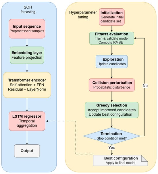
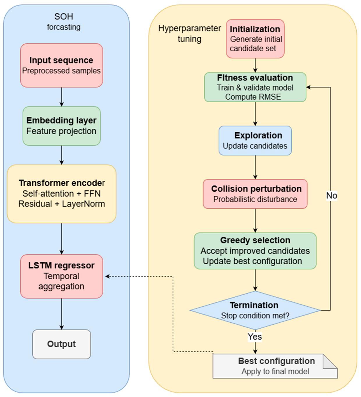
From a functional perspective, the effectiveness of Ada-TL comes from how four elements work together: compact representation, non-local dependency extraction, sequential memory formation, and adaptive optimization. The compact health-indicator sequence reduces redundant information in cycle-level measurements and makes the learning target less noisy. The Transformer encoder relates the current degradation state to earlier observations within the input window instead of using only adjacent samples. The LSTM then converts the encoded sequence into a temporally ordered degradation memory. Finally, the adaptive tuning stage adjusts the key training-related hyperparameters according to the degradation characteristics of different cells. In practical deployment, the hyperparameter search and model training stages are performed offline. After the best configuration is identified, online application only requires forward inference with the trained predictor, rather than repeated optimization during operation. The overall workflow of the proposed Ada-TL model is illustrated in Figure 4.

Figure 4. The flowchart of the Ada-TL model.

3. Results and Discussion

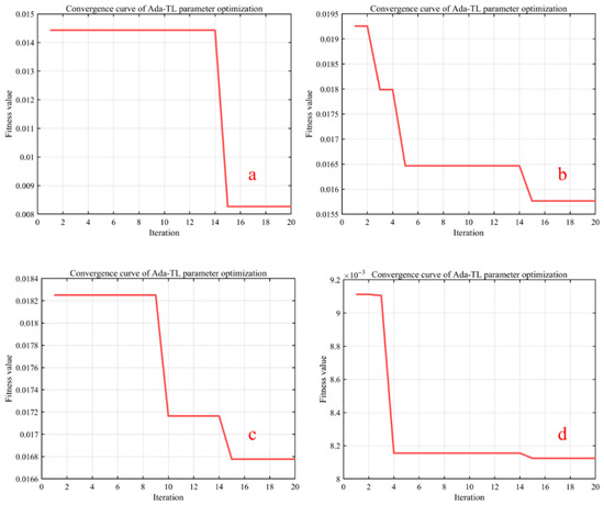
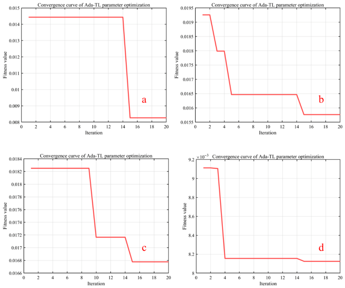
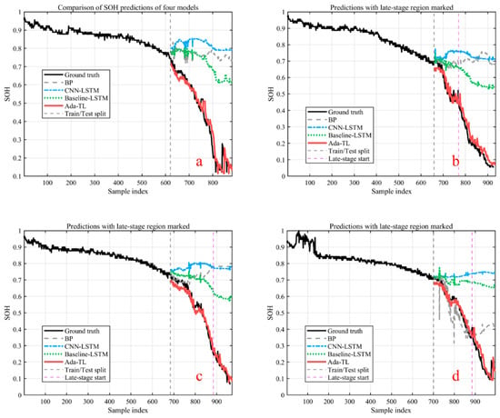
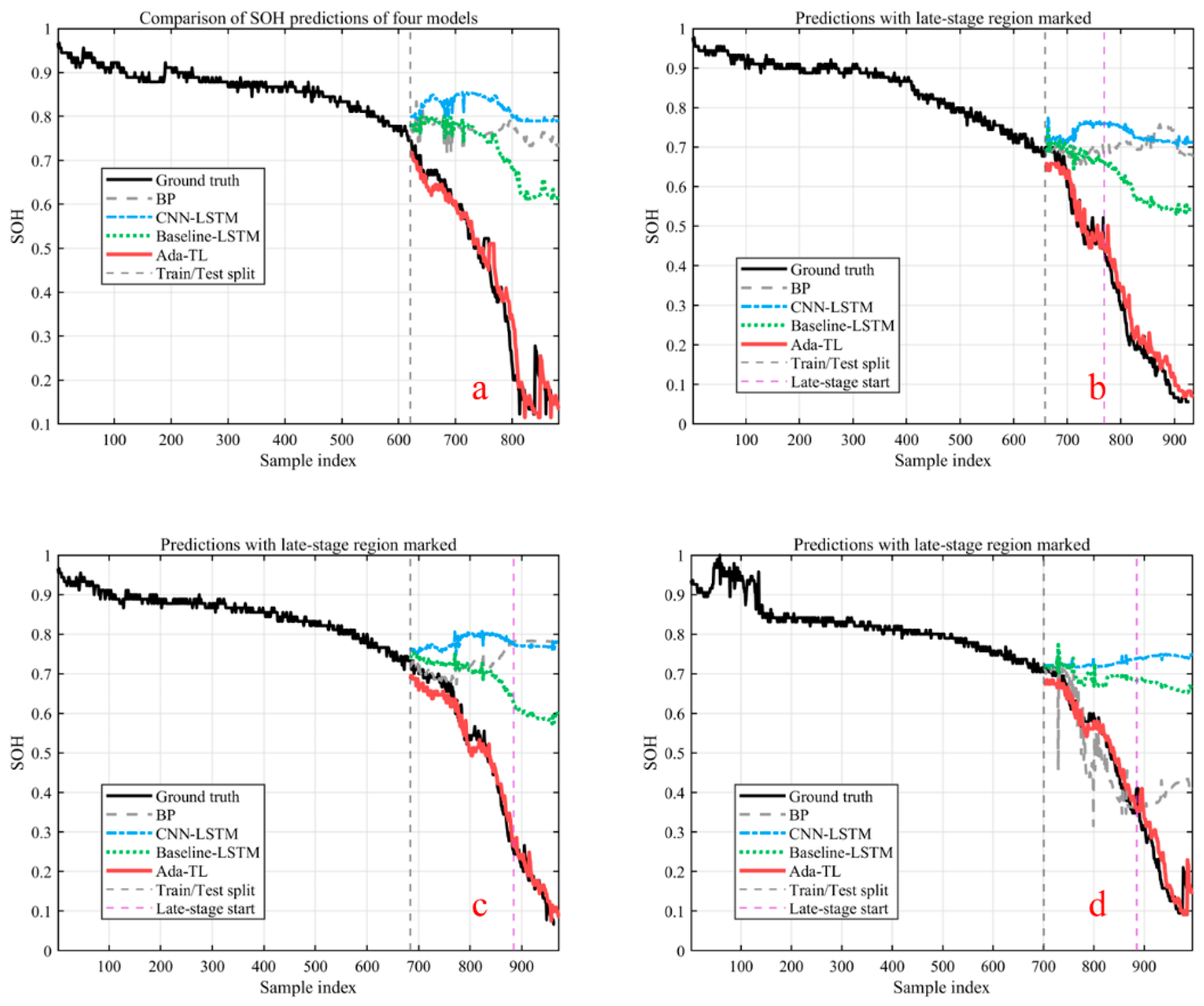
To evaluate the proposed framework under a more rigorous and practically meaningful setting, all comparative experiments were re-conducted using a chronological 70:30 train–test split. In this configuration, the first 70% of each degradation trajectory was used for model development, whereas the remaining 30% was reserved for out-of-sample evaluation without random shuffling. Compared with a looser partition, this setting exposes each model to a longer unseen degradation horizon and therefore provides a more demanding test of generalization. Four models were compared, namely BP, CNN–LSTM, the fixed-hyperparameter Baseline–LSTM, and the proposed Ada-TL. Unless otherwise stated, the subplots in Figure 5, Figure 6, Figure 7 and Figure 8 correspond to (a) CS2_35, (b) CS2_36, (c) CS2_37, and (d) CS2_38.

Figure 5. Convergence curves of the adaptive hyperparameter optimization: (a) CS2_35; (b) CS2_36; (c) CS2_37; (d) CS2_38.

Figure 6. SOH prediction of the four models: (a) CS2_35; (b) CS2_36; (c) CS2_37; (d) CS2_38.

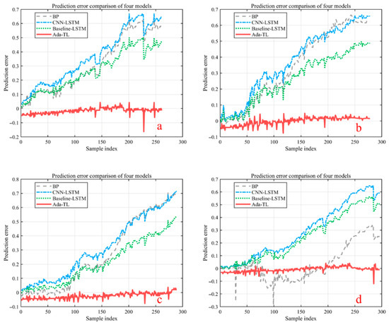
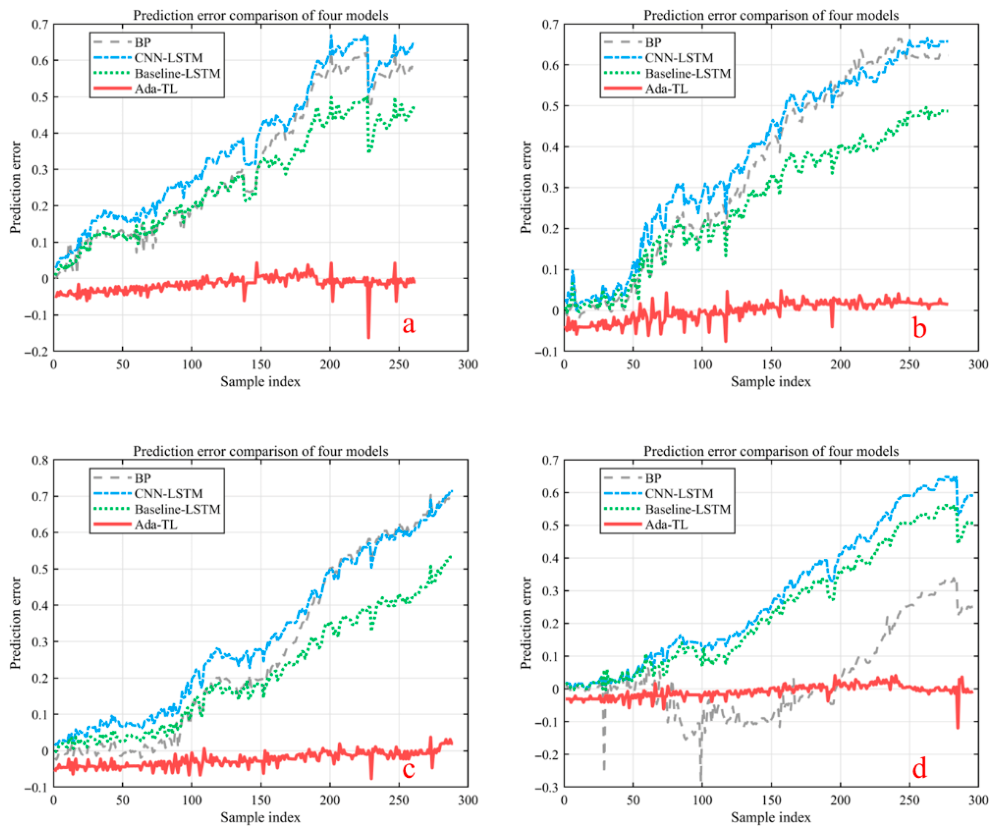
Figure 7. Prediction error comparison of the four models: (a) CS2_35; (b) CS2_36; (c) CS2_37; (d) CS2_38.

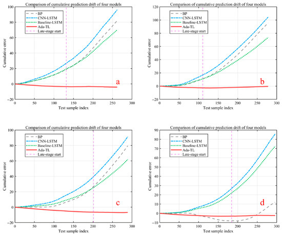
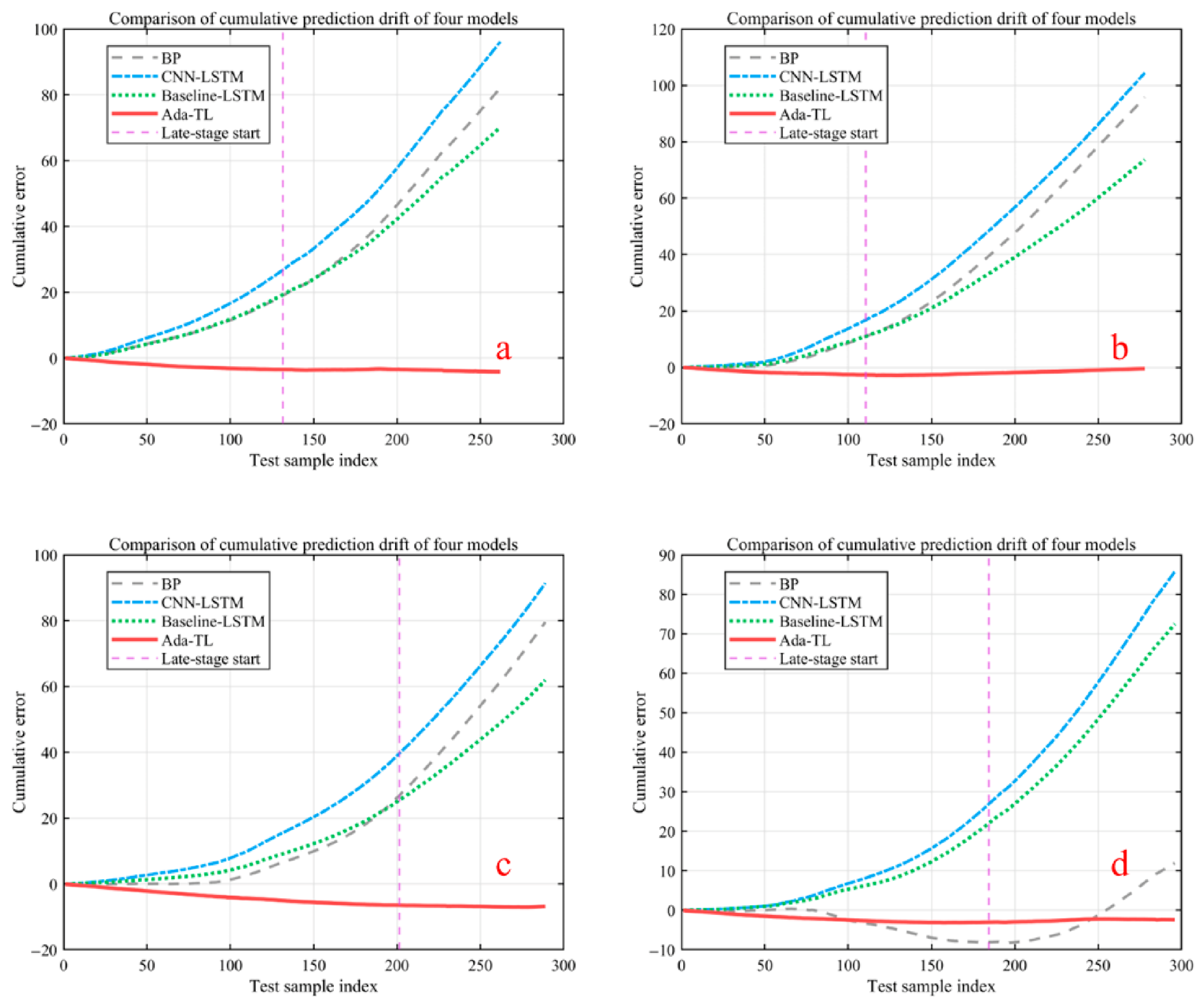
Figure 8. Cumulative prediction drift of the four models for four CS2 cells: (a) CS2_35; (b) CS2_36; (c) CS2_37; (d) CS2_38.

3.1. Overall SOH Prediction Performance Under the Chronological 70:30 Split

Figure 5 shows the convergence curves of the adaptive hyperparameter optimization process for the four cells. Although the final fitness values differed across cells, all cases exhibited a similar pattern, characterized by a rapid early decrease followed by gradual stabilization. This indicates that the search procedure is able to identify suitable hyperparameter combinations within a limited number of iterations and remains numerically stable under different degradation trajectories. The convergence behavior also supports the use of adaptive tuning as a data-driven and reproducible configuration mechanism under different degradation trajectories.

The predicted SOH trajectories are compared in Figure 6, and the corresponding overall test-set metrics are summarized in Table 5, Table 6 and Table 7. A consistent performance ranking can be observed across the four cells. BP showed limited temporal consistency and tended to deviate substantially once the degradation curve entered the accelerated decline region. CNN–LSTM performed even less favorably in most cases, with larger systematic overestimation and a wider deviation band over the unseen horizon. The Baseline–LSTM improved the smoothness of the predicted trajectory and generally outperformed BP and CNN–LSTM, indicating that attention-enhanced sequence modeling is beneficial for SOH forecasting. However, under the stricter chronological 70:30 split, Ada-TL achieved the best overall performance on all four cells in terms of RMSE, MAE, and MAPE, which confirms that the proposed adaptive tuning strategy improves generalization rather than merely fitting a particular segment of the degradation curve.

Table 5. RMSE of SOH prediction for CS2 batteries.

Battery	BP	CNN–LSTM	Baseline–LSTM	Ada-TL
CS2_35	0.3687	0.4137	0.3031	0.0264
CS2_36	0.4135	0.4308	0.3075	0.0242
CS2_37	0.3703	0.3825	0.2662	0.0310
CS2_38	0.1424	0.3587	0.3068	0.0210

Table 6. MAE of SOH prediction for CS2 batteries.

Battery	BP	CNN–LSTM	Baseline–LSTM	Ada-TL
CS2_35	0.3132	0.3669	0.2676	0.0200
CS2_36	0.3451	0.3757	0.2649	0.0200
CS2_37	0.2775	0.3162	0.2141	0.0262
CS2_38	0.1028	0.2897	0.2450	0.0163

Table 7. MAPE of SOH prediction for CS2 batteries.

Battery	BP	CNN–LSTM	Baseline–LSTM	Ada-TL
CS2_35	130.38	145.66	106.52	4.92
CS2_36	259.48	268.99	194.03	9.30
CS2_37	144.04	149.66	104.87	6.34
CS2_38	53.16	135.85	116.09	4.17

For CS2_35, Ada-TL reduced the RMSE, MAE, and MAPE to 0.0264, 0.0200, and 4.92%, respectively, whereas the corresponding values of the Baseline–LSTM remained at 0.3031, 0.2676, and 106.52%. The same trend was observed for CS2_36, where Ada-TL achieved 0.0242 RMSE, 0.0200 MAE, and 9.30% MAPE, again substantially lower than the competing models. For CS2_37, although the Baseline–LSTM remained the strongest conventional baseline, Ada-TL still lowered the error to 0.0310 RMSE, 0.0262 MAE, and 6.34% MAPE. For CS2_38, the proposed model reached 0.0210 RMSE, 0.0163 MAE, and 4.17% MAPE, clearly outperforming BP, CNN–LSTM, and the fixed-hyperparameter baseline. These results show that the proposed model is not only competitive on one specific cell, but maintains clear superiority across all four degradation trajectories when evaluated under the same chronological split.

The error evolution shown in Figure 7 further clarifies the source of this improvement. CNN–LSTM exhibited the largest positive error over extended portions of the test region, indicating a persistent tendency to overestimate SOH. BP also showed strong fluctuation and poor temporal smoothness, which is consistent with its flattened-input formulation and limited sequence modeling capability. The Baseline–LSTM narrowed the error band but still accumulated visible deviation on several cells, especially when the unseen horizon became longer. In contrast, Ada-TL kept the prediction error closer to zero throughout most of the test interval and showed a substantially narrower fluctuation band. This behavior suggests that the advantage of Ada-TL is not restricted to a few isolated prediction points; instead, it reflects more stable error control along the full trajectory.

The predicted SOH trajectories are compared in Figure 6, and the corresponding overall test-set metrics are summarized in Table 5 for RMSE, Table 6 for MAE, and Table 7 for MAPE. The superiority is reflected not only in lower scalar metrics, but also in the shape of the predicted trajectory and the temporal evolution of the prediction error. This point is important because it shows that the proposed framework retains accuracy even when the unseen test interval extends well beyond the training horizon, which is closer to the actual deployment condition of battery health prediction models.

3.2. Late-Stage Prediction Accuracy and Cumulative Drift Analysis

Although the overall test-set metrics in Table 5, Table 6 and Table 7 already show the clear superiority of Ada-TL, scalar errors computed over the full unseen horizon do not completely reflect model behavior in the most practically critical part of the degradation trajectory. In battery SOH forecasting, the later stage is more challenging because the degradation slope often changes more rapidly and the cumulative effect of sequential prediction bias becomes more pronounced. To further examine model robustness, an additional late-stage analysis was conducted together with a cumulative signed error assessment.

The late-stage region was defined according to the post-processing criterion used in the comparative evaluation. Specifically, the turning-point information of the degradation trajectory was first examined. When the knee point was located inside the test interval, the post-knee part of the test set was used as the late-stage region; otherwise, the last 30% of the test set was adopted. This definition ensures that the analysis focused on the most demanding part of the unseen degradation trajectory while remaining consistent across cells with different aging patterns.

Table 8 summarizes the late-stage MAE, RMSE, MAPE, and MBE of the four models. A highly consistent trend was observed. For all four cells, Ada-TL achieved the lowest late-stage MAE, RMSE, and MAPE. On CS2_35, the late-stage RMSE of Ada-TL was 0.0217, compared with 0.4967 for BP, 0.5418 for CNN–LSTM, and 0.3974 for the Baseline–LSTM. On CS2_36, Ada-TL further reduced the late-stage RMSE to 0.0191, again remaining far below the competing methods. The same pattern holds for CS2_37 and CS2_38, where the late-stage RMSE values of Ada-TL were 0.0169 and 0.0188, respectively. The corresponding late-stage MAE and MAPE exhibited the same ranking, indicating that the advantage of Ada-TL is not restricted to a single metric but persists across different error measures.

Table 8. Late-stage error metrics of SOH prediction for CS2 batteries.

Cell	Model	MAE	RMSE	MAPE (%)	MBE
CS2_35	BP	0.4828	0.4967	236.47	0.4828
	CNN–LSTM	0.5309	0.5418	257.14	0.5309
	Baseline–LSTM	0.3894	0.3974	188.37	0.3894
	Ada-TL	0.0130	0.0217	5.75	−0.0054
CS2_36	BP	0.5054	0.5210	416.38	0.5054
	CNN–LSTM	0.5226	0.5331	425.85	0.5226
	Baseline–LSTM	0.3731	0.3823	308.30	0.3731
	Ada-TL	0.0162	0.0191	12.64	0.0128
CS2_37	BP	0.6007	0.6036	402.01	0.6007
	CNN–LSTM	0.5906	0.5938	396.83	0.5906
	Baseline–LSTM	0.4150	0.4187	282.29	0.4150
	Ada-TL	0.0125	0.0169	8.73	−0.0047
CS2_38	BP	0.1825	0.2120	124.19	0.1789
	CNN–LSTM	0.5270	0.5349	309.63	0.5270
	Baseline–LSTM	0.4519	0.4591	265.99	0.4519
	Ada-TL	0.0127	0.0188	6.10	0.0057

The late-stage mean bias error provides further insight into the directional behavior of the models. BP, CNN–LSTM, and Baseline–LSTM all showed clearly positive MBE values on most cells, indicating persistent SOH overestimation in the tail region. In contrast, the MBE of Ada-TL remained much closer to zero. It was slightly negative for CS2_35 and CS2_37 and only mildly positive for CS2_36 and CS2_38. This near-zero bias is important because it shows that the proposed model not only lowers the magnitude of later-stage error but also suppresses systematic drift in one dominant direction. In practical SOH prediction, this characteristic is especially valuable because accumulated positive bias can lead to overly optimistic health assessment near the end-of-life region.

The cumulative prediction drift analysis led to the same conclusion. Compared with Ada-TL, BP and CNN–LSTM exhibited much steeper cumulative signed-error curves, indicating that local prediction deviations tend to accumulate rather than offset each other over time. The Baseline–LSTM partially alleviated this problem, but still showed a clear monotonic drift trend on several cells. Ada-TL produced the flattest cumulative-error evolution overall, which means that its prediction errors remain better balanced across the full unseen horizon. This behavior confirms that the proposed framework is not merely reducing average pointwise error, but is also improving sequential stability during long-horizon forecasting. The present results provide indirect but consistent empirical support for the usefulness of non-local dependency modeling in SOH forecasting. Specifically, compared with BP and CNN–LSTM, the attention-based framework shows improved control of later-stage error growth and cumulative drift over the extended unseen horizon. However, this evidence should be interpreted as empirical support rather than as a direct interpretability-based proof of long-term dependency extraction. A dedicated attention-interpretation study or controlled dependency ablation would be a valuable direction for future work.

3.3. Ablation Study on Raw-5 Versus KPCA-3 Input Representation

To further justify the use of KPCA in the proposed framework, an ablation study was conducted by comparing the original five-feature input (Raw-5) with the three-dimensional KPCA representation (KPCA-3) under the same Ada-TL architecture, training configuration, and chronological 70:30 train–test split. The purpose of this experiment was not to assume that dimensionality reduction must always be superior, but to determine whether the reduced representation is supported by quantitative evidence rather than qualitative expectation alone.

The comparison shows that KPCA-3 improved the overall test-set prediction performance in most cases. Specifically, KPCA-3 yielded a lower overall test-set RMSE and MAE on three of the four cells, namely CS2_35, CS2_36, and CS2_38, while Raw-5 was only slightly better on CS2_37. For CS2_35, the RMSE decreased from 0.0328 to 0.0293 and the MAE decreased from 0.0272 to 0.0244 after dimensionality reduction. For CS2_36, KPCA-3 reduced the RMSE from 0.0288 to 0.0237 and the MAE from 0.0232 to 0.0201. For CS2_38, the RMSE decreased from 0.0334 to 0.0235 and the MAE from 0.0279 to 0.0199. Only on CS2_37 did Raw-5 remain marginally better, with RMSE and MAE values of 0.0307 and 0.0264 compared with 0.0317 and 0.0265 for KPCA-3. Overall, these results indicate that the reduced three-dimensional representation is generally able to preserve the dominant degradation information required for SOH prediction while suppressing redundancy among the original hand-crafted indicators.

This result is methodologically meaningful for two reasons. First, although the five cycle-level descriptors are physically interpretable, they are not fully independent, and part of their predictive content is correlated. Reducing the feature space therefore helps concentrate the dominant degradation information into a more compact representation. Second, a lower-dimensional input can simplify the mapping to be learned by the model and reduce the chance that the optimization process becomes overly sensitive to redundant variation, which is especially beneficial when the dataset remains limited to a small number of full-life battery trajectories. Under this interpretation, KPCA should not be viewed as an arbitrary preprocessing step, but as a compact feature-transformation strategy that improves the overall prediction accuracy in most cases while reducing input dimensionality.

It should also be noted that the role of KPCA in this study was not interpreted as unconditional superiority over the original feature space. A more appropriate conclusion is that KPCA-3 provides a generally effective and compact input representation for the present SOH forecasting task, yielding better overall test-set performance on most cells while maintaining comparable accuracy on the remaining case. Therefore, KPCA-3 was retained in the final Ada-TL pipeline as the default representation used in this work. The overall comparison between Raw-5 and KPCA-3 is summarized in Table 9.

Table 9. Overall test-set comparison between Raw-5 and KPCA-3 under the same Ada-TL framework.

Cell	Input Mode	Input Dimension	Test RMSE	Test MAE
CS2_35	Raw-5	5	0.0328	0.0272
CS2_35	KPCA-3	3	0.0293	0.0244
CS2_36	Raw-5	5	0.0288	0.0232
CS2_36	KPCA-3	3	0.0237	0.0201
CS2_37	Raw-5	5	0.0307	0.0264
CS2_37	KPCA-3	3	0.0317	0.0265
CS2_38	Raw-5	5	0.0334	0.0279
CS2_38	KPCA-3	3	0.0235	0.0199

3.4. Optimized Hyperparameter Configurations Identified by the Adaptive Search

To improve reproducibility and make the adaptive tuning process more transparent, the optimized hyperparameter configurations of Ada-TL are summarized in Table 10. In this study, the adaptive search was applied to three high-impact hyperparameters, namely the number of attention heads H, the initial learning rate η₀, and the L2 regularization coefficient λ. These quantities were selected because they directly influence the representation capacity of the attention module, the convergence behavior of the optimizer, and the strength of regularization during training.

Table 10. Optimized hyperparameter configurations of Ada-TL for the four CS2 cells.

Cell	Number of Attention Heads	Initial Learning Rate	L2 Regularization Coefficient
CS2_35	3	0.0006389990	0.0000104289
CS2_36	3	0.0019856855	0.0009632373
CS2_37	3	0.0019850004	0.0003099061
CS2_38	3	0.0004503712	0.0000490004

The optimized results show that the adaptive search does not simply reproduce a manually fixed configuration. Instead, although all four cells converged to the same number of attention heads (H = 3), the optimal learning rate and regularization coefficient varied across cells. Specifically, the optimal initial learning rates ranged from 0.0004503712 to 0.0019856855, whereas the optimal L2 regularization coefficients ranged from 0.0000104289 to 0.0009632373. This result suggests that the preferred attention complexity for the present task is relatively stable, while the optimization dynamics and regularization strength remain sensitive to the degradation characteristics of individual cells.

From a modeling perspective, the common selection H = 3 indicates that a moderate multi-head configuration is sufficient to capture the non-local dependency patterns within the current look-back window. Increasing the number of heads further is not favored by the adaptive search, implying that additional attention partitioning does not provide a clear benefit under the compact input representation adopted here. In contrast, the variation in η₀ and λ reflects the fact that different degradation trajectories require different balances between convergence speed and regularization strength. Cells with more easily fitted trajectories favor lower regularization or smaller learning-rate adjustment, whereas cells with stronger variability benefit from a more constrained or more aggressively optimized setting.

4. Conclusions

This study investigated lithium-ion battery SOH prediction using a unified experimental framework based on four CALCE CS2 cells and a stricter chronological 70:30 train-test split. Four models were compared, namely BP, CNN–LSTM, the fixed-hyperparameter Baseline–LSTM, and the proposed adaptive hyperparameter-tuned Transformer–LSTM framework, Ada-TL. Within this framework, compact cycle-level health indicators were constructed from the battery degradation data, non-local dependency extraction was achieved through the Transformer encoder, sequential degradation memory was captured by the LSTM regressor, and key training-related hyperparameters were determined via an adaptive search strategy.

The results show that Ada-TL achieved the best overall prediction performance across all four cells under the chronological 70:30 split. In terms of RMSE, MAE, and MAPE, Ada-TL consistently outperformed BP, CNN–LSTM, and the fixed-hyperparameter Baseline–LSTM across CS2_35, CS2_36, CS2_37, and CS2_38. These improvements indicate that the proposed framework does not merely fit a specific degradation segment, but maintains stronger generalization as the unseen test horizon is extended.

The prediction trajectories and error curves further demonstrate that Ada-TL remains closer to the ground-truth SOH curve and suppresses the significant overestimation tendency observed in the competing models.

Additional late-stage and cumulative-drift analyses further clarify the core value of the proposed method. Ada-TL achieved the lowest late-stage MAE, RMSE, and MAPE on all four cells and kept the mean bias error near zero in the later degradation region. The cumulative signed-error curves also show that Ada-TL exhibited the weakest drift accumulation over the test horizon.

These results demonstrate that the main contribution of Ada-TL lies not only in lower overall scalar error, but also in more stable prediction behavior when the degradation trajectory enters the more challenging post-knee stage. In this sense, Ada-TL is better understood as a robustness-oriented SOH forecasting framework rather than merely a model optimized for isolated pointwise accuracy.

The ablation study further validates the use of KPCA in the proposed pipeline. Compared with the original five-feature input, the KPCA-based three-dimensional representation yielded lower overall test-set error for three of the four cells, indicating that dimensionality reduction can effectively suppress feature redundancy while retaining the dominant degradation information required for SOH prediction. Therefore, KPCA was retained in this study as a compact and generally effective input representation rather than an arbitrary preprocessing step.

The adaptive search results also enhance the interpretability of the modeling workflow. Although all four cells converged to the same number of attention heads, the optimized learning rate and regularization coefficient varied across cells, showing that the preferred optimization dynamics are still influenced by degradation-trajectory characteristics. This confirms that the adaptive stage is valuable not because it must always produce dramatically different architectures, but because it provides a principled and reproducible way to identify suitable configurations without manual trial-and-error.

Overall, the present results suggest that Ada-TL provides a reliable and practically meaningful solution for battery SOH prediction under cell-to-cell variability and extended unseen forecasting horizons. Future work will further extend the validation to a broader range of battery populations and operating conditions, explore multi-step SOH forecasting, and incorporate uncertainty quantification so that the model can provide not only point estimates but also confidence-aware information for risk-informed battery management.

References

- Khan, F.M.N.U.; Rasul, M.G.; Sayem, A.S.M.; Mandal, N.K. Design and optimization of lithium-ion battery as an efficient energy storage device for electric vehicles: A comprehensive review. J. Energy Storage 2023, 71, 108033. [Google Scholar] [CrossRef] [Scilit]
- Qiu, Y.; Jiang, F. A review on passive and active strategies of enhancing the safety of lithium-ion batteries. Int. J. Heat Mass Transf. 2022, 184, 122288. [Google Scholar] [CrossRef] [Scilit]
- ELJarray, O.; Dai, H.; Chen, Z.; Raja, S.V.; Li, B.; Cao, S.; Sun, S.; Zhang, G. Ensuring Battery Safety in Electric Vehicles: Challenges, Developments, and Future Perspectives. Adv. Energy Funct. Mater. 2026, 22, 2503406. [Google Scholar] [CrossRef] [Scilit] [PubMed]
- Electric Vehicle Battery Technologies and Capacity Prediction: A Comprehensive Literature Review of Trends and Influencing Factors. Available online: https://www.mdpi.com/2313-0105/10/12/451 (accessed on 29 January 2026).
- Lin, Y.; Tang, J.; Guo, J.; Wu, S.; Li, Z. Advancing AI-Enabled Techniques in Energy System Modeling: A Review of Data-Driven, Mechanism-Driven, and Hybrid Modeling Approaches. Energies 2025, 18, 845. [Google Scholar] [CrossRef] [Scilit]
- Lin, M.; Hu, D.; Meng, J.; Wu, J. Transfer Learning-Based Lithium-Ion Battery State of Health Estimation with Electrochemical Impedance Spectroscopy. IEEE Trans. Transp. Electrif. 2025, 11, 7910–7920. [Google Scholar] [CrossRef] [Scilit]
- Tang, K.; Luo, B.; Chen, D.; Wang, C.; Chen, L.; Li, F.; Cao, Y.; Wang, C. The State of Health Estimation of Lithium-Ion Batteries: A Review of Health Indicators, Estimation Methods, Development Trends and Challenges. World Electr. Veh. J. 2025, 16, 429. [Google Scholar] [CrossRef] [Scilit]
- Ji, S.; Zhu, J.; Yang, Y.; dos Reis, G.; Zhang, Z. Data-Driven Battery Characterization and Prognosis: Recent Progress, Challenges, and Prospects. Small Methods 2024, 8, 2301021. [Google Scholar] [CrossRef] [Scilit] [PubMed]
- Dierickx, S.; Weber, A.; Ivers-Tiffée, E. How the distribution of relaxation times enhances complex equivalent circuit models for fuel cells. Electrochim. Acta 2020, 355, 136764. [Google Scholar] [CrossRef] [Scilit]
- Li, H.; Wei, W.; Liu, F.; Xu, X.; Li, Z.; Liu, Z. Identification of internal polarization dynamics for solid oxide fuel cells investigated by electrochemical impedance spectroscopy and distribution of relaxation times. Energy 2023, 267, 126482. [Google Scholar] [CrossRef] [Scilit]
- Assaf, A.M.; Haron, H.; Abdull Hamed, H.N.; Ghaleb, F.A.; Qasem, S.N.; Albarrak, A.M. A Review on Neural Network Based Models for Short Term Solar Irradiance Forecasting. Appl. Sci. 2023, 13, 8332. [Google Scholar] [CrossRef] [Scilit]
- Liao, L.; Li, H.; Shang, W.; Ma, L. An Empirical Study of the Impact of Hyperparameter Tuning and Model Optimization on the Performance Properties of Deep Neural Networks. ACM Trans. Softw. Eng. Methodol. 2022, 31, 1–40. [Google Scholar] [CrossRef] [Scilit]
- Yuan, C.; Zhao, D.; Heidari, A.A.; Liu, L.; Chen, Y.; Chen, H. Polar lights optimizer: Algorithm and applications in image segmentation and feature selection. Neurocomputing 2024, 607, 128427. [Google Scholar] [CrossRef] [Scilit]
- He, W.; Williard, N.; Osterman, M.; Pecht, M. Prognostics of lithium-ion batteries based on Dempster–Shafer theory and the Bayesian Monte Carlo method. J. Power Sources 2011, 196, 10314–10321. [Google Scholar] [CrossRef] [Scilit]
- Zhu, H.; You, X.; Liu, S. Multiple Ant Colony Optimization Based on Pearson Correlation Coefficient. IEEE Access 2019, 7, 61628–61638. [Google Scholar] [CrossRef] [Scilit]
- Xiong, W.; Xu, G.; Li, Y.; Zhang, F.; Ye, P.; Li, B. Early prediction of lithium-ion battery cycle life based on voltage-capacity discharge curves. J. Energy Storage 2023, 62, 106790. [Google Scholar] [CrossRef] [Scilit]
- Abdelaziz, S.; Kheimi, M.; Eizeldin, M.A.H.; Safi Ahmed, H. A Comparative Study of PCA and KPCA for Groundwater Quality Index Estimation. Civ. Eng. J. 2025, 11, 4453–4470. [Google Scholar] [CrossRef] [Scilit]
- Xu, S.; Huang, C.; Zhao, H. Prediction of the corrosion rates of subsea pipelines via KPCA. Sci. Rep. 2025, 15, 24498. [Google Scholar] [CrossRef] [Scilit] [PubMed]
- Jafari, S.; Byun, Y.-C. Interpretable AI for explaining and predicting battery state of health using PSO-enhanced deep learning models. Energy Rep. 2025, 14, 1779–1798. [Google Scholar] [CrossRef] [Scilit]
- Syedhalifathima, J.S.; Rajesh, K. Hybrid CNN-LSTM-based Intelligent Controller for Accurate Battery Health Prediction in Electric Vehicles. In Proceedings of the 2025 7th International Conference on Inventive Material Science and Applications (ICIMA), Namakkal, India, 28–30 May 2025; pp. 237–244. [Google Scholar]
- Zhang, M.; Wang, Z. SOC estimation for lithium batteries using a CNN-attention-LSTM model. J. Energy Storage 2025, 130, 117479. [Google Scholar] [CrossRef] [Scilit]
- Bao, G.; Liu, X.; Zou, B.; Yang, K.; Zhao, J.; Zhang, L.; Chen, M.; Qiao, Y.; Wang, W.; Tan, R.; et al. Collaborative framework of Transformer and LSTM for enhanced state-of-charge estimation in lithium-ion batteries. Energy 2025, 322, 135548. [Google Scholar] [CrossRef] [Scilit]
- Huang, J.; Kuang, Z. Enhanced robust estimation method for state of health of graphene battery based on CNN-ATTLSTM-Transformer model using causal algorithm. J. Power Sources 2025, 657, 237818. [Google Scholar] [CrossRef] [Scilit]
Disclaimer/Publisher’s Note: The statements, opinions and data contained in all publications are solely those of the individual author(s) and contributor(s) and not of MDPI and/or the editor(s). MDPI and/or the editor(s) disclaim responsibility for any injury to people or property resulting from any ideas, methods, instructions or products referred to in the content. |
© 2026 by the authors. Licensee MDPI, Basel, Switzerland. This article is an open access article distributed under the terms and conditions of the Creative Commons Attribution (CC BY) license.