


Abstract
Online battery remaining-useful-life (RUL) predictions can be optimistic when cycles from the same cell cross data splits, predictors use future observations, or right-censored records are labeled as failures. We present a leakage-resistant, censor-aware evaluation using a 209-cell pool from NASA, CALCE, HUST, and MATR. Of these, 86 cells formed the internal pool; 21 observed-endpoint MATR development cells froze the external model; 21 official MATR primary-test cells with a strict-80% state-of-health (SOH) endpoint provided the primary point evaluation; and 82 official MATR test cells (21 events and 61 censored) supported a survival sensitivity. Predictions are causal, cells are independent units, and censored cells receive no pseudo-endpoint. A benchmark-informed heuristic routes among ridge, LSBoost, and compact XGBoost using outer-training descriptors; it is a hypothesis, not a validated selector. Internal fold-macro RMSEs for NASA, CALCE, HUST repeated grouped, and HUST protocol-family holdout were 12.15, 38.91, 137.16, and 126.39 cycles. On the 21 primary-test cells, protocol-aware XGBoost achieved 26.98-cycle battery-macro RMSE and 92.92% coverage for nominal 90% intervals. Protocol-aware features reduced battery- macro RMSE by 13.36%; this improvement remains suggestive (p = 0.0868) rather than statistically conclusive. A matched audit showed XGBoost significantly outperformed ridge but not LSBoost or random forest. A HUST learning curve improved from 20 training cells to the full set, so the routing cutoff is not a sample-sufficiency threshold. At the strict-80% SOH endpoint, nonlinear XGBoost-AFT did not improve significantly over penalized linear AFT. This work introduces a leakage-resistant, censor-aware evaluation framework for capacity-only online lithium-ion battery remaining-useful-life (RUL) prediction, rather than proposing a novel standalone prediction model. Within this framework, existing base predictors including ridge regression, LSBoost, compact XGBoost, TCN, and GRU are reused as model backends. Protocol-aware metadata features serve as an optional add-on feature branch for ablation comparison and are not mandatory inputs for the core capacity-only framework. This study performs algorithm-oriented offline evaluation using ground-truth capacity/SOH readings from public cycling datasets, rather than testing on embedded BMS hardware. The prediction performance will deteriorate when fed with noisy SOH/capacity estimates output from real battery-management systems. The benchmark-informed routing scheme serves as a heuristic hypothesis, not a universally validated or preregistered model-selection criterion. The evidence supports rigorous cell-level evaluation and cautious, representation-aware model choice, while strict-endpoint sample size and early-life uncertainty remain unresolved. This study conducts algorithm-oriented offline evaluation using ground-truth capacity and state-of-health (SOH) readings from public battery-cycling datasets, rather than performing tests on embedded BMS hardware. Prediction performance will degrade when fed with noisy SOH/capacity estimates output by real-world battery-management systems.
1. Introduction
Lithium-ion battery remaining-useful-life (RUL) prediction is an important input to maintenance scheduling, safety management, warranty planning, and energy-storage operation [1]. In practical online use, a model must update its estimate of the remaining number of cycles to end of life (EOL) as new measurements arrive. This online, per-cycle prediction task differs from the widely studied early-life total-life prediction task, in which an early-life window is used to predict final cycle life [2]. For an online estimate at cycle t, only observations at or before t, together with training-domain information, may be used. The target is the remaining number of cycles from t to a consistently defined EOL point. Therefore, any feature constructed from future observations—such as a centered filter or the complete future trajectory—causes information leakage, as does using the test-cell endpoint for feature construction or calibration.
Recent studies have substantially expanded the scale and diversity of battery-life prediction. The MATR study established an influential benchmark for early cycle-life prediction and provided public development and test splits [3]. BatteryML standardized data loading and model comparison across public datasets, showing that model rankings vary across battery domains [4]. BatteryLife, subsequently, integrated 16 datasets and 18 methods and emphasized cross-condition and cross-domain evaluation [5]. BatLiNet modeled inter-cell differences across 401 cells, five material categories, and 168 cycling conditions [6], while BatteryGPT used a large sequence model to forecast degradation trajectories and endpoints [7]. Although these studies represent important progress, the prediction tasks they primarily address are early total-life prediction or future-trajectory generation. Errors reported in these studies are, therefore, not directly comparable with online RUL prediction errors, which are evaluated repeatedly throughout the observed life of a cell.
Online RUL prediction with limited degradation history is related to, but distinct from, early total-life prediction. Existing approaches include engineered health indicators, tree ensembles, recurrent and convolutional networks, and transfer or domain-adaptation methods. For example, random-forest modeling with incomplete degradation histories has shown that useful RUL information can be extracted from partial charge and discharge signals across operating conditions [8]. Cross-chemistry and cross-protocol transfer has also been investigated using convolutional–Transformer architectures and domain adaptation [9]. However, a single nonlinear model is not necessarily optimal when the number of training cells, life dispersion, and availability of protocol metadata vary. A small, heterogeneous training domain may favor regularization, whereas a larger, protocol-rich domain may support a flexible ensemble. Model choice should, therefore, be determined from training-domain information rather than selected retrospectively based on test performance.
Evaluation design is another major source of optimistic RUL results. In particular, thousands of cycle records from the same cell are correlated observations, not thousands of independent experimental units [10]. Because cycles are not independent, randomly splitting cycle records can place the same cell in both training and test sets, while cycle-level or sample-weighted losses can allow long-lived cells to dominate the reported result. Hyperparameter selection and interval calibration introduce further leakage if they use information from outer test cells, such as residuals or performance estimates. End-of-life labeling is similarly consequential: when a record ends before the capacity threshold is reached, treating its last recorded cycle as having RUL = 0 converts right censoring into a false failure label. These issues are especially important for public datasets such as NASA and CALCE, which contain only a few independent cells.
Uncertainty estimates require the same cell-level, unit-aware evaluation as point predictions. A prediction interval is not informative merely because it is wide enough to cover most cycle records; coverage and interval width must be reported together and aggregated at the cell level. Conformalized RUL predictors provide a useful methodological reference under their required assumptions [11], but heterogeneous battery protocols and very small calibration sets make universal exchangeability or finite-sample coverage guarantees difficult to justify. The intervals in this work are, therefore, conservatively described as train-only, battery-cross-fitted empirical intervals. Their behavior is assessed in terms of sample coverage, battery-macro coverage, interval width, performance across life stages, and independent external validation.
Recent online RUL studies have combined health indicators with Gaussian-process models, support-vector machines, recurrent and convolutional neural networks, and optimized ensemble models [12,13,14,15,16]. These papers demonstrate the value of nonlinear degradation modeling. However, their evaluation protocols often differ in terms of prediction starting point, target definition and unit, within-cell versus cross-cell splitting, and whether future-derived features are permitted. In parallel, chemistry-agnostic and cross-condition studies have moved toward broader generalization [17], while probabilistic prognostics reviews emphasize that uncertainty must be validated under cell-to-cell variability and distribution shift [18]. A recent survival formulation further shows that censored cells should contribute censoring information to the likelihood without being relabeled as observed failures [19]. XGBoost accelerated failure time (AFT) provides a complementary ranged-label likelihood in which observed events use degenerate intervals and right-censored observations use open upper bounds [20]. Together, these developments motivate a unified, censor-aware evaluation for online RUL prediction.
The related-work landscape can be summarized as follows. Early total-life and cross-condition studies predict lifetime or degradation trajectories from fixed windows; they are not equivalent to per-cycle online RUL prediction. Online and limited-history RUL studies are closer to the present target, but they differ in terms of battery-disjoint splitting, censoring treatment, and uncertainty reporting. Uncertainty-aware and survival formulations address prediction intervals or censored risk, yet they usually adopt a different target or input representation. Because these prediction tasks and their error metrics are not numerically interchangeable, this study focuses on a strictly causal online RUL target with battery-disjoint validation, explicit right censoring, train-only empirical intervals, and a frozen external test.
This study addresses these concerns jointly through a leakage-resistant, censor-aware online RUL-evaluation framework spanning the NASA, CALCE, HUST, and MATR public datasets. All datasets share a common state-of-health and end-of-life definition; degradation features are strictly causal; and feature and model branches are routed using descriptors computed only from outer-training cells. Hyperparameter selection and residual calibration are nested within each outer battery split. The framework is assessed through leave-one-battery-out validation, repeated grouped validation, protocol-family holdout, battery-level paired bootstrap and sign-flip tests, and a frozen evaluation on the official MATR primary-test cells. The main novelty of this study lies in a standardized evaluation workflow, not in inventing new prediction base models. Five main contributions are summarized as follows:
1. Strictly causal online RUL formulation and endpoint audit. Predictions at cycle t use only observations at or before t, together with training-domain information. Initial capacity, end of life, and RUL are defined consistently, and cells that do not reach the threshold are treated as right-censored.
2. Benchmark-informed routing hypothesis. A simple rule based on descriptor availability, training-cell count, and training-life dispersion selects feature and model branches without using outer-test RUL labels. This rule can activate either causal-health-only features or the optional protocol-aware feature branch, and was frozen before MATR evaluation, but it is not claimed to be a universally validated selector.
3. Battery-level nested evaluation and inference. Outer splits are defined by cell or protocol family; model selection and calibration are restricted to outer-training cells; and repeated fold appearances are aggregated within each cell before bootstrap, sign-flip, and multiplicity-adjusted tests.
4. Matched-baseline, model-capacity, and uncertainty audits. Compact TCN and GRU comparators use the same 29 HUST folds and three fixed seeds. Additional audits report parameter counts, training-size learning curves, model-family comparisons, interval scores, and route-versus-fixed-backend sensitivity.
5. Frozen primary and explicitly secondary external analyses. The strict-80% online point comparison is evaluated once on 21 official MATR primary-test cells with observed strict-80% endpoints. The 85% endpoint and cycle-21 strict-80% survival analyses are labeled secondary sensitivities and cannot supersede the primary point comparison.
The remainder of this paper is organized as follows. Section 2 defines the causal online RUL prediction problem, feature construction, descriptor-guided model-and-feature routing, model architectures, battery-aware evaluation metrics and statistical inference rules. Section 3 describes public datasets, internal cross-validation schemes and frozen external validation setup on the MATR dataset. Section 4 presents internal benchmark results, ablation and robustness analyses, and frozen external test outcomes together with uncertainty calibration. Section 5 discusses the main findings, key limitations and future work.
2. Theoretical Foundations and Methodology
2.1. Problem Definition: Causal Online RUL
This study considers online remaining-useful-life (RUL) prediction for a lithium-ion battery cell. In practical online use, a model must update its estimate of the remaining number of cycles to end of life (EOL) as new measurements arrive. For cell i at cycle t, let denote the information set containing only observations available at or before t, including measured capacity, derived causal health features, and known protocol settings [21]. The online RUL target is the remaining number of cycles from t to a consistently defined EOL cycle :
A predictor is causal if its estimate is a function of and training-domain information only:
A causal predictor may not use future observations, a centered filter that incorporates future observations, the complete future trajectory, or the test-cell endpoint. Any feature constructed using future information, therefore, causes information leakage, as does using the test-cell endpoint for feature construction or calibration.
This online, per-cycle objective differs from the widely studied early-life total-life prediction task, in which a fixed initial window is used to predict final cycle life. In the early-life setting, the target is total life and evaluation is typically performed once per cell. In the present setting, the target is updated repeatedly across the observed life of the same cell, the amount of available history changes at every query, and every rolling feature must be causal. Consequently, early total-life RMSE, capacity-trajectory error, state-of-health (SOH) error, and per-cycle online RUL error are not numerically interchangeable.
The evaluation unit is the battery cell, not the cycle record. Thousands of cycle records from one cell are correlated observations, not thousands of independent experimental units. Treating cycles as independent samples can produce optimistic errors and overstated statistical evidence. Randomly splitting cycle records can also place the same cell in both training and test sets, while cycle-level or sample-weighted losses can allow long-lived cells to dominate the reported result. For these reasons, this study uses cells as independent units for validation and inference.
A cell whose record ends before the common EOL threshold is reached is right-censored. Its final recorded cycle is not treated as , and it is not assigned a pseudo-RUL of zero. Formal definitions of initial capacity, SOH, EOL, RUL, and right censoring are given in Section 2.2.
The term “online” herein refers strictly to causal per-cycle prediction logic at the algorithm level; it does not imply that the algorithm has been deployed on embedded battery-management-system hardware. In this study, input capacity and SOH values are taken as known observables provided by public cycling datasets. In real-world BMS hardware, capacity and SOH are not directly measurable physical quantities; they are, instead, state variables estimated from raw sensor signals including voltage, current, and temperature. When fed with noisy BMS-estimated SOH/capacity rather than ground-truth capacity readings, prediction performance will degrade owing to estimation bias and measurement noise. Further hardware-oriented validation using only raw sensor signals (voltage–current time series) is required for practical BMS deployment. The core evaluation framework operates on capacity-derived health features only; protocol-aware metadata are treated as an optional add-on feature branch and are not mandatory inputs.
2.2. Common SOH, EOL, and RUL Definition
The online RUL target was defined in Equation (1). Its value depends on the cell-specific EOL cycle , which must be defined consistently across all datasets. To define , the initial capacity of cell i is first computed as the median capacity of the first five valid discharge cycles:
- (i)
- None of the NASA, CALCE, HUST and MATR public records contain factory formation cycles. NASA and CALCE exclude formation cycles and start directly from aging cycling; HUST cells experienced unified formation and conditioning prior to recorded cycles; MATR commercial cells completed factory-side formation, and the released dataset only contains accelerated aging cycles without internal factory formation logs.
- (ii)
- The physical state corresponding to “first five valid discharge cycles” is not fully comparable across datasets. HUST cells share identical pre-cycling conditioning. For MATR commercial cells, factory formation is unified, but post-factory storage history varies among cells. NASA and CALCE have different pre-aging conditioning from HUST/MATR. Differences in initial state introduce systematic uncertainty for cross-dataset SOH calculation.
The state of health (SOH) at cycle t is then
To reduce sensitivity to an isolated low-capacity cycle, EOL is defined as the first cycle in the first run of five consecutive observations at or below 80% SOH:
where is defined as the first cycle of five consecutive observations at or below 80% SOH. If the battery record terminates before satisfying this condition, the cell is marked as right-censored and no value is assigned to . We also added one sentence in-text to clarify the censoring boundary: if no such t is observed in the recorded lifespan, cell i is treated as right-censored without assigning a numerical .
For an observed-EOL cell and a retained cycle , the online target is , as in Equation (1); only cycles at or before are used for point RUL evaluation.
A cell whose record ends before the EOL threshold in Equation (5) is reached is marked as right-censored. Its final recorded cycle is not treated as , and no pseudo-RUL label is assigned. Censored cells are, therefore, excluded from strict observed-EOL point-error metrics, but are retained in the censoring records for the separate censor-aware survival sensitivity. This common endpoint audit is applied consistently across NASA, CALCE, HUST, and MATR; the resulting cell counts and endpoint ranges are reported in Section 3.2.
2.3. Causal Sampling and Feature Construction
A minimum of 20 historical cycles is required before a prediction is evaluated. To control computation while retaining coverage of the full trajectory, NASA cells are evaluated at every cycle, CALCE cells every fifth cycle, and HUST and MATR cells every tenth cycle; the final observed point of each cell is always retained. This yields 295 NASA, 528 CALCE, and 12,990 HUST feature rows; MATR feature rows are described in the external-validation setup. Under repeated grouped five-fold validation, each HUST cell appears in five outer repeats, giving 64,950 predictions, while protocol-family holdout contributes 12,990 predictions [22].
Using these evaluation points, causal health features are constructed as follows. Let denote raw SOH and the trailing five-cycle median:
where an expanding window is used when fewer than five cycles are available. The causal-health feature vector is
where is the trailing w-cycle slope when a full window is available; an expanding slope from the first observed point is used before a full w-cycle window is available. The five-cycle change is
where is the trailing standard deviation of and is the fraction of apparent capacity-regeneration steps in the trailing window, with being the number of valid terms in that window.
- It should be emphasized that the regeneration fraction counts apparent capacity increase steps in the trailing window. This statistic reflects a mixture of true degradation evolution and protocol-dependent kinetic recovery induced by rest intervals, discharge rate and cutoff conditions, rather than purely genuine health regeneration. For the NASA dataset, most apparent capacity regeneration originates from concentration-gradient relaxation during long rest periods instead of intrinsic health recovery. In contrast, MATR protocol contains very short rest intervals and exhibits far fewer apparent capacity-rebound events. Consequently, the statistical distribution and physical implication of differ strongly between datasets with/without rest steps. When transferring a model trained on datasets with long rest intervals toward protocols without rest periods, this feature may induce domain-shift bias and degrade generalization performance. In this work, is used only as a causal statistical feature without interpreting it as an indicator of intrinsic health improvement.
The health-and-cycle branch adds the absolute cycle index t:
For HUST, the protocol-aware branch adds discharge rates , , and over the nominal 100–60%, 60–40%, and 40–20% SOC stages, together with the interactions t and (1) for j = 1, 2, and 3. For MATR, the analogous branch uses first-stage and second-stage charge rates and , the charge-transition , and their interactions with t and the observed SOH loss 1. All health features are backward-looking; protocol variables are known operating settings rather than quantities derived from future observations.
2.4. Descriptor-Guided Routing and Battery-Balanced Learning
The feature and model routing rules were formulated after inspecting the NASA, CALCE, and HUST pilot results and were frozen before MATR evaluation [23]. They were not preregistered or meta-validated across a population of independent battery domains. Routing thresholds were frozen prior to MATR evaluation but were not meta-validated across multiple independent battery domains. The rule is derived from post hoc analysis of NASA/CALCE/HUST and only externally tested on the MATR cohort; we make no claim that it transfers directly to unseen battery chemistries or operating protocols. They are, therefore, treated as benchmark-informed heuristics rather than physical or universally optimal thresholds.
For each outer fold, feature routing uses only the outer-training domain:
where C is the coefficient of variation in observed EOL cycles in the outer-training cells. Model routing is
This rule selects causal-health ridge regression for all NASA folds, health-and-cycle LSBoost for CALCE, and protocol-aware XGBoost for both HUST validation schemes. On MATR, the protocol-aware XGBoost branch corresponding to was frozen using the 21 observed-EOL development cells before the primary-test labels were evaluated.
To prevent long-lived cells from dominating training, cycle records are not treated as independent training samples. If cell i contributes training rows, each row initially receives an un-normalized weight . The weights are then rescaled to have a mean of one:
where denotes the total number of training battery cells. Consequently, each cell contributes the same total loss weight regardless of its observed life or sampling count. The weighted objective for a point predictor f is
All negative point predictions were truncated to zero.
It should be noted that this descriptor-guided routing policy is a heuristic rule summarized from the post hoc analysis of NASA, CALCE and HUST datasets. To prevent data leakage, all logic and hyperparameters of the routing rule were fully frozen before conducting the MATR external validation. However, the rule has only been validated on this single external MATR dataset. Therefore, we do not claim that this routing policy can be directly generalized to unseen battery domains. Additional multi-dataset validation on different battery chemistries and aging conditions is required to support broader application.
2.5. Regression and Sequence Models
2.5.1. Ridge Regression
Features were standardized using the weighted outer-training means and standard deviations, where the weights were the battery-balanced cell weights defined in Equation (14). Ridge coefficients were obtained from the weighted normal equations. The regularization parameter was selected within each outer-training set from
using cell-grouped inner validation and battery-macro RMSE, defined as the mean of per-cell RMSE values.
2.5.2. Bagged Trees and LSBoost
Bagged regression trees and LSBoost were evaluated with 100 base learners or boosting iterations, a minimum leaf size of 10, and a maximum of 128 splits per tree [24]. LSBoost used a learning rate of 0.05. Both models used the same frozen feature branch, outer assignments, cell weights, and evaluation points.
2.5.3. Nested XGBoost
Three compact XGBoost configurations were prespecified (Table 1) [25]. Within each outer-training set, cell-grouped inner validation selected the configuration with the lowest mean battery-macro RMSE. HUST inner folds were stratified by protocol family, whereas NASA and CALCE used cell-grouped folds. The selected configuration was then refitted on all outer-training cells.
Table 1.
Prespecified XGBoost configurations.
2.5.4. Matched Multi-Seed TCN and GRU Baselines
A causal temporal convolutional network (TCN) with 3417 trainable parameters was evaluated on the 29 frozen HUST outer folds [26]. Its input window consists of 20 cycles of the same 17 protocol-aware causal features used by the routed models. The TCN contains two one-dimensional convolutional layers, each with kernel size 3, 24 channels, causal padding, and dilation factors of 1 and 2, respectively, followed by global average pooling, a 16-unit rectified linear (ReLU) layer, and a scalar output. Training was performed on a CPU with Adam for 12 epochs, using mini-batches of 128, a learning rate of , a gradient threshold of 1, and an regularization of .
A gated recurrent unit (GRU) sensitivity baseline with 3441 trainable parameters uses the same 17 features and 20-cycle input windows. It consists of a 24-unit GRU with last-step output, a dropout rate of 0.10, a 16-unit ReLU layer, and a scalar output. Its optimizer, epoch count, mini-batch size, learning rate, gradient threshold, regularization, and CPU execution match those of the TCN.
To prevent long-lived cells from dominating sequence optimization, 80 training windows, at most, were sampled per cell; no cap was applied to test windows. Each architecture was run with three random seeds: 20260726, 20260757, and 20260817. On average, the TCN and GRU required 2.21–2.40 s and 3.62–3.78 s per CPU fold, respectively. As a consistency check, prediction-key audits matched 233,820 rows per architecture (467,640 rows in total), with zero target discrepancy. These are compact, cost-matched comparators; the fixed 12-epoch budget and the absence of a broad architecture search preclude any claim of state-of-the-art deep-learning performance. These TCN and GRU serve only as cost-matched compact comparators with fixed architecture, fixed training budget and no broad architecture-wide hyperparameter search. Performance outcomes reflect this specific implementation setting and should not be generalized as evidence against state-of-the-art deep-sequence models in general.
2.6. Train-Only Empirical Prediction Intervals and Evaluation Metrics
Residual calibration was nested inside every outer-training set. Inner cell-grouped folds generated out-of-fold predictions and absolute residuals
For training domains with at least 20 calibration cells, residuals were divided into four observable-SOH bands based on the trailing median :
Within each band, every calibration cell had equal total weight. The radius was the weighted 0.90 quantile of absolute residuals in band . For a test prediction , the interval was
For smaller domains, the frozen calibration route used a cell-cross-fitted absolute radius when training-life dispersion was low, and a prediction-scaled residual when dispersion exceeded 0.15.
The latter used and multiplied the cross-fitted quantile of by max(0,)+50 at prediction time. These intervals are termed empirical train-only intervals. The heterogeneous cell populations and calibration construction are not claimed to satisfy a universal distribution-free conformal guarantee.
The additive constant of 50 cycles serves as an empirical regularizing offset. It prevents unstable amplification when the predicted remaining useful life approaches zero near the end of life. This value is selected according to the typical residual magnitude observed across our internal datasets testing offset values 30, 50, and 70. Interval coverage metrics change by less than 1.2% across this range; our primary interval-related conclusions are insensitive to moderate adjustment of this offset constant.
For a cell i with evaluation cycles, the per-cell metrics are
Battery-macro metrics were obtained by averaging or over test cells. Fold-macro results first averaged cells within an outer fold and then averaged folds. For HUST protocol-family holdout, fold-macro RMSE gives equal weight to each protocol family, whereas battery-macro inference gives equal weight to each of the 77 HUST cells. Both are reported and not interchanged.
Mean absolute percentage error was calculated only for targets with cycles to avoid instability near EOL. Interval evaluation included sample coverage, per-cell coverage averaged over cells, and mean interval width. To penalize width and misses jointly, a two-sided 90% interval score was also calculated as width plus 20 times the distance of an uncovered target below or above the interval. Scores were averaged within cell before dataset-level aggregation; lower values are better.
Finally, life-stage diagnostics divided the consumed fraction into early [0, 1/3), middle [1/3, 2/3), and late [2/3, 1] thirds.
2.7. Statistical Inference and Evidence Hierarchy
The battery cell was the independent statistical unit. For repeated HUST validation, per-cell MAE and RMSE were first computed within each outer fold and then averaged across the five test appearances of each cell, yielding one paired value per cell for each model comparison. Paired model differences were then calculated for the 77 HUST cells. Uncertainty in the mean paired difference was estimated using 10,000 paired battery-level bootstrap resamples. Two-sided paired sign-flip tests used all exact sign combinations where feasible for NASA and CALCE, and 100,000 Monte Carlo sign flips for HUST and MATR. Planned multiple model comparisons were adjusted with the Holm method within each metric [27].
The MATR protocol-feature ablation used the same 21 official primary-test cells for both branches, with 10,000 paired bootstrap and 100,000 sign-flip resamples. A two-sided p < 0.05 threshold was used for statistical evidence; effect sizes and confidence intervals were reported regardless of significance.
For each multi-seed sequence comparison, MAE and RMSE were first computed per cell within each outer fold, averaged within each cell across repeated-fold appearances, and then averaged across the three seeds for each architecture. Seed realizations were not treated as independent cells. The resulting 77 paired battery-level metric differences between each sequence model and XGBoost were analyzed using 10,000 bootstrap resamples and 100,000 sign flips. A joint Holm adjustment covered TCN and GRU, two metrics, and both HUST validation settings (eight planned comparisons).
The strict-80% MATR protocol-aware point comparison was the primary external inferential contrast. HUST model comparisons, the 85% endpoint analysis, the schema gate, survival models, learning curves, and interval scores were secondary analyses, either prespecified within comparison families or motivated by reviewer comments. Holm adjustment was applied within each declared comparison family; no secondary p-value was used to alter the interpretation of the primary external result.
3. Experimental Setup
3.1. Study Design
Figure 1 summarizes the study design. NASA, CALCE, and HUST were used for internal development and outer validation; together they contain 86 independent cells. The larger, more protocol-diverse MATR dataset was reserved as a separate external-validation domain. All preprocessing, feature generation, model fitting, and calibration were performed on a single workstation, and no synthetic degradation trajectories or pseudo-failure endpoints were introduced.
Figure 1.
Leakage-resistant online RUL framework. A common endpoint and censoring audit is followed by causal-history construction. Feature and model branches depend only on descriptors of the outer-training domain; model selection and residual calibration remain inside the outer battery split.
The analysis was frozen at four levels:
1. A common definition of initial capacity, SOH, EOL, and RUL;
2. C ausal feature families and descriptor-based routing rules;
3. Cell-grouped outer splits and inner selection procedures;
4. The official MATR development/primary-test separation for external evaluation.
Here, “online” refers to the availability of causal information at each prediction cycle; it does not imply deployment on an embedded battery-management system.
3.2. Public Datasets
Table 2 summarizes the analysis scope after the common endpoint audit. The NASA subset comprises the widely used B0005, B0006, B0007, and B0018 cells from the NASA Prognostics Center of Excellence repository [28]. The CALCE subset contains five 1.1 Ah CS2 cells (CS2_34–CS2_38). CALCE documents these as small prismatic LiCo-cathode cells with a common 0.5C CC–CV charge profile and either 0.5C or 1C constant-current discharge in the selected records [29]. The HUST personalized-discharge dataset contains 77 LFP/graphite cells with a nominal capacity of 1.1 Ah; all cells share an identical charge protocol and were aged at 30°C, while multi-stage discharge protocols vary between cells [30]. The MATR data contain commercial 1.1 Ah LFP/graphite cells operated under diverse fast-charging policies. Chemistry and nominal specifications for CALCE, HUST, and MATR are consistent with the BatteryML dataset documentation.
Table 2.
Public datasets after the common endpoint audit.
Under the strict-80% SOH endpoint rule, no observed endpoint was obtained for 20 of the 41 official MATR development cells, 21 of the 42 primary-test cells, or any of the 40 secondary-test cells. These censored MATR records were retained in the censoring records but were not assigned pseudo-RUL labels and were not used to compute point-error metrics. The exploratory fourth MATR batch and officially excluded records were not used in the main external test.
3.3. Outer Validation Designs
NASA and CALCE used leave-one-battery-out validation, producing four and five outer folds, respectively. HUST used two complementary designs:
1. Repeated grouped five-fold validation: five grouped five-fold partitions generated with independent random seeds, yielding 25 outer folds. Within each fold, no battery identity appeared in both training and test, and folds were stratified by protocol family.
2. Protocol-family holdout: four outer folds, each leaving out all cells from one first-stage protocol family.
The 25 repeated HUST folds were not independent replicates. Accordingly, repeated predictions were first aggregated within each battery before inferential testing.
For MATR, the official development and primary-test splits from the public split implementation were used. Only development cells with an observed EOL under the common threshold were used for fitting and calibration. After configuration, selection and calibration were completed on these 21 development cells, and the 21 observed-EOL primary-test cells were evaluated once. Primary-test labels were not used to alter features, hyperparameters, or interval radii [31].
3.4. Implementation and Reproducibility
Data preparation and statistical analysis were implemented in Python; ridge, XGBoost, and MATR external validation used deterministic seeds derived from the base seed 20260726. Tree ensembles, temporal convolutional networks (TCNs), and gated recurrent units (GRUs) were implemented in MATLAB R2025a. XGBoost used four CPU threads, and both sequence models were executed on CPU. All outer assignments, feature rows, fold metrics, cycle-level predictions, calibration residuals, random seeds, statistical outputs, and figure-generation scripts were written to version-controlled tables. The complete numerical results can, therefore, be regenerated without laboratory hardware [32].
In addition, a model-capacity audit reports the number of independent training cells or events, input dimension, trainable parameter count where defined, regularization, training time, and evidence role. For the strict-endpoint accelerated failure time (AFT) models, the 21 development events yield diagnostic event-to-predictor ratios (events per predictor variable) of 5.25 for the four-feature health branch and 3.00 for the seven-feature protocol branch. These ratios are reported as instability warnings rather than universal adequacy thresholds [33].
3.5. Internal Sensitivity Analyses
We re-ran internal validation for NASA, CALCE, HUST under uniform 10-cycle fixed sampling interval (aligned to the MATR setting). For NASA, original every-cycle sampling vs. uniform 10-cycle sampling: fold-macro RMSE changes from 12.15 → 12.72 cycles (+4.7% relative change). For CALCE, original every-5-cycle vs. uniform 10-cycle sampling: fold-macro RMSE changes from 38.91 → 40.24 cycles (+3.4% relative change). For HUST, already 10-cycle sampling, baseline unchanged. The magnitude of change is modest. The relative ordering among different models remains unchanged. This suggests our main conclusions are robust to sampling-interval differences, though absolute error metrics show small numerical shifts.
The primary routing thresholds and remained frozen. Robustness was assessed only on the NASA, CALCE, and HUST internal outer folds using the Cartesian grid
At each grid point, fold-specific predictions from ridge, LSBoost, and nested XGBoost were recombined according to Equation (12), and fold-macro MAE and RMSE were recalculated. MATR test labels were not used to choose or assess these thresholds, so the analysis tests local decision-boundary stability without converting the external test into a tuning set.
In addition, the routed policy was compared with four fixed backends applied universally: ridge, bagged trees, LSBoost, and XGBoost. For each of the NASA leave-one-battery-out, CALCE leave-one-battery-out, HUST repeated-grouped, and HUST protocol-family holdout tasks, battery-macro RMSE from a fixed backend was divided by the routed RMSE. Because absolute error scales differ across datasets, the four task ratios were summarized by their geometric mean rather than by pooling cycle errors. With only four heterogeneous tasks, this comparison was a descriptive routing-consistency audit, not an inferential estimate over unseen domains.
Finally, a HUST learning-curve audit used a fixed medium XGBoost configuration with 20, 40, or all available outer-training cells. For the 20-cell and 40-cell conditions, five protocol-stratified subsamples were drawn inside each frozen outer-training set, with outer-test cells unchanged. The learning-curve audit was descriptive and did not redefine the primary routing rule. Sensitivity results show that resampling all datasets to a unified 10-cycle evaluation interval produces only modest changes in absolute error metrics, and does not alter comparative model rankings. Therefore, our primary findings hold, but absolute error values should be interpreted as conditional based on evaluation-point sampling strategy.
3.6. External MATR Sensitivity Analyses
3.6.1. External Influence and Model-Family Audits
External influence was assessed without refitting or recalibrating the frozen MATR models. For each of the 21 primary-test cells, battery-macro RMSE and relative protocol-feature gain were recomputed after omitting that cell. Per-cell protocol-minus-health RMSE differences were retained to show effect heterogeneity. This audit tests whether the aggregate gain is dominated by one cell; it does not create 21 independent external validations.
A strict-80% model-family audit compared protocol-aware weighted ridge, LSBoost, random forest, and frozen XGBoost on the identical 21 development and 21 primary-test observed-EOL cells. Ridge regularization was selected by grouped development-only validation; the tree baselines used compact fixed settings. Paired cell-RMSE differences used the same bootstrap, sign-flip, and Holm procedures as the primary contrast.
3.6.2. Endpoint-Completeness Sensitivity and Structure Gate
The strict-80% SOH endpoint remained primary. A separate sensitivity defined EOL as the first of five consecutive cycles at or below 85% SOH, which yielded identifiable events for all official cells without pseudo-EOL labeling. The full causal-feature pipeline, ten-cycle sampling, battery weighting, nested XGBoost selection, and battery-level statistics were rerun.
Development and primary-test cells shared the same two-stage charge-policy schema, whereas the 40 secondary-test cells used an unseen new-structure schema spanning eight protocol families. A label-free compatibility gate selected the protocol-aware branch only when the test schema matched development; otherwise it selected the health-and-cycle branch. Primary and secondary cohorts were reported separately, and a pooled 82-cell summary compared the gate with universal health-and-cycle and universal protocol-aware policies. Pooled comparisons used 10,000 paired battery bootstrap resamples, 100,000 sign flips, and joint Holm correction. Because 85% SOH is a different prognostic horizon, this analysis is based on endpoint and structure sensitivity, and is not a replacement for the 80% primary result.
3.6.3. Strict-80% Censor-Aware Landmark Sensitivity
At a fixed cycle-21 landmark, the first 20 valid capacity observations formed the history. Cells with an observed 80% EOL contributed event times Ti; all other official cells contributed right-censoring times Ci, with no pseudo-EOL or extrapolated point target. A log-normal AFT model was fitted:
where is the cycle-21 time to the 80% endpoint. Event cells contributed the log-normal density and censored cells the survival probability:
The causal-health branch used the cycle-21 trailing median, 10-cycle and 50-cycle causal slopes, and 20-cycle volatility. The protocol-aware branch added the two charge-stage rates and transition SOC. Feature standardization, five-fold event-stratified ridge selection, and model fitting used only the 41 development cells. Ridge was selected by mean development-fold Harrell C, with validation NLL as tie-breaker, and refitted on all development cells. Primary and secondary tests were evaluated once. The same schema gate was applied.
Harrell C, right-censored NLL, and battery-bootstrap confidence intervals were used as metrics. Brier scores at cycles 400, 600, and 800 used only cells with identifiable status; no inverse-probability estimate was asserted for the all-censored secondary cohort. Paired likelihood differences used 10,000 battery bootstraps, 100,000 sign flips, and joint Holm correction. Because the secondary test has no observed 80% event, its concordance is not identifiable; pooled concordance is descriptive across heterogeneous cohorts. Point models were also checked against the known lower bound of at least 50 future observed cycles for censored cells; this is a failure diagnostic, not a censored-cell accuracy metric.
To test functional-form sensitivity, the same task was fitted with nonlinear XGBoost-AFT. Events used ranged label , and censored cells used . A development-only grid crossed maximum depths {1, 2}, AFT scales {0.5, 1.0}, and boosting lengths {50, 150}; learning rate, minimum child weight, and penalty were fixed at 0.05, 4, and 10. Five event-stratified folds selected the highest mean Harrell C, with validation NLL, shallower depth, and fewer rounds as sequential tie-breakers. Selected health and protocol models were refitted on all 41 development cells and evaluated once. Primary protocol and pooled structure-gate predictions were paired with linear AFT using identical bootstrap and sign-flip procedures; identifiable Brier scores at cycles 400, 600, and 800 were also reported.
4. Results
4.1. Endpoint Audit and Routing Decisions
All 86 NASA, CALCE, and HUST cells reached the common 80% SOH endpoint under the five-consecutive-cycle endpoint rule. Their EOL distributions differed substantially: NASA EOL cycles ranged from 61 to 125, CALCE from 483 to 608, and HUST from 979 to 2336. Under the frozen routing rule, these differences led to different feature and model branches. NASA’s small and relatively high-dispersion training folds selected causal-health ridge regression. CALCE’s small but low-dispersion folds selected health-and-cycle LSBoost. For HUST, the availability of more than 20 training cells and continuous protocol descriptors led to protocol-aware XGBoost in all 29 outer folds.
For MATR, the endpoint audit revealed extensive censoring under the common 80% SOH endpoint. Only 21 of 41 development cells and 21 of 42 primary-test cells had an observed 80% EOL; none of the 40 secondary-test cells did. The strict external point-error analysis, therefore, used the 21 observed-EOL development cells and the 21 observed-EOL primary-test cells, and treated all other records as right-censored.
4.2. Internal Point Prediction and Model Comparison
Table 3 summarizes the final routed models. On NASA, the routed causal-health ridge model achieved a fold-macro MAE of 10.44 cycles and a fold-macro RMSE of 12.15 cycles. On CALCE, health-and-cycle LSBoost achieved a fold-macro MAE of 32.31 cycles and a fold-macro RMSE of 38.91 cycles, reducing RMSE by 21.96% relative to the routed ridge baseline. On HUST, protocol-aware XGBoost achieved a fold-macro MAE of 97.91 cycles and a fold-macro RMSE of 137.16 cycles under repeated grouped validation, and 88.97 and 126.39 cycles, respectively, under protocol-family holdout. Relative to the routed ridge baseline, these two HUST results correspond to RMSE reductions of 31.62% and 32.15%, respectively.
Table 3.
Final routed point predictions and empirical intervals.
Under HUST protocol-family holdout, the 126.39-cycle result is the fold-macro RMSE when each protocol family is weighted equally. If each cell is, instead, weighted equally for inference, the corresponding battery-macro RMSE is 136.16 cycles. Both values are computed from the same predictions; the difference arises from unequal cell counts and difficulty across protocol families, not from any change in the model output. Figure 2a summarizes these internal routed results across the four tasks.
Figure 2.
Internal routed performance and frozen external validation. The MATR protocol-feature reduction in RMSE is 13.36% with paired p = 0.0868 and is interpreted as a trend.
Table 4 compares models under identical HUST splits. XGBoost achieved the lowest fold-macro RMSE in both settings: 137.16 cycles under repeated grouped validation and 126.39 cycles under protocol-family holdout. It numerically outperformed ridge, bagged trees, LSBoost, TCN, and GRU. Relative to the matched TCN and GRU baselines, XGBoost reduced battery-macro RMSE by 23–33%, with Holm-adjusted p = 8.0 × across eight tests. However, its advantage over bagged trees was not statistically significant: the cell-level RMSE differences were 3.53 cycles under grouped validation and 9.79 cycles under family holdout, with confidence intervals crossing zero. Overall, the supported conclusion is that flexible tree ensembles strongly outperform routed ridge on HUST and that XGBoost outperforms both implemented sequence comparators. The results do not support a claim that XGBoost universally dominates all tree ensembles. Figure 3 shows the corresponding model comparison.
Table 4.
HUST fold-macro RMSE for matched model comparisons.
Figure 3.
HUST model comparison under matched outer splits. Bars show mean battery-macro RMSE across 25 repeated grouped folds and four protocol-family folds. TCN and XGBoost are aligned at all 77,940 prediction keys. Lower is better.
4.3. Robustness, Routing Ablation, and Training-Size Sensitivity
Table 5 summarizes the prespecified robustness analyses. Evaluating the three fixed XGBoost configurations across all 29 HUST folds produced little variation: repeated grouped fold-macro RMSE ranged from 136.60 to 137.39 cycles (relative range 0.58%), and protocol-family holdout ranged from 125.13 to 126.41 cycles (relative range 1.02%). These results indicate that the main HUST XGBoost result is not attributable to a narrowly tuned depth or learning rate.
Table 5.
Prespecified robustness analyses.
Table 6 further summarizes the routing ablation against fixed backends applied universally. Relative to universal ridge, bagged trees, LSBoost, and XGBoost, routing improved the geometric mean of task-normalized RMSE by 21.79%, 10.46%, 8.09%, and 3.13%, respectively.
Table 6.
Additional robustness evidence for routing and external transfer.
Route-threshold sensitivity was assessed using and . The training-cell threshold produced identical model assignments in every NASA and HUST fold. Changing the dispersion threshold affected only CALCE at , where two of five folds switched from LSBoost to ridge. Across all nine grid points, CALCE fold-macro RMSE ranged only from 38.838 to 38.907 cycles, a relative range of 0.176% around the grid mean. The frozen setting and was, therefore, retained. Figure 4a shows this CALCE route-threshold sensitivity.
Figure 4.
Prespecified robustness analyses. The left panel gives CALCE fold-macro RMSE over nine route-threshold combinations; NASA and both HUST settings are invariant. The right panel shows XGBoost and three matched TCN seeds.
In contrast, TCN random-seed variability was larger than XGBoost sensitivity to fixed configurations (Table 5). Across three seeds, repeated grouped fold-macro RMSE ranged from 175.35 to 182.26 cycles (CV = 1.94%), while protocol-family holdout ranged from 181.01 to 200.50 cycles (CV = 5.23%). GRU was more stable under grouped validation (180.97–182.34 cycles and CV = 0.42%) and varied from 170.06 to 180.74 cycles under protocol-family holdout (CV = 3.49%). Figure 4b shows the matched TCN random-seed robustness.
The fixed-configuration HUST learning curve showed a clear independent-cell effect. Under repeated grouped validation, battery-macro RMSE decreased from 167.42 cycles with 20 training cells to 144.81 with 40 cells and 136.51 with all available cells. Under protocol-family holdout, RMSE decreased from 151.64 to 137.27 and 133.91 cycles, respectively. Thus, n = 20 separates benchmark branches but does not represent a performance plateau or a sample-sufficiency threshold.
In addition, the routed policy was compared with four fixed backends applied universally: ridge, bagged trees, LSBoost, and XGBoost. Relative to universal ridge, bagged trees, LSBoost, and XGBoost, routing improved the geometric mean of task-normalized RMSE by 21.79%, 10.46%, 8.09%, and 3.13%, respectively. In each case, routing achieved the best battery-macro RMSE among the compared policies. XGBoost was the strongest universal fixed backend: routing improved NASA and CALCE while tying XGBoost on both HUST tasks. Figure 5a shows the fixed-backend RMSE divided by the routed RMSE. Because this comparison contains only four internal tasks, it provides descriptive evidence for routing consistency, not external proof of a universally optimal routing rule. Figure 5b shows the corresponding multi-seed sequence baselines, confirming that the XGBoost advantage is not an artifact of a single deep-model run.
Figure 5.
Additional robustness evidence. (a) Fixed-backend battery-macro RMSE divided by routed RMSE for four internal tasks. (b) XGBoost and matched three-seed TCN/GRU results. (c) Sorted MATR cell-level protocol-feature gains and leave-one-cell-out stability.
4.4. Empirical Interval Calibration
Figure 6 shows the coverage–width trade-off of the nominal 90% empirical intervals. NASA achieved 88.90% battery-macro coverage, close to the nominal 90%, with a mean width of 39.84 cycles. HUST achieved 90.45% and 92.71% coverage under repeated grouped validation and protocol-family holdout, respectively. The corresponding mean widths were 433.04 and 436.18 cycles, reflecting the longer and more heterogeneous HUST cell lives.
Figure 6.
Coverage-width trade-off of train-only nominal 90% intervals. CALCE’s high coverage is accompanied by a wide interval because only four calibration cells are available in each outer fold.
In contrast, CALCE achieved 99.50% coverage but a mean width of 207.75 cycles, more than five times the corresponding point-prediction RMSE. Because only four calibration cells were available within each outer-training fold, the residual quantile was discrete and conservative. This high coverage should, therefore, not be interpreted as greater calibration efficiency.
There exists an inherent trade-off between interval coverage and interval width for empirical prediction intervals. High coverage alone does not guarantee practical utility; excessively wide intervals provide limited actionable information for real-world decision-making. For the CALCE dataset, each outer fold contained only four calibration cells, leading to conservatively broad empirical intervals and, consequently, near-perfect coverage. On the HUST dataset, early-life segments suffer from insufficient coverage, which corresponds to large end-of-life dispersion when degradation signatures are still weak. Practitioners must consider both coverage and interval width jointly when interpreting these uncertainty outputs, rather than relying solely on coverage metrics.
The two-sided 90% interval score reinforced this coverage–width trade-off. Battery-macro interval scores were 47.93 for NASA, 208.88 for CALCE, 593.80 for HUST repeated grouped validation, 592.32 for HUST protocol-family holdout, and 232.86 for MATR. When normalized by cell life, these scores corresponded to 35.2–52.4% of cell life. Therefore, near-nominal coverage does not imply narrow or uniformly useful uncertainty bands.
4.5. Frozen MATR External Validation
4.5.1. Primary Point Prediction, Model-Family, and Influence Audits
Table 7 reports the frozen MATR primary-test results. Protocol-aware XGBoost achieved a battery-macro MAE of 22.07 cycles and a battery-macro RMSE of 26.98 cycles on the 21 official primary-test cells. Including protocol-aware features yielded a 13.36% reduction in battery-macro RMSE. However, the paired test gave p = 0.0868; this is interpreted as suggestive trend evidence instead of statistically conclusive proof of improvement. The paired 95% bootstrap confidence interval for the protocol-minus-health difference was cycles, with p = 0.0868; this result was interpreted as a suggestive trend rather than a statistically significant effect. Figure 2b shows this contrast. Protocol features reduced cell-level RMSE for 13 of 21 cells, and every leave-one-cell-out recomputation retained a positive gain (10.48–23.40%), indicating that the aggregate effect was not driven by a single cell (Figure 5c). Figure 7 shows representative low-error, median-error, and high-error trajectories. These leave-one-cell-out results are also summarized in Table 6.
Table 7.
Frozen MATR primary-test results.
Figure 7.
Representative MATR primary-test RUL trajectories. Low-error, median-error, and high-error cells are selected by battery RMSE; shading denotes the train-only nominal 90% interval.
Under the strict-80% SOH end-of-life definition, only 21 out of 42 official MATR primary-test cells reached the failure threshold and could enter the primary point-prediction evaluation; the remaining 21 primary-test cells were right-censored and were excluded from point-wise RMSE/MAE calculation but retained in the separate landmark survival sensitivity analysis. The primary point-prediction result is, therefore, conditioned on this limited observed-event sample size. Generalization to broader cell populations should be treated cautiously, since the 21-cell external test cannot fully represent the full diversity within the complete MATR test cohort.
4.5.2. Endpoint-Completeness and Structure-Gate Sensitivity
At the 85% SOH endpoint, all official cells had identifiable events without pseudo-EOL labeling. On the 42-cell primary-test set, protocol-aware XGBoost reduced battery-macro RMSE from 108.21 to 69.15 cycles, a 36.09% reduction (Holm-adjusted p = 6 × ). The secondary test used a new protocol-structure schema not seen during development; universal protocol transfer increased RMSE to 269.47 cycles, whereas the label-free compatibility gate selected the health-and-cycle branch and achieved 173.66 cycles. Across all 82 official test cells, the gated route achieved an RMSE of 120.13 cycles, compared with 140.14 cycles for universal health-and-cycle and 166.87 cycles for universal protocol-aware XGBoost, corresponding to gains of 14.27% and 28.01% after Holm correction, respectively. This 85% endpoint sensitivity improves endpoint completeness at a different prognostic horizon, but it does not resolve the strict-80% sample-size limitation and does not replace the primary strict-80% analysis.
4.5.3. Strict-80% Censor-Aware Survival Sensitivity
At the same strict-80% SOH endpoint, the cycle-21 landmark survival analysis included all 41 development cells (21 events, 20 censored), 42 official primary-test cells (21 events, 21 censored), and 40 official secondary-test cells (0 events, 40 censored). On the official primary-test set, the Harrell C-index was 0.735 for the causal-health branch and 0.817 for the protocol-aware accelerated failure time (AFT) branch. The protocol-minus-health difference in Harrell C-index was 0.082 (95% CI: −0.014 to 0.188), and mean censored negative log-likelihood (NLL) decreased from 3.937 to 3.722; the paired interval crossed zero, and the Holm-adjusted p-value was 0.486. Although the protocol-aware model showed informative absolute discrimination, its incremental advantage over health-only modeling was not statistically established. The secondary-test cohort had no observed 80% events, so pooled concordance was descriptive. A lower-bound stress test showed that the observed-EOL point predictor violated the known future lower bound—at least 50 additional observed cycles—in about 91–93% of censored-cell checkpoints, confirming that it cannot serve as a failure-time estimator. Nonlinear XGBoost-AFT did not improve over linear AFT on the primary test: the Harrell C-index was 0.818 versus 0.817, mean censored NLL was 3.793 versus 3.722, and Brier scores showed no uniform gain. The more parsimonious linear AFT sensitivity was, therefore, retained.
4.6. Life-Stage Behavior and Additional Diagnostics
Figure 8 and Table 8 show a consistent decline in absolute error from early to late life. Under both HUST validation schemes, battery-macro RMSE exceeded 215 cycles in early life and fell below 31 cycles in late life. For MATR external validation, battery-macro RMSE decreased from 35.95 to 9.88 cycles. After normalizing MAE by cell life, early-life HUST error corresponded to approximately 11.9% of total life, compared with 1.2–1.5% in late life. Interval coverage followed the same pattern: HUST early-life coverage was 87.00% under repeated grouped validation and 85.02% under protocol-family holdout, respectively, which was the clearest uncertainty weakness. This pattern arose because, at high SOH, degradation slopes and volatility were estimated from a short and weakly degrading history while true remaining life remained highly dispersed. Although early-life coverage was below nominal, no post hoc interval expansion based on outer-test labels was applied.
Figure 8.
Point error and interval coverage by observable life stage. Early-, middle-, and late-life stages are thirds of consumed observed life. HUST early-life undercoverage is retained as a limitation.
Table 8.
Battery-macro RMSE and interval coverage by life stage.
An exploratory protocol-distance metric was computed by standardizing the available continuous protocol descriptors within each outer-training set and measuring the distance from each test cell to its nearest training protocol. This distance was not significantly correlated with battery error. Spearman correlations with RMSE were 0.001 for HUST repeated grouped validation (p = 0.994), −0.041 for HUST protocol-family holdout (p = 0.726), and −0.231 for MATR external validation (p = 0.315); all corresponding bootstrap confidence intervals included zero. Simple Euclidean distance in a few charge/discharge descriptors was, therefore, not a validated domain-shift metric and was not used to rescale test intervals.
Additional endpoint and diagnostic checks further qualified these results. Under the strict-80% SOH endpoint, all four NASA cells had observed endpoints, and the routed ridge model achieved a fold-macro RMSE of 12.15 cycles. Under the frequently used absolute 1.4 Ah threshold, B0007 did not reach the endpoint before recording stopped. The remaining three observed cells yielded a leave-one-battery-out fold-macro RMSE of 20.00 cycles, with only two training cells per fold. For B0007, only violations of its known lower bound—at least 50 future observed cycles—could be identified; 78.52% of point predictions fell below this lower bound. Reporting a conventional B0007 RMSE would have required imputing an unobserved EOL and was, therefore, avoided.
5. Conclusions
This study addresses online per-cycle RUL prediction, not early total-life prediction. Early-life studies predict final cycle life from a fixed window, whereas the present task evaluates repeatedly across the observed life. The target distribution, number of evaluation points, and causal constraints, therefore, differ, and reported errors are not numerically interchangeable. The primary contribution is a leakage-resistant, censor-aware core evaluation framework built for capacity-only online RUL prediction, with optional protocol-aware feature branches for ablation studies; this work does not aim to propose a novel standalone prediction model or claim superior error performance compared with large pretrained systems.
The routing rule is a benchmark-informed hypothesis, not a universal selector operating on top of the capacity-only evaluation framework. NASA and CALCE favored stronger regularization under very few training cells, while HUST activated the optional protocol-aware feature branch for tree ensembles with more cells. The direct gain over universal XGBoost was only 3.13%, and the HUST learning curve showed that 20 cells are far from a performance plateau. Routing thresholds were frozen before MATR evaluation but were not preregistered or meta-validated across independent domains. They should, therefore, be interpreted as a transparent decision rule supported by internal ablation, not as a sample-sufficiency criterion.
Matched TCN and GRU baselines were less accurate than XGBoost across three seeds, but their compact size, fixed training budget, and 77 independent cells define a cost-matched comparison, not a broad challenge to pretrained sequence models. The censor-aware AFT comparison reached a similar conclusion: nonlinear XGBoost-AFT did not consistently improve over penalized linear AFT, so greater flexibility is not automatically useful when independent events are few.
Battery-level aggregation is essential. Treating repeated cycle predictions or random seeds as independent would exaggerate statistical evidence. After aggregating within cells, XGBoost clearly outperformed ridge and the sequence baselines, but its advantage over bagged trees was not consistently significant. The supported claim is, therefore, that tree ensembles suit this representation, not that XGBoost is uniquely optimal.
The frozen MATR test provides meaningful external evidence. Protocol-aware XGBoost achieved 26.98-cycle battery-macro RMSE and 92.92% empirical interval coverage. Protocol features reduced RMSE by 13.36%, but the paired result remained suggestive (p = 0.0868) because only 21 primary-test cells had observed strict-80% endpoints. Leave-one-cell-out gains remained positive, so the aggregate effect was not driven by one cell, yet this does not increase the number of independent test cells. The 85% endpoint sensitivity increased completeness but changed the prognostic horizon. The strict-80% cycle-21 AFT sensitivity retained all 82 official cells through event or censoring information and achieved primary protocol-aware concordance of 0.817, but its increment over health-only modeling was not significant. Secondary analyses, therefore, expand endpoint-valid evidence without upgrading the primary point contrast.
Coverage must be read with width. CALCE achieved 99.50% coverage but with intervals wider than 200 cycles because only four calibration cells were available per fold. HUST early-life coverage was below nominal because cells at similar SOH can have widely different remaining lives. These intervals are train-only empirical intervals, not distribution-free guarantees under arbitrary protocol shift.
Censoring is a labeling problem. A recording endpoint is not a failure endpoint. Assigning RUL = 0 to a censored cell would contaminate both point prediction and calibration. The present work excludes censored cells from strict-80% point metrics but retains them in a censoring manifest and in the separate survival likelihood. The high lower-bound violation rate of the observed-EOL point predictor confirms that it cannot serve as a failure-time model for long-lived censored cells.
Main limitations remain: In addition to limited degradation history and sample-size constraints, the poor early-life prediction performance also reflects an intrinsic limitation of capacity-only derived features. Capacity-based metrics cannot directly disentangle underlying degradation mechanisms such as loss of lithium inventory (LLI), loss of active material (LAM), and lithium plating. At high SOH, cells with nearly identical observed capacity may evolve along divergent degradation pathways. LAM and lithium plating can remain concealed by electrode excess capacity until a sharp capacity-fade knee emerges, which cannot be detected by pure capacity indicators before manifesting in measurable capacity decay. This mechanism-blind property partially explains the large early-life RMSE and under-coverage observed on the HUST dataset, beyond the effect of short available degradation history. The current framework uses only capacity-derived input features. The MATR dataset contains rich raw electrochemical signals including voltage-capacity traces, internal resistance and temperature, from which incremental-capacity dQ/dV, differential voltage dV/dQ, and coulombic-efficiency metrics can be causally extracted. As demonstrated in the existing literature, such electrochemical descriptors can capture early signatures of LAM and LLI before obvious capacity drop. Adding these descriptors for ablation studies would help to separate sample-size limitations from feature-representation limitations, which remains a direction for future work.
All validating experiments in this work are restricted to two material systems: LFP/graphite (HUST, MATR) and LiCo/graphite (CALCE, only five independent cells). No chemistry-specific material descriptors are incorporated into feature representation. The descriptor-guided routing rule is a heuristic hypothesis derived from the above datasets and is not guaranteed to transfer directly to other chemistries such as Ni-rich NMC811. Ni-rich layered oxides suffer distinct degradation pathways including H2–H3 phase transition-triggered microcracking, surface reconstruction and cathode-electrolyte interphase evolution. Trained model weights and routing thresholds cannot be directly generalized for unseen battery chemistries. Conclusions drawn in this paper should be limited to the LFP/graphite and LiCo/graphite cells tested in this study.
Sampling and evaluation constraints include the following: This paper explicitly re-emphasizes that the external point prediction evaluation is strictly constrained by only 21 MATR test batteries reaching the end-of-life threshold of 80% SOH, while the remaining batteries in the primary test set are right-censored samples and cannot be included in the calculation of point-prediction metrics such as RMSE and MAE. These 21 test cells fail to adequately represent the diversity of all MATR test samples, and the corresponding results cannot be directly generalized to unseen battery datasets, other chemistries, or operating conditions. Although leave-one-cell testing verifies that the reduction in RMSE introduced by the proposed protocol features is not driven by any single battery, this validation scheme does not increase the number of independently observed failure samples. Furthermore, secondary sensitivity analyses including landmark survival AFT analysis conducted on all 82 official MATR test cells with an 85% SOH cutoff serve only as supplementary evidence and cannot substitute the primary point-prediction results derived under the strict-80% SOH end-of-life criterion. Caution must be exercised when extrapolating these conclusions to a broader battery population. The routing policy achieved modest improvement relative to universal fixed backends, yet the performance gain over universal XGBoost is only 3.13%. The HUST learning-curve result demonstrates that the training-cell cutoff of 20 is not a sample-sufficiency performance plateau. We explicitly call for future multi-dataset validation across diverse battery chemistries and aging conditions to verify whether these routing thresholds hold for new domains.
Early-life prediction under high SOH remains a clear weakness of the present framework. Prediction RMSE is substantially higher and interval coverage falls below nominal 90% for early-life segments, when limited degradation history is available and cell-to-cell end-of-life dispersion remains large. The proposed workflow yields more reliable outputs for middle-to-late battery life, after measurable degradation has accumulated. Users should exercise considerable caution when directly deploying early-life RUL outputs for high-confidence real-world decision-making.
Another limitation lies in the descriptor-guided routing policy. This rule was derived from observations on NASA, CALCE and HUST datasets and only externally validated on the MATR cohort. Even though the routing rule was frozen before MATR testing, the evidence base remains limited. Further cross-domain validation across multiple independent battery datasets is required to verify whether this routing strategy holds for diverse battery chemistries and operating conditions.
Several practical barriers remain before direct real-world BMS deployment. First, capacity-related inputs in this paper are dataset ground-truth values; practical packs deliver only raw sensor measurements, and SOH/capacity must be estimated, bringing additional estimation noise. Second, temperature was not incorporated as a feature within the primary feature sets. The HUST dataset was collected under fixed 30 °C ambient conditions, and other public datasets used in this work also operated under relatively stable temperature settings. Since degradation trajectories and remaining useful life strongly depend on operating temperature, generalization performance across variable temperature operating regimes remains unevaluated. Third, all datasets are single-cell level; pack-level interactions, cell inconsistency and pack-system noise are not considered. Fourth, all experiments are performed offline on workstations; there is no embedded hardware validation on real BMS chips. Accordingly, results reported in this manuscript describe algorithm-level benchmark performance; further pack-level and embedded-hardware validation campaigns are essential before practical field deployment.
Capacity-derived inputs dominate; the routing rule was not preregistered; NASA and CALCE have only four and five independent cells; strict-80% MATR has 21 development and 21 test events; event-to-predictor ratios are low; empirical intervals lack distribution-free guarantees; and no temperature, pack-level, or embedded-hardware validation was performed. In summary, the study supports rigorous cell-level evaluation and cautious representation-aware model choice. Independent-cell information, not missing model capacity, is the principal remaining limitation. Confirmation across additional strict-endpoint domains, temperatures, chemistries, and hardware remains necessary.
Future work should seek further external validation using independent datasets covering diverse battery chemistries, wide-ranging operating temperatures, and varied charge-discharge protocols. Many widely-used public prognostic datasets suffer from relatively small numbers of independent cells, which constrains statistical power. Larger multi-condition battery aging datasets will help to more reliably assess generalization of online RUL-evaluation workflows.
Author Contributions
Conceptualization, M.Z.; methodology, M.Z.; software, M.Z.; validation, M.Z., B.C., C.S., and P.W.; formal analysis, M.Z. and B.C.; investigation, P.W.; resources, P.W.; data curation, D.J.; writing—original draft preparation, M.Z.; writing—review and editing, B.C.; visualization, C.S.; supervision, C.S.; project administration, D.J.; and funding acquisition, D.J. All authors have read and agreed to the published version of the manuscript.
Funding
This research was funded by the Shandong Provincial International Cooperation Project (2024KJHZ030), the Shandong Provincial Science and Technology Innovation Small Project (2024KYCJ14), the University-Industry-Research Collaborative Achievement Transformation Project (2026XQZX15), and the University-Industry-Research International Cooperation Project (2026XQZX29).
Data Availability Statement
The data presented in this study are available on request from the corresponding author.
Acknowledgments
We acknowledge the valuable support for this paper from the Shandong Provincial International Cooperation Project, the Shandong Provincial Science and Technology Innovation Small Project, the University-Industry-Research Collaborative Achievement Transformation Project, and the University-Industry-Research International Cooperation Project.
Conflicts of Interest
The authors declare no conflicts of interest.
References
- Strange, C.; Ibraheem, R.; dos Reis, G. Online Lifetime Prediction for Lithium-Ion Batteries with Cycle-by-Cycle Updates, Variance Reduction, and Model Ensembling. Energies 2023, 16, 3273. [Google Scholar] [CrossRef] [Scilit]
- Geslin, A.; van Vlijmen, B.; Cui, X.; Bhargava, A.; Asinger, P.A.; Braatz, R.D.; Chueh, W.C. Battery Lifetime Predictions: Information Leakage from Unblinded Training. Joule 2023, 7. [Google Scholar] [CrossRef] [Scilit]
- Severson, K.A.; Attia, P.M.; Jin, N.; Perkins, N.; Jiang, B.; Yang, Z.; Chen, M.H.; Aykol, M.; Herring, P.K.; Fraggedakis, D.; et al. Data-driven prediction of battery cycle life before capacity degradation. Nat. Energy 2019, 4, 383–391. [Google Scholar] [CrossRef] [Scilit]
- Zhang, H.; Li, Y.; Zheng, S.; Lu, Z.; Gui, X.; Xu, W.; Bian, J. Battery Lifetime Prediction across Diverse Ageing Conditions with Inter-Cell Deep Learning. Nat. Mach. Intell. 2025, 7, 270–277. [Google Scholar] [CrossRef] [Scilit]
- Tan, R.; Hong, W.; Tang, J.; Lu, X.; Ma, R.; Zheng, X.; Li, J.; Huang, J.; Zhang, T.-Y. BatteryLife: A comprehensive dataset and benchmark for battery life prediction. In Proceedings of the 31st ACM SIGKDD Conference on Knowledge Discovery and Data Mining, Toronto, ON, Canada, 3–7 August 2025; pp. 5789–5800. [Google Scholar] [CrossRef] [Scilit]
- Lu, J.; Huang, K.; Chen, R.; Yu, Q.; Xu, Y.; Li, J. From Equation-Centric Modeling to Transferable Representation Learning in Battery Lifetime Prediction. J. Energy Chem. 2026, 120, 422–449. [Google Scholar] [CrossRef] [Scilit]
- Hu, J.; Fu, P.; Wei, Z.; Huang, Y.; Early, J.; Fly, A.; Zhang, Y. Early prediction of lithium-ion battery degradation with a generative pre-trained transformer. Nat. Commun. 2026, 17, 126. [Google Scholar] [CrossRef] [Scilit] [PubMed]
- Yang, N.; Hofmann, H.; Sun, J.; Song, Z. Remaining useful life prediction of lithium-ion batteries with limited degradation history using random forest. IEEE Trans. Transp. Electrif. 2024, 10, 5049–5060. [Google Scholar] [CrossRef] [Scilit]
- Zhu, B.; Jia, L.; Pan, Q.; Zhang, H. Cross-domain battery SOH and RUL estimation via domain-adaptive Transformer. Energy 2025, 341, 139288. [Google Scholar] [CrossRef] [Scilit]
- Yan, S.; Wiston, M. Mission-Phase Feature Learning for eVTOL Li-Ion Battery Prognostics: A Leakage-Safe Cell-Held-Out Benchmark for SOC, SOH, and RUL. Batteries 2026, 12, 322. [Google Scholar] [CrossRef] [Scilit]
- Javanmardi, A.; Hüllermeier, E. Conformal prediction intervals for remaining useful lifetime estimation. Int. J. Progn. Health Manag. 2023, 14. [Google Scholar] [CrossRef] [Scilit]
- Li, Z.; Shen, S.; Ye, Y.; Cai, Z.; Zhen, A. An interpretable online prediction method for remaining useful life of lithium-ion batteries. Sci. Rep. 2024, 14, 12541. [Google Scholar] [CrossRef] [Scilit] [PubMed]
- Li, L.; Li, Y.; Zhang, J. A hybrid remaining useful life prediction method for lithium-ion batteries based on transfer learning with CDRSN-BiGRU-AM. Meas. Sci. Technol. 2024, 35, 056124. [Google Scholar] [CrossRef] [Scilit]
- Reza, M.S.; Hannan, M.A.; Mansor, M.; Ker, P.J.; Rahman, S.; Jang, G.; Mahlia, T.I. Towards enhanced remaining useful life prediction of lithium-ion batteries with uncertainty using optimized deep learning algorithm. J. Energy Storage 2024, 98, 113056. [Google Scholar] [CrossRef] [Scilit]
- Zhou, Y.; Wang, S.; Xie, Y.; Zeng, J.; Fernandez, C. Remaining useful life prediction and state of health diagnosis of lithium-ion batteries with multiscale health features based on optimized CatBoost algorithm. Energy 2024, 300, 131575. [Google Scholar] [CrossRef] [Scilit]
- Lopez-Salazar, C.; Ekwaro-Osire, S.; Dabetwar, S.; Alemayehu, F. A comprehensive framework for estimating the remaining useful life of Li-ion batteries under limited data conditions with no temporal identifier. Reliab. Eng. Syst. Saf. 2025, 253, 110517. [Google Scholar] [CrossRef] [Scilit]
- Rahmanian, F.; Lee, R.M.; Linzner, D.; Michel, K.; Merker, L.; Berkes, B.B.; Nuss, L.; Stein, H.S. Attention towards chemistry agnostic and explainable battery lifetime prediction. npj Comput. Mater. 2024, 10, 100. [Google Scholar] [CrossRef] [Scilit]
- Thelen, A.; Huan, X.; Paulson, N.; Onori, S.; Hu, Z.; Hu, C. Probabilistic machine learning for battery health diagnostics and prognostics—Review and perspectives. npj Mater. Sustain. 2024, 2, 14. [Google Scholar] [CrossRef] [Scilit]
- Ibraheem, R.; Cannings, T.I.; Sell, T.; dos Reis, G. Robust survival model for the prediction of Li-ion battery lifetime reliability and risk functions. Energy AI 2025, 19, 100465. [Google Scholar] [CrossRef] [Scilit]
- Barnwal, A.; Cho, H.; Hocking, T.D. Survival regression with accelerated failure time model in XGBoost. J. Comput. Graph. Stat. 2022, 31, 1292–1302. [Google Scholar] [CrossRef] [Scilit]
- Aliakbari, A.; Masih-Tehrani, M. FuseDR-Net: A fusion-based network for battery remaining useful life prediction using causally decomposed health indicators. Energy Convers. Manag. X 2025, 28, 101341. [Google Scholar] [CrossRef] [Scilit]
- Schauser, N.; Lininger, C.; Leland, E.; Sholklapper, T. An Open Access Tool for Exploring Machine Learning Model Choice for Battery Life Cycle Prediction. Front. Energy Res. 2022, 10, 1058999. [Google Scholar] [CrossRef] [Scilit]
- Hou, G.; Zhang, F.; Huang, C.; Huang, T. Joint Prediction of SOH and RUL for Lithium-Ion Batteries by an Enhanced Transformer Model with Physical Information Constraints. Energy 2025, 336, 138435. [Google Scholar] [CrossRef] [Scilit]
- Breiman, L. Bagging predictors. Mach. Learn. 1996, 24, 123–140. [Google Scholar] [CrossRef] [Scilit]
- Chen, T.; Guestrin, C. XGBoost: A scalable tree boosting system. In Proceedings of the 22nd ACM SIGKDD International Conference on Knowledge Discovery and Data Mining, San Francisco, CA, USA, 13–17 August 2016; pp. 785–794. [Google Scholar] [CrossRef] [Scilit]
- Bai, S.; Kolter, J.Z.; Koltun, V. An empirical evaluation of generic convolutional and recurrent networks for sequence modeling. arXiv 2018, arXiv:1803.01271. [Google Scholar] [CrossRef] [Scilit]
- Goebel, K.; Saha, B.; Saxena, A.; Celaya, J.R.; Christophersen, J.P. Prognostics in Battery Health Management. IEEE Instrum. Meas. Mag. 2008, 11, 33–40. [Google Scholar] [CrossRef] [Scilit]
- He, W.; Williard, N.; Osterman, M.; Pecht, M. Prognostics of Lithium-Ion Batteries Based on Dempster–Shafer Theory and the Bayesian Monte Carlo Method. J. Power Sources 2011, 196, 10314–10321. [Google Scholar] [CrossRef] [Scilit]
- Holm, S. A Simple Sequentially Rejective Multiple Test Procedure. Scand. J. Stat. 1979, 6, 65–70. Available online: http://www.jstor.org/stable/4615733 (accessed on 20 September 2026).
- Ma, G.; Xu, S.; Jiang, B.; Cheng, C.; Yang, X.; Shen, Y.; Yang, T.; Huang, Y.; Ding, H.; Yuan, Y. Real-Time Personalized Health Status Prediction of Lithium-Ion Batteries Using Deep Transfer Learning. Energy Environ. Sci. 2022, 15, 4083–4094. [Google Scholar] [CrossRef] [Scilit]
- Kasnatscheew, J.; Evertz, M.; Streipert, B.; Wagner, R.; Klöpsch, R.; Vortmann, B.; Hahn, H.; Nowak, S.; Amereller, M.; Gentschev, A.-C.; et al. The truth about the 1st cycle Coulombic efficiency of LiNi1/3Co1/3Mn1/3O2 (NCM) cathodes. Phys. Chem. Chem. Phys. 2016, 18, 3956–3965. [Google Scholar] [CrossRef] [Scilit]
- Weng, A.; Mohtat, P.; Attia, P.M.; Sulzer, V.; Lee, S.; Less, G.; Stefanopoulou, A. Predicting the impact of formation protocols on battery lifetime immediately after manufacturing. Joule 2021, 5, 2971–2992. [Google Scholar] [CrossRef] [Scilit]
- Sharma, A.; Das, A.; Jangid, M.K.; Saha, D.; Gandharapu, P.; Mukhopadhyay, A. Suppressing Irreversible Capacity Loss and Improving Stability during High Voltage Cycling of Li-Ion Battery Cathodes via a Carefully Designed “Formation Cycle” Protocol. J. Electrochem. Soc. 2025, 172, 020531. [Google Scholar] [CrossRef] [Scilit]
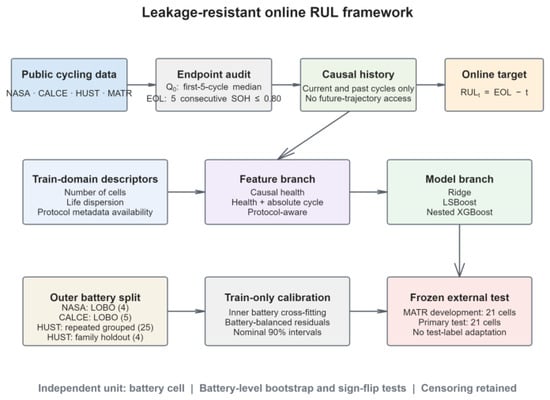
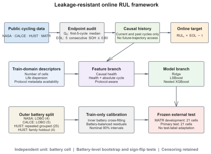
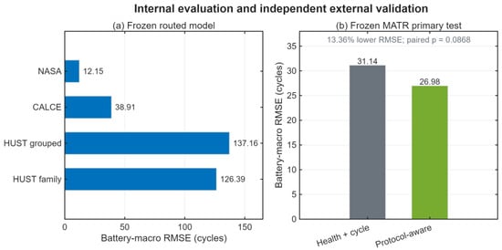
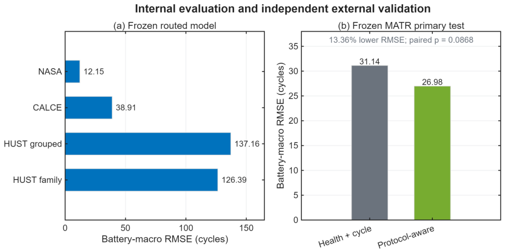
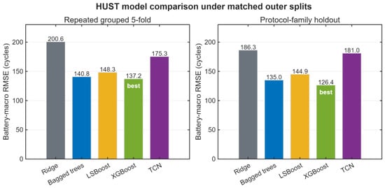
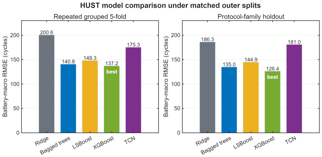
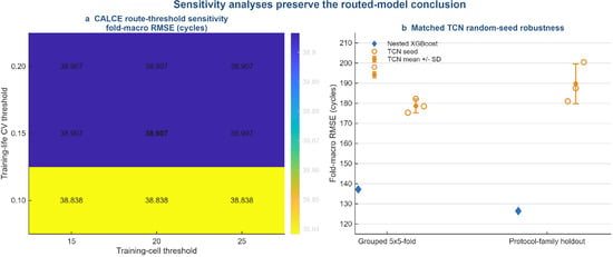
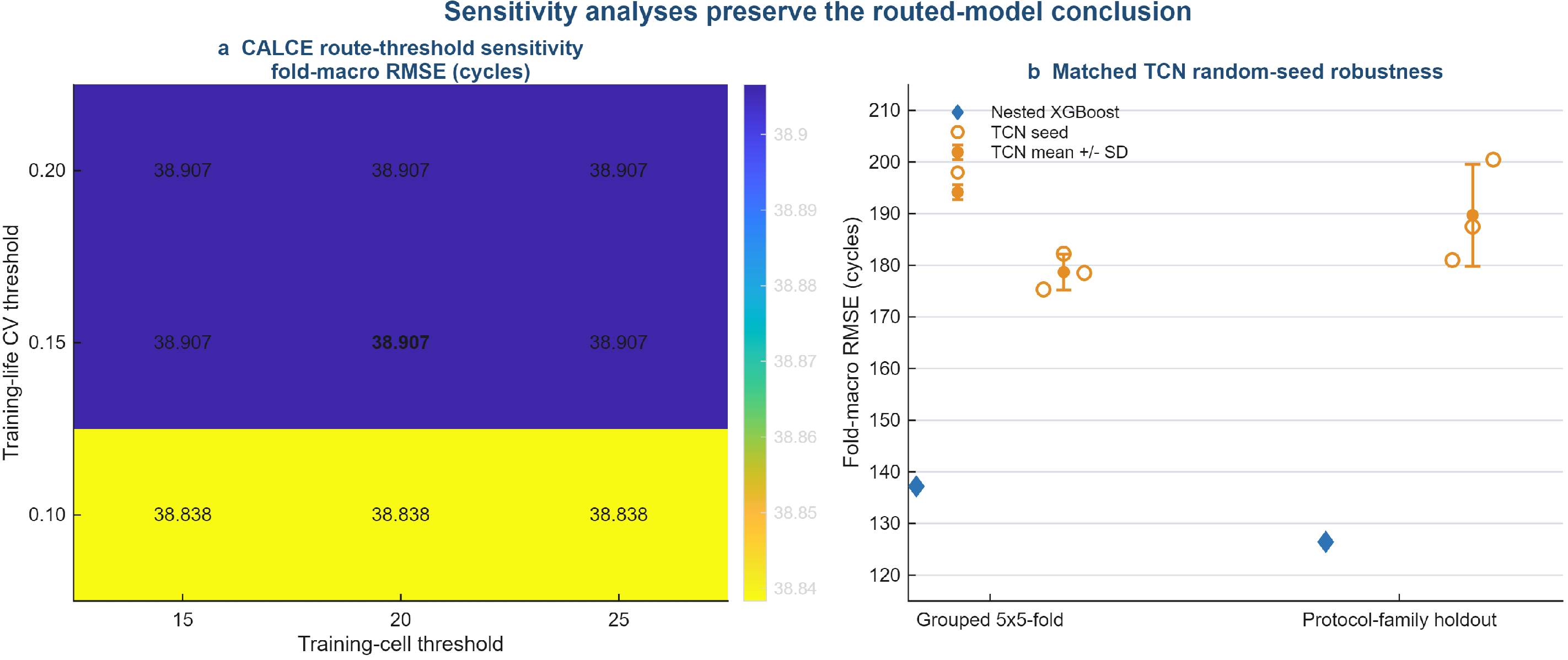
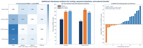
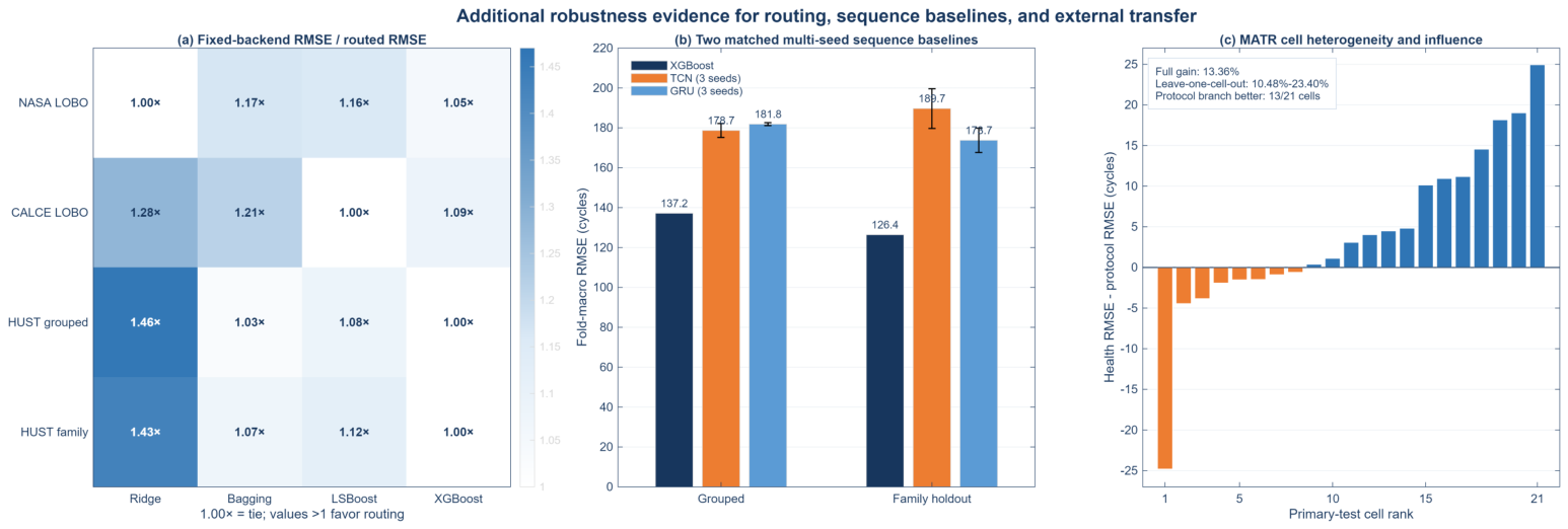
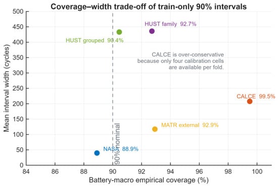
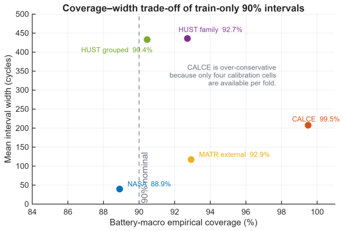
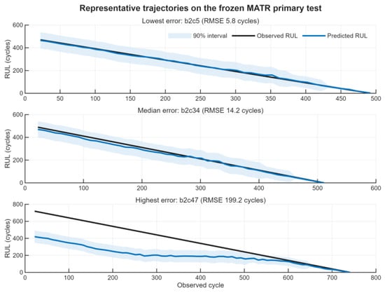
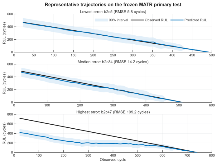
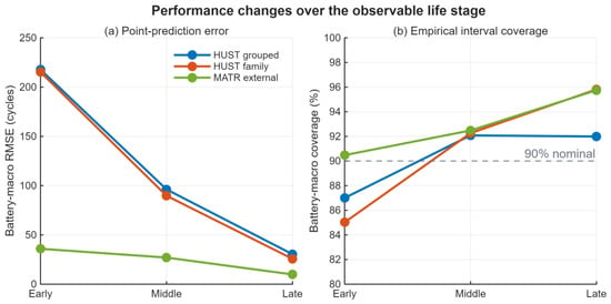
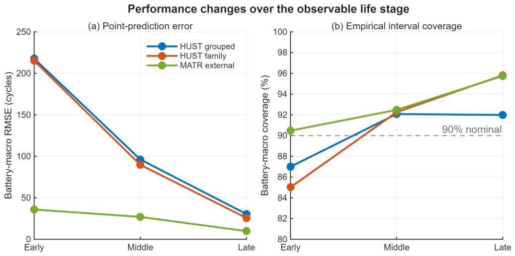

Disclaimer/Publisher’s Note: The statements, opinions and data contained in all publications are solely those of the individual author(s) and contributor(s) and not of MDPI and/or the editor(s). MDPI and/or the editor(s) disclaim responsibility for any injury to people or property resulting from any ideas, methods, instructions or products referred to in the content. |
© 2026 by the authors. Licensee MDPI, Basel, Switzerland. This article is an open access article distributed under the terms and conditions of the Creative Commons Attribution (CC BY) license.